verification and validation of the general mission ... · verification and validation of the...

Verification and Validation of the General Mission Analysis Tool (GMAT)

Steven P. Hughes1, Rizwan H. Qureshi1 , D. Steven Cooley1, Joel J. K. Parker1, Thomas G. Grubb2

NASA Goddard Space Flight Center, Greenbelt, MD, 20771, USA

This paper describes the processes and results of Verification and Validation (V&V) efforts for the General Mission Analysis Tool (GMAT). We describe the test program and environments, the tools used for independent test data, and comparison results. The V&V effort produced approximately 13,000 test scripts that are run as part of the nightly build-test process. In addition, we created approximately 3000 automated GUI tests that are run every two weeks. Presenting all test results are beyond the scope of a single paper. Here we present high-level test results in most areas, and detailed test results for key areas. The final product of the V&V effort presented in this paper was GMAT version R2013a, the first Gold release of the software with completely updated documentation and greatly improved quality. Release R2013a was the staging release for flight qualification performed at Goddard Space Flight Center (GSFC) ultimately resulting in GMAT version R2013b.

I. IntroductionMAT is a space mission design software system for the design and optimization of missions anywhere in the solar system ranging from low Earth orbit to lunar, Libration point, and deep space missions. The system

contains high-fidelity space system models, optimization and targeting, built-in scripting and programming infrastructure, and customizable plots, reports and data products, to enable flexible analysis and solutions for custom and unique applications. GMAT can be driven from a fully-featured, interactive Graphical User Interface (GUI), or from a custom script language. An important goal of the GMAT project is to share NASA funded technology as openly as possible as required by the Space Act. To this end, most components of GMAT have been released under the Apache License 2.0.

The GMAT V&V effort for R2013a involved 10 full time engineers and developers for approximately 18 calendar months of effort. During that time, no new features were incorporated (in fact, some were removed until quality could be improved). The primary objective of this paper is to describe at a high level the test processes and document key test results. As of the completion of the V&V effort, GMAT was rigorously tested on the Windows 7 platform and we were performing nightly regression tests running almost 12,000 test cases for the script engine and approximately 3400 test cases for the GUI interface. While the system is routinely built on Mac and Linux, we consider the software to be in alpha form on those platforms. The V&V program we present here was used for version R2013a released in April 2013. R2013a is the first Gold version of the system. After release R2013a, we performed further flight qualification of the system that is described by Qureshi1, resulting in version R2013b, the first flight qualified release of GMAT.

We begin the paper with a high-level overview of GMAT including a description of the software, its history, and usage. We then provide a high level overview of the V&V program including the driving goals and philosophy, high-level testing methodology, and the test environments and tools. Detailed discussion of testing methodology and results are presented in five sections devoted to logical grouping of system components. Those sections include Dynamics and Modelling, Powered Flight, Solvers, Output and Utilities, and Programming Infrastructure. A separate section is devoted to GUI testing processes and results.

1 Aerospace Engineer, Navigation and Mission Design Branch2 Software Engineer, Ground Software Systems Branch

G

American Institute of Aeronautics and Astronautics1

https://ntrs.nasa.gov/search.jsp?R=20140017798 2018-08-22T10:08:26+00:00Z

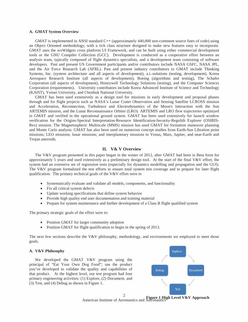
Figure 1 High Level V&V Approach

A. GMAT System Overview

GMAT is implemented in ANSI standard C++ (approximately 440,000 non-comment source lines of code) using an Object Oriented methodology, with a rich class structure designed to make new features easy to incorporate. GMAT uses the wxWidgets cross platform UI Framework, and can be built using either commercial development tools or the GNU Compiler Collection (GCC). Development is conducted as a cooperative effort between an analysis team, typically composed of flight dynamics specialists, and a development team consisting of software developers. Past and present US Government participants and/or contributors include NASA GSFC, NASA JPL, and the Air Force Research Lab (AFRL). Past and present industry contributors to GMAT include Thinking Systems, Inc. (system architecture and all aspects of development), a.i.-solutions (testing, development), Korea Aerospace Research Institute (all aspects of development), Boeing (algorithms and testing), The Schafer Corporation (all aspects of development), Honeywell Technology Solutions (testing), and the Computer Sciences Corporation (requirements). University contributors include Korea Advanced Institute of Science and Technology(KAIST), Yonsei University, and Chonbuk National University.

GMAT has been used extensively as a design tool for missions in early development and proposal phases through and for flight projects such as NASA’s Lunar Crater Observation and Sensing Satellite LCROSS mission and Acceleration, Reconnection, Turbulence and Electrodynamics of the Moon's Interaction with the SunARTEMIS mission, and the Lunar Reconnaissance Orbiter (LRO). ARTEMIS and LRO flew trajectories optimized in GMAT and verified in the operational ground system. GMAT has been used extensively for launch window verification for the Origins-Spectral Interpretation-Resource Identification-Security-Regolith Explorer (OSIRIS-Rex) mission. The Magnetospheric Multiscale (MMS) mission has used GMAT for formation maneuver planning and Monte Carlo analysis. GMAT has also been used on numerous concept studies from Earth-Sun Libration point missions; LEO missions; lunar missions; and interplanetary missions to Venus, Mars, Jupiter, and near-Earth and Trojan asteroids.

II. V& V OverviewThe V&V program presented in this paper began in the winter of 2012, after GMAT had been in Beta form for

approximately 5 years and used extensively as a preliminary design tool. At the start of the final V&V effort, the system had an extensive set of regression tests (especially for dynamics modelling and propagation and the GUI). The V&V program formalized the test efforts to ensure total system test coverage and to prepare for later flight qualification. The primary technical goals of the V&V effort were to

Systematically evaluate and validate all models, components, and functionalityFix all critical system defectsUpdate working specifications that define system behaviorProvide high quality end user documentation and training materialPrepare for system maintenance and further development of a Class B flight qualified system

The primary strategic goals of the effort were to:

Position GMAT for larger community adoption Position GMAT for flight qualification to begin in the spring of 2013.

The next few sections describe the V&V philosophy, methodology, and environments we employed to meet those goals.

A. V&V Philosophy

We developed the GMAT V&V program using the principal of “Eat Your Own Dog Food”; use the product you’ve developed to validate the quality and capabilities of that product. At the highest level, our test program had fourprimary engineering activities: (1) Explore, (2) Document, and (3) Test, and (4) Debug as shown in Figure 1.


Figure 2 High Level Test Process and Environment

During the Explore phase, test engineers explored and used system components and documented their findings as pre-triage/sanity checks to determine the state of the component. The documentation activity included updating working specifications, writing additional test plans/procedures, and updating or writing end-user documentation. The testing phase included writing and performing additional tests to ensure full test coverage. We found that the Explore, Document, and Test activities are not necessarily sequential. As testing occurred, additional information was identified that is useful to users and that should be included in specifications and user documentation. During documentation, additional areas of exploratory and beta testing were identified. It was not unusual to make a few cycles through these activities for a given component.

B. V&V Methodology

We employed industry standard V&V methodologies throughout the test program. The GMAT Software Management Plan9 and Test Plan10 provided guidance for basic test processes. Test engineers developed specific test procedures and test cases according to the plans for all components in scope of the V&V program. A major goal of the V&V program was to implement test procedures and test cases in repeatable and automated test environments to support regression testing of the entire application during current and future development activities. A high level view of the test process and environment are illustrated in Figure 2. The regression test environments are discussed in the next section.

Table 1 describes the primary test classes performed by test engineers. Note: developer testing such as integration and unit tests are performed during the development process and are not discussed here.

We logically grouped system components in the V&V program into subgroups shown in Table 2. Each component area was assigned a Flight Dynamics Engineer (FDE) to lead the V&V effort for the area and a Software

Table 1. Primary System Test Types

Test Type DescriptionNumeric Tests Tests of physical and mathematical models. Numeric tests are performed by

comparing output to external "truth".Functional tests Tests that verify non-numeric functionality, such as plotting styles, file formats,

and control flow behavior.Input validation Tests that ensure user inputs are validated by the system and the correct error

messages are provided for invalid user input.End-to-end tests Tests that solve an end-to-end engineering problem such as a lunar transfer or

orbital maneuver. These tests are "fit for use" tests and are applications of GMAT to real-world problems

Stress Tests Test designed to stress the system and make heavy use of system resources.Edge corner tests Tests designed to test models at the boundaries of applicability, in the GMAT

context this often means testing models near numerical singularities.


Development Engineer (SDE) responsible for addressing defects found during testing. In all, about 65 componentswere tested. The FDE was responsible for the Explore, Document, and Test activities for features in the component group, and the SDE was responsible for defect resolution and review of work products such as specifications and user documentation. The GMAT Configuration Control Board (CCB) met weekly to triage all issues found during testing. We tracked high level progress using standard agile burn down charts tracking number of open critical and minor issues, and number of features remaining to be tested and documented.

C. V&V Environment

The environment required to support the V&V program is a complex set of tools that must meet requirements for test automation and traceability for all interfaces including the GMAT script interface and the GMAT GUI interface. We developed a custom script test environment in MATLAB2 to perform automated script regression testing and used SmartBear Software’s TestComplete3 for automated GUI testing. The automation requirements on the test environment help reduce human error in testing processes and ensure that the large number of test cases and procedures can be executed in a repeatable and efficient manner. To meet these goals, the test environment must be able to run a large number of test types and compare very different types of output to benchmark data.

GMAT's script test system is written in MATLAB and automatically runs all test cases, compares the results to both external benchmark data and past GMAT output, and sends nightly test reports to the entire development team. Nightly regression test reports contain high-level statistics on the number of tests run and the number of failing tests. The reports also document test case changes including tests that have switched from passing to failing, test that changed from failing to passing or tests that changed but still fail or pass. Custom script verification tests types ensure that all features implemented in GMAT function correctly and within tolerance and allow for rapiddevelopment of new test cases without needing to understand the internals of the test system. The system currently supports about 15 built-in “Comparators” such as the ability to compare position velocity files to external benchmark data, compare generic data files to user defined tolerances, perform file difference compares, and search system log files for warnings or error messages. Testers can quickly run test cases by specific software requirement ID, test name, or feature group among others. Additionally, script tests are classified by their type (Numeric, Validation, System, Stress, etc.) and subsets can be run easily by specifying the test categories in the test system configuration. Finally, there are several higher-level classifications of script tests used during the development

Table 2. V&V Logical Component Groupings

Component Area Description/FeaturesDynamics/Models Numerical models for orbit and attitude propagation, solar system and coordinate

system models including spacecraft orbit state representations, spacecraft ballistic and mass properties, spacecraft epoch representations, spacecraft attitude representations, spacecraft kinematic attitude modelling, solar system ephemerides, celestial body modelling, SPICE propagator, numerical integrators, orbital dynamics models, formations, coordinate systems, barycenters, libration points, and the propagation command.

Powered Flight Numerical models for impulsive and finite maneuvering including tanks, thrusters, impulsive maneuver, finite maneuver, and the commands to control maneuvers during the simulation.

Solver Infrastructure Algorithms and infrastructure for solving boundary value and optimization problems. Includes differential corrector and Nonlinear Programming (NLP) solvers, and the commands used to define control variables, cost, and constraint functions in the simulation.

Programming Infrastructure

Algorithms and features for customization including custom scripting, user definedvariables and arrays, scripted custom equations, built-in astrodynamic computations, control flow, and external interfaces.

Output\Utils Components to support graphical and data output such as xy-plots, 3-D graphics, report files, and ephemeris files, as well as the command infrastructure to control output behavior during the simulation.

Application Control Inherently interface elements such as file menus, command line interfaces, and the script editor.


process before committing new code or used nightly to determine if code additions or changes have caused unexpected adverse effects. These higher level categories such as “Smoke” and “System Tests” are groupings of lower level test cases and provide developers and testers insight into the system without running the entire test suite.

The GMAT GUI test environment uses SmartBear Software’s TestComplete to perform automated GUI testing on the Windows platforms. At its most basic level, GUI testing requires clicking on every button and widget in the GMAT GUI, entering valid, invalid, and boundary conditions input into every text widget, and assessing that the GUI responds to all inputs and displays all results correctly. Manually performing these actions is error-prone, labor-intensive, and impossible to repeat every time a change is made to the system. At a more advanced level, GUI testing requires inputting all user data to solve complex engineering problems and verifying the results against benchmark data. Similarly to the script test environment, the GUI test environment is executed from a high level driver that automatically executes GUI tests by test classification and reports on test status and coverage. GUI tests are subcategorized into Unit, Smoke and System tests to allow testers to run subsets of the GUI test cases as the entire test suite currently takes approximately 5 days to run and analyze.

We generated external benchmark data from legacy systems and simple standalone MATLAB implementations depending upon several factors including availability, ease of use, supported features, and trustworthiness of the models and results. Benchmark data and test approaches are discussed in detail with the component discussions in the next section as benchmark tools were selected on a component basis. However, some tools were used more often than others, and we present high-level benchmark tools here. For orbit propagation and other dynamics and modeling evaluation, STK4, FreeFlyer5 and MATLAB propagators were employed to create independent benchmarkdata. For 3-D graphics comparisons, we used Celestia6 and STK. For 2-D plots, we used MATLAB as the external benchmark. Finally, for testing of the script language, and especially mathematical equation parsing, we also used MATLAB as the benchmark tool.

III. Dynamics and Modelling Test Methodology and ResultsThe core of an astrodynamics simulation and design environment are its physical models. For the V&V

program, the Dynamics and Modelling feature group was composed of the following GMAT features: spacecraft orbit state representations, spacecraft ballistic and mass properties, spacecraft epoch representations, spacecraft attitude representations, spacecraft kinematic attitude modelling, solar system ephemerides, celestial body modelling, SPICE propagator, numerical integrators, orbital dynamics models, formations, coordinate systems,barycenters, Libration points, and the propagation command. (Note: GMAT supports impulsive and finite maneuvers models and those are categorized in the Powered Flight component group.) For this paper, we chose to present tests results for Force Modelling, Coordinate Systems, and Numerical Integrators. However, we performed extensive, systematic testing on all components in this group using similar methods for the limited subset we have space to address in this work. The last subsection in this section describes at a high level the test methodology used for other Dynamics and Modelling components not addressed in detail in this paper.

A. Dynamics Models

The orbital dynamics model test approach compared numerical propagation results from GMAT to propagation performed in independent tools such as STK, MATLAB, and FreeFlyer. Orbit test cases included the following regimes: LEO, MEO, HEO, GEO, Lunar, interplanetary, planetary, planetary moon, asteroid, Earth Moon Librationpoint, and Sun-Earth Moon Libration point. We tested dynamics models individually for selected orbit test cases, and tested the superposition of all applicable models for selected orbit test cases. The force models tested includedharmonic gravity, point-mass perturbations, drag (spherical with MSISE-90, MSISE-86, and MSISE-NRL), solar radiation pressure, solid Earth tides, and relativity. When selecting from all permutations of orbit types and dynamics models, and for different solar system configurations, we created approximately 270 unique propagation tests of which approximately 70 are presented below.

Initial state vectors for selected orbital regimes are presented in Table 3 Many Earth orbit state vectors and epochs are consistent with those used by Vallado7. All state vectors are expressed with respect to the natural central body for the orbit test case (i.e. the Moon test case has Moon at the origin) and with respect to the Earth’s mean equator of J2000 axis system. The dynamics model tests employed a single integrator that is available in both GMAT and STK (RKV89). We selected integrator settings to allow precise comparison between tools. These tests employed, for the most part, fixed flux settings for SRP and Drag, and a fixed error control setting. Table 4 contains the initial epochs, time of flight, and output frequency for selected test cases.


Representative test comparison data is shown below for selected orbit propagation test cases in Table 5. Test data is the maximum RSS position error in meters over the test case propagation duration. Velocity comparisons were also included in the test analysis, and were consistently two to four orders of magnitude lower than the position error. Inalmost all test cases, RSS comparisons demonstrated sub meter level agreement between tools. In most cases, cm to mm level agreement is seen.

Table 4 Dynamics Model Test Epochs and DurationsTest Case TOF (days) Initial Epoch Output Step

LEO (SunSync) 1 01 Jun 2004 12:00:00.000 60 sec LEO (ISS) 1 01 Jun 2004 12:00:00.000 60 sec GEO 7 01 Jun 2004 12:00:00.000 600 sec MEO 2 01 Jun 2004 12:00:00.000 120 sec HEO 3 01 Jun 2004 12:00:00.000 300 sec Venus 3 01 Jun 2004 12:00:00.000 300 sec Luna 3 01 Jun 2004 12:00:00.000 300 sec Mars 3 01 Jun 2004 12:00:00.000 300 sec Asteroid/Comet 0.3125 13 Dec 2019 18:01:15.433 N/A Titan 1 01 Jun 2004 12:00:00.000 100 sec Sun-Earth L2 180 05 Feb 2006 17:05:48.772 1/2 day Earth-Moon L2 14.028 23 Jan 2010 00:00:04.000 2400 sec Deep Space 365 01 Jan 2000 12:00:00.000 1 day Lunar Flyby 5.78 23 Jul 2014 20:49:23.867 2000 sec Mars Transfer 312 18 Nov 2013 19:57:09.235 1 day

Table 3 Dynamics Model Test Initial State VectorsX (km) Y (km) Z (km) VX (km/s) VY (km/s) VZ (km/s)

LEO (Sun-Sync) -2290.30106 -6379.47194 0 -0.883923 0.317338 7.610832LEO (ISS) -4453.78359 -5038.20376 -426.384456 3.831888 -2.887221 -6.018232GEO 36607.35826 -20921.7237 0 1.525636 2.669451 0MEO 5525.33668 -15871.1849 -20998.9924 2.750341 2.434198 -1.068884HEO -1529.89429 -2672.87736 -6150.11534 8.717518 -4.989709 0Venus -4832.07438 0 4832.074381 -0.64535679 -7.3662402 0.645356787Luna -1486.79212 0 1486.792117 -0.14292773 -1.63140762 0.142927729Mars -2737.48165 0 2737.481646 -0.31132169 -3.55349231 0.311321695Asteroid/Comet -0.32956666 0.189673215 -0.30304989 1.78534E-05 -8.8048E-05 -7.4522E-05Titan 250.4443812 -2420.44525 -1049.39145 1.832446416 0.159603524 0.069196596Sun-Earth L2 1010800.968 -910963.538 -295145.631 0.264285265 0.286744175 0.07338745Earth-Moon L2 406326.2266 177458.3876 145838.5808 -0.51727467 0.774650367 0.331416603Deep Space 56937994.01 -1713823.5 1657873.06 0.045105343 10.61438285 4.735060583Lunar Flyby 7482.854524 -4114.93842 -1171.25835 4.436048586 8.268589685 -1.56960804Mars Transfer 3757.045995 4552.470526 -2656.97254 -9.5153199 6.14681789 -2.66380712


For selected orbital test cases, we performed superposition tests where all or nearly all supported dynamics models were included simultaneously. Approximately 80 superposition tests were performed, with representative results shown in Table 6. Propagator sectioning tests -- where the propagation origin is changed at the sphere of influence –were performed for the Lunar Transfer and Mars Transfer test cases. In general, all tests agreed at the meter level, and many tests agree at the centimeter level.

Table 6 Combined Dyanamics Model Test Results

Test Case IDMax PositionDiff. RSS (m)

GEO (TBPM,HG,Drag,SRP,Tide) 9.2227E-01GEO (TBPM,HG,Drag,SRP) 1.7184E-04GPS (TBPM,HG,Drag,SRP,Tide) 5.2289E-01GPS (TBPM,HG,Drag,SRP) 7.5020E-02ISS (TBPM,HG,Drag,SRP,Tide) 1.9932E+00ISS (TBPM,HG,Drag,SRP) 1.6639E+00Molniya (TBPM,HG,Drag,SRP,Tide) 6.3083E+00Molniya (TBPM,HG,Drag,SRP) 5.1301E-01SunSync (TBPM,HG,Drag,SRP,Tide) 1.4991E+00SunSync (TBPM,HG,Drag,SRP) 3.3214E-01Lunar Transfer (TBPM, HG, SRP) 8.6480E-01Mars Transfer (TBPM, HG, SRP) 5.2626E+00Asteroid (TBPM, HG, SRP) 4.6731E-03Earth Moon L2 (TBPM, SRP) 8.0749E-01Deep Space (TBPM, Rel) 3.8275E-02Titan(TBPM, SRP) 2.5002E-01

Table 5 Individual Dynamics Model Test ResultsDynamics Model

Orbital Regime

Sphe

rical

Gra

vity

Har

mon

ic g

ravi

ty

Tide

s

Poin

t mas

s per

turb

atio

n

SRP

MSI

SE90

NR

LMSI

SE00

Jacc

hia-

Rob

erts

Rel

ativ

istic

Cor

rect

ion

ISS 7.1E-06 2.5E-03 3.3E-01 1.5E-05 1.3E-01 1.8E-01 1.1E+00 1.9E+00 3.8E-02Sun Sync 3.9E-05 5.0E-04 5.7E-01 3.6E-05 1.7E-01 1.8E-02 5.8E+00 2.0E+00 xGPS 2.7E-06 1.5E-04 2.5E-02 2.3E-05 4.7E-02 1.4E-05 4.2E-06 2.7E-06 xGEO 6.3E-06 2.8E-05 5.0E-02 1.8E-04 2.4E-05 6.3E-06 5.2E-05 6.3E-06 2.3E-03Molniya 2.4E-04 6.1E-03 6.0E+00 2.0E-04 5.8E-01 1.8E-03 4.3E+00 1.3E-01 xLuna 7.3E-05 1.9E-04 N/A 2.2E-04 1.1E-04 N/A N/A N/A xVenus 9.0E-03 1.1E-02 N/A 1.4E-02 3.7E-02 N/A N/A N/A xMars 6.1E-02 1.2E-01 N/A 3.2E-01 6.0E-01 N/A N/A N/A x


Vallado7 compared orbit propagation results from several software systems including TRACE, GEODYN, GTDS, Special K, and STK HPOP. A detailed case-by-case comparison is beyond the scope of this work. However, we analyzed results from Vallado and extracted the maximum RSS propagation difference for selected orbits tested and compared those differences to those between STK and GMAT. High-level order of magnitude comparisons are shown in Table 7. Note that most test cases presented by Vallado had significantly better agreement than those presented in the table, and the data presented only compares worst case agreement among tools to aid in identifying an upper bound on expected agreement. The differences between STK and GMAT are in line with the differencesseen between STK and other programs with the notable exception that point mass perturbations and drag propagations are orders of magnitude smaller between GMAT and STK than between STK and other programs tested when comparing worse case scenarios.

B. Numerical Integrators

We tested GMAT’s numerical integrators using “closure” tests that apply each integrator to a set of cases that demonstrate the integrator’s accuracy and performance characteristics in different orbital regimes. Closure is tested by integrating an initial state forward for an appropriate duration, then integrating backwards to the initial epoch and comparing the integrated solution to the initial state vector. An ideal integrator would yield the identical initial state after propagation to within round-off error dictated by precision of the computer. We tested 6 orbit types described in Table 8. For all test cases, the error control setting was set to relative error with respect to the step size where the relative error tolerance was set to 1e-12 for all integrators except for Adams-Bashfourth-Moulton (45), which was set to 1e-11 because of poor performance. For more information on the integrators implemented in GMAT, see the GMAT User Guide8

.

Table 9 contains integrator accuracy and performance data for numerical integrator tests. The error values in the table are the RSS difference of the final position after forward and backward propagation to the initial epoch. The run time data for each orbit type is normalized on the integrator with the fastest run time for that orbit type.

Table 8 Integator Test Case DescriptionsOrbit Dynamics Model Duration

LEO Earth 20x20, Sun, Moon, MSISE90 density, SRP 1 day

Molniya Earth 20x20, Sun, Moon, Jacchia Roberts, SRP 3 days

Mars Transfer

Near Earth: Earth 8x8, Sun, Moon, SRP

333 days Deep Space: All planets as point mass perturbationsNear Mars: Mars 8x8 SRP

Lunar Transfer Earth central body with all planets as point mass perturbations 5.8 days

Finite Burn (case 1 and 2) Point mass gravity. (1) Blow down, (2) Pressure Regulated. 7200 sec.

Table 7 Worst Case, Max RSS Position Differences (m) for Selected Orbit Test CasesBetween DifferentOrbit Propagation Software and STK.

SoftwareHarmonic Gravity

Point Masses SRP Drag

GTDS 0.07 0.06 2.50 575.00TRACE 0.0020 0.02 1.50 750.00Special K N/A 0.07 N/A N/AGMAT 0.01 0.0002 0.58 5.77GEODYN N/A N/A N/A 1000


In most cases, mm to cm accuracy is achieved, especially for higher order integrators such as the Runge Kutta Verner (89) and the Prince Dormand (78). Comparing the run time data for each integrator shown in the table below we see that the PrinceDormand78 integrator was the fastest for 4 of the 6 cases and tied with the RungeKutta89integrator for LEO test case. For the Lunar flyby case, the RungeKutta89 was the fastest integrator; however, in this case the PrinceDormand78 integrator was at least 2 orders of magnitude more accurate given equivalent accuracysettings. Notice that the AdamsBashforthMoulton integrator has km level errors for some orbits because it is a low-order integrator (45). The RKN68 is a second order integrator and cannot be used for finite burn modelling so results are not presented for those cases.

C. Coordinate Systems

GMAT supports numerous coordinate system types ranging from standard inertial systems such as Fifth Fundamental Catalogue (FK5) and the International Celestial Reference Frame (ICRF), as well as time varying systems such as Local Vertical Local Horizontal (LVLH), Velocity Normal Bi-Normal (VNB), Body Fixed, and Earth Mean of Date Equator to name a few. In R2013a, 19 axis types are supported. For a more detailed discussion of the coordinate systems in GMAT see the GMAT User Guide8.

All coordinate systems were extensively tested by performing transformations to and from all supported coordinate system types resulting in approximately 450 unique coordinate conversion test cases. Some time dependent coordinate systems, such as the International Terrestrial Reference Frame (ITRF), were tested by propagating representative orbits using a two-body dynamics model, and comparing the propagated state vectors at each propagation time to benchmark data. The primary source of benchmark data was STK; however, MATLAB was used for Object Referenced (LVLH, VNB, etc.) axes, the Geocentric Solar Magnetic (GSM) axes, and for body fixed axes of the celestial bodies other than Earth and Moon.

Comparison test data for selected test cases is shown in Table 10 for conversion of a circular LEO state vector with semi major axis of 6800 km. We include RSS differences and angular differences for both position and velocity transformations. Angular position differences are all on the order of 5e-8 degrees and in many cases much smaller, with position differences at the mm level or better. Velocity RSS comparisons show micro-meter per second agreement and angular comparisons are on the order of 5e-8 degrees or smaller.

Table 9 Integrator Test DataOrbit Data RKV89 RKN68 RK56 PD45 PD78 ABM

ISS Run Time 1.53 1.00 2.14 2.78 1.46 3.41 Error (m) 0.003 64.060 0.022 0.002 0.006 0.012

Molniya Run Time 1.32 1.47 1.99 3.08 1.00 3.35 Error (m) 0.007 0.601 0.059 0.032 0.043 380.125

Lunar Flyby Run Time 1.00 1.01 2.26 2.98 2.21 3.30 Error (m) 0.063 0.017 0.002 0.023 0.000 0.236

Mars Transfer

Run Time 1.02 1.04 1.14 1.40 1.00 3.07 Error (m) 0.030 0.001 0.043 0.194 0.009 25.231

Finite burn 1 Run Time 1.27 N/A 1.24 1.26 1.00 1.45 Error (m) 0.002 N/A 0.006 0.002 0.002 0.000

Finite burn 2 Run Time 1.03 N/A 1.18 1.31 1.00 1.54 Error (m) 0.002 N/A 0.000 0.000 0.001 0.003


D. Other Dynamics and Modelling Components

The Dynamics and Modelling component group contained 13 components, and in this paper we only presented test results for three of those components. The remaining 10 components all received equally rigorous testing during the V&V program. Table 11 contains brief descriptions--focusing on numeric system tests descriptions--of the baseline data source and methodology used for other components in the dynamics group.

Table 10 Coordinate System Test ResultsConversion Type Position Comparison Velocity Comparison

RSS

Diff (m) Angle Diff

(deg.) RSS

Diff (m/s) Angle Diff

(deg.) FK5 To BodyFixed 5.79E-03 4.88E-08 5.65E-06 4.23E-08 FK5 To BodySpinSun 2.17E-04 1.83E-09 1.35E-07 1.01E-09 FK5 To GSE 1.11E-05 9.36E-11 1.22E-08 9.14E-11 FK5 To GSM 2.13E-04 1.79E-09 3.66E-06 2.74E-08 FK5 To ICRF 7.80E-03 6.57E-08 1.97E-06 1.47E-08 FK5 To MJ2000Ec 9.19E-05 7.74E-10 1.05E-07 7.84E-10 FK5 To MJ2000Eq 0.00E+00 0.00E+00 6.39E-12 4.78E-14 FK5 To MODEc 3.33E-07 2.80E-12 2.31E-11 1.73E-13 FK5 To MODEq 9.37E-10 7.90E-15 6.53E-12 4.89E-14 FK5 To MOEEc 6.75E-09 5.69E-14 5.42E-12 4.06E-14 FK5 To MOEEq 4.90E-09 4.13E-14 6.14E-12 4.59E-14 FK5 To ObjectReferenced 1.11E-05 9.36E-11 1.22E-08 9.14E-11 FK5 To TODEc 2.00E-04 1.69E-09 2.20E-07 1.65E-09 FK5 To TODEq 1.98E-04 1.67E-09 2.38E-07 1.78E-09 FK5 To TOEEc 6.55E-05 5.52E-10 7.20E-08 5.39E-10 FK5 To TOEEq 2.05E-04 1.72E-09 2.57E-07 1.92E-09 FK5 To Topocentric 5.92E-03 4.99E-08 5.68E-06 4.25E-08


IV. Powered Flight Methodology and Results

The GMAT Powered Flight feature area consists of resources (i.e., objects) and commands needed to model both impulsive and finite maneuvers. Components in the Powered Flight Group include fuel tanks and thrusters, maneuver models, and commands to control when maneuvers occur in the simulation. The Powered Flight testspresented here focus on the numerical results obtained as a result of a maneuver, such as spacecraft position, velocity, and mass, and are categorized by maneuver type. Section A describes the impulsive maneuver test methodology and results, and Section B describes the finite burn maneuver test methodology and results.

Table 11 Baseline Data Sources and Test Methodology for Other Model ComponentsComponent Test MethodologySolar System Ephemerides

Tested against MATLAB DE file implementation and the MICE toolkit. We compared state vectors to baseline data at different epochs and with respect to multiple coordinate system origins. Results demonstrated excellent agreement.

Libration Point Tested using MATLAB implementations and off-the shelf MATLAB DE ephemeris readers and the MICE toolkit. We compared Libration point locations (all 5) to baseline data at different epochs and with respect to multiple coordinate system origins. Results demonstrated excellent agreement.

Barycenter Tested using MATLAB implementations and off-the shelf MATLAB DE ephemeris readers and the MICE toolkit. We compared solar system and user defined barycenter locations to baseline data at different epochs and with respect to multiple coordinate system origins. Results demonstrated excellent agreement.

Spacecraft Kinematic Attitude Propagation

Tested against MATLAB implementations. Attitude configurations were propagated and compared to benchmark data. Additionally, mode change tests were performed. Results demonstrated excellent agreement.

Spacecraft Attitude Representations

Tested against STK and MATLAB implementations. Attitude initial state conversions were tested to and from all supported representations and compared to benchmark data. Results demonstrated excellent agreement.

Spacecraft Orbit State Representations

Tested against FreeFlyer, STK, and MATLAB implementations. Orbit state representations were converted to and from all supported representations, for each orbit type (Circular, Elliptic, and Hyperbolic) supported by the representation. Results demonstrated excellent agreement.

Celestial Body Model Tested against STK and MATLAB implementations. Shape and orientations models were tested against baseline data for all built-in bodies and all supported types of user-defined celestial body. Results demonstrated excellent agreement.

Propagate Command Tested against STK and MATLAB implementations. Numeric propagation tests were documented in a previous section. Extensive stopping condition testing was performed comparing GMAT to benchmark data. Additionally, multiple spacecraft propagation was extensively tested. Results demonstrated excellent agreement.

Spacecraft Ballistic and Mass Properties

Tested against STK and MATLAB implementations. Various configurations of high and low ballistic coefficient were tested in various orbit regimes such as LEO and HEO and compared to benchmark data. Results demonstrated excellent agreement.

Spacecraft Epoch Tested against STK and MATLAB implementations. Conversion of various test epochs in all supported systems to all other supported systems was performed. Test epochs included leap seconds and leap years. One significant issue was found and is tracked as ticket GMT-2561 in the project issue tracker.


A. Impulsive Maneuvers

We performed over 700 numerical tests to verify GMAT’s implementation of impulsive maneuvers. The tests are categorized by orbit type, spacecraft configuration, impulsive burn configuration, choice of maneuver coordinate system (CS), and fuel tank configuration. We modeled three different orbit types, corresponding to a spacecraft in an Earth orbit, a lunar orbit, and a Mars orbit. The initial conditions, at a TAI modified Julian epoch of 21545, are specified in Table 12 in Earth mean equator J2000 (MJ2000Eq) coordinates relative to the body specified in the orbit type.

For all the orbit types above, we used a simple point mass force model, with no other perturbing forces, designed to make it easier to analyze the effects of maneuvers. The Earth orbit case models only Earth gravity with equal to 398600.4415 km3 s-2. Analogously, the Moon and Mars cases use values of 4902.7991 km3 s-2 and 42828.2866 km3 s-2, respectively.

We modeled seven different impulsive burn configurations which use different values for the V vector, gravitational acceleration and ISP values used to calculate fuel use, and choice of whether or not to model fuel depletion. We also modeled five different choices of maneuver coordinate systems (CS). These include both inertial and non-inertial coordinate systems as defined in Table 13.

GMAT models two types of fuel tank, a blow down (BD) tank and a pressure regulated (PR) tank. As shown in Table 14, there were 22 different fuel tank configurations modeled, 11 blow down tank configurations and 11 pressure regulated tank configurations. Except for the pressure model used, the 11 blow down tank configurations are identical to the pressure regulated configurations. The 11 different configurations used different values of fuel tank characteristics such as initial fuel mass, fuel density, temperature, reference temperature, initial pressure, and

Table 13 Coordinate Systems Used in Impulsive Maneuver TestingCoordinate System Designation Description

MJ2000Eq CS0 J2000-based Earth-centered Earth mean equator inertial Earth VNB

CS1

Earth Velocity-Normal-Binormal (VNB) is a non-inertial coordinate system based upon the motion of the spacecraft with respect to the Earth. The X-axis of this coordinate system is along the velocity of the spacecraft with respect to the Earth, the Y-axis is along the instantaneous orbit normal (with respect to the Earth) of the spacecraft, and the Z-axis completes the right-handed set.

Earth LVLH CS2 Earth Local Vertical Local Horizontal (LVLH) is a non-inertial coordinate system based upon the motion of the spacecraft with respect to the Earth. The X-axis of this coordinate system is the position of the spacecraft with respect to the Earth, the Z-axis is the instantaneous orbit normal (with respect to the Earth) of the spacecraft, and the Y-axis completes the right-handed set.

SpacecraftBody CS3 SpacecraftBody is the attitude system of the spacecraft. Since the thrust is applied in this system, GMAT uses the attitude of the spacecraft, a spacecraft attribute, to determine the inertial thrust direction.

Custom Designed Earth VNB

CS4 Same coordinate system as Earth VNB. (created using a different user interface)

Table 12 Impulsive Maneuvers Test Initial State VectorsOrbit Type X (km) Y (km) Z (km) VX (km/s) VY (km/s) VZ (km/s)

Earth 7653.768 0 0 0 7.2166 0Moon 2085.84 0 0 0 1.5331 0

Mars 4076.4 0 0 0 3.2414 0


volume. For the test results we will show, we used Tank A as the baseline tank. Values that differ from the baseline tank are highlighted in red.

The various test cases have names such as IBurn_Earth_ScA_IBA_CS0_TankA, which we now explain. “IBurn” is used to indicate that this is an Impulsive Burn test. “Earth” indicates that we are using the Earth orbit type. “ScA” is used to indicate that we are using the Spacecraft A configuration. “IBA” indicates that we are using the Impulsive Burn A configuration. “CS0” indicates that we are using the maneuver coordinate system CS0 configuration. Finally, “TankA” indicates that we are using the Fuel Tank A configuration. The impulsive burn tests applied an impulsive V and then checked the final position, velocity, and mass against MATLAB-generated truth results and FreeFlyer. The test case IBurn_Earth_ScA_IBA_CS0_TankA is the baseline test for the impulsive burn tests. In all the test results that follow, each test used the same configuration as the baseline test except for the one parameter that is varied in each table. The table of results below varies the orbit type.

Table 15 Orbit Type Results for Impulsive ManeuversOrbit Position RSS Error

(m)Velocity RSS Error

(m/s)Mass Error

(g)Earth 0 0 2.27374E-10Moon 2.59206E-08 0 2.27374E-10Mars 5.96083E-06 1.7764E-12 2.27374E-10

The position RSS error ranged from 0 to approximately 6.0e-6 m, the velocity RSS error ranged from 0 to approximately 1.8e-12 m/s. All of the cases had a mass error of approximately 2.3e-10 g. We note that the Earth case had the smallest overall error. This is probably because both the spacecraft state and the V vector are specified in the same coordinate system (MJ2000Eq) and thus no coordinate transformations had to be performed.

Table 14 Fuel Tank ConfigurationsTank Description Mass

(kg)Pressure

(kPa)Temp

(C)Ref

Temp(C)

Volume(m3)

FuelDensity(kg/m3)

PressureModel

A Baseline 725 1200 20 12 0.8 1029 PRB High Mass 820 1200 20 12 0.8 1029 PRC High Pressure 725 2500 20 12 0.8 1029 PRD Low Pressure 725 725 20 12 0.8 1029 PRE High Temp 725 1200 200 12 0.8 1029 PRF Low Temp 725 1200 2 12 0.8 1029 PRG High Ref

Temp 725 1200 20 100 0.8 1029 PR

H Low Ref Temp 725 1200 20 2 0.8 1029 PR

I High Volume 725 1200 20 12 80 1029 PRJ Low Density 725 1200 20 12 8.0 101.325 PRK High Density 725 1200 20 12 0.8 2500 PRL Baseline (BD) 725 1200 20 12 0.8 1029 BDM High Mass 820 1200 20 12 0.8 1029 BDN High Pressure 725 2500 20 12 0.8 1029 BDO Low Pressure 725 725 20 12 0.8 1029 BDP High Temp 725 1200 200 12 0.8 1029 BDQ Low Temp 725 1200 2 12 0.8 1029 BDR High Ref

Temp 725 1200 20 100 0.8 1029 BD

S Low Ref Temp 725 1200 20 2 0.8 1029 BD

T High Volume 725 1200 20 12 80 1029 BDU Low Density 725 1200 20 12 8.0 101.325 BDV High Density 725 1200 20 12 0.8 2500 BD


Table 16 varies the maneuver coordinate system. All of the cases had zero position and velocity RSS error and a mass error of approximately 2.3e-10kg.

Table 16 Maneuver Coordinate System Results for Impulsive ManeuversCoordinate System Position RSS Error


(m/s)Mass Error

(g)Earth Mean Equator J2000 (CS0) 0 0 2.27374E-10

Earth VNB (CS1) 0 0 2.27374E-10Earth LVLH (CS2) 0 0 2.27374E-10

SpacecraftBody (CS3) 0 0 2.27374E-10Custom Designed Earth VNB (CS4) 0 0 2.27374E-10

Table 17 varies the tank configuration. All of the cases had zero position and velocity RSS error. All of the cases had 0 mass error except for the high mass tanks, Tanks B and M, which had a mass error of approximately 2.3e-10 grams.

Table 17 Tank Configuration Results for Impulsive ManeuversTank

ConfigurationPosition RSS

Error (m)

Velocity RSS Error(m/s)

Mass Error(g)

A 0 0 2.27374E-10B 0 0 0C 0 0 2.27374E-10D 0 0 2.27374E-10E 0 0 2.27374E-10F 0 0 2.27374E-10G 0 0 2.27374E-10H 0 0 2.27374E-10I 0 0 2.27374E-10J 0 0 2.27374E-10K 0 0 2.27374E-10L 0 0 2.27374E-10M 0 0 0N 0 0 2.27374E-10O 0 0 2.27374E-10P 0 0 2.27374E-10Q 0 0 2.27374E-10R 0 0 2.27374E-10S 0 0 2.27374E-10T 0 0 2.27374E-10U 0 0 2.27374E-10V 0 0 2.27374E-10

As shown in Table 18 below, summarizing all impulsive maneuver results, the position RSS error ranged from 0 to approximately 6.0e-6 m, the velocity RSS error ranged from 0 to approximately 1.8e-12 m, and the mass error ranged from 0 to approximately 2.3e-10 g.


Table 18 Summary of Impulsive Maneuver ResultsTest Category Position RSS Error (m) Velocity RSS Error (m/s) Mass Error (g)

Low High Low High Low HighOrbit 0 6.0e-6 0 1.8e-12 2.3e-10 2.3e-10

Maneuver Coordinate System 0 0 0 0 2.3e-10 2.3e-10Tank Configuration 0 0 0 0 0 2.3e-

10All 0 6.0e-6 0 1.8e-12 0 2.3e-

10

B. Finite Maneuvers

We performed over 900 numerical tests to verify GMAT’s implementation of finite burn maneuvers. The tests are categorized by orbit type, spacecraft configuration, thruster configuration, choice of maneuver coordinate system (CS), and fuel tank configuration.

We modeled ten different orbit types, corresponding to a spacecraft in an orbit about each of the planets, Pluto,and the moon. As was the case for impulsive maneuvers, for all the orbit types above, we used a simple point mass force model with no other perturbing forces, designed to make it easier to analyze the effects of maneuvers. The initial conditions, at a TAI modified Julian epoch of 21545, are specified below in Earth mean equator J2000 coordinates (MJ2000Eq) relative to the body specified in the orbit type. In addition, the Table 19 below includes the

value used for each orbit type.

Table 19 Finite Maneuvers Test Initial State VectorsOrbit Type (km3/s2) X (km) Y (km) Z (km) VX (km/s) VY (km/s) VZ (km/s)Mercury 22032.0805 2927.64 0 0 0 2.7433 0Venus 324858.7656 7262.28 0 0 0 6.6882 0Earth 398600.4415 7653.768 0 0 0 7.2166 0Moon 4902.7991 2085.84 0 0 0 1.5331 0Mars 42828.2866 4076.4 0 0 0 3.2414 0Jupiter 126712597.0818 85790.4 0 0 0 38.4318 0Saturn 37939519.7088 72321.6 0 0 0 22.904 0Uranus 5780158.5336 30670.8 0 0 0 13.728 0Neptune 6871307.7715 30322.8 0 0 0 15.0534 0Pluto 1020.8649 1381.2 0 0 0 0.85972 0

The finite burn maneuver tests used a single spacecraft configuration with specific values for spacecraft characteristics such as dry mass, coefficient of drag, coefficient of SRP, drag area, SRP area, and attitude. As was previously noted, because of the simple force model used, the values for most of the spacecraft parameters above (coefficient of drag, coefficient of SRP, drag area, and SRP area) have no effect on the test results.

As shown in the table below, we used seven thruster configurations with different values for thrust direction, duty cycle, scale factor, thrust and ISP polynomial coefficients, choice of whether or not to model fuel depletion, and the gravitational acceleration value used to calculate fuel use. We considered Thruster A as the baseline thruster for the tests performed. In the table below, we highlight in red values that differ from those of the baseline thruster.


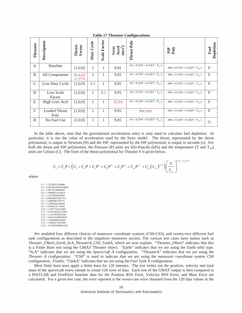
Table 17 Thruster ConfigurationsT

hrus

ter

Des

crip

tion

Thr

ust

Vec

tor

Dut

y C

ycle

Scal

e Fa

ctor

Gra

vA

ccel

(m/s

2 )

Thr

ust P

oly

ISP

Poly

Fuel

D

eple

tion

A Baseline (1,0,0) 1 1 9.8110 0.25 0.25( / )refP T T

300 0.25 0.25( / )refP T T Y

B All Components (x,x,x)x=.5774

1 1 9.81 10 0.25 0.25( / )refP T T 300 0.25 0.25( / )refP T T Y

C Low Duty Cycle (1,0,0) 0.1 1 9.81 10 0.25 0.25( / )refP T T 300 0.25 0.25( / )refP T T Y

D Low Scale Factor

(1,0,0) 1 0.1 9.81 10 0.25 0.25( / )refP T T 300 0.25 0.25( / )refP T T Y

E High Grav Acel (1,0,0) 1 1 12.14 10 0.25 0.25( / )refP T T 300 0.25 0.25( / )refP T T Y

F Loaded Thrust Poly

(1,0,0) 1 1 9.81 See text 300 0.25 0.25( / )refP T T Y

H No Fuel Use (1,0,0) 1 1 9.81 10 0.25 0.25( / )refP T T 300 0.25 0.25( / )refP T TN

In the table above, note that the gravitational acceleration entry is only used to calculate fuel depletion. In particular, it is not the value of acceleration used by the force model. The thrust, represented by the thrust polynomial, is output in Newtons (N) and the ISP, represented by the ISP polynomial, is output in seconds (s). For both the thrust and ISP polynomial, the Pressure (P) units are kilo-Pascals (kPa) and the temperature (T and Tref)units are Celsius (C). The form of the thrust polynomial for Thruster F is given below.

15 16

147 9 11

1

2

1 2 3 4 5 6 8 10 12 13

C C P

C PC C C

ref

TC C P C C P C P C P C P C P C C

Twhere

C1 = 1.23758251293888C2 = 0.00730193081644684C3 = 1.06710728099668C4 = 1.44084613514414C5 = 1.12975859384182C6 = 0.866449276427312C7 = 1.26090987550771C8 = 1.12890566239368C9 = 1.25439122773649C10 = 1.78577524273692C11 = 0.523539555272069C12 = 1.15120028332336C13 = 0.832532168870019C14 = 1.26666006242687C15 = 1.09502172813843C16 = -0.702022868622232

We modeled four different choices of maneuver coordinate systems (CS0-CS3), and twenty-two different fuel tank configurations as described in the impulsive maneuver section. The various test cases have names such as Thruster_FBurn_Earth_ScA_ThrusterA_CS0_TankA, which we now explain. “Thruster_FBurn” indicates that this is a Finite Burn test using the GMAT Thruster object. “Earth” indicates that we are using the Earth orbit type. “ScA” indicates that we are using the Spacecraft A configuration. “ThrusterA” indicates that we are using the Thruster A configuration. “CS0” is used to indicate that we are using the maneuver coordinate system CS0 configuration. Finally, “TankA” indicates that we are using the Fuel Tank A configuration.

Most finite burn tests apply a finite burn for 120 minutes. The test writes out the position, velocity and total mass of the spacecraft every minute to create 120 rows of data. Each row of the GMAT output is then compared to a MATLAB and FreeFlyer baseline data for the Position RSS Error, Velocity RSS Error, and Mass Error are calculated. For a given test case, the error reported is the worst-case error obtained from the 120 data values in the


output. The test case Thruster_FBurn_Earth_ScA_ThrusterA_CS0_TankA was the baseline test for the finite burn tests. In all the tests that follow, each test used the same configuration as the baseline test except for the one parameter that is varied in each table. The table of results below varies the orbit type. The position RSS difference ranged from approximately 1.1e-3 to 5.0e-2 m, the velocity RSS difference ranged from approximately 6.4e-7 to 7.7e-4 m/s, and the mass difference ranged from approximately 3.4e-6 to 1.1e-4 g.

Table 21 Orbit Type Results for Finite ManeuversOrbit Position RSS Error


(m/s)Mass Error

(g)Earth 2.644E-03 3.415E-06 1.547E-05

Jupiter 2.170E-02 1.066E-05 2.593E-05Luna 1.054E-02 3.728E-05 8.752E-05Mars 1.222E-03 1.195E-06 2.009E-05

Mercury 1.129E-03 2.450E-06 1.097E-05Neptune 2.791E-02 1.720E-05 2.417E-05

Pluto 5.000E-02 7.739E-04 1.098E-04Saturn 1.877E-03 6.404E-07 3.369E-06Uranus 7.388E-03 4.442E-06 1.211E-05Venus 1.198E-03 1.553E-06 5.555E-06

The table of results below varies the thruster configuration. The position RSS error ranged from approximately 3.0e-4 to 5.0e-3 m, the velocity RSS error ranged from approximately 3.8e-7 to 6.4e-6 m/s, and the mass error ranged from approximately 2.7e-8 to 2.4e-5 g. We note that the high gravitational acceleration thruster, which corresponds to a lower fuel mass flow rate, Thruster E, had the overall worst error. The thruster that did not model fuel use, Thruster H, had the lowest error.

Table 22 Thruster Configuration Results for Finite ManeuversThruster

ConfigurationPosition RSS Error


(m/s)Mass Error

(g)A 2.644E-03 3.415E-06 1.547E-05B 1.940E-03 2.421E-06 1.147E-05C 7.279E-04 7.070E-07 5.189E-07D 3.004E-03 2.922E-06 2.145E-05E 5.000E-03 6.436E-06 2.371E-05F 1.135E-03 1.080E-06 2.938E-07H 2.993E-04 3.802E-07 2.728E-08

The table of results below varies the maneuver coordinate system. The position RSS error ranged from approximately 2.3e-3 to 4.3e-3 m, the velocity RSS error ranged from approximately 2.2e-6 to 4.5e-6 m/s, and the mass error ranged from approximately 1.5e-5 to 3.0e-5 g.

Table 23 Maneuver Coordinate System Results for Finite ManeuversCoordinate System Position RSS Error


(m/s)Mass Error

(g)Earth Mean Equator J2000 (CS0) 2.644E-03 3.415E-06 1.547E-05

Earth VNB (CS1) 2.303E-03 2.169E-06 1.679E-05Earth LVLH (CS2) 4.338E-03 4.452E-06 2.994E-05

Attitude (CS3) 2.644E-03 3.415E-06 1.547E-05

The table of results below varies the tank configuration where we use the same tank configuration definitions used for the impulsive burn analysis. The position RSS error ranged from approximately 2.4e-4 to 9.7e-2 m, the velocity RSS error ranged from approximately 2.3e-7 to 7.7e-5 m/s, and the mass error ranged from approximately 3.5e-7 to 4.8e-3 g. The high mass blow down tank, Tank M, had the worst-case error for position, mass, and velocity. The pressure-regulated tank corresponding to Tank M, Tank B, had medium level errors. The low constant pressure tank, Tank D, had the least error for position, mass, and velocity.


Table 24 Tank Configuration Results for Finite ManeuversTank Configuration Position RSS Error


(m/s)Mass Error

(g)A 2.644E-03 3.415E-06 1.547E-05B 1.348E-03 1.709E-06 8.041E-06C 1.565E-03 2.855E-06 9.941E-06D 2.370E-04 2.312E-07 3.547E-07E 1.273E-03 1.651E-06 7.503E-06F 4.926E-03 6.360E-06 2.882E-05G 2.702E-03 3.489E-06 1.581E-05H 3.599E-03 4.660E-06 2.111E-05I 2.644E-03 3.415E-06 1.547E-05J 2.644E-03 3.415E-06 1.547E-05K 2.644E-03 3.415E-06 1.547E-05L 1.730E-03 1.977E-06 1.096E-05M 9.725E-02 7.728E-05 4.786E-03N 3.777E-03 5.065E-06 2.870E-05O 1.405E-03 1.367E-06 2.103E-06P 3.060E-03 3.507E-06 1.929E-05Q 5.681E-03 6.489E-06 3.537E-05R 3.642E-03 4.159E-06 2.287E-05S 2.423E-03 2.773E-06 1.536E-05T 4.402E-03 5.684E-06 2.577E-05U 9.262E-04 1.050E-06 5.981E-06V 1.838E-03 2.330E-06 1.089E-05

As shown in the table below, summarizing all finite burn maneuver results, the position RSS error ranged from approximately 2.4e-4 to 5.0e-2 m, the velocity RSS error ranged from approximately 2.3e-7 to 7.7e-4 m/s, and the mass error ranged from approximately 2.7e-8 to 4.8e-3 g.

Table 25 Summary of Finite Burn Maneuver ResultsTest Category Position RSS Error (m) Velocity RSS Error (m/s) Mass Error (g)

Low High Low High Low HighOrbit 1.1e-3 5.0e-2 6.4e-7 7.7e-4 3.4e-6 1.1e-4Thruster Configuration 3.0e-4 5.0e-3 3.8e-7 6.4e-6 2.7e-8 2.4e-5Coordinate System 2.3e-3 4.3e-3 2.2e-6 4.5e-6 1.5e-5 3.0e-5Tank Configuration 2.4e-4 9.7e-2 2.3e-7 7.7e-5 3.5e-7 4.8e-3All 2.4e-4 5.0e-2 2.3e-7 7.7e-4 2.7e-8 4.8e-3

We not that for most of the test cases above, for performance reasons, the numerical integration parameters were not set at the highest (most accurate) settings. For any particular test case, if increased accuracy was desired, better results could have been obtained by tightening up the numerical propagator tolerances. As expected, as a result of the finite vs. impulsive burn times and the corresponding increased numerical processing required for finite burns,the finite burn errors were larger than the impulsive burn errors.

V. Solvers Methodology and Results

The Solvers feature group includes the numerical algorithms, such as Differential Correction (DC) and Non-linear Programming (NLP), used to solve problems, as well as the commands needed for defining and controlling the simulation sequence. The types of numerical algorithms that GMAT uses to solve problems are broken up into two types, Targeters and Optimizers. Section A describes the Targeters testing methodology and results and Section B describes the Optimizers testing methodology and results.


A. Targeters

GMAT uses a single targeting method, a differential corrector (DC), to solve boundary value problems. When using the DC, the user specifies a choice of which algorithm to use (Newton-Raphson, Broyden, Modified Broyden) and which derivative method to use (forward, backward, and central difference). We tested and verified all permutations of these settings on both orbit dynamics and algebraic problem classes. For an orbit type problem, we verified that certain orbit related goals can be obtained within a desired tolerance. Examples of orbit parameter targets included B-plane components, semi-major axis, inclination, and velocity components. The orbit test cases utilized both impulsive and finite burns. The algebraic tests included solving the roots of a polynomial equation.

When using a DC, the user defines both the number of control variables (parameters that can vary) and the number of goals. A problem where the number of control variables equals the number of goals is called a ‘square’ problem. We tested the DC using both square and non-square problems.

We give an example test case below, showing the actual GMAT script syntax, where we use a finite burn along the spacecraft velocity component to achieve an orbit apogee of 12000 km. This is an example of a square problem as we have one control variable, the duration of a maneuver along the spacecraft velocity direction, and one goal, the desired orbit apogee radius value.

Create Spacecraft DefaultSC;Create Propagator DefaultProp;Create Thruster Thruster1;Thruster1.C1 = 1000; %defines thrust polynomial as constant at 1000 NThruster1.DecrementMass = true;Create FuelTank FuelTank1;Thruster1.Tank = {FuelTank1};Create FiniteBurn FiniteBurn1;FiniteBurn1.Thrusters = {Thruster1};DefaultSC.Tanks = {FuelTank1};DefaultSC.Thrusters = {Thruster1};Create Variable BurnDuration;Create DifferentialCorrector DC1;

BeginMissionSequence;

Propagate DefaultProp(DefaultSC) {DefaultSC.Earth.Periapsis};Target DC1;Vary DC1(BurnDuration = 200, {Upper = 10000});BeginFiniteBurn FiniteBurn1(DefaultSC);Propagate DefaultProp(DefaultSC){DefaultSC.ElapsedSecs=BurnDuration};EndFiniteBurn FiniteBurn1(DefaultSC);Propagate DefaultProp(DefaultSC) {DefaultSC.Earth.Apoapsis};Achieve DC1(DefaultSC.Earth.RMAG = 12000, {Tolerance = 1e-6});EndTarget;

Example 1 Target Finite Burn to Raise Apogee

GMAT scripting is based upon user-created objects. All of the commands before the BeginMissionSequence command define the objects needed for our analysis. Here, we have created a spacecraft, a fuel tank, a thruster, a propagator, a finite burn object, a differential corrector object, and finally a variable, BurnDuration, used to hold the length of our finite burn.

The first action after the BeginMissionSequence command is to propagate our spacecraft to perigee. The Target DC1 and Vary DC1(BurnDuration = 200, {Upper = 10000}) commands tell GMAT that we want to solve our problem using a DC process where our initial guess for the burn duration is 200 seconds. Next, we propagate our spacecraft to orbit apogee. Finally, the Achieve DC1(DefaultSC.Earth.RMAG = 12000, {Tolerance = 1e-6}) command tells GMAT that, as part of the DC process, we want our desired apogee radius value to be achieved within a 1e-6 km tolerance.


The script above converged to a burn duration value of 1213.19316046 seconds in six iterations and took 0.109 seconds to finish. The apogee radius value achieved differed from the target value by 6.955e-007 km, which is within our desired tolerance of 1e-6 km. For more details regarding the syntax used in this example, see the Target Finite Burn to Raise Apogee tutorial in the GMAT User Guide8.

B. Optimizers

GMAT allows you to solve optimization problems by using a NLP solver. Currently, you can choose from one of two available solvers, the fmincon solver object available to all GMAT users with access to the MATLABoptimization toolbox, and the VF13AD solver that can be built from source code available in the Harwell Subroutine Library. For the VF13AD solver, you can choose to use the forward or central derivative method. We tested all of these user options on sample problems. As was the case for the DC, we tested the optimizers on both orbit dynamics and algebraic type of problems. For an orbit type problem, we verified that certain orbit related quantities, such as fuel used or V , can be minimized while simultaneously constraining other orbit parameters. The algebraic problems included minimizing the height of a point constrained to lie on a circle.

We give an example test case below, showing the actual GMAT script syntax, where we use a VF13AD solver object to perform an impulsive burn to raise orbit apogee to a desired value. In this example, we have two control variables, the impulsive V to be applied in the spacecraft velocity direction and the true anomaly (TA) of where to perform the burn. For the goals, we have one quantity to be minimized and one quantity to be constrained. We want to minimize the V while simultaneously constraining the position vector magnitude at orbit apogee to 42164km to a 1 m tolerance.

Create Spacecraft aSat;

Create Propagator aPropagator;Create ImpulsiveBurn aBurn;Create VF13ad VF13ad1;VF13ad1.Tolerance = 1e-008;Create OrbitView EarthViewEarthView.Add = {Earth, aSat}EarthView.ViewScaleFactor = 5Create Variable ApogeeRadius DVCost;BeginMissionSequence;Optimize VF13ad1

Vary VF13ad1(aSat.TA = 100, {MaxStep = 10});Vary VF13ad1(aBurn.Element1 = 1, {MaxStep = 1});Maneuver aBurn(aSat);Propagate aPropagator(aSat) {aSat.Apoapsis};ApogeeRadius = aSat.RMAG;NonlinearConstraint VF13ad1(ApogeeRadius=42164,{Tolerance = 0.001);DVCost = aBurn.Element1;Minimize VF13ad1(DVCost);

EndOptimize;

Example 2 Optimize Impulsive Burn to Raise Apogee

As was previously discussed, GMAT scripting is based upon user-created objects. As such, all of the commands before the BeginMissionSequence command define the objects needed for our analysis. Here, we have created a spacecraft, a propagator, an impulsive burn, a VF13ad optimizer, and two variables, ApogeeRadius and DVCost, to hold the current values for apogee radius and V cost, respectively.

The first three commands after the BeginMissionSequence command setup the optimization problem. The Optimize VF13ad1 command tells GMAT that we will be performing optimization using the VF13ad1 solver object. The Vary VF13ad1(aSat.TA = 100, {MaxStep = 10}) command tells GMAT that the true anomaly where the burn is performed is a control variable with an initial value of 100 degrees. The Vary


VF13ad1(aBurn.Element1 = 1, {MaxStep = 1}) command tells GMAT that the impulsive V component along the spacecraft’s velocity vector is a control variable with an initial value of 1 km/s.

The next command propagates the spacecraft to orbit apogee and sets our user defined variable, ApogeeRadius,to the current value of the apogee radius. The next command NonlinearConstraintVF13ad1(ApogeeRadius=42164) tells GMAT that, as part of the optimization process, we have a goal of constraining the apogee radius to 42164 km within a 1 m tolerance. The next command sets the user defined variable, DVCost, to the current value of the control variable representing the impulsive V component along the spacecraft’s velocity vector. Finally, the Minimize VF13ad1(DVCost) command tells GMAT that, as part of the optimization process, we want to minimize the V applied.

The script above converged to a V value of 2.2431611641 km/s applied at a TA of -0.528860880875 degreesrequiring 24 iterations that were completed in 2.135000 seconds. As expected, the best ( V minimizing) orbit location to perform an apogee raising burn is near perigee (i.e., near TA = 0). In this example, since the force model in use in not perfectly a two body Keplerian, the optimal TA value obtained is close to but not exactly 0. The apogee radius achieved was within 5.43e-005 km of the desired value. For more details about the syntax used in this example, see the discussion of the Optimize Resource as well as the Optimal Lunar Flyby using Multiple Shootingtutorial in the GMAT User Guide8.

VI. Output and Utilities Methodology and Results

For the V&V program, GMAT’s Output and Utilities feature group contained the following features: orbit view, spacecraft visualization properties, ground track plot, xy plot, report file, and ephemeris file. Additionally, the group contained commands used to control output during the simulation process such as report, toggle, clear plot,mark point command, and pen up and pen down commands. In this paper, we only present test results for 2-Dgraphics, 3-D graphics, and ephemeris file. Although we present limited results in this paper, we performed extensive, systematic testing of all components found in Output and Utilities feature group. The last subsection describes at a high level the testing methodology that was used for other Output and Utilities features not presented in this paper.

A. 2-D Graphics

GMAT’s ground track plot is a 2-D graphics feature used to plot the longitude and latitude time-history for spacecraft. The V&V testing methodology for the ground track plot feature employed standard GMAT GUI testing plans and procedures. The first phase of testing involved visually inspecting each functional element of the ground track plot by the test engineer and either comparing graphical output to expected results in external tools or evaluating by using engineering judgment. For each element, the test engineer visually verified that ground track functionality performed as expected, and then prepared data for automated GUI regression testing for each ground track plot element. We considered testing complete when automated GUI tests were implemented by the GUI test engineer in the GUI regression test environment. Additionally, we implemented a suite of stress tests for this feature by writing tests that make heavy use of the graphical components during complex mission scenarios with numerous spacecraft displays.

GMAT supports 2-D xy data plots for graphical display of simulation data. The testing methodology for the xy plot feature used MATLAB as the external benchmark. We generated equivalent xy data plots in MATLAB and GMAT, and overlaid the plots to allow visual comparison of the graphical data. This comparison of the graphics from GMAT and MATLAB verified that the xy plot component accurately draws graphics on 2-D Cartesian axes.Similar to the ground track test procedures, we initially verified all xy plot functional elements and design requirements through visual inspection. Then, we implemented more rigorous and automated GUI testing of xy plot’s 2-D graphics by writing test scripts for each element. These test scripts were used by GUI test engineers tocreate screenshot images of the expected behavior for all graphical elements of xy-plot. These xy plot screenshots are used as the baseline truth data for GUI regression tests. Additionally, we conducted additional rigorous testing on xy plot functionality by writing stress tests designed to make excessive use of this feature.

B. 3-D Graphics


GMAT supports 3-D graphics used to visualize orbital trajectories of spacecraft and celestial bodies. Users candefine 3-D view properties such as the coordinate system, and view definition properties such as camera reference location and view directions. The 3-D graphics can optionally display coordinate system axes, constellations, xy or celestial planes, and the sun line. During iterative processes such as differential correction or optimization, orbit view provides the option to plot all perturbed trajectories or draw only the final converged trajectory.

We performed preliminary testing of 3-D graphics elements by visually inspecting the 3-D graphics behavior. We implemented more rigorous, automated GUI testing of the 3-D graphics by writing test scripts that automatically tested each orbit view functional element. The test scripts were used in GUI regression tests to automate the testing of 3-D graphics. Key elements of the graphics were verified by comparing GMAT’s 3-D graphics against Celestiaand STK benchmarks. Elements compared against external tools include drawing orbits, planes, sun-lines, stars, andconstellations. Additionally, we wrote stress test scripts designed make heavy use of 3-D graphics to ensure no graphics failures occur in those cases.

Figure 3 and Figure 4 illustrate the types of comparisons performed. Those figures illustrate the comparison of aspacecraft in a sun-centered trajectory (drawn in yellow), with ecliptic plane (shown in red), xy plane (blue), in the sun-centered mean J2000 axis system.

Figure 3 GMAT 3-D graphics output showing spacecraft trajectory, ecliptic plane, xy plane and sun-centered MJ2000Eq coordinate system


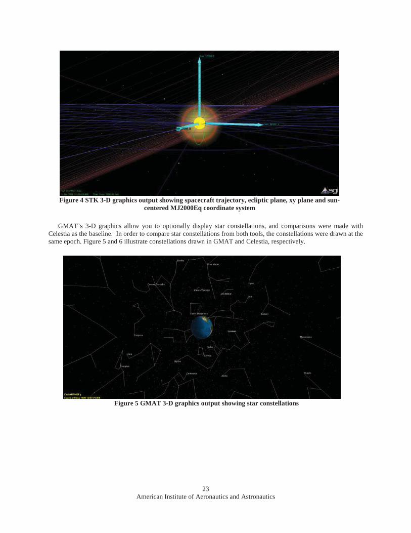
GMAT’s 3-D graphics allow you to optionally display star constellations, and comparisons were made with Celestia as the baseline. In order to compare star constellations from both tools, the constellations were drawn at the same epoch. Figure 5 and 6 illustrate constellations drawn in GMAT and Celestia, respectively.

Figure 5 GMAT 3-D graphics output showing star constellations

Figure 4 STK 3-D graphics output showing spacecraft trajectory, ecliptic plane, xy plane and sun-centered MJ2000Eq coordinate system


C. Ephemeris File

In GMAT R2013a, spacecraft orbit ephemeris data can be generated in either the standard Consultative Committee for Space Data Systems (CCSDS) or SPK file formats. The CCSDS ephemeris output is a standard ASCII text file while SPK ephemeris output is in binary format. Extensive, automated testing of the ephemeris file component was conducted through GMAT’s script test system. We wrote script tests for all functional elements ofthe ephemeris file feature. We compared interpolation to MATLAB and STK implementations for CCSDS ephemeris files and tested SPK ephemeris output by comparing the results to STK and the MICE toolbox.Additionally, we implemented stress tests that verify ephemeris output in simulations employing complex targeting and control flow.

D. Other Output and Utilities Components

The Output and Utilities feature group contained 11 components. In this paper, we only discussed the testing methodology for four of those components. The remaining 7 components went through equally rigorous and systematic testing during the V&V program. Table 26 contains brief descriptions of the testing methodology used for the remaining 7 components in the Output and Utilities group.

Figure 6 Celestia 3-D graphics output showing star constellations


Table 26: Test Methodology for Other Output and Utilities ComponentsComponent Test MethodologyReport File Tested reporting different data types such as user-defined variables, arrays, array elements,

strings, and parameters to report files. GMAT’s report file output was visually inspected for correctness. Those report files are used as baseline data in regression testing.

Report Command Tested reporting that different data types are correctly reported during the simulation when using the report command. GMAT’s report file output was visually inspected for correctness. Those report files are used as baseline data in regression testing.

Toggle Command

Tested toggle command on ReportFile and EphemerisFile subscribers through combination of both manual visual inspection and by creating baseline truth files using GMAT. Tested togglecommand on XYPlot, OrbitView and GroundTrackPlot by creating automated GUI tests which are included in GUI regression tests.

Spacecraft Visualization Properties

Tested spacecraft visualization properties primarily through manual visual inspection and also through automated GUI test system.

Clear Plot Tested clear plot command via the automated GUI test system and manual inspection.MarkPoint Tested mark point command via the automated GUI test system and manual inspection. PenUp/PenDown Tested pen up and pen down commands on the following subscribers: XYPlot, OrbitView and

GroundTrackPlot primarily through the automated GUI test system and manual inspection.

VII. Programming InfrastructureGMAT features extensive support for custom scripting of the mission sequence, a requirement to support the

complex needs of operational users. This support consists of a custom text-based script language along with a complement of data types, operators, interfaces, and components to enable users to implement complex sequences of events and perform mission-specific calculations. In the V&V program, the Programming Infrastructure component group consisted of the following components: numeric, array, and string variables; assignment and mathematics; mission data access; external interfaces to MATLAB; control flow; utility features such as named scripting environments and initialization; and the basic syntax and parsing of the script language itself. The V&V approach for all of these features can be divided into two major components: the script language and mission data calculation parameters.

A. Script Language

The goal of the script language V&V effort was to demonstrate that the various components that make up GMAT’s script language function as required and as expected when presented with both allowed and disallowed input. We divided the basic data types documented in the Script Language reference in the GMAT User Guide into the following basic classes of input:

1) literals: numeric, strings2) resources: variables, arrays, array elements, string variables, calculated parameters3) mathematical expressions

We tested each component of the script language with all applicable input types, in all permutations. For example, we tested setting a variable using numeric literals, array elements, other variables, spacecraft calculated parameters, etc. We tested setting and retrieving from arrays in multiple dimensions and at their size limits. For complex statements such as assignment and control flow (if, for, and while), we tested each syntax element (such as each logical operator argument) with all allowed input types. We followed this methodology for all components of the script language.

Additionally, we tested each functional element for proper behavior. For control flow statements, we tested each logical operator (and, or, not) in combination with all input types. We verified the behavior of the script environment by choosing a set of representative system tests and wrapped each in a script environment, making sure the output remained unchanged. For the external interface to MATLAB, we wrote tests that pass each input type to MATLAB


Table 18. Script language mathematical operators and functions.

Operators Functions+ (addition) sin exp - (subtraction) cos DegToRad * (multiplication) tan RadToDeg / (division) asin abs ' (transpose) acos sqrt ^ (power) atan norm atan2 det log inv log10

and then return it to GMAT, and then verify that the values are identical. We further tested the interface by calling different types of functions, including built-in, custom, and those with names that shadow existing names in GMAT.

GMAT’s assignment command fulfills two roles: assignment of one element to another (copying data), and performing mathematical calculations with a suite of built-in operators and simple functions. We verified the data assignment behavior by assigning each input type to each other input type and verifying that the data was copied correctly. We performed this step for each complex type (e.g. spacecraft, thruster) as part of the V&V program for that type. To test the mathematical role of the assignment command, we decomposed the syntax into the operators and functions shown in Table 18.

We tested each operator and mathematical function with each input data type and compared to either known results (for trivial calculations) or the output of the corresponding equation in MATLAB.

To test more complex expressions, we implemented a custom random mathematical expression generator in MATLAB. The generator builds an arbitrary random number of expressions of arbitrary random length from the component elements listed in Table 18, and with all variations of input data types. These equations are populated with sample data and evaluated in MATLAB to obtain a baseline value. Malformed equations and non-real results are discarded and replaced with new generated expressions. For added complexity, language-level elements are also added at random intervals, including whitespace and line-continuation characters. We applied this generator to create tests for the mathematical expression parser that included thousands of extremely complex equations, whichled to over a dozen issues being identified and fixed. Additionally, one hundred scripts, each with a random number of generated expressions, are run in the nightly regression testing process to maintain quality.

We tested the parsing of the script language itself by documenting every syntax element and testing each individually with a range of input types. Elements include comments, whitespace handling, literal data types (integers, real numbers, string literals, arrays), line-continuation characters, and allowed characters and character sets. We paid nearly equal attention to the graceful rejection of invalid input, including malformed syntax elements and unreadable files. We used random file generation to test GMAT for crashes on loading invalid files.

B. Mission Data Calculation ParametersOne of GMAT’s unique features as a mission analysis tool is its extensive and flexible data parameter

subsystem. GMAT contains many objects, like spacecraft, thrusters, maneuver models, etc. Each of these utilize properties that can be used to configure the objects, such as the spacecraft’s coefficient of drag, or the thruster’s Isp value. However, they also expose a set of output data parameters that can be calculated at the request of the user during the execution of the mission sequence. These include calculated quantities such as spacecraft altitude with respect to a central body, or the B-plane angle with respect to a targeting coordinate system. Often a property is both configurable and can be used as a calculated parameter; these include orbit state representation elements, such as semi-major axis. The semi-major axis of a spacecraft can both be set as an object property, or it can be calculated as a data parameter, often with respect to a different central body than that of the spacecraft itself. These dual-role parameters are called “read/write parameters.” Purely calculated parameters are called “read-only parameters.” The flexibility of the parameter subsystem is that certain parameters depend on either a celestial body (such as altitude) or a coordinate system (such as the B-plane vector). By specifying any available celestial body or coordinate system as the dependency, the parameter value is converted automatically. Examples of different parameters GMAT offers for certain objects are listed in Table 19.


We tested all read/write parameters, such as spacecraft state representations and thruster properties, as a part of the individual parent features in the V&V program, and we performed nominal testing here to confirm simple operation in an output context. For the numeric parameter-specific testing discussed here, we focused on read-only parameters, all of which are related to the spacecraft object.

We divided the full set of parameters into two classes: celestial-body dependent and coordinate-system-dependent. We tested both sets in a similar manner, by defining a set of reference orbits and calculating (and reporting) the value of each parameter in GMAT. We then defined identical reference orbits in the benchmark tools, and compared the reported values to a numeric tolerance. For the benchmark tools, we primarily used STK/Astrogator, and for trivial parameters, custom calculations implemented in MATLAB or GMAT’s script language. Table 20 and Table 21 summarize the cases tested and the numeric results.

Table 19: Examples of GMAT data parameters. Access is read/wrote (RW) or read-only (RO).Parameter Access DependencySpacecraftCartesian position RW Coordinate systemCartesian velocity RW Coordinate systemKeplerian elements RW Coordinate system,

celestial bodyEpoch RW (None)Attitude quaternion RW (None)Drag coefficient RW (None)Altitude RO Celestial bodyElapsed time RO (None)Orbit period RO Celestial bodyOrbital energy RO Celestial bodyB-plane parameters RO Coordinate systemState transition matrix RO (None)ThrusterDuty cycle RW (None)Thrust scale factorThrust polynomial coefficientsCartesian thrust vectorFuel tankFuel mass RW (None)Fuel densityTank volumeFuel pressureFuel temperatureImpulsive maneuverCartesian maneuver direction

RW (None)


All orbits are identical to those shown in Table 3. The state vectors for the additional Hyperbolic and Hyperbolic2 cases are shown in Table 22.

We judged the results shown here as acceptable to prove the accuracy of the parameter calculations for different orbit regimes and dependency values, and determined that the remaining error was caused by differences in modeling between the benchmark tool and GMAT.

Table 20 Selected test results for celestial-body-dependent calculated parameters. Benchmark tools are indicated as STK/Astrogator (AST), GMAT, and custom scripting implemented in each tool. Results are relative error between GMAT and the benchmark. A value of 1 indicates 100% error.

Orbit Celestial body

Altitude(AST)

Beta angle(cust. GMAT)

Orbit energy(cust. AST)

Mean motion(cust. AST)

Angular momentum(AST)

Velocity at periapsis(cust. AST)

GEO Earth 5e-12 < 1e-16 5e-14 8e-12 2e-11Venus 2e-12 2e-12 8e-11 6e-14 2e-11 4e-11

Hyperbolic Earth 3e-9 7e-15 6e-8 2e-11 2e-7 9e-8Venus 2e-11 3e-14 3e-8 1e-8 2e-8 2e-8

Mars Earth 2e-12 < 1e-16 3e-9 4e-9 2e-9 2e-9Mars 4e-8 < 1e-16 2e-9 2e-12 5e-10 5e-10

Luna Earth 2e-11 < 1e-16 5e-8 3e-14 9e-9 9e-9Luna 3e-9 < 1e-16 7e-10 6e-13 4e-10 4e-10

Table 22: Additional test cases for calculated parameters. States are relative to Earth J2000.Orbit Epoch X Y Z VX VY VZHyperbolic 01 Jun 2004

12:00 UTC12371.7915 5050.7627 5050.7627 -7.985992 2.445201 2.445201

Hyperbolic2 01 Jan 2000 12:00 TAI

-29840 0 -5463.8 4.1326 -3.787324 0.24139

Table 21: Selected test results for coordinate-system-dependent calculated parameters. STK/Astrogator was used as the benchmark tool in all cases. Results are relative error between GMAT and the

benchmark. A value of 1 indicates 100% error.Orbit Coordinate

systemVelocity magnitude

RAAN Declination Right ascension of velocity

Right ascension of hyperbolic asymptote

Declination of hyperblic asymptote

GEO Earth J2000 4e-12 5e-14 5e-14 2e-9Saturn Fixed 8e-12 2e-5 8e-13 2e-5

Hyperbolic Earth J2000 3e-8 1e-13 4e-9 4e-9Saturn Fixed 6e-13 2e-6 7e-13 2e-5

Hyperbolic2 Earth J2000 7e-8 3e-8Saturn Fixed 7e-8 4e-8

Mars Mars J2000 5e-9 2e-11 2e-5 9e-7Saturn Fixed 6e-13 6e-6 3e-13 6e-6

Luna Moon J2000 5e-10 6e-13 2e-6 3e-7Saturn Fixed 4e-13 3e-6 4e-13 2e-5


Figure 7 GATS Test Driver Interface

VIII. GUI Testing

The goal of the GMAT GUI testing effort was, and is, to provide complete test coverage for GMAT. We neededto ensure 100% coverage of the GUI (every button, every text box, every menu, etc. gets tested at least once) and 100% requirements fulfillment (every GUI-related requirement is fulfilled by the GUI). Most importantly, GUI testing had to be automatable and repeatable. Testing the GUI once every release cycle or even once a month was not acceptable. To ensure consistent quality, GMAT GUI regression testing needed to happen as automatically and hopefully almost as often as script testing.

The GMAT project uses SmartBear Software’s TestComplete to perform automated GUI testing on Windows platforms. TestComplete allows users to easily create, maintain, and execute automated tests for exercising the widgets of their GUI. It allows the GMAT GUI Test Team to perform functional and regression testing of the GMAT GUI.

A. Methodology

For GMAT, we divided the GUI tests into 2 different types: “unit” tests and system tests. Unit tests ensure verification and acceptance testing of every button, menu, text box, etc. for complete coverage of the GMAT GUI and GMAT GUI requirements. Every unit test project exercises one object (resource, command, script window, mission sequence, etc) in the GMAT system and its specific GUI. System tests seek to validate the GMAT GUI by testing the entire application using end-to-end test cases by simulating typical end-user interactions with the systemwith the intent of qualifying GMAT as a fully functional application.

The GMAT script test team is aggressive in performing regression testing frequently to catch new errors early and as they happen. For GMAT 2013a, we performed the full suite of script tests nightly. This process had been automated and in place for years (though it grew significantly during the V&V program). The goal of the GMAT GUI test team was to perform GUI regression testing in a similar manner. After selection of SmartBear’s TestComplete, it took over a year to develop a full suite of GUI unit and system tests. Even though it is easy to create GUI tests with TestComplete, it is labor intensive to create good, maintainable tests. Initial efforts made it clear that we needed to refactor how we developed GUI unit tests. The re-factorization efforts paid off - with the use of new templates, we were able to generate much more robust unit tests in a fraction of the time. Due to schedule factors, refactoring of GUI System tests did not occur until after the R2013a release. While the System tests performed well and provided much needed GUI testing while we developing the GUI unit tests, they required a lot of manual intervention.


Figure 8 GATS Sample Test Results

Figure 9 Sample GUI System Test Tracking

We developed an automated GUI test execution tool, the GMAT Automated Test Suite (GATS), to automate the execution of the GUI unit tests (and eventually GUI System tests), map tests to requirements, and report results.GATS ingests a requirements-to-test matrix (RTTM) spreadsheet, executes every test, saves the recorded results, and provides analysis help. Figure 7 shows a sample GATS RTTM. GMAT testers used GATS to analyze results, re-execute failed tests, associate bugs with tests (to be able to track expected failures in the future), and report GUI Regression test results to the GMAT team.

GATS significantly reduced GUI regression test effort and analysis. In January 2012, it took approximately 14 days to manually execute and analyze 53 Unit test projects (totaling approximately 1000 tests). By March 2013, GATS was autonomously executing 90 GUI unit test projects (totaling approximately 3400 tests) in 4 days, requiring only 1-2 days of manual analysis (a 10x reduction in effort while providing 3.4x the coverage). GMAT developers had the primary responsibility to analyze regression reports and address test regressions due to code modifications and additions. If analysis indicated a regression appeared to be the result of a poorly designed or flawed test, then it was the responsibility of test analysts to modify the test accordingly.

B. Results

For GMAT 2013a, the GUI System testing was performed semi-automatically 1.3 times per week and was in place early to help identify software issues. After the release of GMAT R2012a in May 2012, we were executing 38 system tests in a 2-hour period. By 2013a, we were executing a total of 45 system tests in a 3-hour period. Figure 9 shows the GUI system testing results in the final year before release.As you can see, GUI System testing helped us track bug fixes and immediately see failures such as the failure spike for the November 6th,2012 build.

We also had a baseline for GUI Unit Regression testing in place in May 2012 with 1650 tests. The first baseline took 6 days to run as we had to reruntests continuously to get everything working smoothly, even with use of GATS. We gave ourselves a goal of performing GUI Unit testing every 2-4 weeks based on that experience.

Over the R2013a development cycle, we continually improved the unit test suite and reduced the time to perform unit regression testing (See Figure 9). By the time of the GMAT 2013a release, we performed GUI Unit Regression testing every 1 to 2 weeks, which is remarkable considering we had almost doubled the number of tests. By March, GUI Unit testing automatically executed 2937 tests in approximately 77 hours.

Proper GUI testing is a matter of continuous improvement. Since GMAT R2013a, we have continued to improve our GUI testingprocesses. GMAT GUI Unit Testing now includes over 3400 individual tests executedautomatically every weekend (taking approximately 70 hours). Since it is not feasible to execute the full suite of GUI unit tests nightly, we selected 400 tests as a representative subset of the full suite to execute nightly as a GUI Smoke test. In addition, GMAT GUI System testing are now completely refactored and automated. We execute 109 GUI System tests nightly; it takes approximately 11 hours. The combination of the GUI System tests and the GUI Unit Smoke tests gives us a nightly regression test giving acceptable confidence in the daily GMAT build. In a related effort, we automated every GMAT GUI tutorial, allowing us to catch interface changes between releases that might break the user tutorials.


Figure 10 Sample GUI Unit Test Tracking

GMAT GUI testing has been a remarkable success. GMAT’s GUI is the best tested (and retested) application that the GMAT team has ever developed in their careers for NASA. It provides a significant complement to the large nightly script test suite to enable our customers’ confidence in GMAT’s quality.

IX. ConclusionThis paper documents the verification and validation of GMAT resulting in version R2013a, the first Gold

version of the software. The V&V program began in the winter of 2012, after GMAT had been in Beta form for approximately 5 years and used extensively as a preliminary design tool. As of the completion of the V&V effort, GMAT was rigorously tested on the Windows 7 platform, and nightly regression tests included approximately 13,000 test scripts and approximately 3400 automated GUI tests.

We achieved all technical and programmatic goals of the effort:

Systematically evaluated and validated all models, components, and functionalityFixed nearly all critical system defectsUpdated working specifications that define system behaviorProvided high quality end user documentation and training materialPrepared for system maintenance and further development of a NASA Class B flight qualified systemPositioned GMAT for larger community adoption Positioned GMAT for flight qualification

We consider GMAT to be the best tested (and retested) system that we have encountered in our work for NASA.As evidence, we presented high-level test results in most system areas, and detailed test results for key areas. For key numeric areas such as dynamics and modelling, coordinate systems, and numerical integration, we presented results showing excellent agreement with industry-standard baseline systems. As of the time of writing, R2013a has received approximately 6000 downloads of the Windows application files, an approximately 50% increase from the equivalent time before the V&V program. The GMAT V&V effort continues to pay dividends and has withstood constant expansion and revision. The GMAT R2013a V&V effort led to a smooth follow-on effort for flight qualification, described by Qureshi1, resulting in version R2013b, the first flight qualified version of GMAT.

References

1Qureshi, Rizwan, and Hughes, Steven, P., “Preparing the General Mission Analysis Tool for Operational Maneuver Planning of the Advanced Composition Explorer Mission (ACE).” AIAA/AAS Astrodynamics Specialist Conference, San Diego, CA, 2014, (submitted for publication).

2MATLAB, Software Package, Version R2013a, Mathworks, Natick, MA, 2013.3Test Complete, Software Package, Version 9.3, SmartBear, Beverly, MA, 2013.4STK, Satelite Tool Kit, Software Package, Version 8.1.3 and 9.2.3, Analytical Graphics, Inc., Exton, PA, 2008. 5FreeFlyer, Software Package, Version 6.7.2, a.i. solutions, Lanham, MD, 2012.6Celestia, Software Package, Version 1.6.1, Celestia Development Team, 2010.


7Vallado, David, A. “An Analysis of State Vector Propagation Using Differing Flight Dynamics Programs”, AAS/AIAA Space Flight Mechanics Conference, 2005.

8GMAT, General Mission Analysis Tool, Software Package, Version R2013a, NASA Goddard Space Flight Center, Greenbelt, MD, 2013.

9Hughes, Steven, P. “GMAT Software Management Plan (SMP)”, NASA Goddard Space Flight Center, Greenbelt, MD, 2013.

10Grubb, Thomas, G., “GMAT Test Plan”, NASA Goddard Space Flight Center, Greenbelt, MD, 2013.


verification and validation of the general mission ... · verification and validation of the...

Documents