verificacion del principio ergodico para un …€¦ · differential superposition expression: u d...

Aqua-LAC - Vol. 4 - Nº.1 - Mar. 2012 19

VERIFICACION DEL PRINCIPIO ERGODICO PARA UN PROCESO DE DISPERSION EN FLUJOS.

VERIFICATION OF ERGODIC PRINCIPLE FOR A DISPERSION PROCESS IN FLOw.

Alfredo Constaín Aragón1

Resumen

Se presenta en este artículo un análisis de las condiciones por medio de las cuales es alcanzado aproximadamente el equilibrio Termodinamico en el ancho de un flujo natural. En este momento también puede ser aplicado el bien conocido “Principio Ergodico” llevando a conocer cuando un soluto vertido al flujo se extiende casi homogéneamente en la sección transversal del mismo. Esta es la condición de “Mezcla completa”, muy importante para estudios de contaminación y de calidad del agua. También es discutida la aplicación de este desarrollo a un par de experimentos con trazadores en un gran rio de montaña y un pequeño arroyo en Colombia. Aunque los razonamientos expuestos son termodinámicos en naturaleza, las conclusiones y las ecuaciones derivadas pueden ser aplicadas con facilidad en la Ingeniería. PALAbRAS CLAVE: Trazadores, Longitud de mezcla, estudios de contaminación.

Abstract

It is presented in this article an analysis of conditions by means of which thermodynamic equilibrium is approximately reached across the wide of a natural flow. In this moment also it may be applied the well known” ergodic principle” leading to know when a poured solute is spread almost homogeneously on cross section of flow. This is the “Complete mixing” condition, very important for contamination and quality of water studies. Also it is discussed the application of this devel-opment to a couple of practical tracer experiments in a large mountain river and in a small stream in Colombia. Although the reasoning exposed is thermodynamic in nature, the conclusions and derived equations may be applied quite well to Engineering. KEywORDS: Tracers, Mixing length, contamination studies.

1. I+D Manager, Amazonas Technologies, Cali, Colombia [email protected]

Artículo enviado el 8 de noviembre de 2011Artículo aceptado el 19 de julio de 2012

INTRODUCTION

The fact that most of real human level processes are all irreversible gives a special character to those physical events: Thermodynamics allow describing them in a simple and comprehensive way with a sur-prisingly small degree on details of process (Meyer, 1982) This is especially true for a key totally irrevers-ible phenomenon as Diffusion of solutes in water flow-ing. Then it is possible to use some thermodynamics concepts to develop a useful approach to calculation of the so-called “Complete mixing condition” in which conservative tracer has dispersed in all cross section of flow.

STREAM MEAN VELOCITy AND DISPERSION VELOCITy OF A TRACER.

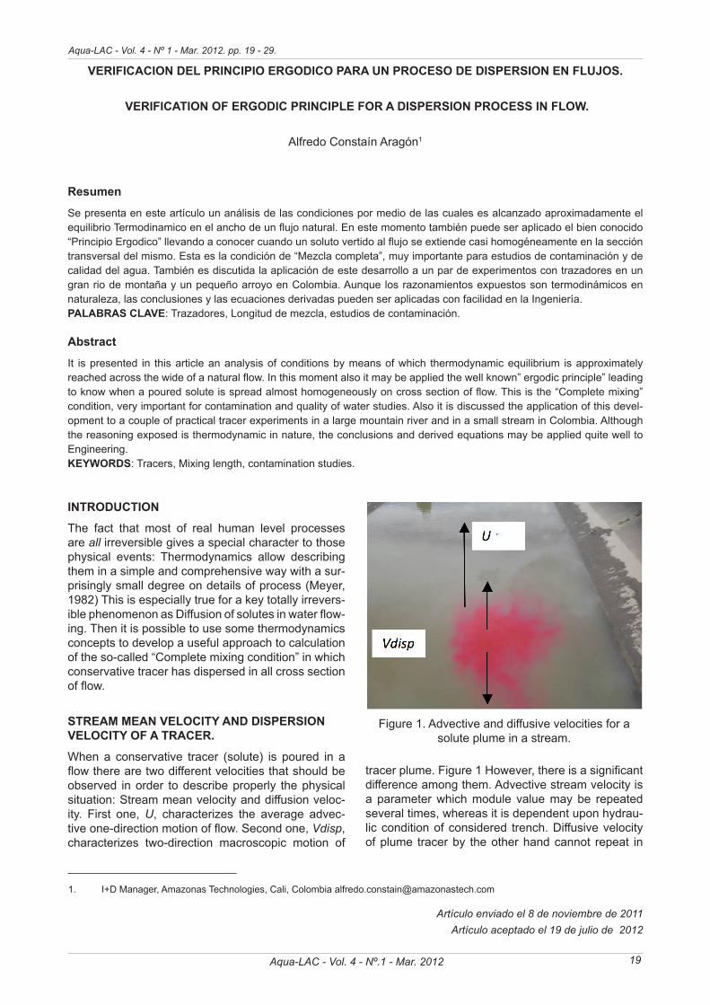
When a conservative tracer (solute) is poured in a flow there are two different velocities that should be observed in order to describe properly the physical situation: Stream mean velocity and diffusion veloc-ity. First one, U, characterizes the average advec-tive one-direction motion of flow. Second one, Vdisp, characterizes two-direction macroscopic motion of

Figure 1. Advective and diffusive velocities for a solute plume in a stream.

tracer plume. Figure 1 However, there is a significant difference among them. Advective stream velocity is a parameter which module value may be repeated several times, whereas it is dependent upon hydrau-lic condition of considered trench. Diffusive velocity of plume tracer by the other hand cannot repeat in

Aqua-LAC - Vol. 4 - Nº 1 - Mar. 2012. pp. 19 - 29.

20

Alfredo Constain Aragon

Aqua-LAC - Vol. 4 - Nº.1 - Mar. 2012

module value because is a characteristic of irrevers-ible diffusion process. When the chemical equilibri-um is broken due to pouring, a specific mechanism should appear to restore it accord with Le Chatelier principle (Prigogine, Kodepudi, 1998) so diffusion ve-locity is the way in which the tracer tends to spread toward equilibrium as last stage. Then U velocity is not a state function while Vdisp has this nature. How-ever, there is a certain relationship among them. An increase of advective velocity should lead generally to an increase of dissipative factors (by means of tur-bulence generated by roughness) and then to a dif-ferent pattern of diffusion velocity, then it is possible to define a state function, Φ, at constant temperature and pressure, in the following way (Constain, 2011a) (Constain, 2011 b):

UVdisp=φ

(1)

It is interesting to develop a specific definition of this function. First one may define a characteristic dis-placement of diffusion (one variance), Δ using the Brownian one-dimension model, with τ correspond-ing characteristic time and E the Longitudinal disper-sion coefficient.

τE2=∆

(2)

As Nobel Prize winner I. Prigogine (Prigogine, 1997) had pointed out extensively studying Poincare´s chaotic processes, this model is more general than usually is taken because not only free (thermal) in-dependent molecular motions are Brownian but also potentially (dependent) molecular motions evolve (transmitting disorder) with same law. Now, Vdisp may be defined as:

τ∆=diffV

(3)

Hence:

τφEU 21=

(4)

Clearing Φ function in this equation and putting it as differential superposition expression:

dUU

dEE

d

∂∂+

∂∂= φφφ

(5)

Using Eq (4) it is easy to verify that dΦ is an exact differential accordingly with following equation:

∂

∂∂

=

∂

∂∂

UE

EU

φφ

(6)

And then:

∫ =C

d 0φ

(7)

That is, Φ is a state function as was defined before, and it describes thermodynamic evolution of plume from dissipation point of view in the same way that Chezy´s coefficient, C, characterizes friction effect in uniform flow regime, as function of energy line slope, S, and hydraulic radio, R.

RSCU =

(8)

Here it is interesting to see how the two equations for mean velocity of flow have same structure, following Occam´s principle in the sense that Nature does not multiply entities describing same thing.

AN APPROACH TO IRREVERSIbLE EVOLUTION OF TRACER PLUME IN FLOw.

When a closed system (which don’t interchange mass with its environment) evolves with temperature and pressure constant there is a function that describes thermodynamic evolution of the system: Gibbs po-tential, G (Zemansky, 1967).This function represents the part of enthalpy (forma-tion heat in Hess´s scheme) that can be converted in work and then its curve defines the evolution of available energy within system in such way that its decrement –ΔG indicates how initial energy, ΔH is spent until equilibrium is reached. Figure 2

Figure 2. Tracer plume Energy evolution in flow.

Verification of ergodic principle for a dispersion process in flow

21Aqua-LAC - Vol. 4 - Nº.1 - Mar. 2012

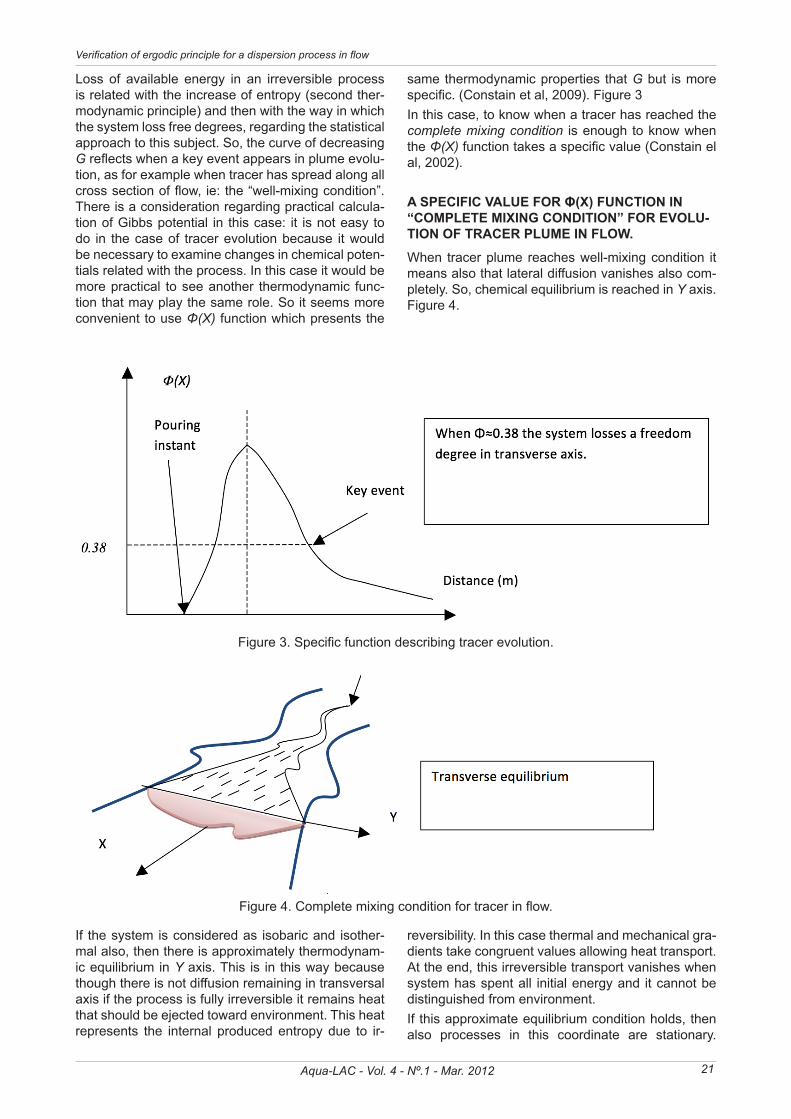
Loss of available energy in an irreversible process is related with the increase of entropy (second ther-modynamic principle) and then with the way in which the system loss free degrees, regarding the statistical approach to this subject. So, the curve of decreasing G reflects when a key event appears in plume evolu-tion, as for example when tracer has spread along all cross section of flow, ie: the “well-mixing condition”. There is a consideration regarding practical calcula-tion of Gibbs potential in this case: it is not easy to do in the case of tracer evolution because it would be necessary to examine changes in chemical poten-tials related with the process. In this case it would be more practical to see another thermodynamic func-tion that may play the same role. So it seems more convenient to use Φ(X) function which presents the

Figure 3. Specific function describing tracer evolution.

same thermodynamic properties that G but is more specific. (Constain et al, 2009). Figure 3In this case, to know when a tracer has reached the complete mixing condition is enough to know when the Φ(X) function takes a specific value (Constain el al, 2002).

A SPECIFIC vALuE FOR Φ(X) FunCTIOn In “COMPLETE MIXInG COnDITIOn” FOR EvOLu-TION OF TRACER PLUME IN FLOw.

When tracer plume reaches well-mixing condition it means also that lateral diffusion vanishes also com-pletely. So, chemical equilibrium is reached in Y axis. Figure 4.

Figure 4. Complete mixing condition for tracer in flow.

If the system is considered as isobaric and isother-mal also, then there is approximately thermodynam-ic equilibrium in Y axis. This is in this way because though there is not diffusion remaining in transversal axis if the process is fully irreversible it remains heat that should be ejected toward environment. This heat represents the internal produced entropy due to ir-

reversibility. In this case thermal and mechanical gra-dients take congruent values allowing heat transport. At the end, this irreversible transport vanishes when system has spent all initial energy and it cannot be distinguished from environment. If this approximate equilibrium condition holds, then also processes in this coordinate are stationary.

22



Hence here is possible to apply the well know ergod-ic principle to the system. This principle has several versions whereas is one of most fertile in physics. One of them very useful to the faced problem is pre-sented in the following way (Pugachev, 1973): For a steady random variable, Y(x), the mean value is constant, then the outcomes for different argument values: Y(x1),Y(x2)....,Y(Xn) and the outcomes for different functions with the same argument: Y1(x), Y2(x)....,Yn(x) are equivalent, leading for the same mean value. Figure 5.This principle means that when tracer has reached well-mixed condition there are two different concentrations that are convergent, be-ing useful to know the key value for Φ(X) function in Mixing Length, Φo. To apply this approach is conve-nient to define first set of concentration along all vol-ume of tracer where concentrations are peak values for different X coordinate. Figure 5. Second set may be defined conveniently as different concentrations (function of Y coordinate) in a specific distance, Xo, where is the peak value.Figure 6

Figure 5. Concentration distribution based on first set.

Figure 6. Concentration distribution based on sec-ond set.

If we extent the calculation to a infinite number of val-ues for two sets, it states as follows:

n

xCnC n

np

x

∑∞→=

)(lim

(9)

And

∫=lim

0lim

)(1 Y

y dyyCy

C

(10)

It is easy to see that firsts mean concentration along all plume is:

o

x tQMC×

≈

(11)

Here M is the tracer mass poured in injection point (considering conservative solute), Q the discharge of

flow and to be the time spent from injection point to Mixing length.For second mean concentration is necessary to use error function to integrating the expression. Here y lim is a characteristic value of transverse coordinate related to inflection points of Gaussian bell form.

poy CC ×≈ 441.0

(12)

Here Cpo is peak concentration value in Xo, the Mix-ing Length. Hence, using ergodic principle:

xy CC ≈

(13)

This means that:

poo

CtQ

M ×≈×

441.0

(14)

Now, to relating this expression with Φ(Xo) it is nec-essary to use a modified Fick´s equation. This equa-tion results from the replacement of relationship (4) in classical one (15a), Here A is cross section of flow.

tEtUX

etEA

MtxC 4

2)(

4),(

−−=π

(15a)

Therefore,

2222

2)(

2),(

tU

tUX

etQMtxC βφ

πβφ

−−

×××= (15b)

Here β≈0.215 from Poisson´s analysis of plume evo-lution. Then, peak value for well-mixed condition is:

o

o



16.1×××≈

oopo tQ

MCφ

(16)

Replacing Eq (16) in Eq (14) it states:

38.016.1441.0 ≈≈oφ

(17)

This result means that, in every case, tracer plume spreads along cross section of flow when Φ takes the approximate value 0.38.

5. A COMPARISON OF DEVELOPED SPECIFIC VALUE OF Φo FUNCTION FOR “COMPLETE MIXInG COnDITIOn” AnD RuThvEn´S RELA-TIONSHIP.

In a science field, when a new formula is developed one of first requirements is that its results being con-vergent with well accepted formulas. Then new ap-proach should be compared with a well established relationship. Unfortunately due to huge spread of semi empirical formulas about tracer theory, there is not a unique, wide accepted one. However, an ap-proximate definition for Mixing Length due to Ruth-ven has been very used along the years with satis-factory results:

yo

WUXε

2

075.0 ×≥ (18)

Here W is the mean transverse distance (wide) of flow and εy the transverse diffusion coefficient. Now, this equation is for a centerline injection; for an injec-tion at the side of stream width has to be multiply by two and coefficient to be multiplied by 4, remaining:

yso

WUXε

2

3.0 ×≥ (19)

To analyze the issue is necessary to write concentra-tion distribution in transverse coordinate as follows.

ty

yye

tQMCtyC ε

φ4

)( 2

16.1),(

−

== (20)

It should be noted that we use Cp value as is defined in Eq (15) due to continuity principle between longi-tudinal and transversal functions. Now, clearing the value for transverse diffusion coefficient and reorder-ing factors:

ty

CtQ

M

Ln

y

Y

4

16.1

1 2

×

××

×

=

φ

ε (21)

For well-mixed condition in which there is thermo-dynamic equilibrium in Y axis, tracer concentration value may be replaced by more probable value which in turn is the mean value, accord with Darwin-Fowler principle in statistical mechanics (Morowitz, 1971).

poyy CCC 441.0≈≈

(22)

Then

( ) tW

CC

Ln

y

op

p 4

16.1441.0441.01 2

×

×××

=

φ

ε (23)

Hence:

tW

Lny

416.138.0

11 2

×

×

=ε (24)

And, replacing time by key distance divided by veloc-ity

oXWUy

422.1

2××≈ε (25)

Finally:

yo

WUXε

2

305.0 ××≈ (26)

This result is very close to Ruthven´s equation for side injection.

SOME CONSIDERATION AbOUT FUNCTION Φ(X).

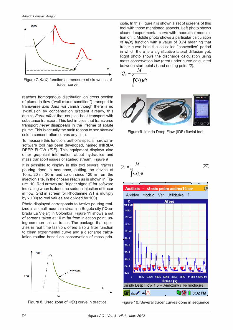
Beside the thermodynamic considerations discussed in this article about Φ(X) there are some characteris-tics of this function that deserve our attention. First, if it is accepted that skewness of tracer curves in real life is due to a kinematic composition (Galilean trans-formation) between one-direction mean flow velocity and two-direction diffusion velocity, then ratio of these two kind of velocities is a measure of the observed skewness. Figure 7.Upper curve shows a higher degree of skewness corresponding to a higher value of Φ(X) function. Lower curve by the other hand has a lower degree of skewness, corresponding to a lower value of func-tion. Second, experimental values of Φ(X) have been encountered as high as 0.8 and low as 0.15 in tracer measurements done by author. Third, always is used decreasing edge (green line) of function curve. In practice never has been used other zone of it. Figure 8. There is another important remark to do at this point regarding the key value of Φ(Xo)≈0.38. Once solute

o

24



Figure 7. Φ(X) function as measure of skewness of tracer curve.

reaches homogenous distribution on cross section of plume in flow (“well-mixed condition”) transport in transverse axis does not vanish though there is no Y-diffusion by concentration gradient already, this due to Foret effect that couples heat transport with substance transport. This fact implies that transverse transport never disappears in the lifetime of solute plume. This is actually the main reason to see skewed solute concentration curves any time. To measure this function, author´s special hardware-software tool has been developed, named INIRIDA DEEP FLOW (IDF). This equipment displays also other graphical information about hydraulics and mass transport issues of studied stream. Figure 9It is possible to display in this tool several tracers pouring done in sequence, putting the device at 10m., 20 m, 30 m and so on since 120 m from the injection site, in the chosen reach as is shown in Fig-ure 10. Red arrows are “trigger signals” for software indicating when is done the sudden injection of tracer in flow. Grid in screen for Rhodamine WT is multiply by x 100(so real values are divided by 100).Photo displayed corresponds to twelve pouring real-ized in a small mountain stream in Bogota city (“Que-brada La Vieja”) in Colombia. Figure 11 shows a set of screens taken at 10 m far from injection point, us-ing common salt as tracer. The package that oper-ates in real time fashion, offers also a filter function to clean experimental curve and a discharge calcu-lation routine based on conservation of mass prin-

Figure 8. Used zone of Φ(X) curve in practice.

ciple. In this Figure it is shown a set of screens of this tool with those mentioned aspects. Left photo shows cleaned experimental curve with theoretical modela-tion on it. Middle photo shows a particular calculation of Φ(X) function with a value of 0.74 meaning that tracer curve is in the so called “convective” period in which there is a significative lateral diffusion yet. Right photo shows the discharge calculation using mass conservation law (area under curve calculated between start point t1 and ending point t2).

Figure 9. Inirida Deep Flow (IDF) fluvial tool

∫= 2

1

)(t

t

a

dttC

MQ (27)

Figure 10. Several tracer curves done in sequence



There is also in the middle photo a warning label in Spanish indicating that key value Φ≈ 0.38 is not reached yet and that injection distance has to be en-larged.

Figure 11. IDF screens shown filter, modelation and calculation routines.

Figure 12. Experimental usage of hardware-software IDF tool in a small stream.

Some aspects of measurement task are shown in Figure 12 Experiment is done on a small stream of 0.042 m3/s of discharge and a mean flow velocity of 0.11 m/s.

26



Figure 13 shows the Φ(X) curve for all twelve pour-ing experiments in the trench of 120 m with a mean width W of 1.5 m This information was downloaded from memory of IDF tool. In this curve it is observed, according with theory explained in this Article that well-mixed condition for tracer plume is about 72 m distance in which Φ(X) ≈0.38 as key value.EXPERIMEnTAL vERIFICATIOnS OF “ERGODIC COnDITIOnS” AT Φ(Xo) ≈0.38 RELATIONSHIP.

Small mountain stream (“Quebrada la vieja”).

As a representative example of these verifications fol-lowing is shown experiment at X=70 m for a journey in the small stream documented before. Selection of this particular result is obvious because mixing length is supposed about 72 m and then in this case the numerical values may be applied to verify theoretical conjectures. Tracer poured mass was 200 grams of NaCl ionic. Data download from IDF tool for this par-ticular experiment is in Table 1.

Data Value

M 200 grms

Xo 70 m

Cpo 16.9 mgr/l

U 0.120 m/s

Q 0.0450 m3/s

Qa 0.0443 m3/s

to 583.3 s

Figure 13. Φ(X) curve for a 12 tracer pouring experiments.

Фo 0.39

W 1.5 m

Table 1. Data for experiment in “Quebrada La vieja”.

It should be noted in data of this Table that discharge calculated using Fick´s modified equation, Q, and mass conservation principle, Qa, are very close nu-merically with a relative error less than 1%. Now, the ergodic principle applied to specific condi-tions of this small stream in Table 1 holds:

lMgrssl

MgrtQ

M

o

/26.73.58/45

200000≈

×=

× lMgrlMgrC po /45.7/9.16441.0441.0 ≈×=×

Then key concentrations differs one to each other in a relative error less than 3%. This means that already for X≈70 m. there is well-mixed condition for tracer in considered flow. This event occurs at Ф≈0.39 very close to key value of 0.38 as was stated in theoretical developments.

Large mountain river (“Rio Cali”).

Author´s research team had worked several field jour-neys between 2005 and 2009 to test ergodic principle applied to tracer plume evolution using IDF tool (Am-azonas Tech, 2009). Among them there was a case lying in “complete mixing” condition that is studied herein. Tracer used in this occasion was Rhodamine



WT. Some aspects of that measurement journey are shown in Figure 14. This is a stream located in Cali city at southwest of Colombia in the day of measurements this river has a discharge approximately of 4.8 m3/s and a mean velocity of 0.76 m/s. This trench of this stream is one

Figure 14. Author´s team at the border of “Rio Cali” stream using IDF tool

of a typical mountain river with large slope and rough-ness and meanders with 25 m wide in average.Next are presented the screens of IDF tool for three slug (sudden) experiments done at a distance of 613 m. and with two values of tracer mass. First tracer injection is done with 10 grams and second and third with 4 grams. Left upper photo shows tracer curve

Figure15. IDF screens with graphical information of first curve and function Φ1(X=613 m)

with original noise. Middle photo shows action of IDF filter cleaning noise spikes and right upper photo shows theoretical modelation using equation (15b) overimpossed on real curve. Lower photo shows Φ function measured at X=613 m.

1.- First pouring with 10 grams of Rhodamine WT. Figure 15 2. - Second pouring with 4.0 grams of Rhodamine WT.

Figure 16. IDF screens with graphical information of second curve and function Φ2(X=613 m)

28



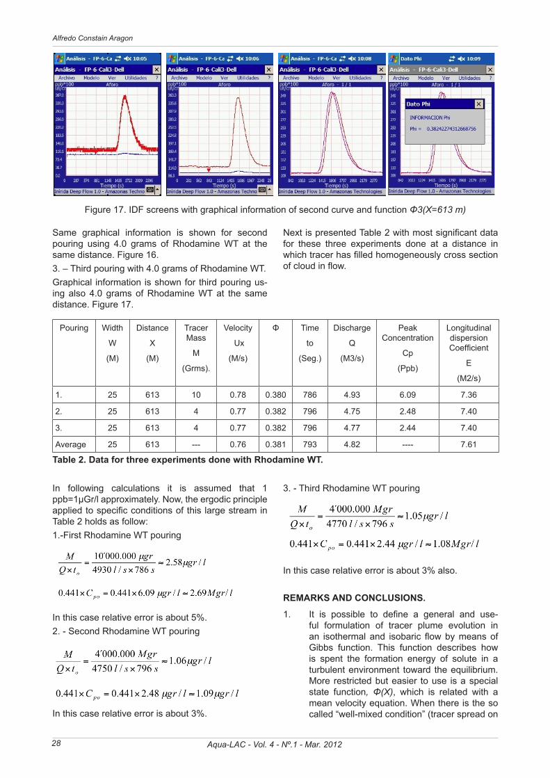
Same graphical information is shown for second pouring using 4.0 grams of Rhodamine WT at the same distance. Figure 16.3. – Third pouring with 4.0 grams of Rhodamine WT.Graphical information is shown for third pouring us-ing also 4.0 grams of Rhodamine WT at the same distance. Figure 17.

Figure 17. IDF screens with graphical information of second curve and function Φ3(X=613 m)

Next is presented Table 2 with most significant data for these three experiments done at a distance in which tracer has filled homogeneously cross section of cloud in flow.

Pouring Width

W

(M)

Distance

X

(M)

Tracer Mass

M

(Grms).

Velocity

Ux

(M/s)

Φ Time

to

(Seg.)

Discharge

Q

(M3/s)

Peak Concentration

Cp

(Ppb)

Longitudinal dispersion Coefficient

E

(M2/s)

1. 25 613 10 0.78 0.380 786 4.93 6.09 7.36

2. 25 613 4 0.77 0.382 796 4.75 2.48 7.40

3. 25 613 4 0.77 0.382 796 4.77 2.44 7.40

Average 25 613 --- 0.76 0.381 793 4.82 ---- 7.61

Table 2. Data for three experiments done with Rhodamine WT.

In following calculations it is assumed that 1 ppb=1μGr/l approximately. Now, the ergodic principle applied to specific conditions of this large stream in Table 2 holds as follow: 1.-First Rhodamine WT pouring

lgrssl

grtQ

M

o

/58.2786/4930

000.000´10µ

µ≈

×=

× lMgrlgrC po /69.2/09.6441.0441.0 ≈×=× µ

In this case relative error is about 5%.2. - Second Rhodamine WT pouring

lgrssl

MgrtQ

M

o

/06.1796/4750

000.0004́µ≈

×=

× lgrlgrC po /09.1/48.2441.0441.0 µµ ≈×=×

In this case relative error is about 3%.

3. - Third Rhodamine WT pouring

lgrssl

MgrtQ

M

o

/05.1796/4770

000.0004́µ≈

×=

× lMgrlgrC po /08.1/44.2441.0441.0 ≈×=× µ

In this case relative error is about 3% also.

REMARKS AND CONCLUSIONS.

It is possible to define a general and use-1. ful formulation of tracer plume evolution in an isothermal and isobaric flow by means of Gibbs function. This function describes how is spent the formation energy of solute in a turbulent environment toward the equilibrium. More restricted but easier to use is a special state function, Φ(X), which is related with a mean velocity equation. When there is the so called “well-mixed condition” (tracer spread on



all cross section of flow) this function has the value 0.38.This approach is convergent with classical 2. ones, as for example Ruthven´s empirical equation. Using the condition Фo≈0.38 is pos-sible to obtain Mixing Length, Xo.Current methods usually limit two different 3. stages in tracer evolution: “Convective” period in which there is significative transverse dif-fusion and “Diffusive” period in which only is longitudinal dispersion. First period occurs in earlier moments of plume transport and cur-rently is supposed that tracer curves are much skewed, lacking a formal representation in Gaussian form. Within the theory presented by author, it is assumed that this kind of asymme-try is not a real but a virtual effect, which allow accepting this kind of curves like Gaussian in every moment. The Ergodic principle which is the foundation 4. of new method is examined for two different streams, finding that this condition for “Mixing length” is convergent with experimental re-sults.Presented methodology allows to do critical 5. solute fate studies since in current procedures it is not possible to interpret plume evolution, avoiding to get a very important information on water quality methods.

bIbLIOGRAPHIC REFERENCES.

Amazonas Technologies (2009), Fomipyme project, final report (internal circulation).Bogota, Colombia (Non published).

Constain A., Agredo O., Carvajal J. (2002). Applica-tions of a new mean flow velocity equation in streams. River Flow, Lovaine la neuve.

Constain A., Carvajal ACarvajal., J. (2009). Accurate measurement of discharge using Rhodamine WT. IAHR Intl. Congress, Vancouver.

Constain A., (2011a) Svedber´s number playing a main role in diffusion processes. (to be published) European Physics Journal.

Constain A.. (2011b) Is storage mechanism in Dead Zone model violating second principle? (to be publis-hed) European Physics Journal.

Meyer R. (1982) , Introduction to mathematical fluid dynamics. Dover publications, New York.

Morowitz H.J. (1971). Entropy for biologist: An intro-duction to thermodynamics. Academic Press, New York.

Prigogine I., Kondepudi D. (1998). Modern Thermo-dynamics. Jhon Wiley & Sons. New York.

Prigogine I. (1997). El fin de las certidumbres. Tau-rus, Bns As.

Pugachev V.S. (1973). Introduction to Probability the-ory. Nauka Editors, Moscow.

Zemansky M.W. (1967), Heat and thermodynamics. Mc Grw-Hill, New York.

verificacion del principio ergodico para un …€¦ · differential superposition expression: u d...

Documents