verbal information veriflcation for high-performance ... · verbal information veriflcation for...
TRANSCRIPT

Verbal Information Verification for
High-performance Speaker Authentication
Qin Chao
A Thesis Submitted in Partial Fulfillment
of the Requirements for the Degree of
Master of Philosophy
in
Electronic Engineering
c©The Chinese University of Hong Kong
June 2005
The Chinese University of Hong Kong holds the copyright of this thesis.
Any person(s) intending to use a part or whole of the materials in the thesis
in a proposed publication must seek copyright release from the Dean of the
Graduate School.

To my loving family

Acknowledgements
First of all, I am grateful to my supervisor, Prof. Tan Lee, for having guided
me with an open but practical mind, for introducing me the interesting topic
of speech processing, for inspiring me on writing research papers, and for his
generous support to my Ph.D study. I thank Prof. P.C Ching and H.T Tsui for
writing supportive reference letters for me, Prof. Helen Meng for her biometric
project which gave me the opportunity to study in CUHK, Prof. X.G Xia for
encouraging me in my application interview, Dr. Frank Soong for sharing me his
brilliant insights into machine learning, and Prof. Y.T Chan for his marvellous
course on advanced DSP.
Special thanks are given to Mr. K.F Chow for sharing with me his many
great ideas on speech recognition and for his great RSBB framework, and Miss
M.T Cheung for the happy time with her.
During two years, I have sought helps from friends and colleagues that have
helped me in many ways. C. Yang, Y. Qian, N.H Zheng, Y.Y Tam, Patgi Kam,
S.W Lee, Y.C Chan, L. Tsang, W. Zhang, L.Y Ngan, Y.J Li, Y. Zhu, S.L Oey,
Dexter Chan, and H. Ouyang help me a lot academically.
And technical support from Mr. Arthur Luk is much appreciated.
iii

Abstract of thesis entitled:
Verbal Information Verification for High-performance
Speaker Authentication
Submitted by QIN Chao
for the degree of Master of Philosophy
in Electronic Engineering
at The Chinese University of Hong Kong in
June 2005.
Automatic speaker authentication is to authenticate the identity of a claimed
speaker by verifying the identity-related information embedded in his/her spo-
ken utterances. The information mainly refers to the voice characteristic and
the verbal content. This leads to two closely related technologies. One is speaker
verification (SV) and the other is verbal information verification (VIV).
Throughout this thesis, speaker authentication is studied for users who speak
Cantonese. A SV system has been developed using state-of-the-art techniques
with digit-based contexts. The universal background model (UBM) adaptation
method are adopted and compared with the Cohort method. In VIV, many con-
siderations in the process of constructing anti-models, e.g., the way of pooling
subword units, the model structure and the model complexity, are discussed. A
new technique is proposed to provide more reliable and effective anti-likelihood
scores. Our method uses the Gaussian Mixture Model (GMM) instead of the
conventional Hidden Markov Model (HMM) for anti-modeling at the subword
level. Three methods for integrating SV and VIV systems are investigated.
They are voting method, support vector machines (SVMs) and Gaussian-based
classifier respectively.
Experiments on 20 Cantonese speakers show that for SV the best result with
equal error rate (EER) of 1.5% can be attained using the UBM adaptation.
For VIV the experimental results indicate that the proposed GMM-based anti-
iv

models constructed using combined Cohort-and-World methods exhibit the best
separation between the true utterance and the erroneous one. The best result
is obtained with EER equals to 0.45%. Error-free performance is achieved by
using the Gaussian-based classifier to integrate two systems.
v

摘 要
自動説話人認證是透過辨認嵌入于語音中的身份信息來確認説話人的身份。與身
份相關的信息主要包括說話人的語音特徵和語音内容。籍此而產生說話人確認和
語義信息確認兩种相關技術。
本論文主要研究廣東話自動説話人認證技術。我們利用最新的技術實現了一個基
於數字文本的說話人確認系統。在該系統中,我們採用了通用背景模型適應技術
並與傳統技術進行了比較。在開發語義信息確認技術過程中,我們詳加考察了訓
練反模型的方法,例如字詞的聚類、模型的結構與複雜度問題,並提出一種新技
術。我們在字詞級別用高斯混合模型取代了傳統的隱馬爾科夫模型。本文還嘗試
了三种不同方法用於結合這兩种系統。它們分別是表決法、支持向量機和高斯分
類器。
說話人確認系統實驗表明通用背景模型適應技術性能最優。語義信息確認實驗指
出我們提出的反模型建模方法性能優良,能夠有效將正確與錯誤語句分離。最後,
基於高斯分類器,自動説話人認證系統可達零錯誤率。

Contents
1 Introduction 1
1.1 Overview of Speaker Authentication . . . . . . . . . . . . . . . . 1
1.2 Goals of this Research . . . . . . . . . . . . . . . . . . . . . . . 6
1.3 Thesis Outline . . . . . . . . . . . . . . . . . . . . . . . . . . . . 7
2 Speaker Verification 8
2.1 Introduction . . . . . . . . . . . . . . . . . . . . . . . . . . . . . 8
2.2 Front-End Processing . . . . . . . . . . . . . . . . . . . . . . . . 9
2.2.1 Acoustic Feature Extraction . . . . . . . . . . . . . . . . 10
2.2.2 Endpoint Detection . . . . . . . . . . . . . . . . . . . . . 12
2.3 Speaker Modeling . . . . . . . . . . . . . . . . . . . . . . . . . . 12
2.3.1 Likelihood Ratio Test for Speaker Verification . . . . . . 13
2.3.2 Gaussian Mixture Models . . . . . . . . . . . . . . . . . 15
2.3.3 UBM Adaptation . . . . . . . . . . . . . . . . . . . . . . 16
2.4 Experiments on Cantonese Speaker Verification . . . . . . . . . 18
2.4.1 Speech Databases . . . . . . . . . . . . . . . . . . . . . . 19
2.4.2 Effect of Endpoint Detection . . . . . . . . . . . . . . . . 21
2.4.3 Comparison of the UBM Adaptation and the Cohort
Method . . . . . . . . . . . . . . . . . . . . . . . . . . . 22
2.4.4 Discussions . . . . . . . . . . . . . . . . . . . . . . . . . 25
2.5 Summary . . . . . . . . . . . . . . . . . . . . . . . . . . . . . . 26
3 Verbal Information Verification 28
3.1 Introduction . . . . . . . . . . . . . . . . . . . . . . . . . . . . . 28
vi

3.2 Utterance Verification for VIV . . . . . . . . . . . . . . . . . . . 29
3.2.1 Forced Alignment . . . . . . . . . . . . . . . . . . . . . . 30
3.2.2 Subword Hypothesis Test . . . . . . . . . . . . . . . . . . 30
3.2.3 Confidence Measure . . . . . . . . . . . . . . . . . . . . . 31
3.3 Sequential Utterance Verification for VIV . . . . . . . . . . . . . 34
3.3.1 Practical Security Consideration . . . . . . . . . . . . . . 34
3.3.2 Robust Interval . . . . . . . . . . . . . . . . . . . . . . . 34
3.4 Application and Further Improvement . . . . . . . . . . . . . . 36
3.5 Summary . . . . . . . . . . . . . . . . . . . . . . . . . . . . . . 36
4 Model Design for Cantonese Verbal Information Verification 37
4.1 General Considerations . . . . . . . . . . . . . . . . . . . . . . . 37
4.2 The Cantonese Dialect . . . . . . . . . . . . . . . . . . . . . . . 37
4.3 Target Model Design . . . . . . . . . . . . . . . . . . . . . . . . 38
4.4 Anti-Model Design . . . . . . . . . . . . . . . . . . . . . . . . . 38
4.4.1 Role of Normalization Techniques . . . . . . . . . . . . . 38
4.4.2 Context-dependent versus Context-independent Anti-
models . . . . . . . . . . . . . . . . . . . . . . . . . . . . 40
4.4.3 General Approach to CI Anti-modeling . . . . . . . . . . 40
4.4.4 Sub-syllable Clustering . . . . . . . . . . . . . . . . . . . 41
4.4.5 Cohort and World Anti-models . . . . . . . . . . . . . . 42
4.4.6 GMM-based Anti-models . . . . . . . . . . . . . . . . . . 44
4.5 Simulation Results and Discussions . . . . . . . . . . . . . . . . 45
4.5.1 Speech Databases . . . . . . . . . . . . . . . . . . . . . . 45
4.5.2 Effect of Model Complexity . . . . . . . . . . . . . . . . 46
4.5.3 Comparisons among different Anti-models . . . . . . . . 47
4.5.4 Discussions . . . . . . . . . . . . . . . . . . . . . . . . . 48
4.6 Summary . . . . . . . . . . . . . . . . . . . . . . . . . . . . . . 49
5 Integration of SV and VIV 50
5.1 Introduction . . . . . . . . . . . . . . . . . . . . . . . . . . . . . 50
5.2 Voting Method . . . . . . . . . . . . . . . . . . . . . . . . . . . 53
vii

5.2.1 Permissive Test vs. Restrictive Test . . . . . . . . . . . . 54
5.2.2 Shared vs. Speaker-specific Thresholds . . . . . . . . . . 55
5.3 Support Vector Machines . . . . . . . . . . . . . . . . . . . . . . 56
5.4 Gaussian-based Classifier . . . . . . . . . . . . . . . . . . . . . . 59
5.5 Simulation Results and Discussions . . . . . . . . . . . . . . . . 60
5.5.1 Voting Method . . . . . . . . . . . . . . . . . . . . . . . 60
5.5.2 Support Vector Machines . . . . . . . . . . . . . . . . . . 63
5.5.3 Gaussian-based Classifier . . . . . . . . . . . . . . . . . . 64
5.5.4 Discussions . . . . . . . . . . . . . . . . . . . . . . . . . 66
5.6 Summary . . . . . . . . . . . . . . . . . . . . . . . . . . . . . . 67
6 Conclusions and Suggested Future Works 68
6.1 Conclusions . . . . . . . . . . . . . . . . . . . . . . . . . . . . . 68
6.2 Summary of Findings and Contributions of This Thesis . . . . . 70
6.3 Future Perspective . . . . . . . . . . . . . . . . . . . . . . . . . 71
6.3.1 Integration of Keyword Spotting into VIV . . . . . . . . 71
6.3.2 Integration of Prosodic Information . . . . . . . . . . . . 71
Appendices 73
A A Cantonese VIV Demonstration System 73
Bibliography 77
viii

List of Tables
2.1 Statistics of the Digit Corpus of CUCALL . . . . . . . . . . . . 20
2.2 Statistics of the Digit Corpus of CUSV . . . . . . . . . . . . . . 20
4.1 Cantonese Sub-syllable Clustering based on Confusion Matrix . 41
4.2 Cantonese Sub-syllable Clustering based on K-means Clustering 42
4.3 Comparisons of training time of different anti-models (Training
were carried out on a PC with Pentium 4 processor) . . . . . . . 43
4.4 Statistics of the Sentence Corpus of CUCALL . . . . . . . . . . 46
5.1 Results using voting method with shared thresholds . . . . . . . 61
5.2 Results obtained with the combined system on individual thresholds 62
ix

List of Figures
1.1 An example of verbal information verification process (after [1]). 3
1.2 Speaker authentication approaches (after [1]) . . . . . . . . . . . 4
1.3 The system by combining VIV with speaker verification (after [1]) 5
2.1 Modular representation of the training phase of a speaker verifi-
cation system (after [9]). . . . . . . . . . . . . . . . . . . . . . . 9
2.2 Modular representation of the testing phase of a speaker verifi-
cation (after [9]). . . . . . . . . . . . . . . . . . . . . . . . . . . 9
2.3 Modular representation of a filterbank-based cepstral parameter-
izations [9]). . . . . . . . . . . . . . . . . . . . . . . . . . . . . . 10
2.4 Likelihood-ratio-based speaker verification (after [9]). . . . . . . 14
2.5 Pictorial example of two steps in adaptation of a hypothesized
speaker model (after [17]) . . . . . . . . . . . . . . . . . . . . . 17
2.6 Illustration of the effect of endpoint detection in speaker verification 22
2.7 A typical waveform used in our experiment . . . . . . . . . . . . 23
2.8 Comparison of verification performance based on the Cohort
method with different number of mixture components . . . . . . 24
2.9 Comparison of verification performance based on UBM adapta-
tion with different number of mixture components . . . . . . . . 25
3.1 Utterance verification approach to VIV. . . . . . . . . . . . . . . 29
x

3.2 Histograms for the utterance-level scores for two classes. One
class of data is from clients and the other class of data is from
impostors. From top left to bottom right: (a) using averaged
target likelihood scores without likelihood ratio test, (b) using
CM1 confidence measure, (c) using CM2 confidence measure (d)
using CM3 confidence measure . . . . . . . . . . . . . . . . . . . 33
3.3 False acceptance rate as a function of robust interval for a 0%
false rejection rate. . . . . . . . . . . . . . . . . . . . . . . . . . 35
4.1 Illustration of manual alignment compared with state-of-the-art
automatic alignment on the utterance “baat-saam-gau-jat-ng-
baat-sei-jat-jat-jat”, each panel shows, from top to bottom: (a)
the waveform, (b) the spectrogram, (c) time axis (d) the manual
alignment, and (e) the automatic alignment . . . . . . . . . . . 39
4.2 Equal Error Rate vs. Model Complexity . . . . . . . . . . . . . 46
4.3 Equal Error Rate vs. Weighting factor α in combined Cohort-
and-World (C&W) anti-models . . . . . . . . . . . . . . . . . . 47
4.4 Comparisons of system performance based on various context-
independent anti-models. . . . . . . . . . . . . . . . . . . . . . . 48
5.1 Histogram for the SV likelihood scores for two classes. One class
is from client data and the other one is from impostor data. No
single threshold value will serve to unambiguously discriminate
between the two classes. . . . . . . . . . . . . . . . . . . . . . . 51
5.2 Histogram for the VIV likelihood scores for two classes. One class
is from client data and the other one is from impostor data. No
single threshold value will serve to unambiguously discriminate
between the two classes. . . . . . . . . . . . . . . . . . . . . . . 51
5.3 Scatter plot of VIV scores vs SV scores. The dark line could serve
as a decision boundary of our classifier. . . . . . . . . . . . . . . 52
5.4 Structure of the integrated authentication system . . . . . . . . 53
xi

5.5 Example of the criteria for taking the values of the thresholds
when FA and FR curves cross . . . . . . . . . . . . . . . . . . . 55
5.6 Example of the criteria for taking the values of the thresholds
when FA and FR curves do not cross . . . . . . . . . . . . . . . 56
5.7 Linear separating hyperplanes for the separable case. The sup-
port vectors are circled. (after Burges [45]) . . . . . . . . . . . . 58
5.8 False acceptance and false rejection rates obtained using the vot-
ing method with shared thresholds. β varies between 0 and 1 . . 61
5.9 False acceptance and false rejection rates using the voting method
with individual thresholds. β varies between 0 and 1 . . . . . . 62
5.10 The learned decision boundary of SVMs and scatter plot of the
development data . . . . . . . . . . . . . . . . . . . . . . . . . . 63
5.11 The learned decision boundary and scatter plot of the evaluation
data . . . . . . . . . . . . . . . . . . . . . . . . . . . . . . . . . 64
5.12 The learned decision boundary of GMM-based classifier and scat-
ter plot of the development data . . . . . . . . . . . . . . . . . . 65
5.13 The learned decision boundary of GMM-based classifier and scat-
ter plot of the evaluation data . . . . . . . . . . . . . . . . . . . 66
A.1 Main interface of VIV system . . . . . . . . . . . . . . . . . . . 74
A.2 Sample question . . . . . . . . . . . . . . . . . . . . . . . . . . . 74
A.3 The detailed interface . . . . . . . . . . . . . . . . . . . . . . . . 75
A.4 The task grammar used in keyword spotting . . . . . . . . . . . 75
xii

Chapter 1
Introduction
Authentication of personal identity is an essential requirement for controlling
access to protected resources. Traditionally, personal identity is usually claimed
by presenting a unique personal possession such as a key, a badge, a password or
a signature. However, these can be lost, stolen, or counterfeited, thereby posing
a threat to security. Furthermore, a simple identity claim might be insufficient
if the potential loss is great. Penalty for false acceptance is necessary.
Recently, human authentication by biometrics receives great attention as it
can provide convenience to users while maintaining a high degree of security.
Biometric authentication can be regarded as a practical application of pattern
classification, where the goal is to authenticate the identity of users by measuring
their physical traits, like iris, face, lips, palm print, voice, fingerprint, etc. Apart
from these physiological characteristics, the users’ behavior also provides cues
to idiosyncrasy. These biometric features can be used to discriminate among
individuals for two reasons. First, it is well known that every one is born
individually. Second, these features normally remain invariant over a fairly long
term.
1.1 Overview of Speaker Authentication
Among these biometrics, voice is the most convenient one in that it is easy to
produce, capture and transmit for remote processing. The process of confirming
1

Chapter 1. Introduction
a speaker’s identity by his/her speech is referred to as speaker authentication
(SA). How to extract discriminative identity-related information from the speech
signal is a crucial problem in the research on speaker authentication [1].
If the decision is made on the physical characteristics of voices, the task is
named speaker recognition. It has been studied for several decades. Since mid-
90’s, NIST 1 has united researchers around the world to work on various practical
problems in speaker recognition. With the continuous research efforts and the
advances in computing technology, significant progress has been made in the
past decade, making it possible to transfer the research results from laboratory
simulation to real-world applications. There are however still many problems
that affect the reliability, security and user-friendliness of authentication system,
such as acoustic mismatch, quality of training data, the inconvenience of user
enrollment, and the creation of large databases to store the speaker models [1].
As an enhancement to the speaker authentication technology, a novel ap-
proach called verbal information verification (VIV) was proposed [2]. It requires
the user to speak out his/her personal information such as name, birth date and
residential address in order to verify the identity. Different kinds of questions
can be asked to implement different security levels, which could be used for
users with different levels of authorities when accessing a system. The opera-
tion of an example VIV system is illustrated as in Fig. 1.1. It is similar to a
typical telephone-banking procedure: after an account number is provided, the
operator verifies the user by asking some personal information, such as mother’s
maiden name, birth date, mobile number, address, etc. The user can only gain
access into to his/her account only if the questions are answered correctly. To
automate the whole verification procedure, the questions can be prompted by
either a text-to-speech system (TTS) or using pre-recorded messages.
VIV can be used independently or combined with speaker verification system
to provide the convenience to users, meanwhile a higher level of security could
be achieved.
1National Institute of Standards and Technology (NIST) is the federal technology agency
that works with industry to develop and apply technology, measurements, and standards.
2

Chapter 1. Introduction
“In which year were you born?”
Get and verify the answer utterances.
Get and verify the answer utterance.
“In which city/state did you grow up?” Rejection
“May I have you telephone number, please?”
Get and verify the answer utterances.
Rejection
Rejection
Acceptance on 3 utterances
Figure 1.1: An example of verbal information verification process (after [1]).
In the following discussion, speaker authentication refers to the process of
authenticating a user via his/her voice input using pre-stored information. The
information can be in various formats, such as lexical transcriptions, acoustic
models, text, subword sequence, etc [1]. As shown in Fig. 1.2, speaker authenti-
cation can be categorized into two groups: by the speaker’s voice characteristics
as in conventional speaker recognition, or by the content of an utterance as in
verbal information verification. Speaker recognition could be further divided
into speaker identification (SID) and speaker verification (SV). SID is the pro-
cess of associating an utterance with a member in a pool of known speakers. It
can be referred to as many to one mapping. SV is the process of verifying the
claimed identity of an unknown speaker by comparing the voice characteristics
as encapsulated in spoken input against a pre-stored speaker-specific model. It
is a binary decision problem.
A speaker recognition system needs an enrollment session to collect data for
the training of speaker-specific models. The enrollment causes inconvenience
to users as well as the system developers who have to supervise the process
of data collection. The quality of training data is critical to the performance
3

Chapter 1. Introduction
Speaker Authentication
Speaker Recognition
(Authentication by
voice characteristics)
Verbal Information Verification
(Authentication by
verbal content)
Speaker
Identification
Speaker
Verification
Figure 1.2: Speaker authentication approaches (after [1])
of a SV system. However, it might be too demanding and unrealistic to ex-
pect the users pronounce all training utterances correctly. Furthermore, since
the training and testing voices may come from different transmission channels
or acoustical environments, SV systems suffer from the acoustic mismatch be-
tween the training and testing conditions. The mismatch significantly affects
the system performance.
On the other hand, VIV only needs speaker-independent statistical models
to associate acoustic events with phonetic identities. During enrollment, only
the user’s personal profile in text format is needed. A user’s personal data
profile is created when the user’s account is set up. VIV doesn’t require a
lengthy enrollment process and suffers less from acoustic mismatch. Since no
speaker-specific voice characteristics are used in the verification process, it is
solely the user’s responsibility to protect his/her own information. Once these
information are known by others intentionally, system security can not be guar-
anteed. Therefore, in practical application, we have to devise many ways to
avoid impostors using the speaker’s personal information by monitoring a par-
ticular session. As in [1], a VIV system can ask for some information that are
not constant from time to time, e.g., the amount or date of the last deposit; or
a subset of the registered personal information, e.g., a VIV system can require
a user to register N piece of personal information (N > 1), and each time only
randomly ask n questions (1 ≤ n < N). Furthermore, a VIV system can be
migrated to a SV system after speaker-specific utterances for enrollment are
collected. This approach is shown in Fig. 1.3, where VIV is involved in the
4

Chapter 1. Introduction
enrollment and one of the key utterances in VIV is the pass-phrase which will
be used in SV later. During the first 4 − 5 accesses, the user is verified by a
VIV system. The verified pass-phrase utterances are recorded and later used
to train an speaker-dependent HMM for SV. At this point, the authentication
process can be switched from VIV to SV.
VerbalInformationVerification
VerbalInformationVerification
Speaker Verification
Speaker Verification
HMM Training
HMM Training
Automatic Enrollment
Save of training
Pass-phrase for the first few accesses
Identity claimTest pass-phrase:“Open Sesame”
Database
Score
“Open Sesame”………
………
SD HMM
Speaker Verifier
Verified passphrases fortraining
Figure 1.3: The system by combining VIV with speaker verification (after [1])
Suppose that we are going to design a security log-in system for restricted
access to some confidential files in a computer using the technique of speaker
authentication. Only those registered users are allowed to browse or download
the files. The approach described above provides a desirable solution because
of several advantages of the combined system. First, the approach is convenient
to users since it does not need a formal enrollment session and a user can start
to use the system right after his/her account is opened. Second, the acoustic
mismatch problem maybe mitigated since the training data are from different
sessions. Third, the quality of the training data are ensured since the training
phrases have been verified by VIV before they are used in speaker modeling.
Finally, once the system switches to SV, it will be rather difficult for an impostor
to access the account even if the true speaker’s phrase is known by an impostor.
Also, we may not have to use the two system sequentially. That is, VIV can
be also used in the operation instead of only being used in enrollment session.
There are several types of impostors:
• Naive impostor whose voice is unlike the true speaker and without knowing
the pass-phrases.
5

Chapter 1. Introduction
• Impostor who knows all pass-phrases but his voice is very different from
the true speaker.
• Impostor whose voice is very close to the true speaker but without knowing
any of pass-phrases.
• Impostor whose voice is very like the true speaker while knowing some of
the pass-phrases.
In order to deal with the first type of impostors, either SV or VIV alone would
be sufficient to reject them. For the second type of impostors, SV alone can
reject them rightly. For the third type of impostors, VIV alone can reject them
correctly. For the last type of impostors, if the impostor was asked for only some
questions with fixed order, even combined use of SV and VIV might not be able
to reject them. However, if questions to be asked were selected randomly from
the question pool, this type of impostors could be rejected.
1.2 Goals of this Research
In speaker authentication, the normalization technique plays a vital role in
determining the performance of an authentication system. The performance is
known to be significantly affected by the variation of the signal characteristics
from trial to trial.
In speaker verification, the modeling of background speakers has been found
to affect the system performance significantly. Many research efforts have been
made to testify this importance. Despite the lack of a theoretical interpreta-
tion on the requirements for optimal background models, a number of effective
techniques have been proposed [3][4][5].
Anti-modeling plays a similar role in VIV to background speaker modeling
in SV. It provides a normalization score in likelihood ratio test and makes the
normalized likelihood score be more stable and less variable, thus leading to
improved performance. Some researches were conducted on anti-modeling in
VIV [6][7][8]. However, there has been little systematic work seriously focused
6

Chapter 1. Introduction
on the design of anti-models. This is the focus of this research. In particular,
we study the VIV for users who speak Cantonese, which is the most commonly
used dialect in Southern China and Hong Kong. Cantonese is an important
and vigorous dialect. There have been limited research on Cantonese speech
processing, especially in the field of speaker authentication.
In this study, we aim to extensively investigate on the techniques of anti-
modeling in VIV system for the Cantonese dialect and study their effectiveness
and contributions to verification performance. The SV system makes use of the
physiological trait of the speaker’s vocal tract, while the VIV system inspects
the speech content. These information are expected to be complementary to
each other, thereby making it possible to build a speaker authentication system
that simultaneously exploits both levels of information. In this thesis, we also
study the methods of integrating SV and VIV with the goal of attaining more
reliable and robust verification.
1.3 Thesis Outline
In Chapter 2, the fundamental principles and the state-of-the-art techniques
of speaker verification are introduced. Front-end feature extraction methods
are described in detail. Speaker modeling and adaptation algorithms are also
discussed. The utterance verification approach to VIV is described in Chapter
3. Practical security considerations and solutions are addressed too. Chap-
ter 4 describes the considerations on anti-model designs and proposes novel
techniques of anti-modeling for Cantonese VIV. In Chapter 5, three methods
including parametric and nonparametric models for combining SV and VIV are
investigated. Finally, Chapter 6 gives conclusions and future perspectives.
7

Chapter 2
Speaker Verification
2.1 Introduction
The speech signal carries information at several levels. Primarily, the speech
signal conveys words or the message being spoken. On a secondary level, the
signal also conveys information about the identity of the speaker. While speech
recognition is concerned with the underlying linguistic message in an utterance,
speaker recognition is concerned with the identity of the person speaking the
utterance.
Depending upon the application, speaker recognition is divided in two spe-
cific tasks: verification (SV) and identification (SID). In a verification, the goal
is to determine from a voice sample if a person is whom he or she claims to be.
In speaker identification, the goal is to determine which one from a group of
known voices best matches the input voice sample. Furthermore, in either SV
or SID the speech can be constrained to be a known phrase (text-dependent)
or totally unconstrained (text-independent). Success in both tasks depends on
effective extraction and modeling of the speaker-dependent characteristics of
the speech signal that can distinguish one speaker from another. The focus of
this thesis is text-independent speaker verification.
A speaker verification system operates in two distinct phases, a training
phase and a testing phase. Each of them can been seen as a succession of inde-
pendent subprocesses. Fig. 2.1 shows a modular representation of the training
8

Chapter 2. Speaker Verification
phase of a SV system. In the first step, feature parameters are extracted from
the speech signal to obtain a representation suitable for statistical modeling.
The details are given in Section 2.2. The second step is to establish a statistical
model from the feature parameters, as described in Section 2.3. This training
scheme is also applied to the training of background models (see Section 2.3).
Feature extraction Statistical modeling
Speech data
from a given
speaker
Speech
parameters Speaker
model
Figure 2.1: Modular representation of the training phase of a speaker verification
system (after [9]).
Fig. 2.2 illustrates the test phase of a SV system. The input to the system
include a claimed identity and the speech samples pronounced by an unknown
speaker. Speech feature parameters are extracted from the speech signal in
exactly the same way as the training phase. Then, the speaker model corre-
sponding to the claimed identity and a background model are retrieved from the
set of statistical models developed during the training phase. The last module
computes some likelihood scores, normalizes them, and makes an acceptance or
a rejection decision.
Feature extraction
Scoring
normalization
& decision
Statistical models
Speech data
from an unknown
speaker
Speech parameters
Speaker
model
Accept
or
Reject?
Background
model
Claimed
Identity
Figure 2.2: Modular representation of the testing phase of a speaker verification
(after [9]).
2.2 Front-End Processing
The front-end processing module transforms the speech signal to a set of feature
vectors. The aim is to obtain a new representation that is more compact and
9

Chapter 2. Speaker Verification
less redundant than the raw signal. Such representation is more suitable for
statistical modeling and calculation of distance measures. Most of the feature
extraction techniques used in speaker verification systems rely on the cepstral
representation of speech. The popular features used in speech recognition in-
clude Mel Frequency Cepstral Coefficient (MFCC), Linear Predictive Cepstral
Coefficient (LPCC), Perceptual Linear Predictive (PLP), etc. In our work,
MFCC is used. A detailed description about MFCC is given below.
2.2.1 Acoustic Feature Extraction
Fig. 2.3 shows a modular representation of a filterbank based cepstral repre-
sentation. The speech signal is first pre-emphasized, that is, a filter is applied
Pre-
emphasisWindowing FFT Filterbank 20*log
Cepstral
transform
Speech
Signal
Spectral
vectors
Cepstral
vectors| |i
Figure 2.3: Modular representation of a filterbank-based cepstral parameteriza-
tions [9]).
to it. The filter’s frequency response emphasizes on the high frequency part of
the spectrum, which are generally decreased by the speech production process.
The pre-emphasized signal is obtained by applying the following filter:
s(n) = s(n)− α · s(n− 1) (2.1)
where α is the pre-emphasis parameters (a most common value for α is about
0.95). By doing this, the spectrum magnitude of the outgoing pre-emphasized
speech will have a 20 dB boost in the upper frequencies and 32 dB increase at
the Nyquist frequency.
The pre-emphasized speech signal is then segmented into frames, which are
spaced 20-30 msec apart, with 10-15 msec overlaps for short-time spectral anal-
ysis. Each frame is multiplied by a fixed length window. The Hamming window
are the most widely used since they taper the original signal on the sides and
thus reduce the side effects.
Once the speech signal has been windowed, Discrete Fourier Transform
(DFT) is used to transfer these time-domain samples into frequency-domain
10

Chapter 2. Speaker Verification
ones. Usually, Fast Fourier Transform (FFT) is used to compute the DFT, and
thus a power spectrum is obtained.
This spectrum presents a lot of fluctuations, and we are usually not inter-
ested in all the details of the them. Only the envelope of the spectrum is of
interest. Another reason for the smoothing of the spectrum is the reduction of
the size of spectral vectors. To realize the smoothing and get the envelope of
the spectrum, we multiply the spectrum by a filterbank. A filterbank is a series
of bandpass filters that are multiplied one by one with spectrum in order to get
an average value in individual frequency bands. The filterbank is defined by
the shape of the filters and by their frequency location (left frequency, central
frequency, and right frequency). Triangular filter are often used and they can
be located differently over the frequency. Mel scale for frequency localization of
the filters is usually applied in most front-end feature extractions. This scale is
an auditory scale which is similar to the frequency scale of the human ear. The
localization of the central frequencies of the filters is given by [9]
fMel = 2595 ∗ log10(1 + fLin/700) (2.2)
Finally, we take the log of this spectral envelope and multiply each coefficient
by 20 in order to obtain the envelope in dB. At this stage of the processing,
spectral vectors can be obtained.
Discrete Cosine Transform (DCT), is usually applied to the spectral vectors
in speech processing and yields cepstral coefficients [10][11]:
Cn =K∑
k=1
Sk · cos[n(k − 1
2)π
K], n = 1, 2, ..., L (2.3)
where K is the number of log-spectral coefficients calculated previously, Sk are
the log-spectral coefficients, and L is the number of cepstral coefficients that we
want to calculate (L ≤ K). This transformation decorrelates features, which
leads to using diagonal covariance matricies instead of full covariance matricies.
Finally, a cepstral vector is obtained for each analysis window.
In addition to the cepstral coefficients, the time derivative approximations
are incorporated in feature vectors to represent the dynamic characteristic of
11

Chapter 2. Speaker Verification
speech signal. To combine the dynamic properties of speech, the first and second
order differences of these cepstral coefficients may be used. And these dynamic
features have been shown to be beneficial to speaker recognition performance
[12]. The first-order delta MFCC (∆Cm) and second-order delta-delta MFCC
(∆∆Cm) are computed as [13]:
∆Cm =
∑lk=−l k · Cm+k∑l
k=−l |k|, ∆∆Cm =
∑lk=−l k
2 · Cm+k∑lk=−l k
2(2.4)
There is an additional operation called cepstral mean subtraction (CMS) which
is used to remove from the cepstrum contributions of slowly varying convolution
noises. CMS has proved to be effective in SV systems over telephone networks.
2.2.2 Endpoint Detection
Endpoint detection is a process of clamping the interval that contains only the
desired speech. It discards those useless information for the modeling of speaker
characteristics, such as silence which carries little speaker-specific information.
If such non-speech segments are incorporated in the modeling process, they
tend to blur the differences among speakers and result in degradation of pattern
classification performance.
In this work, we use the frame-energy based endpoint detection algorithm
proposed by Dr. Frank Soong due to its simplicity and effectiveness. The
algorithm is implemented by the following procedure:
1. Calculate the energy for each frame within an uttterance.
2. Design a three-vector codebook for scalar quantization.
3. Update the three codewords recursively.
4. Label each frame by comparing its energy against the first codeword.
2.3 Speaker Modeling
A variety of techniques have been proposed for speaker modeling [14]. The
major approaches to speaker verification include Vector Quantization (VQ) [15],
12

Chapter 2. Speaker Verification
Hidden Markov Models (HMMs) [16] and Gaussian Mixture Models (GMMs)
[17]. In VQ, each speaker is represented by a codebook of spectral templates
representing the sound clusters of his/her speech. The VQ codebook was used as
an efficient means to characterizes a speaker’s feature space and was employed
as a minimum distance classifier in the speaker recognition system [15]. While
this technique has demonstrated good performance on limited vocabulary tasks,
it is inadequate to model large variabilities encountered in an unconstrained
speech task. HMMs model not only the underlying speech sounds, but also
the temporal sequencing of these sounds. As a result, HMMs can be used as
speaker models in text-dependent speaker verification. For text-independent
tasks, the sequencing of sounds in the training data does not necessarily reflect
the properties of testing data. Therefore, it may cause problems when using
HMMs in text-independent tasks. On the other hand, the single-state HMM –
also known as the Gaussian mixture model (GMM) [17] provides a probablistic
model of the underlying sounds of a person’s voices. Unlike HMM, GMM does
not impose any presumed sequential constraints among the sound classes. In
the following section, GMM-based text-independent SV is described in detail.
2.3.1 Likelihood Ratio Test for Speaker Verification
Given an input utterance Y and a hypothesized speaker S, the task of speaker
verification, is to determine if Y was spoken by S. It is often assumed that Y
contains speech from only one speaker.
We can formulate this task as a hypothesis test between two hypotheses,
H0 and H1. H0 means that Y is from the hypothesized speaker S, and H1,
is the alternative hypothesis. The optimum test for these two hypotheses is a
likelihood ratio test (LRT) given by [18]
p(Y |H0)
p(Y |H1)=
≥ θ, accept H0
< θ, accept H1
(2.5)
where p(Y |H0) can be referred to as the likelihood of the hypothesis H0 given
the utterance Y . The likelihood function for H1 is likewise p(Y |H1) [18]. θ is
13

Chapter 2. Speaker Verification
the decision threshold for accepting or rejecting H0. The main goal of designing
a speaker verification system is to determine the techniques of computing values
for the likelihoods p(Y |H0) and p(Y |H1).
The basic components of a speaker verification system based on LRT
are shown as in Fig. 2.4. The output of the front-end processing is typ-
HypothesizedSpeaker model
Backgroundmodel
, A ccep tθ>ΛΣ
, R ejectθ<Λ
+
-
Front-endProcessing
SpeechWave
HypothesizedSpeaker model
Backgroundmodel
, A ccep tθ>ΛΣ
, R ejectθ<Λ
+
-
Front-endProcessing
SpeechWave
Figure 2.4: Likelihood-ratio-based speaker verification (after [9]).
ically a sequence of feature vectors representing the test utterance, denoted
as X = {x1, ...,xT}, where xt is a feature vector indexed at discrete time t
(t ∈ [1, T ]). These feature vectors are used to compute the likelihoods of H0
and H1. Mathematically, a model denoted by λC represents H0 that charac-
terizes the hypothesized speaker S in the feature space of x. If a Gaussian
distribution was used to represent the distribution of feature vectors for H0, λC
would contain the mean vector and covariance matrix of the Gaussian distribu-
tion. The λC represents the alternative hypothesis, H1. The likelihood ratio is
then p(X|λC)/p(X|λC). Usually, the logarithmic likelihood is used,
Λ(X) = log p(X|λC)− log p(X|λC). (2.6)
While the model for λC is well defined and can be trained using speech data
from S, the model for λC is less well defined since it potentially must represent
the entire space of possible alternatives to the hypothesized speaker [18]. Two
main approaches have been adopted for the modeling of this hypothesis. This
first approach is to use a set of selected speaker models and assume that they are
alternatives. In various contexts, this set of speakers has been called likelihood
ratio sets [19], Cohorts [19][20], or background speakers [19][18].
The second approach is to pool speech from various speakers and train a
single model, which is often referred to as a universal background model (UBM)
[5]. Given a collection of speech samples from a large number of speakers, the
14

Chapter 2. Speaker Verification
UBM is trained to represent the alternative hypothesis. The main advantage of
this approach is that a single speaker-independent model can be trained for one
particular task and then used for all hypothesized speakers in that task. The
use of UBM has become the dominant approach in speaker verification.
In the testing phase, the likelihood of an utterance given the hypothesized
speaker’s model is directly computed as [17]
log p(X|λC) =1
T
T∑t=1
log p(xt|λC). (2.7)
The 1/T scale is used to normalize the likelihood by utterance duration. With
the Cohort method, the likelihood of the utterance given it is not from the
hypothesized speaker is computed as [17]
log p(X|λC) = log{ 1
B
B∑
b=1
p(X|λb)}. (2.8)
where, {λ1, ..., λB} is the set of B background speaker models. And p(X|λb) is
computed as in Eq. (2.7). With the UBM method, this alternative likelihood
is computed as
log p(X|λC) =1
T
T∑t=1
log p(xt|λUBM). (2.9)
where, λUBM is the trained UBM.
2.3.2 Gaussian Mixture Models
For a D-dimensional feature vector x, the likelihood function is defined as a
mixture of M density functions [18].
p(x|λ) =M∑i=1
wipi(x). (2.10)
It is a linear combination of M D-variate Gaussian densities, each parameterized
by a D × 1 mean vector µi and a D ×D covariance matrix∑
i:
pi(x) =1
(2π)D/2 |∑i|1/2e−(1/2)(x−µi)
TΣ−1
i (x−µi) (2.11)
The mixture weight wi satisfies the constraint∑M
i=1 wi = 1. Collectively, the
parameters of the Gaussian mixture model are denoted as λ = (wi,µi,Σi), i =
1, ...,M .
15

Chapter 2. Speaker Verification
Given a collection of training data, maximum-likelihood estimation of model
parameters is carried out by expectation-maximization (EM) algorithm. The
EM algorithm iteratively refines the GMM parameters to monotonically increase
the likelihood of the estimated model for the given training data.
On each EM iteration, the following reestimation formulae are used [18],
Mixture Weights:
pi =1
T
∑T
t=1p(i|xt, λ) (2.12)
Means:
µi =
∑Tt=1 p(i|xt, λ) · xt∑T
t=1 p(i|xt, λ)(2.13)
Variances:
σ2i =
∑Tt=1 p(i|xt, λ) · x2
t∑Tt=1 p(i|xt, λ)
− µ2i (2.14)
2.3.3 UBM Adaptation
For each speaker, a single GMM can be trained using the EM algorithm on
the speaker’s enrollment data. The complexity of this GMM will be highly
dependent on the amount of enrollment speech, typically 64 to 256 mixtures.
Alternatively, the speaker model can be derived by adapting the parameters of
a UBM using the speaker’s training data with maximum a posterior (MAP)
estimation. The adaptation is a two-step process [18]. The first step is to
estimate the sufficient statistics of the speaker’s training data for each mix-
ture in UBM, e.g., mean vectors and covariance matricies. In the second step,
parameter adaptation is performed by combining these “new” sufficient statis-
tics with “old” sufficient statistics from the UBM mixture parameters using a
data-dependent mixing coefficient. The mixing coefficient is designed so that
mixtures with higher counts of data from the speaker rely more on the new
statistics for final estimation, and mixtures with lower counts of data from the
speaker rely more on the old statistics.
Given a UBM and training data from the target speaker, we first deter-
mine the probabilistic alignment of the training vectors over the UBM mixture
16

Chapter 2. Speaker Verification
Figure 2.5: Pictorial example of two steps in adaptation of a hypothesized
speaker model (after [17])
components (Fig. 2.5a). That is, for mixture i in the UBM, we compute [18]
Pr(i|xt) =wi · pi(xt)∑M
j=1 wj · pj(xt)(2.15)
Pr(i|xt) and xt are used to compute the sufficient statistics for the weight,
mean, and variance parameters:3
ni =∑T
t=1Pr(i|xt), (2.16)
Ei(x) =1
ni
∑T
t=1Pr(i|xt) · xt, (2.17)
Ei(x2) =
1
ni
∑T
t=1Pr(i|xt) · x2
t . (2.18)
Lastly, these new statistics from training data are used to adapt the old UMB
sufficient statistics for mixture i (Fig. 2.5b) with the equations [18]:
ωi = [αωi ni/T + (1− αω
i )ωi]γ (2.19)
µi = αmi Ei(x) + (1− αm
i )µi (2.20)
σ2i = αν
i Ei(x2) + (1− αν
i )(σ2i + µ2
i )− µ2i . (2.21)
The adaptation coefficients controlling the balance between old and new
estimates are αωi , αm
i , ανi for the weights, means and variances, respectively. The
scale factor γ is computed over all adapted mixture weights to ensure they sum
3x2 is the short form for diag(x · xT )
17

Chapter 2. Speaker Verification
to unity. The adaptation coefficient controlling the balance between old and
new estimates is αρi , ρ ∈ {ω, m, ν} and is defined as follows [17]:
αρi =
ni
ni + rρ(2.22)
where rρ is a fixed ”relevance” factor for the parameter rρ.
Since the adaptation is data dependent, not all Gaussians in the UBM are
adapted. Loosely speaking, if the UBM is considered to cover the space of
speaker-independent, broad acoustic classes of speech sounds, then adaption can
be viewed as the speaker-dependent tuning of those acoustic classes observed
in the speaker’s training speech. Mixture parameters for those acoustic classes
not observed in training speech are merely copied from the UBM.
Experimental results showed that the effects of adapting different sets of
parameters when creating speaker model are different [17]. Best verification
performance is achieved through the adaptation of the mean vectors only. A
partial explanation is that the mean vector is the most discriminative parameter
representing the speaker’s voice charateristic. In contrast, the weight coefficient
reflects approximately the portion of a particular phonetic class in the whole
phonetic classes. And the variance may represent the variability of pronun-
ciations. Although they also carry some speaker-specific information, reliable
estimations of both ones count on large amount of adaptation data, which is
practically infeasible. Therefore, in our implementation, only the mean vectors
are adapted and variances and weights remain the same as in UBM.
2.4 Experiments on Cantonese Speaker Verifi-
cation
We conduct two sets of experiments to justify the use of the UBM adaptation
method. The importance of endpoint detection is also shown. Furthermore, we
compare the Cohort method with the UBM adaptation.
ROC curves are traditionally used to show the tradeoff between miss and
false alarm probability. The detection probability is plotted as a function of
18

Chapter 2. Speaker Verification
false alarm probability. The Detection Error Tradeoff (DET) plot introduced
by NIST ([21]) is used to evaluate the performance of different approaches. The
DET plot improves the visual presentation by plotting miss and false alarm
probabilities according to their corresponding Gaussian deviate and the plots
are visually more intuitive [22]. Suppose that when we go to plot the miss ver-
sus false alarm probabilities, rather than plotting the probabilities themselves,
we plot instead the normal deviates that correspond to the probabilities. In
particular, if the distributions of error probabilities are Gaussian, then the re-
sulting trade-off curves are straight lines. The distance between curves depicts
performance difference more meaningfully. Generally, the better the system,
the closer to the origin the DET curve.
All experimental results presented in this section are based on the front-end
feature extraction process which has been described in Section 2.2.
2.4.1 Speech Databases
In order to emulate the real-world application scenarios, telephone speech is
used in our experiments. The average SNR for all speech data is about 25dB.
It is well known that quality of transmission channel will affect the system
performance. In order to focus our study, the telephone data for training and
testing are both selected from fixed line telephone networks.
The speech data are divided into two sets: the training set and the testing
set. The testing set can be further divided into the development set and the
evaluation set. The training set is used to build statistical models such as the
UBM and the adapted speaker models. The development set is used to produce
the client and the impostor’s access scores for determination of a optimal thresh-
old that leads to an equal error rate (EER)1. The threshold will be applied to
the evaluation test. The evaluation set is used to simulate real authentication
trials.
1Equal error rate is calculated by sorting true and false speaker test scores and finding the
score value such that the fraction of true scores less than that value is equal to the fraction
of false scores greater than that value.
19

Chapter 2. Speaker Verification
Training Set Testing Set
# of Speakers 650 106
# of Utterances 19.5K 3.0K
# of Digits 146.2K 26.0K
Total Length 16.3 (hours) 2.9(hours)
Table 2.1: Statistics of the Digit Corpus of CUCALL
In this study, the speech database used to train the UBM is part of
CUCALLTM[23], which is a collection of telephone speech corpora for devel-
opment of Cantonese speech technology. At this moment, only speech data
from male speakers have been verified and ready for the experimental study.
Specifically, the corpus consisting of continuous Cantonese digit strings of vari-
able lengths is used. Table 2.1 summarizes the statistics on the corpus.
Totally, 8591 utterances from 50 male speakers are used for UBM training.
For UBM adaptation, we use the data from CUSV, a database designed and
developed by us specifically for speaker authentication. Table 2.2 summarizes
the statistics on this corpus. For each client, 5 utterances are used for the
adaptation of UBM. The total duration of adaptation data for each client is
roughly 40 seconds.
Training Set Testing Set
# of Speakers 50 50
# of Utterances 9K 3.6K
# of Syllables 126K 50.4K
Total Length 17.6 (hours) 7.1 (hours)
Avg SenLen 14 14
(# of Syllables)
Table 2.2: Statistics of the Digit Corpus of CUSV
The testing database is the remaining part of CUSV. Our experiments are
carried out on 20 male speakers. For each speaker, two sessions of recording
over a time span of 6 months are used as the development set and another four
20

Chapter 2. Speaker Verification
sessions are used for evaluation. Each session for simulating clients consists of
5 utterances and each session for simulating impostors has 4 utterances. Each
utterance consists of 14 digits. It has to be emphasized that our verification
task is text and vocabulary independent although digit-based speech content
is used here. The speakers were instructed to read the digit strings over the
telephone network in a normal office environment.
In development set, one of the two sessions are used to simulate the clients
and the other one to simulate the impostors. For each speaker, the utterances
of the first session of his/her own recordings are used as the client data while
the second session of the other 19 speakers are used as impostor data. This
makes up a total of 100 tests of clients and 1520 tests of impostors.
Among the evaluation data, three of the four sessions are used to simulate
the clients and the other one to simulate the impostors. That is, for each
speaker, the utterances of the first three sessions of his/her own recordings are
used as the client data while the fourth sessions of the other 19 speakers are
used as impostor data. This makes up a total of 300 tests of clients and 1520
tests of impostors.
2.4.2 Effect of Endpoint Detection
One factor that affects the performance of speaker verification system is whether
to keep the silence or noise-like portions within utterances in both training and
testing. Two experiments are conducted, one with endpoint detection and the
other without. The UBM adaptation approach are used in both experiments.
The number of mixture components is fixed to 1024. There are two sets of
UBMs and adapted speaker models.
Fig. 2.6 shows the DET plots of speaker verification with and without end-
point detection. Clearly, the speaker verifier with endpoint detection outper-
forms the one without significantly. The equal error rate of 1.5% also testifies
the effectiveness of the algorithm in use. It must be pointed out that when
we construct the database, speakers are addressed to pronounce digit strings
with clear short pauses (See the example waveform as in Fig. 2.7). When
21

Chapter 2. Speaker Verification
0.1 0.2 0.5 1 2 5 10 20 40
0.1
0.2
0.5
1
2
5
10
20
40
False Alarm probability (in %)
Mis
s p
roba
bilit
y (in
%)
A DET plot for visualizing the effect of Endpoint detection
1024 mixtures without EPD1024 mixtures with EPD
Figure 2.6: Illustration of the effect of endpoint detection in speaker verification
these silence periods are pooled together with those nonsilent portions to train
a speaker-specific model, they will definitely blur the difference of voice charac-
teristics among various speakers. In addition, since incorporation of endpoint
detection will remove those silent frames, computation of speaker verification
will be greatly reduced. That is important for practical application.
2.4.3 Comparison of the UBM Adaptation and the Co-
hort Method
Experiments are performed to compare the traditional Cohort methods with the
UBM adaptation. Specifically, the SV system with Cohort method is built by
training a GMM for each speaker with one recording session (approximately 40
seconds in length). The same session of recording is used in the UBM adaptation
method to adapt the UBM to a speaker-specific model.
For both methods, determining an appropriate number of mixture compo-
nents to model a speaker adequately is an important but difficult problem.
There is no theoretical way to find out the best number of mixture components.
22

Chapter 2. Speaker Verification
0 1 2 3 4 5 6 7 8 9 10
x 104
-1.5
-1
-0.5
0
0.5
1
1.5A typical speech wave in the databases
Samples
Mag
nitu
de
Figure 2.7: A typical waveform used in our experiment
For speaker modeling, a reasonable criterion is to choose the minimum number
of components to adequately model a speaker for good generalization perfor-
mance. Choosing too few mixture components would give an underestimated
speaker model, which does not accurately model the speaker’s characteristics.
Too many components can result in poor estimation of model parameters and
excessive computational complexity.
For the Cohort method, the number of mixture components in training phase
varies from 16 to 128. For each test, the likelihood score of a target speaker is
normalized by the mean of 10 closest speakers’ likelihood scores. The results
attached with the Cohort method are given as in the Fig. 2.8
For the UBM adaptation method, the number of mixture components in
training phase ususally varies from 512 to 2048 depending on the data. From our
experiments, it was found that most of the mixture components were affected by
the adaptation. The degree of changes to a mean vector depends on how close
the mean vector is to the new statistics. The results with the UBM adaptation
are given as in the Fig. 2.9
In Fig. 2.8, the speaker model with 32 mixture components performs the best
among all models. It is reasonable since the limited training data only allows
reliable estimation of limited model parameters. Too many mixture models
23

Chapter 2. Speaker Verification
0.1 0.2 0.5 1 2 5 10 20 40
0.1
0.2
0.5
1
2
5
10
20
40
False Alarm probability (in %)
Mis
s pr
obab
ility
(in
%)
A DET plot based on Cohort method
128 mixtures with EPD64 mixtures with EPD32 mixtures with EPD16 mixtures with EPD
Figure 2.8: Comparison of verification performance based on the Cohort method
with different number of mixture components
might well fit the training data but provide a poor generalization performance.
The DET Curves in Fig. 2.9 show the evidence of performance improvement
from the Cohort method to the UBM adaptation method. In terms of verifica-
tion performance, UBM with 1024 mixture components outperforms the other
two sightly. With the consideration of computational cost, this is our optimal
choice and will be employed in the subsequent experiments.
From these results, we come to a conclusion that UBM adaptation method
outperforms the Cohort method, in particular when the data for training a
speaker-specific model are limited. In addition to the superior verification per-
formance, UBM adaptation method reduces the efforts on reconfiguring the
system, when a new client is introduced to the system.
Why does adapted UBM outperform cohort?
In the Cohort method, when certain frames in an testing utterance from a true
speaker are “unseen” in the training feature space, or changed by environmental
or physical factors, the target likelihood might be very low, even lower than the
24

Chapter 2. Speaker Verification
0.1 0.2 0.5 1 2 5 10 20 40
0.1
0.2
0.5
1
2
5
10
20
40
False Alarm probability (in %)
Mis
s p
roba
bilit
y (in
%)
A DET plot based on UBM adaptation method
512 mixtures with EPD1024 mixtures with EPD2048 mixtures with EPD
Figure 2.9: Comparison of verification performance based on UBM adaptation
with different number of mixture components
likelihood of the background speaker model. Under the framework of likelihood
ratio test, the normalized likelihood score would be smaller than the prescribed
threshold and a false rejection is caused.
Theoretically, if sufficient training data with a wide phonetic coverage are
available from a single speaker, Cohort method should suffer less from this
problem. However, it is practically infeasible and inconvenient to have those
amount of training data available.
In contrast, the use of adapted models in the likelihood ratio is not affected
by these “unseen” acoustic events in recognition speech. During recognition,
data from acoustic classes unseen in the speaker’s training speech produce ap-
proximately zero log likelihood ratio scores, which contribute neither towards
nor against the hypothesized speaker.
2.4.4 Discussions
Text-independent speaker verification has made tremendous strides forward
since the initial work 30 years ago. One of the largest impediment to the
25

Chapter 2. Speaker Verification
widespread deployment of SV technology and to fundamental research chal-
lenges is the lack of robustness to channel variability and mismatched condi-
tions.
Even using the superior UBM adaptation method, verification errors still
frequently occur. Factors affecting the performance include:
• The amount of target training data
• The length of test speech
• Channel distortion and noise
• Intra-speaker variability
• Sex differences
Among them, sex differences are not supposed to be the cause of errors. In
fact, only male speakers are involved in our experiments. Adaptation data for
each speaker has an average duration of only 40 seconds. Moreover, nonspeech
segments have been eliminated for the training. This makes the effective speech
duration even shorter. The same situation is encountered in testing phase.
It is widely accepted that longer test segment provides better performance. As
experimental databases consist of speech waves collected over telephone network
in a normal office environment, it will inevitably suffer from channel distortion
and ambient noises. Last but not least, temporal factors also play an important
role in speaker verification performance in that the evaluation data have been
designed to stretch out over months or even years.
All of these factors make the task extremely difficult and suggest that much
more research efforts be made towards practical application.
2.5 Summary
In this chapter, we have given an introduction to speaker verification and a
brief review on the state-of-the-art techniques. Front-end feature extraction is
described in detail. Then we explained how to build a speaker model based on a
26

Chapter 2. Speaker Verification
GMM. Various effective ways of improving the SV performance, e.g. the better
feature representations, endpoint detection and UBM adaptation method, are
discussed. Some of these choices are justified through our experimental studies.
Gaussian mixture models (GMM), especially adapted GMMs, are the mod-
els most often used primarily due to their modest computational requirements
and consistently high performance. The method of UBM adaption to speaker
verification is becoming a dominant approach. It provides superior performance
over those decoupled systems, e.g. Cohort method, where speaker model are
trained indepedent of the background model. The effectiveness of this approach
is well validated by our experimental results.
27

Chapter 3
Verbal Information Verification
3.1 Introduction
The previous chapter describes the state-of-the-art techniques of text-
independent speaker verification, in which only voice characteristics of speakers
are inspected. Verbal information verification (VIV) was proposed as a com-
plementary approach to speaker verification to provide higher level of security
[2]. It requires the user to speak out his/her personal information to verify the
claimed identity. Different kinds of questions can be designed to implement
different security levels, which could be used for users with different authoriza-
tion level when accessing a security system. VIV doesn’t require the enrollment
process and hence suffers less from the acoustic mismatch problem. VIV can
also be used during the process of collecting enrollment data for the speaker
verification task [24].
There are two major approaches to VIV, which are based on the techniques
of automatic speech recognition (ASR) and utterance verification (UV) respec-
tively. With the ASR approach, the spoken input is first transcribed into a
sequence of words by a sophisticated large vocabulary speech recognizer. The
transcribed words are then compared against the information pre-stored in the
claimed speaker’s personal profile. With utterance verification, the spoken in-
put is verified against an expected sequence of acoustic models. This model
sequence corresponds to a word or subword level transcription derived from the
28

Chapter 3. Verbal Information Verification
personal data profile of the claimed individual. The UV approach has been
preferably employed in most VIV systems since the ASR approach doesn’t ef-
fectively utilize the registered information in the user’s profile [2]. Throughout
this thesis, we focus on the UV approach.
In this chapter, we will present the fundamentals of utterance verification
approach to VIV. The sequential utterance verification for VIV will be briefly
introduced, which is designed to further enhance the level of security.
3.2 Utterance Verification for VIV
The idea of utterance verification for computing confidence score was commonly
used for keyword spotting and nonkeyword rejection (e.g.,[25][26][27][28][29]).
A block diagram of a typical UV process for VIV is shown as in Fig. 3.1.
Three key modules, utterance segmentation by forced decoding or forced align-
ment, subword hypothesis testing and utterance-level confidence scoring, will
be described in detail.
ForcedDecoding
ConfidenceMeasure
P(O1| ) …P(Om| )
Computation
Identity claim
SubwordTranscription for“中文大學中文大學中文大學中文大學””””
S1 … Sm Target model likelihoodsP(O1| λ1) … P(Om| λm)
SI HMMs forthe subwordtranscriptionλ1 … λm
Subwordboundaries
Anti-modellikelihoods
Pass-utterance
““““中文大學中文大學中文大學中文大學””””
Scores
Anti-models forthe transcription
λ1 … λm
λ1 λm
Figure 3.1: Utterance verification approach to VIV.
29

Chapter 3. Verbal Information Verification
3.2.1 Forced Alignment
The VIV system prompts only one single question at a time. The expected
key information to the prompted question and the corresponding subwords se-
quences S are known. The subword model sequence λ1, ...λN are used to decode
the answer utterance. This process is known as forced alignment. Viterbi algo-
rithm is employed to determine the maximum likelihood segmentations of the
subwords [1], i.e.
P (O|S) = maxt1,t2,...tN
P (Ot11 |S1)P (Ot2
t1+1|S2)...P (OtNtN−1+1|SN) (3.1)
where
O = {O1,O2, ...,ON} = {Ot1, O
t2t1+1, ..., O
tNtN−1+1} (3.2)
is a segmented sequence of feature vectors. t1, t2, ..., tN denote the end frame
of each subword segment, and On = Otntn−1+1 is the segmented sequence of
observations corresponding to the subword Sn, which is from frame tn−1 + 1 to
frame tn, where t1 ≥ 1 and ti > ti−1.
3.2.2 Subword Hypothesis Test
Given a decoded subword, Sn with the features On, we need a decision rule by
which the subword is assigned to either hypothesis H0 or H1. H0 means that
On consists of the subword Sn, and H1 is its alternative hypothesis. There are
two types of errors in binary-testing problem. Type I is false rejection and type
II is false acceptance. Likelihood ratio test (LRT) is one of the most powerful
tests for binary decision. It minimizes the error for one type while maintaining
the error for the other type constant. Eq. (3.3) illustrates LRT used in VIV [1],
r(On) =P (On|H0)
P (On|H1)=
P (On|λn)
P (On|λn)(3.3)
where λn and λn are the target model and corresponding anti-model for the Sn
respectively. The target model, λn, is trained using the data of subword Sn; the
anti-model, λn is trained using data of a set of subwords other than Sn (More
details about the design of target and anti- models will be addressed in Chapter
30

Chapter 3. Verbal Information Verification
4). The log likelihood ratio for subwords Sn is [1]
R(On) = logP (On|λn)− logP (On|λn). (3.4)
For normalization, the average LLR over the subword segment is computed as
Rn =1
ln[logP (On|λn)− logP (On|λn)] (3.5)
where ln is number of frames in the segment. The subword-level decision can
be made by
Acceptance : Rn ≥ Tn
Rejection : Rn < Tn
(3.6)
with either a subword-dependent threshold value Tn or a shared threshold T for
all different subword units.
3.2.3 Confidence Measure
The confidence measure for utterance verification is the result of combining
subword-level verification scores. It is a joint statistics and a function of the
likelihood ratios of all constituting subwords. Various forms of confidence mea-
sures have been proposed (e.g. [28][27]). Two of them are described below.
The first confidence measure is defined as,
CM1 =1
L
∑n
ln ·Rn (3.7)
where L is the total duration of the utterance, i.e. L =∑
n ln. CM1 is exactly
the frame-level average of the log likelihood difference.
The other confidence measure is based on subword segment-based normal-
ization. It is simple average of log likelihood ratios over all subwords, i.e.,
CM2 =1
N
∑n
Rn (3.8)
where N is the total number of subwords in the phrase.
As reported in [27] and also from our experiments (See Fig. 3.2), these
confidence measures have a large dynamic range. It is highly preferred that a
statistic have a stable and limited numerical range, so that a common threshold
31

Chapter 3. Verbal Information Verification
can be determined for all subwords [1]. If different subwords must have different
thresholds, the system operation would be much complicated. Furthermore,
decision thresholds should be determined to meet different applications.
A useful confidence measure should reflect the percentage of acceptable sub-
words in a key utterance. We need to make decisions at both subword and
utterance levels. To make a decision on the subword level, we need to de-
termine the threshold for each of the subword tests. If we have the training
data for each subword model and the correponding anti-subword model, this
would be straightforward. However, in many cases, such data are not available.
Therefore, we need to design a test that gives us the convenience to determine
the threshold independent of subwords. Such a test was proposed in [2]. For
subword Sn, we define
Cn =log P (On|λn)− log P (On|λn)
− log P (On|λn)(3.9)
where λn and λn denote respectively the target model and anti-model for the
subword n. For utterance-level decision, the results from subword tests need
to be combined. If the utterance contains N subword units, the normalized
confidence measure is given by,
CM3 =1
N
N∑n=1
f(Cn), (3.10)
where,
f(Cn) =
1, if Cn ≥ θ
0, otherwise(3.11)
In Eq. (3.9), the subword-level confidence score is normalized with the negative
likelihood score from the anti-model. By doing this, the confidence scores of
different subword units would have similar dynamic range of values. As a result,
it becomes possible to derive a threshold θ for Eq. (3.11) that is subword
independent. Based on our empirical study, the subword-independent optimal
threshold for our VIV system is set to 0.02. In Eq. (3.10), the utterance-
level confidence score CM3 has the value between 0 and 1. It can be roughly
interpreted as the percentage of verified subwords in the utterance. When CM3
32

Chapter 3. Verbal Information Verification
is greater than a threshold, the utterance would be accepted and the user’s
identity is verified. Otherwise it would be rejected.
-100 -80 -60 -40 -200
0.2
0.4
0.6
0.8
1
Average target likelihood score
Nor
mal
ized
cou
nts
-20 -10 0 10 200
0.2
0.4
0.6
0.8
1
Utterance-level confidence score
Nor
mal
ized
cou
nts
-20 -10 0 10 200
0.2
0.4
0.6
0.8
1
Utterance-level confidence score
Nor
mal
ized
cou
nts
0 0.2 0.4 0.6 0.8 10
0.2
0.4
0.6
0.8
1
Utterance-level confidence score
Nor
mal
ized
cou
nts
Client dataImpostor data
CM1
CM2 CM3
Figure 3.2: Histograms for the utterance-level scores for two classes. One class of
data is from clients and the other class of data is from impostors. From top left
to bottom right: (a) using averaged target likelihood scores without likelihood
ratio test, (b) using CM1 confidence measure, (c) using CM2 confidence measure
(d) using CM3 confidence measure
Fig. 3.2 compares different confidence measures described above. Given two
classes of data (i.e., utterance-level scores from client data and impostor data),
a good confidence measure should separate two sets of data as much as possible.
In other word, the overlapping area between histograms of two classes should
be as small as possible. Clearly, in the top-left plot where the likelihood ratio
test (LRT) is not applied (i.e., average target likelihood is used as utterance-
level score), there is a significant overlap between two histograms. Among three
other plots where LRT is applied, the performances of CM1 and CM2 are more
33

Chapter 3. Verbal Information Verification
or less the same. The overlapping with CM3 is significantly reduced, making it
easier to set the optimal threshold. CM3 will be used in our VIV system.
In practice, since silence bears no discriminative power in differentiating
subwords, they are excluded from computing confidence measure. Another issue
is that the same sentence or word may be spoken in several different ways. There
would be errors in time alignment when the real content of an utterance does
not exactly match the corresponding item in the user’s profile. Intuitively, we
can perform forced alignment for each possible candidate. The one with the
highest likelihood scores can be used for subsequent processing.
3.3 Sequential Utterance Verification for VIV
3.3.1 Practical Security Consideration
In order to enhance the security level, sequential verification process is com-
monly adopted in VIV application. It means that more than one test utterance
are used. The users would be accepted only if all of these utterances pass the
test. Intuitively, the more the subtests, the less the false acceptance (FA) errors
and the more the false rejection (FR) errors. Therefore, we can have the follow-
ing strategy in a practical VIV system design: starting from the first subtest,
we set the threshold value 1 such that the FR error rate for the subtest is close
to zero or a small number according to design specifications, then add more
subtests in the same way until meeting the required system FA error rate, or
reaching the maximum numbers of allowed subtests [1].
3.3.2 Robust Interval
Due to variability of speech signals, the computed confidence measure may not
have the same value even if the same person speaks the same utterance twice.
1In our experiment, this threshold is 79.5%. The detailed procedure for find the threshold
is as follows: start it with 1 and find the FR rate; decrease it by 0.01 and find the FR rate
again until the threshold meet 0; select that particular threshold value at which the FR rate
just drops down to zero
34
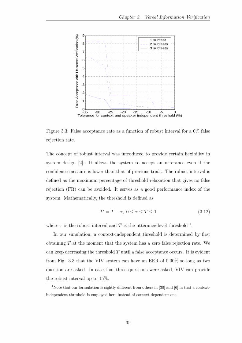
Chapter 3. Verbal Information Verification
-35 -30 -25 -20 -15 -10 -5 00
1
2
3
4
5
6
7
8
9
Tolerance for context and speaker independent threshold (%)
Fal
se A
ccep
tanc
e w
ith U
tter
ance
Ver
ifica
tion
(%)
1 subtest2 subtests3 subtests
Figure 3.3: False acceptance rate as a function of robust interval for a 0% false
rejection rate.
The concept of robust interval was introduced to provide certain flexibility in
system design [2]. It allows the system to accept an utterance even if the
confidence measure is lower than that of previous trials. The robust interval is
defined as the maximum percentage of threshold relaxation that gives no false
rejection (FR) can be avoided. It serves as a good performance index of the
system. Mathematically, the threshold is defined as
T ′ = T − τ, 0 ≤ τ ≤ T ≤ 1 (3.12)
where τ is the robust interval and T is the utterance-level threshold 1.
In our simulation, a context-independent threshold is determined by first
obtaining T at the moment that the system has a zero false rejection rate. We
can keep decreasing the threshold T until a false acceptance occurs. It is evident
from Fig. 3.3 that the VIV system can have an EER of 0.00% so long as two
question are asked. In case that three questions were asked, VIV can provide
the robust interval up to 15%.
1Note that our formulation is sightly different from others in [30] and [6] in that a context-
independent threshold is employed here instead of context-dependent one.
35

Chapter 3. Verbal Information Verification
3.4 Application and Further Improvement
Constructing databases is a must for almost all speech applications. Recorded
voices need to be compared against the prompted texts. This is an essential step
to make the data useful. However, manual verification and annotation is very
time consuming and expensive in terms of efforts, simply because the amount of
speech database is usually large. VIV’s capability of verifying subwords make
it a natural choice for the task of database validation. It can pinpoint those
erroneous recordings from tens of thousands utterances. This is indeed very
useful in practice.
Refining of the VIV system can be done in the following ways. First, speaker-
independent (SI) models can be replaced by speaker-dependent (SD) models in
utterance segmentation in that the SD models tend to produce more consistent
phoneme segmentation than the SI models. Second, speaker-dependent and
context-dependent threshold can be used instead of the speaker-independent
and context-independent threshold.
3.5 Summary
In this chapter, verbal information verification for speaker authentication is
introduced. The main approach to VIV, utterance verification and its key com-
ponents are described in detail. In particular, we have justified our choice of
the confidence measure through experimental study. Practical considerations
for security issues has been suggested. Sequential utterance verification hereby
has been employed in achieving higher level of security. Finally, a practical
application have been suggested.
36

Chapter 4
Model Design for Cantonese
Verbal Information Verification
4.1 General Considerations
In the VIV process as described in the previous chapter, the target models are
used to provide time alignment of the subword segments, and to produce the
likelihood log P (On|λn) for each subword. The accuracy of time alignment de-
pends on the acoustic models used. Context-dependent (CD) acoustic modeling
at phoneme level is considered to be most appropriate for target modeling. On
the other hand, anti-models should be designed to separate the data (speech
containing the expected subwords) from the non-data (speech not containing
the expected subwords) as far as possible [31].
4.2 The Cantonese Dialect
As one of the major Chinese dialects, Cantonese is the mother tongue of 60
million population in Southern China and Hong Kong. Cantonese is a mono-
syllabic and tonal language. Each Chinese character is pronounced as a single
syllable carrying a specific tone. Each syllable can be divided into an Initial and
a Final. The Initial is typically a consonant while the Final consists of a vowel
nucleus and an optional nasal or stop coda [32][33]. Throughout our research,
37

Chapter 4. Model Design for Cantonese Verbal Information Verification
the phonemic transcription scheme proposed by the Linguistic Society of Hong
Kong (LSHK) is adopted [34].
4.3 Target Model Design
Cantonese has 20 Initials and 53 Finals, constituting about 660 base syllables
[32]. In continuous speech recognition of Cantonese, CD Initial-Final (IF) mod-
els, namely BiIF or TriIF models 1, have been commonly used [32]. Decision-tree
tying method was commonly adopted to tackle the problem of sparse training
data [35]. In our research, the target models are Speaker-independent (SI) Bi-
IFs as they can produce reasonable recognition accuracy at affordable model
complexity and computation cost [36]. Each Initial model is a HMM with 3
states and each Final model has 5 states. These HMMs were trained on a con-
tinuous speech database, named CUCALL, which was collected over telephone
at the Chinese University of Hong Kong [23]. For base syllable recognition,
these acoustic models attained an accuracy of 54.61% in large-vocabulary con-
tinuous speech recognition (LVCSR). Fig. 4.1 shows the typical result of forced
alignment done by both manual and automatic approach. Compared to the
manual alignment, the resulted automatic time alignment are fairly acceptable
for subword based utterance verification though the model may not be good
enough for general speech recognition applications.
4.4 Anti-Model Design
4.4.1 Role of Normalization Techniques
The most significant factor affecting speaker authentication performance is the
variation of the signal characteristics from trial to trial (inter-session variability
and variability over time) [37]. Variations arise from the speakers themselves,
from differences in recording and transmission conditions, and from background
1BiIF refers to the right context dependent IF model and TriIF refers to the left and right
context dependent IF model
38

Chapter 4. Model Design for Cantonese Verbal Information Verification
Figure 4.1: Illustration of manual alignment compared with state-of-the-art au-
tomatic alignment on the utterance “baat-saam-gau-jat-ng-baat-sei-jat-jat-jat”,
each panel shows, from top to bottom: (a) the waveform, (b) the spectrogram,
(c) time axis (d) the manual alignment, and (e) the automatic alignment
noise. It is impossible for people to repeat an utterance precisely in the same
way from trial to trial. It is well known that samples recorded in one session
are much more correlated than those recorded in separate sessions. There are
also long-term changes in voices, e.g., aging.
It is important for speaker authentication systems to accommodate to
these variations. There are mainly two types of normalization techniques
that have been tried; one in the parameter domain, and the other in the dis-
tance/similarity domain.
A typical normalization technique of parameter domain is the Cepstral Mean
Substraction (CMS) [13], which has been proved to be very effective for speech
and speaker recognition applications.
As one of the normalization methods for distance (similarity, likelihood)
domain, likelihood ratio test is effective to improve the performance of both
SV and VIV system. The likelihood score tends to be more stable and less
variable than the unnormalized reference model score [3]. The question here
is how to construct anti-models that would provide the normalizing or anti-
likelihood score. There have been many individual suggestions [7][31]. However,
the general principles for anti-model design have not been seriously investigated.
39

Chapter 4. Model Design for Cantonese Verbal Information Verification
4.4.2 Context-dependent versus Context-independent
Anti-models
To facilitate the hypothesis test in Cantonese VIV (See Section 2, Chapter
3), anti-models for different Initials and Finals need to be established. The
anti-models can be either context-dependent (CD) or context-independent (CI)
[31][38]. In Mandarin VIV [6], it was reported that the performance with CD
anti-models is worse than that by CI anti-models.
Let a be the subword unit being modeled and XaY be one of its contextual
variation, where X and Y denote the left and right context respectively. In CD
anti-modeling, the anti-model for XaY is trained by the data that are labeled
as XaY , where a 6= a. In other words, a training token for the anti-model must
have different subword identity, i.e. a 6= a but the same context, i.e. X and
Y . Those segments in which both subword identity and context are different
from XaY are excluded from training. If an impostor utterance contains such
an “unseen” segment, the anti-model would generate a relatively low likelihood
and a false acceptance (FA) error may occur. On the other hand, CI anti-models
do not have the problem because all tokens with different subword identity, no
matter what contexts they have, are used for training. CI anti-models are easily
constructed, and usually have more training data than CD models. This makes
the parameter estimation more reliable. In this study, we propose the use of CI
anti-models.
4.4.3 General Approach to CI Anti-modeling
For each Initial/Final model, a corresponding anti-model needs to be trained
for the verification task. Then there would be 20 Initial anti-models and 53
Final anti-models. The phonological structure of Chinese language implies that
an Initial must be followed by a Final. For each Initial model, all training data
for other Initials should be used to train its anti-model, and those for Finals
are not used. The same training strategy applies also to the anti-modeling of
Finals. This kind of anti-models is referred to as Global anti-models.
40

Chapter 4. Model Design for Cantonese Verbal Information Verification
4.4.4 Sub-syllable Clustering
However, for training an Initial/Final Global anti-model, data from all other
phonemes are used. This may render the resulted multivariate pdf very smooth
and thus lack of discriminative power. To deal with this deficiency, the CI
sub-syllable models are grouped based on their confusability [8]. The Initial
and Final models are treated separately. As a result, six and nine clusters are
generated for Initials and Finals respectively. The clustering of sub-syllable
can be based on the confusion matrix resulted from LVCSR experiments or the
K-means clustering algorithm that minimizes the overall inter-syllable group
distance [38]. Clustering results based on these two approaches are shown in
Table 4.1 and Table 4.2 respectively.
Models ID (#) Sub-syllable Cohort Set
Initials 1 (3) [j],[l],[w]
2 (4) [p],[t],[k],[kw]
3 (4) [null],[m],[n],[ng]
4 (4) [g],[d],[b],[gw]
5 (3) [c],[z],[s]
6 (2) [f],[h]
Finals 1 (9) [aa],[aau],[aat],[aap],[aan],[aam],[aak],[aai],[aang]
2 (8) [an],[at],[ap],[an],[am],[ak],[ai],[ang]
3 (7) [o],[ou],[ot],[on],[ok],[oi],[ong]
4 (8) [i],[ik],[im],[in],[ip],[it],[iu],[ing]
5 (6) [u],[ui],[uk],[un],[ut],[ung]
6 (4) [e],[ei],[ek],[eng]
7 (6) [eot],[eon],[eoi],[oeng],[oe],[oek]
8 (3) [yu],[yun],[yut]
9 (2) [ng],[m]
Table 4.1: Cantonese Sub-syllable Clustering based on Confusion Matrix
The two methods produce somewhat similar results. In this thesis, we chose
41

Chapter 4. Model Design for Cantonese Verbal Information Verification
Models ID (#) Sub-syllable Cohort Set
Initials 1 (2) [j],[l]
2 (4) [p],[t],[k],[kw]
3 (4) [null],[m],[n],[ng]
4 (3) [g],[d],[b]
5 (4) [c],[z],[s],[f]
6 (2) [gw],[w]
Finals 1 (9) [aa],[aau],[aat],[aap],[aan],[aam],[aak],[aai],[aang]
2 (8) [an],[at],[ap],[an],[am],[ak],[ai],[ang]
3 (7) [o],[ou],[ot],[on],[ok],[oi],[ong]
4 (8) [i],[ik],[im],[in],[ip],[it],[iu],[ing]
5 (6) [u],[ui],[uk],[un],[ut],[ung]
6 (4) [e],[ei],[ek],[eng]
7 (6) [eot],[eon],[eoi],[oeng],[oe],[oek]
8 (3) [yu],[yun],[yut]
9 (2) [ng],[m]
Table 4.2: Cantonese Sub-syllable Clustering based on K-means Clustering
to construct anti-models based on confusion matrix approach.
4.4.5 Cohort and World Anti-models
Given a sub-syllable unit (Initial or Final), speech data labeled as any other
units within the same cluster are used to train the anti-model of this unit. In
this way, the anti-model becomes a characterization of the most confusable or
competitive sub-syllable units. This is similar to the Cohort background models
in speaker verification. Therefore, they are referred to as Cohort anti-models.
There is another kind of anti-models which is known as World anti-models
[18][7]. In this case, all units in the same cluster share an anti-model, which
is trained by the data from all the other clusters. For performance comparison
among different anti-modeling methods, we define the following terms:
42

Chapter 4. Model Design for Cantonese Verbal Information Verification
• In-set impostoring: A impostor utterance happens to contain a subword
that is confusable with the correct one, i.e., the impostor and true ones
are in the same cohort set.
• Out-set impostoring: A impostor utterance happens to contain a subword
that is not confusable with the correct one, i.e., the impostoring and true
ones are in different cohort sets.
Theoretically, the Cohort anti-models could reject those in-set impostoring
subwords quite well. Meanwhile, it may wrongly admit those out-set impos-
toring ones. On the other hand, the World anti-models would reject those
out-set impostoring subwords properly while accepting those in-set impostoring
ones mistakenly. It is therefore natural to combine the decisions from the two
methods to achieve the optimal performance since they are complementary to
each other. This method is referred to as combined Cohort-and-World (C&W)
anti-models. The joint decision is made based on score-level fusion, i.e.
S = α · Sworld + (1− α) · Scohort (4.1)
where S is the combined subword-level confidence score, Sworld and Scohort are
the confidence scores produced by World and Cohort methods respectively. In
Eq. (4.1), α is a weighting factor ranging from 0 to 1.
From the implementation point of view, there are usually sufficient training
data for the World anti-models, but not for the Cohort anti-models. In addition,
the time needed for the training of different anti-models varies as shown in Table
4.3.
Anti-model Cohort World Global
Time Consumption 24 hours 72 hours 14*24 hours
Table 4.3: Comparisons of training time of different anti-models (Training were
carried out on a PC with Pentium 4 processor)
43
Chapter 4. Model Design for Cantonese Verbal Information Verification
4.4.6 GMM-based Anti-models
Parametric models have became the predominant approach to pattern classifi-
cation problems. The advantage is that the models can be defined with a small
number of parameters, e.g., means and covariance matricies. Once those param-
eters are estimated from training samples, the whole distribution is completely
specified. Two issues need to be considered beforehand. The first is about the
model structure and the second is about the complexity of models ever selected.
Intuitively, the model structure or topology of anti-models should be the
same as that of the target models. In other words, the anti-models for Initial
and Final would be left-to-right HMMs that have 3 and 5 states respectively. In
[8], we proposed to use GMM-based anti-models instead of HMM-based ones.
And the result highly favors the proposed method. GMM-based anti-models
consistently outperformed HMM-based anti-models. Explanations to this phe-
nomenon are given below.
HMM is well-known for its capability to characterize the spectral properties
of dynamic speech signals [39]. The HMM models not only the underlying
speech sounds, but also the temporal sequencing among these sounds. When
modeling the phonetic units using an HMM, we assume that all the observation
sequences labeled as the same phonetic unit do hold the same or similar temporal
sequence, which is an important property to be captured by the HMM. We can
say that temporal structure modeling is advantageous for target model.
But it is not the case for anti-modeling. As we stated before, the anti-model
for a phonetic unit is trained by the speech data from many other phonetic units.
Among the training data from a specific phoneme, there does exist a character-
istic inherent temporal sequence. However, among training data from distinct
phonemes, this inter-phoneme temporal relation does not exist and the funda-
mental assumption of HMM acoustic modeling becomes inappropriate. Tempo-
ral structure of speech should not be taken into account in the anti-modeling
for VIV. This is similar to speaker modeling in text-independent speaker recog-
nition, where Gaussian components can be considered to be modeling the broad
class of phonetic sounds.
44

Chapter 4. Model Design for Cantonese Verbal Information Verification
Gaussian Mixture Models could be thought of as a single-state HMM with
a Gaussian mixture observation density, or an ergodic Gaussian observation
HMM with fixed equal transition probabilities. It can also be viewed as a hybrid
between parametric and nonparametric density model. Like a parametric model,
it has the structure and parameters that control the behavior of the density in
a known way, but without the constraints that the data must be of a specific
distribution type. Like a nonparametric model, the GMM has many degrees of
freedom to allow arbitrary density modeling, without undue computation and
storage demands [18].
Therefore, by using GMM for anti-modeling, the temporal sequence beneath
the observation vectors from different phonemes is implicitly blurred or not
taken into account. We believe that this structure is more appropriate.
4.5 Simulation Results and Discussions
Experiments are carried out for each of the anti-model design described in the
previous section.
The acoustic features used in VIV experiments are the first 12 mel-frequency
cepstral coefficients (MFCC) together with the short-time energy. The features
are energy normalized and cepstral mean normalized. By including the first and
second order derivatives of the parameters, each feature vector has 39 compo-
nents.
4.5.1 Speech Databases
The speech database used to train speaker-independent BiIF target models and
context-independent anti-models is also part of CUCALLTM. The corpus con-
sisting of continuous Cantonese sentences is selected. Table 4.4 summarizes the
statistics on this corpus.
The testing database used for VIV performance evaluation is the same as
the one used in SV experiment (See Section 4, Chapter 2).
45

Chapter 4. Model Design for Cantonese Verbal Information Verification
Training Set Testing Set
# of Speakers 679 80
# of Utterances 17.6K 2.4K
# of Syllables 237.6K 23.3K
Total Length 29.6 (hours) 2.5 (hours)
Avg SenLen 13.5 9.7
(# of Syllables)
Table 4.4: Statistics of the Sentence Corpus of CUCALL
4.5.2 Effect of Model Complexity
The number of mixture components per state for each anti-model affects the
overall system performance. The optimal number of mixtures are determined
empirically (See Fig. 4.2, which is based on Global anti-models).
Effects of Model Complexity
0.00%
1.00%
2.00%
3.00%
2 4 8 16 32
Number of mixture components
Equal
Err
or
Rat
e
GMM-based Anti-
models
HMM-based Anti-
models
Figure 4.2: Equal Error Rate vs. Model Complexity
From these results, we conclude that the optimal number of mixture com-
ponents of each state is 2 for HMM-based anti-models, and 16 for GMM-based
anti-models. These optimal number of mixture components are selected in the
following experiments.
46

Chapter 4. Model Design for Cantonese Verbal Information Verification
4.5.3 Comparisons among different Anti-models
First, we compare among the anti-models that are constructed differently. We
need to determine the optimal weighting factor α in the combined Cohort-and-
World (C&W) anti-models. As shown in Fig. 4.3, the optimal value of α
0
0.5
1
1.5
2
2.5
3
0 0.1 0.2 0.3 0.4 0.5 0.6 0.7 0.8 0.9 1
Weighting factor alpha
Equal
Err
or
Rat
e (%
)
HMM-based Anti-
models
GMM-based Anti-
models
Figure 4.3: Equal Error Rate vs. Weighting factor α in combined Cohort-and-
World (C&W) anti-models
is found to be 0.9 for both HMM-based and GMM-based anti-models. This
indicates that more confidence is put on the World anti-models.
Fig.4.4 shows the Detection Error Tradeoff (DET) curves for the anti-models.
Both the World and the Global anti-models outperform the Cohort anti-models
significantly. It is out of our expectation to note that Global anti-models can
achieve fairly low EER. Among all anti-models, the combined C&W GMM-
based anti-models yields the lowest EER of 0.45%. This indeed reveals that
they take advantages of both methods. The worst EER of 2.8% is produced
by the Cohort HMM-based anti-models. It is observed that the performance
of all GMM-based anti-models are consistently better than that of HMM-based
ones. This agrees with our findings in [8], though the experimental data are
different. Apart from the superior verification performance, GMM-based anti-
models have the advantage of maintaining simplicity in training and decoding
phases.
It is worth emphasizing that all the above experimental results were ob-
tained using the same subword time alignments and the acoustic models used
47

Chapter 4. Model Design for Cantonese Verbal Information Verification
0.1 0.2 0.5 1 2 5 10 20 40
0.1
0.2
0.5
1
2
5
10
20
40
False Alarm probability (in %)
Mis
s p
roba
bilit
y (in
%)
Speaker Detection Performance
C&W+GMMWorld+GMMGlobal+GMMCohort+GMMWorld+HMMC&W+HMMGlobal+HMMCohort+HMM
Figure 4.4: Comparisons of system performance based on various context-
independent anti-models.
for alignment have a base syllable recognition accuracy of less than 60%. This
clearly indicates that the design of anti-models is most critical in VIV, where
the time alignment doesn’t have to be very precise.
4.5.4 Discussions
There are several factors causing decision errors. These include acoustic envi-
ronment and handset mismatches between the training and testing conditions.
In our experiments, digit strings are used as test utterances. It is highly likely
that the impostor utterance contains similar phoneme sequences to the client
one. The proposed method of anti-modeling can maximize the capability of
VIV to make the correct decisions. It is expected that error-free performance
could be achieved when VIV is integrated into SV.
48

Chapter 4. Model Design for Cantonese Verbal Information Verification
4.6 Summary
Based on the UV framework, there are three key modules that determine the
system performance. They are the target models, anti-models and confidence
measures respectively. Among them, the design of anti-models play the most
important role since they greatly affect the overall performance of VIV system.
In this chapter, we have studied different design strategies for anti-modeling
for Cantonese verbal information verification. A thorough discussion of various
methods of constructing anti-models has been provided. An new technique in
anti-modeling was proposed and the motivations were presented.
From the experimental results on VIV, it can be concluded that the com-
bined Cohort-and-World GMM-based anti-models perform the best among all
designs of anti-models. It is also found that the recognition accuracy of the
target models did not much affect the system performance. We believe that
our findings can be applicable to other languages, especially those with similar
phonological structure with Cantonese, e.g., Mandarin.
49

Chapter 5
Integration of SV and VIV
In the previous chapters, we have described SV and VIV systems individually. In
this chapter, we explore how to integrate the two systems to make a more reliable
decision. The approaches to information fusion have been used in different
applications of pattern classification like speech recognition and handwriting
recognition. This problem remains to be an open topic and thorough discussions
would not be the goal of this study. In this chapter, we formulate the integration
problem into a binary classification problem with 2D input features. Three ways
of integration are suggested and investigated. Fundamentals of these methods
are briefly presented and their strength and weakness are also addressed.
5.1 Introduction
SV and VIV are using different information carried in the utterances. We
expected that combining the expertise of these individual systems will further
improve the verification performance.
Fig. 5.1 and Fig. 5.2 show the histogram plots of SV and VIV scores,
respectively. Obviously, there is always some overlaps between the client and the
impostor data for both systems. In other words, it is impossible to completely
separate these data no matter what threshold is used. If the likelihood scores
from two verification systems are combined, it is possible to find a hyperplane or
curve to completely separate the client and impostor data, as shown in Fig. 5.3.
50

Chapter 5. Integration of SV and VIV
-0.4 -0.2 0 0.2 0.4 0.6 0.8 1 1.2 1.40
50
100
150
200
250
300
SV scores
Co
unts
Client dataImpostor data
Figure 5.1: Histogram for the SV likelihood scores for two classes. One class is
from client data and the other one is from impostor data. No single threshold
value will serve to unambiguously discriminate between the two classes.
0.1 0.2 0.3 0.4 0.5 0.6 0.7 0.8 0.9 10
50
100
150
200
VIV scores
Cou
nts
Client dataImpostor data
Figure 5.2: Histogram for the VIV likelihood scores for two classes. One class is
from client data and the other one is from impostor data. No single threshold
value will serve to unambiguously discriminate between the two classes.
51

Chapter 5. Integration of SV and VIV
This motivates us to seek for appropriate methods to integrate the two systems.
-0.4 -0.2 0 0.2 0.4 0.6 0.8 1 1.2 1.40.1
0.2
0.3
0.4
0.5
0.6
0.7
0.8
0.9
1
SV scores
VIV
sco
res
Client dataImpostor data
Figure 5.3: Scatter plot of VIV scores vs SV scores. The dark line could serve
as a decision boundary of our classifier.
In speaker authentication, system integration can be done at different levels
such as feature-level and model-level. In our case, the same kind of features
is used in both systems. We will focus our discussion on combining likelihood
scores of both systems.
The integrated authentication system consists of three components: SV sys-
tem, VIV system and a pattern classifier or the decision maker. A block diagram
is depicted as in Fig. 5.4. The input to the pattern classifier is a two-dimensional
vector that is composed of the output of two systems. There have been differ-
ent ways proposed to integrate SV and VIV. In [40], a speech recognizer is
used to analyze the user’s answer to a specific question. With these results,
the system can restrict the hypothesized space of candidates. Then a speaker
recognizer handles the users’ access for this smaller candidates set. Researchers
at Bell Lab proposed to combine the two verification systems incrementally [1].
In their work, VIV is used in the first 4-5 accesses. Speaker’s utterances are
recorded and used to train the speaker model for SV. Later on, the authenti-
52

Chapter 5. Integration of SV and VIV
Speech
SV system
VIV system
Pattern
Classifier
Accept
Reject
Ssv(X)
Sviv(X)
Speaker
models
Speech
lexicons
Figure 5.4: Structure of the integrated authentication system
cation process can be switched from VIV to SV. In [41], an intuitive method
called voting was presented to integrate two systems with two shared thresh-
olds, and compared the performance with using speaker-specific thresholds for
two independent system. A novel framework based on non-standard Support
Vector Machines (SVMs) technique was proposed in [42]. This method makes it
possible to adjust the tradeoff between false acceptance error and false rejection
error without loss of good generalization performance of conventional SVMs.
In the following sections, we will investigate the methods of voting, support
vector machines, and gaussian-based classifiers respectively.
5.2 Voting Method
The basic idea of voting is simple and intuitive. It is to compare the SV likeli-
hood and the VIV likelihood with their respective thresholds and the decision
rule is that both likelihoods or either one has to be greater than the threshold
for a user access to be accepted. The method can be represented as:
Vvoting(X, I,K) =
+1, if Ssv(X) > θsv and/or Sviv(X) > θviv
−1, otherwise(5.1)
In this section, we address the problems of how to set up the thresholds in
both the SV and VIV systems and how to combine them to improve overall
53
Chapter 5. Integration of SV and VIV
performance.
5.2.1 Permissive Test vs. Restrictive Test
There are two different criteria of verification in the dual tests:
• Permissive Test : Speaker accepted if one of the likelihoods exceeds its
corresponding threshold
• Restrictive Test: Speaker accepted only if both likelihoods exceed the
correspondent thresholds.
In real-world applications, a system should work somewhere in between the
two extreme cases. Our solution was to use a continuous function that varies
between the two extreme cases with a controlled parameters β. Suppose that
Ls and Lv are the SV and VIV likelihoods respectively. We first normalize them
with their respective thresholds Ts and Tv as,
Lx =Lx − Tx
|Tx| , x = {s, v} (5.2)
A sigmoid function was applied for smoothing:
Sx =1
1 + e−aeLx(5.3)
The scores Ss and Sv take values between 0 and 1. Making use of these scores
the restrictive and permissive tests are implemented.
Operm = Sig2(Ss + Sv − 0.5)− 0.5
Orest = Sig2(2 · Ss · Sv − 0.5)− 0.5(5.4)
Sig2(x) =1
1 + e−bx(5.5)
Operm is −0.5 when Ls < Ts and Lv < Tv and 0.5 if one of the likelihoods exceeds
the threshold. Orest is −0.5 or 0.5 if one of likelihoods is less than the threshold
or if both likelihoods are greater than their respective thresholds. Finally, the
verification test is performed as:
V = β ·Orest + (1− β) ·Operm
V > 0 ⇒ Accepted(5.6)
54

Chapter 5. Integration of SV and VIV
5.2.2 Shared vs. Speaker-specific Thresholds
Shared Thresholds
The first possibility is to use two thresholds shared by all speakers: one for
the speaker verification likelihoods and another for the utterance verification
likelihoods.
Speaker-specific Thresholds
In case that speaker-dependent thresholds are used, two thresholds per speaker
(one per likelihood) can be computed using the development data. For each
speaker, the variation of the false acceptance rate (FAR) and false rejection rate
(FRR) against the threshold calculated for both SV and VIV systems. When
the FAR and FRR curves cross each other, the threshold leading to equal error
rate was taken. If the curves don’t cross, the used criterion was to take the
mean of the thresholds where the rates go to zero. Examples can be seen in
Fig.5.5 and Fig.5.6. In this way, we obtain two thresholds per speaker and two
-0.5 0 0.5 1 1.5 20
0.1
0.2
0.3
0.4
0.5
0.6
0.7
0.8
0.9
1
SV scores
FA
an
d F
R R
ates
FA and FR curves cross
FAFR
Threshold
Figure 5.5: Example of the criteria for taking the values of the thresholds when
FA and FR curves cross
likelihoods to perform a dual verification test.
55

Chapter 5. Integration of SV and VIV
-0.5 0 0.5 1 1.5 20
0.1
0.2
0.3
0.4
0.5
0.6
0.7
0.8
0.9
1
SV scores
FA
an
d F
R R
ates
FA and FR Curves don't cross
FRFA
Threshold
Figure 5.6: Example of the criteria for taking the values of the thresholds when
FA and FR curves do not cross
5.3 Support Vector Machines
Speaker authentication can be viewed as a binary classification problem for
which support vector machine is a natural choice of solution. Support vector
machines (SVMs) [43] have become popular due to their attractive features
and good generalization capability. They have been applied to many areas, in
particular biometrics such as speaker verification [44].
The integration of SV and VIV is a simple application of SVMs. We will
focus our discussion on the simplest cases, i.e., linear SVMs trained on linearly
separable cases. SVMs in principle can be generalized to non-linearly separable
cases.
We start with the simplest case: linear machines trained on separable data.
First, label the training data as {xi, yi}, i = 1, ..., l, yi ∈ {−1, +1}, xi ∈ Rd.
Suppose we have a hyperplane which separates the positive from the negative
examples (a “separating hyperplane”). The points x which lie on the hyper-
plane satisfy w · x + b = 0, where w is normal to the hyperplane, |b|/‖w‖ is
the perpendicular distance from the hyperplane to the origin, and ‖w‖ is the
Euclidean norm of w. Let d+(d−) denote the shortest distance from the sepa-
56

Chapter 5. Integration of SV and VIV
rating hyperplane to the closest positive (negative) example. d+d− is defined
as the “margin” of the separating hyperplane. For the linearly separable case,
the support vector algorithm simply looks for the separating hyperplane with
the largest margin. This can be formulated as follows [45]. Suppose that all
training data satisfy the following constraints:
xi ·w + b ≥ +1 for yi = +1 (5.7)
xi ·w + b ≤ +1 for yi = −1 (5.8)
They can be combined into one set of inequalities:
yi(xi ·w + b)− 1 ≥ 0 ∀i (5.9)
Consider the points for which the equality in Eq. (5.7) holds. These points lie
on the hyperplane H1 : xi ·w+ b = 1 with the normal w and the perpendicular
distance from the origin |1−b|/‖w‖. Similarly, the points for which the equality
in Eq. (5.8) holds lie on the hyperplane H2 : xi ·w + b = −1, with the normal
again w, and the perpendicular distance from the origin | − 1− b|/‖w‖. Hence
d+ = d− = 1/‖w‖ and the margin is simply 2/‖w‖. Note that H1 and H2 are
parallel and that no data points fall between them. Thus we can find the pair
of hyperplanes which gives the maximum margin by minimizing ‖w‖2, subject
to constraints of Eq. (5.9).
The solution to a typical two-dimensional case has the form shown as in Fig.
5.7. The data points for which the equality in Eq. (5.9) holds (i.e. those which
wind up lying on one of the hyperplanes H1, H2), and whose removal would
change the solution, are called support vectors. They are indicated in Fig. 5.7
by the extra circles.
Therefore, the primal problem of optimization is formulated as follows [45]:
min ‖w‖2
s.t yi · (xi ·w + b)− 1 ≥ 0, ∀i(5.10)
Normally, we will not directly solve the primal problem. We solve the dual
problem instead. The procedures in formulating dual problem are described
below [45]:
57

Chapter 5. Integration of SV and VIV
Figure 5.7: Linear separating hyperplanes for the separable case. The support
vectors are circled. (after Burges [45])
We switch to a Lagrangian formulation of the primal problem. There are
two reasons of doing this. First, the constraints of Eq. (5.9) will be replaced by
constraints on the Lagrangian multipliers themselves, which will be much easier
to handle. Second, in the formulation, the training data will only appear in the
form of dot products between vectors. This is a crucial property that allows us
to generalize the procedures to the nonlinear cases.
We introduce the positive Lagrangian multipliers αi i = 1, ..., l, one for each
of the inequality constraints in the Eq. (5.9). This gives Lagrangian:
LP(w, b, α) ≡ 1
2‖w‖2 −
l∑i=1
αi · yi(xi ·w + b) +l∑
i=1
αi (5.11)
Then, construct the dual function L∗(α), which is given below:
L∗(α) = minw,b
LP(w, b, α). (5.12)
We minimize LP with respect to w, b. Equivalently, it requires that the
gradient of LP with respect to w and b vanish, which gives the conditions:
w =∑
i
αiyixi (5.13)
∑i
αiyi = 0. (5.14)
Since these are equality constraints in the dual formulation, we can substi-
tute them into Eq. (5.10) to give the final formulation [45]
max LD =∑
i
αi − 1
2
∑i,j
αiαjyiyjxi · xj
s.t αi ≥ 0, ∀i.(5.15)
58

Chapter 5. Integration of SV and VIV
The training of support vectors (for linearly separable case) therefore is done
by maximizing LD with respect to αi, subject to constraints in Eq. (5.15) and
positivity of α, with the solution given by Eq. (5.13).
Training of SVMs are not illustrated here. It involves solving a quadratic
programming problem that scales quadratically with the number of examples.
Practical training of SVMs can use the decomposed training algorithm in [46],
where for selecting the working set, the approximation proposed by Joachims
in [47] is used.
Once the values of αi have been found from Eq. (5.12), Eq. (5.13) can then
be used to determine w. Once w is found, it can be in turn be plugged into Eq.
(5.16) to determine the value of threshold b:
b = 1− xk ·w, where yk = 1 and xk ∈ S. (5.16)
where S is a set containing the indexes to the support vectors. Ultimately, the
decision boundary can be derived as follows [48]:
f(x) = w · x + b =N∑
i=1
yiαi(x · xi) + b = 0. (5.17)
5.4 Gaussian-based Classifier
SVM is a nonparametric approach. In this section, we will investigate a para-
metric approach that could be used in our case. For parametric approaches, we
need to consider the model structure and its complexity.
In our case, the input feature is two-dimensional vector composed of SV and
VIV likelihood scores. It is therefore easy to visualize the distribution in order
to determine the appropriate structure for modeling the distribution. We use a
set of development data to visualize the data distribution as in Fig. 5.3. From
a cluster perspective, most biometric data cannot be adequately modeled by a
single-cluster Gaussian model. However, they often can be accurately modeled
via a Gaussian Mixture Model (GMM), i.e., data distribution can be expressed
as a mixture of multiple normal distributions. From Fig. 5.3, GMM seems to
be an appropriate choice in our case.
59

Chapter 5. Integration of SV and VIV
In supervised learning, several prominent estimation methods (e.g., K-means
or EM algorithms) can be used to estimate the density parameters of a GMM
statistic model. In addition, the clustering task also involves the determination
of an optimal number of clusters for GMM.
Since the two verification scores are not correlated, it is reasonable to use
the diagonal covariance matrix. Error-free performance is achieved when only
one mixture GMM is used.
After estimating the model parameters based on the development data, it is
possible to draw a decision boundary to separate the two classes and to apply
in test.
5.5 Simulation Results and Discussions
In this section, experimental results on the integration of SV and VIV will be
presented. UBM adaptation is used for the training of speaker models for SV.
The combined Cohort-and-World GMM-based anti-models are used for VIV.
The three methods of score combination are compared in terms of efficiency
and error rate. Their strength and weakness are discussed.
5.5.1 Voting Method
The development data described as in Section 4, Chapter 2 are used to derive
thresholds. As mentioned before, there are two extreme criteria to accept the
claimed identity: permissive test and restrictive test. In real-world applications,
we prefer that a system work somewhere in-between these two extremes. Thus,
two parameters that control the slope of the sigmoid function need to be deter-
mined. Based on our empirical study, they are set to be 5 and 2 respectively.
Shared Thresholds
In this experiment, the same thresholds are used for all speakers. There are
two thresholds: one for the SV likelihoods and another for the VIV likelihoods.
These shared thresholds are determined from the development data. The vari-
60

Chapter 5. Integration of SV and VIV
ation of false acceptance and false rejection rates with β (Defined in Eq. (5.6))
is shown as in Fig. 5.8. The operation point would be placed somewhere in the
area depending on the specific requirement of applications.
0 0.1 0.2 0.3 0.4 0.5 0.6 0.7 0.8 0.9 10
0.005
0.01
0.015
0.02
0.025
0.03
0.035
Alpha
Equ
al E
rro
r Rat
e
Voting method with shared thresholds
FRRFAR
EER = 0.338%
Figure 5.8: False acceptance and false rejection rates obtained using the voting
method with shared thresholds. β varies between 0 and 1
In Table 5.1, results obtained with the shared thresholds are presented. It
can be observed that, in the best case (labelled Voting 1), the improvement
compared to VIV in the FA and the FR rates are 0.25% and 0.33%, respectively.
Verification β FA Rate FR Rate
SV N/A 2.11% 0.67%
VIV N/A 0.59% 0.67%
Voting 1 0.66 0.338% 0.338%
Voting 2 0.85 0.03% 0.75%
Voting 3 0.55 0.90% 0.38%
Table 5.1: Results using voting method with shared thresholds
Speaker-specific Thresholds
In case that speaker-specific thresholds are used, there are two thresholds per
speaker and two likelihoods to perform the dual test. The experiments con-
61

Chapter 5. Integration of SV and VIV
ducted are similar to those for shared thresholds. The results are given as in
Fig. 5.9.
0 0.1 0.2 0.3 0.4 0.5 0.6 0.7 0.8 0.9 10
0.01
0.02
0.03
0.04
0.05
0.06
Beta
Equ
al E
rror
Rat
e
Voting method with Individual Thresholds
FRRFAR
EER = 0.33%
Figure 5.9: False acceptance and false rejection rates using the voting method
with individual thresholds. β varies between 0 and 1
In Table 5.2, the results obtained with speaker-specific thresholds are given.
It can be seen that, in the best case (labelled Voting 1), the improvement com-
pared to VIV in the FA and the FR rates are are 0.067% and 1.0%, respectively.
Verification β FA Rate FR Rate
SV N/A 0.46% 2.0%
VIV N/A 0.263% 1.33%
Voting 1 0.4 0.33% 0.33%
Voting 2 0.5 0.1% 0.6%
Voting 3 0.3 0.6% 0.3%
Table 5.2: Results obtained with the combined system on individual thresholds
On the whole, the voting method based on individual thresholds outperform
that using shared thresholds. It does conform to our expectation. The voting
method itself is simple and intuitive. Moreover, it allows the system to be flex-
ibly configurable as we can trade the false rejection error with false acceptance
error by simply adjusting the parameter β.
62
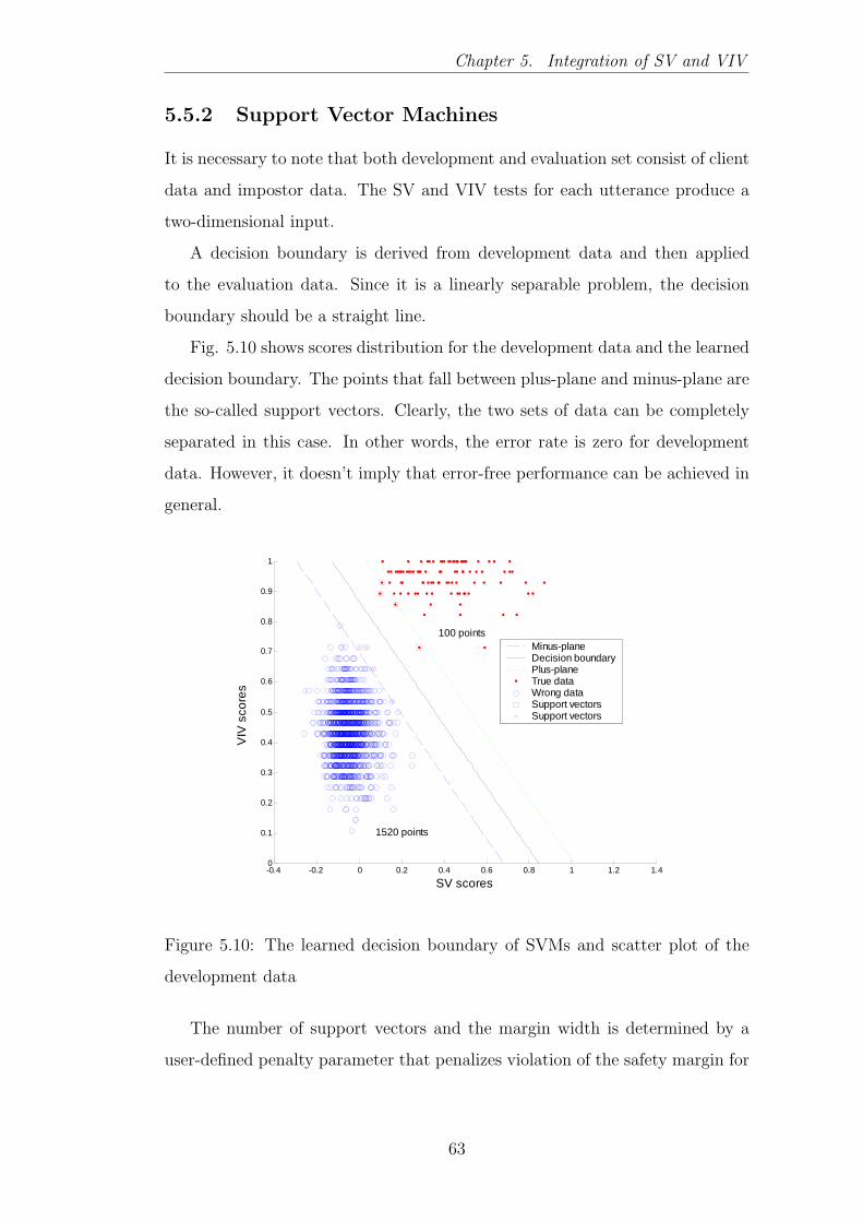
Chapter 5. Integration of SV and VIV
5.5.2 Support Vector Machines
It is necessary to note that both development and evaluation set consist of client
data and impostor data. The SV and VIV tests for each utterance produce a
two-dimensional input.
A decision boundary is derived from development data and then applied
to the evaluation data. Since it is a linearly separable problem, the decision
boundary should be a straight line.
Fig. 5.10 shows scores distribution for the development data and the learned
decision boundary. The points that fall between plus-plane and minus-plane are
the so-called support vectors. Clearly, the two sets of data can be completely
separated in this case. In other words, the error rate is zero for development
data. However, it doesn’t imply that error-free performance can be achieved in
general.
-0.4 -0.2 0 0.2 0.4 0.6 0.8 1 1.2 1.40
0.1
0.2
0.3
0.4
0.5
0.6
0.7
0.8
0.9
1
SV scores
VIV
sco
res
Minus-planeDecision boundaryPlus-planeTrue dataWrong dataSupport vectorsSupport vectors
100 points
1520 points
Figure 5.10: The learned decision boundary of SVMs and scatter plot of the
development data
The number of support vectors and the margin width is determined by a
user-defined penalty parameter that penalizes violation of the safety margin for
63

Chapter 5. Integration of SV and VIV
all development data. Generally, the larger the penalty parameter, the more
narrow the margin width.
-0.4 -0.2 0 0.2 0.4 0.6 0.8 1 1.2 1.40
0.1
0.2
0.3
0.4
0.5
0.6
0.7
0.8
0.9
1
SV scores
VIV
sco
res
Client dataImpostor dataMinus-planeDecision boundaryPlus-plane
1520 points
300 points
Figure 5.11: The learned decision boundary and scatter plot of the evaluation
data
The learned decision boundary is applied to the evaluation data and the
result is shown as in Fig. 5.11. It is observed that only one client data point la-
beled is misclassified. The false rejection error is 0.33% and the false acceptance
error is 0%.
This result might serve as a true reflection of power of SVMs, especially for
the linearly separable cases. However, since the decision boundary is learned
from the development data, it will inevitably result in a rigid ratio between
FAR and FRR. In other words, it is difficult to adjust the tradeoff between false
acceptance error and false rejection error.
5.5.3 Gaussian-based Classifier
In this section, we present the experimental results of using the Gaussian clas-
sifier. The procedures are to learn a decision boundary from the development
64

Chapter 5. Integration of SV and VIV
data and then apply it to the evaluation. It is almost the same as SVM ap-
proach except that the decision boundary might be a curve instead of a straight
line.
First, we need to train the GMMs for client and impostor classes using
the EM algorithm based on the development data. In general, the numbers of
centers and different covariance types (“diag” or “full”) affect the performance.
From experimental results, it was found that one center for each class plus
diagonal covariance matrix can provide error-free performance. However, this
may not be a generalizable performance. If there are much more training data
involved, we can use more centers and the full covariance matrix to represent
the data distribution.
-0.5 0 0.5 10
0.1
0.2
0.3
0.4
0.5
0.6
0.7
0.8
0.9
1
SV scores
VIV
sco
res
1.5
1.5
1.5
1.5
Client DataTrained CentresImpostor Data
100 points
1520 points
Figure 5.12: The learned decision boundary of GMM-based classifier and scatter
plot of the development data
Fig. 5.12 shows the score distribution of development data and the learned
decision boundary. Along the decision boundary, the probability of belonging
to the client data equals to the probability of belonging to the impostor data.
We can use this decision boundary to classify new data points. Experimental
results are illustrated in Fig. 5.13. The classification rate is 100% and this
65
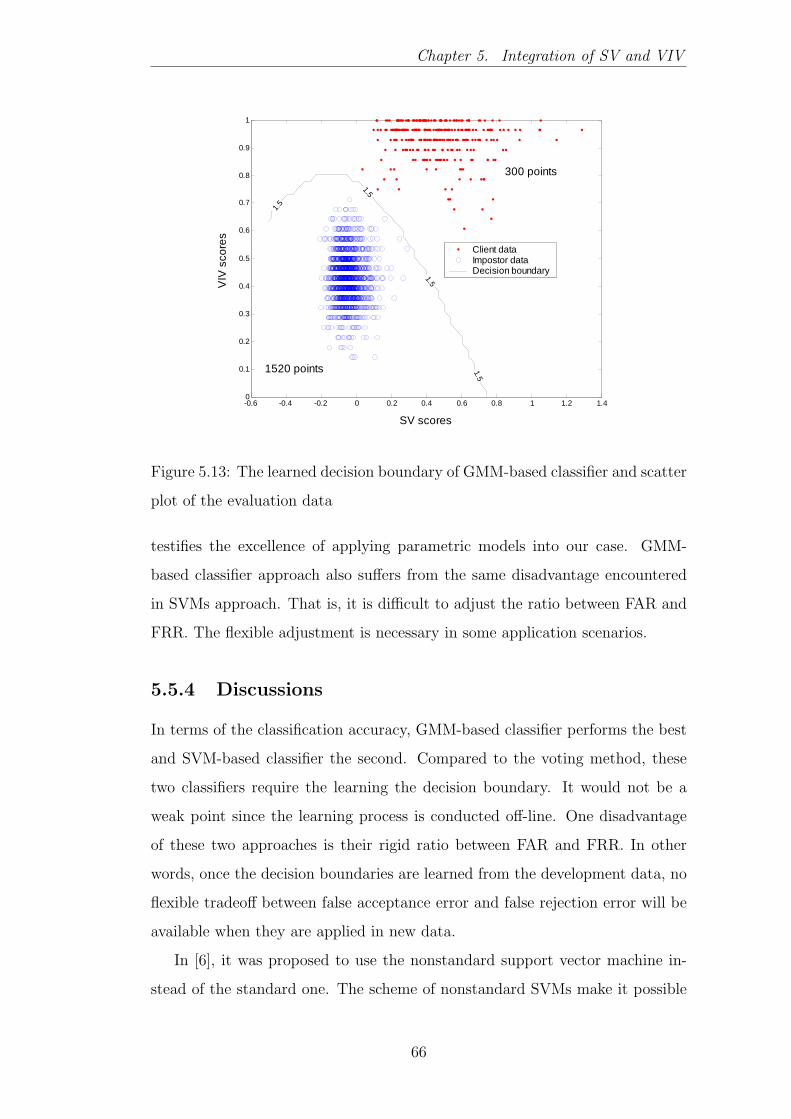
Chapter 5. Integration of SV and VIV
-0.6 -0.4 -0.2 0 0.2 0.4 0.6 0.8 1 1.2 1.40
0.1
0.2
0.3
0.4
0.5
0.6
0.7
0.8
0.9
1
SV scores
VIV
sco
res
1.5
1.5
1.5
1.5
Client dataImpostor dataDecision boundary
1520 points
300 points
Figure 5.13: The learned decision boundary of GMM-based classifier and scatter
plot of the evaluation data
testifies the excellence of applying parametric models into our case. GMM-
based classifier approach also suffers from the same disadvantage encountered
in SVMs approach. That is, it is difficult to adjust the ratio between FAR and
FRR. The flexible adjustment is necessary in some application scenarios.
5.5.4 Discussions
In terms of the classification accuracy, GMM-based classifier performs the best
and SVM-based classifier the second. Compared to the voting method, these
two classifiers require the learning the decision boundary. It would not be a
weak point since the learning process is conducted off-line. One disadvantage
of these two approaches is their rigid ratio between FAR and FRR. In other
words, once the decision boundaries are learned from the development data, no
flexible tradeoff between false acceptance error and false rejection error will be
available when they are applied in new data.
In [6], it was proposed to use the nonstandard support vector machine in-
stead of the standard one. The scheme of nonstandard SVMs make it possible
66

Chapter 5. Integration of SV and VIV
to adjust the tradeoff between false acceptance error and false rejection error
without loss of the generalization performance of traditional SVMs.
The voting method has the advantage of being more configurable. That is,
the operating point of the system is easily controlled by a parameter α instead
of having to adjust the whole set of thresholds. This makes it appealing to
many applications.
5.6 Summary
In this chapter, three approaches to the integration of two verification systems
have been studied and their fundamentals have been given. In particular, for-
mulation and derivation of support vector machines for the simplest case have
been provided in detail.
Experimental results on three methods have been presented. It turns out all
of them are quite effective. Strength and weakness of these three methods have
also been discussed. It has to be emphasized here that what we suggested for
combining two verifiers is not a through treatment of combining classifiers but
could serve as the milestone for the further research.
67

Chapter 6
Conclusions and Suggested
Future Works
6.1 Conclusions
Biometric authentication systems are becoming indispensable for protecting life
and property. Researches on biometric authentication are receiving great at-
tention. With the recent technological advances, automatic authentication has
become a practical reality. Among various biometrics, voice is one of the most
natural and the least obtrusive biometric measures [49].
In this thesis, we have studied speaker authentication techniques for Can-
tonese, though the techniques are not language-specific by its nature. Identity-
related information conveyed in a spoken utterance mainly encompasses voice
characteristics and verbal content. Speaker verification (SV) and verbal infor-
mation verification (VIV) are two techniques used to authenticate these infor-
mation individually. A SV system has been developed using state-of-the-art
techniques. A novel technique of modeling alternative hypotheses has been pro-
posed for VIV. We have also sought to integrate SV and VIV to exploit their
complementary.
Speaker variability affects the performance of an authentication system sig-
nificantly. The likelihood scores computed for a true speaker varies from one
trial to another, even if the same content is spoken. This makes it difficult to
68

Chapter 6. Conclusions and Suggested Future Works
set an optimal threshold to differentiate the clients from the impostors. Nor-
malization techniques are applied to deal with the errors caused by such vari-
ability. Likelihood ratio test (LRT) is one of the most powerful methods for
binary-decision problems. It has been successfully applied to both SV and VIV
decisions. Within the framework of LRT, we need to build a model to represent
alternative hypotheses.
In speaker verification, building such a model is referred to as background
speaker modeling. Although there is no theoretical solution to this problem,
many practically effective methods have been devised. Universal background
modeling (UBM) is becoming the pre-dominant approach. In this case, all
speakers share an all-in-one background model, i.e. the UBM, which is typically
a Gaussian mixture model. The expectation-maximization (EM) algorithm is
commonly used to estimate model parameters. All speaker models are adapted
from this UBM. Experiments on 20 Cantonese speakers have been conducted to
compare this method with the conventional Cohort method. The results showed
that the UBM adaptation outperforms the Cohort modeling significantly. The
best performance with an equal error rate (EER) of 1.5% is achieved using the
UBM adaptation approach along with front-end endpoint detection.
In verbal information verification, modeling alternative hypotheses is known
as anti-modeling. There are many considerations in the process of constructing
anti-models, such as the way of pooling subword units, the model structure and
the model complexity. Each of these issues has been addressed individually in
the previous research. However, we don’t see a thorough discussion in litera-
ture on the design of anti-models. In this study, GMM-based anti-models are
proposed to replace the conventional HMM-based ones. GMM does not impose
any temporal constraint among the sound classes. Experiments have demon-
strated the superior performance of the proposed method. Besides, GMM is
computationally more efficient than HMM in both training and testing phase.
This research has confirmed that GMM-base anti-modeling for VIV is a simple
yet effective method.
Experimental results showed that the combined Cohort-and-World GMM-
69

Chapter 6. Conclusions and Suggested Future Works
based anti-models perform the best among all designs. The best performance
achieved has an EER of 0.6%. It is found that the recognition accuracy of the
target models did not much affect the VIV performance. We believe that our
findings would be applicable to other languages, especially those with similar
phonological structure, e.g. Mandarin.
Finally, for the integration of SV and VIV system, three methods have been
evaluated. This is formulated as the problem of classifying two-dimensional
patterns into two classes. Experimental results have demonstrated the effec-
tiveness of these methods. In particular, by using the Gaussian-based classifier,
error-free performance can be achieved. This indicates the overall excellence of
the proposed Cantonese speaker authentication system.
6.2 Summary of Findings and Contributions of
This Thesis
The major contributions from this research are summarized below:
• It is the first study in VIV for Cantonese dialect.
• Detailed discussions on anti-modeling for VIV have been provided, i.e.
pooling training data for anti-models, model structure and model com-
plexity.
• GMM as a better representation of VIV anti-models than the generic
HMM. Its superiority has been testified by experimental study.
• Different ways of integrating SV and VIV at system level have been inves-
tigated. These include the intuitive Voting method, the popular Support
Vector Machines and the generative Gaussian Classifier. Experimental
results reflect the effectiveness of the integrated system. Error-free per-
formance is achieved.
• The proposed method is not language specific and can be extended to
other languages, such as Mandarin and English. Also, the anti-model
70

Chapter 6. Conclusions and Suggested Future Works
design for VIV can be directly applied in the general tasks of utterance
verification.
• The VIV techniques have been used to verify the CUSV speech database.
It turns out to be very convenient for postprocessing collected speech data
since it releases great human effort from tedious validation work.
• A real-time Cantonese VIV demo system has been built using the proposed
method.
6.3 Future Perspective
6.3.1 Integration of Keyword Spotting into VIV
A versatile VIV system should be able to handle flexible input styles rather
than the rigid keyword sequences. This desirable feature will make the dialog
more user-friendly and more intelligent. Keyword spotting technique can serve
as a natural solution for this task. In general, ASR techniques can be applied in
the front-end to generate a N best list of admissible candidates and utterance
verification techniques can be used to do re-scoring and select the best one to
be compared against the prescribed threshold.
6.3.2 Integration of Prosodic Information
Current speaker authentication techniques rely almost exclusively on low-level
acoustic features extracted from speech signals. These features convey informa-
tion about the physical traits of the speaker’s vocal apparatus. They are known
to have a relatively high sensitivity to noise and channel mismatch. Humans use
several levels of perceptual cues for speaker authentication. Examples of high-
level information are speaking rate, pitch patterns, idiosyncratic word/phrase
usage, laughter, etc [50]. These high-level features often represent learned traits
of a speaker related to the speaker’s social status, personality, educational back-
ground, etc. Furthermore, they are assumed to be much more robust to noise
71

and channel distortion. Nowadays, researcher have paid more and more atten-
tion on the extraction and utilization of these high-level perceptual cues, and
explore the ways of making them contributing to original system. The Super-
SID project at the 2002 JHU CLSP Summer Workshop was initiated for this
purpose (See [50]).
Cantonese is well known for its tonal characteristics. Prosodic informa-
tion plays an important role in large-vocabulary Cantonese speech recognition
(LVCSR). Prosodic information are encoded in duration, intensity and pitch
contour. Phonetic and prosodic information can be integrated and used for
Cantonese speaker authentication.
For text-independent SV, phonetic and prosodic can be integrated at several
levels. For VIV, prosodic information can be utilized to assist verification deci-
sion. Some pioneering works have been reported in [51]. It is generally believed
that by properly fusing high- and low-level features, the performance of speaker
authentication will be greatly improved.
72

Appendix A
A Cantonese VIV
Demonstration System
In order to illustrate effectiveness and high performance of VIV technique, we
build a real-time Cantonese VIV demo system. This demo system is run on
the Windows platform and developed on CURec, the new speech recognition
engine. Let’s show this demo through an example.
First, we have built a database for storing the users’ profiles. Each user
is asked to provide 18 pieces of personal information such as “What is your
telephone number?”. Each of them is assigned an user id from 000 to 050.
During the testing phase, the major interface of this demo system is shown
as in Fig. A.1. When an user tries to log in the system, he/she will claim
his/her identity by presenting the user id and click “Login”. There are also
other buttons on the main interface which are used for automatic registration
and for control by system administrator.
After that, a question will be randomly selected from the question pool that
is constructed based on the 18 pieces of pre-recorded personal information (Fig.
A.2). There is a confidence bar that is used to indicate how many questions
the claimed user has correctly responded. Originally, the bar is fully charged.
After clicking the “Start Recording” button, the user’s response will be recorded
and passed through the VIV system. A utterance-level confidence score will be
generated for this answer. In order to make the system more practical, we set
73

Figure A.1: Main interface of VIV system
two thresholds for the utterance-level confidence score. One is at about 0.72 and
another is at about 0.55. If the utterance-level confidence score is lower than
0.55, this answer will be rejected immediately and the system will proceed to ask
next randomly selected question. If the second question is not satisfied again,
the claimed user will be rejected by the system. If the utterance-level confidence
score is higher than 0.55 and lower than 0.72, the user will be given a second
chance to answer the same question. If it is higher than 0.72, the answer will be
accepted immediately. The user has to answer at least 2 questions correctly to
pass the system. Correspondingly, when an answer is rejected, the confidence
bar will drop by 30%. When it drops to 0, the user will be rejected. When the
user answers one question rightly, the bar will remain unchange or increase by
30%.
Figure A.2: Sample question
Fig. A.3 shows the results in detail about the verification process. The
74
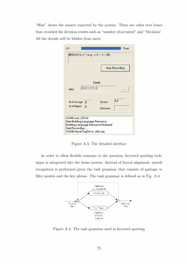
“Hint” shows the answer expected by the system. There are other text boxes
that recorded the decision results such as “number of accepted” and “Decision”.
All the details will be hidden from users.
Figure A.3: The detailed interface
In order to allow flexible response to the question, keyword spotting tech-
nique is integrated into the demo system. Instead of forced alignment, speech
recognition is performed given the task grammar that consists of garbage or
filler models and the key phrase. The task grammar is defined as in Fig. A.4
Key PhraseFiller ModelCantonese garbage modelCantonese subword sequence
UtteranceStart UtteranceEndFigure A.4: The task grammar used in keyword spotting
75

By using this grammar, users may respond to the system more freely. For
example, the answer could be “I graduated from the Chinese University of Hong
Kong” instead of the rigid “the Chinese University of Hong Kong”. We have
tested on the new system and results are satisfactory.
Target models used in this demo system are fixed as right context-dependent
Initial-Final models and anti-models are the proposed GMM-based ones.
76

Bibliography
[1] Q. Li, B.-H. Juang, Q. Zhou, and C.-H. Lee, “Automatic verbal information
verification for user authentication,” IEEE Trans. Acoustics, Speech, Signal
Processing, vol. Vol.8, No.5, Sept. 2000.
[2] Q. Li, B.-H. Juang, Q. Zhou, and C.-H. Lee, “Verbal information verifica-
tion,” in Proc. Eurospeech, pp. 839–842, Sept. 1997.
[3] A. Rosenberg and S. Parthasarathy, “Speaker background models for con-
nected digit password speaker verification,” in Proc. IEEE Int. Conf. on
Acoustics, Speech, Signal Processing, (Atlanta, GA).
[4] S. Parthasarathy and A. Rosenberg, “General phase speaker verification
using sub-word background models and likelihood-ratio scoring,” in Proc.
Int. Conf. on Speech Language Processing, (Philadelphia, PA).
[5] D. Reynolds, “Comparison of a background normalization methods for
text-independent speaker verification,” in Proc. Eurospeech, pp. 963 – 966,
Sept. 1997.
[6] X. Li and K. Chen, “Mandarin verbal information verification,” in
Proc. IEEE Int. Conf. on Acoustics, Speech, Signal Processing, (Orlando,
Florida), May 2002.
[7] Y. Liu and B. Xu, “Comparison of anti-model training algorithms in man-
darin verbal information verification,” in NCMMSC6, (Shenzheng, China),
Nov. 2001.
77

[8] C. Qin and T. Lee, “Cantonese verbal information verification using GMM-
based anti-models,” in Proc. Int. Symposium on Chinese Spoken Language
Processing, (Hong Kong), Dec. 2004.
[9] F. Bimbot, J.-F. Bonastre, C. Fredouille, G. Gravier, I. Margin-
Chagnolleau, S. Meignier, T. Merlin, J. Ortega-Garcia, D. Petrovska-
Delacretaz, and D. A. Reynolds, “A tutorial on text-independent speaker
verification,” EURASIP Journal on Applied Signal Processing, pp. 430–
451, 2004.
[10] A. Oppenheim and R. W.Schafer, Discrete-Time Signal Processing. Engle-
wood Cliffs, NJ: Prentice Hall, 1989.
[11] A. Oppenheim and R. Schafer, “Homomorphic analysis of speech,” IEEE
Transactions on Audio and Electroacoustics, vol. 16, No. 2, pp. 221–226,
June 1968.
[12] F. Soong and A. Rosenberg, “On the use of instantaneous and transi-
tional spectral informationin speaker recognition,” IEEE Trans. Acoustics,
Speech, Signal Processing, vol. 36, Issue:6, pp. 871 – 879, June 1988.
[13] S. Furui, “Cepstral analysis technique for automatic speaker verification,”
IEEE Trans. Acoustics, Speech, Signal Processing, vol. ASSP-29, pp. 254
– 272, Apr. 1981.
[14] D. Reynolds, “An overview of automatic speaker recognition technology,”
in Proc. IEEE Int. Conf. on Acoustics, Speech, Signal Processing, (Orlando,
Florida), May 2002.
[15] F. Soong, A. Rosenberg, L. Rabiner, and B. Juang, “A vector quantization
approach to speaker recognition,” in Proc. IEEE Int. Conf. on Acoustics,
Speech, Signal Processing, pp. 387 – 390, Apr. 1985.
[16] A. Poritz, “Linear predictive hidden markov models and the speech signal,”
in Proc. IEEE Int. Conf. on Acoustics, Speech, Signal Processing, pp. 1291
– 1294, May 1982.
78

[17] D. A. Reynolds, “Speaker identification and verification using gaussian
mixture models,” Speech Communication 17, pp. 91–108, 1995.
[18] D. A. Reynolds, T. F. Quatieri, and R. B. Dunn, “Speaker verification using
adapted gaussian mixture models,” Digital Signal Processing 10, pp. 19–41,
2000.
[19] A. Higgins, L. Bahler, and J. Porter, “Speaker verification using random-
ized phrase prompting,” Digital Signal Processing, vol. 1, No. 2, pp. 89 –
106, 1991.
[20] A. Rosenberg, J. Delong, C.-H. Lee, B.-H. Juang, and F. Soong, “The use
of cohort normalized scores for speaker verification,” in Proc. Int. Conf. on
Speech Language Processing, (Banff, Canada), pp. 599–602, Nov. 1992.
[21] A. Martin, G. Doddington, T. Kamm, M. Ordowski, and M. Przybocki,
“The det curve in assessment of detection task performance,” in Proc.
Eurospeech, pp. 1895–1898, Sept. 1997.
[22] G. R. Doddington, M. A. Przybocki, A. F. Martin, and D. A. Reynolds,
“The nist speaker recognition evaluation - overview, methodology, systems,
results, perspective,” Speech Communication 31, pp. 225–254, 2000.
[23] T. Lee, W. Lo, and P. Ching, “Towards highly usable and robust spoken
language technologies for chinese,” in Proceedings of the Second China-
Japan Natural Language Processing Joint Research Promoting Conference,
(Beijing, China), Nov. 2002.
[24] Q. Li and B.-H. Juang, “Speaker verification using verbal information veri-
fication for automatic enrollment,” in Proc. IEEE Int. Conf. on Acoustics,
Speech, Signal Processing, (Seattle, WA).
[25] M. Rahim, C.-H. Lee, and B.-H. Juang, “Robust utterance verification
for connected digits recognition,” in Proc. IEEE Int. Conf. on Acoustics,
Speech, Signal Processing, (Detroit, MI), pp. 285–288, May 1995.
79

[26] M. Rahim, C.-H. Lee, B.-H. Juang, and W. Chou, “Discriminative utter-
ance verification using minimum string verification error (msve) training,”
in Proc. IEEE Int. Conf. on Acoustics, Speech, Signal Processing, (Atlanta,
GA).
[27] T. Kawahara, C.-H. Lee, and B.-H. Juang, “Combining key-phrase detec-
tion and subword-based verification for flexible speech understanding,” in
Proc. IEEE Int. Conf. on Acoustics, Speech, Signal Processing, (Munich,
Germany), pp. 1159–1162, Apr. 1997.
[28] E. Lleida and R. Rose, “Efficient decoding and training procedures for
utterance verification,” in Proc. IEEE Int. Conf. on Acoustics, Speech,
Signal Processing, (Atlanta, GA).
[29] R. Sukkar, A. Setlur, M. Rahim, and C.-H. Lee, “Utterance verification
of keyword string using word-based minimum verification,” in Proc. IEEE
Int. Conf. on Acoustics, Speech, Signal Processing, (Atlanta, GA).
[30] Q. Li, S. Parthasarathy, and A. E. Rosenberg, “A fast algorithm for stochas-
tic matching with application to robust speaker verification,” in Proc. IEEE
Int. Conf. on Acoustics, Speech, Signal Processing, (Munich, Germany),
pp. 1543–1547, Apr. 1997.
[31] P. Ramesh, C.-H. Lee, and B.-H. Juang, “Context dependent anti subword
modeling for utterance verification,” in Proc. Int. Conf. on Speech Language
Processing, (Sydney, Australia), Nov. 1998.
[32] T. Lee, W. Lo, P. Ching, and H. Meng, “Spoken language resource for can-
tonese speech processing,” Speech Communication 36, pp. 327–342, 2002.
[33] W. Lo, “Cantonese phonology and phonetics: an engineering introduction,”
tech. rep., Speech Processing Group, Digital Signal Processing Labortory,
Department of Electronic Engineering, the Chinese University of Hong
Kong, 2000.
80

[34] O. kan Yue-Hashimoto, Studies in Yue Dialects 1: Phonology of Cantonese.
Cambridge University Press, 1972.
[35] W. Reichl and W. Chou, “Decision tree state tying based on segmental
clustering for acoustic modeling,” in Proc. IEEE Int. Conf. on Acoustics,
Speech, Signal Processing, (Seattle, WA).
[36] Y. W. Wong, “Large vocubulary continuous speech recognition for can-
tonese,” MPhil thesis, The Chinese University of Hong Kong, Department
of Electronic Engineering, Aug. 2000.
[37] R. A. Cole, J. Mariani, H. Uszkoreit, A. Zaenen, and V. Zue, Fundamentals
of Speech Recognition. Center for Spoken Language Understanding: Oregon
Graduate Institute, 1995.
[38] Y.-J. Chen, C.-H. Wu, and G.-L. Yan, “Utterance verification using
prosodic information for mandarin telephone speech keyword spotting,” in
Proc. IEEE Int. Conf. on Acoustics, Speech, Signal Processing, (Phoenix,
Arizona).
[39] L. Rabiner and B.-H. Juang, Fundamentals of Speech Recognition. Engle-
wood Cliffs, NJ: Prentice Hall, 1993.
[40] S. H. Maes, “Conversational biometrics,” in Proc. Eurospeech, (Budapest,
Hungary), Sept. 1999.
[41] L. Rodriguez-Linares and C. Garcia-Mateo, “A novel technique for the com-
bination of utterance and speaker verification system in a text-dependent
speaker verification task,” in Proc. Int. Conf. on Speech Language Process-
ing, (Sydney, Australia), Nov. 1998.
[42] Y. Liu, P. Ding, and B. Xu, “Using nonstandard svm for combination of
speaker verification and verbal information verification in speaker authen-
tication system,” in Proc. IEEE Int. Conf. on Acoustics, Speech, Signal
Processing, (Orlando, Florida), May 2002.
81

[43] V. Vapnik, Statistical Learning Theory. Wiley, 1998.
[44] V. Wan, Speaker Verification Using Support Vector Machine. Ph.D thesis,
University of Sheffield, June 2003.
[45] C. J. Burges, “A tutorial on support vector machines for pattern recog-
nition,” Data Mining and Knowledge Discovery, vol. 2(2), pp. 121–167,
1990.
[46] E. Osuna, R. Freund, and F. Girosi, “An improved training algorithm for
support vector machines,” in Proc. of IEEE NNSP’97, (Amelia Island, FL),
pp. 24–26, Sept. 1997.
[47] T. Joachims, “Making large-scale svm learn practical,” in Advanced in
Kernel Methods - Support Vector Learning (B. Scholkopf, B. Burges, and
A. S. (Eds), eds.), pp. 121–167, Cambridge, Massachusetts: The MIT Press,
1999.
[48] S. Kung, M. Mak, and S. Lin, Biometric Authentication, A Machine Learn-
ing Approach. Prentice Hall Information and System Sciences Series, 2004.
[49] Y. Y. Tam, “Subband spectral features for speaker recognition,” MPhil
thesis, The Chinese University of Hong Kong, Department of Electronic
Engineering, 2004.
[50] J. P. Campbell, D. A. Reynolds, and R. B. Dunn, “Fusing high- and
low-level features for speaker recognition,” in Proc. Eurospeech, (Geneva,
Switzerland), Sept. 2003.
[51] C.-H. Wu, Y.-J. Chen, and G.-L. Yan, “Use of prosodic information for
mandarin word verification,” Proc. Natl. Sci. Counc. ROC(A), vol. Vol.23,
No.4, pp. 488–494, 1999.
82