velocity response curves support the role of continuous
TRANSCRIPT

Velocity Response Curves Support the Role of Continuous Entrainment in
Circadian Clocks
Stephanie R. Taylor∗, Alexis B. Webb†, Linda R. Petzold‡, and Francis J. Doyle III§¶
∗Department of Computer Science, Colby College
Waterville, ME 04901
†Department of Biology, Washington University
Saint Louis, MO 63130
‡Department of Computer Science, University of California Santa Barbara
Santa Barbara, CA 93106
§Department of Chemical Engineering, University of California Santa Barbara
Santa Barbara, CA 93106
¶Corresponding Author: Email: [email protected]. Phone: 805-893-8133. Fax: 805-893-4731
Running Title: Velocity Response Curves

Abstract
Circadian clocks drive endogenous oscillcations in organisms across the tree of life. The Earth’s daily
light/dark cycle entrains these clocks to the environment.Two major theories of light entrainment have
been presented in the literature – the discrete theory and the continuous theory. Here, we re-introduce the
concept of a velocity response curve (VRC), which describeshow a clock’s speed is adjusted by light.
We examine entrainment of a mathematical model of the circadian clock using both the VRC and phase
response curves (PRCs) for long (circa 12 h) pulses of light.Our results demonstrate that the VRC and
PRCs together predict clock behavior under full photoperiod entrainment, supporting the contention that
the clock is being adjusted continuously. Further, we show that much of the insights gained from PRCs
and the discrete theory of entrainment can be used to understand continuous entrainment. For example,
we show that the presence of a deadzone in the VRC explains whyphotoskeleton and full photoperiod
entrainment yield the same phase of entrainment.
Keywords: phase response curves, mathematical modeling, circadianclock, sensitivity analysis, entrain-
ment, velocity response curves
1

Introduction
In organisms across the tree of life, circadian clocks coordinate daily behaviors with the environment by
responding to external cues, or zeitgebers. Left in constant conditions, these clocks will oscillate, but with
a period that is not exactly 24 hours. Entrainment allows zeitgebers, such as daily light/dark cycles, tem-
perature cycles, and social interactions to adjust the period and synchronize the clock with the environment.
Historically, the circadian field has employed two theoriesof light entrainment – the discrete theory of Colin
Pittendrigh and the continuous theory of Jurgen Aschoff1. The discrete theory assumes that the light/dark
transitions at dawn and dusk reset or phase shift the clock instantly, correcting its mismatch with the envi-
ronment. These transitions are mimicked experimentally asshort pulses of light. Thus, the phase response
curve (PRC), which measures the phase shift resulting from ashort pulse of light, is the main experimental
tool and has been a good predictor of entrainment behaviors (Daan and Pittendrigh, 1976a). Alternatively,
the continuous theory assumes that light acts on the clock throughout the circadian cycle. It is supported
by evidence that the period of an animal’s clock depends uponthe levels of light in constant conditions
(Aschoff, 1979). It is now generally accepted that both theories are at least partially valid. Reconciling them
remains a perplexing but important question.
Three unified theories of entrainment have been presented. First, Pittendrigh himself (Daan and Pit-
tendrigh, 1976b) considered the possibility of velocity response curves (VRCs) (Swade, 1969), which are
similar in shape to PRCs but describe changes to the clock’s phasevelocity. In this case, the majority of
the phase shifting would take place at dawn and dusk not because the light/dark transition is important but
because the clock’s velocity cannot be altered during the middle of the day (see Figure 1A). Second, the
“limit cycle” interpretation of Peterson (1980) raises thepossibility that there are two separate limit cycles
used by the molecular clock – one in constant darkness (DD) and another in constant light (LL). Movement
between the two cycles would cause discrete and continuous entrainment to look similar at the behavioral
level but would be different at the molecular level (Johnsonet al., 2003). Third, Beersmaet al. (1999)
present a phase-only model incorporating continuous effects (using a period response curve) and discrete
effects (using a phase response curve), which are treated asindependent from one another. This model takes
into account variability in light patterns, illustrating that a combination of the two effects yields the most
robust entrainment behavior. All three theories were developed prior to the development of mathematical
1For recent perspectives on entrainment, see (Johnson et al., 2003) and (Roenneberg et al., 2003) and the references containedwithin.
2

modeling at the molecular level. Thus they have not been evaluated at the molecular level – a necessity for
determining the biological mechanisms for entrainment.
In mammals, the master clock resides in the suprachiasmaticnuclei (SCN) of the hypothalamus where
transcriptional feedback networks drive oscillations in thousands of neurons. The SCN receives environ-
mental timing information through the retinohypothalamictract. The pathway of light information is not
well characterized, but there is evidence that short pulsesof light cause rapid induction of mRNA transcrip-
tion from clock genesPeriod1 (Per1) andPeriod2 (Per2) (Reppert and Weaver, 2001). Additional evidence
indicates that the effects of light are attenuated over timevia either saturation or adaptation (Comas et al.,
2006; Comas et al., 2008). Further, for nocturnal mammals, light fails to cause any phase shifts during a
clock’s internal, or subjective, day. This is evident in theso-called deadzone of their PRCs. It has been
argued that a clock-controlled, or phase-dependent, gate prevents light from entering the system during the
day (Roenneberg et al., 2003; Geier et al., 2005).
In the present work, we study the process of entrainment using a mathematical model of the mouse
circadian clock that incorporates both “saturation” and phase-dependent light gates. We use a limit cycle
model and an analytical VRC to demonstrate the relationshipbetween the PRC of the discrete theory and
the period-modulation of the continuous theory, thus providing mathematical support for a VRC unified
theory of entrainment. We demonstrate the ability of our unified theory to predict properties such as the
phase angle of entrainment and show that much of the intuition gained by studying PRCs can be used to
understand continuous effects of light. We also show that the presence of a deadzone of the VRC explains
why pulse and continuous stimuli at subjective dawn yield the same response and further that the VRC acts
as the basis on which PRCs of differing durations are formed.
3

0 6 12 18 24−2
0
2
Circadian Time
VR
C in
DD
A
0 6 12 18 24−2
0
2
Zeitgeber Time t (h)
VR
C in
LD
B
0 6 12 18 24−2
0
2
Zeitgeber Time t (h)
VR
C in
LD
C
0 6 12 18 24−0.8
−0.6
−0.4
−0.2
0
0.2
0.4
0.6
Zeitgeber Time t (h)
Pha
se D
iffer
ence
(ci
rcad
ian
h)
D
Figure 1: Velocity response curves (VRCs) in free-run and under entrainment. A) The VRC has a shapesimilar to that of a PRC, but shows changes in the clock’s velocity. When the VRC is one, then light (L = 1)doubles the speed of the clock. The VRC is shown as its changesunder B) full photoperiod (12:12) and C)skeleton photoperiod (1:10:1:12) entrainment. D) Shown isthe difference between zeitgeber time and thephase of the clock under both entrainment scenarios (solid line for the full photoperiod, dashed line for theskeleton photoperiod). Positive values indicate the internal phase is ahead of zeitgeber time. The dark graybackground indicates night in both scenarios. The light gray background from ZT1 to ZT11 indicates theperiod of darkness during photoskeleton entrainment.
Materials and Method
Phase Sensitivity Measures
Limit Cycles and Phase
A limit cycle model is a deterministic model whose solution is a stable, attracting cycle, orlimit cycle γ. It
is defined by a set of autonomous nonlinear ordinary differential equations
x(t) = f(x(t,p),p) (1)
4

wherex ∈ Rn is the vector of states andp ∈ R
m is the vector of (constant) parameters. A simulation of the
freerunning clock (i.e. with the nominal DD parameter set) will be along the limit cycle (i.e.xγ(t,p)) and
will have periodτ (i.e. xγ(t,p) = xγ(t + τ,p).
The phaseφ of a clock model is indicated byposition on limit cycle, e.g the position of the peak ofPer2
mRNA is associated with CT7 (φ = 7)2. In constant conditions,φ(xγ(t)) will progress at the same rate as
external, or zeitgeber, time3. The single ODE describing its trajectory is
dφ(xγ(t,p))
dt= 1, φ(xγ
0) = 0 (2)
wherexγ0 is the position on the limit cycleγ associated with dawn (Kuramoto, 1984; Brown et al., 2004)4.
When light acts on the clock model, it is manifested as a parametric perturbation. Parametric perturba-
tion causes the state trajectory to leave the DD limit cycle.Thus, our definition of phase must be extended
to positions off the limit cycle. For this, we use isochrons.An isochron is a hyperplane that acts as a “same-
time locus” (Winfree, 2001); over time, all points on a single isochron approach the same position on the
limit cycle, and therefore all share the same phase. In the interest of concise notation, we writeφ(x(t,p)) as
φ(x(t)) below.
Dynamic Phase Tracking
To predict the phase dynamics in response to a series of infinitesimally short perturbations, we consider
two forms of the phase evolution equation and infinitesimal phase response curve. They are rooted in
theory established by Winfree and Kuramoto, and extended byothers (Kuramoto, 1984; Kramer et al.,
1984; Winfree, 2001; Brown et al., 2004; Taylor et al., 2008). The oldest measure, the state impulse PRC
(sIPRC)5, predicts the phase response to a direct manipulation of a state trajectory. The sIPRC is a vector,
with one entry sIPRCk for each statexk:
sIPRCk(φ(xγ(t))) =∂φ∂xγ
k
(φ(xγ(t))),
2CT7 is circadian time 7, that is 7 circadian hours after subjective dawn. In keeping with standard practice, we associateCT0with internal, or subjective, dawn and CT12 with subjectivedusk.
3ZT (zeitgeber time) is used to describe the timing of an entraining agent and we associate ZT0 with the first occurrence oflights on (i.e. external dawn).
4For a more in-depth discussion ofφ defined in the presence of perturbations, see (Brown et al., 2004).5The sIPRC is called the “infinitesimal PRC” orz in much of the literature (Brown et al., 2004). In (Taylor et al., 2008) we
named it the sIPRC to differentiate it from curves associated with parametric perturbation.
5

and can be interpreted as the infinitesimal phase shift (∂φ) resulting from a direct perturbation to thekth entry
of a solution along the limit cycle. More often, the sIPRC is used to predict the change in phase velocity, as
part of a phase evolution equation:
dφ(x(t))dt
= 1+sIPRC(φ(x(t))) ·S(φ(x(t)), t) (3)
whereS is a vector of stimuli and is written as a function of either phase (i.e. the stimulus is from a clock-
controlled source) or time (i.e. the stimulus is dependent on zeitgeber time). Frequently, this model is used
to capture oscillatory behavior of electrically stimulated neurons as they fire.
In earlier work (Taylor et al., 2008), we introduced analogous formulae for tracking the phase dynamics
in the presence ofparametric perturbation. The parametric impulse PRC (pIPRC) predictsthe phase shift
(∂φ) resulting from an infinitesimally short duration, infinitesimally small in magnitude perturbation to a
parameter. The pIPRC for thejth parameter is defined
pIPRCj(φ(x(t))) =ddt
∂φ∂p j
(φ(x(t)) (4)
=∂
∂p j
dφdt
(φ(x(t))) (5)
= VRCj. (6)
From Eq. 5, it is clear that the pIPRC is also a velocity response curve – it predicts the change in phase
velocity dφ/dt due to a perturbation in parameterp j. For the remainder of the present work, we refer to
pIPRCj as VRCj or “the VRC.”
To track the effects of parametric perturbation to component j over time, we rewrote the phase evolution
equation using the VRC according to
dφ(x(t))dt
= 1+VRCj(φ(x(t)))s j(x(t), t) (7)
wheres j(x(t), t) = ∆p j(x(t), t).
6

The VRC is related to the sIPRC according to
VRCj(x(t)) =N
∑k=1
sIPRCk(x(t))∂ fk
∂p j(x(t))
= sIPRC·∂f
∂p j
whereN is the number of states.
The stimuli in the phase evolution equations are then related according to
Si(φ(x(t)), t) =∂ fi
∂p j(φ(x(t))) s j(φ(x(t)), t),
and Eqs. 3 and 7 are related by:
dφ(x(t))dt
= 1+sIPRC(φ(x(t))) ·S(φ(x(t)), t)
= 1+sIPRC(φ(x(t))) ·∂f
∂p j(φ(x(t))) s j(φ(x(t)), t)
= 1+VRCj(φ(x(t))) s j(φ(x(t)), t).
Gating Light
To accurately reproduce light response data, we must accurately model the signal as it is seen by the clock.
Experimental evidence indicates that light is gated by a “saturation” gate and a phase-dependent gate (which
creates the deadzone) (Roenneberg et al., 2003; Comas et al., 2007; Comas et al., 2008). Thus, our model
must incorporate such gates. In Figure 2 we show a conceptualpicture of the clock and the input pathway
of light. L(t) is the level of light in the environment. It passes through aninitial gateGI, which attenuates
L(t) due to saturation and adaptation. The signal leaving gateGI then passes through the phase-dependent
gateGP and finally into the core clockX , where it activates the transcription ofPer.
We model the system shown in Figure 2, using a published modelof the circadian clock as the core
oscillator. The initial gateGI mimics the response reduction and restoration dynamics observed in (Comas
et al., 2006; Comas et al., 2007). Comas et al. (2006) reported a 78% attenuation in the response to light
arriving after the first hour of a pulse. It is an open questionas to the response during the first hour6, but
6The response to short pulses of light has been studied for hamsters and mice (see, for example, (Nelson and Takahashi, 1999)),
7

Figure 2: Input Schematic. Light gates are shown as rectangles, the core clock as a circle, and input andfeedback are shown as arrows. The external light cueL passes through the initial gate, which produces anattenuated light signalGI(L). This signal then passes through the phase-dependent gate,which uses clockcomponentsXGC to compute further signal attenuation. The result isGP(GI(L),XGC), which manipulatesthe core clockX . The core clock sends output signals to peripheral oscillators which, in turn, may feed backto the clock. The output processes are shown in gray and are not included in the models under consideration.
Fig. 5 in (Comas et al., 2007) suggests there is no significantattenuation.7 We make the assumptions that
(a) there is no attenuation during the first hour, and (b) the attenuation of the phase response is directly
proportional to the attenuation in the signal. Thus, we model the initial gate such that it allows all light
through for the first hour. Thereafter, it allows exponentially less light through, asymptoting at 22%. In the
dark, the system restores its response capabilities according to an exponential curve. For the restoration, we
use the exponential curve estimated by Comas et al. (2007).
We model the initial gateGI as a function of lightL and gate variableG. G has an upper steady-state
Gss > 1 and a lower steady-state 0.22. WhenG ≥ 1, all light is allowed through. Otherwise, it is attenuated
according to
GI(t,L) = min(G(t),1)L. (8)
G is designed to travel fromGss to 1 in the first hour of a light signal. It then decreases to within 5% of its
some with results indicating that light effects saturate at15 minutes (Khammanivong and Nelson, 2000), but because these lightpulses were much more intense (4960 lux) than those in Comas et al (2006; 2007) (100 lux), we model results in Comas et al.(2006; 2007) only.
7Fig. 5 (Comas et al., 2007) shows a linear increase in the response for pulses up to 1 hour long (the first pulse of a two-pulseexperiment). A linear relationship between the pulse duration and the magnitude of the response indicates no attenuation.
8

lower steady-state 0.22 in 0.8 hours. In darkness,G recovers its magnitude until it reachesGss8. The ODE
for G is
dGdt
=
ln(0.005)(G−0.22), L = 0 (Dark)
0, L > 0andG > Gss (Light)
9.9344, L > 0andG ≤ Gthresh (Light),
(9)
whereGss = 0.78e− ln(0.005) +0.22.
Geier et al. (2005) incorporated a phase-dependent gate into a model of the mouse clock (Becker-
Weimann et al., 2004) by assuming that some (possibly not modeled) clock components are cycling in
phase with modeled components. These unknown components interact with the pathway of light within the
cell, preventing the signal from increasing the transcription of Per during the subjective day. We construct a
similar gate, using a function bounded between 0 (no increase allowed) and 1 (the signal is ungated).
Because the trace of the gate-controlling clock component(s) XGC is not known, we assume it is a linear
combination of the modeled components (i.e. the state variables in the core clock model)
XGC(x) = γN
∑i=1
αixi. (10)
The gate uses a functionY designed to allow maximal light through whenXGC is at its peak and to block
passage of light when at its trough, i.e.
Y (XGC) =
0, XGC < A
1C
(
16X3
GC − A+B4 X2
GC + AB2 XGC + A3
12 −A2B
4
)
, A ≤ XGC ≤ B
1, XGC > B.
(11)
whereC = −B3
12 + AB2
4 − A2B4 + A3
12 andA andB bound an interval between the minimum and maximum value
of theXGC oscillation, i.e. mint(XGC(t)) ≤ A < B ≤ maxt(XGC(t)). The amount of light allowed through the
phase dependent gate is then
GP(t,L,XGC) = GI(t,L) ·Y (XGC). (12)
We assume that the gated signal increases the rate ofPer transcription as an additive term, i.e. if the
8Although the recovery ofG is modeled as linear, the exponential saturation causes theeffects of light to follow the exponentialrestoration curve published in (Comas et al., 2007).
9
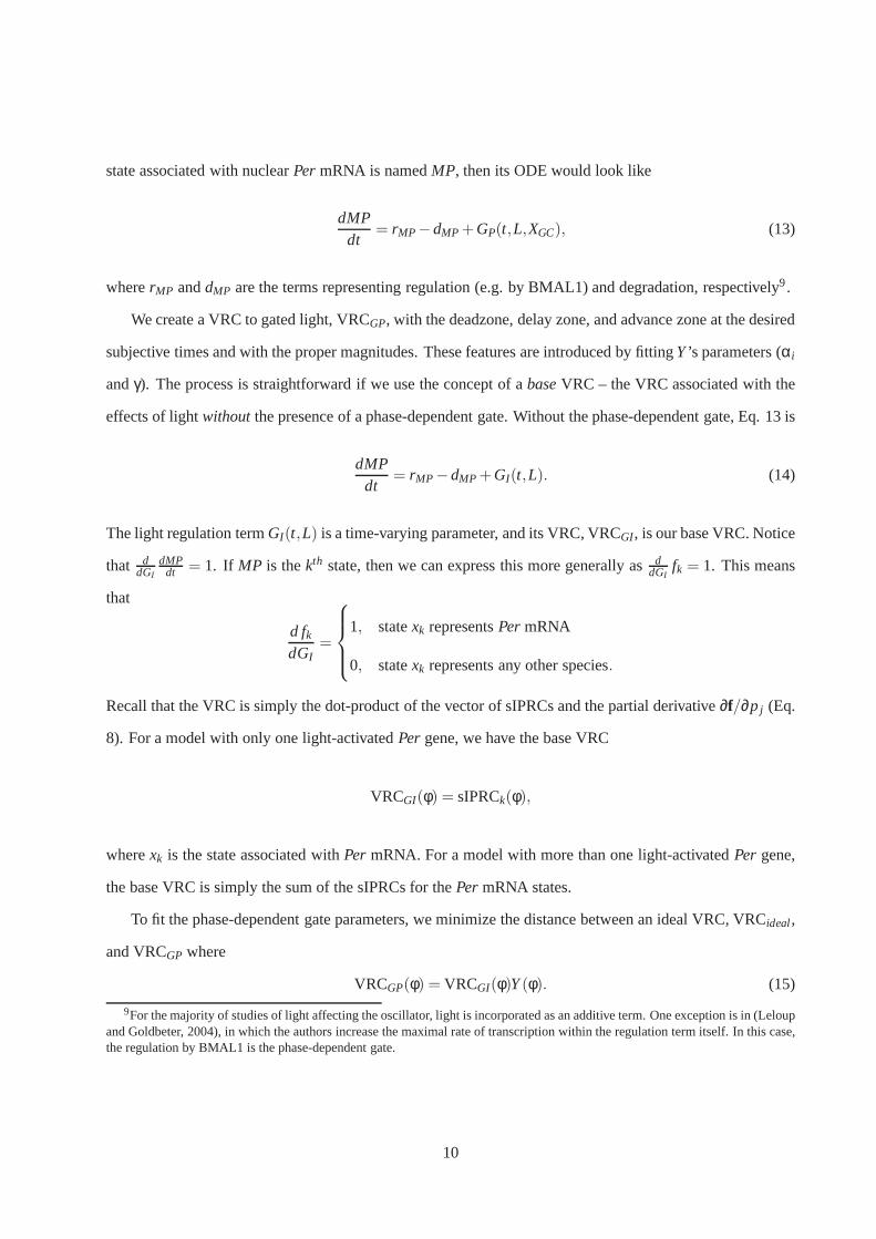
state associated with nuclearPer mRNA is namedMP, then its ODE would look like
dMPdt
= rMP −dMP + GP(t,L,XGC), (13)
whererMP anddMP are the terms representing regulation (e.g. by BMAL1) and degradation, respectively9.
We create a VRC to gated light, VRCGP, with the deadzone, delay zone, and advance zone at the desired
subjective times and with the proper magnitudes. These features are introduced by fittingY ’s parameters (αi
andγ). The process is straightforward if we use the concept of abase VRC – the VRC associated with the
effects of lightwithout the presence of a phase-dependent gate. Without the phase-dependent gate, Eq. 13 is
dMPdt
= rMP −dMP + GI(t,L). (14)
The light regulation termGI(t,L) is a time-varying parameter, and its VRC, VRCGI, is our base VRC. Notice
that ddGI
dMPdt = 1. If MP is thekth state, then we can express this more generally asd
dGIfk = 1. This means
that
d fk
dGI=
1, statexk representsPer mRNA
0, statexk represents any other species.
Recall that the VRC is simply the dot-product of the vector ofsIPRCs and the partial derivative∂f/∂p j (Eq.
8). For a model with only one light-activatedPer gene, we have the base VRC
VRCGI(φ) = sIPRCk(φ),
wherexk is the state associated withPer mRNA. For a model with more than one light-activatedPer gene,
the base VRC is simply the sum of the sIPRCs for thePer mRNA states.
To fit the phase-dependent gate parameters, we minimize the distance between an ideal VRC, VRCideal,
and VRCGP where
VRCGP(φ) = VRCGI(φ)Y (φ). (15)
9For the majority of studies of light affecting the oscillator, light is incorporated as an additive term. One exception is in (Leloupand Goldbeter, 2004), in which the authors increase the maximal rate of transcription within the regulation term itself. In this case,the regulation by BMAL1 is the phase-dependent gate.
10

Phase Response Curves
To compute the phase shift resulting from a light signalL(t) with onset at phaseφ1, we employ one of the
following methods:
• Full Model Method – Perform a numerical experiment with the full model. Compare the position
of a marker (such as the peak ofPer mRNA) in the reference trajectory to that in a simulation with
a w-hour light pulse. For example, if the two trajectories share the same initial conditions and the
experimental trajectory returns to the limit cycle by the tenth cycle, then we compute the phase shift
usingtre f (the time of the peak ofPer mRNA in the tenth cycle of the reference trajectory) andtexp
(the time of the peak in the tenth cycle of the experimental trajectory) according to
PRC(φ1) = texp − tre f . (16)
• Phase Evolution Method – Solve the phase evolution equation(Eq. 7) in the presence of the light
pulse. Compare the phase to zeitgeber time at the end of the simulation, according to
PRC(φ1) = φ(tend)− tend . (17)
• Method of Averaging – Use the VRC with the method of averaging. Compute the PRC10 with GI(t,L)
and VRCGP via
PRC(φ1) =
Z τ
0VRCGP(t + φ1)GI(t,L)dt. (18)
For more details, see (Taylor et al., 2008).
Entrainment
Phase Angle of Entrainment
The phase angle of entrainment relates the phase of the clockto the zeitgeber, e.g. the dawn phase angle
of entrainment is the phase of the entrained clock when it encounters the onset of light each day. Given a
light/dark patternLD, where the photoperiod lastsw hours, the phase angle of entrainmentψ is predicted
10Computing the PRC with the method of averaging is similar to calculating the interaction functionH in (Kuramoto, 1984).
11

by the PRC. For a natural photoperiod, we compute the dawn phase angle of entrainmentψBL and the dusk
phase angle of entrainmentψEL.
• If PRC(φ) is the phase shift incurred by a light pulsebeginning at phaseφ and lastingw hours, then
ψBL is the phase such that PRC(ψBL) = τ−T and the slope of the PRC is negative atψBL.
• If PRCo f f set(φ) represents the phase shift incurred by aw-hour light pulseending at phaseφ, ψEL is
the phase such that PRCo f f set(ψEL) = τ−T and the slope of the PRC is negative atψEL. According
to limit cycle theory, phase adjustments are made while the clock is receiving a signal and end when
the signal ends. The state trajectories may still be in transient, but the phase shifting has completed.
Thus the phase of pulse offset must take into account both theduration of the pulse and the shift it
incurs. The offset PRC is computed from the onset PRC according to
PRCo f f set(φ+ w +PRC(φ)) = PRC(φ), for all φ.
Phase Transition Map
The phase transition curve (PTC) describes the phase of the oscillator one cycle after encountering a pulse
of light. It is computed from the PRC for the appropriate pulse of light according to
PTC(φ) = φ+ PRC(φ).
The phase transition map (PTM) describes the phase of the next cycle, but with respect to an entraining
signal of periodT . It is computed from the PTC according to
PTM(φ) = PTC(φ)+ T − τ. (19)
The phase angle of entrainmentψ falls on the intersection of the PTM and the lineφ = φ.
A Closer Look at the VRC Theory of Entrainment
The VRC theory of entrainment states that the rate of internal time (i.e. phase progression) is adjusted con-
tinuously, but that most of the adjustment occurs circa dawnand dusk (Swade, 1969; Daan and Pittendrigh,
12

1976b). Figure 1A shows a theoretical VRC plotted as a function of phase. The response to light is an
adjustment in the speed – during early subjective morning the clock will speed up, during subjective day-
time there is a deadzone with no response, during early subjective evening the clock will slow down, and
during the subjective night the clock will transition from deceleration to acceleration. In the presence of an
entraining light signal, the phase is dynamically adjusting and the VRC is deformed (as is shown for PRCs
by Pittendrigh and Daan (1976) Figure 2).
The VRC illustrates both the differences and similarities between the continuous model of entrainment
and the discrete model. Figures 1B and 1C show the VRC as a function of zeitgeber time of fast clock
(τ = 23.7h) under full photoperiod (LD12:12) and photoskeleton (LD1:10:1:23) entrainment, respectively.
The dawn and dusk phase angles of entrainment are nearly identical despite the different light schedules (in
Figures 1B and C, the VRC values at ZT0 and ZT12 are very close). However, examining the VRC values
throughout the entire daytime reveals the subtle differences in the phase dynamics leading to those phase
angles. In the presence of 12 hours of light, the dynamics areshifted more gradually, most notably during
the period between ZT8 and ZT12. Figure 1D allows us to track the phase dynamics more precisely, plotting
the difference between the clocks’ phases and zeitgeber time. At ZT0, the phase of the system undergoing
full photoperiod entrainment is approximately CT0.1 and the phase of system undergoing photoskeleton
entrainment is approximately CT23.4. Under both scenarios, the phase is adjusted dramatically in the first
hour of light. During the daytime, the phases gradually drift away from zeitgeber time – the slope is positive
because the clock represented here has a short period. The system undergoing full photoperiod entrainment
is adjusted during the last 4 hours of daylight while the system undergoing photoskeleton entrainment is
adjusted only during the dusk light pulse. Thus we see clearly that the continuous model of entrainment can
account for data observed in photoskeleton experiments. Aslong as there is a deadzone during the day, it can
be difficult to discern the difference between continuous and discrete entrainment in short-pulse entrainment
experiments.
The deadzone also plays an important role in conserving the phase angle of entrainment over different
photoperiods. As in the discrete theory (Pittendrigh and Daan, 1976), the VRC theory holds that short-
period clocks (those in nocturnal animals) conserve the dusk phase angle under different photoperiods and
that long-period clocks (those in diurnal animals) conserve the dawn phase angle. Figure 1B illustrates how
a short-period clock can conserve its dusk phase for photoperiods of 12 hours or less. In LD12:12, we see
that the photoperiod ranges from just before the deadzone, across the deadzone, and well into the delay zone
13
0 6 12 18 24−3
−2
−1
0
1
2
3
CT
Vel
ocity
Res
pons
eA
8 10 12 14 16
0
6
12
18
Photoperiod (h)
ψ
C
0 6 12 18 24−3
−2
−1
0
1
2
3
CT
Vel
ocity
Res
pons
e
B
8 10 12 14 16
0
6
12
18
Photoperiod (h)
ψ
D
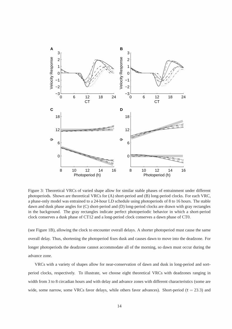
Figure 3: Theoretical VRCs of varied shape allow for similarstable phases of entrainment under differentphotoperiods. Shown are theoretical VRCs for (A) short-period and (B) long-period clocks. For each VRC,a phase-only model was entrained to a 24-hour LD schedule using photoperiods of 8 to 16 hours. The stabledawn and dusk phase angles for (C) short-period and (D) long-period clocks are drawn with gray rectanglesin the background. The gray rectangles indicate perfect photoperiodic behavior in which a short-periodclock conserves a dusk phase of CT12 and a long-period clock conserves a dawn phase of CT0.
(see Figure 1B), allowing the clock to encounter overall delays. A shorter photoperiod must cause the same
overall delay. Thus, shortening the photoperiod fixes dusk and causes dawn to move into the deadzone. For
longer photoperiods the deadzone cannot accommodate all ofthe morning, so dawn must occur during the
advance zone.
VRCs with a variety of shapes allow for near-conservation ofdawn and dusk in long-period and sort-
period clocks, respectively. To illustrate, we choose eight theoretical VRCs with deadzones ranging in
width from 3 to 8 circadian hours and with delay and advance zones with different characteristics (some are
wide, some narrow, some VRCs favor delays, while others favor advances). Short-period (τ = 23.3) and
14

long-period (τ = 24.7) clocks with each of these VRCs entrain to 24-hour cycles with photoperiods ranging
from 8 to 16 hours. We show the VRCs and the dawn and dusk phase angles for a short-period clock in
Figures 3A and 3C. In Figures 3B and 3D, we show the same for a long-period clock. The VRCs in the
two upper panels are identical in shape, but are aligned to allow for the dawn phase angle of entrainment
under LD12:12 to be CT0. Regardless of the precise shape of the VRC, short-period animals conserve the
dusk phase (gaining at most 2.5 hours) and long-period animals conserve the dawn phase (losing at most 3.9
hours). Of the prominent characteristics (area under the delay and advance sections, slopes of the delay and
advance sections, width of the advance, delay, and deadzones, and maximal delays and advances), only the
deadzone width indicates the degree of phase angle conservation – the longer the deadzone, the better the
conservation.
Results
The ideal VRC to light will cross zero with positive slope in the subjective evening (circa CT15-CT18).
The positive-slope zero-crossings of four published mammalian models are CT0.2 (Forger and Peskin,
2003), CT11.8 (Leloup and Goldbeter, 2003), CT15.6 (a modified Goodwin oscillator) (Gonze et al., 2005),
and CT15.7 (Becker-Weimann et al., 2004). We incorporate both light gates into the latter two models,
designing the phase-dependent gate to produce a VRC similarto that of the nocturnal animal model in
(Geier et al., 2005). For the modified Goodwin oscillator, the phase dependent gateGP (Eq. 12) uses
XGC(x) = 0.5417x2 + 0.9784x3, A = 2.2155, andB = 2.4506. For the 7-state model of Becker-Weimann
(2004), GP (Eq. 12) usesXGC(x) = 0.2x3, A = 1.5326, andB = 1.8701. As in (Geier et al., 2005), we
scale the rate constants to acquire a free-running periodτ of 23.7 hours. We label the former model MGG
(Modified Goodwin with Gate) and the latter BWG (Becker-Weimann with Gate).
The PRCs for these two models are computed for light pulses ofdurations 1, 3, 4, 6, 9, 12, and 18 hours,
as in (Comas et al., 2006). Figure 4 shows the PRCs for BWG computed via A) the full model method, B)
the phase evolution method, and C) the method of averaging. We align them according to the approximate
circadian time of the center of the pulse (again, as in (Comaset al., 2006)). The results are similar for MGG
(data not shown).
To evaluate the VRC theory of entrainment, we study the process of re-entrainment when the clock is
out of phase with the environment. We perform numerical experiments mimicking those most commonly
15
performed in behavioral experiments, i.e. single pulse entrainment, full photoperiod entrainment, and pho-
toskeleton entrainment experiments. To begin, we attempt to entrain the clock models with a daily LD
schedule of 1:2311 and find that MGG does not entrain. Even after a stable phase ofentrainment seems
to be achieved, the amplitude of oscillations continues to vary. Thus for the remainder of the experiments
“the model” refers to BWG. The entrainment experiments for this model useL = 1.5 to indicate “lights on”
and are initiated from 25 initial conditions, covering the entire cycle (i.e. we associate the onset of light
in zeitgeber time (ZT0) with CT0, CT1, CT2, etc.). We predictthe stable phase of entrainment using the
full model 1-hour PRC (Figure 5A, top panel) asψBL =CT11. All experiments converge to an actual stable
phase angle of entrainmentψBL=CT10.7, with the time to convergence dependent upon the initial phase dif-
ference between circadian time and zeitgeber time. In the lower panel of Figure 5A, we show the number of
cycles required to reset the clock to within 15 minutes ofψBL versus the circadian time associated with ZT0.
To examine the process of entrainment, we plot the phase transitions for three experiments (ZT0 associated
with CT6, CT12, and CT18) on the phase transition map (PTM) computed from the full model PRC (Figure
5B). For each circle, its x-axis position is its phase at the onset of light (φBL) of cyclei and its y-axis position
is its phase at the onset of light of cyclei+1. The circles are connected to clarify the process from cycle to
cycle. The clocks in the ZT0=CT6 and ZT0=CT18 experiments reachψBL by advancing their phase daily,
while the ZT0=CT12 experiment’s clock delays its phase daily. Figure 5C summarizes the results of all
experiments by showing the phase of the clock at the onset of light each day.
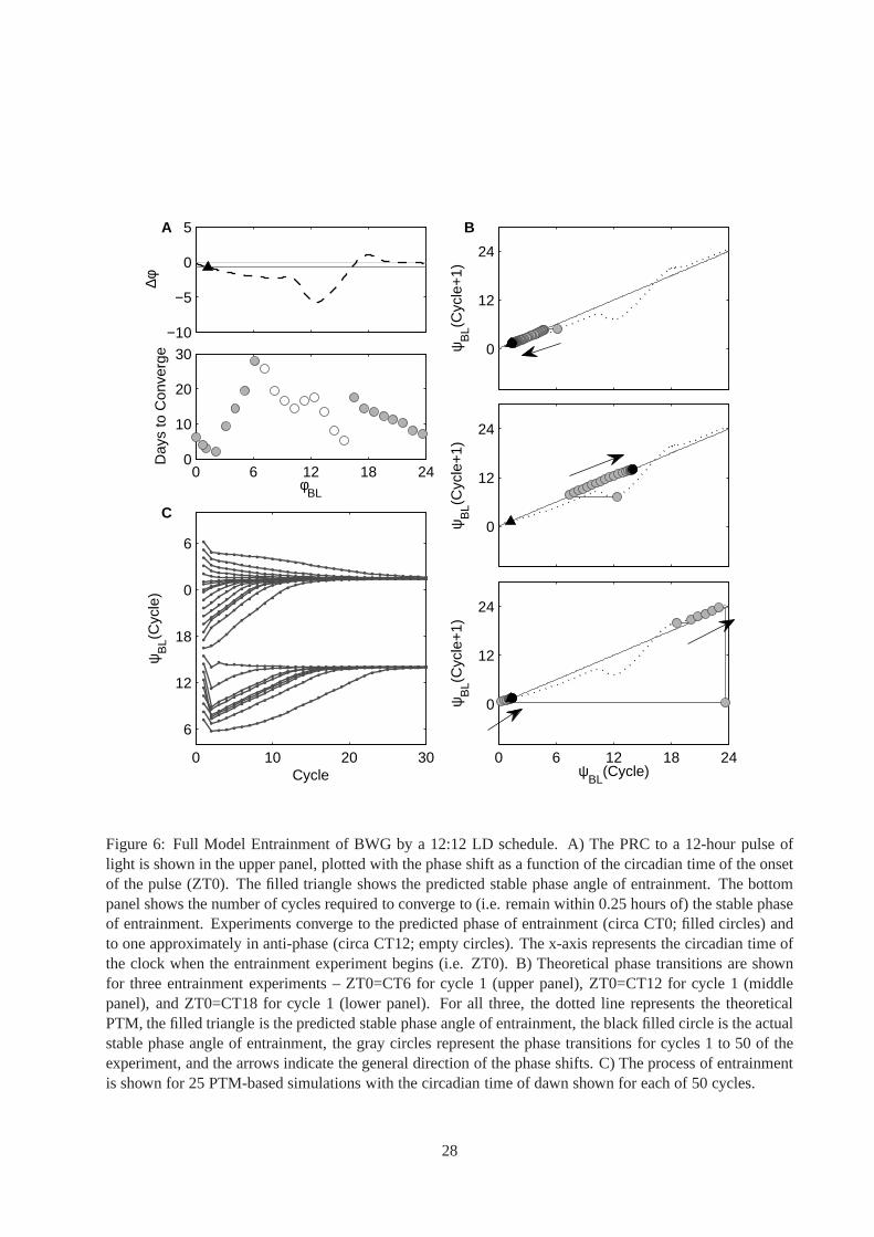
To examine the effects of a full photoperiod, we entrain the clock with an LD schedule of 12:12. The
entrainment experiments are initiated from 25 initial conditions, covering the entire cycle (i.e. we associate
ZT0 with CT0, CT1, CT2, etc.). We predict the stable phase of entrainment using the full model 12-hour
PRC (Figure 6A, top panel) asψBL=CT1.3. Some experiments converge to an actual stable phaseangle of
entrainmentψBL=CT1.5, while others converge toψBL=CT14. In the lower panel of Figure 6A, we show
the number of cycles required to reset the clock to within 15 minutes ofψBL versus the circadian time asso-
ciated with ZT0. The experiments converging to the predicted ψBL are shown with filled circles and those
converging toψBL=CT14 are shown with empty circles. Like above, we plot the phase transitions for three
experiments (ZT0 associated with CT6, CT12, and CT18) on thePTM computed from the full model PRC
(Figure 6B). The clocks in the ZT0=CT6 and ZT0=CT18 experiments reach theψBL by advancing their
phase daily, while the ZT0=CT12 experiment’s clock delays its phase on the first day and advances it the
11That, is a daily light/dark schedule of 1 hour of light followed by 23 hours of dark.
16

remaining days. We examine the state trajectories for all experiments and find that, for experiments con-
verging to the predicted phase of entrainment, all entrained state trajectories are similar to their trajectories
in constant darkness. In contrast, the experiments entraining to an incorrect phase show state trajectories
deviating significantly from their cycle in constant darkness (data not shown).
To further investigate the entrainment process with a full photoperiod, we turn to a phase-only system
in which we use the PTM directly to determine the daily changes in phase. As above, the entrainment
experiments are initiated from 25 initial conditions and the PTM is computed from the full model 12-hour
PRC. Figure 7A shows the 12-hour PRC and the time to convergence. Again we plot the phase transitions
for three experiments (ZT0 associated with CT6, CT12, and CT18) on the PTM computed from the full
model PRC (Figure 7B). The clocks in the ZT0=CT6 and ZT0=CT12scenarios reach theψBL by delaying
their phase daily, while the ZT0=CT18 scenario’s clock advances daily. Figure 7C summarizes the results.
To compare the full photoperiood to the skeleton photoperiod, we repeat the experiments for a LDLD
schedule of 1:10:1:12. To predict the stable phase of entrainment, we compute a phase response curve (via
the full model method) to a light pattern LDL=1:10:1. There are two theoretical stable phase angles of
entrainment (Figure 8A) asψBL =CT23.7 (i.e. the first light pulse is associated with dawn) and CT11 (i.e.
the second light pulse is associated with dawn). In Figure 8B, we show the number of cycles required to
reset the clock to within 15 minutes ofψBL versus the circadian time associated with ZT0. Experiments
converge toψBL =CT23.4 (filled circles) and toψBL=CT10.7 (empty circles). As with the 1-hour single
pulse entrainment experiments, the system remains on the PTM throughout the process of entrainment (data
not shown).
Finally, we study the dawn and dusk phases of entrainment under 24-hour LD cycles with photoperiods
of 8, 9, 10, 11, 12, 13, 14, 15, and 16 hours. First, using a phase-only model (Eq. 7) with the full model’s
VRC (shown in Figure 9A), we predict the dawn and dusk phase angles. The predicted dawn anglesψBL are
CT5.7, CT4.7, CT3.6, CT2.6, CT1.6, CT0.53, CT23.5, CT22.5,and CT21.4, respectively. The predicted
dusk angleψEL is CT13.2 for all photoperiods. Next, we use the full model PRCs for 8- to 16-hour pulses
of lights. We predictψBL will be CT5.3, CT4.3, CT3.3, CT2.2, CT1.2, CT0.2, CT23.5, CT22.2, and CT21.2
(see Figure 9B). The dusk phase anglesψEL are predicted to be CT12.9 for photoperiods of 8 to 13 hours and
CT13 for photoperiods of 14 to 16 hours (see Figure 9C). Afterentraining the full model, the observed dawn
phase angles are CT5.6, CT4.5, CT3.5, CT2.5, CT1.5, CT0.4 CT23.4, CT22.4, and CT21.3, respectively.
The dusk phase angle is always CT13.
17

Discussion
The gated Becker-Weimann model entrains to LD schedules with a stable wave form and is the model
we consider for the remainder of paper, refering to it as “themodel.” Its PRCs (computed with the full
model method) closely match the data in (Comas et al., 2006).The trends in phase evolution and averaging
predictions are correct as well. Together these data show that modeling the correct velocity response curve
is, at least for this model, sufficient for predicting the longterm response to differing light signals. This
is significant because the PRC shapes change as the duration of light increases. The model PRC displays
an increase in the delay to advance ratio. As is typical for a nocturnal animal, the PRC to a one-hour
light pulse produces an area under the delay region,D, greater than the area under its advance region,
A. Comas et al. observed that|A−D| grew with pulse duration and postulated that the reverse might be
seen in PRCs collected for typical diurnal animals (i.e.A > D in the 1-hour PRC). With the method of
averaging, it is relatively straight forward to show that this should be the case and thatA−D is proportional
to w ·R τ
0 VRC(φ)dφ. The agreement between full model PRCs and phase-only PRCs also support conclusions
drawn from previously published phase-only models (Comas et al., 2006; Comas et al., 2007) that longer-
duration PRCs can be predicted from short-duration pulse PRCs. Here, we are assuming not that the 1-hour
PRC is the basis for computation, but that the VRC, an infinitesimally short pulse PRC, is the basis for
computation.
Our simulations show that the steady-state response of the model is biologically realistic, but that this is
no guarantee that it will re-entrain properly from all initial phase mismatches. In other words, demonstrating
the correct long-term response is not equivalent to demonstrating the correct short-term (24-hour) response.
The full model shows a realistic short-term response and re-entrains to the correct phase angleψBL if the
model returns promptly to the DD limit cycle during each scotoperiod. For the 9 full photoperiod simulations
that result in an incorrectψBL, the entrained cycle differs significantly from the DD limitcycle.
After a 1-hour pulse of light, the model does return to the DD limit cycle, and simulations using these
pulses are realistic on several levels. First, all methods of 1-hour pulse PRC computation produce nearly
identicalin silico experimental PRCs, which are, in turn, very similar toin vivo (behavioral) PRCs. Second,
the numerical experimental entrainment process flows according to the theoretical PTM, a process which,
again, is a reasonable description of the process of entrainment seen in behavioral experiments. The data
in Figure 5 provide additional support for the hypothesis ofWatanabe et al. (2001) that resetting is accom-
18

plished within the first day even when the output indicates a lag. In addition, it supports conclusions from
two-pulse experiments such as those by Best et al. (1999), which indicate that resetting is accomplished
within two hours. In our data it is clear that the phase shift is completed before the end of the cycle at all
sections of the curve; the data from all cycles in all experiments aligns with the PTM (see Figure 5B; three
are shown, but the statement is true for all).
In natural light/dark cycles, we expect to see phase velocity increase in the early morning, no adjust-
ments made during the deadzone, and then phase velocity decrease in the early evening. The overall phase
adjustment is captured by the 12-hour PRC which should then be used to predict the process of entrainment
from cycle to cycle. The 12-hour PRC is used to compute the PTMfor the full photoperiod entrainment
simulations. Our data show that the PTM consistently predicts realistic re-entrainment (see Figure 7), but
that the full model simulations are realistic only when the model returns quickly to the DD limit cycle. For
entrainment simulations beginning in the ranges CT0 to CT6 and CT16 to CT24, the full model simulations
return to the DD limit cycle relatively quickly, follow the PTM, and entrain realistically. For example, these
data show a correct phase angle of entrainment and converge within a week (Yamazaki et al., 2000). It is sig-
nificant that the process of re-entrainment from an animal/environment mismatch follows the PTM because
it demonstrates the ability of the clock to be adjusted continuously by light repeatedly and for that action
to be predictable and effective at re-entrainment. This provides direct support for the VRC dictating phase
response behavior of the clock and the contention that dawn and dusk light transitions play no special role
in entrainment. This is consistent with recent step-PRC experiments, the results of which can be sufficiently
explained by the continuous theory, but not by the discrete (Comas et al., 2008).
The relationship between the discrete and continuous theories can be further understood by compar-
ing PRCs and entrainment for full photoperiods to those for skeleton photoperiods. Both the 12-hour PRC
(Figure 7A, upper panel) and the two-pulse 1:10:1 PRC (Figure 8A) predict dawn stable phase angles of
entrainment relatively close to CT0 (CT23.7 for the photoskeleton and CT1.3 for the photoperiod). This is
readily explained by presence of a deadzone in the VRC – if light is unable to change the clock’s velocity
during the middle of the daytime, then we expect the phase of entrainment to be similar whether or not
light is actually shone on the clock in the middle of the day. The difference in photoskeleton and photope-
riod entrainment is seen in experiments beginning from large mismatches between mouse and environment
phases. Only the photoskeleton PRC predicts two stable phase angles, one in which the 10-hour period of
darkness is considered the “daytime” and the other in which the 12-hour period of darkness is considered
19

the “daytime.” This is consistent with behavioral experiments (Pittendrigh and Daan, 1976). Thus, despite
the predictive power of the skeleton photoperiod, the full photoperiod is required to ensure that the clock
re-entrains in such a way thatPer mRNA peaks during the day.
The relationship between the VRC, the free-running period,and the zeitgeber predicts the stable phase
of entrainment. Our simulations entrain such that the dawn and dusk phases of entrainment are accurately
predicted by the VRC-based phase-only model. First, the free-running period is short, which means we
expect the dusk phase of entrainment to be conserved over changing photoperiods. The deadzone for this
model is 14 hours wide, allowing it to conserve the dusk phaseangle not just over short photoperiods,
but over long photoperiods as well. Figure 9A demonstrates the phase relationship between photoperiods
of increasing duration and the clock. All photoperiods encounter the same section of the delay zone, and
extend as far as necessary into the deadzone. This highly intuitive behavior is also predicted by PRCs to long
pulses of light (see Figures 9B and 9C). A long deadzone allows a short-period clock to perfectly conserve
its dusk phase of entrainment – a feature advantageous to a nocturnal mammal needing to forage at dusk.
When only approximate conservation of dusk is necessary, a deadzone as short as 3 hours may be sufficient
(see Figure 3).
In summary, discrete and continuous entrainment are unifiedby the VRC and can be studied using both
the VRC and the PRC to long pulses of light. Further, much of the intuition developed under the discrete
theory can be transferred directly to the continuous theory. For example, straight-forward prediction of
the phase angle of entrainment – a hallmark of the discrete theory – is also possible within the VRC-
unified theory. In addition, we have shown that the presence of a deadzone is important both functionally
and theoretically. Functionally, the deadzone allows short-period clocks to conserve the dusk phase angle
of entrainment. Theoretically, examining the deadzone reveals why it is difficult to distinguish between
continuous and discrete effects using short pulses of light(see Figure 1). Finally, the implication of this
work is not only a call for more experimentation with long light pulses (such as those of similar to those of
Comas et al. (2006; 2007; 2008)) but also a re-examination ofshort-pulse experiments in light of continuous
theory. Collection of a VRC would be ideal, but is not straight-forward. However, we suggest phase-only
modeling and careful attention to light gating be used to uncover a good approximate VRC.
20

Acknowledgement
We thank Erik Herzog, Rudiyanto Gunawan, Guillaume Bonnet,and Henry Mirsky for helpful discussions.
This work was supported by the Institute for Collaborative Biotechnologies through grant #DAAD19-03-
D-0004 from the U.S. Army Research Office (FJD), NSF IGERT grant #DGE02-21715 (SRT, FJD, LRP),
NSF/NIH grant #GM078993 (SRT, FJD, LRP), Army Research Office grant #W911NF-07-1-0279 (FJD),
and NIH grant #EB007511 (LRP).
References
Aschoff, J. (1979). Circadian rhythms: influences of internal and external factors on the period measured in
constant conditions.Z Tierpsychol, 49(3):225–249.
Becker-Weimann, S., Wolf, J., Herzel, H., and Kramer, A. (2004). Modeling feedback loops of the mam-
malian circadian oscillator.BiophysJ, 87(5):3023–3034.
Beersma, D. G., Daan, S., and Hut, R. A. (1999). Accuracy of circadian entrainment under fluctuating light
conditions: contributions of phase and period responses.JBiol Rhythms, 14(4):320–329.
Best, J. D., Maywood, E. S., Smith, K. L., and Hastings, M. H. (1999). Rapid resetting of the mammalian
circadian clock.JNeurosci, 19(2):828–835.
Brown, E., Moehlis, J., and Holmes, P. (2004). On the phase reduction and response dynamics of neural
oscillator populations.NeuralComput, 16(4):673–715.
Comas, M., Beersma, D., Hut, R., and Daan, S. (2008). Circadian phase resetting in response to light-dark
and dark-light transitions.JBiol Rhythms, 23(5):425–434.
Comas, M., Beersma, D., Spoelstra, K., and Daan, S. (2007). Circadian response reduction in light and
response restoration in darkness: a “skeleton” light pulsePRC study in mice (Mus musculus).J Biol
Rhythms, 22(5):432–444.
Comas, M., Beersma, D. G. M., Spoelstra, K., and Daan, S. (2006). Phase and period responses of the cir-
cadian system of mice (Mus musculus) to light stimuli of different duration.JBiol Rhythms, 21(5):362–
372.
Daan, S. and Pittendrigh, C. S. (1976a). A functional analysis of circadian pacemakers in nocturnal rodents.
ii. the variability of phase response curves.JCompPhysiol, 106(3):253–266.
21

Daan, S. and Pittendrigh, C. S. (1976b). A functional analysis of circadian pacemakers in nocturnal rodents.
iii. heavy water and constant light: Homeostasis of frequency? JCompPhysiol, 106(3):267–290.
Forger, D. B. and Peskin, C. S. (2003). A detailed predictivemodel of the mammalian circadian clock.Proc
Natl AcadSci U S A, 100(25):14806–14811.
Geier, F., Becker-Weimann, S., Kramer, A., and Herzel, H. (2005). Entrainment in a model of the mam-
malian circadian oscillator.JBiol Rhythms, 20(1):83–93.
Gonze, D., Bernard, S., Waltermann, C., Kramer, A., and Herzel, H. (2005). Spontaneous synchronization
of coupled circadian oscillators.BiophysJ, 89(1):120–129.
Johnson, C. H., Elliott, J. A., and Foster, R. (2003). Entrainment of circadian programs.ChronobiolInt,
20(5):741–774.
Khammanivong, A. and Nelson, D. E. (2000). Light pulses suppress responsiveness within the mouse photic
entrainment pathway.JBiol Rhythms, 15(5):393–405.
Kramer, M., Rabitz, H., and Calo, J. (1984). Sensitivity analysis of oscillatory systems.Appl Math Mod,
8:328–340.
Kuramoto, Y. (1984).Chemicaloscillations,waves,andturbulence. Springer-Verlag, Berlin.
Leloup, J.-C. and Goldbeter, A. (2003). Toward a detailed computational model for the mammalian circadian
clock. ProcNatl AcadSci U S A, 100(12):7051–7056.
Leloup, J.-C. and Goldbeter, A. (2004). Modeling the mammalian circadian clock: sensitivity analysis and
multiplicity of oscillatory mechanisms.J theorBiol, 230(4):541–562.
Nelson, D. E. and Takahashi, J. S. (1999). Integration and saturation within the circadian photic entrainment
pathway of hamsters.Am JPhysiolRegulIntegrCompPhysiol, 277(5):R1351–R1361.
Peterson, E. L. (1980). A limit cycle interpretation of a mosquito circadian oscillator. J theor Biol,
84(2):281–310.
Pittendrigh, C. S. and Daan, S. (1976). A functional analysis of circadian pacemakers in nocturnal rodents.
iv. entrainment: Pacemaker as clock.JCompPhysiol, 106(3):291–331.
Reppert, S. M. and Weaver, D. R. (2001). Molecular analysis of mammalian circadian rhythms.Annu Rev
Physiol, 63:647–676.
Roenneberg, T., Daan, S., and Merrow, M. (2003). The art of entrainment.JBiol Rhythms, 18(3):183–194.
Swade, R. H. (1969). Circadian rhythms in fluctuating light cycles: toward a new model of entrainment.J
theorBiol, 24(2):227–239.
22

Taylor, S. R., Gunawan, R., Petzold, L. R., and Doyle III, F. J. (2008). Sensitivity measures for oscillating
systems: Application to mammalian circadian gene network.IEEE TransAutomatContr, 153(Special
Issue):177–188.
Watanabe, K., Deboer, T., and Meijer, J. H. (2001). Light-induced resetting of the circadian pacemaker:
quantitative analysis of transient versus steady-state phase shifts.JBiol Rhythms, 16(6):564–573.
Winfree, A. T. (2001).TheGeometryof Biological Time. Springer, New York.
Yamazaki, S., Numano, R., Abe, M., Hida, A., Takahashi, R., Ueda, M., Block, G. D., Sakaki, Y., Menaker,
M., and Tei, H. (2000). Resetting central and peripheral circadian oscillators in transgenic rats.Science,
288(5466):682–685.
Figure Legends
Figure 1. Velocity response curves (VRCs) in free-run and under entrainment. A) The VRC has a shape
similar to that of a PRC, but shows changes in the clock’s velocity. When the VRC is one, then light (L = 1)
doubles the speed of the clock. The VRC is shown as its changesunder B) full photoperiod (12:12) and C)
skeleton photoperiod (1:10:1:12) entrainment. D) Shown isthe difference between zeitgeber time and the
phase of the clock under both entrainment scenarios (solid line for the full photoperiod, dashed line for the
skeleton photoperiod). Positive values indicate the internal phase is ahead of zeitgeber time. The dark gray
background indicates night in both scenarios. The light gray background from ZT1 to ZT11 indicates the
period of darkness during photoskeleton entrainment.
Figure 2. Input Schematic. Light gates are shown as rectangles, the core clock as a circle, and input and
feedback are shown as arrows. The external light cueL passes through the initial gate, which produces an
attenuated light signalGI(L). This signal then passes through the phase-dependent gate,which uses clock
componentsXGC to compute further signal attenuation. The result isGP(GI(L),XGC), which manipulates
the core clockX . The core clock sends output signals to peripheral oscillators which, in turn, may feed back
to the clock. The output processes are shown in gray and are not included in the models under consideration.
Figure 3. Theoretical VRCs of varied shape allow for similar stable phases of entrainment under dif-
ferent photoperiods. Shown are theoretical VRCs for (A) short-period and (B) long-period clocks. For each
VRC, a phase-only model was entrained to a 24-hour LD schedule using photoperiods of 8 to 16 hours.
The stable dawn and dusk phase angles for (C) short-period and (D) long-period clocks are drawn with
23

gray rectangles in the background. The gray rectangles indicate perfect photoperiodic behavior in which a
short-period clock conserves a dusk phase of CT12 and a long-period clock conserves a dawn phase of CT0.
Figure 4. Phase Response Curves for the Becker-Weimann model with both gates. PRCs calculated
with A) the full model method, B) the phase evolution method,and C) the method of averaging are shown
for light pulses of durations 1, 3, 4, 6, 9, 12, and 18 hours. The phase shift is plotted as a function of the
circadian time of the middle of the pulse.
Figure 5. Full Model Entrainment of BWG by a 1:23 LD schedule. A) The PRCto a 1-hour pulse of
light is shown in the upper panel, plotted with the phase shift as a function of the circadian time of the onset
of the pulse (ZT0). The filled triangle shows the predicted stable phase angle of entrainment (with respect
to pulse onset). The bottom panel shows the number of cycles required to converge to (i.e. remain within
0.25 hours of) the stable phase of entrainment. The x-axis represents the circadian time of the clock when
the entrainment experiment begins (i.e. the onset ZT0 of thefirst light pulse). B) The phase transitions
are shown for three entrainment experiments – ZT0=CT6 for cycle 1 (upper panel), ZT0=CT12 for cycle
1 (middle panel), and ZT0=CT18 for cycle 1 (lower panel). Forall three, the dotted line represents the
theoretical PTM, the filled triangle is the predicted stablephase angle of entrainment, the black filled circle
is the actual stable phase angle of entrainment, the gray circles represent the phase transitions for cycles 1
to 50 of the experiment, and the arrows indicate the general direction of the phase shifts. C) The process of
entrainment is shown for 25 experiments with the circadian time of dawn shown for each of the 50 cycles.
Figure 6. Full Model Entrainment of BWG by a 12:12 LD schedule. A) The PRC to a 12-hour pulse of
light is shown in the upper panel, plotted with the phase shift as a function of the circadian time of the onset
of the pulse (ZT0). The filled triangle shows the predicted stable phase angle of entrainment. The bottom
panel shows the number of cycles required to converge to (i.e. remain within 0.25 hours of) the stable phase
of entrainment. Experiments converge to the predicted phase of entrainment (circa CT0; filled circles) and
to one approximately in anti-phase (circa CT12; empty circles). The x-axis represents the circadian time of
the clock when the entrainment experiment begins (i.e. ZT0). B) Theoretical phase transitions are shown
for three entrainment experiments – ZT0=CT6 for cycle 1 (upper panel), ZT0=CT12 for cycle 1 (middle
panel), and ZT0=CT18 for cycle 1 (lower panel). For all three, the dotted line represents the theoretical
PTM, the filled triangle is the predicted stable phase angle of entrainment, the black filled circle is the actual
stable phase angle of entrainment, the gray circles represent the phase transitions for cycles 1 to 50 of the
experiment, and the arrows indicate the general direction of the phase shifts. C) The process of entrainment
24

is shown for 25 PTM-based simulations with the circadian time of dawn shown for each of 50 cycles.
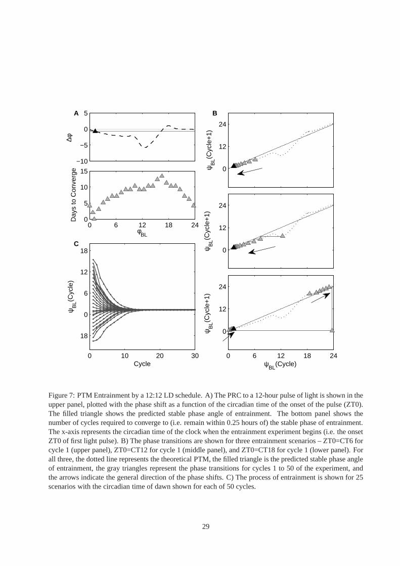
Figure 7. PTM Entrainment by a 12:12 LD schedule. A) The PRC to a 12-hourpulse of light is
shown in the upper panel, plotted with the phase shift as a function of the circadian time of the onset of the
pulse (ZT0). The filled triangle shows the predicted stable phase angle of entrainment. The bottom panel
shows the number of cycles required to converge to (i.e. remain within 0.25 hours of) the stable phase of
entrainment. The x-axis represents the circadian time of the clock when the entrainment experiment begins
(i.e. the onset ZT0 of first light pulse). B) The phase transitions are shown for three entrainment scenarios
– ZT0=CT6 for cycle 1 (upper panel), ZT0=CT12 for cycle 1 (middle panel), and ZT0=CT18 for cycle 1
(lower panel). For all three, the dotted line represents thetheoretical PTM, the filled triangle is the predicted
stable phase angle of entrainment, the gray triangles represent the phase transitions for cycles 1 to 50 of the
experiment, and the arrows indicate the general direction of the phase shifts. C) The process of entrainment
is shown for 25 scenarios with the circadian time of dawn shown for each of 50 cycles.
Figure 8. Entrainment of BWG by a 1:10:1:12 LDLD schedule. A) The PRC totwo 1-hour pulses
of light (separated by 10 hours of darkness) is shown, plotted with the phase shift as a function of the
circadian time of the onset of the pulse (ZT0). The filled triangles show the two predicted stable phase
angle of entrainment (with respect to the onset of the first pulse). B) Shown are the number of cycles each
experiment required to converge to (i.e. remain within 0.25hours of) the stable phase of entrainment. The
x-axis represents the circadian time of the clock when the entrainment experiment begins (i.e. ZT0).
Figure 9. Entrainment under photoperiods of 8 to 16 hours. (A) The model’s VRC is double-plotted.
The photoperiods (all ending at CT13) are shown in gray rectangles, with lighter grays for longer photope-
riods. (B) The full model PRCs for 8- to 16-hour pulses of light are shown, aligned according to the time of
the pulse onset. The ranges of the predicted dawn phase angles ψBL are indicated with arrows. (C) The full
model PRCs for 8- to 16-hour pulses of light are aligned according to the time of pulse offset. The predicted
dusk phase angleψEL is indicated with an arrow.
25

1 hour 3 hours 4 hours 6 hours
9 hours 12 hours 18 hours
−6
−4
−2
0
2
∆φ (
Circ
adia
n h)
A
−4
−2
0
2
∆φ (
Circ
adia
n h)
B
0 6 12 18 24−2
−1
0
1
2
CT at Mid−Pulse
∆φ (
Circ
adia
n h)
C
Figure 4: Phase Response Curves for the Becker-Weimann model with both gates. PRCs calculated with A)the full model method, B) the phase evolution method, and C) the method of averaging are shown for lightpulses of durations 1, 3, 4, 6, 9, 12, and 18 hours. The phase shift is plotted as a function of the circadiantime of the middle of the pulse.
26

−4
−2
0
2
∆φ
A
0 6 12 18 240
10
20
30
φBL
Day
s to
Con
verg
e
0 10 20 30
18
0
6
12
18
Cycle
ψB
L(Cyc
le)
C
0
12
24
B
ψB
L(Cyc
le+
1)
0
12
24ψ
BL(C
ycle
+1)
0 6 12 18 24
0
12
24
ψBL
(Cycle)
ψB
L(Cyc
le+
1)
Figure 5: Full Model Entrainment of BWG by a 1:23 LD schedule.A) The PRC to a 1-hour pulse of lightis shown in the upper panel, plotted with the phase shift as a function of the circadian time of the onsetof the pulse (ZT0). The filled triangle shows the predicted stable phase angle of entrainment (with respectto pulse onset). The bottom panel shows the number of cycles required to converge to (i.e. remain within0.25 hours of) the stable phase of entrainment. The x-axis represents the circadian time of the clock whenthe entrainment experiment begins (i.e. the onset ZT0 of thefirst light pulse). B) The phase transitionsare shown for three entrainment experiments – ZT0=CT6 for cycle 1 (upper panel), ZT0=CT12 for cycle1 (middle panel), and ZT0=CT18 for cycle 1 (lower panel). Forall three, the dotted line represents thetheoretical PTM, the filled triangle is the predicted stablephase angle of entrainment, the black filled circleis the actual stable phase angle of entrainment, the gray circles represent the phase transitions for cycles 1to 50 of the experiment, and the arrows indicate the general direction of the phase shifts. C) The process ofentrainment is shown for 25 experiments with the circadian time of dawn shown for each of the 50 cycles.
27
−10
−5
0
5
∆φ
A
0 6 12 18 240
10
20
30
φBL
Day
s to
Con
verg
e
0 10 20 30
6
12
18
0
6
Cycle
ψB
L(Cyc
le)
C
0
12
24
B
ψB
L(Cyc
le+
1)
0
12
24
ψB
L(Cyc
le+
1)
0 6 12 18 24
0
12
24
ψBL
(Cycle)
ψB
L(Cyc
le+
1)
Figure 6: Full Model Entrainment of BWG by a 12:12 LD schedule. A) The PRC to a 12-hour pulse oflight is shown in the upper panel, plotted with the phase shift as a function of the circadian time of the onsetof the pulse (ZT0). The filled triangle shows the predicted stable phase angle of entrainment. The bottompanel shows the number of cycles required to converge to (i.e. remain within 0.25 hours of) the stable phaseof entrainment. Experiments converge to the predicted phase of entrainment (circa CT0; filled circles) andto one approximately in anti-phase (circa CT12; empty circles). The x-axis represents the circadian time ofthe clock when the entrainment experiment begins (i.e. ZT0). B) Theoretical phase transitions are shownfor three entrainment experiments – ZT0=CT6 for cycle 1 (upper panel), ZT0=CT12 for cycle 1 (middlepanel), and ZT0=CT18 for cycle 1 (lower panel). For all three, the dotted line represents the theoreticalPTM, the filled triangle is the predicted stable phase angle of entrainment, the black filled circle is the actualstable phase angle of entrainment, the gray circles represent the phase transitions for cycles 1 to 50 of theexperiment, and the arrows indicate the general direction of the phase shifts. C) The process of entrainmentis shown for 25 PTM-based simulations with the circadian time of dawn shown for each of 50 cycles.
28
−10
−5
0
5
∆φ
A
0 6 12 18 240
5
10
15
φBL
Day
s to
Con
verg
e
0 10 20 30
18
0
6
12
18
Cycle
ψB
L(Cyc
le)
C
0
12
24
B
ψB
L(Cyc
le+
1)
0
12
24ψ
BL(C
ycle
+1)
0 6 12 18 24
0
12
24
ψBL
(Cycle)
ψB
L(Cyc
le+
1)
Figure 7: PTM Entrainment by a 12:12 LD schedule. A) The PRC toa 12-hour pulse of light is shown in theupper panel, plotted with the phase shift as a function of thecircadian time of the onset of the pulse (ZT0).The filled triangle shows the predicted stable phase angle ofentrainment. The bottom panel shows thenumber of cycles required to converge to (i.e. remain within0.25 hours of) the stable phase of entrainment.The x-axis represents the circadian time of the clock when the entrainment experiment begins (i.e. the onsetZT0 of first light pulse). B) The phase transitions are shown for three entrainment scenarios – ZT0=CT6 forcycle 1 (upper panel), ZT0=CT12 for cycle 1 (middle panel), and ZT0=CT18 for cycle 1 (lower panel). Forall three, the dotted line represents the theoretical PTM, the filled triangle is the predicted stable phase angleof entrainment, the gray triangles represent the phase transitions for cycles 1 to 50 of the experiment, andthe arrows indicate the general direction of the phase shifts. C) The process of entrainment is shown for 25scenarios with the circadian time of dawn shown for each of 50cycles.
29

0 6 12 18 24−4
−2
0
2
φBL
∆φ
A
0 6 12 18 240
5
10
φBL
Day
s to
Con
verg
e
B
Figure 8: Entrainment of BWG by a 1:10:1:12 LDLD schedule. A)The PRC to two 1-hour pulses of light(separated by 10 hours of darkness) is shown, plotted with the phase shift as a function of the circadian timeof the onset of the pulse (ZT0). The filled triangles show the two predicted stable phase angle of entrainment(with respect to the onset of the first pulse). B) Shown are thenumber of cycles each experiment requiredto converge to (i.e. remain within 0.25 hours of) the stable phase of entrainment. The x-axis represents thecircadian time of the clock when the entrainment experimentbegins (i.e. ZT0).
30

0 6 12 18 24 6 12 18 24−1.5
−1
−0.5
0
0.5
1
CT
Vel
ocity
Res
pons
e
A
0 6 12 18 24−6
−4
−2
0
2
Onset of Pulse (CT)
Pha
se S
hift
B
0 6 12 18 24−6
−4
−2
0
2
Offset of Pulse (CT)
Pha
se S
hift
C
ψEL
ψBL
ψBL
Figure 9: Entrainment under photoperiods of 8 to 16 hours. (A) The model’s VRC is double-plotted. Thephotoperiods (all ending at CT13) are shown in gray rectangles, with lighter grays for longer photoperiods.(B) The full model PRCs for 8- to 16-hour pulses of light are shown, aligned according to the time of thepulse onset. The ranges of the predicted dawn phase anglesψBL are indicated with arrows. (C) The fullmodel PRCs for 8- to 16-hour pulses of light are aligned according to the time of pulse offset. The predicteddusk phase angleψEL is indicated with an arrow.
31