vehicle dynamics of a jumping rallycross car - diva …893827/fulltext01.pdf · vehicle dynamics of...
TRANSCRIPT
Postal address Visiting Address Telephone Telefax Internet KTH Teknikringen 8 +46 8 790 6000 +46 8 790 9290 www.kth.se Vehicle Dynamics Stockholm SE-100 44 Stockholm, Sweden
Vehicle Dynamics of a Jumping Rallycross Car
Emil Sällberg and Robert Ekman
Master Thesis in Vehicle Engineering
Department of Aeronautical and Vehicle Engineering KTH Royal Institute of Technology
TRITA-AVE 2015:41 ISSN 1651-7660

Abstract
This master thesis was performed in collaboration with Öhlins Racing AB. The company provides suspension systems to the automotive industry and to motorsport teams globally. Many of Öhlins’ customers compete in rallycross, a style of competition that generally involves highly modified production cars racing on closed, elevated and mixed surfaced circuits. Rallycross cars generally have an inherent problem and tend to over rotate mid-air after taking off from a jump. The vehicle often lands with a large pitch angle, damaging suspension components or losing valuable time when the driver waits for the vehicle to settle. The request from Öhlins was to analyse this phenomenon.
The scope of the master thesis was to; investigate four different simulation software and choose the most appropriate software to simulate a rallycross car, perform a parameter study to analyse which parameters affect the jumping behaviour of the vehicle and study the force build up in the suspension during the landing phase. The four simulation software investigated were LMS Amesim, CarSim, Adams/Car and a 2D MATLAB model. The models were parameterised with vehicle data acquired from a rallycross car and validated against measured data obtained from tests with the same car. The MATLAB model was considered to be the best performing model given the criteria which were set up.
A parameter study was conducted with the chosen simulation model where different vehicle parameters, driver behaviour and road profiles were analysed to investigate what impact they had on the jumping performance of the rallycross car. It could be concluded that the rear damper stiffness is critical for the jumping behaviour of the vehicle and that a stiffer rear damper generally gives the best performance. The longitudinal position of the centre of gravity also has a significant impact on vehicle jumping where a position in the middle between front and rear axle is preferred.
The force build-up in the vehicle suspension was also analysed. Vehicle jumping and landing behaviour was compared to measurements from a human jumping in order to investigate if a human jumping utilised other force build-up strategies. It was found that the car force build-up during landing was similar to a human beings. Other force build-up strategies for the dampers were tested and it was found that dampers reacting to stroke position or hub acceleration can improve jumping performance of a rallycross car.

Acknowledgements We would like to express our gratitude to Kent Persson and Jonas Jarlmark Näfver, our supervisors at Öhlins Racing, for taking their valuable time to help us and provide reasoning during times of occasional confusion. Many thanks to Lars Drugge, supervisor at KTH, for giving valuable feedback throughout the work. We would also thank the involved rallycross teams and drivers for their involvement during the thesis work and for providing useful vehicle data. Thanks to Patric Jansson, Eric Contreras and Milan Horemuz at The Division of Geodesy and Satellite Positioning at KTH for teaching- and lending us the GPS equipment. We would also like to say thanks to Jan-Ola Persson and Ola Blomgren at Trimble Karlstad for the kind service and the lending of Trimble equipment at such short notice.
Stockholm, April 2015 Emil Sällberg and Robert Ekman


Table of Contents
1 Introduction ......................................................................................................................... 1
1.1 Background ............................................................................................................................. 1
1.2 Problem definition ................................................................................................................... 1
1.3 Objective and delimitation ...................................................................................................... 2
1.4 Software specification ............................................................................................................. 2
2 Preparatory work ................................................................................................................. 3
2.1 Driver interviews ..................................................................................................................... 3
2.2 Measuring race circuits............................................................................................................ 3
2.3 Logged vehicle data ................................................................................................................. 4
2.4 Measuring vertical tyre stiffness ............................................................................................. 4
3 Software introduction .......................................................................................................... 7
3.1 CarSim ..................................................................................................................................... 7
3.2 ADAMS/Car ............................................................................................................................ 8
3.3 LMS Amesim .......................................................................................................................... 9
3.4 MATLAB .............................................................................................................................. 10
3.4.1 Planar motions ............................................................................................................... 10
3.4.2 Longitudinal tyre model ................................................................................................ 11
3.4.3 Driveline model ............................................................................................................. 12
3.4.4 Road model .................................................................................................................... 14
3.4.5 Driver inputs .................................................................................................................. 15
3.4.6 Springs and dampers...................................................................................................... 16
3.4.7 GUI ................................................................................................................................ 18
3.4.8 MATLAB summary ...................................................................................................... 19
4 Simulation model setup ..................................................................................................... 21
4.1 Vehicle properties .................................................................................................................. 21
4.2 Road profile creation ............................................................................................................. 21
4.3 CarSim ................................................................................................................................... 21
4.4 ADAMS/Car .......................................................................................................................... 21
4.5 LMS Amesim ........................................................................................................................ 22
4.6 MATLAB .............................................................................................................................. 22
5 Evaluation of models ........................................................................................................ 23
5.1 Validation .............................................................................................................................. 23
5.1.1 Jump A1 ........................................................................................................................ 23
5.1.2 Jump B ........................................................................................................................... 26
5.1.3 Validation summary ...................................................................................................... 29
5.2 Usability ................................................................................................................................ 29
5.2.1 CarSim ........................................................................................................................... 29
5.2.2 ADAMS/Car .................................................................................................................. 29
5.2.3 Amesim ......................................................................................................................... 30
5.2.4 MATLAB ...................................................................................................................... 30
5.3 Simulation model of choice ................................................................................................... 30
6 Parameter study ................................................................................................................. 31
6.1 Simulation setup .................................................................................................................... 32
6.2 Results ................................................................................................................................... 34
6.2.1 Spring stiffness .............................................................................................................. 34
6.2.2 Damper stiffness ............................................................................................................ 36
6.2.3 Centre of gravity position .............................................................................................. 37
6.2.4 Throttle application and entry speed ............................................................................. 38
6.2.5 Optimised settings ......................................................................................................... 40
6.3 Additional studies .................................................................................................................. 41
6.3.1 Throttle application ....................................................................................................... 41
6.3.2 Entry speed .................................................................................................................... 42
7 Force build up analysis ..................................................................................................... 45
7.1 Human comparison ................................................................................................................ 45
7.2 Force strategies ...................................................................................................................... 46
8 Discussion ......................................................................................................................... 51
8.1 Evaluation of models ............................................................................................................. 51
8.2 Parameter study ..................................................................................................................... 52
8.3 Force build up ........................................................................................................................ 52
9 Conclusion ........................................................................................................................ 55
10 Future work ................................................................................................................... 57
11 References ..................................................................................................................... 59
Appendix A – Vehicle data ................................................................................................. 61
Appendix B – Model validation .......................................................................................... 63
Appendix C – Parameter study ........................................................................................... 65

1
1 Introduction
1.1 Background
This master thesis was done in collaboration with Öhlins Racing AB, situated in Upplands-Väsby, Sweden. Öhlins Racing develops suspension technology and systems for motorsport applications as well as for automotive and motorcycle manufacturers globally. The company was founded by Kenth Öhlin in 1976 as he wanted to develop shock absorbers, also known as dampers, for motocross racing purposes. The company later on developed in to producing shock absorbers for a multitude of motorsport purposes, ranging from motocross and road racing to rally and racing applications.
Rallycross is a form of motorsport which combines rally and racing in a sprint-race format on closed circuits with a mix of gravel and tarmac surfaces. The cars are also a combination of rally and racing cars, as they have to deal with the high grip of tarmac racing and the gravel and jumps of rally. The sport has observed an upswing over the last few years as more manufacturer support has entered the sport, which has increased the need for rallycross car development in general.
The technical regulations of rallycross are fairly open in many classes, giving a lot of leeway for creative modifications to the production vehicle which is most often the base. There are two main classes on a national and international level; Supercar and Supercar Lites.
The Supercar class has production based vehicles with four-wheel drive, typically a front- and longitudinally-mounted turbocharged engine and usually MacPherson or double wishbone suspension. The Supercar Lites are a one-make class where all cars are identical in specification. They have four-wheel drive and a longitudinally mid-mounted 2.4 litre normally aspirated engine, together with double wishbone suspension front and rear.
1.2 Problem definition
One of the main challenges the rallycross teams face is to manage the vehicle jumping behaviour. Cars often tend to over-rotate mid-air after leaving a jump and land hard on the front axle. The impact usually upsets the vehicle and time is lost when the driver waits for it to settle, or the impact might damage the suspension or important structure and components around the front axle. Customer teams seek support from Öhlins in this matter and there is a desire from the company to gain more knowledge in this area.
The request from Öhlins was to; investigate a predetermined set of simulation software for modelling jumping behaviour of rally cross cars, investigate what parameters affect the dynamics of the vehicle during the jumping phase and analyse the force build up in the suspension during landing. The software investigated were ADAMS/Car, LMS Amesim, CarSim and MATLAB.
The variables to be analysed in the parameter study were vehicle properties that can be tuned by changing suspension components such as damper and spring stiffness, but also

2
parameters that only can be affected by the vehicle manufacturer, such as the position of the centre of gravity. It is also known from experience that driver behaviour affects the jumping dynamics of the vehicle and therefore throttle application and jump entry speed are investigated.
1.3 Objective and delimitation
The purpose of this master thesis is to;
• Investigate four different simulation tools to find the most suitable one for solving the specific problem, with respect to a given set of criteria
• Analyse the change in jumping behaviour when altering vehicle parameters • Analyse force build up in the vehicle suspension during landing
Due to time constraints, the scope of the master thesis is narrowed down and the delimitations of the project are;
• Simulations are refrained to 2D vehicle modelling, x-z plane. • Only a specific type of rallycross vehicle will be analysed • Settle time and energy absorption in the suspension and tyres during landing are
the main factors that will be analysed in the parameter study
1.4 Software specification
Criteria for the software were set up together with Öhlins. In order for the software to be fully exploitable by the company, it should;
• Be user friendly • Require low expenditure of time to set up the model and simulate it • Accurately predict vehicle behaviour • Give the possibility to develop the simulation model and extend the vehicle
library
In terms of user friendliness, Öhlins had specified that a vehicle engineer, with no previous experience of the software, should be able to set up a new model, use it to run simulations, analyse the results and assist in reaching accurate conclusions regarding the simulated vehicle behaviour within the scope of one day. Another requirement was that the simulation model had to be adaptable to allow for implementation of new damper types which characteristics e.g. not solely based on stroke speed.
The assessment of the software in terms of user friendliness was based on subjective reasoning. Emphasis was put on how intuitive the software are with respect to; model parametrisation, road profile creation and result management. The authors of this report have no previous experience from CarSim and LMS Amesim. Some experience from ADAMS/Car has been obtained through university courses while MATLAB has been used frequently during the entire education.
The software were validated with respect to wheel displacement and wheel displacement speed as well as time of impact on front and rear axle respectively. The latter is used as an indication of the pitch behaviour of the simulated vehicle.

3
2 Preparatory work
Some preparatory work were carried out before investigating the simulation models. Three rallycross drivers and one engineer were interviewed in regard to the issue of vehicle handling during the jumping phase. The goal was to get an increased perspective of the matter and it gave some valuable information regarding driver behaviour. Two rallycross circuits were measured with sophisticated GPS equipment to enable future validation of models. Logged data were obtained from a rallycross car that ran on the same measured circuits. The information was used for validation purposes. Vertical stiffness for different rallycross tyres were obtained from compression tests too. The tyre stiffness were to be implemented in the simulation models.
2.1 Driver interviews
Interviews were conducted with three drivers and one engineer. The questions in general were towards what type of jumps that are problematic and how those problems are resolved.
There was a unanimous agreement that a pointed, sharp jump is the most problematic road profile in regards to vehicle jumping behaviour. The drivers conclude that the outcome of the jumping phase can be controlled. By adjusting throttle application mid-air, alter the entry speed before the jump or utilising brakes to change the attitude of the car pre-jump, harsh landings can be avoided. The general mind-set is to unload the rear springs as the vehicle takes off over the crest to avoid “kick up” which increases the pitch rate [1].
The engineer sets up the dampers and/or, though very seldom, the springs when facing problematic jumps. It was pointed out by the engineer that the driver behaviour has a larger impact on vehicle behaviour than car settings. None of the interviewees believe that the type of surface contributes to poor jumping behaviour [2].
2.2 Measuring race circuits
To be able to validate the simulation models, accurate road profiles of the tracks are necessary. A GNSS rover with real time kinematic (RTK) aided positioning was fitted to a vehicle which was driven around two national rallycross circuits. For reference, the circuits will be called track A and B. A Trimble R4 receiver was used together with a Trimble TSC3 controller mounted on a monopod, 1.6 meters above ground level. The GPS was set to measure points continuously every 0.5 meters and the driving speed was kept at approximately 10 km/h. The car was driven around the outer and inner edge of the race track, in the middle and on the racing line.
The GNSS rover was connected to the GSM network and communicated in real time with SWEPOS, which provides a fixed ground based geodesic reference network called SWEREF 99. SWEPOS accurately recalculates the satellite data acquired from the GNSS system using SWEREF 99. Utilising the geodesic network during RTK data acquisition gives an expected uncertainty in measurements specified to 10 mm in the ground plane

4
and 15 mm in altitude, while measuring within a 35 km radius from a network station. When measuring in a radius between 35 km and 70 km from a network station, the expected uncertainty increases to 20 mm in ground plane and 30 mm in height [3], [4]. Both race tracks are situated within a 35 km radius from a network station. Different road profiles were created from measured data and are illustrated in Figure 1.
Figure 1 – Different road profiles created from measured data.
The road profiles shown in the figure above were used during the validation of models.
2.3 Logged vehicle data
Logged data was acquired during tests on track A and B. A rallycross car was equipped with a data logger and position sensors mounted on the dampers. Vehicle speed, throttle position among other information were obtained from the logger. These data were later used to validate the simulation models. This vehicle will be referred to as the “reference car”. The known vehicle parameters and the setup of that time is specified in Appendix A.
2.4 Measuring vertical tyre stiffness
It is desirable to have an accurate value of the vertical tyre stiffness for the model when simulating jumping behaviour and analysing force build up, since the tyre spring element is load sensitive and affects the dynamics of the system. For applications under more normal conditions, where the tyre load is lower than the normal load of the total vehicle, it can be acceptable to assume completely linear tyre stiffness. During jumping, tyre loads ranging up to 40 kN have been measured. This results is such high tyre deformation that the tyre rubs on the rim as well as deform the rim and tyre carcass in a non-linear fashion. It is therefore essential to have real tyre-deflection data when performing simulations.

5
When measuring vertical tyre stiffness it is desirable to have the tyre in a similar state to its running condition. This includes having a tyre under the correct running pressure and running temperature as well as having the tyre rotating at the correct velocity, as shown in [5] and [6] where it is clearly stated that the measured stiffness will be higher when the tyre is not rolling and that there is a significant difference in measuring rolling and non-rolling tyre stiffness. However, due to the lack of appropriate equipment available, a non-rolling method was chosen.
Four tyres were tested to obtain their vertical stiffness, Figure 2 shows the test setup. The tyres are provided to teams in rallycross and are of two types, one grooved Avon Cooper (225/640 D17) and a racing slick Yokohama (240/640 R17). One new tyre and one used tyre from each manufacturer were tested over a range of inflation pressures. The wheels were subjected to 20 kN in compression. The speed of loading and unloading were set to 20 mm/min and 50 mm/min respectively. Is should be observed that only the static stiffness is measured at these low speeds, which arguably is not ideal, but a result of only having low-compression speed equipment available.
Figure 2 - Compression test rig with the wheel in place.
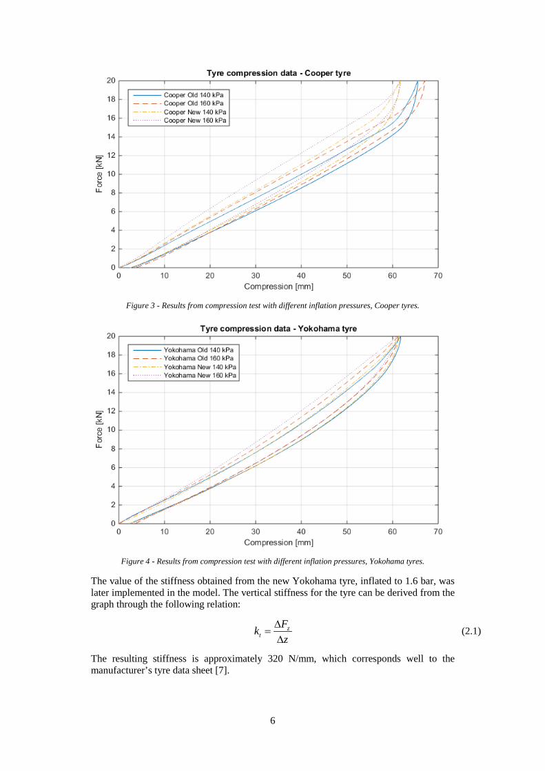
The tire patch of both types was slightly wider than the pressure plates that were used in the test. During the end of the compression cycle, the Cooper tyre carcass yielded somewhat and started to fold on top of the pressure plate. The results can be seen in Figure 3. The resulting vertical stiffness’ for the Yokohama tyres are shown in Figure 4.
6
Figure 3 - Results from compression test with different inflation pressures, Cooper tyres.
Figure 4 - Results from compression test with different inflation pressures, Yokohama tyres.
The value of the stiffness obtained from the new Yokohama tyre, inflated to 1.6 bar, was later implemented in the model. The vertical stiffness for the tyre can be derived from the graph through the following relation:
zt
Fkz
∆=
∆ (2.1)
The resulting stiffness is approximately 320 N/mm, which corresponds well to the manufacturer’s tyre data sheet [7].
7
3 Software introduction
Included in this chapter is an introduction to the four simulation software investigated.
3.1 CarSim
The software version used was CarSim 8.2.2.
CarSim is based on the VehicleSim platform developed by Mechanical Simulation Corporation and the software is a simulation tool for analysing vehicle dynamics. The simulation model has 15 degrees of freedom and the equations are based on rigid body motions. The math models acquires the required data from text based files called parsfiles. Each driving event, sub-model, component etc. can be described by the parsfiles which are accessible to the user for modification purposes. The software includes a driver control with open and closed loop steering, braking and acceleration. It gives the possibility to set up different driving events with high complexity [8].
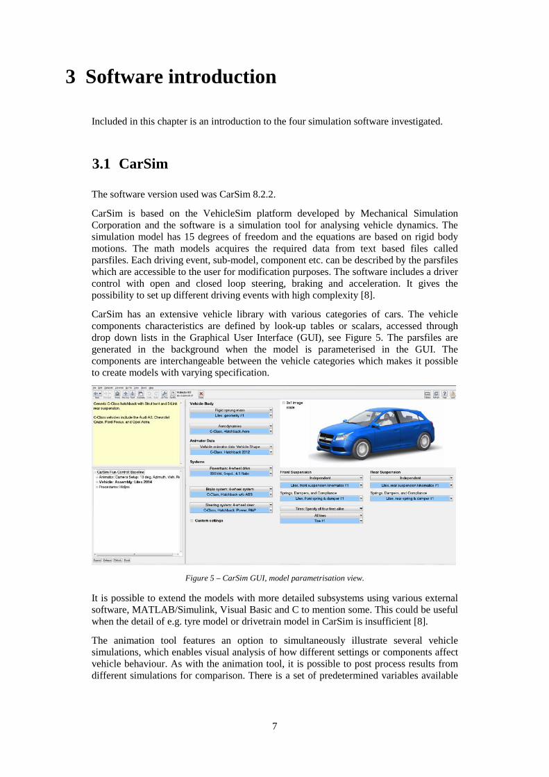
CarSim has an extensive vehicle library with various categories of cars. The vehicle components characteristics are defined by look-up tables or scalars, accessed through drop down lists in the Graphical User Interface (GUI), see Figure 5. The parsfiles are generated in the background when the model is parameterised in the GUI. The components are interchangeable between the vehicle categories which makes it possible to create models with varying specification.
Figure 5 – CarSim GUI, model parametrisation view.
It is possible to extend the models with more detailed subsystems using various external software, MATLAB/Simulink, Visual Basic and C to mention some. This could be useful when the detail of e.g. tyre model or drivetrain model in CarSim is insufficient [8].
The animation tool features an option to simultaneously illustrate several vehicle simulations, which enables visual analysis of how different settings or components affect vehicle behaviour. As with the animation tool, it is possible to post process results from different simulations for comparison. There is a set of predetermined variables available
8
that can form the axes in the plot window. Modifying the parsfiles, it is most likely possible to calculate energy absorption in the suspension and other useful quantities. Furthermore, CarSim has a tool for defining 3D road profiles which can be directly implemented from Excel sheets.
3.2 ADAMS/Car
The software version used was ADAMS/Car 2013.
Adams/Car is a multibody dynamic simulation tool used to analyse the dynamic behaviour of a vehicle or its subsystems. The multibody dynamic system consists of links or solid bodies interconnected by joints and bushings. Forces are applied to the system and the movement of parts are calculated by the software [9].
A simulation model is created in several steps, a short description will follow. First, a template has to be made where hard points are defined. A part is then created with the key points and, optionally, a geometry is set to the part. Each part has individual properties which are defined either by assigning a material property to the geometry or, if the values are known, simply enter them in the parts property window. Attachments between the parts has to be created. The attachments can be of joint or bushing type. A sub system can then be generated with the defined parts. Communicators has to be assigned appropriately to each sub system to create a functioning model assembly. The communicators enables information exchange between the sub systems. The sub systems have a set of input and output communicators which has to be assigned correctly. A set of sub systems can then be put together into an assembly which then can be analysed [10].
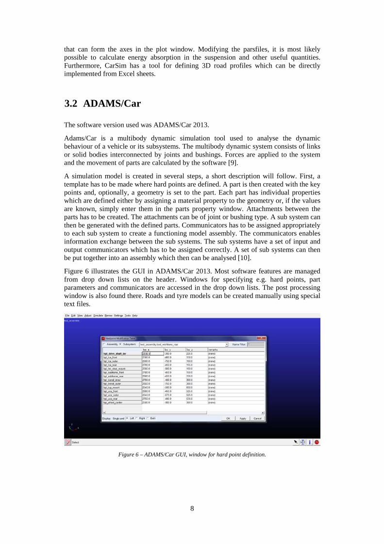
Figure 6 illustrates the GUI in ADAMS/Car 2013. Most software features are managed from drop down lists on the header. Windows for specifying e.g. hard points, part parameters and communicators are accessed in the drop down lists. The post processing window is also found there. Roads and tyre models can be created manually using special text files.
Figure 6 – ADAMS/Car GUI, window for hard point definition.
9
3.3 LMS Amesim
The software version used was LMS Amesim rev 13 ST, run on a trial license.
LMS Amesim is a multi-domain system simulation platform which means that it is possible to simulate systems in a variety of physical domains, on their own or combined. The existing libraries of components range from the mechanical domain to the hydraulic, thermal, electrical and pneumatic domain, among others.
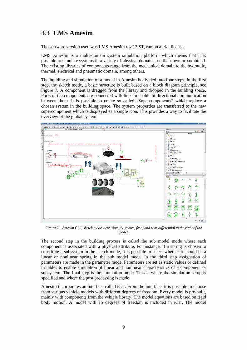
The building and simulation of a model in Amesim is divided into four steps. In the first step, the sketch mode, a basic structure is built based on a block diagram principle, see Figure 7. A component is dragged from the library and dropped in the building space. Ports of the components are connected with lines to enable bi-directional communication between them. It is possible to create so called “Supercomponents” which replace a chosen system in the building space. The system properties are transferred to the new supercomponent which is displayed as a single icon. This provides a way to facilitate the overview of the global system.
Figure 7 – Amesim GUI, sketch mode view. Note the centre, front and rear differential to the right of the
model.
The second step in the building process is called the sub model mode where each component is associated with a physical attribute. For instance, if a spring is chosen to constitute a subsystem in the sketch mode, it is possible to select whether it should be a linear or nonlinear spring in the sub model mode. In the third step assignation of parameters are made in the parameter mode. Parameters are set as static values or defined in tables to enable simulation of linear and nonlinear characteristics of a component or subsystem. The final step is the simulation mode. This is where the simulation setup is specified and where the post processing is made.
Amesim incorporates an interface called iCar. From the interface, it is possible to choose from various vehicle models with different degrees of freedom. Every model is pre-built, mainly with components from the vehicle library. The model equations are based on rigid body motion. A model with 15 degrees of freedom is included in iCar. The model
10
consists of seven supercomponents; chassis, suspension, tires, road, aerodynamics, steering, driver controls. The model is completed with brake – and differential components. The driving torque input to the differential is managed by a velocity control module, replacing an engine supercomponent.
It is possible to install an application which helps the user to generate tables for suspension kinematics without hard point data. If a set of static values are known, the axle properties can be calculated and tables are created based on the entered values.
When switching to simulation mode, graphs can be created by point and drag the component of interest to the post processing window, which has replaced the model library space on the right hand side, see Figure 7. Road profiles can be constructed using a different set of tables.
3.4 MATLAB
The software version used was MATLAB 2014b.
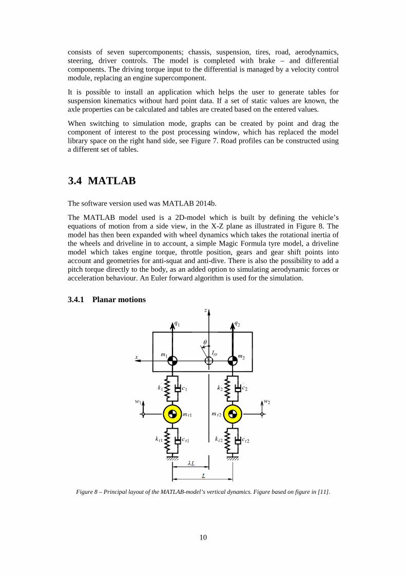
The MATLAB model used is a 2D-model which is built by defining the vehicle’s equations of motion from a side view, in the X-Z plane as illustrated in Figure 8. The model has then been expanded with wheel dynamics which takes the rotational inertia of the wheels and driveline in to account, a simple Magic Formula tyre model, a driveline model which takes engine torque, throttle position, gears and gear shift points into account and geometries for anti-squat and anti-dive. There is also the possibility to add a pitch torque directly to the body, as an added option to simulating aerodynamic forces or acceleration behaviour. An Euler forward algorithm is used for the simulation.
3.4.1 Planar motions
Figure 8 – Principal layout of the MATLAB-model’s vertical dynamics. Figure based on figure in [11].

11
Equations (3.1) through (3.5) defines the planar motion of the vehicle in a simplified case with no anti-features active, linear springs, dampers and tyres, and no longitudinal motion of the suspension.
,1 ,2z z zF F F mg= + − (3.1)
,1 ,2x x xF F F= + (3.2)
,2 ,1(1 )yy z z xI F L F L F Lθ λ λ κ= − − + (3.3)
where
, , ,( ) ( )z i i t i i i t i iF k z z c z z= − + − (3.4)
and
, , , , ,( ) ( )zt i t i i t i t i i t iF k w z c w z= − + − (3.5)
give the vertical forces from the tyres and the suspension, and index i indicates front and rear. The longitudinal forces Fx comes from the tyre model, which is explained in the following section.
3.4.2 Longitudinal tyre model A simple version of the Pajceka Magic Formula tyre model [12] is used to generate longitudinal forces. It does therefore not use any physical properties of the tyre, but is only slip curve based. This means that the wheels have to be slipping against the road surface before any tractive force is created. Wheel slip is calculated using the definition in equation (3.6) where ω is the rotational speed of the wheel, vx the vehicle velocity in the x-direction and rr the radius of the wheel.
x
r
vr
ωκ
ω
− = (3.6)
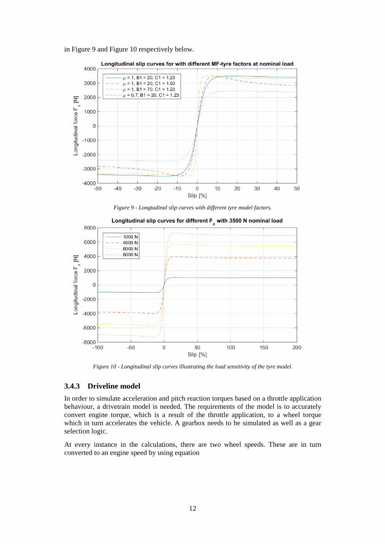
This simplified Magic Formula model only uses seven parameters to calculate the generated tyre force, which is enough to illustrate the principle behaviour of a tyre in the longitudinal direction, but not more than easily manageable for a user when trying to quickly replicate with decent accuracy. The equation for longitudinal tyre force Fx is given in (3.7),
,(1 ( ))sin(Catan(B ))xi zi zi z nomF F D F Fm κ= − − (3.7)
where μ is a peak-friction value (typical range from 0.1 for ice to 1.5 for racing slicks on tarmac), B is a stiffness factor (typical range 10-40) which affects the longitudinal stiffness of the tyre. C is a crest factor (typical range 1-1.4), which adjust the location and severity of the tyre force peak. D is a load-sensitivity factor (typical size 10-5) which aid to replicate the load sensitivity of a tyre as is usually has higher friction utilisation at low load relative to its nominal load and low friction utilisation at high load relative to its nominal load. A figure illustrating four slip curves for four different configurations of μ, B, and C as well as a figure illustrating the load sensitivity of the slip curves can be seen
12
in Figure 9 and Figure 10 respectively below.
Figure 9 - Longtudinal slip curves with different tyre model factors.
Figure 10 - Longitudinal slip curves illustrating the load sensitivity of the tyre model.
3.4.3 Driveline model In order to simulate acceleration and pitch reaction torques based on a throttle application behaviour, a drivetrain model is needed. The requirements of the model is to accurately convert engine torque, which is a result of the throttle application, to a wheel torque which in turn accelerates the vehicle. A gearbox needs to be simulated as well as a gear selection logic.
At every instance in the calculations, there are two wheel speeds. These are in turn converted to an engine speed by using equation

13
1 2 =2D
ω ωω + (3.8)
which is considered to be the rotational speed of the driveline after the final drive. This is converted to a set of engine speeds by using equation
= E D i fU Uω ω ⋅ ⋅ (3.9)
where Ui denotes all of the possible gears. A routine to pick the lowest gear possible without exceeding the maximum engine rotational speed allowed is then run, in order to maximise acceleration. The engine speed is then used together with a look-up table and the throttle position to find the correct driving torque. If the current engine speed exceeds the maximum rotational speed allowed, a simple engine speed limiter is introduced which applies a small amount of engine braking. Two simplifications that are made are that the engine always hits its speed limiter before shifting up and the gear selection logic never shifts gear when the car is in the air, to simulate real jumping behaviour.
The driving engine torque is converted to a driveline torque by using Equation (3.10)
= D E i fT T U U⋅ ⋅ (3.10)
The torque is split between the axles by a torque split factor which is given as a car parameter and then put on to the driving wheels. The net torque of the wheel is then calculated and translated into a net acceleration of the wheel. This net torque is also applied to the body in the opposite direction to simulate the resulting torque on the body. As the engines in most cases are longitudinally mounted, the engine itself does not affect the car’s rotation in a planar view.
i, ,inet i x rT T F r= − ⋅ (3.11)
,ii x ri
w
T F rJ
ω− ⋅
= (3.12)
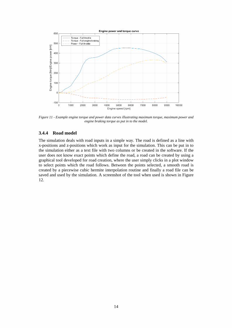
The engine torque TE is interpolated from a torque curve which is given by the user as a set of input parameters. The engine model also facilitates engine braking. As a simple estimate of the engine braking torque, the engine torque curve at full throttle is multiplied by a chosen factor and negated, to create the engine braking torque curve. This is done to be able to simulate the effect of a braking engine torque when jumping. A typical set of engine input parameters are given in Figure 11.
14
Figure 11 - Example engine torque and power data curves illustrating maximum torque, maximum power and
engine braking torque as put in to the model.
3.4.4 Road model The simulation deals with road inputs in a simple way. The road is defined as a line with x-positions and z-positions which work as input for the simulation. This can be put in to the simulation either as a text file with two columns or be created in the software. If the user does not know exact points which define the road, a road can be created by using a graphical tool developed for road creation, where the user simply clicks in a plot window to select points which the road follows. Between the points selected, a smooth road is created by a piecewise cubic hermite interpolation routine and finally a road file can be saved and used by the simulation. A screenshot of the tool when used is shown in Figure 12.

15
Figure 12 - Screenshot of the graphical road creation tool created for the MATLAB-simulation model
3.4.5 Driver inputs To simulate driver inputs there are a few different ways available for the user of this simulation software. There are four ways of defining driver behaviour; coasting, full throttle/brake, cruise control and by using a throttle trace.
The coasting is simulated by setting the vehicle to an initial speed and then letting the vehicle coast along the road without any torque inputs into the driveline. As the simulation does not consider rolling resistance nor aerodynamic drag, this can be useful when investigating how the vehicle slows down or speeds up over undulation.
Full throttle mode simulates the car driving with the throttle wide open. This is useful to simulate full throttle starts or acceleration events. Full braking mode lets the car roll with an initial speed for a predetermined distance. When the vehicle reaches that set distance, the driveline produces a negative driving torque, which matches the maximum braking force the tyres can manage, before easing off the negative torque as the vehicle comes to a standstill.
There is also a cruise control implemented into the model. By setting a speed, the car will attempt to follow that speed by applying the required torque to the driveline. In this mode, the car is not limited to the ability of the engine, which means that the vehicle will have infinite power to follow the desired speed. This is useful when trying to simulate jumping off a jump at a given speed, for example when comparing with measured data.
The fourth option is using a throttle trace which is given as a text file of two columns of throttle position and time or distance. This allows for simulating a jump complete with real or manufactured driver data.
16
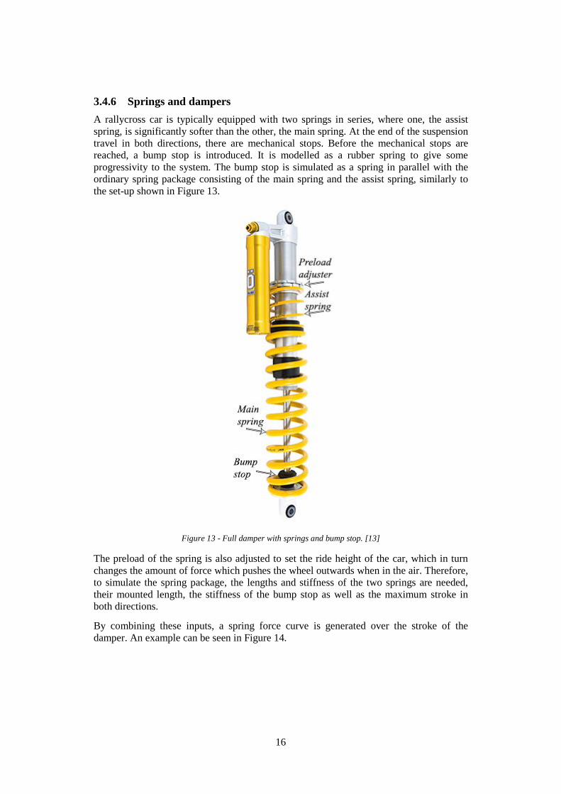
3.4.6 Springs and dampers A rallycross car is typically equipped with two springs in series, where one, the assist spring, is significantly softer than the other, the main spring. At the end of the suspension travel in both directions, there are mechanical stops. Before the mechanical stops are reached, a bump stop is introduced. It is modelled as a rubber spring to give some progressivity to the system. The bump stop is simulated as a spring in parallel with the ordinary spring package consisting of the main spring and the assist spring, similarly to the set-up shown in Figure 13.
Figure 13 - Full damper with springs and bump stop. [13]
The preload of the spring is also adjusted to set the ride height of the car, which in turn changes the amount of force which pushes the wheel outwards when in the air. Therefore, to simulate the spring package, the lengths and stiffness of the two springs are needed, their mounted length, the stiffness of the bump stop as well as the maximum stroke in both directions.
By combining these inputs, a spring force curve is generated over the stroke of the damper. An example can be seen in Figure 14.

17
Figure 14 – Spring force and spring stroke. The figure displays hysteresis in the bump stop or drop stop
towards the end of the stroke where the blue line illustrates a positive stroke velocity and the red line illustrates a negative stroke velocity.
The dampers are modelled as shown in Figure 15 based on force-velocity curves which are placed in a look-up table. This data is acquired from damper dynamometer testing where the damper is exerted to a given set of velocities and the resulting force is measured.
Figure 15 - Flowchart of damper model in MATLAB model.
A typical example of a damper force-velocity curve is shown in Figure 16.
Figure 16 - Example force-velocity curve showing the damper force in compression and rebound stroke.

18
The damper modelling in this simulation has the option of being reactive to other types of inputs than just damper displacement rate, which in turns allows the model to be applied for investigating damper characteristics which do not respond to displacement rate, cannot be replicated in reality or which are yet not produced.
In the model there are also longitudinal springs, longitudinal dampers, anti-squat and anti-dive represented. The longitudinal springs and dampers keep the wheels in place in longitudinal directions and are modelled in a similar fashion to the vertical suspension. For the purpose of this study the longitudinal springs have been made much stiffer than the vertical springs and can be considered stiff. Anti-features have been added and are used during this study, however the effect on jumping performance has been found negligible.
3.4.7 GUI A GUI was developed to increase the user friendliness of the simulation tool. Figure 17 illustrates the main window where the simulation is set up. In this window the user can specify the driving scenario, road profile and throttle application. The animation panel is viewable and the post processing tools can also be seen here. The vehicle parameterisation window and road creation, described in 3.4.4 are also accessible from the main window.
Figure 17 - The main window view of the created MATLAB GUI.
The vehicle is configured in a car parameter window. The vehicle parameters which have constant values are specified in boxes while motion ratio, damper curves and other non-linear variables are entered in tables. Tag-lines appears over boxes to give a description of the quantity to be entered. Damper curves can be read into the software from Excel sheets which are produced by Öhlins’ shock absorber dynamometer software. Several fully configured vehicles have been made and exist in the software to provide a set of baselines
19
to run simulations from.
Each simulation run is saved and is accessible in the post-processing section. The user has the possibility to compare the simulated models with different vehicle parameters, throttle application or driven roads.
3.4.8 MATLAB summary The MATLAB simulation is based on a half-car model which has been adapted for jumping use with vertical and longitudinal tyre models, a driveline model, road model with road creation module and a driver input model. Spring, dampers and bump stops are modelled with look-up tables, taking different preloads, ride heights, spring stiffness, spring combinations and hysteresis of rubber components into account. All of the input data in to the model is parameter based and not based on kinematic relationships, in similar fashion to Amesim and CarSim.
To initiate a vehicle simulation, the software is parameterised with the vehicle parameters, a road profile chosen or created and a driver mode chosen. The vehicle is then simulated along the chosen road profile and the chosen results are presented as graphic plots from the GUI.

20
21
4 Simulation model setup
This chapter presents how the models were built in the different software, the vehicle properties that were used to parameterise the models and specifies which initial velocities and road profiles that were implemented before the validation.
4.1 Vehicle properties
The vehicle properties assigned to the models corresponded to the setup that the reference car had during the tests on track A and B, see section 2.3. The vehicle settings and data can be seen in Appendix A.
4.2 Road profile creation
Road profiles were created in each software based on the measured data from circuit A and B. The initial speed on jump B was 28.6 m/s while the initial speed on jump A1 and jump A2 was 25 m/s and 30.6 m/s respectively. The road profiles can be seen in Figure 1. The friction coefficient was assumed to be 0.85. The throttle was assumed to be fully applied through the simulation sequence.
4.3 CarSim
A C-class vehicle was chosen as the base model. The geometry, suspension kinematics, tires, springs and dampers were altered so that it corresponded to the reference vehicle. The values that could not be obtained from the reference car but had to be entered in the software were approximated. The aerodynamic properties was kept as default while the drivetrain parameters were set to a 250 kW engine with four wheel drive and limited slip differentials front and rear.
Road profiles were created using Road: 3D surface. The centreline geometry: Horizontal (X-Y) table were set to: straight, while the vertical and longitudinal measured data points were implemented in Centreline elevation: Z vs S, creating the different 3D roads.
4.4 ADAMS/Car
The model was created using templates from ADAMS/Car shared library. At this point in time, no hard points for the reference car could be been obtained. Double wishbone templates for front and rear were modified so that the wheelbase, track width and motion ratio corresponded to the reference car. A rack and pinion steering sub system was included in the vehicle assembly. The driveline was however excluded due to lack of data. The rest of the model could be parameterised with the reference car data.
22
A road was created from the measured track data acquired from the GPS. The measured points in the vertical and longitudinal direction were implemented in a .rtf –file as rows and then fitted with linear interpolation. A Straight-line/Maintain –event was simulated with the initial velocities mentioned in section 4.2.
The validation of the ADAMS/Car model was excluded. This is due to that even at an early stage, the amount of time which was consumed by setting up an ADAMS/Car model was many times higher than time needed for any of the other models. Therefore it was concluded that ADAMS/Car was not a viable option for the end purpose of this thesis and ADAMS/Car was therefore excluded for the rest of this study.
4.5 LMS Amesim
The 15 degree of freedom vehicle model from the iCar interface was chosen to represent the reference car. The model was based on a tutorial templates and differentials were added to simulate a four wheel drive system, see Figure 7. The model was parameterised using the reference car data. The values that could not be obtained from the reference car but had to be entered in the software were approximated.
The road profiles were created using 3D tables.
4.6 MATLAB
The model of the rallycross car was parameterised using real and measured values for masses, dimensions, spring stiffness, damper curves, anti-features, engine power, tyre stiffness, bump stops and motion ratios, seen in Appendix A. Road profiles were used from measured jumps.

23
5 Evaluation of models
The models were validated against the logged data acquired from testing with the reference car running on track A and B, see section 2.3. The quantities compared during the validation were wheel displacement and wheel displacement rate and time of impact for the front and rear axle respectively. The time of impact and the time difference between front and rear axle indicates the pitch behaviour of the reference car and the simulation models.
The models were also compared to each other with respect to the criteria set up by Öhlins, presented in section 1.4. The aim of this part of the project was to decide upon the most suitable software for continuous work with the master thesis project, again with the respect to criteria set up.
5.1 Validation
ADAMS/Car was excluded from the validation as explained in section 4.4.
The reference car had run on all of the jumps which were measured as mentioned in section 2.3. All of the simulation software were setup to replicate the behaviour of the vehicle as accurately as possible. However, there were, as previously mentioned, situations where the software itself was a limiting factor when it came to predict the desired behaviour, described in section 3. Examples of this are software not being able to describe non-linear tyres.
For all three jumps (A1, A2 and B) front and rear wheel displacement and displacement rate is studied, as well an indication of pitch rotation, whether the front or the rear wheel touches the ground first.
Both left and right wheel displacement and displacement rate are shown from the reference car to give an indication of how the vehicle landed for these jumps. All measurements shown are indicative of a typical behaviour for this car on the respective jump with the current driver.
The results from the validation for jump A1 and jump B will be analysed below. As jump A2 does not add anything to the analysis, its results are shown in Appendix B.
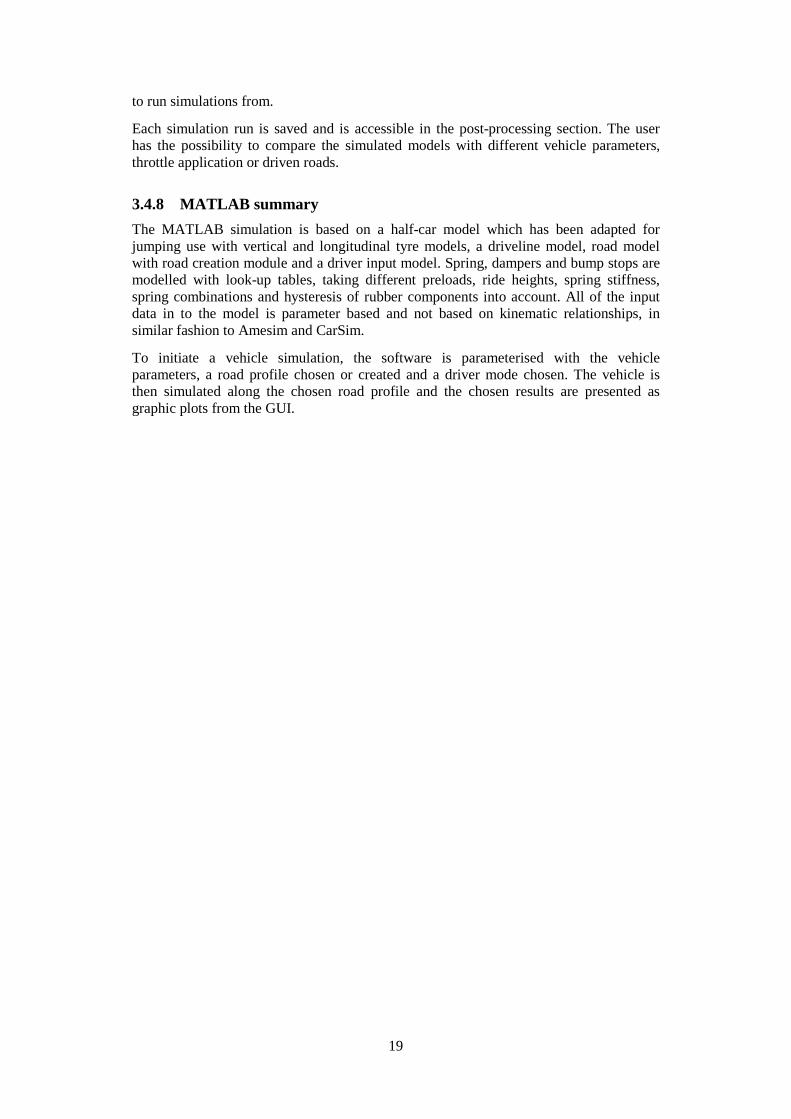
5.1.1 Jump A1 The front wheel displacement of jump A1 is shown in Figure 18, where it can be seen that the left-hand front wheel of the reference car has a much larger displacement than the right-hand front wheel or any of the simulation models. This indicates that the vehicle lands with a quite large roll angle, which skews the results, not only as more energy is absorbed by the first wheel to hit the ground but also as translational energy is put into rotational motion. However, it is clear that all of the simulations match the front right wheel quite accurately.
24
Figure 18 - Front wheel displacements for jump A1.
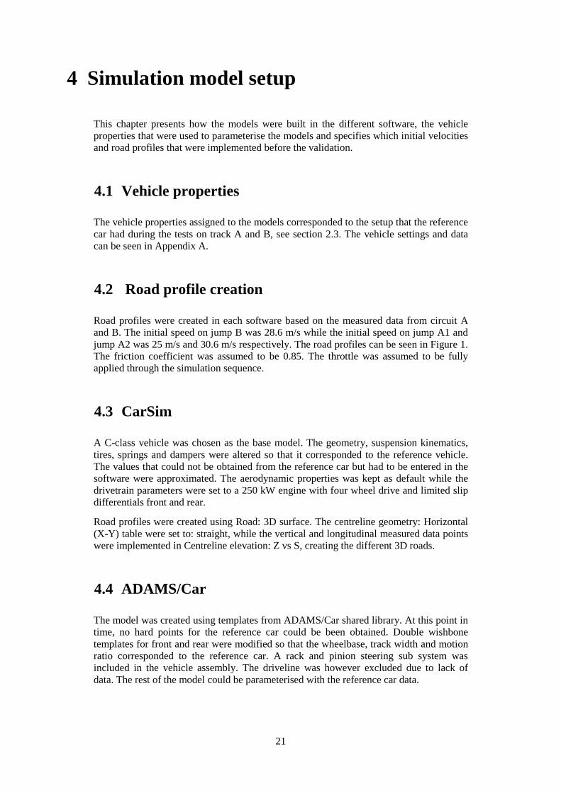
As can be shown by the front wheel displacement rate in Figure 19, the MATLAB and CarSim models match the front wheel speed quite well. Amesim underestimates the displacement rate to some extent. Again, the left front wheel, which makes contact with the ground later due to landing with a large roll angle, has to absorb energy from the translation of the vehicle vertically as well as the rotation of the vehicle in roll, giving a higher displacement rate.
Figure 19 - Front wheel displacement rates for jump A1.
It can also be seen in Figure 20 that all software manage to replicate the rear wheel displacement rather well. Note that the rear right suspension sensor was broken during the test on track A and that therefore no rear right wheel displacement data from that test is shown. The used wheel stroke and peak wheel velocities is shown in Table 1 below.

25
Figure 20 - Rear wheel displacement for jump A1.
Studying the rear wheel displacement rate in Figure 21 suggests that the pattern from the front wheel displacement rate occurs here as well. The MATLAB and CarSim simulations overestimated the real damper speed slightly, probably due to a larger vehicle pitch motion, indicated by the time difference between front and rear axle ground contact. The time difference is quite large compared to Amesim. Amesim slightly underestimates the rear wheel displacement speed.
Figure 21 - Rear wheel displacement rate for jump A1. The rear right wheel speed is not plotted due to faulty
sensor.
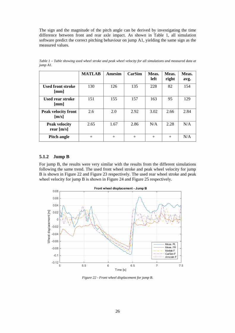
26
The sign and the magnitude of the pitch angle can be derived by investigating the time difference between front and rear axle impact. As shown in Table 1, all simulation software predict the correct pitching behaviour on jump A1, yielding the same sign as the measured values.
Table 1 – Table showing used wheel stroke and peak wheel velocity for all simulations and measured data at jump A1.
MATLAB Amesim CarSim Meas. left
Meas. right
Meas. avg.
Used front stroke [mm]
130 126 135 228 82 154
Used rear stroke [mm]
151 155 157 163 95 129
Peak velocity front [m/s]
2.6 2.0 2.92 3.02 2.66 2.84
Peak velocity rear [m/s]
2.65 1.67 2.86 N/A 2.28 N/A
Pitch angle + + + + + N/A
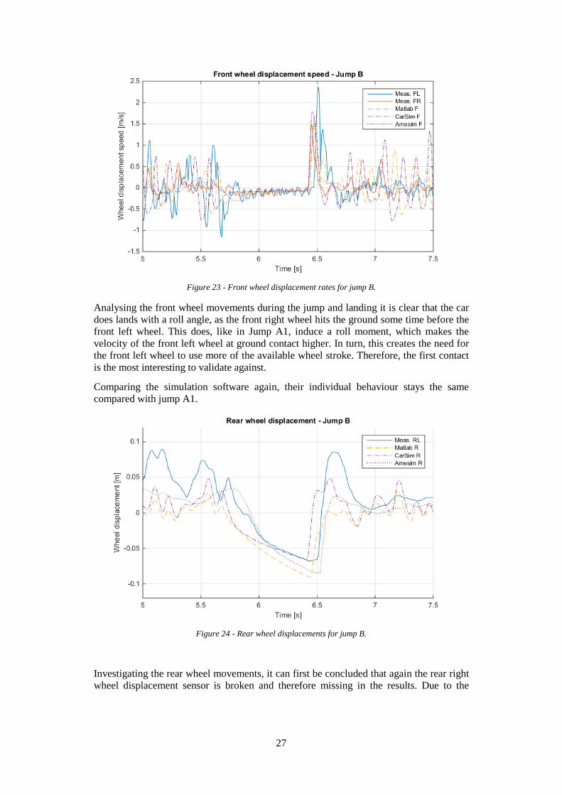
5.1.2 Jump B For jump B, the results were very similar with the results from the different simulations following the same trend. The used front wheel stroke and peak wheel velocity for jump B is shown in Figure 22 and Figure 23 respectively. The used rear wheel stroke and peak wheel velocity for jump B is shown in Figure 24 and Figure 25 respectively.
Figure 22 - Front wheel displacement for jump B.
27
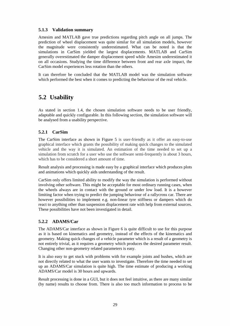
Figure 23 - Front wheel displacement rates for jump B.
Analysing the front wheel movements during the jump and landing it is clear that the car does lands with a roll angle, as the front right wheel hits the ground some time before the front left wheel. This does, like in Jump A1, induce a roll moment, which makes the velocity of the front left wheel at ground contact higher. In turn, this creates the need for the front left wheel to use more of the available wheel stroke. Therefore, the first contact is the most interesting to validate against.
Comparing the simulation software again, their individual behaviour stays the same compared with jump A1.
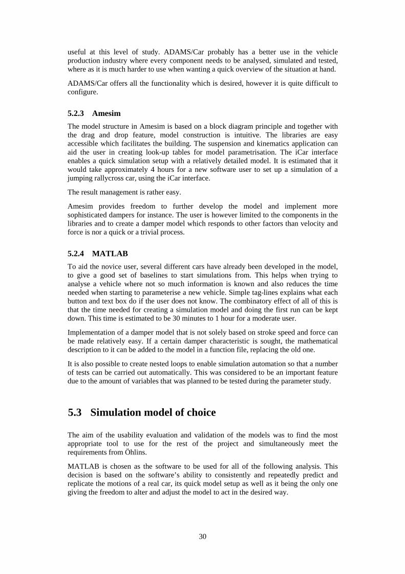
Figure 24 - Rear wheel displacements for jump B.
Investigating the rear wheel movements, it can first be concluded that again the rear right wheel displacement sensor is broken and therefore missing in the results. Due to the

28
difference between the measured data for the front wheels it can be assumed that the jump performed with a large roll angle which, as previously explained, can induce high utilisation of available stroke and high displacement rates. Therefore it is difficult to make a straight comparison between the measured data and the simulation data.
When comparing the software to each other it is clear that all software underestimates the utilised wheel stroke but CarSim is closest to the measured values. CarSim and MATLAB slightly overestimates the rear wheel displacement speed and Amesim underestimates it with approximately the same amount.
Figure 25 - Rear wheel displacement rate for jump B.
MATLAB and Amesim managed to predict the landing pitch angle, which is shown in Table 2. CarSim predicted a negative pitch angle, when the reference car landed with the front axle first.
Table 2 - Table showing used wheel stroke and peak wheel velocity for all simulations and measured data at jump B.
MATLAB Amesim CarSim Meas. left
Meas. right
Meas. avg.
Used front stroke [mm]
104 87 113 161 65 113
Used rear stroke [mm]
98 86 97 150 N/A N/A
Peak velocity front [m/s]
1.51 1.65 1.79 2.37 1.50 1.93
Peak velocity rear [m/s]
1.65 1.13 1.84 1.37 N/A N/A
Pitch angle + + - + N/A N/A
29
5.1.3 Validation summary Amesim and MATLAB gave true predictions regarding pitch angle on all jumps. The prediction of wheel displacement was quite similar for all simulation models, however the magnitude were consistently underestimated. What can be noted is that the simulations in CarSim yielded the largest displacements. MATLAB and CarSim generally overestimated the damper displacement speed while Amesim underestimated it on all occasions. Studying the time difference between front and rear axle impact, the CarSim model experiences less rotation than the others.
It can therefore be concluded that the MATLAB model was the simulation software which performed the best when it comes to predicting the behaviour of the real vehicle.
5.2 Usability
As stated in section 1.4, the chosen simulation software needs to be user friendly, adaptable and quickly configurable. In this following section, the simulation software will be analysed from a usability perspective.
5.2.1 CarSim The CarSim interface as shown in Figure 5 is user-friendly as it offer an easy-to-use graphical interface which grants the possibility of making quick changes to the simulated vehicle and the way it is simulated. An estimation of the time needed to set up a simulation from scratch for a user who use the software semi-frequently is about 3 hours, which has to be considered a short amount of time.
Result analysis and processing is made easy by a graphical interface which produces plots and animations which quickly aids understanding of the result.
CarSim only offers limited ability to modify the way the simulation is performed without involving other software. This might be acceptable for most ordinary running cases, when the wheels always are in contact with the ground or under low load. It is a however limiting factor when trying to predict the jumping behaviour of a rallycross car. There are however possibilities to implement e.g. non-linear tyre stiffness or dampers which do react to anything other than suspension displacement rate with help from external sources. These possibilities have not been investigated in detail.
5.2.2 ADAMS/Car The ADAMS/Car interface as shown in Figure 6 is quite difficult to use for this purpose as it is based on kinematics and geometry, instead of the effects of the kinematics and geometry. Making quick changes of a vehicle parameter which is a result of a geometry is not entirely trivial, as it requires a geometry which produces the desired parameter result. Changing other non-geometry related parameters is easy.
It is also easy to get stuck with problems with for example joints and bushes, which are not directly related to what the user wants to investigate. Therefore the time needed to set up an ADAMS/Car simulation is quite high. The time estimate of producing a working ADAMS/Car model is 30 hours and upwards.
Result processing is done in a GUI, but it does not feel intuitive, as there are many similar (by name) results to choose from. There is also too much information to process to be
30
useful at this level of study. ADAMS/Car probably has a better use in the vehicle production industry where every component needs to be analysed, simulated and tested, where as it is much harder to use when wanting a quick overview of the situation at hand.
ADAMS/Car offers all the functionality which is desired, however it is quite difficult to configure.
5.2.3 Amesim The model structure in Amesim is based on a block diagram principle and together with the drag and drop feature, model construction is intuitive. The libraries are easy accessible which facilitates the building. The suspension and kinematics application can aid the user in creating look-up tables for model parametrisation. The iCar interface enables a quick simulation setup with a relatively detailed model. It is estimated that it would take approximately 4 hours for a new software user to set up a simulation of a jumping rallycross car, using the iCar interface.
The result management is rather easy.
Amesim provides freedom to further develop the model and implement more sophisticated dampers for instance. The user is however limited to the components in the libraries and to create a damper model which responds to other factors than velocity and force is nor a quick or a trivial process.
5.2.4 MATLAB To aid the novice user, several different cars have already been developed in the model, to give a good set of baselines to start simulations from. This helps when trying to analyse a vehicle where not so much information is known and also reduces the time needed when starting to parameterise a new vehicle. Simple tag-lines explains what each button and text box do if the user does not know. The combinatory effect of all of this is that the time needed for creating a simulation model and doing the first run can be kept down. This time is estimated to be 30 minutes to 1 hour for a moderate user.
Implementation of a damper model that is not solely based on stroke speed and force can be made relatively easy. If a certain damper characteristic is sought, the mathematical description to it can be added to the model in a function file, replacing the old one.
It is also possible to create nested loops to enable simulation automation so that a number of tests can be carried out automatically. This was considered to be an important feature due to the amount of variables that was planned to be tested during the parameter study.
5.3 Simulation model of choice
The aim of the usability evaluation and validation of the models was to find the most appropriate tool to use for the rest of the project and simultaneously meet the requirements from Öhlins.
MATLAB is chosen as the software to be used for all of the following analysis. This decision is based on the software’s ability to consistently and repeatedly predict and replicate the motions of a real car, its quick model setup as well as it being the only one giving the freedom to alter and adjust the model to act in the desired way.
31
6 Parameter study
A parameter study was conducted with the MATLAB simulation model to analyse the impact various parameters have on the vehicle motion during the jumping phase. Seven variables were tested separately on three different levels; jump entry speed, throttle application, front and rear spring stiffness, front and rear damper stiffness and the longitudinal position of centre of gravity. The model was exerted to four different jumps. A total of 243 combinations of vehicle settings were tested under 36 different driving conditions. The total amount of simulation runs were 8748. In addition to this study, some analyses were done which was directed to driver behaviour only.
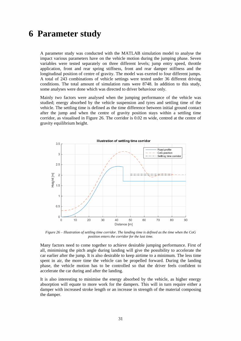
Mainly two factors were analysed when the jumping performance of the vehicle was studied; energy absorbed by the vehicle suspension and tyres and settling time of the vehicle. The settling time is defined as the time difference between initial ground contact after the jump and when the centre of gravity position stays within a settling time corridor, as visualised in Figure 26. The corridor is 0.02 m wide, centred at the centre of gravity equilibrium height.
Figure 26 – Illustration of settling time corridor. The landing time is defined as the time when the CoG
position enters the corridor for the last time.
Many factors need to come together to achieve desirable jumping performance. First of all, minimising the pitch angle during landing will give the possibility to accelerate the car earlier after the jump. It is also desirable to keep airtime to a minimum. The less time spent in air, the more time the vehicle can be propelled forward. During the landing phase, the vehicle motion has to be controlled so that the driver feels confident to accelerate the car during and after the landing.
It is also interesting to minimise the energy absorbed by the vehicle, as higher energy absorption will equate to more work for the dampers. This will in turn require either a damper with increased stroke length or an increase in strength of the material composing the damper.

32
All of the car control factors such as airtime and pitch angle, with exception of settling time, can be related to the energy absorbed by the vehicle. A minimisation of energy absorption equates to a shorter airtime and a lower pitch rate while the vehicle is airborne. This is due to that a longer airtime generally means that the vehicle has reached a higher altitude during the jumping phase. A higher altitude will increase the potential energy of the body, hence a larger amount of energy absorption is required when it lands. The same goes for pitch angle. A larger pitch angle during landing will require larger energy absorption since when ground contact occurs by either axle, a pitch acceleration is initiated due to the vertical force that acts through the suspension, on the body. More energy will be used for rotation, which later will be damped out from the system.
The energy absorbed is calculated by integrating the power which is needed to deflect the suspension and the tyres, as shown in equation (6.1).
( ) ( )( )/
11
t dt
iE Fdx F x i x i
=
= = − −∑∫ (6.1)
6.1 Simulation setup
The three previously measured road sections, A1, A2 and B were used during the parameter study and a road section C was added. This profile was created given the comments from interviewees regarding the shape of problematic jumps, see section 2.1. The road profiles are illustrated in Figure 27.
Figure 27 – Road profiles used in the simulation for the parameter study.
The profiles were cut off to ensure that the vehicle always would land on a flat surface. This facilitated the result analysis and it was possible to compare the different levels of energy absorption and settling time equally between the simulation runs. The road sections are automatically extrapolated until the end of the simulation.

33
The investigated parameters related to the vehicle were; longitudinal position of the centre of gravity, spring stiffness and damper stiffness for front and rear axle respectively. The parameters were tested on three different levels, see Table 3.
Table 3 – Test parameters.
Variable Front spring
Rear spring
Front damper
Rear damper λ
Level 1/2/3 1/2/3 1/2/3 1/2/3 Front/Mid/Rear
Level 1 indicates that a lower spring or damper stiffness is tested, while level 2 is assigned as the actual stiffness of spring or damper of the real car, see Appendix A. Level 3 is a stiffer setting.
Three different driving behaviour and three different jump entry speeds were tested. The velocities are specified in Table 4 while the throttle applications are shown in Table 4.
Table 4 – The initial speed for each jump and a subsequent speed increase of 5 km/h per run.
Jump A1 A2 B C
Entry speed [km/h] 50/55/60 95/100/105 77/82/87 31/36/41
The throttle application was modelled as a function of distance. In the case of throttle lift off, a negative motor torque is applied to the wheels as explained in 3.4.3.
Figure 28 – Simulating different driving behaviour by running the model with different throttle applications.
34
6.2 Results
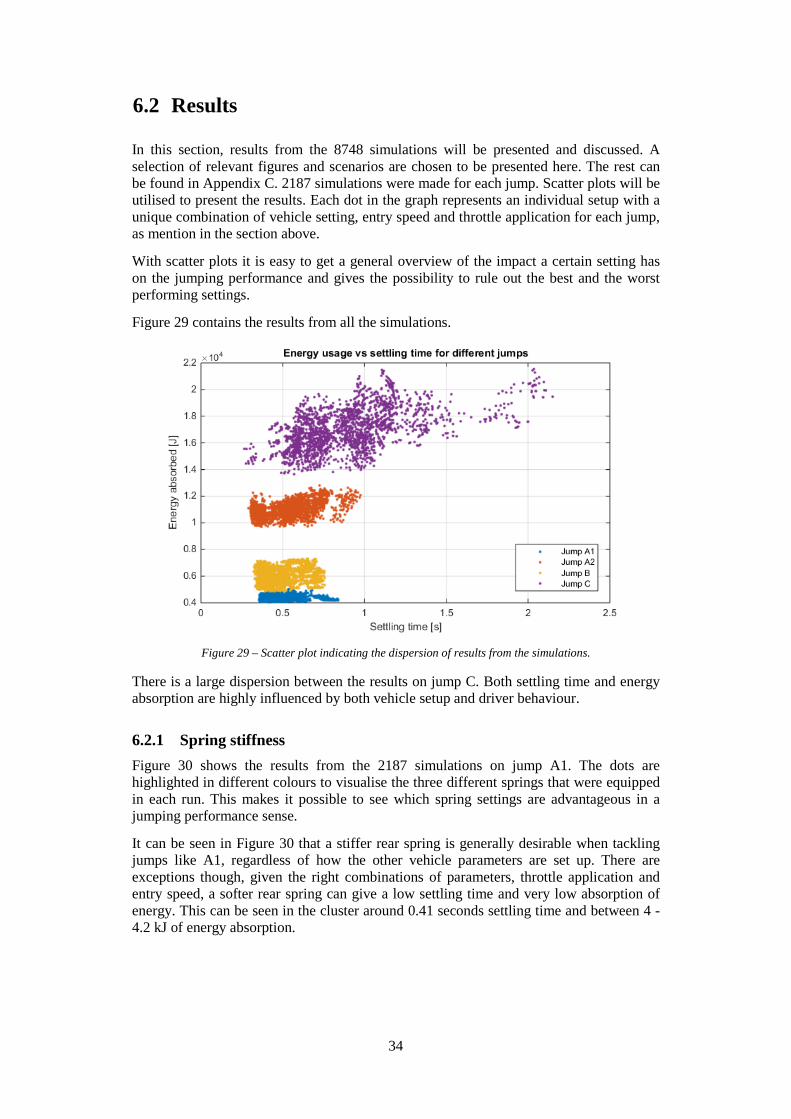
In this section, results from the 8748 simulations will be presented and discussed. A selection of relevant figures and scenarios are chosen to be presented here. The rest can be found in Appendix C. 2187 simulations were made for each jump. Scatter plots will be utilised to present the results. Each dot in the graph represents an individual setup with a unique combination of vehicle setting, entry speed and throttle application for each jump, as mention in the section above. With scatter plots it is easy to get a general overview of the impact a certain setting has on the jumping performance and gives the possibility to rule out the best and the worst performing settings.
Figure 29 contains the results from all the simulations.
Figure 29 – Scatter plot indicating the dispersion of results from the simulations.
There is a large dispersion between the results on jump C. Both settling time and energy absorption are highly influenced by both vehicle setup and driver behaviour.
6.2.1 Spring stiffness Figure 30 shows the results from the 2187 simulations on jump A1. The dots are highlighted in different colours to visualise the three different springs that were equipped in each run. This makes it possible to see which spring settings are advantageous in a jumping performance sense.
It can be seen in Figure 30 that a stiffer rear spring is generally desirable when tackling jumps like A1, regardless of how the other vehicle parameters are set up. There are exceptions though, given the right combinations of parameters, throttle application and entry speed, a softer rear spring can give a low settling time and very low absorption of energy. This can be seen in the cluster around 0.41 seconds settling time and between 4 -4.2 kJ of energy absorption.

35
Figure 30 – Highlighting rear spring stiffness impact on jumping performance on jump A1. Generally a
stiffer rear spring is desirable.
The same phenomenon can be seen on jump C, presented in Figure 31. As in jump A1, a stiffer spring is more desirable overall. Most performance gain can however be made with a softer spring, with the right combinations of settings. Soft rear spring setting appear to work well when combined with stiffer rear dampers and stiffer front springs.
Figure 31 – Highlighting rear spring stiffness impact on jumping performance on jump C. Generally a stiffer rear spring is desirable.
It is more difficult to draw any conclusions about the stiffness on the front springs on all jumps, since the results are evenly distributed in the energy/settling time range. The effect of front spring stiffness is shown for jump B in Figure 32. It is clear that the results are rather dispersed.
36
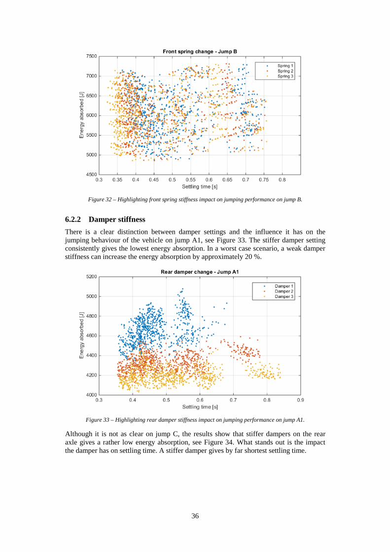
Figure 32 – Highlighting front spring stiffness impact on jumping performance on jump B.
6.2.2 Damper stiffness There is a clear distinction between damper settings and the influence it has on the jumping behaviour of the vehicle on jump A1, see Figure 33. The stiffer damper setting consistently gives the lowest energy absorption. In a worst case scenario, a weak damper stiffness can increase the energy absorption by approximately 20 %.
Figure 33 – Highlighting rear damper stiffness impact on jumping performance on jump A1.
Although it is not as clear on jump C, the results show that stiffer dampers on the rear axle gives a rather low energy absorption, see Figure 34. What stands out is the impact the damper has on settling time. A stiffer damper gives by far shortest settling time.

37
Figure 34 – Highlighting rear damper stiffness impact on jumping performance on jump C.
A stiffer rear damper setting means that the rebound force is larger compared to dampers 1 and 2. Damper 3 is more prone to counteract rear axle “kick-up” on jump C when the vehicle reaches the crest. Lower energy absorption levels are reached due to the decrease in initial pitch rate, made possible by the stiffer damper with a higher rebound force.
As for the front spring stiffness, it is difficult to draw any relevant conclusions regarding front damper stiffness. The influence is rather dispersed which can be seen in Figure 51, Figure 56, Figure 60 and Figure 63 in Appendix C.
6.2.3 Centre of gravity position From the results it can be concluded that a vehicle with the longitudinal position of the centre of gravity in the middle of the car is preferable on the four jumps tested. This is indicated in Figure 35 and Figure 36 and is also backed up by the figures in Appendix C. On jump C it can be seen that a centre of gravity towards the rear of the vehicle is generally not desirable with respect to settling time and energy absorption. There are a few settings and driver behaviour that, combined with a rearward lambda gives poor jumping performance with settling times longer than two seconds.

38
Figure 35 – Highlighting change in centre of gravity position on jump C.
A vehicle with a forward weight distribution performs nearly equally well on jump B as the mid-lambda counterpart, see Figure 36.
Figure 36 – Highlighting change in centre of gravity position on jump B.
The forward centre of gravity position is however sensitive to the type of vehicle setup and driver behaviour as some settings can increase settling time from approximately 0.3 to 0.75 seconds.
6.2.4 Throttle application and entry speed Figure 37 and Figure 38 highlights the influence of driver behaviour on jump B and C. Additional results can be found in Appendix C.

39
Figure 37 – Highlighting the influence of driver behaviour on jump B. LS indicates low speed, MS indicates
medium speed and HS indicates high speed.
Figure 38 – Highlighting the influence of driver behaviour on jump C. LS indicates low speed, MS indicates
medium speed and HS indicates high speed.
What can be concluded from the figures is that the vehicle entry speed has an impact on the energy absorption, which is hardly surprising. However, the settling time for jump A1 (Figure 49), A2 (Figure 53) and B is unaffected by the speed. On jump C it can be seen that a throttle lift off can give a small gain in settling time while 100 % throttle application is mainly preferred on the other jumps to minimise vehicle body movement during landing. When analysing the longest recorded settling times on every jump, it is difficult to point out a single driver behaviour that are responsible for the time increase, the results vary with vehicle setting and the shape of the road profile.
40
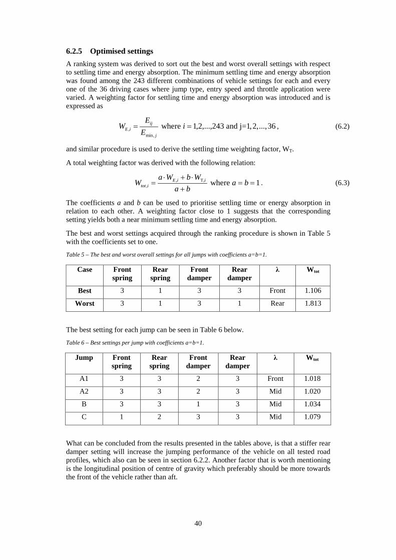
6.2.5 Optimised settings A ranking system was derived to sort out the best and worst overall settings with respect to settling time and energy absorption. The minimum settling time and energy absorption was found among the 243 different combinations of vehicle settings for each and every one of the 36 driving cases where jump type, entry speed and throttle application were varied. A weighting factor for settling time and energy absorption was introduced and is expressed as
,min,
where 1,2,...,243 and j=1,2,...,36ijE i
j
EW i
E= = , (6.2)
and similar procedure is used to derive the settling time weighting factor, WT.
A total weighting factor was derived with the following relation:
, T,, where 1E i i
tot i
a W b WW a b
a b⋅ + ⋅
= = =+
. (6.3)
The coefficients a and b can be used to prioritise settling time or energy absorption in relation to each other. A weighting factor close to 1 suggests that the corresponding setting yields both a near minimum settling time and energy absorption.
The best and worst settings acquired through the ranking procedure is shown in Table 5 with the coefficients set to one.
Table 5 – The best and worst overall settings for all jumps with coefficients a=b=1.
Case Front spring
Rear spring
Front damper
Rear damper
λ Wtot
Best 3 1 3 3 Front 1.106
Worst 3 1 3 1 Rear 1.813
The best setting for each jump can be seen in Table 6 below.
Table 6 – Best settings per jump with coefficients a=b=1.
Jump Front spring
Rear spring
Front damper
Rear damper
λ Wtot
A1 3 3 2 3 Front 1.018
A2 3 3 2 3 Mid 1.020
B 3 3 1 3 Mid 1.034
C 1 2 3 3 Mid 1.079
What can be concluded from the results presented in the tables above, is that a stiffer rear damper setting will increase the jumping performance of the vehicle on all tested road profiles, which also can be seen in section 6.2.2. Another factor that is worth mentioning is the longitudinal position of centre of gravity which preferably should be more towards the front of the vehicle rather than aft.

41
6.3 Additional studies
What could be concluded from the interviews was that the initial speed and throttle and brake application could influence the vehicle behaviour during the jumping phase, see section 2.1. Simulations were made to follow up these conclusions and to further analyse the impact driver behaviour has on the vehicle dynamics.
6.3.1 Throttle application Three identical models were simulated on jump C with different throttle settings; a coasting simulation where the angular velocity of the wheels were constant, a full throttle setting and one throttle lift off setting, see Figure 39. During throttle lift off, a negative torque from the engine decelerates the wheels. The tangential speed of the vehicle was uniform for the three simulation cases. Only inertias which affect the vehicle in the side-vertical plane are considered.
Figure 39 – Pitch angle versus time for different throttle application. The vehicle is airborne between
approximately 0.5 and 1.5 seconds.
It can be seen in Figure 39 that the vehicle pitch angle responds to the velocity and acceleration of the rotating mass. The difference in pitch angle in the landing sequence is approximately 6 degrees between coasting and full throttle application for this particular case. This is significant considering that the vehicle is airborne during approximately one second, which rather short. The difference in pitch angle between full throttle application and throttle lift off when in mid-air is approximately 2 degrees.
This indicates that throttle application is a parameter that highly influences the jumping performance.
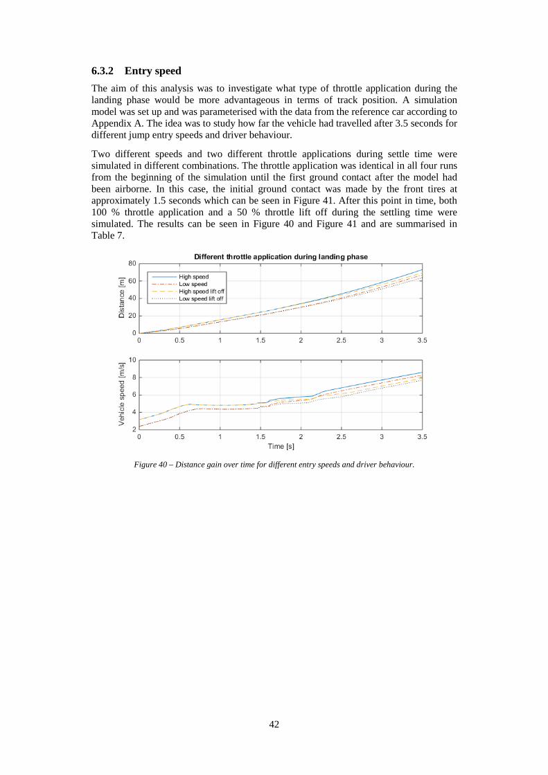
42
6.3.2 Entry speed The aim of this analysis was to investigate what type of throttle application during the landing phase would be more advantageous in terms of track position. A simulation model was set up and was parameterised with the data from the reference car according to Appendix A. The idea was to study how far the vehicle had travelled after 3.5 seconds for different jump entry speeds and driver behaviour.
Two different speeds and two different throttle applications during settle time were simulated in different combinations. The throttle application was identical in all four runs from the beginning of the simulation until the first ground contact after the model had been airborne. In this case, the initial ground contact was made by the front tires at approximately 1.5 seconds which can be seen in Figure 41. After this point in time, both 100 % throttle application and a 50 % throttle lift off during the settling time were simulated. The results can be seen in Figure 40 and Figure 41 and are summarised in Table 7.
Figure 40 – Distance gain over time for different entry speeds and driver behaviour.
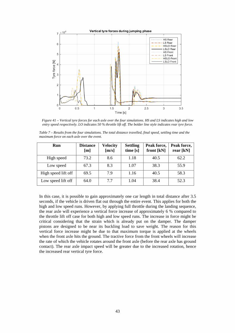
43
Figure 41 – Vertical tyre forces for each axle over the four simulations. HS and LS indicates high and low entry speed respectively. LO indicates 50 % throttle lift off. The bolder line style indicates rear tyre force.
Table 7 – Results from the four simulations. The total distance travelled, final speed, settling time and the maximum force on each axle over the event.
Run Distance [m]
Velocity [m/s]
Settling time [s]
Peak force, front [kN]
Peak force, rear [kN]
High speed 73.2 8.6 1.18 40.5 62.2
Low speed 67.3 8.3 1.07 38.3 55.9
High speed lift off 69.5 7.9 1.16 40.5 58.3
Low speed lift off 64.0 7.7 1.04 38.4 52.3
In this case, it is possible to gain approximately one car length in total distance after 3.5 seconds, if the vehicle is driven flat out through the entire event. This applies for both the high and low speed runs. However, by applying full throttle during the landing sequence, the rear axle will experience a vertical force increase of approximately 6 % compared to the throttle lift off case for both high and low speed runs. The increase in force might be critical considering that the strain which is already put on the damper. The damper pistons are designed to be near its buckling load to save weight. The reason for this vertical force increase might be due to that maximum torque is applied at the wheels when the front axle hits the ground. The tractive force from the front wheels will increase the rate of which the vehicle rotates around the front axle (before the rear axle has ground contact). The rear axle impact speed will be greater due to the increased rotation, hence the increased rear vertical tyre force.

44

45
7 Force build up analysis
How should a spring and damper function to minimise settling time of a vehicle during landing without utilising active control? Position, velocity, acceleration and force are parameters that could perhaps be used to give the spring and/or damper certain characteristics in order to maximise chassis control.
To investigate this, two different types of analyses were made. First, a comparison between how humans and the simulated car absorbs the impact when landing was done. The aim was to study if there are any similarities or non-similarities between car and human jumping and whether it is possible to use any of the human jumping behaviour or force build up strategy when designing dampers. Secondly, a comparison was made between different force build up strategies, where the damper reacts on different inputs to investigate the possibility to improve the jumping performance by adding features to the damper.
7.1 Human comparison
To make an accurate comparison between human force build up and car force build up, measurement data from a human jumping on to a load cell was acquired through Professor Lanie Farewik-Gutierrez at KTH Mechanics. This was measured by having a subject standing on a load cell, jumping up in the air and then again landing on the same load cell. The measurements from the load cell were logged continuously.
The maximum height hmax of the jump is calculated with the known airtime for the subject and the gravitational acceleration, as shown in equation(7.1).
2
max2
2
airtgh
= (7.1)
To compare this to a car, a simulation was set up where the model ran at very high speed on a flat road. After a certain distance, a negative step change was made in the road profile with a height amplitude that corresponded to hmax. The resulting normalised forces, where the forces have been normalised with the objects load at rest, can be seen in Figure 42.

46
Figure 42 – Force build up comparison during landing between a human and a rallycross car.
As shown in Figure 42 the car achieves a higher peak force, probably due to being more limited in the amount of available stroke than the human. The shapes of the curves are very similar, yet scaled differently. The human takes longer to reach steady-state, whilst the car is subjected to higher force levels.
The human subject is also clearly less damped. If the settled state is defined as within 5% of the load at rest, the settling time of the person is almost 1.2 seconds, while the settling time for the car is just above 0.3 seconds. As the human takes almost four times as long to get back to its normal state after impact, trying to take more influence from the human behaviour probably would not increase car jumping performance.
For comparison, data for a human jumping from a stand-still from a higher, determined height was researched. These experiments show a human settling time in the time scale of 0.1-0.3 seconds, indicating that the human setting time is very dependent on individual jumping styles and which type of jump is performed, [14] [15].
In these experiments, it was altogether clear that the shape of the force build-up over time is very similar between the car simulation and the different human measurements.
7.2 Force strategies
To investigate whether there are any other force build-up strategies than the basic force/velocity-based which could be useful for jumping behaviour, a set of other parameters which the damper can react to must be found. These parameters must be indicative to when and only when the car is jumping or landing after a jump. This is due to not wanting to affect damper performance in other areas of operation for the vehicle.
Two ways were thought of for the damper to react to being in a jumping state. The damper can react to being extended fully or at least far enough to be sure that the car is in a jumping state. The damper can also react to the high accelerations which occurs at landing.
Reacting to acceleration has the advantage of being easier to implement as a general idea.
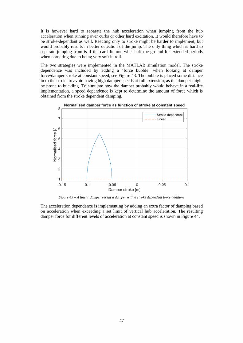
47
It is however hard to separate the hub acceleration when jumping from the hub acceleration when running over curbs or other hard excitation. It would therefore have to be stroke-dependant as well. Reacting only to stroke might be harder to implement, but would probably results in better detection of the jump. The only thing which is hard to separate jumping from is if the car lifts one wheel off the ground for extended periods when cornering due to being very soft in roll.
The two strategies were implemented in the MATLAB simulation model. The stroke dependence was included by adding a ‘force bubble’ when looking at damper force/damper stroke at constant speed, see Figure 43. The bubble is placed some distance in to the stroke to avoid having high damper speeds at full extension, as the damper might be prone to buckling. To simulate how the damper probably would behave in a real-life implementation, a speed dependence is kept to determine the amount of force which is obtained from the stroke dependent damping.
Figure 43 – A linear damper versus a damper with a stroke dependent force addition.
The acceleration dependence is implementing by adding an extra factor of damping based on acceleration when exceeding a set limit of vertical hub acceleration. The resulting damper force for different levels of acceleration at constant speed is shown in Figure 44.

48
Figure 44 – A linear damper versus a damper with an acceleration dependent force addition.
These models were used with the same baseline vehicle parameters as during the parameter study, except with a linear damper as base, not real damper curve. A real damper curve is also used as a benchmark in the comparison. The models are subjected to jump B2, which was chosen as it is a jump where cars typically over-rotate and controlling the vehicle motions when landing is difficult.
Simulations were run at two different speeds, the lower one typical of a real-life jump with a manageable speed and the higher one being so high that damage to the car and/or drivers would be possible. The damper characteristics were tuned in an ad-hoc way, attempting to manually optimise the damper performance by analysing the vehicle behaviour through a series of simulations.
The best results are shown in Table 8 and Table 9 for low and high speeds respectively.
Table 8 - Simulation results for different damper force build-up philosophies at jump B2 and low speed.
Damping type
Settling time [s]
Energy absorbed [J]
Peak front damper force [N]
Peak rear damper force [N]
Linear damper
0.4145 10938 27230 28860
Stroke dependant
0.4355 10954 33510 32190
Acceleration dependant
0.4340 10938 29610 29670
Real damper curves
0.4285 10936 28840 29190
.
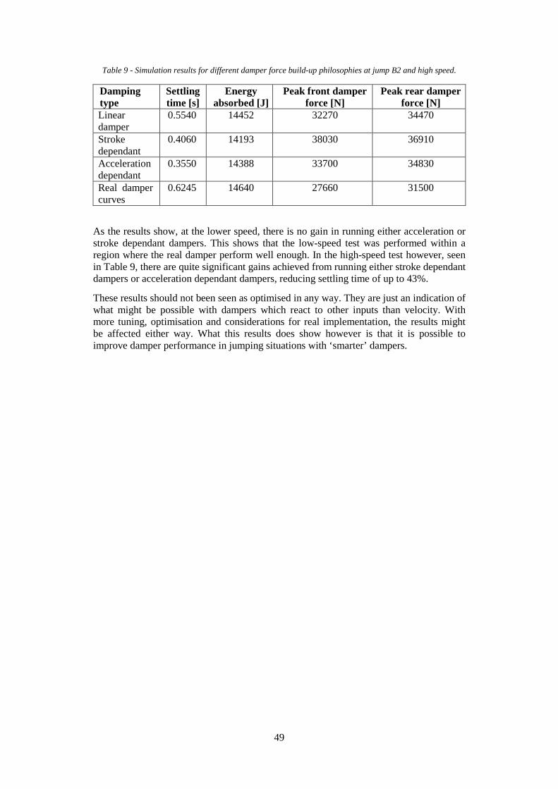
49
Table 9 - Simulation results for different damper force build-up philosophies at jump B2 and high speed.
Damping type
Settling time [s]
Energy absorbed [J]
Peak front damper force [N]
Peak rear damper force [N]
Linear damper
0.5540 14452 32270 34470
Stroke dependant
0.4060 14193 38030 36910
Acceleration dependant
0.3550 14388 33700 34830
Real damper curves
0.6245 14640 27660 31500
As the results show, at the lower speed, there is no gain in running either acceleration or stroke dependant dampers. This shows that the low-speed test was performed within a region where the real damper perform well enough. In the high-speed test however, seen in Table 9, there are quite significant gains achieved from running either stroke dependant dampers or acceleration dependant dampers, reducing settling time of up to 43%.
These results should not been seen as optimised in any way. They are just an indication of what might be possible with dampers which react to other inputs than velocity. With more tuning, optimisation and considerations for real implementation, the results might be affected either way. What this results does show however is that it is possible to improve damper performance in jumping situations with ‘smarter’ dampers.

50
51
8 Discussion
8.1 Evaluation of models
The evaluation of models were performed trying to find aspects where the four different simulation models differed. In general, the trends were quite similar between all of the simulations when it comes to the simulated utilised stroke and stroke velocities. Both MATLAB and CarSim generally overestimated the wheel displacements and displacement rates. Amesim consistently underestimated these quantities but together with MATLAB it managed to predict the correct pitch motion on all jumps. Many of the reasons as to why the simulations differed in the simulations will remain unclear as the models used in the two commercial alternatives are unknown. For the MATLAB model it could be considered that all of the losses in the suspension movement is in the dampers or the bump stop, whereas the real vehicle has friction in every joint which is hard to measure or estimate as well as implement in the model, as the friction will vary depending on the load on each joint.
It is arguably preferable to have a model which slightly overestimates rather than underestimates the stroke and displacement speed when designing, as a two-dimensional model never can take roll angles when landing in to account. The springs and dampers needs to be able to handle a worst-case scenario where the car lands with a large roll angle, which in turn will require stiffer dampers and springs than a symmetrical landing in the y-plane.
When investigating the usability of the models it was quickly found that ADAMS/Car was not easy enough to parameterise vehicle models in for our need and was therefore excluded from the rest of the study as it simply takes too much time to use.
The CarSim model is easy enough to parameterise to be quick and useful and the GUI is clear and concise. The post processing is made easy and the animation tool is intuitive. The largest drawback in terms of usability is that it lacks customisability for non-velocity based damper and non-linear tires. The solution to this issue is to involve other software to couple to CarSim to fully simulate the dynamics of the system. This will most likely increase the expenditure of time to set up and simulate a model which departs from the discussed software criteria.
Amesim provided ample usability and the basic iCar interface was simple enough for a simulation to be run fairly quickly. The kinematics and compliance application can help the user to create look-up tables for suspension properties if certain static values e.g. roll centre height at design load, initial camber and camber gain. However, as soon the model needs to be modified for implementation of non-velocity based damper for instance, the model has to be modified by using other Amesim components than those already implemented, which is not a trivial process.
The MATLAB based model has, with the developed GUI, been customised to take most, if not all, of the situations which will be required to analyse jumping behaviour quickly. Most of the parameter sets are already configured for different types of cars and the important parameters are easy to change. Non-linear bump stops and springs as well as the possibility of non-velocity based dampers are implemented. Road profiles are easy to create, alter, save and reuse. The results are easy to visualise and analyse.
Without the GUI, the MATLAB model would have been more difficult to use, as it would

52
have been script based. This would require very good documentation and a fair bit of time to learn to use the scripts. This is the main reason for developing and implementing the GUI for usability, while keeping the script based version for fully customisability for future eventualities.
Combining all of these features, drawbacks and results, the MATLAB model was chosen for the continuation of this study as it provides the best solution for the current needs, from precision and usability to features and software licensing.
8.2 Parameter study
The parameter study was performed using only the MATLAB model. The parameters were varied in steps which were based on the real setup of the vehicle analysed. This produced a test matrix which was run through.
It would have been possible to extend this test setup to include further parameters to test. Other properties which are known by experience to affect jumping behaviour is spring preload, available damper stroke and tyre stiffness. It would also have been interesting to alter the damper characteristics in only one speed range, instead of altering all speed ranges at the same time. This was not done fully due to the time and effort required to perform all those simulations and perform the analysis of the simulation data.
One consideration which was not made, was to tune the spring stiffness to match axle frequencies when changing the centre of gravity position. However, the spring settings tested made sure that a reasonable stiffness for each centre of gravity configuration was still tested.
Based on the results it is clear that for these cars, the rear suspension setup seem to be more important to jumping performance than front setup. For better jumping performance, the rear suspension should be stiffened, which appears to be consistent for all of the different jump and velocity cases.
None of the setup suggestions have been tested on a real car and it might be the case that the suggested changes hurts performance in other areas on track. Therefore, the ideas mentioned in the force build-up chapter about stroke or acceleration dependant damping will be very helpful when implementing these damper changes in reality, as they are only active when a jump is detected while being unchanged in other areas on track.
8.3 Force build up
During the first part of the force build up analysis inspiration is taken from nature, trying to replicate the behaviour of a human landing. It is possible that this section would have been more useful had it been for two reasons.
Firstly, a human is arguably not the perfect creature to compare with and take inspiration from, as the jumping capacity of a human is hardly ideal compared with many animals if comparing body length to maximum fall height. It would perhaps have been more fruitful to analyse the jumping behaviour of a cat or a cheetah. During the course of the creation of this thesis, discussions were held about doing this type of analysis on a cat’s jumping behaviour. However, it fell through due to the required measuring equipment which was

53
available was located at a children’s hospital. This meant that it was not possible to bring a cat there due to the allergy risks.
Secondly, it would also have been preferable to have a wider set of data to analyse, with a larger set of different jumps from different heights as well as a few forward leaps to investigate if there are different types of force build-ups in different movements and to study what happens when the jump height increases.
The second part of the force build up analysis deals with utilising dampers which react to other inputs than displacement speed. Although it is clear that reacting to acceleration or stroke position might increase jumping performance in this particular case, it might not be the case for all of the different jumps. Before implementing such a function in a real damper, it would have to be further investigated which downsides there are. As shown in the results, it does hurt settling time a small amount compared to linear or normal dampers when it comes to non-extreme jumps which might indicate loss of performance in other regions.
It would also have to be investigated whether or not the mentioned ways of implementing stroke or acceleration based dampers is the best way of doing so. There is a lot of tuning, testing and optimisation which can be made to the force build up strategy which has not been done here.

54

55
9 Conclusion
The jumping performance of rallycross cars were to be investigated, due to problems with landing with unfavourable pitch angles, hampering car performance or cause damage on the cars themselves. Drivers and race engineers were interviewed to investigate what they thought was the problem with the jumping performance and what they did to deal with it. Rallycross tracks were measured using RTK GPS equipment to give the road profiles of jumps and data from real cars were collected. The vertical stiffness of rallycross tyres were measured.
Vehicle models in LMS Amesim, CarSim, ADAMS/Car and a MATLAB model were evaluated for jumping performance against a decided set of criteria, covering precision, usability, time consumption and expandability. ADAMS/Car was excluded early due to high time consumption. CarSim and Amesim was found adequate for performance and time consumption but lacking in usability and expandability. The MATLAB model was used to perform the following analysis and a graphical user interface was developed for it.
Five different vehicle parameters, front/rear spring stiffness, front/rear damper stiffness and centre of gravity position were evaluated in a parameter study where the simulated vehicle was run over four different jumps at three different speeds. Not all results were consistent over all jumps, but some general trends were clear. Rear damper stiffness and rear spring stiffness were found to be two very important tools for tuning a vehicle’s jumping performance, as well as driver throttle behaviour. The difference in vehicle settling time can vary between below 0.4 to above 2 seconds on the same jump, depending on the tuning of these parameters.
A force build-up analysis was made, where a comparison between a human’s force build-up and the simulated vehicles. It was concluded that the force build-up was similar, yet the human appears less damped with longer settling time.
Different damper force build-up strategies were also tested with dampers reacting to acceleration and stroke position. It was found that damper which reacts to either stroke or acceleration and increases damper force when highly extended or under high acceleration has the possibility to reduce vehicle settling time with up to 45%.

56
57
10 Future work
To improve on this work, further parameter studies could be performed, where additional parameters are tested, such as spring preload, damper stroke and tyre characteristics. Already tested parameters should be fine-tuned, with tighter windows for spring and damper stiffness, trying to find more optimal configuration.
Further damper analysis should be performed, evaluating in which direction and at what speed added damping could help jumping performance.
The force build-up strategies should be developed further, trying to determine a ‘sweet spot’ for the stroke or acceleration reaction. This should be done with a real-world connection to implementation in dampers and how the force build-up in real dampers would work.
Additional tests should be performed with a real car on track, verifying the behaviour and response found in the simulations as well as testing the optimised setups found.

58
59
11 References
[1] Rallycross Driver 1, Interviewee, Vehicle Jumping Behaviour and How to Manage It. [Interview]. 18 June 2014.
[2] Rallycross Engineer 1, Interviewee, Vehicle Jumping Behaviour and How to Manage It. [Interview]. 1 July 2014.
[3] “SWEPOS,” [Online]. Available: https://swepos.lantmateriet.se/tjanster/realtid/natverksrtk/matosakerhet.aspx. [Accessed 7 August 2014].
[4] “Lantmäteriet,” [Online]. Available: http://www.lantmateriet.se/sv/Kartor-och-geografisk-information/GPS-och-geodetisk-matning/GPS-och-satellitpositionering. [Accessed 7 Augusti 2014].
[5] R. K. Taylor, L. L. Bashford and M. D. Schrock, “Methods for Measuring Vertical Tyre Stiffness,” American Society of Agricultural Engineers, Kansas, 2000.
[6] J. A. Lines and K. Murphy, “The Stiffness of Agricultural Tractor Tyres,” Journal of Terramechanics, vol. 28, pp. 49-64, 1991.
[7] Yokohama Rubber Company, Tyre data sheet, Yokohama Rubber Company, 2012. [8] “CarSim,” [Online]. Available: http://www.carsim.com/products/carsim/index.php. [Accessed 5
August 2014]. [9] “MSC Software,” [Online]. Available: http://www.mscsoftware.com/application/multibody-
dynamics. [Accessed 4 August 2014]. [10] MSC.ADAMS, “Getting Started Using ADAMS/Car,” 7 November 2014. [Online]. Available:
https://simcompanion.mscsoftware.com/infocenter/index?page=content&id=DOC9781&actp=LIST. [Accessed 23 February 2015].
[11] KTH, Division of Aeronautical & Vehicle Engineering, Vehicle Dynamics, Stockholm, 2011. [12] MathWorks, “Tire-Road Interaction (Magic Formula),” [Online]. Available:
http://se.mathworks.com/help/physmod/sdl/ref/tireroadinteractionmagicformula.html. [Accessed 03 03 2015].
[13] Öhlins Racing AB, “ORQ 18/50,” 2015. [Online]. Available: http://www.ohlins.com/product/orq-1850/. [Accessed 03 March 2015].
[14] P. Devita and S. A. William, “Effect of landing stiffness on joint kinetics and energetics in the lower extremity,” Medicine and Science in Sports and Exercise, vol. 224, no. 1, pp. 118-115, 1992.
[15] J. T. Weinhandl, J. D. Smith and E. L. Lugan, “The Effects of Repetitive Drop Jumps on Impact Phase Joint Kinematics and Kinetics,” Journal of Applied Biomechanics, no. 27, pp. 108-115, 2011.

60

61
Appendix A – Vehicle data
The vehicle properties that were used to parameterise the simulation models can be seen in Table 10 and Table 11.
Table 10 – Table of data for the reference car
Mass [kg] 1200
Unsprung mass [kg] 50
Wheel base [mm] 2500
CoG x-position, distance to rear axle [mm] 1100
Pitch inertia [kgm2] (estimated) 1300
Interia, tyre [kgm2] (estimated) 2.5
Table 11 – Specified setup of the reference car during tests on track A and B
Tyre vertical stiffness [N/mm] 320
Spring stiffness, front [N/mm] 65
Spring stiffness, rear [N/mm] 70
Assist spring stiffness [N/mm] 15
Equivalent stiffness bump stop, front [N/mm] 250
Equivalent stiffness bump stop, rear [N/mm] 250
Wheel travel [mm] 240
Motion ratio front, full compression 0.83
Motion ratio front, full rebound 0.52
Motion ratio rear, full compression 0.77
Motion ratio rear, full rebound 0.50

62

63
Appendix B – Model validation
Results from the validation on jump A2 are presented in the figures below.
Figure 45 – Front wheel displacement on jump A2.
Figure 46 – Front wheel displacement rate on jump A2.

64
Figure 47 – Rear wheel displacement on jump A2.
Figure 48 – Rear wheel displacement rate on jump A2. The rear right wheel displacement rate is not shown
due to faulty sensor.

65
Appendix C – Parameter study
The result from the parameter study will be presented in the figures below.
Figure 49 – Highlighting influence of driver behaviour on jump A1.
Figure 50 – Highlighting front spring change on jump A1

66
Figure 51 – Highlighting front damper change on jump A1.
Figure 52 – Highlighting change in longitudinal position of centre of gravity on jump A1.
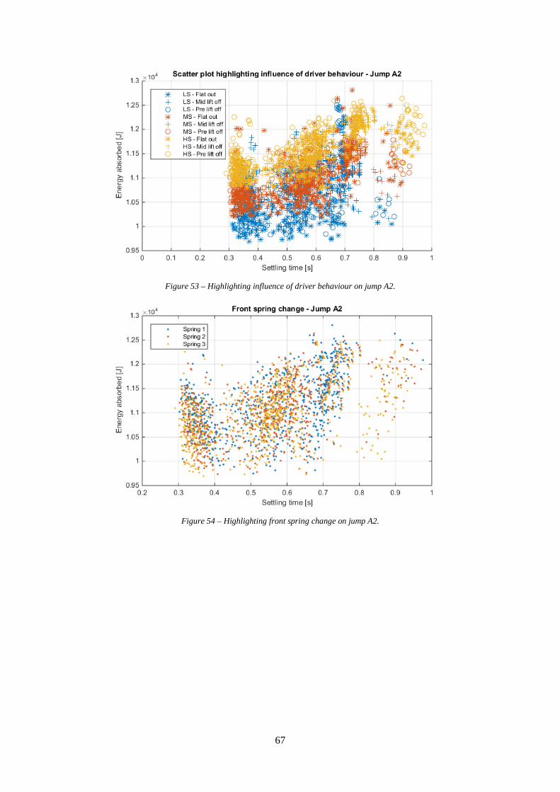
67
Figure 53 – Highlighting influence of driver behaviour on jump A2.
Figure 54 – Highlighting front spring change on jump A2.
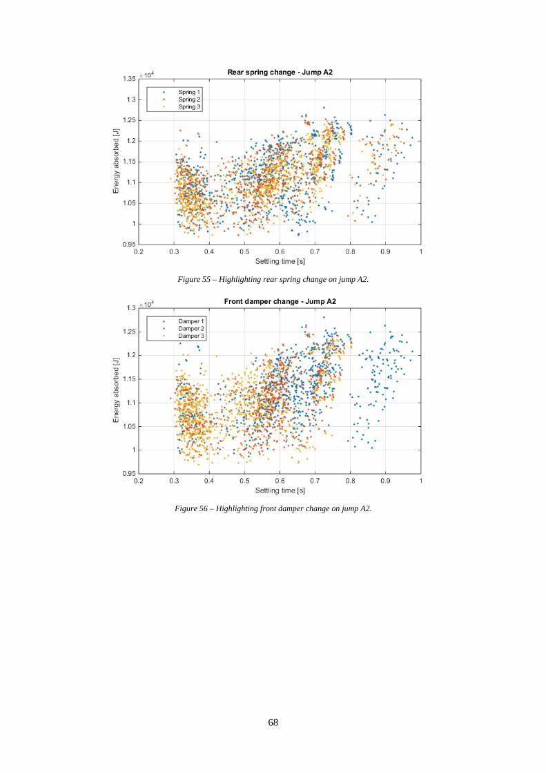
68
Figure 55 – Highlighting rear spring change on jump A2.
Figure 56 – Highlighting front damper change on jump A2.

69
Figure 57 – Highlighting rear damper change on jump A2.
Figure 58 – Highlighting change in longitudinal position of the centre of gravity on jump A2.
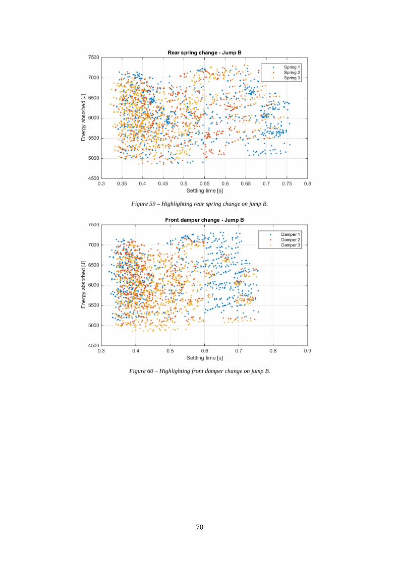
70
Figure 59 – Highlighting rear spring change on jump B.
Figure 60 – Highlighting front damper change on jump B.
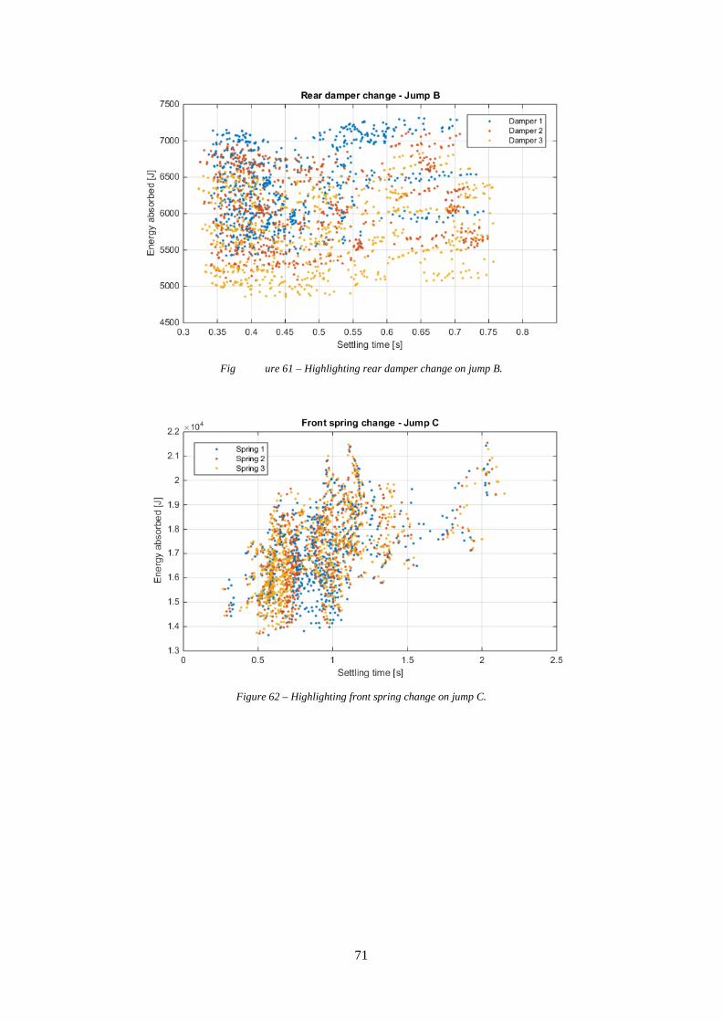
71
Fig ure 61 – Highlighting rear damper change on jump B.
Figure 62 – Highlighting front spring change on jump C.

72
Figure 63 – Highlighting front damper change on jump C.