vehicle dynamic modelling and parameter identification for
TRANSCRIPT

Vehicle Dynamic Modelling and Parameter Identification for an
Autonomous Vehicle
by
Matthew Van Gennip
A thesis
presented to the University of Waterloo
in fulfillment of the
thesis requirement for the degree of
Master of Applied Science
In
Systems Design Engineering
Waterloo, ON, Canada, 2018
© Matthew Van Gennip 2018

ii
Author’s Declaration
I hereby declare that I am the sole author of this thesis. This is a true copy of the thesis, including
any required final revisions, as accepted by my examiners.
I understand that my thesis may be made electronically available to the public.

iii
Abstract
For autonomous vehicles to be feasible, a fast and accurate model of the vehicle dynamics is
required due to the complexity of the task. There are many different aspects to a driverless vehicle,
including path planning, image processing, data analysis, and the low level control of the vehicle. All these
processes are important; they need to work in tandem for the vehicle to be able to drive itself. Regardless
of how good all the components are, the vehicle itself must be able to follow the desired trajectory. This
is accomplished through the low level control of the vehicle, by using an accurate vehicle dynamic model
to assess the safety and feasibility of a given trajectory. This thesis develops a 14 degree of freedom full
car model of a 2015 Lincoln MKZ hybrid vehicle. A vehicle measurement system is attached to the vehicle
in order to measure the suspension displacement along with the tire orientation, velocities, forces, and
moments. In addition, a GPS and an inertial measurement unit is used to measure the position,
acceleration, and angular velocities of the chassis. The vehicle is then tested on a dedicated test track in
order to identify the vehicle parameters. The center of mass, wheel and vehicle inertias, coefficient of
drag, and suspension parameters are identified. In addition, combined slip Pacejka tire models are
developed. These parameters are identified using a two-step process. Parameters are first identified using
simple physics based models. The second step uses the full vehicle dynamic model to further optimize the
parameters, accounting for the numerous simplifications assumed in the simple physics based models.
The vehicle dynamic model is implemented and validated in MapleSim 2017.3. The model is intended to
be used for controller development and autonomous vehicle testing in a simulation environment.

iv
Acknowledgements
The author would like to thank Maplesoft, the Natural Sciences and Engineering Research Council
of Canada, the Canada Research Chairs Program, and the Ontario Centres of Excellence for funding this
research.

v
Table of Contents
Author’s Declaration ...................................................................................................................... ii
Abstract ........................................................................................................................................ iii
Acknowledgements ...................................................................................................................... iv
Table of Contents .......................................................................................................................... v
List of Figures .............................................................................................................................. vii
List of Tables ................................................................................................................................. ix
List of Abbreviations ...................................................................................................................... x
List of Symbols .............................................................................................................................. xi
1. Introduction and Literature Review ...................................................................................... 1
1.1. Introduction ................................................................................................................. 1
1.2. Thesis Organization ...................................................................................................... 2
1.3. Literature Review ......................................................................................................... 3
1.3.1. Parameter Identification ........................................................................................... 3
1.3.2. Tire Modelling........................................................................................................... 6
2. Data Collection and Experimental Testing........................................................................... 12
2.1. Data Acquisition System ............................................................................................. 12
2.1.1. Vehicle Measurement System ................................................................................. 12
2.1.2. VBOX 3i ................................................................................................................... 16
2.1.3. Vehicle CAN and Vehicle Control Module ................................................................ 17
2.2. Experimental Testing .................................................................................................. 18
2.2.1. Center of Mass Tests ............................................................................................... 18
2.2.2. Inertia Tests ............................................................................................................ 20
vi
2.2.3. Coefficient of Drag and Rolling Resistance Tests ...................................................... 22
2.2.4. Suspension Tests..................................................................................................... 23
2.2.5. Tire Tests ................................................................................................................ 25
3. Vehicle Dynamic Modeling and Parameter Identification .................................................... 28
3.1. Modelling ................................................................................................................... 28
3.2. Parameter Identification Using Simple Models ............................................................ 30
3.2.1. Center of Mass........................................................................................................ 30
3.2.2. Inertias ................................................................................................................... 36
3.2.3. Coefficient of Drag and Equivalent Rolling Resistance ............................................. 40
3.2.4. Suspension ............................................................................................................. 47
3.2.5. Tire Modelling......................................................................................................... 55
3.3. Parameter Identification Using High Fidelity Vehicle Dynamic Model .......................... 67
4. Full Model Validation ......................................................................................................... 68
4.1. Longitudinal Validation ............................................................................................... 68
4.2. Lateral Validation ....................................................................................................... 74
4.3. Combined Validation .................................................................................................. 79
5. Conclusions ........................................................................................................................ 84
5.1. Summary .................................................................................................................... 84
5.2. Future Work ............................................................................................................... 84
References .................................................................................................................................. 86
Appendix A – MapleSim Model Picture ........................................................................................ 91
Appendix B – Final Parameter Values ........................................................................................... 93
vii
List of Figures
Figure 1.1: Sideslip angle definition ................................................................................................ 7
Figure 1.2: Society of Automotive Engineers (SAE) tire axis definition [33] ................................... 10
Figure 2.1: The Moose at the Waterloo Test Track with the VMS ................................................. 12
Figure 2.2: Wheel Force Sensor (WFS) attached to custom wheel rim .......................................... 13
Figure 2.3: Wheel Position Sensor (WPS) ..................................................................................... 14
Figure 2.4: Laser Ground Sensor (LGS) ......................................................................................... 15
Figure 2.5: Experimental setup for static test to determine the height of the center of mass ....... 18
Figure 2.6: Velocity versus time for the center of mass dynamic maneuver .................................. 19
Figure 2.7: Wheel speed/torque versus time ............................................................................... 20
Figure 2.8: Lincoln MKZ at Waterloo International Airport for drag testing .................................. 22
Figure 2.9: Lincoln MKZ on 4-post test rig .................................................................................... 23
Figure 2.10: Sample vehicle trajectory of the grand sweep maneuver .......................................... 27
Figure 3.1: Defined location of the vehicle center of mass ........................................................... 30
Figure 3.2: Experimental setup for static test to determine the height of the center of mass ....... 32
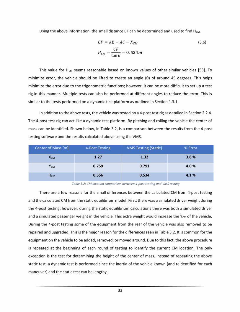
Figure 3.3: HCM versus time for dynamic maneuver ...................................................................... 34
Figure 3.4: Wheel moment of inertia versus time ........................................................................ 36
Figure 3.5: Free body diagram of the vehicle during a longitudinal maneuver .............................. 37
Figure 3.6: Front Profile of the Lincoln MKZ ................................................................................. 41
Figure 3.7: Frontal area of the Lincoln MKZ .................................................................................. 41
Figure 3.8: Resistive forces for uphill maneuver ........................................................................... 44
Figure 3.9: Resistive forces for downhill maneuver ...................................................................... 45
Figure 3.10: Dimensionless velocity versus time comparison between experimental results and
simulated model ................................................................................................................................... 46
Figure 3.11: Suspension model for 4-post testing ......................................................................... 47
Figure 3.12: Free body diagram of one tire .................................................................................. 48
Figure 3.13: Damping force versus rate of change of suspension compression ............................. 49
viii
Figure 3.14: Non-linear behaviour of suspension spring ............................................................... 50
Figure 3.15: Damping force versus rate of change of suspension compression (non-linear spring) 51
Figure 3.16: Change in wheel height over time ............................................................................ 52
Figure 3.17: Lateral position of the wheel with respect to the vertical position of the wheel ........ 53
Figure 3.18: Camber angle of the wheel with respect to the vertical position of the wheel .......... 54
Figure 3.19: Toe angle of the wheel with respect to the vertical position of the wheel ................. 54
Figure 3.20: Measured longitudinal force for rear wheel .............................................................. 56
Figure 3.21: Measured data from pure longitudinal slip test ........................................................ 57
Figure 3.22: Normalized longitudinal force versus pure longitudinal slip ...................................... 58
Figure 3.23: Normalized lateral force versus pure sideslip ............................................................ 59
Figure 3.24: Visualization of the friction ellipse ............................................................................ 61
Figure 3.25: Normalized longitudinal force versus normalized lateral force .................................. 62
Figure 3.26: Longitudinal slip versus normalized longitudinal force with varying sideslip .............. 63
Figure 3.27: Combined slip Pacejka models for sideslip values of 0, 10, and 20 degrees ............... 65
Figure 3.28: Longitudinal Pacejka tire models for sideslip values between 0 and 25 degrees ........ 66
Figure 4.1: Trajectory for longitudinal validation .......................................................................... 68
Figure 4.2: Longitudinal velocity versus time for longitudinal validation ....................................... 69
Figure 4.3: Accelerations versus time for longitudinal validation .................................................. 71
Figure 4.4: Angular velocities versus time for longitudinal validation ........................................... 72
Figure 4.5: Trajectory for lateral validation .................................................................................. 74
Figure 4.6: Longitudinal velocity versus time for lateral validation ............................................... 75
Figure 4.7: Accelerations versus time for lateral validation .......................................................... 76
Figure 4.8: Angular velocities versus time for lateral validation .................................................... 77
Figure 4.9: Trajectory for combined validation ............................................................................. 79
Figure 4.10: Longitudinal velocity versus time for combined validation ........................................ 80
Figure 4.11: Accelerations versus time for combined validation ................................................... 81
Figure 4.12: Angular velocities versus time for combined validation ............................................ 82
Figure A.1: Visual Representation of Full Vehicle Dynamic Model ................................................ 91
Figure A.2: Schematic of the Full Vehicle Dynamic Model ............................................................ 92

ix
List of Tables
Table 3.1: Summary of the model inputs and outputs .................................................................. 29
Table 3.2: CM location comparison between 4-post testing and VMS testing ............................... 33
Table 3.3: Comparison of CM locations over time ........................................................................ 35
Table 3.4: Suspension parameter identification using data from 4-post testing ............................ 48
Table B.1: Final parameter values for the Moose ......................................................................... 93
Table B.2: Combined slip longitudinal Pacejka model parameters ................................................ 94
Table B.3: Combined slip lateral Pacejka model parameters ......................................................... 94
x
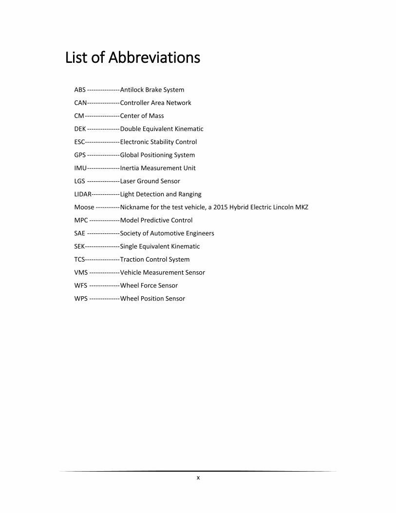
List of Abbreviations
ABS --------------- Antilock Brake System
CAN --------------- Controller Area Network
CM ---------------- Center of Mass
DEK --------------- Double Equivalent Kinematic
ESC ---------------- Electronic Stability Control
GPS --------------- Global Positioning System
IMU --------------- Inertia Measurement Unit
LGS --------------- Laser Ground Sensor
LIDAR------------- Light Detection and Ranging
Moose ----------- Nickname for the test vehicle, a 2015 Hybrid Electric Lincoln MKZ
MPC -------------- Model Predictive Control
SAE --------------- Society of Automotive Engineers
SEK ---------------- Single Equivalent Kinematic
TCS ---------------- Traction Control System
VMS -------------- Vehicle Measurement Sensor
WFS -------------- Wheel Force Sensor
WPS -------------- Wheel Position Sensor

xi
List of Symbols
g ------------------- Gravity
m ------------------ Mass
�⃑�------------------- Velocity
�⃑�------------------- Acceleration
I -------------------- Inertia
M ------------------ Moment
�⃑� ------------------ Force
𝜏 ------------------- Torque
�⃑⃑⃑� ------------------ Angular speed
�̇⃑⃑⃑� ------------------ Angular acceleration
μR ----------------- Coefficient of rolling resistance
Ρ ------------------- Density of air
Cd ------------------ Coefficient of drag
Af ------------------ Frontal area
l0 ------------------ Un-sprung length of suspension
k ------------------- Spring constant
c ------------------- Damping coefficient
RTire --------------- Tire radius
s ------------------- Longitudinal slip
α ------------------- Wheel sideslip
Cx ------------------ Longitudinal stiffness of the wheel
CY ------------------ Cornering stiffness of the wheel
B, C, D, E --------- Pacejka tire model parameters
μx ------------------ Coefficient of friction in the longitudinal direction
μy ------------------ Coefficient of friction in the lateral direction
Q1, Q2, Q3-------- Overturning moment parameters
γ ------------------- Camber angle

xii
XWheelBase --------- Distance from the front axle to the rear axle
XWheelTrack --------- Distance from the center of the left wheel to the center of the right wheel
XCM ---------------- Distance from the front axle to the center of mass
YCM ---------------- Distance from the centerline of the left wheel to the center of mass
HCM --------------- Distance from the ground to the center of mass
WRear -------------- Weight measured by the WFS on the two rear wheels
WFront ------------- Weight measured by the WFS on the two front wheels
WRight ------------- Weight measured by the WFS on the two right wheels
WLeft -------------- Weight measured by the WFS on the two left wheels
WCM --------------- Weight measured by the WFS on all four wheels

_______________________________________________________________________________________
1 Metro Magazine, ”NAVYA, Keolis to operate autonomous shuttle on public roads”. August 13, 2018. http://www.metro-magazine.com/technology/news/730846/navya-keolis-to-operate-autonomous-shuttle-on-public-roads 2 Hetzner, Christiaan, “Germany seeks to create self-driving infrastructure”. August 10, 2018. http://www.autonews.com/article/20180810/COPY01/308109968/germany-seeks-to-create-self-driving-infrastructure 3 Banerjee, A., Lienert, P., Shepardson, D., “Ford follows GM’s Cruise move with self-driving spinoff”. July 24, 2018. https://www.reuters.com/article/us-ford-motor-autonomous/ford-follows-gms-cruise-move-with-self-driving-spinoff-idUSKBN1KE24P 4 Aptiv PLC, “Aptiv Launches Fleet of Autonomous Vehicles on the Lyft Network”. May 02, 2018. https://www.prnewswire.com/news-releases/aptiv-launches-fleet-of-autonomous-vehicles-on-the-lyft-network-
300640756.html
1
1. Introduction and Literature Review
1.1. Introduction
Autonomous vehicles are getting much attention these days.1, 2, 3, 4 There are many different parts
of a driverless vehicle, including path planning [1], image processing [2-4], data analysis, and the low level
control of the vehicle [5]. All these processes are important; they need to work in tandem for the vehicle
to be able to drive itself. Regardless of how good all the components are, the vehicle itself must be able
to follow the desired trajectory. This can be accomplished by using an accurate vehicle dynamic model to
assess the safety and feasibility of a given trajectory [6].
An accurate vehicle dynamic model has many different benefits when developing an autonomous
vehicle [7-8]. One benefit, as stated above, is that it could be used to determine whether a trajectory is
feasible or not. Another benefit is that it can be reduced and used as a control oriented model. Yet another
benefit is the ability to incorporate the full model into a simulation environment in order to accurately
test how the vehicle will react under many different circumstances. This is easier and much safer than
having to test the vehicle on real roads.
There is an ongoing project at the University of Waterloo that is working to convert a 2015 Hybrid
Electric Lincoln MKZ (nicknamed the Autonomoose, or Moose for short) into a fully autonomous vehicle.
One subsection of this project is dedicated to creating a high-fidelity model of the Moose that can be used
for testing in a simulation environment. This thesis covers the vehicle dynamic modeling and parameter
identification necessary for this project.
2
1.2. Thesis Organization
This thesis details the testing, modelling, and parameter identification of a full 14 degree of freedom
vehicle dynamic model for use in simulation, testing, and controller development. The first chapter
consists of an overview and literature review of the parameter identification methods and current state
of the art. The second chapter details the measurement devices used for data collection along with a
detailed description of the different tests that were performed. The third chapter describes the structure
of the model and the parameter identification performed. The fourth chapter presents the validation
results for the full model under longitudinal, lateral, and combined scenarios. Lastly, the thesis concludes
with several observations and suggestions for future work.

3
1.3. Literature Review
1.3.1. Parameter Identification
To create a realistic vehicle dynamic model, many important vehicle parameters must be identified.
The accuracy of these parameters affects the accuracy of the model. Based on the intended fidelity of the
model, many parameters can be ignored. For instance, a single-track model ignores all pitching and rolling
effects, including all suspension parameters, corresponding inertia parameters, and the center of gravity
locations associated with these effects. This simplifies the complexity of the model greatly; however it
also limits the uses of the model due to the simplicity.
For the 14 degree of freedom model developed in this thesis, there are many parameters to
identify. There is the center of mass location, the inertia of the vehicle and the tires, the coefficient of
drag, all the suspension parameters, and all necessary tire parameters. Due to the complexity of the tire
model parameters, these will be discussed in Section 1.3.2.
To estimate parameters for a high fidelity model, it is often easier to investigate how the
parameters would be identified for lower fidelity models. For instance, when looking at the inertial
parameters of the vehicle, if a high fidelity model is used then any error in other identified parameters
can lead to errors in the inertial parameters. Consequentially, many parameters are derived from first
principles or simplified models that isolate the desired parameters. By using this method, many
simplifications can be assumed. This leads to parameters that are slightly erroneous due to the
simplifications. To account for this inaccuracy, after all parameters are identified they are implemented
in the full vehicle dynamic model where further optimization can occur. This optimization will tweak the
parameters, correcting the earlier simplifications.
The center of mass (CM) is a point representing the mean position of matter in the vehicle. The CM
of a vehicle can be found in many ways [9-11]. Generally the CM is found statically on a fixed test platform.
This method is simple and reliable, using first principles, namely moment balance equations, to determine
the horizontal CM location by recording the weight on each wheel. The height of the CM can be found
using the same principles; however in order to do this the vehicle must be tilted or rolled so that the
vehicle is no longer horizontal. Generally this value is found by using a dynamic test platform which can
rotate the vehicle slowly. It can also be found during a dynamic maneuver involving vehicle pitching

4
maneuvers. Lacking the equipment to perform this test, the vehicle can be statically placed in a non-
horizontal orientation in order to determine the CM, although this method is less accurate due to limited
experimental data – only having one data point as opposed to an array of data points that would be
obtained using a dynamic test platform.
The inertia parameters represent the resistance of the vehicle to any change in velocity. These
parameters can be found in many different ways [12]. One of the more accurate methods to determining
the inertia of a vehicle is by using a dynamic test platform to perform a series of maneuvers that excite
isolated rolling, pitching, and yawing motions of the vehicle [13-14]. By isolating the desired motion, a
simple moment balance equation can be used. This sort of testing can accurately determine the principal
moments of inertia. Additional testing can be completed in a similar manner to determine the products
of inertia; however, due to the near symmetry of the vehicle these values are usually small and generally
ignored [15].
Another method to determine the inertia of a vehicle is by performing dynamic maneuvers and
measuring the angular velocities and accelerations along with the forces on the vehicle. This method is
not as accurate due to the difficulty in isolating pitching, rolling, and yawing motions. In addition, the
forces experienced by the vehicle are generally difficult to measure accurately. If the forces are measured
accurately then a full set of moment balance equations can be used to identify the inertial parameters.
Even though the measurement accuracy is reduced, by optimizing all parameters simultaneously a more
accurate result may be achieved.
The drag force on a vehicle is a force that acts opposite to the relative motion between the air and
the vehicle. It is common for automotive manufactures to design a streamlined vehicle that minimizes the
drag force by minimizing the coefficient of drag for the vehicle. The coefficient of drag is easiest to identify
in a wind tunnel due to the level of control available [16]. In a wind tunnel, the wind speed and direction
is defined and controlled as an input. On a test track, the wind speed and direction are difficult to
determine accurately. By measuring the forces experienced on the vehicle while measuring the speed of
the wind relative to the chassis, the drag coefficient can be identified. This can also be done through on-
road testing [18]; however as mentioned before, the relative speed between the wind and the chassis can
be difficult to measure experimentally. Measuring the relative speed is normally accomplished by
measuring the wind speed and heading using a weather way station, assuming there are no changes
throughout the duration of the test, and then measuring the vehicle speed and heading. While this
5
method is simple to perform, there is a significant amount of error introduced by assuming the wind
conditions remain constant throughout the entire maneuver.
Most suspension systems on vehicles consist of both a spring and a damper for each wheel.
Normally the left and right wheels of a vehicle are identical, whereas the front and rear wheels are
generally different. The Moose has a simple Macpherson strut on the front wheels and an independent
multi-link design on the rear wheels. The Moose also has a semi-active suspension system, meaning that
the damping coefficient changes as the vehicle moves.
The spring constant for the front and rear suspension systems must be identified. In addition, the
damping control law must be found. One reliable method for identifying suspension parameters is
through 4-post testing. This testing method involves placing the vehicle on four independent vertical posts
that can be individually activated. Since all the four posts are individually actuated, they can be arrayed in
specific configurations in order to perform different tests. For instance, a heave test involves all four posts
being actuated at the same time. A roll test involves the two left posts and two right posts to be actuated
with a phase shift of π. This causes the left posts to reach the positive amplitude at the same time that
the right posts reach the negative amplitude which will cause the vehicle to exhibit a rolling behaviour.
Likewise, a pitch test involves the two front posts and the two rear posts to be set out of phase.
Throughout these tests the suspension parameters can be identified [17]. This can also be accomplished
through normal road testing since the vehicle will encounter rolling, pitching, and heaving motions;
however it is more difficult to identify the parameters this way due to the lack of control. Since the Moose
has a semi-active suspension, road testing is required to determine the damping control law since the
semi-active system is not active during 4-post testing.
6
1.3.2. Tire Modelling
Accurate tire-force models are vital components in vehicle modeling in order to analyze and
simulate a vehicle trajectory [19]. These models dictate how much longitudinal and lateral force are
available for each tire. Based on this information, the vehicle controller can determine what inputs are
needed in order for the vehicle to follow a reference trajectory [20]. An important aspect of tire modeling
is the effect of tire forces in both the longitudinal and lateral directions simultaneously. This is vital
information since generally both forces will be required to follow the given trajectory, or to determine if
the reference trajectory is even possible.
Tires are one of the most difficult parts of a vehicle to model accurately. Over the years, many
different models have been developed that provide varying accuracy. These include linear tire models
[21], physics-based models such as the Brush model [22], the flexible model [23], and the Dugoff model
[24-25], black-box models [26-27], finite element based models [28-30], and data-driven empirical models
[31]. For many situations the simplicity and ease of linear tire models is sufficient for the task; however,
other tasks may require a more accurate model. For a complicated task, such as controlling the trajectory
of an autonomous vehicle, more accurate models are vital to ensure the vehicle controller does the best
possible job [32]. Normally these models are developed in dedicated test facilities that can run controlled
tests on the vehicle tires. Unfortunately, these tests are expensive and time consuming while resulting in
models that may not be accurate enough under real road conditions. One of the main limitations of testing
in test rigs is that any data outside the measurement range can only be extrapolated as approximations.
Another major limitation is that the rolling belts or drums may not be representative of real roads. As
such, on-road measurements may lead to better practical results even though there is less control
available during testing.
There are some downsides and limitations to developing tire models using on-road data alone. The
main limitation is the ability to control the conditions of the tests. When performing tire tests on a rig, all
the parameters and conditions of the test can be set and accurately reproduced. Unlike rig testing, road
testing results will vary depending on many uncontrollable parameters such as pavement conditions, tire
temperature, and wind conditions. Due to this, the repeatability of the tests can sometimes be an issue;
however, this can be mitigated by measuring certain external variables such as the temperature, tire
pressure, wind speed, and friction coefficient of the road. By measuring these values, their variability can
be accounted for during data analysis. Details regarding test repeatability are discussed in Section 2.2.5.

7
Another limitation of on-road testing is the ability to measure specific data points. For instance, it
is difficult to measure data with both a large positive longitudinal slip value along with a large sideslip
value. In cases like this, it may be that the vehicle is unable to achieve these values due to mechanical
limitations. In these situations it is acceptable to not have data since the vehicle will rarely encounter such
a scenario. In other cases it may be difficult to cause the vehicle to perform the necessary maneuver in
order to collect the desired data. These cases have been taken into consideration when developing the
testing to be performed on the vehicle.
Tire modeling is primarily used for determining the longitudinal (tractive) and lateral forces exerted
by a tire, specifically when the vehicle is in motion. The tractive force is mainly dependent on longitudinal
slip. Longitudinal slip is defined as follows [33]:
s =
(𝑅𝑇𝑖𝑟𝑒𝜔 − 𝑣)
𝑣
(1.1)
where s is the longitudinal slip, 𝑣 is the velocity of the center of the tire, 𝑅𝑇𝑖𝑟𝑒 is the effective tire radius,
and ω is the angular spin of the wheel. The longitudinal slip is generally very small; however, even slight
differences in longitudinal slip can have drastic effects on the tractive force.
It is also worth noting that as the normal load on the tire changes,
the radius of the wheel will also change. This change is measured
and accounted for using the Vehicle Measurement System. Specific
details regarding the information available through the Vehicle
Measurement System are outlined in Section 2.1.1.
The lateral force is mainly dependent on the sideslip angle of the
tire. Sideslip is defined as the angle between the wheel heading and
the tire velocity [33], shown in Figure 1.1. Just like longitudinal slip,
this value is generally very small, normally less than four degrees;
however, these small changes have drastic effects on the lateral
force.
Both the longitudinal force and lateral force are also dependent on
the normal load of the tire, which itself is dependent on many
variables such as the static weight of the test test vehicle, the grade
Figure 1.1: Sideslip angle definition

8
of the road, the location of the center of gravity, along with any acceleration, pitch, and roll encountered
by the vehicle. During an on-road maneuver, the normal load on each tire will vary. This constitutes one
main benefit for testing on a dedicated test rig, since the normal load on the tire can be provided as an
input. To account for the changing normal load during on-road testing, the longitudinal and lateral forces
must be normalized. Details about this procedure can be found in the Section 3.2.5.
Both the longitudinal and lateral forces on the tire are developed through a generalized
simplification of the tire patch dynamics. As the camber angle (the angle between the vertical axis of the
tire and the axis orthogonal to the road surface) of the tire increases, the contact patch will deform,
causing changes in the observed forces. The increase in camber angle will cause a camber thrust force
[34], which generally adds to the observed lateral forces. Camber thrust can be taken to be directly
proportional to the camber angle [35]. Details regarding how camber thrust is accounted for can be seen
in Section 3.2.5.
There are other additional factors that affect the observed forces on the tire, such as the friction
coefficient of the road, the tire temperature, and the tread wear. The tire tread will degrade over
extended and extreme use. As the tread degrades, the available forces will decrease. This effect is not
considered in this thesis since the application is for normal driving scenarios with tires in good condition.
The temperature of the tire also impacts the longitudinal and lateral forces. Since the vehicle will be used
for normal driving scenarios, the change in temperature is neglected since the corresponding change in
forces is insignificant [36].
Lastly, the friction coefficient of the road determines how much force is available for the tires. This
is due to the full Pacejka tire model being dependent upon the friction coefficient of the road as seen in
Equations 1.4-1.5. Driving on dry pavement as opposed to ice is extremely different due to the difference
in the friction coefficient. In this thesis, the friction coefficient is assumed to be constant. For simulation
purposes this is acceptable since the friction coefficient is provided as an input; however, if these models
are used on a vehicle controller, there will need to be an estimator in order to identify the friction
coefficient. The parameter identification process outlined in Section 3.2.5 can be repeated with different
road conditions in order to identify the change due to the friction coefficient.
A number of tire models have been developed for use with on-road measurement data as opposed
to data gathered from a test rig. One of these models is the Thermal and Mechanical tire model [37-39].
This model is an accurate representation of a vehicle tire, potentially even more accurate than the Pacejka

9
tire model due to the inclusion of thermal properties. Consequentially, this model is useful for extreme
driving situations, such as racing, whereas it is less important during normal driving scenarios, where the
thermal properties of the tire do not vary greatly. Since the intended application is to be used for normal
everyday driving, this model is not used since the added complexity of this model is not required.
A much simpler tire model is a linear tire model [21]. As the name suggests, this model varies
linearly with longitudinal slip and sideslip angle. The formulas for this model are outlined in Equations 1.2
through 1.3.
𝐹𝑥(𝑠) = 𝐶𝑥𝑠 (1.2)
𝐹𝑦(𝛼) = 𝐶𝑦𝛼 (1.3)
where α is the sideslip of the wheel, Cx is a constant representing the longitudinal stiffness of the tire, and
Cy is a constant representing the cornering stiffness of the tire. This model is useful since it is easy to
implement due to the simplicity of the equations; however, it is only accurate for very low longitudinal
slip and sideslip angle values. Normal driving situations may exceed these limits, causing the model to
become inaccurate. As such, this model is not used in this thesis.
The Pacejka tire model is a more accurate representation of the tire forces. There are many
different versions of the Pacejka model, the most recent version being in 2012 – PAC 2012 [31]. Each
revision of the model adds more accuracy and complexity, adding properties to include combined slip
conditions, advanced tire-transient behaviors, and other factors. To increase accuracy beyond the simple
linear tire model, while also not increasing the complexity too much, the 1989 Pacejka tire model is used
in this thesis. The formulas for the 1989 version of are outlined below in Equations 1.4 through 1.5. This
model depends on both the longitudinal slip/sideslip angle and the normal force on the tire.
𝐹𝑥(𝑠, 𝐹𝑧) = 𝐷 sin(𝐶 tan−1(𝐵𝑠 − 𝐸(𝐵𝑠 − tan−1(𝐵𝑠)))) 𝐹𝑧 𝜇𝑥 (1.4)
𝐹𝑦(𝛼, 𝐹𝑧) = 𝐷 sin(𝐶 tan−1(𝐵𝛼 − 𝐸(𝐵𝛼 − tan−1(𝐵𝛼)))) 𝐹𝑧 𝜇𝑦 (1.5)
where B, C, D, and E are all constants. These formulas are still a simple model compared with more recent
versions of the Pacejka tire model. It is worth noting that these models work only under pure slip
conditions, that is, when either a longitudinal force is being applied or a lateral force is being applied, not
when both are applied simultaneously. To account for this condition, called combined slip, an updated
Pacejka model, such as PAC 2012, could be used. This solution is not used in this thesis due to the large
number of parameters involved, which detracts from the objective of creating a simple, accurate tire
model. Instead, a piecewise combined slip model is used. This model captures the tire forces and moments
10
under combined slip scenarios, resulting in improved accuracy over the pure slip models while maintaining
the relative simplicity of the 1989 Pacejka tire model. This method is described in Section 3.2.5.
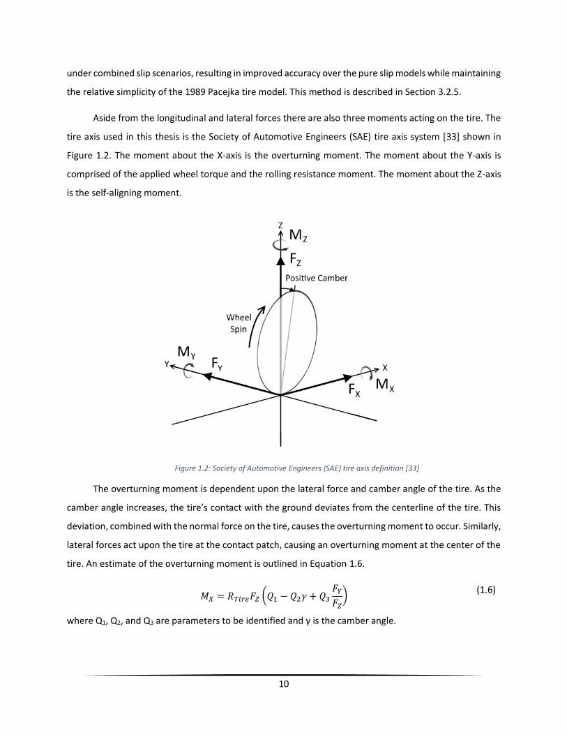
Aside from the longitudinal and lateral forces there are also three moments acting on the tire. The
tire axis used in this thesis is the Society of Automotive Engineers (SAE) tire axis system [33] shown in
Figure 1.2. The moment about the X-axis is the overturning moment. The moment about the Y-axis is
comprised of the applied wheel torque and the rolling resistance moment. The moment about the Z-axis
is the self-aligning moment.
Figure 1.2: Society of Automotive Engineers (SAE) tire axis definition [33]
The overturning moment is dependent upon the lateral force and camber angle of the tire. As the
camber angle increases, the tire’s contact with the ground deviates from the centerline of the tire. This
deviation, combined with the normal force on the tire, causes the overturning moment to occur. Similarly,
lateral forces act upon the tire at the contact patch, causing an overturning moment at the center of the
tire. An estimate of the overturning moment is outlined in Equation 1.6.
𝑀𝑋 = 𝑅𝑇𝑖𝑟𝑒𝐹𝑍 (𝑄1 − 𝑄2𝛾 + 𝑄3
𝐹𝑌
𝐹𝑍
) (1.6)
where Q1, Q2, and Q3 are parameters to be identified and γ is the camber angle.

11
The moment about the Y-axis is primarily comprised of the torque delivered by the engine or motor
through the powertrain. This value is an input to the system; however, in addition to the input torque
there is also a resistive moment caused by the deformation of the tire. This deformation causes the
distribution of the normal load through the contact patch to change, shifting the lumped normal force a
distance of δx from the centerline of the tire. The rolling resistance moment is generally calculated by
multiplying the lumped normal force by δx.
The self-aligning moment is found in a similar manner as the lateral force since it is mainly
dependent upon the tire sideslip. When the tires are turned, the self-aligning moment acts to align the
tire X-axis with the direction of motion. This moment is felt by the driver of the vehicle through the
steering wheel; however autonomous vehicle systems will always define a specific steering angle. Since
this angle is defined as an input to the system, the self-aligning moment will have very little effect on the
dynamics of the vehicle, just applying another load on the steering motor, and can be ignored.

12
2. Data Collection and Experimental Testing
2.1. Data Acquisition System
2.1.1. Vehicle Measurement System
The Vehicle Measurement System, hereafter referred to as the VMS, is a system designed by A&D
Technology [40] that attaches to a vehicle to measure a variety of signals while the vehicle is in motion. It
is designed to capture data through on-road testing. The system is too large and expensive to be used
constantly during normal driving. Instead the system is attached to the vehicle only during specific testing
periods when the vehicle is taken to a dedicated test track or airport runway in order to perform the
desired test maneuvers. The system consists of three main sensor arrays. The test vehicle with the VMS
attached is shown in Figure 2.1.
Figure 2.1: The Moose at the Waterloo Test Track with the VMS

13
The first sensor is the Wheel Force Sensor (WFS) shown in Figure 2.2. The WFS is a custom wheel
hub that consists of an array of strain gauges that measure the forces and moments on the wheel. The
data signals gathered from the WFS are:
− Longitudinal force
− Lateral force
− Vertical forces
− Moment about the longitudinal axis (as defined by SAE tire axis seen in Figure 1.2)
− Moment about the lateral axis (as defined by SAE tire axis)
− Moment about the vertical axis (as defined by SAE tire axis)
− Angular velocity of the wheel
Figure 2.2: Wheel Force Sensor (WFS) attached to custom wheel rim

14
The second sensor is the Wheel Position Sensor (WPS) shown in Figure 2.3. The WPS is a truss
structure with five degrees of freedom that measures the position of the wheel relative to the chassis
through the use of five separate encoders. One section of the truss system is attached to the center of
the wheel hub. The other section is attached to an array of high quality suction cups that are attached to
the vehicle chassis above the wheel. The data signals gathered from the WPS are:
− Longitudinal displacement of the wheel relative to the chassis
− Lateral displacement of the wheel relative to the chassis
− Vertical displacement of the wheel relative to the chassis
− Camber angle of the wheel
− Toe angle of the wheel
Figure 2.3: Wheel Position Sensor (WPS)

15
The last major sensor is the Laser Ground Senor (LGS) shown in Figure 2.4. This sensor array consists
of five laser sensors. Three of these sensors measure the distance from the center of the wheel hub to
the ground. These sensors are also used to account for any changes in tire orientation. This can include
any orientation offset due to installation error. The other two sensors measure the longitudinal and lateral
speed of the vehicle. The data signals gathered from the LGS are:
− Longitudinal speed of the vehicle at the tire
− Lateral speed of the vehicle at the tire
− Effective wheel radius
− Sideslip angle of the tire
Figure 2.4: Laser Ground Sensor (LGS)

16
2.1.2. VBOX 3i
The VBOX 3i by Racelogic [41] is an Inertia Measurement Unit (IMU) coupled with a Global
Positioning System (GPS). The unit is attached to the roof of the vehicle in a known position. The IMU
captures the longitudinal, lateral, and vertical accelerations of the vehicle along with the roll rate, pitch
rate, and yaw rate of the chassis. The GPS captures the location and heading of the vehicle. Coordinate
transformations are necessary to transfer measured values from the sensor location to the center of mass
of the vehicle.
17
2.1.3. Vehicle CAN and Vehicle Control Module
Many of the internal vehicle signals are communicated through the vehicle Controller Area Network
(CAN). Most of these signals are not important for vehicle dynamic modeling and parameter identification;
however, among these signals are the three main inputs to an autonomous vehicle: the steer angle, the
accelerator pedal position, and the brake pedal position. These values were recorded during each
maneuver in order to provide them as the input to the full vehicle dynamic model described in Chapter 3.
18
2.2. Experimental Testing
Many different tests need to be performed in order to get a comprehensive data set for parameter
identification. A few parameters can be developed using longitudinal tests alone, but others require
lateral motion as well. This section provides an overview of the different tests that were designed and
performed to gather a comprehensive data set for each parameter identified in Chapter 3.
2.2.1. Center of Mass Tests
Two different tests can be done to determine the center of mass of the vehicle. The longitudinal
and lateral center of mass locations can be easily identified while the vehicle is static. The height of the
center of mass can be found using either of the two following tests.
The first test is a static test; no vehicle motion is necessary. To perform this test, the vehicle needs
to be placed on a flat surface, and the front wheels need to be lifted off the ground. The front wheels
should be placed on a post with a surface that is parallel to the ground. This causes the vehicle to be
inclined at a set angle. This is an easy test to perform; however, it can take a long time to set up properly
unless a specific test rig is used. In addition, the results may not be accurate if the vehicle angle (θ) is too
small. To get accurate data, the vehicle angle should be around 45 degrees; however, this is generally not
possible since it will likely cause the rear end of the vehicle to hit the ground. A picture of the test setup
is shown in Figure 2.5.
Figure 2.5: Experimental setup for static test to determine the height of the center of mass
19
Point A is at the contact point between the ground and the rear tire. Likewise, point E is the contact
point between the front tire and the raised section of ground. The distance AE is the wheelbase of the
vehicle and the distance DE is the known height that the vehicle was raised above the ground. The weight
at the center of mass is the total weight of the vehicle, calculated by adding all the WFS measurements
together.
The second test that can be completed is a dynamic maneuver. Any maneuver can be used for this
test, so a simple longitudinal test is chosen. A rapid acceleration and braking maneuver is suitable to
determine this parameter. Many different tests were performed with varying degrees of acceleration and
deceleration. In the end it was found that minimizing the rate of change of acceleration provided the best
test data. This is accomplished by performing a test with a single long acceleration event followed by a
large braking event. The vehicle is brought from rest up to a speed of around 100km/h. Once this speed
is reached, the brakes are applied so as to bring the vehicle back to rest. During the deceleration portion
of the test the brake pedal should be kept at a constant position in order to minimize the change in
acceleration of the vehicle. The height of the center of mass is found by solving the moment balance
equation. The forces on each tire are measured using the WFS, and the angular speed of the chassis is
measured using the IMU. The braking region will provide the best test data to use for the parameter
identification due to the relatively constant longitudinal force. Figure 2.6 shows the velocity profile of this
maneuver.
Figure 2.6: Velocity versus time for the center of mass dynamic maneuver

20
2.2.2. Inertia Tests
2.2.2.1. Wheel Inertia Tests
One test is needed to identify the wheel inertia. The vehicle’s driven wheels, the front two wheels,
were lifted off the ground so that they were allowed to roll freely. Once the driven wheels are able to
rotate freely, the vehicle is turned on and an applied driving torque is sent to the wheels, which causes
them to spin. The wheel inertia is found by solving the moment balance equation, requiring torque and
angular acceleration. Both the torque and the angular speed of the wheel are recorded using the WFS.
Shown in Figure 2.7 is the experimentally recorded wheel speed and wheel torque data versus time for a
vehicle driven test.
Figure 2.7: Wheel speed/torque versus time

21
2.2.2.2. Vehicle Inertia Tests
There are four main tests that were performed in order to identify the principal moments of inertia
for the vehicle. One maneuver is a simple longitudinal maneuver. The other three are lateral maneuvers.
The tests have been designed to solve the moment balance equation of the vehicle. Each test was
designed to isolate pitch, roll, and yaw. Due to motion coupling this is not entirely possible; however, it is
possible to minimize the non-desirable angular velocities while maximizing the desired angular velocity.
This produces test data that is biased towards the associated inertial parameter. By combining the data
from all these maneuvers, the principal moments of inertia can be identified more accurately.
The longitudinal maneuver is used to identify the pitch inertia. This maneuver is actually not
required since the pitch inertia can also be identified during the lateral maneuvers; however, this test
leads to better results for the pitch inertia. Similar to the dynamic maneuver seen in Figure 2.6, this
maneuver is an acceleration and braking maneuver. Good results are observed when the pitch rate of the
vehicle is large, which occurs during large acceleration values. Consequentially, the best way to perform
the maneuver is to have a single large acceleration and braking event that causes the vehicle to pitch
rapidly.
The roll and yaw inertias both affect the vehicle’s lateral motion and therefore a lateral maneuver
is required. Three different lateral maneuvers were developed in order to identify the yaw and roll inertia
of the vehicle.
The first maneuver is a high-speed cornering test through a small angle. This maneuver is designed
to cause a relatively low change in yaw angle while simultaneously causing a relatively high change in roll
angle. This allows priority to be placed on roll inertia identification since the yaw and pitch effects are
minimal. The second maneuver is a low-speed cornering test through a large angle. This maneuver causes
a relatively low change in roll angle and a relatively high change in yaw angle. Speeds and steering angles
for the above tests may vary. Multiple runs of this test were completed in order to minimize and maximize
the desired rotational velocities, although this is not strictly necessary in order to identify the principal
moments of inertia. The last maneuver is a basic sinusoidal steering maneuver where the steering wheel
angle follows a sinusoidal curve that results in the vehicle swerving back and forth. In this test, the vehicle
is put on cruise control in order to minimize the pitch of the vehicle. Large variations in yaw angle and roll
angle are encountered in this maneuver, which can then be used to validate any results obtained from
the previous two tests.
22
2.2.3. Coefficient of Drag and Rolling Resistance Tests
One test is needed to determine the coefficient of drag and the rolling resistance of the wheels;
however, multiple runs of the test are required. The test is purely longitudinal and requires a large straight
flat runway to allow the vehicle to coast down without introducing any lateral motion. As such it was
performed at the Waterloo International Airport, seen in Figure 2.8.
Figure 2.8: Lincoln MKZ at Waterloo International Airport for drag testing
The vehicle is brought up to a speed of 130 km/h and then switched into neutral mode and allowed
to coast down to a speed of 10 km/h. The vehicle is switched into neutral to avoid any regenerative braking
effect, along with other potential resistive effects beyond the resistive forces caused by drag and rolling
resistance, such as any powertrain inertial effects. Note that associated friction forces of the drive line up
to the gearbox are lumped with the rolling resistance of the tires since it is not possible to isolate the
wheels further without using a dedicated test rig.
Data was only used while the vehicle was in the neutral gear. Speeds higher than 120 km/h proved
to provide more erroneous data points due to many of the simplifying assumptions that are described in
Section 3.2.3. This test was performed both up and down the runway in order to minimize any effect of
road slope, which would add an additional gravitational resistive force on the vehicle. The wind speed and
direction were recorded using the weather station in the airport’s control tower. Due to the sensitive
nature of this test, especially with many rapidly changing variables such as wind speed and heading,
multiple runs are needed in order to acquire a sufficiently rich data set.

23
2.2.4. Suspension Tests
Initially a 4-post test was performed to determine the vehicle parameters. As described in Section
1.3.1, 4-post testing involves placing the test vehicle on four individually actuated posts as seen in Figure
2.9. The vehicle should be in park to ensure that the vehicle will not roll off the posts during testing. Two
accelerometers are placed above each post on both the sprung and unsprung mass (chassis and tires).
The testing consists of a sinusoidal frequency sweep with a constant maximum velocity through all the
frequencies. The test lasts for 30 seconds, starting at 1Hz, increasing to 10Hz at 15 seconds. Higher
frequency data is ignored when identifying suspension parameters in order to minimize the effects of high
frequency noise and other behaviours that are difficult to characterize. In addition, the natural frequency
of a well-tuned vehicle suspension is generally under 10Hz [42].
Figure 2.9: Lincoln MKZ on 4-post test rig
As mentioned earlier, the Moose has a semi-active suspension system, meaning that the damping
coefficient is not a constant value, but actually changes based on the motion of the vehicle. Since the
semi-active suspension system is not active when the vehicle is at rest, a set of tests had to be devised in
order to get similar data while the vehicle was in motion. Consequentially the following set of tests can
be used in lieu of a 4-post-test rig. Note that the control logic for the semi-active system is not known,
and as such many additional tests were performed in order to determine what parameters influenced the
damping coefficient to change. Many of these tests turned out to be unnecessary due to the simplicity of
24
the control logic described in Section 3.2.4. Since they are not necessary they are not described in this
thesis.
The first on-road test performed for determining suspension parameters was a simple longitudinal
acceleration and braking maneuver. Unlike other acceleration and braking maneuvers that consist of a
single acceleration and braking event, this maneuver consists of multiple smaller acceleration and braking
events. These events should vary in length and magnitude. The goal is to cause the vehicle to pitch at
different rates to determine if pitch rate has any effect on the semi-active control system.
The second on-road test performed for determining suspension parameters was a rapid swerving
maneuver. Like the above test, the goal of this test is to cause the vehicle to roll. This test is similar to the
final test performed in Section 2.2.2.2. The vehicle is brought up to a speed of 60, 80, and 100km/h and
put on cruise control in order to minimize any longitudinal acceleration and pitch motion. The vehicle is
then rapidly swerved from side to side. For each speed, two different tests are performed. One test
involves quickly turning the steering wheel 30, 20, and 10 degrees (respectively for 60, 80, and 100km/h
speeds) to either side. The other test involves turning the steering wheel 90, 60, and 30 degrees to either
side at a much slower rate. The rates of change may need to be adjusted for different vehicles in order to
get suitable amounts of roll and suspension travel.
Suspension travel is measured using the WPS. It is worth noting that most suspension systems do
not travel in a straight vertical direction but at some angle. As the suspension compresses and
decompresses there is also some change in camber angle, along with potential changes in longitudinal
and lateral positions. To account for these additional changes in suspension travel, another test is needed.
The last test is a static test that is used for identifying the specific trajectory followed by the wheel
center as the suspension system is compressed and decompressed. This is done by using the WPS to
record the position of the wheel relative to the chassis while compressing and decompressing the
suspension system in a controlled environment. This can be done through use of a simple car jack although
better results are achieved when using a full vehicle lift. If using a vehicle lift, once the vehicle is fully
raised off the ground, each individual wheel can be raised and lowered using a separate jack in order to
measure the specific trajectory that the wheel travels when the suspension is compressed or
decompressed. By following this procedure all dynamic effects are ignored and the kinematic motion of
the center of the wheel is identified.

25
2.2.5. Tire Tests
Three different sets of maneuvers were developed for determining the Pacejka parameters for the
vehicle’s tires. One set of tests focuses on the pure longitudinal slip model. The next set focuses on the
pure lateral slip model. The last set focuses on the combined slip model. For more details on the specifics
of these models refer to Section 3.2.5. All testing was completed on dry pavement during warm summer
months.
To get data for the pure longitudinal slip model, a rapid acceleration and braking test is performed.
The vehicle is accelerated quickly from rest to a speed of around 100km/h, after which the brakes are
applied, returning to rest as quickly as possible. A lower top speed can be used if necessary. The most
important part of this test is the quick transients that will excite large longitudinal slip, filling in most of
the nonlinear data regions. This single test is able to provide sufficient data for the pure longitudinal slip
Pacejka model.
As opposed to the single test needed for the longitudinal model, three different tests are performed
to obtain a sufficiently rich dataset for the pure lateral slip model. First, a steady state cornering test is
performed. This test involves driving in a circle with a constant radius at a constant speed. This test is
performed according to ISO standards [43] with a radius of 15m, 20m, and 25m. The second test is a
double lane change maneuver. In this test, the vehicle travels at a constant speed through a typical double
lane change motion. This test is also performed according to ISO standards [44-45] at speeds of 60km/h,
80km/h, and 100km/h. The last test is a step steer test. This test involves traveling in a straight line at a
constant speed and then suddenly applying a large steer input. This is also done according to ISO standards
[46] at speeds of 50km/h, 60km/h, and 70km/h with an approximate 120deg, 90deg, and 60deg steer
angle input respectively.
It can be difficult to obtain data for pure longitudinal or pure lateral slip models using on-road data.
This is simply because of the lack of control available during the road tests. For the above tests, the
gathered data contains both pure slip and combined slip data points. For the pure longitudinal slip test it
is relatively easy to ensure a small sideslip angle by keeping the steering wheel straight. Throughout this
test there is a small constant sideslip angle caused from the toe angle, necessary for vehicle controllability;
however any data points with larger sideslip values are ignored for the pure slip analysis. Likewise, for the
pure lateral slip tests, any data points with large longitudinal slip are disregarded during the analysis.

26
Maintaining small longitudinal slip values throughout the lateral tests is more difficult, but with the large
variety of tests performed, a comprehensive data set is gathered.
For the combined slip Pacejka model, two tests are used to obtain the necessary data. First, a
modified step steer test is performed. The only difference from the above test procedure is that after the
steering angle is applied, a large braking force is also applied. This results in data that has both a large
longitudinal slip and a large side-slip angle. This test is only able to gather data for the negative longitudinal
slip (braking) region since it is difficult to achieve large positive longitudinal slip during this maneuver
unless the vehicle has a powerful engine.
The second test that is performed is the grand sweep maneuver. In this test, the steering wheel
angle changes at a constant rate in either the clockwise or counter-clockwise direction according to the
following criteria. The speed of the vehicle is not to exceed 70km/h and not to fall below 30km/h. While
increasing the steer angle in either direction past the neutral straight wheel state (a steering angle of zero
degrees) the brakes are to be applied. The braking should be applied so as to slow down the vehicle from
the approximate speeds of 70km/h to 30km/h by the time the steering wheel angle rotates a full 360
degrees. After the vehicle slows down, the steer angle is moved back to the neutral straight wheel state
at the same rate of change used previously. During this time the accelerator pedal should be applied. The
acceleration should be applied so as to speed up the vehicle from the approximate speeds of 30km/h to
70km/h by the time the steering wheel angle returns to zero degrees – the neutral straight wheel state.
Once the steering angle is back to zero degrees the wheel should continue to rotate in the same direction
– so as to turn the vehicle in the other direction – with the above criteria in mind. This process is repeated
a total of ten times. Ultimately this maneuver results in the vehicle traveling in a rough figure eight pattern
as seen in Figure 2.10. Similar to the previous test, it is more difficult to excite large positive longitudinal
slip than it is to excite large negative longitudinal slip; a powerful engine would be needed in order to
excite this region.

27
Figure 2.10: Sample vehicle trajectory of the grand sweep maneuver
Many different tests had to be altered and repeated to improve data quality and repeatability. All
the tests detailed above are the final versions, easily repeatable with the exception of the grand sweep
maneuver. All the pure lateral slip tests are according to ISO standards and the desired trajectories were
outlined with low profile traffic pylons to ensure the tests adhered to the standards. The pure longitudinal
test is simple and repeatable. The only test that is not easily repeatable is the grand sweep maneuver;
however, since the test involves multiple runs it is easy enough to duplicate the gathered data even
though the runs may be slightly different.
28
3. Vehicle Dynamic Modeling and Parameter
Identification
3.1. Modelling
The vehicle that is modelled in this thesis is the Moose, a 2015 Hybrid Electric Lincoln MKZ. The
vehicle has been turned into a drive-by-wire vehicle by AutonomouStuff [48]. This means that the steering
wheel angle, accelerator pedal position, and brake pedal position can be changed through an electrical
signal. Through this process the Antilock Brake System (ABS), Traction Control System (TCS), and Electronic
Stability Control (ESC) were disabled. Throughout all the testing detailed in Section 2.2 these systems were
never encountered. As such they are not considered when modelling the vehicle. There has been previous
work using the VMS for vehicle parameter identification and modelling; however, it has been limited to
longitudinal dynamics [49-50].
The vehicle is modelled using MapleSim 2017.3, a software developed by Maplesoft [51] for
dynamic modeling and simulation. One advantage of this software is the use of symbolics and acausal
modelling, which leads to faster computation times than conventional numeric software such as Matlab.
The vehicle is modelled as a 14-degree of freedom rigid body model. The chassis is considered to be one
rigid body with a full 6 degrees of freedom. Each tire has one degree of freedom allowing the wheel to
spin. The front two wheels are also allowed to rotate about the vertical axis in order to model the steering
of the vehicle; however these values are specified as an input steer value and therefore are not additional
degrees of freedom. The last four degrees of freedom are modelled in the suspension system of the
vehicle, allowing the suspension to compress and decompress.
The model has five inputs and forty-three outputs. A summary of the inputs and outputs is shown
in Table 3.1. The outputs are the states of the vehicle and tires. Fifteen of these outputs are the states of
the chassis. There are three outputs for each of the position, velocity, acceleration, orientation, rate of
change of orientation of the chassis. There are seven outputs for the states of each wheel. There are three
outputs for the position and orientation of each wheel, and another output for the rotational speed of
each wheel. Since there are four wheels, there are a total of twenty-eight outputs for all wheels together.

29
It is worth noting that many of the outputs are not unique. Some of these values are simply outputted for
convenience when using the model in a simulation environment. Many of the other values represent
sensor readings that are captured for validation. These values can also be used in the simulation
environment to mimic the values that would be captured from real life sensors.
The inputs to the model are the steering wheel angle and each of the four wheel torques. Another
model has been developed by Bryce Hosking [52], which consists of the vehicle’s powertrain and braking
model. The powertrain model has two inputs and four outputs. The two inputs are the accelerator and
brake pedal positions, and the four outputs are the four wheel torques. That model is designed to be used
as a precursor to the model developed in this thesis, reducing the inputs to the steering wheel angle,
accelerator pedal position, and brake pedal position. These are the inputs needed for an autonomous
vehicle. For the development and validation of the vehicle dynamic model presented in this thesis, the
powertrain model is not considered.
Name Description
Output (3) Chassis Position Global position of chassis (PX, PY, PZ)
Output (3) Chassis Velocity Local velocity of chassis (VLONG, VLAT, VZ)
Output (3) Chassis Acceleration Local acceleration of chassis (ALONG, ALAT, AZ)
Output (3) Chassis Orientation Global orientation of chassis (𝑃𝑖𝑡𝑐ℎ, 𝑅𝑜𝑙𝑙, 𝑌𝑎𝑤)
Output (3) Chassis Angular Velocity Local angular velocity of chassis (𝑃𝑖𝑡𝑐ℎ̇ , 𝑅𝑜𝑙𝑙̇ , 𝑌𝑎𝑤̇ )
Output (12) Wheel Position Local position of each wheel (PX_FL, PY_FL, PZ_FL, PX_FR, PY_FR,
PZ_FR, PX_RL, PY_RL, PZ_RL¸ PX_RR, PY_RR, PZ_RR)
Output (12) Wheel Orientation Local orientation of each wheel (θFL, φFL, βFL, θFR, φFR, βFR,
θRL, φRL, βRL¸ θRR, φRR, βRR)
Output (4) Wheel Spin Rate Spin rate of each wheel (𝜔𝐹𝐿, 𝜔𝐹𝑅, 𝜔𝑅𝐿, 𝜔𝑅𝑅)
Input (1) Steering Wheel Angle Angle of the steering wheel (δ)
Input (4) Wheel Torque Torque at each wheel (TFL, TFR, TRL, TRR)
Table 3.1: Summary of the model inputs and outputs
30
3.2. Parameter Identification Using Simple Models
All parameters in this section are identified using simple models. This reduces the complexity of the
system and allows the parameters to be identified easier; however, it also reduces the accuracy of the
determined parameters. Once the rough approximation of all the parameters are identified, they are
refined using the high-fidelity model as described in Section 3.3.
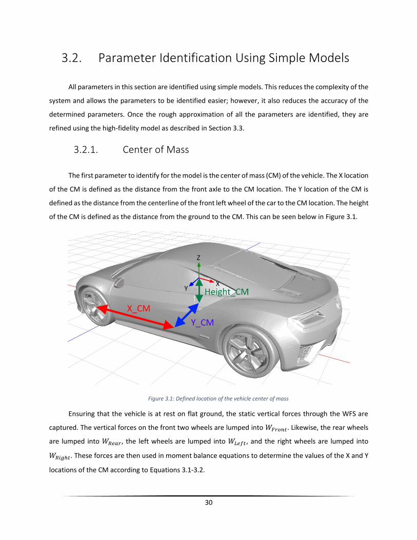
3.2.1. Center of Mass
The first parameter to identify for the model is the center of mass (CM) of the vehicle. The X location
of the CM is defined as the distance from the front axle to the CM location. The Y location of the CM is
defined as the distance from the centerline of the front left wheel of the car to the CM location. The height
of the CM is defined as the distance from the ground to the CM. This can be seen below in Figure 3.1.
Figure 3.1: Defined location of the vehicle center of mass
Ensuring that the vehicle is at rest on flat ground, the static vertical forces through the WFS are
captured. The vertical forces on the front two wheels are lumped into 𝑊𝐹𝑟𝑜𝑛𝑡. Likewise, the rear wheels
are lumped into 𝑊𝑅𝑒𝑎𝑟, the left wheels are lumped into 𝑊𝐿𝑒𝑓𝑡, and the right wheels are lumped into
𝑊𝑅𝑖𝑔ℎ𝑡. These forces are then used in moment balance equations to determine the values of the X and Y
locations of the CM according to Equations 3.1-3.2.
31
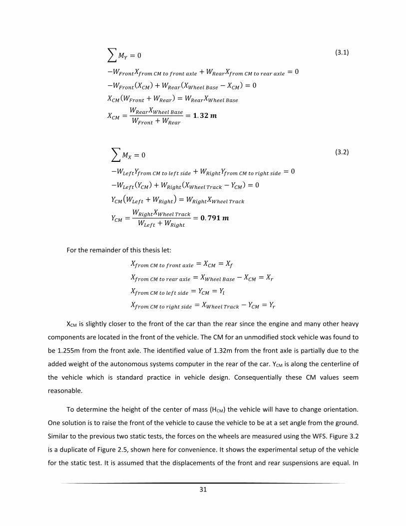
∑ 𝑀𝑌 = 0
−𝑊𝐹𝑟𝑜𝑛𝑡𝑋𝑓𝑟𝑜𝑚 𝐶𝑀 𝑡𝑜 𝑓𝑟𝑜𝑛𝑡 𝑎𝑥𝑙𝑒 + 𝑊𝑅𝑒𝑎𝑟𝑋𝑓𝑟𝑜𝑚 𝐶𝑀 𝑡𝑜 𝑟𝑒𝑎𝑟 𝑎𝑥𝑙𝑒 = 0
−𝑊𝐹𝑟𝑜𝑛𝑡(𝑋𝐶𝑀) + 𝑊𝑅𝑒𝑎𝑟(𝑋𝑊ℎ𝑒𝑒𝑙 𝐵𝑎𝑠𝑒 − 𝑋𝐶𝑀) = 0
𝑋𝐶𝑀(𝑊𝐹𝑟𝑜𝑛𝑡 + 𝑊𝑅𝑒𝑎𝑟) = 𝑊𝑅𝑒𝑎𝑟𝑋𝑊ℎ𝑒𝑒𝑙 𝐵𝑎𝑠𝑒
𝑋𝐶𝑀 =𝑊𝑅𝑒𝑎𝑟𝑋𝑊ℎ𝑒𝑒𝑙 𝐵𝑎𝑠𝑒
𝑊𝐹𝑟𝑜𝑛𝑡 + 𝑊𝑅𝑒𝑎𝑟= 𝟏. 𝟑𝟐 𝒎
(3.1)
∑ 𝑀𝑋 = 0
−𝑊𝐿𝑒𝑓𝑡𝑌𝑓𝑟𝑜𝑚 𝐶𝑀 𝑡𝑜 𝑙𝑒𝑓𝑡 𝑠𝑖𝑑𝑒 + 𝑊𝑅𝑖𝑔ℎ𝑡𝑌𝑓𝑟𝑜𝑚 𝐶𝑀 𝑡𝑜 𝑟𝑖𝑔ℎ𝑡 𝑠𝑖𝑑𝑒 = 0
−𝑊𝐿𝑒𝑓𝑡(𝑌𝐶𝑀) + 𝑊𝑅𝑖𝑔ℎ𝑡(𝑋𝑊ℎ𝑒𝑒𝑙 𝑇𝑟𝑎𝑐𝑘 − 𝑌𝐶𝑀) = 0
𝑌𝐶𝑀(𝑊𝐿𝑒𝑓𝑡 + 𝑊𝑅𝑖𝑔ℎ𝑡) = 𝑊𝑅𝑖𝑔ℎ𝑡𝑋𝑊ℎ𝑒𝑒𝑙 𝑇𝑟𝑎𝑐𝑘
𝑌𝐶𝑀 =𝑊𝑅𝑖𝑔ℎ𝑡𝑋𝑊ℎ𝑒𝑒𝑙 𝑇𝑟𝑎𝑐𝑘
𝑊𝐿𝑒𝑓𝑡 + 𝑊𝑅𝑖𝑔ℎ𝑡= 𝟎. 𝟕𝟗𝟏 𝒎
(3.2)
For the remainder of this thesis let:
𝑋𝑓𝑟𝑜𝑚 𝐶𝑀 𝑡𝑜 𝑓𝑟𝑜𝑛𝑡 𝑎𝑥𝑙𝑒 = 𝑋𝐶𝑀 = 𝑋𝑓
𝑋𝑓𝑟𝑜𝑚 𝐶𝑀 𝑡𝑜 𝑟𝑒𝑎𝑟 𝑎𝑥𝑙𝑒 = 𝑋𝑊ℎ𝑒𝑒𝑙 𝐵𝑎𝑠𝑒 − 𝑋𝐶𝑀 = 𝑋𝑟
𝑋𝑓𝑟𝑜𝑚 𝐶𝑀 𝑡𝑜 𝑙𝑒𝑓𝑡 𝑠𝑖𝑑𝑒 = 𝑌𝐶𝑀 = 𝑌𝑙
𝑋𝑓𝑟𝑜𝑚 𝐶𝑀 𝑡𝑜 𝑟𝑖𝑔ℎ𝑡 𝑠𝑖𝑑𝑒 = 𝑋𝑊ℎ𝑒𝑒𝑙 𝑇𝑟𝑎𝑐𝑘 − 𝑌𝐶𝑀 = 𝑌𝑟
XCM is slightly closer to the front of the car than the rear since the engine and many other heavy
components are located in the front of the vehicle. The CM for an unmodified stock vehicle was found to
be 1.255m from the front axle. The identified value of 1.32m from the front axle is partially due to the
added weight of the autonomous systems computer in the rear of the car. YCM is along the centerline of
the vehicle which is standard practice in vehicle design. Consequentially these CM values seem
reasonable.
To determine the height of the center of mass (HCM) the vehicle will have to change orientation.
One solution is to raise the front of the vehicle to cause the vehicle to be at a set angle from the ground.
Similar to the previous two static tests, the forces on the wheels are measured using the WFS. Figure 3.2
is a duplicate of Figure 2.5, shown here for convenience. It shows the experimental setup of the vehicle
for the static test. It is assumed that the displacements of the front and rear suspensions are equal. In
32
reality this is not the case; however the suspension displacement difference is small enough to cause the
error to remain small.
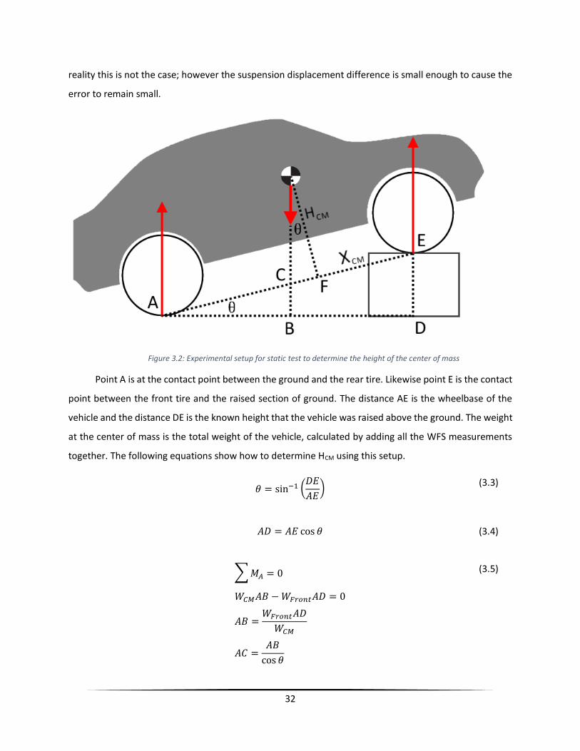
Figure 3.2: Experimental setup for static test to determine the height of the center of mass
Point A is at the contact point between the ground and the rear tire. Likewise point E is the contact
point between the front tire and the raised section of ground. The distance AE is the wheelbase of the
vehicle and the distance DE is the known height that the vehicle was raised above the ground. The weight
at the center of mass is the total weight of the vehicle, calculated by adding all the WFS measurements
together. The following equations show how to determine HCM using this setup.
𝜃 = sin−1 (
𝐷𝐸
𝐴𝐸)
(3.3)
𝐴𝐷 = 𝐴𝐸 cos 𝜃
(3.4)
∑ 𝑀𝐴 = 0
𝑊𝐶𝑀𝐴𝐵 − 𝑊𝐹𝑟𝑜𝑛𝑡𝐴𝐷 = 0
𝐴𝐵 =𝑊𝐹𝑟𝑜𝑛𝑡𝐴𝐷
𝑊𝐶𝑀
𝐴𝐶 =𝐴𝐵
cos 𝜃
(3.5)
33
Using the above information, the small distance CF can be determined and used to find HCM.
𝐶𝐹 = 𝐴𝐸 − 𝐴𝐶 − 𝑋𝐶𝑀
𝐻𝐶𝑀 =𝐶𝐹
tan 𝜃= 𝟎. 𝟓𝟑𝟒𝒎
(3.6)
This value for HCM seems reasonable based on known values of other similar vehicles [53]. To
minimize error, the vehicle should be lifted to create an angle (θ) of around 45 degrees. This helps
minimize the error due to the trigonometric functions; however, it can be more difficult to set up a test
rig in this manner. Multiple tests can also be performed at different angles to reduce the error. This is
similar to the tests performed on a dynamic test platform as outlined in Section 1.3.1.
In addition to the above tests, the vehicle was tested on a 4-post test rig as detailed in Section 2.2.4.
The 4-post test rig can act like a dynamic test platform. By pitching and rolling the vehicle the center of
mass can be identified. Shown below, in Table 3.2, is a comparison between the results from the 4-post
testing software and the results calculated above using the VMS.
Center of Mass [m] 4-Post Testing VMS Testing (Static) % Error
XCM 1.27 1.32 3.8 %
YCM 0.759 0.791 4.0 %
HCM 0.556 0.534 4.1 %
Table 3.2: CM location comparison between 4-post testing and VMS testing
There are a few reasons for the small differences between the calculated CM from 4-post testing
and the calculated CM from the static equilibrium model. First, there was a simulated driver weight during
the 4-post testing; however, during the static equilibrium calculations there was both a simulated driver
and a simulated passenger weight in the vehicle. This extra weight would increase the YCM of the vehicle.
During the 4-post testing some of the equipment from the rear of the vehicle was also removed to be
repaired and upgraded. This is the major reason for the differences seen in Table 3.2. It is common for the
equipment on the vehicle to be added, removed, or moved around. Due to this fact, the above procedure
is repeated at the beginning of each round of testing to identify the current CM location. The only
exception is the test for determining the height of the center of mass. Instead of repeating the above
static test, a dynamic test is performed since the inertia of the vehicle known (and reidentified for each
maneuver) and the static test can be lengthy.
34
The dynamic test performed is outlined in Section 2.2.1. Both the accelerating and braking regions
can be used to determine HCM; however, the braking region generally has a more consistent acceleration,
and consequentially this range of test data is used. The same moment balance equation used for XCM and
YCM cannot be used to determine HCM since the vehicle is not at rest. The vehicle inertia is identified in
Section 3.2.2.2 and is used here to calculate HCM as shown in Equation 3.7. It is assumed that the transverse
effects are small and therefore ignored. See Section 3.2.2.2 for more details.
∑ 𝑀𝑌 = 𝐼𝑌�̇�𝑌
𝑊𝑅𝑒𝑎𝑟𝑋𝑟−𝑊𝐹𝑟𝑜𝑛𝑡𝑋𝑓 − 𝐹𝐿𝑜𝑛𝑔𝑖𝑡𝑢𝑑𝑖𝑛𝑎𝑙𝐻𝐶𝑀 = 𝐼𝑌�̇�𝑌
(3.7)
This equation is used to solve for HCM. Generally the braking region provides better results than the
accelerating region due to a more constant longitudinal force. An example of the calculated HCM versus
time for the dynamic test outlined in Section 2.2.1 can be seen below in Figure 3.3. The results shown are
from the most recent set of test data (June 2018). The optimal least square value during the duration of
the braking region of the maneuver is used as the height of the center of mass. This value is shown as the
constant line in Figure 3.3.
Figure 3.3: HCM versus time for dynamic maneuver
From the same set of data, the XCM and YCM have also been calculated. A comparison of CM locations
by date is shown in Table 3.3. XCM and YCM were calculated in the same method described, while HCM was
calculated using the dynamic test method instead of the static lift calculations.
35
Center of Mass [m] VMS Testing (Static)
April 2017
VMS Testing (Dynamic)
August 2017
VMS Testing (Dynamic)
June 2018
XCM 1.32 1.33 1.39
YCM 0.791 0.811 0.865
HCM 0.534 0.531 0.566
Table 3.3: Comparison of CM locations over time
It can be seen that the CM location changes from test to test. For the remainder of this thesis it is
assumed that the CM values used are the values calculated for that set of testing. It should be noted that
as equipment (such as LIDAR, cameras, computers, and supporting mechanical framework for the
aforementioned equipment) has been added to the vehicle, the Y location of the center of mass has
deviated from the center line of the vehicle. This can have negative effects on vehicle handling.
In the future it is assumed that no more major changes will be done on the vehicle. At that point it
will be possible to recalculate the CM of the vehicle and assume it will remain constant for all further
testing, both for modelling and any controller development.
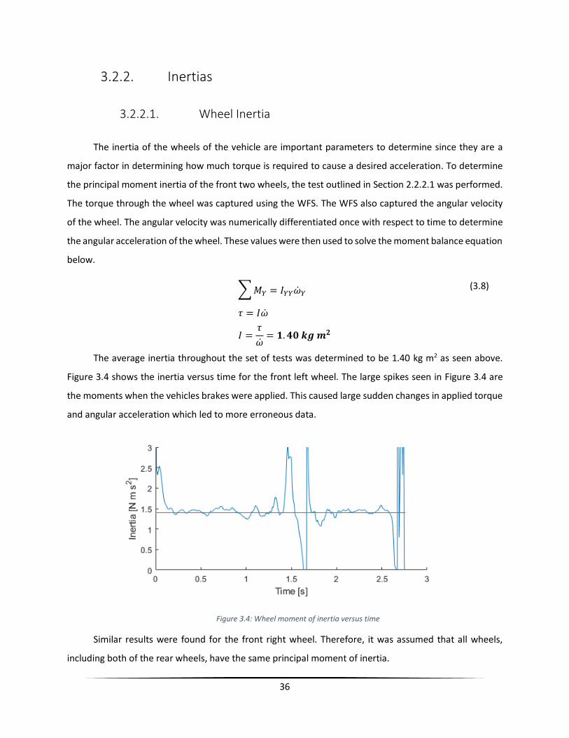
36
3.2.2. Inertias
3.2.2.1. Wheel Inertia
The inertia of the wheels of the vehicle are important parameters to determine since they are a
major factor in determining how much torque is required to cause a desired acceleration. To determine
the principal moment inertia of the front two wheels, the test outlined in Section 2.2.2.1 was performed.
The torque through the wheel was captured using the WFS. The WFS also captured the angular velocity
of the wheel. The angular velocity was numerically differentiated once with respect to time to determine
the angular acceleration of the wheel. These values were then used to solve the moment balance equation
below.
∑ 𝑀𝑌 = 𝐼𝑌𝑌�̇�𝑌
𝜏 = 𝐼�̇�
𝐼 =𝜏
�̇�= 𝟏. 𝟒𝟎 𝒌𝒈 𝒎𝟐
(3.8)
The average inertia throughout the set of tests was determined to be 1.40 kg m2 as seen above.
Figure 3.4 shows the inertia versus time for the front left wheel. The large spikes seen in Figure 3.4 are
the moments when the vehicles brakes were applied. This caused large sudden changes in applied torque
and angular acceleration which led to more erroneous data.
Figure 3.4: Wheel moment of inertia versus time
Similar results were found for the front right wheel. Therefore, it was assumed that all wheels,
including both of the rear wheels, have the same principal moment of inertia.

37
3.2.2.2. Vehicle Inertia
The inertia of the vehicle is an important parameter to identify; however, as noted in Section 3.2.1,
since the vehicle is modified constantly, the inertia parameters will change slightly between each testing
session. Like the center of mass, the vehicle inertia must be identified at the beginning of each round of
testing.
The pitch inertia is isolated since a maneuver can be performed on the vehicle that will excite very
small amounts of roll and yaw angles. By keeping these angles small, they can be effectively ignored. A
free body diagram of the vehicle is shown in Figure 3.5.
∑ 𝑀𝑌 = 𝐼𝑌𝑌�̇�𝑌
𝐼𝑌𝑌 =𝑊𝑅𝑒𝑎𝑟𝑋𝑟−𝑊𝐹𝑟𝑜𝑛𝑡𝑋𝑓 − 𝐹𝐿𝑜𝑛𝑔𝑖𝑡𝑢𝑑𝑖𝑛𝑎𝑙𝐻𝐶𝑀
�̇�𝑌= 𝟑𝟕𝟎𝟓 𝒌𝒈 𝒎𝟐
(3.9)
Figure 3.5: Free body diagram of the vehicle during a longitudinal maneuver
38
To determine the other moments of inertia of the vehicle, a full moment balance equation is
needed. This is since both vehicle yaw and roll are related to the lateral movement of the vehicle, and as
such they are difficult to isolate.
∑ 𝑀𝑋 = 𝐼𝑋𝑋�̇�𝑋 − (𝐼𝑌𝑌 − 𝐼𝑍𝑍)𝜔𝑌𝜔𝑍 (3.10)
∑ 𝑀𝑍 = 𝐼𝑍𝑍�̇�𝑍 − (𝐼𝑋𝑋 − 𝐼𝑌𝑌)𝜔𝑋𝜔𝑌
(3.11)
Since small amounts of pitch are also encountered in this maneuver, the pitch inertia can be
identified again and compared to the previous results
∑ 𝑀𝑌 = 𝐼𝑌𝑌�̇�𝑌 − (𝐼𝑍𝑍 − 𝐼𝑋𝑋)𝜔𝑍𝜔𝑋
(3.12)
A non-linear least squares optimization routine was run in order to identify the three principal
moments of inertia. The results are as follows:
𝐼𝑋𝑋 = 𝟏𝟕𝟖𝟔 𝒌𝒈 𝒎𝟐
𝐼𝑌𝑌 = 𝟑𝟕𝟏𝟐 𝒌𝒈 𝒎𝟐
𝐼𝑍𝑍 = 𝟒𝟏𝟗𝟕 𝒌𝒈 𝒎𝟐
For future testing sessions, Equations 3.10-3.12 are re-optimized to identify the updated moments
of inertia for the vehicle. Generally the changes are minor.
During the above calculations all the products of inertia are ignored as they are relatively small. This
is because the defined vehicle fixed axis is close to the principal direction due to the symmetry of the
vehicle. The vehicle is not perfectly symmetrical, which causes some transverse effects to be seen.
Equations 3.13-3.15 show the results including the products of inertia.

39
∑ 𝑀𝑋 = 𝐼𝑋𝑋�̇�𝑋 − (𝐼𝑌𝑌 − 𝐼𝑍𝑍)𝜔𝑌𝜔𝑍 − 𝐼𝑋𝑌(�̇�𝑌 − 𝜔𝑍𝜔𝑋) − 𝐼𝑌𝑍(𝜔𝑌2 − 𝜔𝑍
2)
− 𝐼𝑍𝑋(�̇�𝑍 − 𝜔𝑋𝜔𝑌)
(3.13)
∑ 𝑀𝑌 = 𝐼𝑌𝑌�̇�𝑌 − (𝐼𝑍𝑍 − 𝐼𝑋𝑋)𝜔𝑍𝜔𝑋 − 𝐼𝑌𝑍(�̇�𝑍 − 𝜔𝑋𝜔𝑌) − 𝐼𝑍𝑋(𝜔𝑍2 − 𝜔𝑋
2)
− 𝐼𝑋𝑌(�̇�𝑋 − 𝜔𝑌𝜔𝑍)
(3.14)
∑ 𝑀𝑍 = 𝐼𝑍𝑍�̇�𝑍 − (𝐼𝑋𝑋 − 𝐼𝑌𝑌)𝜔𝑋𝜔𝑌 − 𝐼𝑍𝑋(�̇�𝑋 − 𝜔𝑌𝜔𝑍) − 𝐼𝑋𝑌(𝜔𝑋2 − 𝜔𝑌
2)
− 𝐼𝑌𝑍(�̇�𝑌 − 𝜔𝑍𝜔𝑋)
(3.15)
Another non-linear least squares optimization routing was run to identify all the inertial
parameters. The results are as follows:
𝐼𝑋𝑋 = 𝟏𝟖𝟔𝟏 𝒌𝒈 𝒎𝟐
𝐼𝑌𝑌 = 𝟑𝟔𝟗𝟓 𝒌𝒈 𝒎𝟐
𝐼𝑍𝑍 = 𝟒𝟐𝟖𝟏 𝒌𝒈 𝒎𝟐
𝐼𝑋𝑌 = 𝟐𝟒 𝒌𝒈 𝒎𝟐
𝐼𝑌𝑍 = 𝟑𝟔 𝒌𝒈 𝒎𝟐
𝐼𝑍𝑋 = 𝟏𝟏𝟐 𝒌𝒈 𝒎𝟐
As can be seen the products of Inertias – 𝐼𝑋𝑌, 𝐼𝑌𝑍, 𝐼𝑍𝑋 – are small and consequentially ignored in
order to simplify the model and subsequent equations. If any product of inertia were to be included in the
model then it would be IZX. This value is the largest of the three values and occurs due to the relationship
that both the roll and yaw motions have with the lateral movement of the vehicle.
40
3.2.3. Coefficient of Drag and Rolling Resistance
The largest resistive forces acting on the vehicle are the drag force and rolling resistance force. The
rolling resistance force calculated in this section is only used with the linear tire model. This is because
the linear tire model used in this thesis does not account for the rolling resistance moment unlike the
Pacejka tire model developed in Section 3.2.5. That section also identifies an updated rolling resistance
moment for use in the Pacejka tire model. For the linear tire model, it is sufficient to simplify the rolling
resistance coefficient by considering it as a constant value. In reality the rolling resistance is not constant;
however, for speeds below 70km/h the change in rolling resistance is insignificant [18]. Equation 3.16
shows the equation used for calculating the drag force.
𝐹𝐷𝑟𝑎𝑔 = 12⁄ 𝜌𝐶𝑑𝐴𝐹(𝑉 + 𝑉𝑤)2
(3.16)
where 𝜌 is the density of air (1.2 kg/m3), 𝐶𝑑 is the aerodynamic drag coefficient (to be determined), 𝐴𝐹 is
the frontal area of the vehicle, 𝑉 is the longitudinal speed of the CM, and 𝑉𝑤 is the headwind speed.
The speed of the wind and the wind heading are provided by the weather station at the airport.
These values can be used together to determine the headwind velocity. During testing there was no
headwind, only a crosswind. As such, only the measured velocity of the CM was used in Equation 3.16.
An approximation of the frontal area of the vehicle is calculated by processing a picture of the front
of the vehicle. Figure 3.6 is the image that was captured. This image was used to generate the binary
image seen in Figure 3.7.

41
Figure 3.6: Front Profile of the Lincoln MKZ
Figure 3.7: Frontal area of the Lincoln MKZ
Figure 3.7 is used to calculate the frontal area of the vehicle. This is accomplished by trimming the
image so that the real life height and width of the picture is known. The width of the image is trimmed so
that the edges of the image line up with the far edges of the side mirrors of the vehicle since the distance
between the side mirrors is a known value. The height of the image is initially trimmed to line up with the
bottom of the tires and the top of the roof of the vehicle since the height of the vehicle is also a known
value. Unfortunately, due to all the equipment on top of the vehicle, the height of the full image is not
known. To set the image height to a known value, the image is first trimmed down to the known height –
42
from the bottom of the tires to the roof of the car – and then the image height is multiplied by 1.5 to
increase the height of the image by a known value.
It is worth noting that there are some slight differences between Figure 3.6 and Figure 3.7. Between
the time when Figure 3.6 was taken and the time drag testing occurred there were some modifications
done to the equipment on the roof of the vehicle. This can be seen by comparing Figure 3.6 with Figure
2.8. To adjust for this change some additional processing was completed. Even with the changes to the
roof equipment, Figure 3.7 is still missing all the frontal area generated by the addition of the VMS. During
future testing, the VMS will not be attached, so the frontal area shown Figure 3.7 in will be accurate.
Since the height and width of the image are known, the real world equivalent area can be
determined easily by multiplying the width with the height as seen in Equation 3.17.
𝐴 = 𝑤ℎ
𝐴 = (1.86 𝑚)(1.48 𝑚) = 𝟐. 𝟕𝟓𝒎𝟐
(3.17)
Once the area of the image is determined, the frontal area can also be determined. Using one of
the many artistic editing programs available, the number of pixels in the image is found. The black pixels
represent the frontal area whereas the white pixels represent the lack of surface area. The number of
black pixels versus white pixels is found and the ratio is then multiplied together with the calculated real
life area to find the real life frontal area. This procedure can also be completed using a MATLAB script.
Equation 3.18 shows the calculation of the final frontal area of the vehicle, where N is the total number
of pixels, B is the total number of black pixels, and R is the ratio of black pixels.
𝑅 =
𝐵
𝑁= 0.756
𝐴𝐹 = 𝐴 𝑅 = 𝟐. 𝟎𝟖𝒎𝟐
(3.18)
Once the frontal area is known, the only unknown value in Equation 3.16 is the coefficient of drag;
however, to solve for the drag force, a full force balance equation is needed. Since the vehicle is in neutral,
there are only two more major resistive forces acting on the vehicle. The first of these resistive forces is
the rolling resistance force. This force results from a resistive moment on each tire caused by the tire
deformation and contact patch dynamics; however, a simplified force can be approximated using
Equation 3.19. As stated before, this approximation is only used when linear tire models are used in the
model.

43
𝐹𝑅𝑅 = 𝜇𝑅𝑚𝑔
(3.19)
where 𝜇𝑅 is the coefficient of rolling resistance (to be determined), 𝑚 is the mass of the vehicle, and 𝑔 is
the gravitational constant (assumed to be 9.81 𝑚𝑠2⁄ ).
The other major resistive force is a gravitational force due to road slope. It is often assumed that
the vehicle is driving on a flat road, causing the gravitational force to be zero; however, an autonomous
vehicle must be able to drive on a variety of roads, including hills. The gravitational force can be
determined by identifying the slope of the road according to Equation 3.20.
𝐹𝑔 = 𝑚𝑔 sin 𝜃
(3.20)
where 𝑚 is the mass of the vehicle, 𝑔 is the gravitational constant, and 𝜃 is the slope of the road above
the horizontal (for an uphill maneuver θ is positive and for a downhill maneuver θ is negative). If the
gravitational force is ignored when optimizing for the coefficient of drag and the coefficient of rolling
resistance, then the identified values will be erroneous. It was determined that the runway used for
testing has a slope of ±0.7 degrees, causing a small gravitational force to be encountered.
The full force balance equation is shown in Equation 3.21, using the resistive forces discussed above.
∑ 𝐹 = 𝑚𝑎
𝐹𝐷𝑟𝑎𝑔 + 𝐹𝑅𝑅 + 𝐹𝑔 = 𝑚𝑎
(3.21)
The acceleration of the vehicle is measured using the VMS. The other resistive forces are
determined using Equations 3.16, 3.19, and 3.20. The drag coefficient and the coefficient of rolling
resistance are determined by using a nonlinear least squares optimization routine. Figure 3.8 shows the
identified forces added together, along with the calculated resistive force.
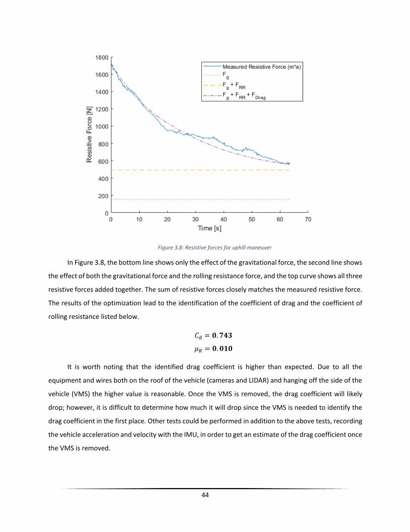
44
Figure 3.8: Resistive forces for uphill maneuver
In Figure 3.8, the bottom line shows only the effect of the gravitational force, the second line shows
the effect of both the gravitational force and the rolling resistance force, and the top curve shows all three
resistive forces added together. The sum of resistive forces closely matches the measured resistive force.
The results of the optimization lead to the identification of the coefficient of drag and the coefficient of
rolling resistance listed below.
𝐶𝑑 = 𝟎. 𝟕𝟒𝟑
𝜇𝑅 = 𝟎. 𝟎𝟏𝟎
It is worth noting that the identified drag coefficient is higher than expected. Due to all the
equipment and wires both on the roof of the vehicle (cameras and LIDAR) and hanging off the side of the
vehicle (VMS) the higher value is reasonable. Once the VMS is removed, the drag coefficient will likely
drop; however, it is difficult to determine how much it will drop since the VMS is needed to identify the
drag coefficient in the first place. Other tests could be performed in addition to the above tests, recording
the vehicle acceleration and velocity with the IMU, in order to get an estimate of the drag coefficient once
the VMS is removed.

45
The test was repeated multiple times both up and down the runway. Figure 3.9 shows the results
from the downhill test as opposed to the uphill test. The gravitational force for this curve is negative since
the gravitational force was pushing the vehicle forward as opposed to resisting the movement. It is also
worth noting that on the downhill test the vehicle didn’t slow down as much since there was less resistive
force acting on the vehicle. Consequentially the variation in the drag force forces are reduced since the
change in vehicle speed is reduced.
Figure 3.9: Resistive forces for downhill maneuver
In both Figure 3.8 and Figure 3.9 there are sections where the measured resistive force deviates
from the calculated resistive force. This can happen for many reasons, such as a change in the wind, a
slight change in road slope, or a bump on the road. The road slope was assumed to be constant throughout
the runway; however, in reality the road slope is not constant and as such the gravitational force should
not be a constant value. This is assumed to be the main contributor to the small errors.
Ultimately the full vehicle dynamic model will be used for simulation and control purposes. As such
it is more important that the velocities of the model match up with experimental results as opposed to
comparing the resistive forces. Figure 3.10 shows the measured and simulated velocity of the vehicle over

46
time. The data was normalized in order to compare the data from multiple runs. The velocity of the vehicle
was divided by the initial velocity and the time was divided through by the total time of the maneuver.
Figure 3.10: Dimensionless velocity versus time comparison between experimental results and simulated model
Even though there are minor deviations in the measured and simulated forces, the measured and
simulated velocities match quite closely. As mentioned earlier, the identified coefficient of drag includes
all the drag effects of the VMS. Once the VMS is removed the coefficient of drag will need to be modified.
Similarly, if additional hardware is added to the roof of the vehicle that will further change the drag
characteristics of the vehicle.

47
3.2.4. Suspension
3.2.4.1. 4-Post Testing
4-Post testing was conducted on the vehicle by Multimatic [54] as detailed in Section 2.2.4. They
were able to identify the spring constant and damping coefficient of the car; however, since the vehicle
has a semi-active suspension system, the values identified will not always be accurate. Due to the
limitations of 4-post testing, the vehicle must remain in park during testing. While the vehicle is in park,
the semi-active suspension system is not active. Consequentially the 4-post testing cannot help to identify
the semi-active control logic.
It was also mentioned by Multimatic that the observed spring behaviour was highly non-linear.
Unfortunately. the standard model they use for identification can only handle a linear spring, so the spring
constant for an idealized linear spring was provided. Figure 3.11 shows the model used by Multimatic in
order to identify the suspension parameters.
Figure 3.11: Suspension model for 4-post testing
The raw test data was provided in addition to the identified suspension values. A colleague,
Marshall Mykietyshyn, processed all the provided data and identified similar values, validating the values
received. Table 3.4 shows the values identified by Multimatic and Marshall Mykietyshyn [42]. The
estimated values are close to the identified values. Since the parameters from Multimatic have been
validated, they are used as the starting values during the next set of suspension testing outlined in Section
3.2.4.2.

48
Multimatic Values Estimated Values
Parameter Units Front Rear Front Rear
Installation Stiffness [N/mm] 520.8 754.0 518 740
Tire Stiffness [N/mm] 388.8 344.9 380 355
Suspension Stiffness [N/mm] 54.59 56.25 43 40
Suspension Damping [Ns/mm] 56.16 38.06 61 31
Table 3.4: Suspension parameter identification using data from 4-post testing
3.2.4.2. Road Testing
Starting with the values determined in Table 3.4, further work is needed to determine how the
damping coefficient changes based on the vehicle’s movement. First, a brief analysis of the suspension
stiffness is done to validate the results. Based on the model in Figure 3.11, a simple free body diagram of
the tire is developed.
Figure 3.12: Free body diagram of one tire
The free body diagram above is used to formulate the force balance equation in Equation 3.22.
𝐹𝑆𝑝𝑟𝑖𝑛𝑔 + 𝐹𝐷𝑎𝑚𝑝𝑒𝑟 − 𝐹𝑇𝑖𝑟𝑒 = 𝑚𝑊ℎ𝑒𝑒𝑙𝑎𝑊ℎ𝑒𝑒𝑙
(3.22)
The mass of the wheel is known. The acceleration of the wheel is determined by using the LGS
readings for wheel height and numerically differentiating twice. This introduces some error, but it was
found to be negligible. The tire force is measured through the WFS, leaving only the forces from the spring
and damper forces. Using the identified spring constant from the 4-post testing, the damping force can
be isolated. Figure 3.13 shows the damping force with respect to the rate of change in spring compression.

49
Figure 3.13: Damping force versus rate of change of suspension compression
Based on Figure 3.13 the damping force seems to be highly dependent on position rather than
velocity. As the spring compresses (negative velocity) the damping force goes from positive to negative.
At some compression point there is zero damping force even though there is still some velocity. This may
be because of the damping control law; however, it may also be because of the spring constant identified
from the 4-post testing. The later possibility is confirmed by observing the damping force while the
velocity is zero. The damper is still only able to produce force when the suspension is
compressing/decompressing, just like a normal damper. This means that the damping force is zero when
the suspension is not moving, contrary to what is seen in Figure 3.13. Consequentially the spring forces
must be re-evaluated.
The moments when the suspension is not moving are found by numerically differentiating the
values received from the WPS. All times when the value is near zero are moments when the suspension
is not moving. By using data only from these moments, where the damping force is known to be zero, the
spring force can be found. Assuming a linear spring, shown in Equation 3.23, the spring constant, k, is
solved for as seen in Equation 3.24.
𝐹𝑆𝑝𝑟𝑖𝑛𝑔 = 𝑘(𝑥 − 𝑙0)
(3.23)
𝑘(𝑥 − 𝑙0) = 𝑚𝑊ℎ𝑒𝑒𝑙𝑎𝑊ℎ𝑒𝑒𝑙 + 𝐹𝑇𝑖𝑟𝑒 (3.24)

50
𝑘 =𝑚𝑊ℎ𝑒𝑒𝑙𝑎𝑊ℎ𝑒𝑒𝑙 + 𝐹𝑇𝑖𝑟𝑒
(𝑥 − 𝑙0)
Figure 3.14 shows the spring constant versus spring compression from Equation 3.24. The results
show that the spring is highly non-linear, corroborating what Multimatic had observed. In fact the spring
can be represented by the exponential function shown in Equation 3.25.
𝑘 = 𝟔𝟎𝟒, 𝟓𝟎𝟎𝒆(−𝟐𝟓.𝟕𝒙) [𝑵𝒎] (3.25)
Figure 3.14: Non-linear behaviour of suspension spring
Based on Equation 3.24, the spring force is found for every data point and used to solve for the
damping force in Equation 3.22. Figure 3.15 shows the resulting damping force with respect to the rate of
change in spring compression.
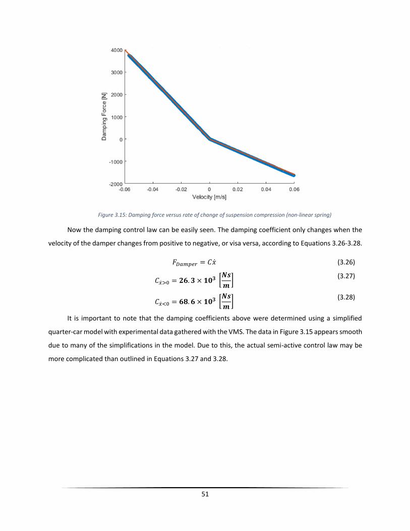
51
Figure 3.15: Damping force versus rate of change of suspension compression (non-linear spring)
Now the damping control law can be easily seen. The damping coefficient only changes when the
velocity of the damper changes from positive to negative, or visa versa, according to Equations 3.26-3.28.
𝐹𝐷𝑎𝑚𝑝𝑒𝑟 = 𝐶�̇� (3.26)
𝐶�̇�>0 = 𝟐𝟔. 𝟑 × 𝟏𝟎𝟑 [
𝑵𝒔
𝒎]
(3.27)
𝐶�̇�<0 = 𝟔𝟖. 𝟔 × 𝟏𝟎𝟑 [
𝑵𝒔
𝒎]
(3.28)
It is important to note that the damping coefficients above were determined using a simplified
quarter-car model with experimental data gathered with the VMS. The data in Figure 3.15 appears smooth
due to many of the simplifications in the model. Due to this, the actual semi-active control law may be
more complicated than outlined in Equations 3.27 and 3.28.

52
3.2.4.3. Single/Double Equivalent Kinematic Joints
One important feature of the suspension system is the trajectory of wheel travel. In many models
it is assumed that the suspension only allows vertical travel; however, as the suspension compresses and
decompresses, the camber and toe angles also change slightly. Normally, to identify the suspension
trajectory an in-depth analysis of the kinematic assembly of the suspension is required. With the WPS this
can be completed much easier through the use of single and double equivalent kinematic joints (SEK/DEK
joints) [55]. These joints express all wheel motion – lateral, longitudinal, camber angle and toe angle – as
functions of the vertical movement of the tire.
The vehicle chassis was raised by a single corner in order to measure the change in wheel position.
Ideally, the entire chassis would be lifted and suspended above the ground using a full vehicle lift. Then
each wheel could be lifted and measured independently. Unfortunately this was not possible with the
equipment available. Instead the chassis was raised near each of the wheels in turn. Resultantly, the
change in longitudinal and lateral positions is erroneous due to the tires contact with the ground. In
general, these values do not vary greatly and can be ignored without introducing significant of error.
Figure 3.16 shows the change in height of the wheel over time.
Figure 3.16: Change in wheel height over time
During the beginning of the test the car was raised through the use of a jack. This is the cause of
the step-like features. Once the limit of motion was reached, where the wheel and chassis were moving

53
in tandem, the jack slowly lowered the vehicle back to the ground. Figure 3.17 shows the lateral position
vs. height. The point (0,0) in the figure is arbitrary and depends on the installation conditions.
Consequentially, only the relative displacements are important. The smallest Z-Position value (-554)
represents the spring at full extension. Likewise, a smaller Y-Position value represents the tire being
further from the center of the vehicle. Therefore, as the spring extends, the wheel moves inwards, closer
to the center of the vehicle as is expected.
Figure 3.17: Lateral position of the wheel with respect to the vertical position of the wheel
The curve should look like a single line, but two distinct curves can be seen. One represents the
raising of the chassis and the second represents the lowering of the chassis. The ends of these curves
should be in the same location since the tire should not have moved, but due to the tire contact with the
ground, external forces have caused the ending locations to be slightly different. Due to this error, the
longitudinal and lateral results have been ignored. For future testing, the vehicle should be lifted off the
ground first to avoid erroneous data.
The camber and toe angles are plotted with respect to the height of the wheel in Figure 3.18 and
Figure 3.19 respectively.

54
Figure 3.18: Camber angle of the wheel with respect to the vertical position of the wheel
Figure 3.19: Toe angle of the wheel with respect to the vertical position of the wheel
It is worth noting that the change in toe angle is small and was later deemed inconsequential. To
simplify the model the change in toe angle is ignored, leaving camber angle as the only remaining variable.
The camber angle data is put through a spline-generating program in order to generate equations that
relate the camber angle of the tire with the change of height between the tire and the chassis. A custom
Matlab code is used in order to convert these splines into kinematic constraint equations which are then
implemented in a custom MapleSim joint used for the suspension.

55
3.2.5. Tire Modelling
To use the data for tire modeling, some processing must be done. Primarily, the sideslip angle and
longitudinal slip ratio must be calculated. Longitudinal slip is defined in Equation 1.1. Since longitudinal
slip is calculated by dividing through by the vehicle speed, all test points where the vehicle speed is zero
will cause a singularity. These data points generally all occur before or after the test maneuvers and must
be removed.
The sideslip angle is calculated by observing the longitudinal and lateral speed of the tire, measured
by the LGS. If there is no lateral speed, then the tire heading is the same as the tire direction of motion,
meaning the sideslip angle is zero. If lateral speeds are observed then the resultant direction of motion is
found using the Pythagorean theorem. A simple trigonometric identity gives the sideslip angle of the tire.
This is outlined in Equation 3.29. Note that the longitudinal and lateral speeds are in the local tire frame.
𝛼 = tan−1 (
𝐿𝑎𝑡𝑒𝑟𝑎𝑙 𝑆𝑝𝑒𝑒𝑑
𝐿𝑜𝑛𝑔𝑖𝑡𝑢𝑑𝑖𝑛𝑎𝑙 𝑆𝑝𝑒𝑒𝑑)
(3.29)
As described in Section 1.3.2, the tire forces depend upon the normal load experienced by the tire.
The normal load on the tire is measured and can be accounted for in the model. This is done by dividing
the recorded longitudinal and lateral forces by the normal load. This normalization accounts for all the
changes in tire behavior due to normal load. The normalized longitudinal Pacejka tire model is shown in
Equation 3.30.
𝐹𝑥
𝐹𝑧
(𝑠) = 𝐷 sin(𝐶 tan−1(𝐵𝑠 − 𝐸(𝐵𝑠 − tan−1(𝐵𝑠))))
(3.30)
It is assumed that the parameters of the Pacejka tire model do not vary based on normal load. In
other words, it is assumed that the longitudinal force is directly proportional to the normal load on the
tire, and can be normalized according to Equation 3.30. This assumption is consistent with the 1989
version of the Pacejka tire model.
Some post-processing must also be done using measurements from the WPS. During more extreme
testing maneuvers, the camber angle of the tires increase. The reference frame of the WFS is fixed to the
wheel. Based on this, as the toe and camber angles increase, part of the normal load is actually measured
as a lateral force, and vice versa. The toe and camber angles are measured using the WPS. Based on
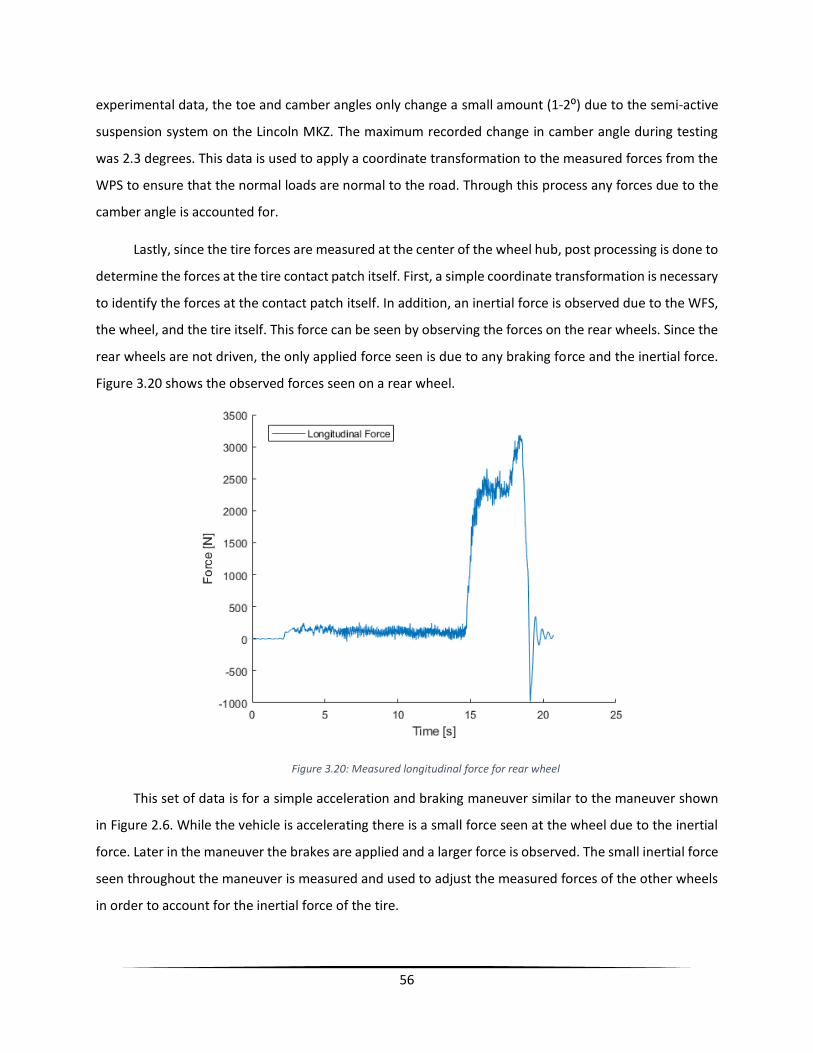
56
experimental data, the toe and camber angles only change a small amount (1-2⁰) due to the semi-active
suspension system on the Lincoln MKZ. The maximum recorded change in camber angle during testing
was 2.3 degrees. This data is used to apply a coordinate transformation to the measured forces from the
WPS to ensure that the normal loads are normal to the road. Through this process any forces due to the
camber angle is accounted for.
Lastly, since the tire forces are measured at the center of the wheel hub, post processing is done to
determine the forces at the tire contact patch itself. First, a simple coordinate transformation is necessary
to identify the forces at the contact patch itself. In addition, an inertial force is observed due to the WFS,
the wheel, and the tire itself. This force can be seen by observing the forces on the rear wheels. Since the
rear wheels are not driven, the only applied force seen is due to any braking force and the inertial force.
Figure 3.20 shows the observed forces seen on a rear wheel.
Figure 3.20: Measured longitudinal force for rear wheel
This set of data is for a simple acceleration and braking maneuver similar to the maneuver shown
in Figure 2.6. While the vehicle is accelerating there is a small force seen at the wheel due to the inertial
force. Later in the maneuver the brakes are applied and a larger force is observed. The small inertial force
seen throughout the maneuver is measured and used to adjust the measured forces of the other wheels
in order to account for the inertial force of the tire.

57
3.2.5.1. Pure Longitudinal Slip Pacejka Model
The normalized pure longitudinal slip Pacejka model, detailed in Equation 3.30, depends solely on
longitudinal slip. As stated earlier, many other factors also influence the longitudinal force. Many of these
factors are taken into account during data processing, such as inertial force; however, many of these
factors are also ignored in order to simplify the model, such as wheel temperature and variable road
friction. Note that all tire testing was completed on dry pavement during warm summer months. Figure
3.21 shows the processed data for the pure longitudinal slip acceleration/braking test. The x-axis is the
longitudinal slip and the y-axis is the dimensionless normalized longitudinal force. It is assumed that the
tire pressure remains constant throughout the test. Each tire was inflated to 35 psi before each round of
testing to ensure the pressure remained at a known constant value.
Figure 3.21: Measured data from pure longitudinal slip test
It can be seen that many of these data points are erroneous. There should be no high slip values
that provide a near-zero force. These data points are all erroneous values that occur when the vehicle is
at a near-zero speed. From the definition of longitudinal slip, it can be seen that when the vehicle speed
is near-zero the slip values are more prone to error. Post-processing removes all singularities by removing
all data points with a vehicle speed of zero; however, near-zero speeds will also cause erroneous data due
to the asymptote. By removing these values, a more representative data set is obtained.

58
Using this data set, a nonlinear least squares optimizing routine is performed to identify the Pacejka
parameters in Equation 3.30. This was done using the Matlab Curve Fitting toolbox. The parameters for
this Pacejka tire model are provided in the Appendix. The resulting Pacejka curve is shown with the
experimental data set in Figure 3.22. In addition, a linear tire model is also fit to show a comparison
between these two models.
Figure 3.22: Normalized longitudinal force versus pure longitudinal slip
The linear tire model shown in Figure 3.22 is accurate for small values of longitudinal slip. The linear
tire model is much simpler than the Pacejka model; however, the use of the linear tire model is limited.
Likewise, the pure longitudinal slip 1989 Pacejka tire model is much simpler than other tire models like
the 2012 Pacejka or TAME models, so it also has limited use as detailed in Section 1.3.2.
The pure longitudinal slip Pacejka model was developed using data points from every run of the
test specified in the Section 2.2.5. It is worth noting that when performing the optimization for only the
data points for each individual run, the resulting parameters only differ by a maximum of 1.8%. This helps
validate the repeatability of the designed test.

59
3.2.5.2. Pure Lateral Slip Pacejka Model
The pure lateral slip model is determined in a similar fashion as the pure longitudinal slip; however,
instead of longitudinal slip, the sideslip angle is used. Sideslip is defined as the angle between the heading
of the wheel and the instantaneous direction of motion of the wheel. Details for calculating the sideslip
angle based on experimental data are found near the beginning of Section 3.2.5. Like the longitudinal
model, the lateral tire force is divided through by the normal load to calculate the normalized lateral force.
By normalizing the lateral force, the change in lateral force due to the normal load is accounted for.
Like the pure longitudinal slip model, there are a number of erroneous data points while the vehicle
is near zero speed. This is due to the calculation of the sideslip angle, calculated by dividing by the
longitudinal speed of the wheel. After removing the erroneous data while the vehicle was near zero speed
and combining the data from each of the three different tests performed, a comprehensive data set is
achieved. The data points are plotted in Figure 3.23. An optimization routine is run in order to determine
the Pacejka curve parameters necessary for the model to fit the data. The parameters for this curve are
shown in the Appendix.
Figure 3.23: Normalized lateral force versus pure sideslip
60
It is worth noting that the experimental data points shown in Figure 3.23 have a higher standard
deviation than the longitudinal results in Figure 3.22. This is seen as the thickness of the experimental
curve. The standard deviation is larger due to multiple reasons. Primarily it is due to many of the
simplifications that were used for this model, such as neglecting camber thrust and temperature changes.
It was observed that the tire temperature varied more during the lateral tests than during the longitudinal
test.
The increased standard deviation is also likely due to the normalization process. The normal load
observed on the tires vary more during the lateral tests as opposed to the longitudinal tests. These
transients increase the standard deviation.
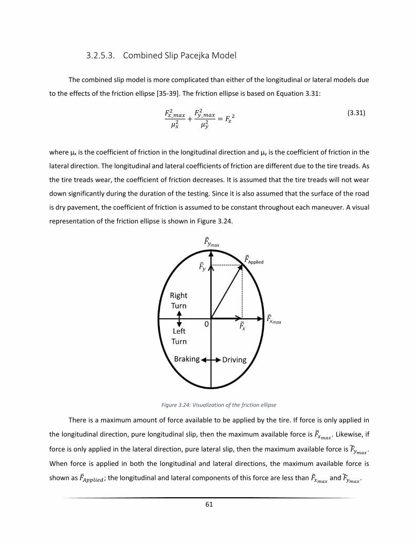
61
3.2.5.3. Combined Slip Pacejka Model
The combined slip model is more complicated than either of the longitudinal or lateral models due
to the effects of the friction ellipse [35-39]. The friction ellipse is based on Equation 3.31:
𝐹𝑥_𝑚𝑎𝑥2
𝜇𝑥2 +
𝐹𝑦_𝑚𝑎𝑥2
𝜇𝑦2 = 𝐹𝑧
2
(3.31)
where μx is the coefficient of friction in the longitudinal direction and μy is the coefficient of friction in the
lateral direction. The longitudinal and lateral coefficients of friction are different due to the tire treads. As
the tire treads wear, the coefficient of friction decreases. It is assumed that the tire treads will not wear
down significantly during the duration of the testing. Since it is also assumed that the surface of the road
is dry pavement, the coefficient of friction is assumed to be constant throughout each maneuver. A visual
representation of the friction ellipse is shown in Figure 3.24.
Figure 3.24: Visualization of the friction ellipse
There is a maximum amount of force available to be applied by the tire. If force is only applied in
the longitudinal direction, pure longitudinal slip, then the maximum available force is �̃�𝑥𝑚𝑎𝑥. Likewise, if
force is only applied in the lateral direction, pure lateral slip, then the maximum available force is �̃�𝑦𝑚𝑎𝑥.
When force is applied in both the longitudinal and lateral directions, the maximum available force is
shown as �̃�𝐴𝑝𝑝𝑙𝑖𝑒𝑑; the longitudinal and lateral components of this force are less than �̃�𝑥𝑚𝑎𝑥 and �̃�𝑦𝑚𝑎𝑥
.

62
Under normal driving situations this effect is not prevalent due to the low magnitude of the lateral
force. The purpose of developing these models is to implement them on an autonomous vehicle. Most
maneuvers the vehicle will perform are normal driving situations where this effect is not substantial;
however, in a safety-critical situation where an autonomous vehicle must try to avoid an obstacle, this
reduced maximum force is vital information.
Because of this, a combined slip model is developed. The following work is completed for both the
longitudinal and lateral combined slip models; however, since the process for both of these models is
identical, only the longitudinal work will be presented. The data gathered through the two combined slip
tests are compiled together and any erroneous data is removed, just as it was in the pure slip models. To
determine if there is actually a large effect on available forces during combined slip conditions, the
normalized longitudinal force is plotted against the normalized lateral force. The resulting plot is cluttered
due to the large number of data points. Many of the data points were trimmed for visualization, shown in
Figure 3.25.
Figure 3.25: Normalized longitudinal force versus normalized lateral force
It is worth noting that every point inside the friction ellipse is a feasible point. The tires do not need
to apply the maximum available force, rather they are limited by the maximum force. This is why many of

63
the data points in Figure 3.25 are arrayed inside the border of the ellipse. As the sideslip values increase,
the longitudinal force observed decreases while the lateral force increases. Only a few of the data points
for larger sideslip values are shown; however, it is easy to see that as the lateral force increases the
available longitudinal force decreases. It is important to note that the high lateral force values only occur
during high sideslip values as expected. The low lateral forces shown for near zero sideslip values are
necessary for vehicle stability.
From Figure 3.25 it is seen that as the absolute value of the lateral force increases, the longitudinal
force decreases. Consequentially, the longitudinal slip was plotted against the normalized longitudinal
force to determine the differences in the longitudinal Pacejka model. This can be seen in Figure 3.26. By
adding a third dimension for the sideslip (different colors), one can see the impact it has on the available
longitudinal force.
Figure 3.26: Longitudinal slip versus normalized longitudinal force with varying sideslip
The most substantial change is seen when observing the data points with a sideslip angle of twenty
degrees. It is clear that if a linear tire model was optimized around these data points, as opposed to the
near zero sideslip data points, the slope of the model would be significantly different. This is the main
impact that needs to be captured by the combined slip tire model.

64
It is important to note that large sideslip values are only shown in the negative longitudinal slip
(braking) range. The sideslip values observed in the positive longitudinal slip range are ignored only for
visualization purposes; they are included in calculations. In addition, it is worth noting that sideslip values
exceeding 15 degrees are only seen in the braking region. This is expected, due to mechanical limitations,
as outlined in Section 2.2.5. The combined slip models will mainly be used in safety critical situations,
when the only objective is avoiding an obstacle. During these types of situations, it is likely that the vehicle
will attempt to steer away from the obstacle while braking, not accelerating. Consequentially, the
combined slip models are optimized more for the braking region than the accelerating region.
To create a combined slip model, a continuous function is needed to account for the change in
longitudinal forces due to lateral forces and vice versa. This is accomplished by creating a piecewise
function and then fitting a spline to link the identified data points.
Using specific data points, multiple Pacejka curves are optimized around the different sideslip
values. Curves are optimized for sideslip values of 0 (pure longitudinal slip), 2, 5, 10, 15, 20, and 25
degrees. These values were chosen due to the distribution of data points. The optimization process is
identical to the process outlined in the pure slip models. More values can be used to increase the fidelity
of the model. Assuming symmetry consistent with the Pacejka model, identical curves are used for each
corresponding negative sideslip value. To increase the fidelity, new curves could be fitted for this negative
region. The identified Pacejka parameters are presented in the Appendix along with the parameters for
the lateral combined slip Pacejka curves.
Three of the resulting curves, for 0, 10, and 20 degrees sideslip angle, are shown in Figure 3.27. The
experimental data shown in Figure 3.27 is the same as that in Figure 3.26; however the sideslip values
were ignored for visualization to highlight the three different curves.

65
Figure 3.27: Combined slip Pacejka models for sideslip values of 0, 10, and 20 degrees
As sideslip angle increases, the maximum available longitudinal force decreases significantly. This
decrease is not linear, which is why the piecewise functions are necessary to obtain an accurate
representation of the full combined slip model. This data could be used to determine the parameters of
the 2012 Pacejka model. This would eliminate the piecewise nature of the current model; however, it
would also require increasing the complexity of the model significantly. There are other methods that will
eliminate the piecewise nature of the combined slip Pacejka model without having to identify the large
number of parameters needed in the 2012 Pacejka model.
One such method was developed by MSC Software for use in the 1989 and 1994 Pacejka models
[47]. This method involves modifying the coefficient of friction values in order to change the available
forces due to combined slip behavior. This is best seen by referring back to the equation for the friction
ellipse, Equation 3.31. The coefficients of friction in both the longitudinal and lateral directions become
functions of longitudinal slip and lateral sideslip. As the coefficients of friction change, the available forces
in each of those directions will also change. Referring to Figure 3.25, the indicated force could be achieved
by reducing the coefficient of friction in both directions so as to reduce the maximum forces to the
indicated available forces. This method works well when only the pure slip Pacejka models are known, but
since the combined slip models have also been developed here, it is not necessary.
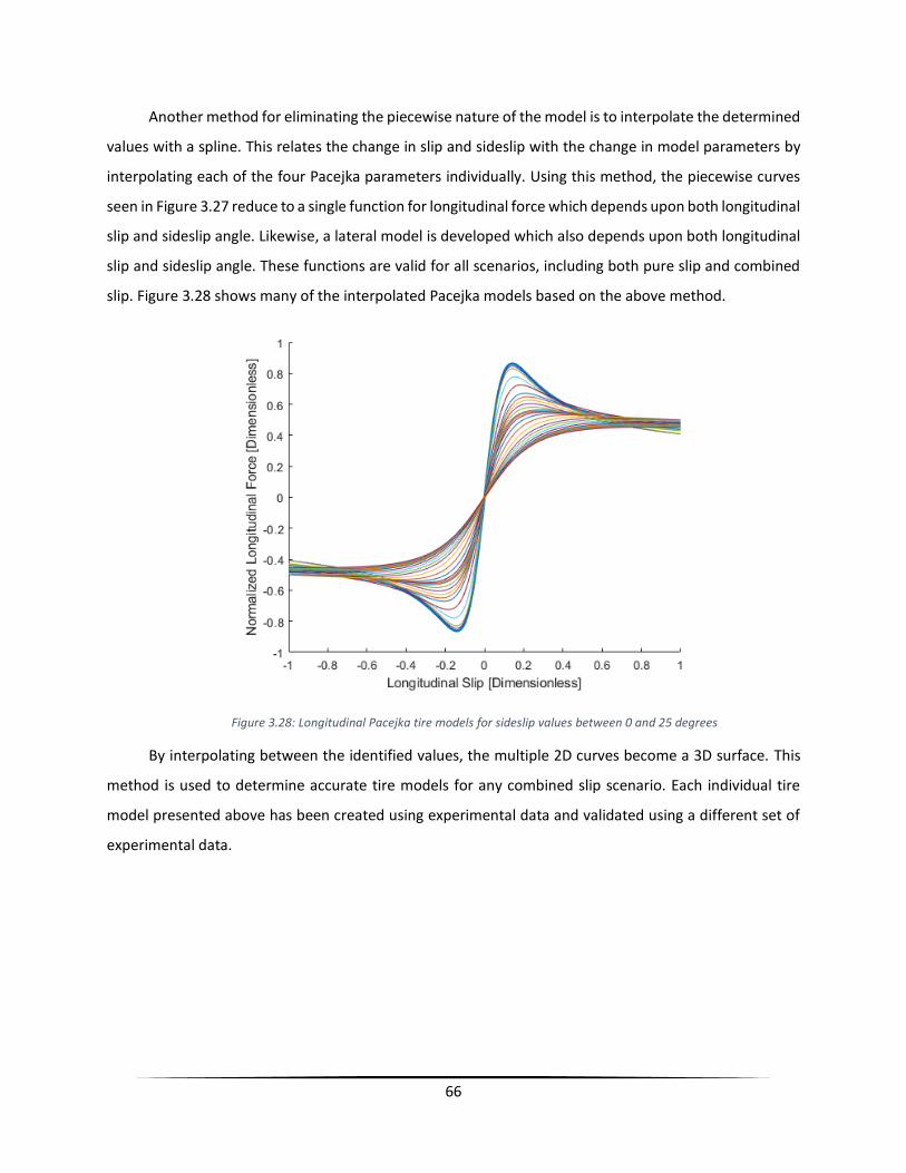
66
Another method for eliminating the piecewise nature of the model is to interpolate the determined
values with a spline. This relates the change in slip and sideslip with the change in model parameters by
interpolating each of the four Pacejka parameters individually. Using this method, the piecewise curves
seen in Figure 3.27 reduce to a single function for longitudinal force which depends upon both longitudinal
slip and sideslip angle. Likewise, a lateral model is developed which also depends upon both longitudinal
slip and sideslip angle. These functions are valid for all scenarios, including both pure slip and combined
slip. Figure 3.28 shows many of the interpolated Pacejka models based on the above method.
Figure 3.28: Longitudinal Pacejka tire models for sideslip values between 0 and 25 degrees
By interpolating between the identified values, the multiple 2D curves become a 3D surface. This
method is used to determine accurate tire models for any combined slip scenario. Each individual tire
model presented above has been created using experimental data and validated using a different set of
experimental data.

67
3.3. Parameter Identification Using High Fidelity
Vehicle Dynamic Model
After all parameter identification was completed as described in Section 3.2, the parameters were
entered into the MapleSim model and a full parameter optimization routine was run. The vehicle model
was exported as a Simulink function where a non-linear least squares optimization routine was run to find
the parameters that minimized the relative error between the full vehicle model outputs and the
experimental results. A series of tests were performed similar to the tests outlined in Section 2.2. Several
additional tests were performed at random to ensure that the model was accurate. All parameter values
were not allowed to change by more than 25% of the values found from the simpler models found in
Section 3.2. This was done to ensure that the optimized values were still feasible. The final parameter
values can be found in Appendix B.
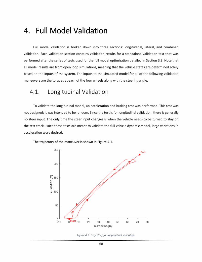
68
4. Full Model Validation
Full model validation is broken down into three sections: longitudinal, lateral, and combined
validation. Each validation section contains validation results for a standalone validation test that was
performed after the series of tests used for the full model optimization detailed in Section 3.3. Note that
all model results are from open loop simulations, meaning that the vehicle states are determined solely
based on the inputs of the system. The inputs to the simulated model for all of the following validation
maneuvers are the torques at each of the four wheels along with the steering angle.
4.1. Longitudinal Validation
To validate the longitudinal model, an acceleration and braking test was performed. This test was
not designed; it was intended to be random. Since the test is for longitudinal validation, there is generally
no steer input. The only time the steer input changes is when the vehicle needs to be turned to stay on
the test track. Since these tests are meant to validate the full vehicle dynamic model, large variations in
acceleration were desired.
The trajectory of the maneuver is shown in Figure 4.1.
Figure 4.1: Trajectory for longitudinal validation

69
The maneuver includes three relatively straight-line paths down the length of the test track. The
trajectory is generated using the GPS values from the VBox. The longitudinal velocity of the vehicle is
found by integrating the acceleration measured with the IMU. The experimental and simulated velocities
are shown in Figure 4.2.
Figure 4.2: Longitudinal velocity versus time for longitudinal validation
It is worth noting that the two sections where the experimental data and simulation results vary
significantly are found during 20-30s and 55-65s. These are the two times in the maneuver where the
vehicle is turned around. During these sections, the vehicle speed is very small and the experimental data
from the IMU is less accurate due to the small changes in vehicle acceleration. This can be seen as an
excess level of noise in the experimental values.
Most of the smaller deviations occur after large braking regions. This is common throughout all
validation results and is due to the lack of experimental data at the rear right wheel. Since the vehicle is a
front wheel drive, the rear wheels only apply torques during braking maneuvers. Due to a sensor
malfunction, the rear right wheel of the vehicle was not measured during testing and could not be used
as an input to the simulation model. Instead, it was assumed that the same braking torques were applied
to both the rear left and rear right wheels. While this is the best approximation that can be determined
given the circumstances, it is not entirely accurate and may lead to erroneous data.
70
To accurately reproduce the vehicle motion in a simulation environment, the accelerations and
angular velocities of the vehicle model must match the experimental data. These values are used to
validate the model since they are captured directly using the IMU. The experimental data is compared
against the simulation data in Figure 4.3 and Figure 4.4.

71
Figure 4.3: Accelerations versus time for longitudinal validation
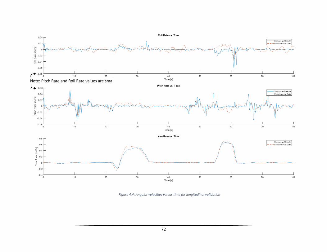
72
Figure 4.4: Angular velocities versus time for longitudinal validation
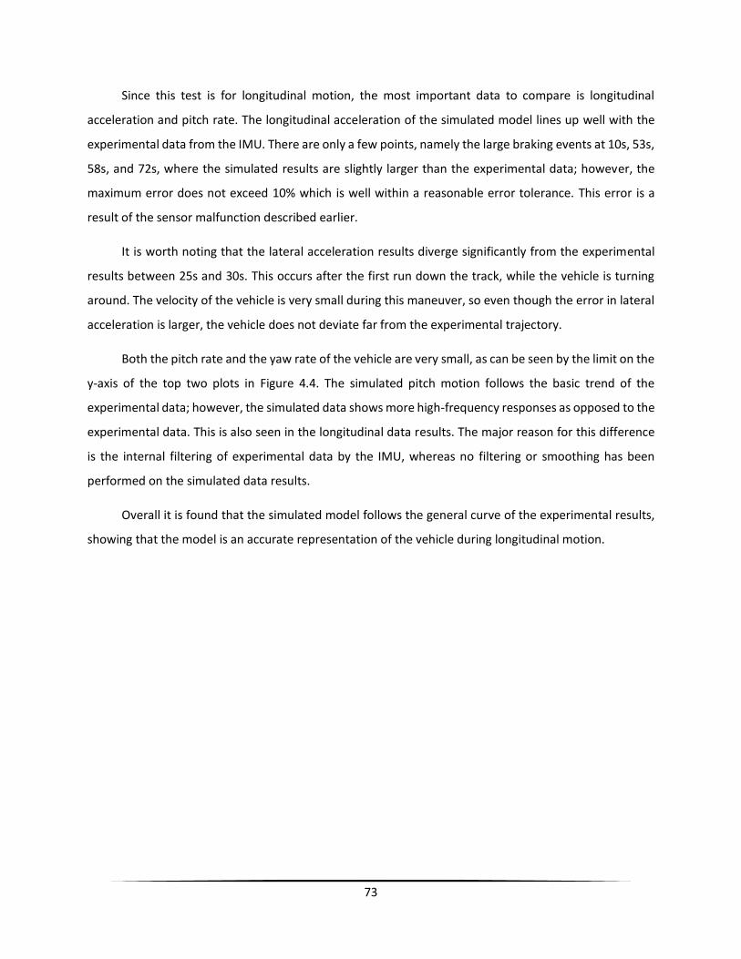
73
Since this test is for longitudinal motion, the most important data to compare is longitudinal
acceleration and pitch rate. The longitudinal acceleration of the simulated model lines up well with the
experimental data from the IMU. There are only a few points, namely the large braking events at 10s, 53s,
58s, and 72s, where the simulated results are slightly larger than the experimental data; however, the
maximum error does not exceed 10% which is well within a reasonable error tolerance. This error is a
result of the sensor malfunction described earlier.
It is worth noting that the lateral acceleration results diverge significantly from the experimental
results between 25s and 30s. This occurs after the first run down the track, while the vehicle is turning
around. The velocity of the vehicle is very small during this maneuver, so even though the error in lateral
acceleration is larger, the vehicle does not deviate far from the experimental trajectory.
Both the pitch rate and the yaw rate of the vehicle are very small, as can be seen by the limit on the
y-axis of the top two plots in Figure 4.4. The simulated pitch motion follows the basic trend of the
experimental data; however, the simulated data shows more high-frequency responses as opposed to the
experimental data. This is also seen in the longitudinal data results. The major reason for this difference
is the internal filtering of experimental data by the IMU, whereas no filtering or smoothing has been
performed on the simulated data results.
Overall it is found that the simulated model follows the general curve of the experimental results,
showing that the model is an accurate representation of the vehicle during longitudinal motion.
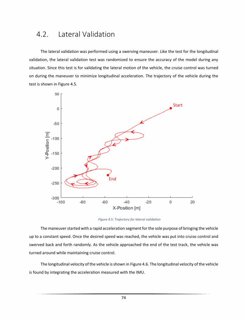
74
4.2. Lateral Validation
The lateral validation was performed using a swerving maneuver. Like the test for the longitudinal
validation, the lateral validation test was randomized to ensure the accuracy of the model during any
situation. Since this test is for validating the lateral motion of the vehicle, the cruise control was turned
on during the maneuver to minimize longitudinal acceleration. The trajectory of the vehicle during the
test is shown in Figure 4.5.
Figure 4.5: Trajectory for lateral validation
The maneuver started with a rapid acceleration segment for the sole purpose of bringing the vehicle
up to a constant speed. Once the desired speed was reached, the vehicle was put into cruise control and
swerved back and forth randomly. As the vehicle approached the end of the test track, the vehicle was
turned around while maintaining cruise control.
The longitudinal velocity of the vehicle is shown in Figure 4.6. The longitudinal velocity of the vehicle
is found by integrating the acceleration measured with the IMU.
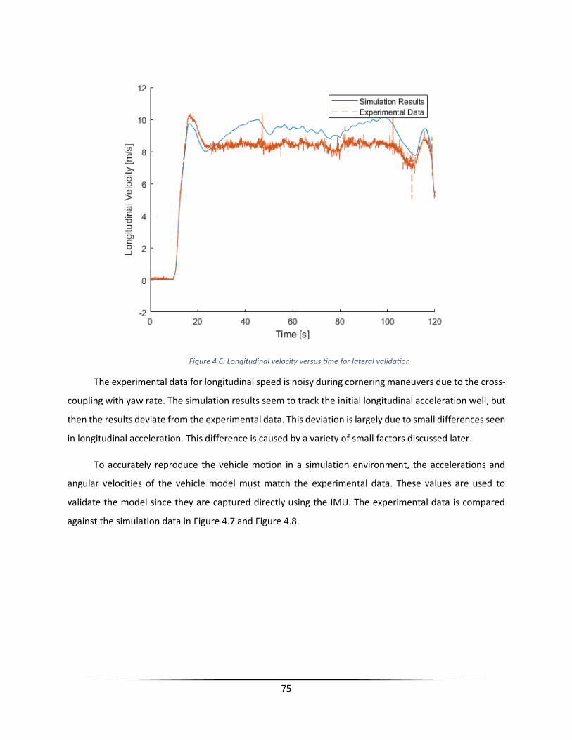
75
Figure 4.6: Longitudinal velocity versus time for lateral validation
The experimental data for longitudinal speed is noisy during cornering maneuvers due to the cross-
coupling with yaw rate. The simulation results seem to track the initial longitudinal acceleration well, but
then the results deviate from the experimental data. This deviation is largely due to small differences seen
in longitudinal acceleration. This difference is caused by a variety of small factors discussed later.
To accurately reproduce the vehicle motion in a simulation environment, the accelerations and
angular velocities of the vehicle model must match the experimental data. These values are used to
validate the model since they are captured directly using the IMU. The experimental data is compared
against the simulation data in Figure 4.7 and Figure 4.8.
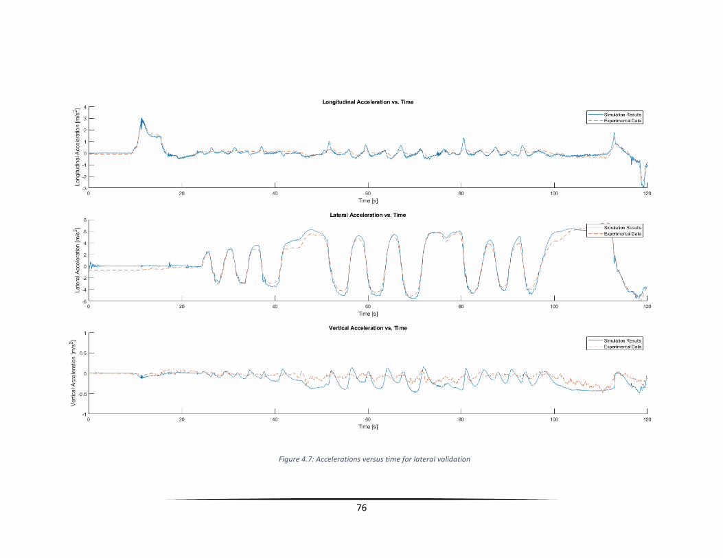
76
Figure 4.7: Accelerations versus time for lateral validation
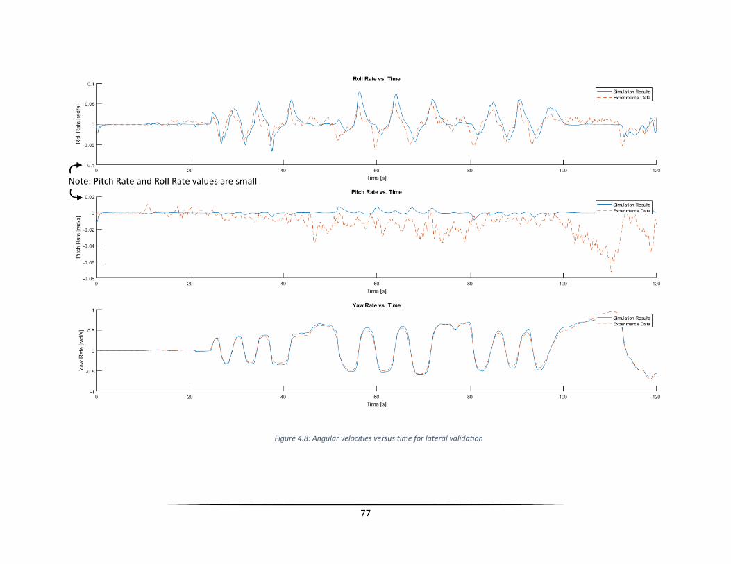
77
Figure 4.8: Angular velocities versus time for lateral validation
78
The longitudinal acceleration of the model closely matches that of the experimental data. Small
differences can be seen during the cruise control section of the maneuver. Mainly, the simulation results
in larger peak values than the experimental results. The primary reason for this error is the rear right
wheel torque input value to the simulated mode. Due to the sensor malfunction described in Section 4.1,
the rear right wheel of the vehicle was not measured during testing and could not be used as an input to
the simulation model, instead the same braking torques were applied to both rear wheels. By looking at
the experimental data it can be seen that this approximation is not very accurate during cornering
maneuvers.
The lateral acceleration of the model is close to the experimental results from testing. The general
trend of the curves are identical, and the peak values are nearly the same. The slight difference in peak
values may be due to the slight inaccuracy of the semi-active control law as explained in Section 3.2.4.2.
The results diverge slightly between 95s and 110s. This is likely due to cornering at a lower speed just like
the results seen in the longitudinal validation results. It is also worth noting that the IMU was not placed
at a known location on the vehicle. The approximate location is known but the exact coordinates are not
known. Consequentially the exact experimental measurements are not accurate. There is some error
introduced by estimating the location where the experimental data was collected.
For lateral validation, the roll rate and yaw rate vary the most. The pitch rate is very small as seen
by the y-axis limits. The roll rate of the model lines up very closely with the experimental results, even
considering the small magnitude of the values. The small errors seen here are likely due to the location of
the IMU, measurement noise, or the semi-active control law of the model.
The yaw rate of the simulated model matches almost exactly with the experimental results. The
only major deviation is seen between 95s and 110s for the same reasons as described earlier. Overall it is
found that the simulated model follows the general curve of the experimental results, showing that the
model is an accurate representation of the vehicle during lateral motion.

79
4.3. Combined Validation
The vehicle also needs to be validated under combined slip scenarios in order to test and validate
how the vehicle will react while undergoing both longitudinal and lateral motion simultaneously. Most
desired trajectories will involve the vehicle traveling under combined scenarios. For this test, the vehicle
was accelerated and decelerated rapidly while also performing a variety of cornering maneuvers. It was
ensured that the maneuver included acceleration, braking, and cornering events, along with various
combinations of these events, in order to test the full extent of the model accuracy. The trajectory of the
vehicle during this test is shown in Figure 4.9.
Figure 4.9: Trajectory for combined validation
The longitudinal velocity of the vehicle is shown in Figure 4.10. The longitudinal velocity of the
vehicle is found by integrating the acceleration measured with the IMU.

80
Figure 4.10: Longitudinal velocity versus time for combined validation
The velocity profile of the simulated model lines up closely with the experimental results. Most of
the deviations occur after large braking regions. The experimental acceleration and angular velocity data
is compared against the simulation data in Figure 4.11 and Figure 4.12.
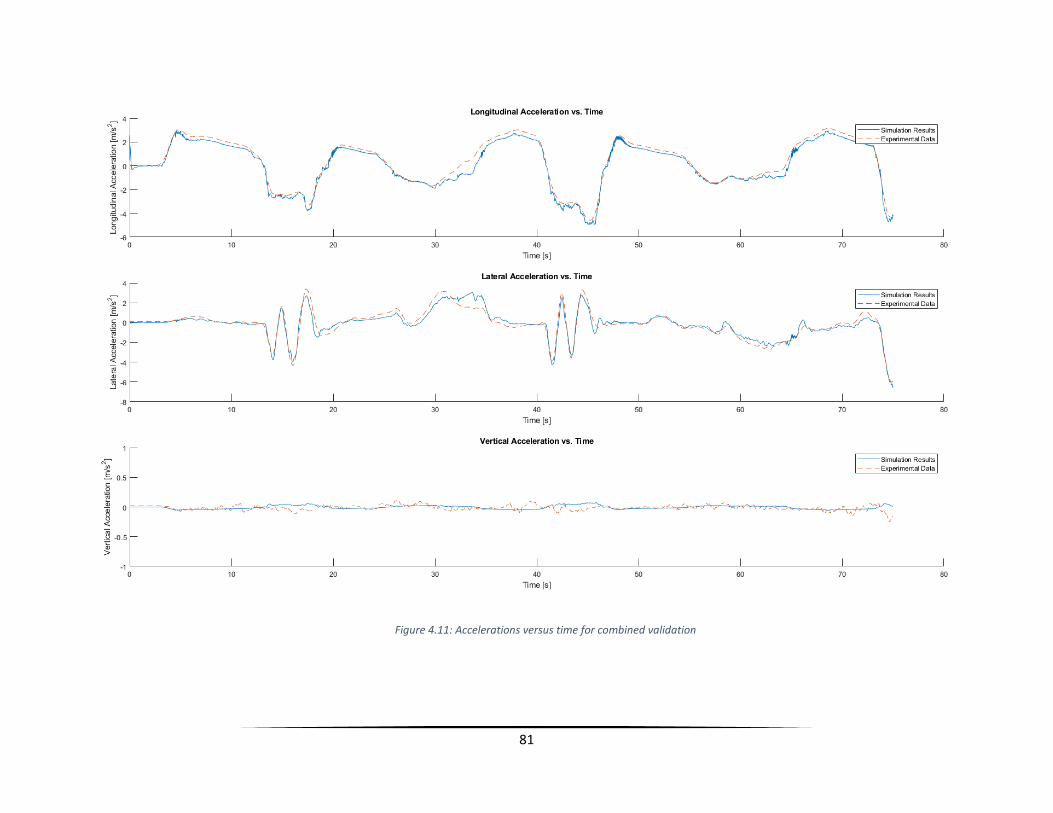
81
Figure 4.11: Accelerations versus time for combined validation

82
Figure 4.12: Angular velocities versus time for combined validation

83
The model results for the longitudinal, lateral, and vertical accelerations all match up very closely
with the experimental data. The only major deviation occurs between 30s and 35s. During this time the
vehicle was doing a 180⁰ turn in order to go back down the track. The only other time the vehicle fully
turns around is between 60s and 65s, where another minor deviation can be seen. Beyond these two
points, the simulation results line up very well with the experimental data, with the largest percent error
being under 5%.
The model results for the roll, pitch, and yaw rates also all line up closely with the experimental
data. The roll rate is fairly small, but the model results are practically identical to the experimental data
when larger roll rates are observed, such as those seen during the quick swerving maneuvers at 15s and
42s. The pitch rate is very small but the model results follow the general trend observed in the
experimental data. Lastly the yaw rate is observed. Like the lateral acceleration, the yaw rate lines up
closely with the experimental data, only deviating during the large turnaround moments during the
maneuver.
Overall, the combined validation shows that the full vehicle dynamic model is a reasonably accurate
representation of the physical vehicle.

84
5. Conclusions
5.1. Summary
In this thesis, a full car model was created with MapleSim 2017.3 using experimental data from on-
road testing alone. Specific road tests were designed to isolate desired parameter values in order to make
parameter identification easier. These tests were designed to be repeatable, both on the same test vehicle
and on other future test vehicles. Parameter identification was performed using a two-step process. First,
all the necessary model parameters including the center of mass location, the inertia values of the chassis
and wheels, the coefficient of drag, the suspension parameters, and the parameters for the combined slip
1989 Pacejka tire model were identified using simple models. Then a separate round of testing was
completed and used to further optimize all of the identified parameters simultaneously through the high
fidelity vehicle dynamic model. Lastly several different validation tests were performed in order to
observe the accuracy of the model. In longitudinal, lateral, and combined testing, the simulated model
results closely matched the experimental data. In conclusion, the identified model is a reasonably accurate
representation of the Moose which can support controller development and virtual reality simulation for
autonomous vehicle testing.
5.2. Future Work
There are many steps that can be taken to improve the full vehicle dynamic model. The primary
areas for improvement are the tire models and the suspension model. While the combined slip tire models
described in Section 3.2.5 are accurate, they are still based on a model from 1989; multiple improvements
to the Pacejka model have been made since then. These improvements account for many of the
transients, such as the rate of change of normal load, camber thrust, temperature changes, and road
friction. These additional details would increase the accuracy of the tire forces; however, extensive testing
would be needed to identify the 117 parameters needed for this model. The suspension model
incorporated in the vehicle dynamic model includes the non-linear spring and the piecewise linear
damper. In reality, the semi-active damping law is likely more complicated than a simple piecewise
function. Further testing is needed to determine the actual semi-active damping law, which can then
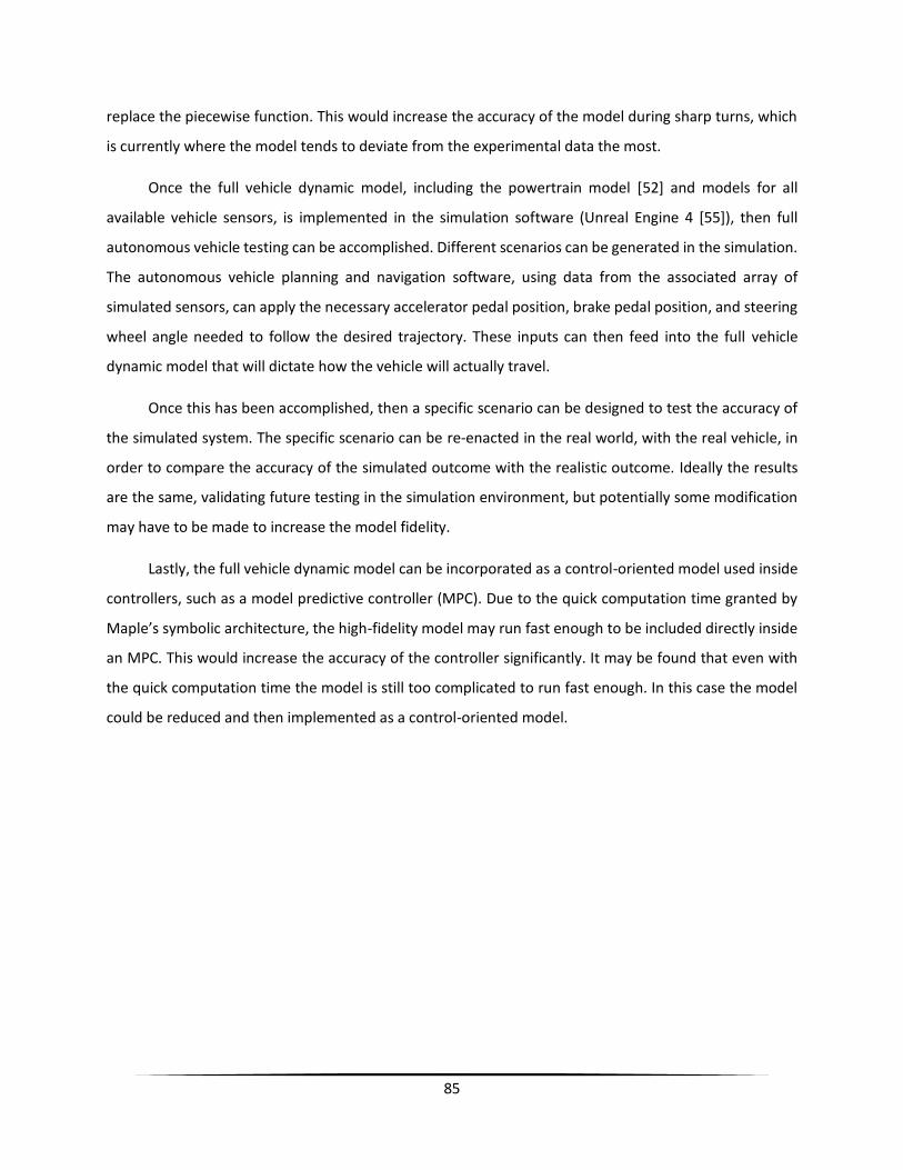
85
replace the piecewise function. This would increase the accuracy of the model during sharp turns, which
is currently where the model tends to deviate from the experimental data the most.
Once the full vehicle dynamic model, including the powertrain model [52] and models for all
available vehicle sensors, is implemented in the simulation software (Unreal Engine 4 [55]), then full
autonomous vehicle testing can be accomplished. Different scenarios can be generated in the simulation.
The autonomous vehicle planning and navigation software, using data from the associated array of
simulated sensors, can apply the necessary accelerator pedal position, brake pedal position, and steering
wheel angle needed to follow the desired trajectory. These inputs can then feed into the full vehicle
dynamic model that will dictate how the vehicle will actually travel.
Once this has been accomplished, then a specific scenario can be designed to test the accuracy of
the simulated system. The specific scenario can be re-enacted in the real world, with the real vehicle, in
order to compare the accuracy of the simulated outcome with the realistic outcome. Ideally the results
are the same, validating future testing in the simulation environment, but potentially some modification
may have to be made to increase the model fidelity.
Lastly, the full vehicle dynamic model can be incorporated as a control-oriented model used inside
controllers, such as a model predictive controller (MPC). Due to the quick computation time granted by
Maple’s symbolic architecture, the high-fidelity model may run fast enough to be included directly inside
an MPC. This would increase the accuracy of the controller significantly. It may be found that even with
the quick computation time the model is still too complicated to run fast enough. In this case the model
could be reduced and then implemented as a control-oriented model.

86
References
1. Li, K., Hang, Y., Jiang, Y., He, C., and Yue, W., "A Path Planning Method Based on Large Amount of
Artificial Driving Trajectories," SAE Technical Paper 2018-01-1588, 2018,
https://doi.org/10.4271/2018-01-1588.
2. Zhong, Y., Wang, S., Xie, S., Cao, Z., Jiang, K., and Yang, D., “3D Scene Reconstruction with Sparse
LiDAR Data and Monocular Image in Single Frame,” SAE Int. J. Passeng. Cars- Electron. Electr. Syst.
11(1):48-56, 2018, https://doi.org/10.4271/07-11-01-0005.
3. Hu, C., Wang, Y., Yu, G., Wang, Z., Lei, A., and Hu, Z., "Embedding CNN-Based Fast Obstacles
Detection for Autonomous Vehicles," SAE Technical Paper 2018-01-1622, 2018,
https://doi.org/10.4271/2018-01-1622.
4. Hu, Y. and Furukawa, T., "A High-Resolution Surface Image Capture and Mapping System for Public
Roads," SAE Int. J. Passeng. Cars – Electron. Electr. Syst. 10(2):301-309, 2017,
https://doi.org/10.4271/2017-01-0082.
5. Bacha, S., Ayad, M., Saadi, R., Aboubou, A., Bahri, M., and Becherif, M., "Modeling and control
technics for autonomous electric and hybrid vehicles path following," 2017 5th International
Conference on Electrical Engineering - Boumerdes (ICEE-B), Boumerdes, pp. 1-12, 2017,
https://doi.org/10.1109/ICEE-B.2017.8191998.
6. Sabry, Y., Aly, M., Oraby, W., and El-demerdash, S., "Fuzzy Control of Autonomous Intelligent
Vehicles for Collision Avoidance Using Integrated Dynamics," SAE Int. J. Passeng. Cars - Mech.
Syst. 11(1):5-21, 2018, https://doi.org/10.4271/06-11-01-0001.
7. Zhu, B., Liu, S., and Zhao, J., "A Lane-Changing Decision-Making Method for Intelligent Vehicle Based
on Acceleration Field," SAE Technical Paper 2018-01-0599, 2018, https://doi.org/10.4271/2018-01-
0599.
8. Wang, Y., Feng, R., Pan, D., Liu, Z., Wu, N., Li, W., "The Trajectory Planning of the Lane Change Assist
Based on the Model Predictive Control with Multi-Objective," SAE Technical Paper 2017-01-2004,
2017, https://doi.org/10.4271/2017-01-2004.
9. Hejtmanek, P., Blat’ak, O., Vancura, J., “New Approach to Measure the Vehicle Centre of Gravity
Height,” 2015, http://pernerscontacts.upce.cz/41_2015/Hejtmanek.pdf.
10. Price, D., “Estimation of Uncertain Vehicle Center of Gravity using Polynomial Chaos Expansions,”
Virginia Polytechnic Institute and State University, June 3, 2008.

87
11. Huang, X., Wang, J., “Center of Gravity Height Real-Time Estimation for Lightweight Vehicles using
Tire Instant Effective Radius,” Control Engineering Practice, Volume 21, Issue 4, pp. 370-380, 2013,
https://doi.org/10.1016/j.conengprac.2012.12.003.
12. Schedlinski, C., Link, M., “A survey of current inertia parameter identification methods”, Mechanical
Systems and Signal Processing, Volume 15, Issue 1, pp. 189-211, 2001,
https://doi.org/10.1006/mssp.2000.1345.
13. Heydinger, G., Durisek, N., Coovert, D., Guenther, D., and Novak, J., “The Design of a Vehicle Inertia
Measurement Facility,” SAE Transactions, Volume 104, pp. 465–473, 1995.
14. Chrstos, J., Heydinger, G., and Guenther, D., “Error Analysis Techniques Applied to Vehicle Inertial
Parameter Measurement,” ASME Transportation Systems DSC, Volume 44, 1992.
15. Heydinger, G., Bixel, R., Garrott, W., Pyne, M., Howe, J., Guenther, D., “Measured Vehicle Inertial
Parameters – NHTSA’s Data Through November 1998”, Society of Automotive Engineers, 1999-01-
1336, 1999
16. University of Ontario Institute of Technology: Climatic Wind Tunnel, http://ace.uoit.ca/testing-
chambers/climatic-wind-tunnel.php, September 2018.
17. Thite, A., Banvidi, S., Ibicek, T., Bennett L., “Suspension parameter estimation in the frequency
domain using a matrix inversion approach”, Vehicle System Dynamics, Volume 49, Issue 12, pp 1803-
1822, 2011, https://doi.org/10.1080/00423114.2010.544319.
18. White, R., and Korst, H., “The determination of vehicle drag contributions from coast-down tests,”
SAE Technical Paper (720099), 1972.
19. Kim, C., Ludwig, C., Park, S., and IM, C., "Improvement of Tire Development Process Through Study
of Tire Test Procedure and Vehicle Correlation," SAE Technical Paper 2018-01-1337,
2018, https://doi.org/10.4271/2018-01-1337.
20. Wu, Y., Wang, L., and Li, F., "A Robust Path Tracking Control Method for Intelligent Vehicle," SAE
Technical Paper 2018-01-1582, 2018, https://doi.org/10.4271/2018-01-1582.
21. Rajamani, R., “Vehicle Dynamics and Control,” Springer, 2006
22. Svendenius, J. and Wittenmark, B., "Brush tire model with increased flexibility," 2003 European
Control Conference (ECC), Cambridge, UK, pp. 1863-1868, 2003,
https://doi.org/10.23919/ECC.2003.7085237.
23. Yamashita, H., Matsutani, Y., and Sugiyama, H., “Longitudinal Tire Dynamics Model for Transient
Braking Analysis: ANCF-LuGre Tire Model,” ASME. J. Comput. Nonlinear Dynam., Volume 10, Issue 3,
2015, https://doi.org/10.1115/1.4028335.

88
24. Ding, N. and Taheri, S., “A Modified Dugoff Tire Model for Combined-slip Forces,” Tire Science and
Technology, Volume 38, Issue 3, pp. 228-244, 2010, https://doi.org/10.2346/1.3481696.
25. Chen, L., Bian, M., Luo, Y., and Li, K., "Maximum Tire Road Friction Estimation Based on Modified
Dugoff Tire Model," 2013 International Conference on Mechanical and Automation Engineering,
Jiujang, pp. 56-61, 2013, https://doi.org/10.1109/MAEE.2013.24.
26. Guarneri, P., Rocca, G., and Gobbi, M., "A Neural-Network-Based Model for the Dynamic Simulation
of the Tire/Suspension System While Traversing Road Irregularities," IEEE Transactions on Neural
Networks, Volume 19, Issue 9, pp. 1549-1563, 2008, https://doi.org/10.1109/TNN.2008.2000806.
27. Acosta, M., Kanarachos, S., and Fitzpatrick, M., "Optimized tire force estimation using extended
Kalman filter and fruit fly optimization," IECON 2017 - 43rd Annual Conference of the IEEE Industrial
Electronics Society, Beijing, pp. 4074-4079, 2017, https://doi.org/10.1109/IECON.2017.8216698.
28. Yang, X., Olatunbosun, O., and Bolarinwa, E., "Materials Testing for Finite Element Tire Model," SAE
Int. J. Mater. Manuf., Volume 3, Issue 1, pp. 211-220, 2010, https://doi.org/10.4271/2010-01-0418.
29. McBride, S., Sandu, C., Alatorre, A., and Victorino, A., "Estimation of Vehicle Tire-Road Contact
Forces: A Comparison between Artificial Neural Network and Observed Theory Approaches," SAE
Technical Paper 2018-01-0562, 2018, https://doi.org/10.4271/2018-01-0562.
30. Radhakrishnan, A., Rampal, H., and Ramarathnam, K., "Reduced Order Model for Tire Dynamics,"
SAE Technical Paper 2017-26-0342, 2017, https://doi.org/10.4271/2017-26-0342.
31. Pacejka, HB. “Tyre and Vehicle Dynamics. 3nd edition,” Oxford: Butterworth–Heinemann, 2012.
32. Zhang, R., "Path Following of Skid Steering Vehicles Based on Line-of-Sight Navigation," SAE
Technical Paper 2016-01-1871, 2016, https://doi.org/10.4271/2016-01-1871.
33. Vehicle Dynamics Standards Committee, “Vehicle Dynamics Terminology”, SAE International,
Standard J670_200801, January 2008.
34. Kageyama, I., Kuwahara, S., “A study on tire modeling for camber thrust and camber torque,” JSAE
Review, Volume 23, Issue 3, pp. 325-331, 2002.
35. Li, S., “Camber effect study on combined tire forces,” Department of Aeronautical and Vehicle
Engineering KTH Royal Institute of Technology, 2013.
36. Hackl, A., Scherndl, C., Hirschberg, W., Lex, C., “Experimental Validation of Various Temperature
Modells for Semi-Physical Tyre Model Approaches”, IOP Conf. Ser.: Mater. Sci. Eng., 252 012009,
2017.
37. Pearson, M., Blanco-Hague, O., and Pawlowski, R., “TameTire: Introduction to the Model. Tire
Science and Technology,” Volume 44, Issue 2, pp. 102-119, 2016.
89
38. Fevrier, P. and Fandard, G., “A new Thermal and Mechanical Tire Model for Handling Simulation,”
2007.
39. Durand-Gasselin, B., Dailliez, T., Mössner-Beigel, M., Knorr, S., and Rauh, J., “Assessing the thermo-
mechanical TaMeTirE model in offline vehicle simulation and driving simulator tests,” Vehicle System
Dynamics, Volume 48, pp 211-229, 2010, https://doi.org/10.1080/00423111003706730.
40. A&D Technology. https://www.aanddtech.com/, September 2018.
41. Racelogic. http://www.racelogic.co.uk/index.php/en/, September 2018.
42. Mykietyshyn, M., “Design and Validation of a Passive Suspension MapleSim Model for a Lincoln MKZ
Hybrid.” Term Report, University of Waterloo, 2017.
43. ISO 4138:2012(en) Passenger cars — Steady-state circular driving behaviour — Open-loop test
methods.
44. ISO 3888-1:1999(en) Passenger cars — Test track for a severe lane-change manoeuvre — Part 1:
Double lane-change.
45. ISO 3888-2:2011(en) Passenger cars — Test track for a severe lane-change manoeuvre — Part 2:
Obstacle avoidance.
46. ISO 7401:2012(en) Road vehicles — Lateral transient response test methods — Open-loop test
methods.
47. MSC Software, “Using Adams/Tire,” Adams (MD R3) – Adams Docs, 2009.
48. Autonomous Stuff. https://autonomoustuff.com/, September 2018.
49. Batra M., McPhee J., and Azad NL., “Anti-Jerk Dynamic Modeling and Parameter Identification of an
Electric Vehicle Based on Road Tests.” ASME. J. Comput. Nonlinear Dynam., Volume 13, Issue 10,
2018, https://doi.org/10.1115/1.4040870.
50. Buggaveeti, S., Batra, M., McPhee, J., and Azad, N., "Longitudinal Vehicle Dynamics Modeling and
Parameter Estimation for Plug-in Hybrid Electric Vehicle," SAE Int. J. Veh. Dyn., Stab., and NVH,
Volume 1, Issue 2, pp. 289-297, 2017, https://doi.org/10.4271/2017-01-1574.
51. MapleSoft. https://www.maplesoft.com/, September 2018.
52. Hosking, B., “Modelling and Model Predictive Control of Power-Split Hybrid Powertrains for Self
Driving Vehicles.” Master of Applied Science, University of Waterloo, September 2018.
53. Winkler, C., Campbel, K., and Mink, C., “Center of Gravity Height: A Round-Robin Measurement
Program.” Technical Report, University of Michigan Transportation Research Institute, 1991.
54. Multimatic. https://www.multimatic.com/, September 2018.

90
55. Hall, A., Schmitke, C., and McPhee, J., Formulation of Path- and Surface-Following Joints for
Multibody Dynamics, ASME Int. Design Eng. Tech. Conf., Boston, USA, DETC2015-47314, August
2015.
56. Unreal Engine 4. https://www.unrealengine.com/en-US/what-is-unreal-engine-4, September 2018.
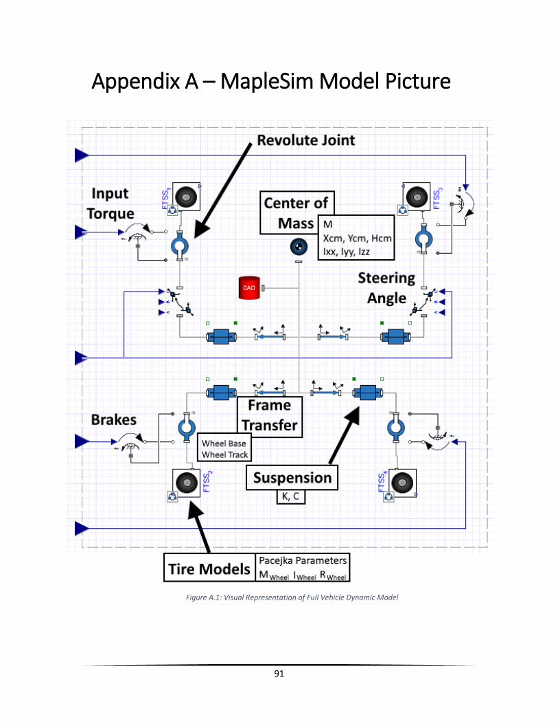
91
Appendix A – MapleSim Model Picture
Figure A.1: Visual Representation of Full Vehicle Dynamic Model

92
Figure A.2: Schematic of the Full Vehicle Dynamic Model
Note that the suspension trajectory is not purely vertical, it is represented by the spline outlined in Section
3.2.4.3. In summary, as the suspension compresses and extends, the camber angle changes slightly.

93
Appendix B – Final Parameter Values
PARAMETER INITIAL VALUE FINAL VALUE DESCRIPTION
M 2202 [kg] 2202 [kg] Mass of the vehicle with VMS attached
𝑿𝑪𝑴 1.39 [m] 1.35 [m] Perpendicular distance from the center of mass to the front axle
𝒀𝑪𝑴 0.865 [m] 0.833 [m] Perpendicular distance from the center of mass to the center of the front left wheel
𝑯𝑪𝑴 0.566 [m] 0.542 [m] Distance from the center of mass to the ground
WHEEL BASE 2.85 [m] 2.85 [m] Distance from the front axle to the rear axle
FRONT TRACK 1.582 [m] 1.582 [m] Distance from the center line of the front left wheel to the center line of the front right wheel
REAR TRACK 1.575 [m] 1.575 [m] Distance from the center line of the rear left wheel to the center line of the rear right wheel
𝑴𝑾𝒉𝒆𝒆𝒍 14.7 [kg] 14.7 [kg] Mass of the wheel with WFS rims
𝑰𝒀𝒀𝑾𝒉𝒆𝒆𝒍 1.40 [kg m2] 1.38 [kg m2] Principle moment of inertia about the spin
axis of the wheel 𝑹𝑾𝒉𝒆𝒆𝒍 0.34 [m] 0.34 [m] Unloaded radius of the tires
𝑰𝑿𝑿 1786 [kg m2] 1840 [kg m2] Principle moment of inertia about the x-axis (Roll Inertia)
𝑰𝒀𝒀 3712 [kg m2] 3700 [kg m2] Principle moment of inertia about the y-axis (Pitch Inertia)
𝑰𝒁𝒁 4197 [kg m2] 4220 [kg m2] Principle moment of inertia about the z-axis (Yaw Inertia)
𝑨𝑭 2.08 [m2] 2.23 [m2] Frontal area of the vehicle
𝝆 1.2 [kg m3] 1.2 [kg m3] Density of air
𝑪𝑫 0.743 0.59 Coefficient of drag
𝝁𝑹 0.0101 0.012 Coefficient of rolling resistance
𝑪�̇�>𝟎 26300 [Ns/m] 26300 [Ns/m] Damping coefficient while suspension velocity > 0
𝑪�̇�<𝟎 68600 [Ns/m] 68600 [Ns/m] Damping coefficient while suspension velocity < 0
Table B.1: Final parameter values for the Moose
Note that the spring stiffness is represented by Equation 3.25, where x is the compression of the spring.
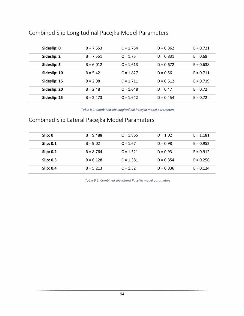
94
Combined Slip Longitudinal Pacejka Model Parameters
Sideslip: 0 B = 7.553 C = 1.754 D = 0.862 E = 0.721
Sideslip: 2 B = 7.551 C = 1.75 D = 0.831 E = 0.68
Sideslip: 5 B = 6.012 C = 1.613 D = 0.672 E = 0.638
Sideslip: 10 B = 5.42 C = 1.827 D = 0.56 E = 0.711
Sideslip: 15 B = 2.98 C = 1.711 D = 0.512 E = 0.719
Sideslip: 20 B = 2.48 C = 1.648 D = 0.47 E = 0.72
Sideslip: 25 B = 2.473 C = 1.642 D = 0.454 E = 0.72
Table B.2: Combined slip longitudinal Pacejka model parameters
Combined Slip Lateral Pacejka Model Parameters
Slip: 0 B = 9.488 C = 1.865 D = 1.02 E = 1.181
Slip: 0.1 B = 9.02 C = 1.67 D = 0.98 E = 0.952
Slip: 0.2 B = 8.764 C = 1.521 D = 0.93 E = 0.912
Slip: 0.3 B = 6.128 C = 1.381 D = 0.854 E = 0.256
Slip: 0.4 B = 5.213 C = 1.32 D = 0.836 E = 0.124
Table B.3: Combined slip lateral Pacejka model parameters