Theory of cortical plasticity in visionbyGeorge J. KalarickalA dissertation submitted to the faculty of the University of North Carolina at Chapel Hillin partial ful�llment of the requirements for the degree of Doctor of Philosophy in theDepartment of Computer Science. Chapel Hill1998Approved by:Prof. Jonathan A. Marshall, AdvisorDr. William D. Ross, ReaderProf. Oleg V. Favorov, ReaderProf. David FitzpatrickProf. Stephen M. Pizer

ii

c 1998George J. KalarickalALL RIGHTS RESERVED

iii

To Wg. Cdr. and Mrs. K.J. Joseph and Fr. Sebastian Kalarickal, S.J.

ivGeorge J. Kalarickal. Theory of cortical plasticity in vision(Under the direction of Professor Jonathan A. Marshall.)ABSTRACTA theory of postnatal activity-dependent neural plasticity based on synapticweight modi�cation is presented. Synaptic weight modi�cations are governed by simplevariants of a Hebbian rule for excitatory pathways and an anti-Hebbian rule for inhibitorypathways. The dissertation focuses on modeling the following cortical phenomena:long-term potentiation and depression (LTP and LTD); dynamic receptive �eld changesduring arti�cial scotoma conditioning in adult animals; adult cortical plasticity induced bybilateral retinal lesions, intracortical microstimulation (ICMS), and repetitive peripheralstimulation; changes in ocular dominance during \classical" rearing conditioning; and thee�ect of neuropharmacological manipulations on plasticity. Novel experiments are proposedto test the predictions of the proposed models, and the models are compared with othermodels of cortical properties.The models presented in the dissertation provide insights into the neural basisof perceptual learning . In perceptual learning, persistent changes in cortical neuronalreceptive �elds are produced by conditioning procedures that manipulate the activationof cortical neurons by repeated activation of localized cortical regions. Thus, the analysis ofsynaptic plasticity rules for receptive �eld changes produced by conditioning procedures thatactivate small groups of neurons can also elucidate the neural basis of perceptual learning.Previous experimental and theoretical work on cortical plasticity focused mainlyon a�erent excitatory synaptic plasticity. The novel and unifying theme in this work isself-organization and the use of the lateral inhibitory synaptic plasticity rule. Many corticalproperties, e.g., orientation selectivity, motion selectivity, spatial frequency selectivity, etc.are produced or strongly in uenced by inhibitory interactions. Thus, changes in theseproperties could be produced by lateral inhibitory synaptic plasticity.

vAcknowledgementsI thank Dr. Jonathan Marshall for his guidance, advice, and support during my �ve yearsat UNC-Chapel Hill. I immensely enjoyed working with Dr. Marshall. I am grateful tohim for imparting to me his good taste for relevant and important research work and forteaching me the art of identifying important research questions. I appreciate his help inimproving my writing and public speaking skills.I am grateful for the encouragement and the support from Dr. Stephen Pizer,Dr. David Fitzpatrick, Dr. Oleg Favorov, and Dr. William Ross. I appreciate their adviceand critical review of my work. I am thankful to Dr. Nestor Schmajuk for initially servingon my dissertation committee. I was very lucky to have Dr. Oleg Favorov join the committeeat very short notice. I thank Dr. Favorov and Dr. Ross for reading my dissertation.I thank Richard Alley, Vinay Gupta, Charles Schmitt, and Viswanath Srikanthfor their help, advice, and support. I am grateful to all in the Department of ComputerScience for making it a fun and happy place to work.This work was supported in part by the O�ce of Naval Research (Cognitive andNeural Sciences) and by the Whitaker Foundation (Special Opportunity Grant).

viContentsList of Figures xiList of Tables xvii1 Introduction: Motivation and overview 11.1 Introduction : : : : : : : : : : : : : : : : : : : : : : : : : : : : : : : : : : : : 11.2 Simpli�ed neural circuit : : : : : : : : : : : : : : : : : : : : : : : : : : : : : 51.3 Plasticity in early postnatal and adult cortex : : : : : : : : : : : : : : : : : 71.3.1 Long-term synaptic plasticity : : : : : : : : : : : : : : : : : : : : : : 101.3.2 Cortical plasticity in early postnatal development : : : : : : : : : : : 121.3.3 Cortical plasticity during pharmacological infusions : : : : : : : : : : 131.3.4 Cortical plasticity induced by peripheral conditioning : : : : : : : : 141.3.5 Cortical plasticity induced by intracortical microstimulation : : : : : 151.4 The rules of long-term synaptic plasticity : : : : : : : : : : : : : : : : : : : 151.5 Relation to previous theories : : : : : : : : : : : : : : : : : : : : : : : : : : 181.6 Emphasis on lateral inhibitory interactions : : : : : : : : : : : : : : : : : : 191.7 Thesis statement : : : : : : : : : : : : : : : : : : : : : : : : : : : : : : : : : 211.8 Overall contributions and signi�cance : : : : : : : : : : : : : : : : : : : : : 211.9 Outline of the dissertation : : : : : : : : : : : : : : : : : : : : : : : : : : : : 222 Comparison of generalized Hebbian rules for long-term synaptic plasticity 252.1 Introduction : : : : : : : : : : : : : : : : : : : : : : : : : : : : : : : : : : : : 262.2 Methods : : : : : : : : : : : : : : : : : : : : : : : : : : : : : : : : : : : : : : 292.2.1 The activation equation : : : : : : : : : : : : : : : : : : : : : : : : : 302.2.2 Synaptic plasticity rules : : : : : : : : : : : : : : : : : : : : : : : : : 312.3 Results : : : : : : : : : : : : : : : : : : : : : : : : : : : : : : : : : : : : : : : 342.3.1 Analyses of excitatory synaptic plasticity rules : : : : : : : : : : : : 352.3.2 Analysis of the outstar lateral inhibitory synaptic plasticity rule : : 452.3.3 Characteristics of the excitatory synaptic plasticity rules : : : : : : : 462.3.4 Combined e�ects of instar and outstar excitatory synaptic plasticityrules : : : : : : : : : : : : : : : : : : : : : : : : : : : : : : : : : : : : 752.3.5 Characteristics of the outstar inhibitory synaptic plasticity rule : : : 792.4 Discussion : : : : : : : : : : : : : : : : : : : : : : : : : : : : : : : : : : : : : 86

vii2.4.1 Experimental evidence for the excitatory synaptic plasticity rules : : 902.4.2 Experimental evidence for the outstar lateral inhibitory synapticplasticity rule : : : : : : : : : : : : : : : : : : : : : : : : : : : : : : : 1112.4.3 Functional signi�cance of the synaptic plasticity rules : : : : : : : : 1142.4.4 Comparison of the functional roles of the instar and outstar excitatoryrules : : : : : : : : : : : : : : : : : : : : : : : : : : : : : : : : : : : : 1192.4.5 Conclusions : : : : : : : : : : : : : : : : : : : : : : : : : : : : : : : : 1223 The role of a�erent excitatory and lateral inhibitory synaptic plasticityin visual cortical ocular dominance plasticity 1243.1 Introduction : : : : : : : : : : : : : : : : : : : : : : : : : : : : : : : : : : : : 1253.2 Methods : : : : : : : : : : : : : : : : : : : : : : : : : : : : : : : : : : : : : : 1283.2.1 EXIN model of ocular dominance shifts : : : : : : : : : : : : : : : : 1283.2.2 Initial network structure : : : : : : : : : : : : : : : : : : : : : : : : : 1313.2.3 Measures of cortical properties : : : : : : : : : : : : : : : : : : : : : 1313.3 Results : : : : : : : : : : : : : : : : : : : : : : : : : : : : : : : : : : : : : : : 1323.3.1 Normal rearing : : : : : : : : : : : : : : : : : : : : : : : : : : : : : : 1323.3.2 Monocular deprivation : : : : : : : : : : : : : : : : : : : : : : : : : : 1383.3.3 Reverse suture : : : : : : : : : : : : : : : : : : : : : : : : : : : : : : 1413.3.4 Strabismus : : : : : : : : : : : : : : : : : : : : : : : : : : : : : : : : 1453.3.5 Binocular deprivation : : : : : : : : : : : : : : : : : : : : : : : : : : 1453.3.6 Recovery : : : : : : : : : : : : : : : : : : : : : : : : : : : : : : : : : 1463.4 Discussion : : : : : : : : : : : : : : : : : : : : : : : : : : : : : : : : : : : : : 1513.4.1 Role of lateral inhibitory synaptic plasticity on neuronal featureselectivity : : : : : : : : : : : : : : : : : : : : : : : : : : : : : : : : : 1583.4.2 Site of cortical OD plasticity : : : : : : : : : : : : : : : : : : : : : : 1603.4.3 Comparison with other models of cortical OD plasticity : : : : : : : 1604 Plasticity in cortical neuron properties: Modeling the e�ects of an NMDAantagonist and a GABA agonist during visual deprivation 1634.1 Introduction : : : : : : : : : : : : : : : : : : : : : : : : : : : : : : : : : : : : 1644.1.1 Disruption of MD by pharmacological infusion : : : : : : : : : : : : 1654.1.2 Aspeci�c e�ects of infusion of APV and muscimol : : : : : : : : : : 1664.1.3 Previous models : : : : : : : : : : : : : : : : : : : : : : : : : : : : : 1664.1.4 Signi�cance and contributions of the chapter : : : : : : : : : : : : : 1674.2 EXIN model of changes in cortical properties : : : : : : : : : : : : : : : : : 1704.2.1 The EXIN plasticity rules : : : : : : : : : : : : : : : : : : : : : : : : 1704.2.2 The activation rule : : : : : : : : : : : : : : : : : : : : : : : : : : : : 1724.2.3 Explanation based on the EXIN plasticity rules : : : : : : : : : : : : 1734.3 Methods : : : : : : : : : : : : : : : : : : : : : : : : : : : : : : : : : : : : : : 1754.3.1 Initial network structure : : : : : : : : : : : : : : : : : : : : : : : : : 1754.3.2 Pharmacological manipulations : : : : : : : : : : : : : : : : : : : : : 1754.3.3 Simulation procedure : : : : : : : : : : : : : : : : : : : : : : : : : : 1764.3.4 Measures of cortical properties : : : : : : : : : : : : : : : : : : : : : 1764.4 Results : : : : : : : : : : : : : : : : : : : : : : : : : : : : : : : : : : : : : : : 177

viii4.4.1 Aspeci�c e�ects of pharmacological treatments : : : : : : : : : : : : 1784.4.2 E�ects of pharmacological treatments during MD : : : : : : : : : : : 1794.4.3 Important model parameters : : : : : : : : : : : : : : : : : : : : : : 1884.5 Discussion : : : : : : : : : : : : : : : : : : : : : : : : : : : : : : : : : : : : : 1944.5.1 Loss of cortical neuronal stimulus feature selectivity : : : : : : : : : 1954.5.2 Model predictions : : : : : : : : : : : : : : : : : : : : : : : : : : : : 1964.5.3 Conclusions : : : : : : : : : : : : : : : : : : : : : : : : : : : : : : : : 2005 Models of receptive �eld dynamics in visual cortex 2015.1 Introduction : : : : : : : : : : : : : : : : : : : : : : : : : : : : : : : : : : : : 2025.1.1 Signi�cance of RF dynamics : : : : : : : : : : : : : : : : : : : : : : : 2045.1.2 Modeling of RF dynamics : : : : : : : : : : : : : : : : : : : : : : : : 2055.1.3 Signi�cance and contributions of this chapter : : : : : : : : : : : : : 2085.2 Methods : : : : : : : : : : : : : : : : : : : : : : : : : : : : : : : : : : : : : : 2105.2.1 Network simulation organization : : : : : : : : : : : : : : : : : : : : 2105.2.2 The inputs : : : : : : : : : : : : : : : : : : : : : : : : : : : : : : : : 2115.2.3 Simulation procedure : : : : : : : : : : : : : : : : : : : : : : : : : : 2125.2.4 RF measurements : : : : : : : : : : : : : : : : : : : : : : : : : : : : 2125.2.5 The EXIN model : : : : : : : : : : : : : : : : : : : : : : : : : : : : : 2125.2.6 The LISSOM model : : : : : : : : : : : : : : : : : : : : : : : : : : : 2225.2.7 The inhibition-dominant adaptation model : : : : : : : : : : : : : : 2305.2.8 The adaptation model with no lateral interaction : : : : : : : : : : : 2345.2.9 The excitation-dominant adaptation model : : : : : : : : : : : : : : 2345.3 Simulation results: Scotoma stimuli : : : : : : : : : : : : : : : : : : : : : : : 2355.3.1 Comparison of outstar/instar lateral inhibitory synaptic plasticityrules and neuronal adaptation : : : : : : : : : : : : : : : : : : : : : : 2365.3.2 Role of a�erent excitatory synaptic plasticity : : : : : : : : : : : : : 2555.3.3 Role of lateral excitatory synaptic plasticity : : : : : : : : : : : : : : 2645.4 Simulation results: Complementary scotoma stimuli : : : : : : : : : : : : : : 2685.4.1 RF changes because of synaptic plasticity : : : : : : : : : : : : : : : 2685.4.2 RF changes because of neuronal adaptation : : : : : : : : : : : : : : 2725.4.3 Recovery of RF properties : : : : : : : : : : : : : : : : : : : : : : : : 2785.4.4 Conclusions : : : : : : : : : : : : : : : : : : : : : : : : : : : : : : : : 2785.5 Discussion : : : : : : : : : : : : : : : : : : : : : : : : : : : : : : : : : : : : : 2795.5.1 Models based on the EXIN and the LISSOM rules : : : : : : : : : : 2855.5.2 Transient response bias in RF measurements : : : : : : : : : : : : : 2865.5.3 E�ect of orientation on RF dynamics : : : : : : : : : : : : : : : : : : 2865.5.4 Long-term e�ects of retinal lesions on RF properties : : : : : : : : : 2875.5.5 Role of lateral excitatory pathways in RF properties : : : : : : : : : 2885.5.6 Signi�cance of the EXIN lateral inhibitory plasticity rule : : : : : : 2895.5.7 Neurophysiological realization of the EXIN lateral inhibitoryplasticity rule : : : : : : : : : : : : : : : : : : : : : : : : : : : : : : : 2915.5.8 Conclusions : : : : : : : : : : : : : : : : : : : : : : : : : : : : : : : : 293

ix6 Rearrangement of receptive �eld topography after intracortical andperipheral stimulation: The role of plasticity in inhibitory pathways 2946.1 Introduction : : : : : : : : : : : : : : : : : : : : : : : : : : : : : : : : : : : : 2956.1.1 Cortical plasticity in adult animals : : : : : : : : : : : : : : : : : : : 2956.1.2 Receptive �eld topography changes after intracortical microstimulation2976.1.3 Receptive �eld topography changes after peripheral stimulation : : : 2986.1.4 Previously suggested mechanisms : : : : : : : : : : : : : : : : : : : : 2986.1.5 EXIN model of RF changes : : : : : : : : : : : : : : : : : : : : : : : 3016.1.6 Signi�cance and contributions of the chapter : : : : : : : : : : : : : 3026.2 Methods : : : : : : : : : : : : : : : : : : : : : : : : : : : : : : : : : : : : : : 3026.2.1 Model architecture : : : : : : : : : : : : : : : : : : : : : : : : : : : : 3046.2.2 Model stimulation procedures : : : : : : : : : : : : : : : : : : : : : : 3046.2.3 Simulation procedure : : : : : : : : : : : : : : : : : : : : : : : : : : 3076.2.4 RF measurements : : : : : : : : : : : : : : : : : : : : : : : : : : : : 3086.2.5 The EXIN model : : : : : : : : : : : : : : : : : : : : : : : : : : : : : 3096.3 Simulation results : : : : : : : : : : : : : : : : : : : : : : : : : : : : : : : : 3156.3.1 The e�ects of ICMS on the model : : : : : : : : : : : : : : : : : : : 3166.3.2 The e�ects of model ICMS parameters : : : : : : : : : : : : : : : : : 3326.3.3 The e�ects of RF scatter during ICMS : : : : : : : : : : : : : : : : : 3586.3.4 The e�ects of peripheral stimulation : : : : : : : : : : : : : : : : : : 3586.3.5 Changes in stimulus discrimination after peripheral stimulation : : : 3646.4 Discussion : : : : : : : : : : : : : : : : : : : : : : : : : : : : : : : : : : : : : 3726.4.1 Explanation of the RF changes during ICMS and peripheral stimulation3746.4.2 Stability of EXIN networks : : : : : : : : : : : : : : : : : : : : : : : 3776.4.3 Assumptions of the model : : : : : : : : : : : : : : : : : : : : : : : : 3786.4.4 Signi�cance of lateral inhibitory plasticity : : : : : : : : : : : : : : : 3816.4.5 Model predictions : : : : : : : : : : : : : : : : : : : : : : : : : : : : 3836.4.6 Neurophysiological realization of the EXIN synaptic plasticity rules : 3867 Conclusions and future work 3887.1 Summary : : : : : : : : : : : : : : : : : : : : : : : : : : : : : : : : : : : : : 3907.2 Future work : : : : : : : : : : : : : : : : : : : : : : : : : : : : : : : : : : : : 3927.2.1 Development of topographic cortical maps : : : : : : : : : : : : : : : 3937.2.2 Neural basis of perceptual learning : : : : : : : : : : : : : : : : : : : 3957.2.3 Changes in information content of self-organizing networks afterchanges in input environment : : : : : : : : : : : : : : : : : : : : : : 3967.2.4 Self-organization of stereopsis : : : : : : : : : : : : : : : : : : : : : : 3967.2.5 Binocular rivalry : : : : : : : : : : : : : : : : : : : : : : : : : : : : : 397A Parameters used in the simulations of Chapter 2 400B Parameters used in the simulations of Chapters 3 and 4 406B.1 Activation equation parameters : : : : : : : : : : : : : : : : : : : : : : : : : 406B.2 Initial network : : : : : : : : : : : : : : : : : : : : : : : : : : : : : : : : : : 406B.3 Training and test stimuli : : : : : : : : : : : : : : : : : : : : : : : : : : : : : 407

xB.4 Normal rearing procedure : : : : : : : : : : : : : : : : : : : : : : : : : : : : 408B.5 Classical rearing manipulations : : : : : : : : : : : : : : : : : : : : : : : : : 409B.6 Parameters for synaptic plasticity rules : : : : : : : : : : : : : : : : : : : : : 410B.7 Parameters for aspeci�c action of pharmacological infusion : : : : : : : : : : 410B.8 E�ects of pharmacological infusion : : : : : : : : : : : : : : : : : : : : : : : 410B.8.1 APV infusion : : : : : : : : : : : : : : : : : : : : : : : : : : : : : : : 411B.8.2 Muscimol infusion : : : : : : : : : : : : : : : : : : : : : : : : : : : : 411C Parameters used in the simulations of Chapter 5 412C.1 Parameters for the EXIN model simulations : : : : : : : : : : : : : : : : : : 412C.1.1 Parameters for the activation equation : : : : : : : : : : : : : : : : : 413C.1.2 Parameters for the learning equations : : : : : : : : : : : : : : : : : 415C.2 Parameters for the LISSOM simulations : : : : : : : : : : : : : : : : : : : : 419C.2.1 Parameters for the activation equation : : : : : : : : : : : : : : : : : 419C.2.2 Parameters for the learning equations : : : : : : : : : : : : : : : : : 419C.3 Parameters for the adaptation model simulations : : : : : : : : : : : : : : : 420C.3.1 Parameters for the activation equation : : : : : : : : : : : : : : : : : 421C.3.2 Parameters for the adaptation equation : : : : : : : : : : : : : : : : 421C.4 Parameters for generating the inputs for the simulations : : : : : : : : : : : 422C.5 Parameters for RF measurements : : : : : : : : : : : : : : : : : : : : : : : : 422C.6 Conditioning procedure : : : : : : : : : : : : : : : : : : : : : : : : : : : : : 422D Parameters used in the simulations of Chapter 6 424D.1 Parameters for the activation equation : : : : : : : : : : : : : : : : : : : : : 424D.2 Parameters for initial synaptic strength values : : : : : : : : : : : : : : : : : 425D.3 Parameters for the initial training phase : : : : : : : : : : : : : : : : : : : : 426D.4 Parameters for ICMS simulations : : : : : : : : : : : : : : : : : : : : : : : : 427D.4.1 ICMS simulations in Section 6.3.1 : : : : : : : : : : : : : : : : : : : 427D.4.2 ICMS simulations in Section 6.3.2 : : : : : : : : : : : : : : : : : : : 427D.4.3 ICMS simulations in Section 6.3.3 : : : : : : : : : : : : : : : : : : : 428D.5 Parameters for peripheral stimulation simulations : : : : : : : : : : : : : : : 428D.6 Parameters for RF measurements : : : : : : : : : : : : : : : : : : : : : : : : 429Bibliography 430

xiList of Figures1.1 Pathway connection pattern in the primary visual cortex. : : : : : 81.2 Simpli�ed neural circuit. : : : : : : : : : : : : : : : : : : : : : : : : : : 91.3 Abstract neural circuit. : : : : : : : : : : : : : : : : : : : : : : : : : : : 101.4 Experimental con�guration for experiments on long-term synapticplasticity. : : : : : : : : : : : : : : : : : : : : : : : : : : : : : : : : : : : : 111.5 Comparison of instar and outstar plasticity rules. : : : : : : : : : : : 172.1 The BCM excitatory synaptic plasticity rule. : : : : : : : : : : : : : 372.2 The BCM excitatory synaptic plasticity rule. : : : : : : : : : : : : : 382.3 Change in synaptic weight as a function of the postsynaptic activityusing the BCM rule. : : : : : : : : : : : : : : : : : : : : : : : : : : : : : 402.4 Change in synaptic weight as a function of the presynaptic activityusing the instar excitatory synaptic plasticity rule. : : : : : : : : : : 412.5 Change in synaptic weight as a function of the presynaptic activityusing the outstar excitatory synaptic plasticity rule. : : : : : : : : : 442.6 The outstar inhibitory synaptic plasticity rule under the linearityassumption. : : : : : : : : : : : : : : : : : : : : : : : : : : : : : : : : : : : 472.7 Model network. : : : : : : : : : : : : : : : : : : : : : : : : : : : : : : : : 492.8 Simulation results: Changes in excitatory synaptic e�cacy ofstimulated and unstimulated pathways as a function of presynapticstimulation strength. : : : : : : : : : : : : : : : : : : : : : : : : : : : : : 522.9 Simulation results: Changes in excitatory synaptic e�cacy ofstimulated and unstimulated pathways under faster learningparameters. : : : : : : : : : : : : : : : : : : : : : : : : : : : : : : : : : : : 542.10 Simulation results: Equilibrium values of excitatory synaptice�cacy of stimulated and unstimulated pathways. : : : : : : : : : : 582.11 Simulation results: Equilibrium values of excitatory synaptice�cacy of stimulated and unstimulated pathways according to theBCM rule. : : : : : : : : : : : : : : : : : : : : : : : : : : : : : : : : : : : : 602.12 Simulation results: The e�ects of lateral inhibitory weight onexcitatory synaptic plasticity. : : : : : : : : : : : : : : : : : : : : : : : : 622.13 Simulation results: Excitatory synaptic plasticity produced bystimulation of equally strong pathways to di�erent neurons. : : : : 64

xii2.14 Simulation results: Changes in excitatory synaptic e�cacy of thestimulated pathway as a function of postsynaptic activation. : : : : 662.15 Simulation results: Changes in excitatory synaptic e�cacy of thestimulated pathway as a function of initial synaptic e�cacy. : : : : 682.16 Simulation results: Changes in excitatory synaptic e�cacy of thestimulated pathway according to the BCM rule as a function ofprior presynaptic stimulation. : : : : : : : : : : : : : : : : : : : : : : : 702.17 Simulation results: Postsynaptic activation caused by stimulationof independent excitatory pathways. : : : : : : : : : : : : : : : : : : : 712.18 Simulation results: Associative synaptic plasticity. : : : : : : : : : : 732.19 Simulation results: Postsynaptic activation caused by stimulationof independent excitatory pathways in a network with asymmetriclateral inhibitory weights. : : : : : : : : : : : : : : : : : : : : : : : : : : 732.20 Simulation results: Associative synaptic plasticity in a networkwith asymmetric lateral inhibitory weights. : : : : : : : : : : : : : : : 752.21 Simulation results: Synaptic plasticity with �xed presynapticstimulation and variable postsynaptic activation level under theinstar and the outstar excitatory synaptic plasticity rules. : : : : : 782.22 Simulation results: Changes in inhibitory synaptic e�cacy underthe outstar inhibitory synaptic plasticity rule as a function of inputexcitation. : : : : : : : : : : : : : : : : : : : : : : : : : : : : : : : : : : : : 812.23 Simulation results: Changes in inhibitory synaptic e�cacy underthe outstar inhibitory synaptic plasticity rule produced by unequalactivation of neurons. : : : : : : : : : : : : : : : : : : : : : : : : : : : : : 832.24 Simulation results: Equilibrium value of inhibitory synaptice�cacy under the outstar inhibitory synaptic plasticity rule. : : : 852.25 Simulation results: Changes in inhibitory synaptic e�cacy underthe outstar inhibitory synaptic plasticity rule as a function ofpre- and postsynaptic activation. : : : : : : : : : : : : : : : : : : : : : 852.26 Simulation results: Changes in inhibitory synaptic e�cacy underthe outstar inhibitory synaptic plasticity rule as a function of initialinhibitory weight. : : : : : : : : : : : : : : : : : : : : : : : : : : : : : : : 872.27 Simulation results: Changes in inhibitory synaptic e�cacy underthe outstar inhibitory synaptic plasticity rule as reciprocalinhibitory weights were varied. : : : : : : : : : : : : : : : : : : : : : : : 882.28 Simulation results: Changes in inhibitory synaptic e�cacy underthe outstar inhibitory synaptic plasticity rule as reciprocal weightswere varied and the neurons received equal input excitations. : : : 893.1 Normal rearing. : : : : : : : : : : : : : : : : : : : : : : : : : : : : : : : : 1333.2 Development of monocular RFs during NR. : : : : : : : : : : : : : : 1343.3 NR with binocular inputs over a larger disparity range. : : : : : : : 1353.4 The e�ects of varying the inhibitory weights during NR. : : : : : : 1373.5 OD changes during MD. : : : : : : : : : : : : : : : : : : : : : : : : : : : 1393.6 Monocular RF changes during MD. : : : : : : : : : : : : : : : : : : : 140

xiii3.7 OD changes during RS. : : : : : : : : : : : : : : : : : : : : : : : : : : : 1413.8 Monocular RF changes during RS. : : : : : : : : : : : : : : : : : : : : 1423.9 Monocular RF changes during NR for the neurons in Figure 3.8. : 1433.10 OD changes during ST. : : : : : : : : : : : : : : : : : : : : : : : : : : : 1463.11 Monocular RF changes during ST. : : : : : : : : : : : : : : : : : : : : 1473.12 OD changes during BD. : : : : : : : : : : : : : : : : : : : : : : : : : : : 1483.13 Monocular RF changes during BD. : : : : : : : : : : : : : : : : : : : : 1493.14 Monocular RF changes during BD without lateral inhibitorysynaptic plasticity. : : : : : : : : : : : : : : : : : : : : : : : : : : : : : : : 1503.15 OD during RE following MD. : : : : : : : : : : : : : : : : : : : : : : : 1513.16 Monocular RF changes during RE following MD. : : : : : : : : : : : 1523.17 OD during RE following BD. : : : : : : : : : : : : : : : : : : : : : : : : 1533.18 Monocular RF changes during RE following BD. : : : : : : : : : : : 1543.19 Monocular RF changes during RE following prolonged BD andduring NR. : : : : : : : : : : : : : : : : : : : : : : : : : : : : : : : : : : : 1553.20 OD during RE following ST. : : : : : : : : : : : : : : : : : : : : : : : : 1563.21 Monocular RF changes during RE following ST. : : : : : : : : : : : 1574.1 Models OD changes. : : : : : : : : : : : : : : : : : : : : : : : : : : : : : 1694.2 Model OD distribution before MD. : : : : : : : : : : : : : : : : : : : : 1774.3 Aspeci�c e�ects of APV. : : : : : : : : : : : : : : : : : : : : : : : : : : 1804.4 Aspeci�c e�ects of APV with lateral inhibitory plasticity. : : : : : 1814.5 Aspeci�c e�ects of muscimol. : : : : : : : : : : : : : : : : : : : : : : : : 1824.6 Aspeci�c e�ects of muscimol with a�erent excitatory and lateralinhibitory synaptic plasticity. : : : : : : : : : : : : : : : : : : : : : : : : 1834.7 Changes in RF properties after MD with APV infusion. : : : : : : 1844.8 Changes in RF properties after MD with APV infusion with lateralinhibitory pathway synaptic plasticity disabled. : : : : : : : : : : : : 1854.9 Model OD distribution after MD with muscimol infusion. : : : : : 1864.10 Model OD distribution after MD with muscimol infusion withlateral inhibitory pathway synaptic plasticity disabled. : : : : : : : 1874.11 Dependence of OD shifts on APV concentration. : : : : : : : : : : : 1894.12 Dependence of OD shifts on muscimol concentration. : : : : : : : : 1904.13 Dependence of RF width and responsiveness on cortical activation. 1924.14 RF width and responsiveness in the presence of APV or muscimol. 1945.1 Site of RF changes. : : : : : : : : : : : : : : : : : : : : : : : : : : : : : : 2065.2 Network architecture for the EXIN model. : : : : : : : : : : : : : : : 2145.3 The e�ects of scotoma conditioning on the EXIN model. : : : : : : 2195.4 Network architecture for the LISSOM model and theinhibition-dominant adaptation model. : : : : : : : : : : : : : : : : : : 2245.5 The e�ects of scotoma conditioning on the LISSOM model. : : : : 2285.6 The e�ects of scotoma conditioning on the inhibition-dominantadaptation model. : : : : : : : : : : : : : : : : : : : : : : : : : : : : : : : 2335.7 Simulation results: RF expansion and contraction. : : : : : : : : : : 239

xiv5.8 Simulation results: The iceberg e�ect. : : : : : : : : : : : : : : : : : : 2405.9 Simulation results: RF size as a function of position. : : : : : : : : 2425.10 Simulation results: Changes in RF after scotoma conditioning witha smaller scotoma. : : : : : : : : : : : : : : : : : : : : : : : : : : : : : : : 2435.11 Simulation results: Recovery of responsiveness of Layer 2 neurons. 2455.12 RF shift as function of position. : : : : : : : : : : : : : : : : : : : : : : 2475.13 Simulation results: Blank screen causes RF changes in theinhibition-dominant adaptation model. : : : : : : : : : : : : : : : : : : 2495.14 Simulation results: RF size changes in other adaptation models. : 2505.15 Simulation results: The iceberg e�ect in other adaptation models. 2515.16 Simulation results: RF shifts in other adaptation models. : : : : : 2525.17 Simulation results: Recovery of responsiveness in other adaptationmodels. : : : : : : : : : : : : : : : : : : : : : : : : : : : : : : : : : : : : : : 2535.18 Simulation results: RF size changes caused by a�erent excitatoryplasticity. : : : : : : : : : : : : : : : : : : : : : : : : : : : : : : : : : : : : 2565.19 Simulation results: RF pro�les of neurons that show expansion orcontraction. : : : : : : : : : : : : : : : : : : : : : : : : : : : : : : : : : : : 2585.20 Simulation results: Activation pro�les in response to inputs atlocations away from the scotoma. : : : : : : : : : : : : : : : : : : : : : 2595.21 Simulation results: Recovery of responsiveness of Layer 2 neuronscaused by a�erent excitatory plasticity. : : : : : : : : : : : : : : : : : 2605.22 Simulation results: RF shifts caused by a�erent excitatory plasticity.2625.23 Simulation results: RF changes in the LISSOM network with onlylateral excitatory plasticity enabled. : : : : : : : : : : : : : : : : : : : 2665.24 Simulation results: Average RF size changes after complementaryscotoma conditioning. : : : : : : : : : : : : : : : : : : : : : : : : : : : : 2705.25 Simulation results: Average RF size changes after complementaryscotoma conditioning. : : : : : : : : : : : : : : : : : : : : : : : : : : : : 2715.26 Simulation results: Average RF shifts after complementaryscotoma conditioning. : : : : : : : : : : : : : : : : : : : : : : : : : : : : 2735.27 Simulation results: Average RF shifts after complementaryscotoma conditioning. : : : : : : : : : : : : : : : : : : : : : : : : : : : : 2745.28 Simulation results: Average RF size changes after complementaryscotoma conditioning. : : : : : : : : : : : : : : : : : : : : : : : : : : : : 2755.29 Simulation results: Average RF shifts after complementaryscotoma conditioning. : : : : : : : : : : : : : : : : : : : : : : : : : : : : 2766.1 Network architecture of the EXIN model. : : : : : : : : : : : : : : : 3036.2 Intracortical microstimulation of model cortical layer. : : : : : : : : 3086.3 Spatial distribution of presynaptic excitation and postsynapticactivation. : : : : : : : : : : : : : : : : : : : : : : : : : : : : : : : : : : : : 3176.4 Changes in RF overlap with the ICMS-site RF. : : : : : : : : : : : : 3186.5 Changes in activation level of neurons caused by changes inthe distribution of presynaptic excitation to a�erent excitatorypathways. : : : : : : : : : : : : : : : : : : : : : : : : : : : : : : : : : : : : 319

xv6.6 Pre- and post-ICMS RFs. : : : : : : : : : : : : : : : : : : : : : : : : : : 3206.7 Pre- and post-ICMS a�erent excitatory and lateral inhibitorysynaptic weights. : : : : : : : : : : : : : : : : : : : : : : : : : : : : : : : : 3226.8 Changes in RF size. : : : : : : : : : : : : : : : : : : : : : : : : : : : : : : 3236.9 Changes in neuronal responsiveness after ICMS. : : : : : : : : : : : 3256.10 RF shift after ICMS. : : : : : : : : : : : : : : : : : : : : : : : : : : : : : 3266.11 Spatial distribution of changes in model cortical RF topography. : 3286.12 Temporal changes in RF topography and RF size during ICMS. : 3306.13 Temporal e�ects of ICMS on responsiveness. : : : : : : : : : : : : : : 3306.14 RF changes with additional ICMS. : : : : : : : : : : : : : : : : : : : : 3316.15 Changes pathway weights in ICMS simulations with a�erentexcitatory or lateral inhibitory synaptic plasticity disabled. : : : : 3346.16 Role of a�erent excitatory and lateral inhibitory plasticity inproducing RF changes. : : : : : : : : : : : : : : : : : : : : : : : : : : : : 3356.17 Changes in model cortical RF topography with only a�erentexcitatory plasticity. : : : : : : : : : : : : : : : : : : : : : : : : : : : : : 3366.18 E�ect of a�erent excitatory plasticity and lateral inhibitoryplasticity on responsiveness. : : : : : : : : : : : : : : : : : : : : : : : : 3376.19 Changes in model cortical RF topography with only lateralinhibitory plasticity. : : : : : : : : : : : : : : : : : : : : : : : : : : : : : : 3396.20 Synaptic plasticity in the simulation manipulating the magnitudeof presynaptic excitation to a�erent excitatory synapses producedby ICMS. : : : : : : : : : : : : : : : : : : : : : : : : : : : : : : : : : : : : 3406.21 Synaptic plasticity in the simulation manipulating the distributionof presynaptic excitation to a�erent excitatory synapses producedby ICMS. : : : : : : : : : : : : : : : : : : : : : : : : : : : : : : : : : : : : 3416.22 E�ects of the strength of presynaptic excitation of a�erentexcitatory pathways on model RF size and position. : : : : : : : : : 3436.23 E�ects of excitation strength of the presynaptic a�erent excitatorypathways on model responsiveness. : : : : : : : : : : : : : : : : : : : : 3446.24 E�ects of presynaptic stimulation distribution to the a�erentexcitatory pathways on model RF properties. : : : : : : : : : : : : : 3456.25 E�ects of presynaptic stimulation distribution to the a�erentexcitatory pathways on model responsiveness. : : : : : : : : : : : : : 3466.26 Changes in activation of model neurons caused by changes in thedistribution of direct excitation to the neurons. : : : : : : : : : : : : 3496.27 E�ects of distribution of direct stimulation to the model corticalneurons on RF properties. : : : : : : : : : : : : : : : : : : : : : : : : : 3506.28 E�ects of distribution of direct stimulation to the model corticalneurons on responsiveness. : : : : : : : : : : : : : : : : : : : : : : : : : 3516.29 Changes in activation of model neurons caused by changes in thedistribution of presynaptic excitation to lateral inhibitory pathways.352

xvi6.30 E�ects of distribution of presynaptic stimulation of lateralinhibitory pathways during ICMS on model RF topography andRF size. : : : : : : : : : : : : : : : : : : : : : : : : : : : : : : : : : : : : : 3536.31 E�ects of distribution of presynaptic stimulation of lateralinhibitory pathways during ICMS on model responsiveness. : : : : 3546.32 E�ects of distribution of presynaptic stimulation of lateralinhibitory pathways during ICMS on model RF topography andRF size. : : : : : : : : : : : : : : : : : : : : : : : : : : : : : : : : : : : : : 3556.33 E�ects of distribution of presynaptic stimulation of lateralinhibitory pathways during ICMS on model responsiveness. : : : : 3566.34 Initial model cortical RF topography in the scatter simulation. : : 3596.35 Changes in RF topography after ICMS in a network with RF scatter.3606.36 Changes in RF properties in a model network with RF scatter. : : 3616.37 Changes in responsiveness in a model network with RF scatter. : 3626.38 Spatial distribution of presynaptic excitation and postsynapticactivation in model during peripheral stimulation. : : : : : : : : : : 3646.39 Changes in activation of model neurons caused by variations inperipheral stimulation strength. : : : : : : : : : : : : : : : : : : : : : : 3656.40 Changes in model RF properties caused by peripheral stimulation. 3676.41 Changes in model neuron responsiveness caused by peripheralstimulation. : : : : : : : : : : : : : : : : : : : : : : : : : : : : : : : : : : : 3676.42 Changes in model cortical magni�cation caused by peripheralstimulation. : : : : : : : : : : : : : : : : : : : : : : : : : : : : : : : : : : : 3686.43 Changes in position discrimination after peripheral stimulation. : 369A.1 The e�ects of parameters A, B, and C on the activation equation. 403A.2 The e�ects of varying �, , input excitation function, and inputinhibition function on the activation equation. : : : : : : : : : : : : : 405C.1 Behavior of the EXIN network as a function of activation equationparameters. : : : : : : : : : : : : : : : : : : : : : : : : : : : : : : : : : : : 415C.2 Activation curves in the EXIN network after whole-�eld stimulation.416C.3 Stability of the EXIN network with lateral inhibitory synapticplasticity alone. : : : : : : : : : : : : : : : : : : : : : : : : : : : : : : : : 418D.1 Activation curves in the EXIN network after ICMS. : : : : : : : : : 425

xviiList of Tables2.1 Properties of the excitatory synaptic plasticity rules that areconsistent with experimental data. : : : : : : : : : : : : : : : : : : : : 922.2 Properties of the excitatory synaptic plasticity rules that areinconsistent with experimental data. : : : : : : : : : : : : : : : : : : : 932.3 Comparison of the excitatory synaptic plasticity rules. : : : : : : : 945.1 Comparison of models of dynamic RF changes : : : : : : : : : : : : : 280

Chapter 1Introduction: Motivation andoverview1.1 IntroductionThe visual system, even in adult animals, is highly plastic, i.e., easily modi�able.The perception of a visual feature depends on the surrounding (contextual) visual features inspace (simultaneously presented neighboring stimuli) and in time (e.g., previously presentedstimuli). For example, adaptation (from continuous viewing of a stimulus for few minutes)to a stimulus produces a contextual, orientation speci�c contrast threshold elevation for teststimuli (Blakemore & Nachmias, 1971). Adaptation e�ects are not persistent; they wearo� within a few minutes in the absence of visual stimulation. Adaptation to orientationstimuli can distort perception of test stimuli. In the tilt aftere�ect, after viewing a gratingof a particular orientation (e.g., vertical), an observer perceives o�-vertical gratings tobe more tilted away from the vertical than the actual test grating (Mayo et al., 1968).The response properties of neurons in the primary visual cortex, the �rst visual corticalprocessing stage, fatigue/adapt after the conditioning phase (Ma�ei & Fiorentini, 1973;Movshon & Lennie, 1979), and the neural adaptation is consistent with the tilt aftere�ect(see Sekuler & Blake, 1994, pp. 135).

2Prior viewing of stimuli over a longer period can also produce persistent changesin visual perception. For example, in perceptual learning , human observers improve theirperformance in perceptual tasks such as orientation perception (Fiorentini & Berardi, 1980),vernier acuity (Fahle & Edelman, 1993), and discrimination of texture (Karni & Sagi, 1991)after training. Perceptual learning is stable, as it does not wear o� after periods withoutvisual stimulation, unlike the adaptation e�ects. The e�ects of perceptual learning arevery speci�c; the improvement may be restricted to the orientation (Fahle et al., 1995;Poggio et al., 1992) and visual �eld position (Fahle et al., 1995; Karni & Sagi, 1991;Poggio et al., 1992) of the training stimuli. The e�ects of perceptual learning can be maskedby adaptation/fatigue. Improvement in perceptual performance may not be apparentduring training, but may manifest itself following a rest period during which the e�ectsof adaptation/fatigue dissipate (Fahle, 1997; Karni & Sagi, 1991).It has been proposed that the long-range lateral pathways in the primaryvisual cortex may subserve the e�ects of contextual stimuli and visual plasticity.The lateral long-range pathways in the primary visual cortex connect neurons withnon-overlapping \classical" receptive �elds, but with similar stimulus feature preferences,e.g., orientation (Gilbert & Wiesel, 1989; Weliky et al., 1995). Thus, neural representationsof distant visual stimuli may interact via the long-range pathways to produce the contextuale�ects. The receptive �eld properties of primary visual cortical neurons are a�ected bysimultaneously presented contextual stimuli (Gilbert & Wiesel, 1990; Sengpiel et al., 1997;Toth et al., 1996). Repeated presentation of stimuli used to characterize the e�ects ofneighboring stimuli on orientation preference of a neuron produced persistent changesin its orientation tuning (Gilbert & Wiesel, 1990). Karni and Sagi (1991) suggestedthat perceptual learning occurs even at the monocular stage of visual cortical processing.Herzog and Fahle (1995) suggested that perceptual learning may involve reciprocalinteractions among several visual cortical processing stages.Perceptual learning occurs in other sensory modalities too. For example,monkeys gradually improved their performance of a tactile frequency discriminationtask during several weeks of training (Recanzone et al., 1992a). The training alsoproduced changes in the receptive �eld properties of neurons in the somatosensory cortex

3(Recanzone et al., 1992acde).From an information theoretic viewpoint, animal brains adapt during long-termdevelopment and during short-term conditionings to maximize the information content ofneural signals (Atick & Redlich, 1990). Following changes in living environment, loss ofsensory organs (e.g., damage to retina, loss of limbs, etc.), or brain damage (e.g., fromstroke) the brain adapts to maximize the information content of its remaining capacitieswith respect to the new condition.An information-theoretic analysis of brain adaptation does not reveal the brainprocesses or the rules by which the brain adapts, although it constrains plausible rules forplasticity. Knowledge of the substrate(s) and the rules for brain adaptation is useful forclinical applications, e.g., treatment of brain damage, or recovery from loss of sense organs,as well as for design of arti�cial systems capable of mimicking animal brain functions,e.g., face recognition systems. The information theoretic approach does not elucidate themechanistic processes of the brain.Current psychophysical and neurobiological data suggest that corticalplasticity can be produced by changes in e�cacy of individual synapses (synapticplasticity) (Kirkwood et al., 1993), by habituation of individual synapses (synaptichabituation/adaptation) or in individual neurons (neuronal habituation/adaptation)(Movshon & Lennie, 1979; Varela et al., 1997), and by changes in axonal arborizationand synaptogenesis (Darian-Smith & Gilbert, 1994). Changes in these sites di�er in theirpersistence/stability and in the time scales at which they occur. Synaptic and neuronalhabituation are short-term changes; they are induced within a few seconds by synapticactivity and neuronal activity, respectively, and last for a few seconds after removal of theactivation. Synaptic plasticity depends on activation in pre- and postsynaptic elements; itis produced in several minutes and lasts for several tens of minutes. Changes in axonalarborization and synaptogenesis take several months and last for several months.In this dissertation, simple synaptic plasticity rules are used to model persistentchanges in receptive �eld properties of cortical neurons that are produced by conditioningprocedures that selectively activate a�erent pathways to cortical neurons, manipulate theactivation of cortical neurons, and produce activation in localized cortical regions. In

4perceptual learning, a stimulus con�guration is repeatedly presented. It is assumed that theneurons selective for the features of the training stimuli become repeatedly activated. Thus,the analysis of synaptic plasticity rules for receptive �eld changes produced by conditioningprocedures that activate small groups of neurons can shed light on the neural basis ofperceptual learning.The synaptic plasticity rules are compared with experimental data on synapticplasticity in the cortex and the hippocampus, and the rules are used to model severalphenomena of cortical plasticity in early postnatal and adult animals. Several corticalplasticity phenomenona are characterized as the emergent properties of a small set ofsynaptic plasticity rules. In particular, the EXIN rules (Marshall, 1995a; Marshall &Gupta, 1998), which comprise a Hebbian a�erent excitatory synaptic plasticity rule andan anti-Hebbian lateral inhibitory synaptic plasticity rule, are used to model� long-term potentiation (LTP) and long-term depression (LTD);� changes in ocular dominance during \classical" rearing conditioning;� changes in ocular dominance during visual deprivation with cortical infusion ofpharmacological agents;� dynamic receptive �eld (RF) changes during arti�cial scotoma conditioning and retinallesions;� changes in RF topography and RF properties after intracortical microstimulation; and� changes in RF topography and stimulus discrimination following repeated localperipheral stimulation.The novel and unifying theme in this work is self-organization and the use of the lateralinhibitory synaptic plasticity rule. Many experiments (Benevento et al., 1972; Rose &Blakemore, 1974; Sillito, 1975, 1977, 1979; Sillito et al., 1980; Sillito & Versiani, 1977)have shown that many cortical properties are produced or strongly in uenced by inhibitoryinteractions. A biologically plausible neural model of primary visual cortex has reproducedseveral neurobiological results on the e�ects of simultaneously presented contextual stimuli

5and adaptation e�ects (Somers et al., 1996, 1998; Todorov et al, 1997). In the model, lateralinhibitory interactions are responsible for producing the e�ects of high-contrast contextualstimuli. The lateral excitatory interactions were responsible for the facilitatory e�ectsproduced by subthreshold contextual stimuli. In spite of the experimental data on therole of lateral inhibition in producing cortical feature selectivity, there is little experimentalinformation on lateral inhibitory synaptic plasticity and its role in the development andmaintenance of cortical properties. Thus, the analysis of the role of lateral inhibitorysynaptic plasticity in the development of cortical receptive �eld properties and changes inreceptive �eld properties in adult animals advances our understanding of the possible neuralmechanisms of cortical plasticity. Several novel and testable experiments are also suggestedto probe the predictions of the models.The following section (Section 1.2) describes a simpli�ed neural circuit used inthe simulations in this dissertation. The conditioning procedures that produce synapticplasticity and cortical plasticity that are modeled in this dissertation are brie y describedin Section 1.3. The synaptic plasticity rules used in this dissertation are brie y describedin Section 1.4. Section 1.5 relates this work to previous self-organization based theories ofcortical development and cortical plasticity. The absence of lateral excitatory pathways inthe EXIN model simulations is justi�ed in Section 1.6. A summarizing thesis statementis presented in Section 1.7, and the overall contributions and signi�cance of this work arestated in Section 1.8. Finally, Section 1.9 outlines the organization of this dissertation.1.2 Simpli�ed neural circuitMost of the data modeled in this dissertation are from experiments on primaryvisual cortical plasticity. Some persistent plasticity in the somatosensory cortex andthe hippocampus is also modeled. In this section, the pathway connections withinthe primary visual cortex are brie y described. Although, the cortical areas di�erin their cytoarchitecture, corticocortical and subcortical connectivity, neural responseproperties, and behavioral role, they share several anatomical and functional properties(Sur et al., 1990). In fact, re-routing the retinal a�erents to medial geniculate nucleus

6causes primary auditory cortical neurons to become visually responsive, and some of theseneurons even become orientation selective (Sur et al., 1990).The visual cortical connectivity has a hierarchical organization (Felleman &Van Essen, 1991) { information from the sensors ows through several stages of processing;at each successive stage, the information undergoes more complex transformations. Thecortical areas interact via reciprocal excitatory pathways. The pathways from an early/lowerprocessing stage to a later/higher processing stage are called feedforward pathways, and thereciprocal pathways from a higher to a lower processing stage are called feedback pathways.The pathways conveying inputs to neurons are called a�erent pathways, and the pathwayschanneling outputs to other neurons are called e�erent pathways. The cortical areas alsoperform parallel information processing; the e�erent pathways from a cortical area canprovide inputs to two or more cortical areas (Felleman & Van Essen, 1991). The corticalareas receiving inputs from a common cortical area may also have reciprocal excitatorypathways between them. In this situation, feedforward and feedback pathways cannot trulybe de�ned based on sequential processing stages. Maunsell and Van Essen (1983) de�nedfeedforward and feedback pathways in cortex in terms of the cortical lamina in which thepathways originate and terminate. Feedforward pathways originate mainly from super�ciallayers and terminate mainly in layer 4, and feedback pathways originate from super�cialand deep layers and terminate mainly outside layer 4 (Maunsell & Van Essen, 1983).The cortex in cross-section has a layered structure. Figure 1.1 shows asimpli�ed cross-section of the primary visual cortex. The primary visual cortex receivesfeedforward excitatory a�erents from the lateral geniculate nucleus (LGN) in layer 4C(Hubel & Wiesel, 1972). There are reciprocal excitatory pathways between the layers(Blasdel et al., 1985; Fitzpatrick et al., 1985). The cortex contains excitatory andinhibitory neurons, but the proportion of inhibitory neurons is about 20 percent (Somogyi &Martin, 1985). The excitatory and inhibitory neurons receive a�erent excitatory inputs(Somogyi, 1989). In addition, there are lateral/horizontal pathways within the layers(Blasdel et al., 1985; Gilbert & Wiesel, 1983, 1989; Rockland & Lund, 1983). Thelateral excitatory (inhibitory) pathways originate from excitatory (inhibitory) neurons andterminate on excitatory and inhibitory neurons (McGuire et al., 1991; Somogyi et al., 1983;

7Somogyi & Martin, 1985).A simpli�ed neural circuit is shown in Figure 1.2. The neural circuit shows themajor input pathways to a cortical neuron. For ease of computer simulations, the neuralcircuit of Figure 1.2 is abstracted to the circuit shown in Figure 1.3. In Figure 1.3, it isassumed that there is a inhibitory neuron for every excitatory neuron and that they receivesimilar excitatory and inhibitory pathways. This simpli�cation is reasonable because themodels are designed to produce the qualitative changes in cortical properties followingvarious conditioning procedures. A working hypothesis is that the persistent/long-termcortical plasticity in early postnatal development and in adulthood are produced by changesin inputs to the neurons because of synaptic plasticity in the excitatory and the inhibitorypathways. The emphasis is on the rules of synaptic plasticity that can qualitatively modelthe di�erent cortical plasticity phenomena. Although the proportion of inhibitory neuronsin the cortex is small, response properties of cortical neurons are heavily in uenced byinhibition.Neural circuits in the hippocampus are similar to those in the cortex. Excitatoryand inhibitory neurons receive a�erent excitatory pathways, and there are lateral excitatoryand inhibitory pathways within hippocampal layers (McMahon & Kauer, 1997; Miles &Wong, 1987; Sik et al., 1995).1.3 Plasticity in early postnatal and adult cortexIn this section, the synaptic and cortical plasticity phenomena that are modeledin this dissertation are described. The experiments on long-term synaptic plasticity provideinformation on changes in neural circuits at the level of synapses and individual pathways.The \classical" rearing experiments were conducted on young animals in theircritical periods. In these experiments, the ocular dominance of cortical neurons wasmodi�ed by varying the correlation in the visual stimulation to the two eyes. Oculardominance describes the relative responsiveness of primary visual cortical neurons tostimulation in the two eyes. Some neurons respond exclusively to one of the eyes, andare called monocular neurons. Binocular neurons respond equally to both eyes, and other

81

2, 3

4A4B

4C

5

6

α

β

From LGN magno-cellularlayers

From LGN parvo-cellularlayers

To other cortical areas

To deep structures in brainFigure 1.1: Pathway connection pattern in the primary visual cortex.The pathways from the parvocellular layers in the LGN terminate mainly inlayers 4C� and 4A, and the pathways from the magnocellular layers in the LGN terminatein layer 4C�. Layers 3B and 4A receive a�erent pathways from the parvocellular layersin the LGN and from neurons in layer 4C�. Neurons in layers 3B/4A project mainly tolayers 2/3A and 5A and sparsely to layer 6. The neurons in layer 4B receive major a�erentsfrom neurons in layer 4C�, and they project pathways to layers 2/3A, 5, and 6 (theseprojections are sparse). Layer 4B neurons also send e�erent pathways to other corticalareas, e.g., area MT. Neurons in layer 2/3A receive major a�erents from layer 3B/4A andfrom layer 4B and send pathways to layers 4B, 5, and 6. Layer 2/3A sends corticocorticalpathways, e.g., to area V2. The layer 5A receives major input pathways from layers 4C�,4C�, 3B/4A, and 2/3A, and some sparse input pathways from layer 6. Layer 5A sendspathways to layers 2/3A, 3B/4A, and 4C. The layer 5B neurons receive major inputsfrom layer 2/3A and project pathways to layers 2/3A and 6. Layer 5B also projectsto subcortical areas, e.g., the superior colliculus. Layer 6 neurons receive prominentinput from layer 5. Layer 6 also receives a�erents from other cortical layers, i.e., 2/3A,3B/4A, 4B, 4C�, and 4C� and some input from the LGN. Layer 6 sends pathways tolayer 4C, 4A, and 5A and to the LGN. There are also long-range lateral pathways withinlayers 2/3A, 4B, 5, and 6. The primary cortical pathway connectivity is summarizedfrom Blasdel et al. (1985). The shading in the layers represents the density of neurons.Layers 4C and 6 are the most dense. The density of neurons in layers 1, 4B, and 5 is small.Layer 1 mainly contains axons, dendrites, and synapses.

9

Afferent excitatorypathways

Lateral excitatorypathway

Lateral inhibitorypathway

Inhibitory neuron

Excitatory neuron

Feedback excitatorypathway

Figure 1.2: Simpli�ed neural circuit.

10Afferent excitatorypathways

Lateral excitatorypathway

Lateral inhibitorypathway

Feedback excitatorypathway

Figure 1.3: Abstract neural circuit.neurons show preferential responsiveness to one of the eyes. Data from \classical" rearingexperiments elucidate the development of a�erent excitatory pathways and lateral excitatoryand lateral inhibitory pathways and their role in the development of cortical properties.Experiments involving visual deprivation of animals in their critical periods alongwith cortical infusion of pharmacological agents that block speci�c neural sites were designedto identify the site(s) of ocular dominance plasticity.Arti�cial scotoma conditioning, localized peripheral stimulation, retinal lesions,and intracortical microstimulation in adult animals selectively activate small groups ofcortical neurons. In these experiments, persistent changes in receptive �eld properties werestudied. These experimental data provide insights into the neural basis of adult corticalplasticity.1.3.1 Long-term synaptic plasticityPlasticity has been induced experimentally in synapses between isolatedtest pathways and individual target neurons (Figure 1.4). The stimulation strength ofthe test pathway is the presynaptic activation, and the activation of the target neuron is

11Stimulation electrode

Inhibitory neuron

Excitatory neuron

Recording electrode

Unstimulated pathways

Stimulated (test) pathway

Recording (postsynaptic) site

Figure 1.4: Experimental con�guration for experiments on long-term synapticplasticity.the postsynaptic activation. In these experiments, plasticity in the synapses is produced byarti�cially controlling the activations of the test pathway and the postsynaptic neuron.The test pathways can be stimulated by stimulation electrodes. The activation ofthe postsynaptic neuron can be controlled independently of the presynaptic activationby depolarizing or hyperpolarizing the postsynaptic neuron using current injections orpharmacological agents (Artola et al., 1990; Fr�egnac et al., 1994).The e�cacy of synapses between a pathway and a postsynaptic neuron isdetermined in terms of the activation subsequently evoked in the postsynaptic neuron inresponse to a test stimulation of the pathway.

12During the conditioning phase, the correlation in the pre- and postsynapticactivation is maintained at some �xed level. Change in the e�cacy of the synapses betweenthe test pathway and the postsynaptic neuron is called homosynaptic plasticity . Synapticplasticity in unstimulated pathways to the postsynaptic neuron is called heterosynapticplasticity . An increase in synaptic e�cacy is called synaptic potentiation, and a decreasein synaptic e�cacy is synaptic depression.Synaptic plasticity has been induced in vitro in brain slices from several di�erentareas (e.g., cortex, hippocampus, cerebellum) and in vivo in young and adult animals.Induction of synaptic plasticity takes minutes and lasts for tens of minutes (Dudek &Bear, 1992; Fr�egnac et al., 1994; Kirkwood et al., 1993; Miles & Wong, 1987). Persistentsynaptic plasticity is called long-term synaptic plasticity.1.3.2 Cortical plasticity in early postnatal developmentChanges in cortical neuronal properties such as orientation selectivity and oculardominance in young animals are produced by manipulations of the visual input distribution.For example, primary visual cortical neurons in cats have orientation selectivityfrom very early postnatal stages, but a normal visual environment is needed to maintainand develop orientation selectivity (Fr�egnac & Imbert, 1978). Optical recording of thedeveloping primary visual cortex in very young ferrets showed that the structure oforientation maps is stable during development, but the orientation tuning of primarycortical neurons sharpens during normal development (Chapman et al., 1996). Weliky andKatz (1997) produced weakening of orientation selectivity of primary visual cortical neuronsin ferret kittens by arti�cially correlated activation of optic nerve �bers, although the overallorganization of orientation column maps was unaltered.Dramatic changes in ocular dominance of primary cortical neurons are producedduring a critical period (Hubel & Wiesel, 1970). The ocular dominance of primarycortical neurons is modi�ed by the \classical" rearing paradigms, which includemonocular deprivation, reverse suture, strabismus, binocular deprivation, and normalstimulation following monocular and binocular deprivation.In monocular deprivation, one eye is deprived of visual stimulation while the other

13eye receives normal visual stimulation (Hubel & Wiesel, 1970). Changes in ocular dominancecan be induced within a few hours of monocular deprivation (Freeman & Olson, 1982). Inreverse suture conditioning (Blakemore & Van Sluyters, 1974), after a period of monoculardeprivation the previously closed eye is opened and the previously open eye is closed. Instrabismus conditioning (Hubel & Wiesel, 1965), uncorrelated input to the eyes is surgicallyinduced (e.g., by cutting muscles controlling eye movements in one eye). Uncorrelated inputto the two eyes can also be produced by alternating occlusion of the eyes, rotating the imagein one eye relative to the other, or simultaneously producing di�erent patterns of stimulationon corresponding regions of the two eyes. Binocular deprivation is produced by deprivationof normal stimulation in both eyes for a period comparable to that of monocular deprivation(Wiesel & Hubel, 1965). In recovery experiments, normal binocular vision after weeks ofmonocular deprivation or binocular deprivation restores the ocular dominance distribution(Buisseret et al., 1982; Freeman & Olson, 1982).1.3.3 Cortical plasticity during pharmacological infusionsThe following experiments were designed to study the sites of ocular dominanceplasticity. The basic idea was to block speci�c neural sites that are hypothesized tobe involved in cortical plasticity. For example, based on theoretical and experimentalconsiderations (Bear et al., 1987; Fox & Daw, 1993; Goda & Stevens, 1996), it hasbeen hypothesized that NMDA receptors may be the site of synaptic plasticity and thatpostsynaptic activations are necessary to enable excitatory synaptic plasticity.To test these predictions, the following experiments were performed.Reiter and Stryker (1988) locally infused muscimol, a GABA agonist selective forGABAA receptors, into the primary visual cortex of kittens during monocular deprivation.Muscimol at strong concentrations blocked postsynaptic action potentials without a�ectingpresynaptic activity. Bear et al. (1990) treated kitten primary visual cortex withD,L-2-amino-5-phosphonovaleric acid (APV) during monocular deprivation. APV is anNMDA receptor antagonist. Visually evoked responses could be evoked during APV infusionat concentrations su�cient to block NMDA receptors (Bear et al., 1990).Ocular dominance, responsiveness, and orientation selectivity of primary visual

14cortical neurons are also a�ected by about 10 hours of infusion of an NMDA receptorantagonist in adult cats (Kasamatsu et al., 1997, 1998a) without any visual deprivation.Normal cortical properties are restored by 68 hours after cessation of APV infusion(Kasamatsu et al., 1997, 1998a).1.3.4 Cortical plasticity induced by peripheral conditioningSeveral experimental procedures (arti�cial scotoma conditioning, retinal lesions,localized repetitive peripheral stimulation) have been used to produce cortical plasticity inadult animals. In these experiments, the distribution of the peripheral input stimulation issuch that a region of the cortex is stimulated while a neighboring region is unstimulated.In some of these experiments, the cortical plasticity has been studied in conjuction withbehavioral changes produced by the conditioning.The cortical plasticity observed in these experiments may be related to thephenomenon of perceptual learning. Because neurons in the cortex are selective for speci�cstimulus features, repeated presentation of training stimuli repeatedly activates a smallgroup of neurons. Thus, perceptual learning may be realized by cortical plasticity thatdepends on repeated activation of a group of neurons, as in the following conditioningprocedures.In arti�cial scotoma conditioning (Pettet & Gilbert, 1992), a pattern of movinglines is presented in the visual �eld while masking out an arti�cial \scotoma" regioncovering the original receptive �eld of the recorded neuron. Cortical plasticity occurs after10{15 minutes of conditioning and can last for as long as 20 minutes in the absence of anypatterned visual stimulation. Cortical plasticity following arti�cial scotoma conditioningcan be restored by presentation of moving lines in the entire visual �eld for about10{15 minutes. Arti�cial scotoma conditioning can also produce short-term changes inneuronal properties (DeAngelis et al., 1995). A few seconds of arti�cial scotoma conditioningin human observers produces distortions in position judgments (Kapadia et al., 1994)A permanent retinal scotoma can be produced by localized retinal lesions(Chino et al., 1992; Darian-Smith & Gilbert, 1995). Retinal lesions allow study of corticalplasticity over a long time range, e.g., a few minutes to hours of retinal lesions, to over

15several months to a year after the lesions.Repetitive stimulation of a restricted skin region for several weeks(Jenkins et al., 1990; Recanzone et al., 1992acde) produces extensive changes in corticalproperties in primary somatosensory cortex. Recanzone et al. (1992acde) determinedchanges in behavior and somatosensory cortical receptive �eld properties following threeto twenty weeks of training adult owl monkeys on a tactile frequency discrimination task.1.3.5 Cortical plasticity induced by intracortical microstimulationIn experiments employing intracortical microstimulation, speci�c cortical sitesare directly stimulated without any peripheral stimulation. Intracortical microstimulationinvolves stimulating a single cortical site by delivering current pulses using a microelectrode.Intracortical microstimulation almost simultaneously excites nearly all excitatory andinhibitory terminals and excitatory and inhibitory cortical neurons within a fewmicrons of the stimulating electrode. The strength of excitation of cortical neurons,the a�erent excitatory pathways, and the lateral inhibitory pathways is maximumat the intracortical microstimulation site and decreases with distance from theintracortical microstimulation site (Recanzone et al., 1992b). In addition, some of theexcitatory and inhibitory terminals receive secondary, ortho- and antidromic excitation.However, not all ortho- and antidromically excited excitatory a�erents succeed in drivingtheir target neurons above threshold (Recanzone et al., 1992b). Two to six hours ofintracortical microstimulation of a single site in layers 3{4 of primary somatosensorycortex of rats and monkeys produced extensive reorganization of receptive �eld topography(Recanzone et al., 1992b).1.4 The rules of long-term synaptic plasticityIn this section, the synaptic plasticity rules used to model long-term synapticplasticity and cortical plasticity are brie y described.Response properties of neurons can change because of synaptic plasticity in thevarious pathways to the neurons (Figure 1.2). Thus, long-term synaptic plasticity in

16a�erent, feedback, and lateral excitatory pathways and in lateral inhibitory pathways maybe responsible for cortical plasticity.Previous models of cortical development and cortical plasticity were basedon synaptic plasticity in a�erent excitatory pathways (Bienenstock et al., 1982;Clothiaux et al., 1991; Kohonen, 1987; Linsker, 1986abc; von der Malsburg, 1973;Miller et al., 1989). Grossberg (1976abc, 1980, 1982) used synaptic plasticity in a�erentexcitatory and feedback excitatory pathways to model development of feature detectorsand neural codes. Lateral excitatory synaptic plasticity has been used in models of thedevelopment of cortical properties and cortical plasticity (Grajski & Merzenich, 1990;von der Malsburg & Singer, 1988).Many models (e.g., Douglas & Martin, 1991; von der Malsburg & Singer, 1988;Marshall, 1989, 1990abcd; Marshall & Alley, 1993; Marshall et al., 1996ab; Martin &Marshall, 1993; Sirosh et al., 1996; Sirosh & Miikkulainen, 1997; Somers et al., 1995,1998; Xing & Gerstein, 1994) have emphasized lateral intracortical interactions to modelseveral cortical and perceptual properties. In fact, geniculocortical a�erent synapsescomprise only 4% to 24% of all synapses received by layer 4 neurons (Ahmed et al., 1994;Einstein et al., 1987; Peters & Payne, 1993). Furthermore, recent anatomical,electrophysiological, and optical recording based studies have shown that the interlayerand lateral pathways within the primary visual cortex are highly speci�c and that theirconnectivity is related to the stimulus feature selectivities of the neurons. Long-rangeintracortical horizontal pathways (Gilbert & Wiesel, 1979) develop during the earlypostnatal stages during which ocular dominance and orientation selectivity develop andare re�ned (Dalva & Katz, 1994; Katz & Callaway, 1992; L�owel & Singer, 1992). Thelong-range pathways connect non-adjacent cortical neurons having similar input featureselectivity, e.g., orientation selectivity (Gilbert & Wiesel, 1989). Thus, it is possible thatlateral intracortical interactions may contribute to cortical development and adult corticalplasticity. However, the development of lateral pathways during early postnatal stages andits e�ects on cortical properties have not been fully explored.XXSynaptic and cortical plasticity produced by the conditioning procedures described

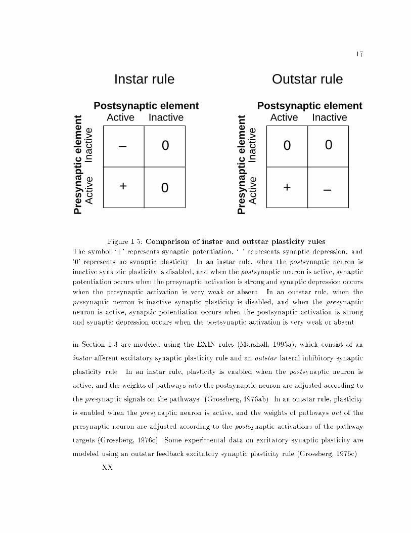
17Postsynaptic element

Pre

syn

apti

c el

emen

t Active Inactive

Act

ive

Inac

tive

Instar rule

Postsynaptic element

Pre

syn

apti

c el

emen

t Active Inactive

Act

ive

Inac

tive

Outstar rule

+ +

0 00

0Figure 1.5: Comparison of instar and outstar plasticity rules.The symbol `+' represents synaptic potentiation, `{' represents synaptic depression, and`0' represents no synaptic plasticity. In an instar rule, when the postsynaptic neuron isinactive synaptic plasticity is disabled, and when the postsynaptic neuron is active, synapticpotentiation occurs when the presynaptic activation is strong and synaptic depression occurswhen the presynaptic activation is very weak or absent. In an outstar rule, when thepresynaptic neuron is inactive synaptic plasticity is disabled, and when the presynapticneuron is active, synaptic potentiation occurs when the postsynaptic activation is strongand synaptic depression occurs when the postsynaptic activation is very weak or absent.in Section 1.3 are modeled using the EXIN rules (Marshall, 1995a), which consist of aninstar a�erent excitatory synaptic plasticity rule and an outstar lateral inhibitory synapticplasticity rule. In an instar rule, plasticity is enabled when the postsynaptic neuron isactive, and the weights of pathways into the postsynaptic neuron are adjusted according tothe presynaptic signals on the pathways. (Grossberg, 1976ab). In an outstar rule, plasticityis enabled when the presynaptic neuron is active, and the weights of pathways out of thepresynaptic neuron are adjusted according to the postsynaptic activations of the pathwaytargets (Grossberg, 1976c). Some experimental data on excitatory synaptic plasticity aremodeled using an outstar feedback excitatory synaptic plasticity rule (Grossberg, 1976c).XX

18The instar excitatory and the outstar excitatory synaptic plasticity rules are partof the adaptive resonance theory (ART) network (Carpenter & Grossberg, 1987). Theinstar excitatory and the outstar inhibitory synaptic plasticity rules form the EXIN model(Marshall, 1995a). Thus, the synaptic plasticity rules used in the models in this dissertationhave been previously used to model some cortical properties. However, the work presented inthis dissertation is original in applying these rules (especially the lateral inhibitory plasticityrule), to some classical problems { classical \rearing" conditioning, long-term potentiation,and long-term depression { and to some recently discovered phenomena { ocular dominancechanges during visual deprivation with cortical infusion of pharmacological agents inanimals in their critical period, dynamic receptive �eld changes in adult animals afterarti�cial scotoma conditioning, and changes in receptive �eld topography after intracorticalmicrostimulation and local peripheral stimulation in adult animals. Novel explanationsare proposed for receptive �eld changes in adults, long-term potentiation and long-termdepression, and ocular dominance plasticity during visual deprivation with cortical infusionof pharmacological agents. Furthermore, novel experiments are suggested based on themodeling.1.5 Relation to previous theoriesNeural networks that self-organize using unsupervised learning rules can modelhow cortical circuitry and receptive �eld properties form during biological developmentand how they change in adults in response to the input environment (Grossberg, 1982;von der Malsburg & Singer, 1988; Willshaw & von der Malsburg, 1976). Thus,self-organization provides a uni�ed framework for discussing and understanding synapticplasticity, cortical circuits, receptive �eld properties, and behavior.A unifying theory based on self-organization has succeeded in modeling severalcortical properties and functions { disparity selectivity (Marshall, 1990c), motion selectivityand grouping (Marshall, 1990a, 1995b; Schmitt & Marshall, 1995, 1996), visual inertia(Hubbard & Marshall, 1994), the aperture problem (Marshall, 1990a), length selectivityand end-stopping (Marshall, 1990b), visibility/invisibility and depth from occlusion

19events (Marshall & Alley, 1993; Marshall et al., 1996a), depth from motion parallax(Marshall, 1989), motion smearing (Martin & Marshall, 1993), orientation selectivity(Marshall, 1990d), and stereomatching (Marshall & Kalarickal, 1995; Marshall et al., 1996b).The proposed research provides further support for a uni�ed theory of cortical processingbased on self-organization.Recent neural network models (Marshall, 1995a; Marshall & Gupta, 1998)have demonstrated that the outstar lateral inhibitory synaptic plasticity rule leads tothe development of neurons with high stimulus feature selectivity and high stimulusdiscrimination. Lateral inhibitory synaptic plasticity also reduces redundancy in neuralcoding and produces sparse, distributed codes for input stimuli (Marshall & Gupta, 1998;Sirosh et al., 1996). Marshall (1995a) has shown that neural networks using the instara�erent excitatory synaptic plasticity rule in concert with the outstar inhibitory synapticplasticity rule can self-organize to represent multiple simultaneously presented input stimuli,represent transparency, perform scale and context sensitive processing, and maintain highdiscrimination in the presence of noise.XX1.6 Emphasis on lateral inhibitory interactionsIn this dissertation, the role of lateral inhibitory plasticity in producing corticalplasticity is emphasized. In the cortex, there are lateral excitatory and lateralinhibitory pathways (Gilbert & Wiesel, 1989; McGuire et al., 1991; Somogyi et al., 1983;Somogyi & Martin, 1985). The lateral excitatory and inhibitory pathways terminate onexcitatory and inhibitory neurons. Stimulation of thalamocortical pathways producesa monosynaptic excitatory postsynaptic potential (EPSP) and disynaptic inhibitorypostsynaptic potential (IPSP) in primary visual cortical neurons, and disynaptic EPSPsare occasionally produced (Gil & Amitai, 1996; Ferster, 1989). Direct stimulation of lateralexcitatory pathways have an excitatory e�ect at low stimulation strength and have aninhibitory e�ect at high stimulation strength (Gil & Amitai, 1996; Weliky et al., 1995).In addition, cortical neurons receive feedback excitatory inputs from other cortical layers.

20Thus, the response properties of cortical neurons depends on a combination of the variouspathways onto the neurons.The EXIN model, however, does not have lateral excitatory connections. But,lateral excitatory connections with signal transmission latencies have been used inconjunction with the EXIN rules to model several aspects of visual motion perception(Hubbard & Marshall, 1994; Marshall, 1989, 1990a, 1991, 1995b; Marshall & Alley, 1993;Martin & Marshall, 1993). Plasticity in lateral excitatory pathways has been used indevelopment of topologically ordered RFs (Sirosh & Miikkulainen, 1994b).In the EXIN simulations presented in the dissertation, lateral excitatory pathwayswere not incorporated. This simpli�ed the simulations. The use of lateral inhibitorypathways alone is justi�ed by the observation that in the cortex, suprathreshold stimulationproduces overall inhibitory lateral interaction (Ferster, 1989; Gil & Amitai, 1996;Toth et al., 1996; Weliky et al., 1995). The overall lateral interaction is facilitatory whenthe input stimulus is subthreshold (Toth et al., 1996). Combined measurement of spikingpoint-spread using extracellular recording and optical point-spread in cat primary visualcortex showed that the spiking point-spread accounts for only 5% of the optical point-spread; the remainder of the optical point-spread was largely caused by inhibition (Das &Gilbert, 1995a). Thus, the EXIN model can be viewed is a functional model that describesthe overall e�ect of lateral interactions in the cortex.Furthermore, lateral inhibition strongly in uences most cortical properties.Several stimulus feature speci�cities of cortical neurons such as orientation selectivity andspatial frequency selectivity are abolished by cortical infusion of a GABAA antagonist(Sillito, 1975, 1977, 1979). Blocking intracortical inhibition also reveals new peripheralregions capable of evoking neuronal responses (Lane et al., 1997; Sillito et al., 1981). Thus,changes in overall lateral inhibitory strength can contribute to cortical plasticity.Neurophysiologically, the EXIN lateral inhibitory synaptic plasticity rule could berealized in a disynaptic circuit containing a lateral excitatory horizontal connection (eithershort- or long-range) and an inhibitory interneuron, either by modifying the excitatoryweights from the excitatory neuron or by changing the inhibitory weight from the inhibitoryneuron (Darian-Smith & Gilbert, 1994, 1995; Das & Gilbert, 1995ab; Gilbert et al., 1996;

21Hirsch & Gilbert, 1993).XX1.7 Thesis statementLateral inhibitory plasticity is crucial in modeling a diverse set of cortical andbehavioral properties and functions. Together with excitatory plasticity, it allows theself-organization of neural network models that exhibit many fundamental propertiesfound in neurobiological experiments: the cortical, synaptic, and behavioral reorganizationthat follows classical rearing conditioning, arti�cial scotoma conditioning, retinal lesions,intracortical microstimulation, repetitive peripheral stimulation, and neuropharmacologicalmanipulations. These reorganization properties can be seen as manifestations of the moregeneral properties of high selectivity, high discrimination, and e�cient representation thatemerge from lateral inhibitory synaptic plasticity.1.8 Overall contributions and signi�canceExperimental data from di�erent conditioning paradigms { stimulation ofindividual pathways and isolated postsynaptic neurons, classical rearing, arti�cial scotomaconditioning, retinal lesions, local peripheral stimulation, intracortical microstimulation,and pharmacological treatments { are modeled using a small set of simple synaptic plasticityrules. This work1. models the phenomena of long-term potentiation and depression;2. models ocular dominance plasticity in during classical rearing procedures and duringvisual deprivation with pharmacological infusions in the cortex;3. provides a complete model for dynamic receptive �eld changes produced by arti�cialscotoma conditioning;4. models changes in receptive �eld properties after retinal lesions;5. models changes in receptive �eld topography after intracortical microstimulation;

226. models changes in receptive �eld properties and improvement in stimulusdiscrimination after repeated localized peripheral stimulation;7. compares the EXIN model with other models for synaptic and cortical plasticity;8. demonstrates the dramatic e�ects that are produced by the subtle distinctions betweeninstar, outstar, and covariance rules;9. analyzes the role of lateral inhibitory synaptic plasticity in neuronal feature selectivityand stimulus discrimination during development and adult cortical plasticity; and10. suggests novel and feasible experiments to test predictions of the models.Overall, the dissertation provides further support for a uni�ed theory ofcortical processing based on self-organization and highlights the possible role of lateralinhibitory synaptic plasticity in cortical development and adult cortical plasticity. Novelexperiments and the predictions of the models are provided to facilitate further experimentalinvestigations of cortical development and adult cortical plasticity. Furthermore, thesimulations demonstrate that the outstar lateral inhibitory synaptic plasticity rule issu�cient to model the receptive �eld changes produced by arti�cial scotoma conditioningand localized peripheral stimulation in adult animals. Because arti�cial scotomaconditioning and localized peripheral stimulation are similar to the conditioning proceduresused in perceptual learning, lateral inhibitory synaptic plasticity may also be involved inperceptual learning.1.9 Outline of the dissertationThe dissertation is organized as follows. The main chapters (Chapters 2{6) areeach self-contained and can be read independently of one another. In these chapters, speci�ccortical plasticity phenomena are modeled, and novel experiments are proposed based onthe predictions of the models.In Chapter 2, the phenomena of long-term potentiation (LTP) and long-termdepression (LTD) are modeled using the instar and the outstar excitatory synaptic plasticity

23rules. The experiments on synaptic plasticity provide direct evidence for the relationshipbetween correlation in pre- and postsynaptic activation and synaptic plasticity. The workinghypothesis is that long-term synaptic plasticity is responsible for the development andre�nement of cortical properties and functions during early postnatal stages and for corticalplasticity in adults. Thus, the rules for synaptic plasticity used for modeling corticaldevelopment and adult cortical plasticity must be consistent with data on long-term synapticplasticity. This chapter shows that the instar and the outstar excitatory synaptic plasticityrules model data on LTP and LTD more accurately than a popular excitatory synapticplasticity rule, the BCM rule (Bienenstock, Cooper, & Munro, 1982). Furthermore, theproperties of the outstar lateral inhibitory synaptic plasticity rule are characterized andcompared with the few available experimental data on inhibitory synaptic plasticity. Thefunctional roles of the instar and outstar excitatory and the outstar lateral inhibitorysynaptic plasticity rules in development of cortical properties are discussed.Chapter 3 presents computer simulations of the e�ects of a�erent excitatoryand lateral inhibitory synaptic plasticity rules on ocular dominance, responsiveness, andreceptive �eld width of model cortical neurons during classical rearing conditioning. Themodel is based on the EXIN synaptic plasticity rules (Marshall, 1995a), which consist of theinstar a�erent excitatory and the outstar lateral inhibitory synaptic plasticity rules. In themodel, the a�erent excitatory synaptic plasticity plays the primary role in ocular dominanceplasticity during the classical rearing paradigms, and lateral inhibitory interactions producesecondary ocular dominance changes. The relationship between the strength of lateralinhibitory pathway weights and the ocular dominance distribution after normal rearing isdemonstrated.In Chapter 4, the e�ects of cortical infusion of an NMDA antagonist(Bear et al., 1990) and a GABA agonist (Reiter & Stryker, 1988) during monoculardeprivation and e�ects of cortical infusion of an NMDA antagonist on ocular dominance inadult animals (Kasamatsu et al., 1997, 1998a) are modeled. The salient e�ects producedby the model are caused by lateral inhibitory interactions, and the model is consistentwith experimental data on excitatory synaptic plasticity in the presence of NMDA receptorantagonists and postsynaptic hyperpolarization.

24In Chapter 5, the dynamic changes in the size, shape, and position of neuronalreceptive �elds in response to arti�cial scotoma conditioning (Pettet & Gilbert, 1992;DeAngelis et al., 1995) and retinal lesions (Darian-Smith & Gilbert, 1995) are modeled usingthe EXIN synaptic plasticity rules. The e�ects produced by the EXIN rules are comparedwith those produced by models based on neuronal adaptation (Xing & Gerstein, 1994)and on the LISSOM learning rules (Sirosh et al., 1996). The comparison of the e�ectsproduced by the models and the neurophysiological data show that the outstar lateralinhibitory synaptic rule and the LISSOM lateral excitatory rule provide the best �t forthe experimental data. A novel complementary scotoma conditioning experiment, in whichstimulation of scotoma and non-scotoma regions are alternated repeatedly, is proposed todi�erentiate the outstar lateral inhibitory synaptic rule and the LISSOM lateral excitatorysynaptic plasticity rule.A model for the dynamic changes in the size and position of neuronal receptive�elds in response to intracortical microstimulation (Recanzone et al., 1992b) based on theEXIN synaptic plasticity rules is presented in Chapter 6. Changes in cortical topography,receptive �eld properties, and stimulus discrimination following local repetitive peripheralstimulation (Jenkins et al., 1990; Recanzone et al., 1992acde) are also modeled. Thee�ects of the outstar lateral inhibitory synaptic plasticity rule during ICMS and peripheralstimulation on the relationship between receptive �eld size and cortical magni�cation is alsoanalyzed.The �nal chapter, Chapter 7, summarizes the main results of the dissertation andpresents several research questions related to the issues addressed in this dissertation.

Chapter 2Comparison of generalizedHebbian rules for long-termsynaptic plasticityAbstractA large variety of synaptic plasticity rules have been used in models of excitatorysynaptic plasticity (Brown et al., 1990). These rules are generalizations of the Hebbianrule and have some properties consistent with experimental data on long-term excitatorysynaptic plasticity, but they also have some properties inconsistent with experimentaldata. For example, the BCM rule (Bear et al., 1987; Bienenstock et al., 1982) produceshomosynaptic potentiation and depression, which has been observed experimentally(Artola et al., 1990; Dudek & Bear, 1992; Kirkwood et al., 1993; Fr�egnac et al., 1994;Yang & Faber, 1991). But the BCM rule is also inconsistent with some experimentalresults; e.g., the BCM rule cannot produce heterosynaptic depression (Abraham &Goddard, 1983; Lynch et al., 1977). In addition, long-term synaptic plasticity in inhibitorypathways has been emphasized in some models of cortical function (Marshall, 1990abc,1995a; Sirosh et al., 1996), but experimental data on inhibitory synaptic plasticity is

26sparse. This paper compares three popular excitatory synaptic plasticity rules { the BCMrule, the instar rule (Grossberg, 1972, 1976ab; Kohonen, 1988; Levy & Burger, 1987;Levy & Desmond, 1985; Marshall, 1995a), and the outstar excitatory rule (Grossberg, 1976c;Rescorla & Wagner, 1972) { and presents and characterizes the outstar inhibitory synapticplasticity rule (Marshall, 1995a). These rules are evaluated by comparing their predictionswith neurobiological data.2.1 IntroductionThere is a large number of synaptic plasticity rules that have been proposed tomodel developmental, structural, functional, cognitive, and behavioral properties of animalbrains (Bienenstock et al., 1982; Grossberg, 1972, 1976abc, 1980, 1982; Kohonen, 1987,1988; Linsker, 1986abc, 1988; von der Malsburg, 1973; Marshall, 1995a; Miller et al, 1989;Rescorla & Wagner, 1972; Rumelhart & McClelland, 1986; Sejnowski, 1977ab; Sirosh &Miikkulainen, 1994b). Experimentally, synaptic plasticity in excitatory synapses hasbeen extensively studied in hippocampus (Brown et al., 1990), sensory neocortex(Kirkwood et al., 1993), and cerebellum (Crepel et al., 1995). But there have beenvery few studies comparing abstract synaptic plasticity rules with experimental data(e.g., Bear et al., 1987; Dudek & Bear, 1992). In addition, only a few models useand emphasize the role of inhibitory synaptic plasticity (e.g., Marshall, 1990abc, 1995a;Marshall & Gupta, 1998; Sirosh & Miikkulainen, 1996) in development of importantcomputational and neurobiological properties.In this paper, a widely studied (both theoretically and experimentally)synaptic plasticity rule { the BCM rule (Bear et al., 1987; Bienenstock et al., 1982;Clothiaux et al., 1991) { is compared with two generalized Hebbian (Brown et al., 1990)excitatory synaptic plasticity rules { an instar excitatory synaptic plasticity rule(Grossberg, 1972, 1976ab; Kohonen, 1988; Levy & Desmond, 1985; Levy & Burger, 1987;Marshall, 1995a) and an outstar excitatory synaptic plasticity rule (Grossberg, 1976c;Rescorla & Wagner, 1972) { and with the experimental data on excitatory synapticplasticity. The plasticity governed by an instar rule is enabled when the postsynaptic

27neuron is activated, and excitatory pathways into the neuron undergo synaptic plasticity(Grossberg, 1972, 1976ab). In contrast, the plasticity governed by an outstar rule is enabledwhen the presynaptic neuron or presynaptic element is activated, and excitatory pathwaysout of the neuron undergo synaptic plasticity (Grossberg, 1976c). This paper furthermoredescribes an outstar inhibitory synaptic plasticity rule and elucidates and compares therule's properties with the currently sparse experimental database on inhibitory synapticplasticity.Many experimental results on excitatory synaptic plasticity have been attributedto the covariance rule (Sejnowski, 1977ab; Stanton & Sejnowski, 1990) or the BCM rule(Bear et al., 1987; Dudek & Bear, 1992). This paper shows that many of the experimentaldata are also consistent with the instar and outstar excitatory synaptic plasticity rules. Onlya few experiments are available today to illuminate the subtleties of the di�erent rules. Thus,novel experiments are proposed, and explicit predictions of the synaptic plasticity rules aremade. The plausible functional capabilities of the rules are also discussed.The instar excitatory synaptic plasticity rule alone can be used to self-organize aneural network that categorizes arbitrary input patterns (Carpenter & Grossberg, 1987;Grossberg, 1976ab, 1980, 1982; Marshall, 1995a; Nigrin, 1993). The instar excitatorysynaptic plasticity rule moves the synaptic input weight vector of an active neuron closerto the presynaptic activation vector.The outstar excitatory synaptic plasticity rule has been used to governsynaptic e�cacy of feedback pathways roles (Baloch & Grossberg, 1997; Carpenter &Grossberg, 1987; Grunewald & Grossberg, 1997; Grossberg et al., 1997a; Schmitt &Marshall, 1995; Nigrin, 1993) and to make predictions in classical conditioning protocols(Pavlov, 1927; Rescorla & Wagner, 1972; Schmajuk, 1997). The outstar excitatory synapticplasticity rule moves the synaptic output weight vector of an active neuron closer to thepostsynaptic activation vector.The outstar lateral inhibitory synaptic plasticity rule produces strong lateralinhibitory pathways between neurons that are consistently coactivated (Marshall, 1995a).Neurons are consistently coactivated if they are selective for similar patterns, and the stronglateral inhibition between such neurons improves stimulus discriminability. According

28to the outstar lateral inhibitory synaptic plasticity rule, lateral inhibitory pathwaysbetween neurons that are not consistently coactivated become weak. Neurons are notconsistently coactivated if they are selective for very di�erent input patterns. This selectivedevelopment of lateral inhibitory pathways between neurons leads to exclusive allocationand simultaneous representation of separate multiple patterns, e.g., transparently overlaidsurfaces (Marshall, 1995a; Marshall et al., 1996b).The instar excitatory and the outstar inhibitory synaptic plasticity rules have beenused together within a single model, and they are together referred to as the EXIN synapticplasticity rules (Marshall, 1995a). The EXIN rules develop an e�cient representation ofinput patterns according to their distribution in an input environment. The EXIN rulesself-organize networks capable of representing multiple superimposed patterns, ambiguouspatterns, overlapping patterns at di�erent scales, and contextually constrained patternsstarting from completely nonspeci�c a�erent excitatory and lateral inhibitory pathwayweights (Marshall, 1995a). In EXIN networks, the instar excitatory synaptic plasticityrule modi�es weights so that the active neurons become more responsive to the currentlypresented input pattern. The development of weights of lateral inhibitory pathwaysaccording to the outstar lateral inhibitory synaptic plasticity rule ensures that di�erentneurons become selective to di�erent input patterns. Yet if the input environment containsseveral similar patterns, the outstar lateral inhibitory synaptic plasticity rule developsstrong lateral inhibitory pathways between neurons selective for the similar input patterns,thereby producing high discrimination. In EXIN networks, lateral inhibitory pathways fromoften activated neurons to unresponsive neurons weaken, thereby making the unresponsiveneurons more likely to respond to some input. This feature of the EXIN lateral inhibitorysynaptic plasticity rule is comparable to that of \conscience" rules (DeSieno, 1988).EXIN synaptic plasticity rules have been used to model the development ofvisual motion selectivity and grouping (Marshall, 1990a), visual inertia (Hubbard &Marshall, 1994), motion integration in the aperture problem (Marshall, 1990a), lengthselectivity and end-stopping (Marshall, 1990b), depth perception from occlusion events(Marshall & Alley, 1993; Marshall et al., 1996a), depth from motion parallax(Marshall, 1989), motion smearing (Martin & Marshall, 1993), orientation selectivity

29(Marshall, 1990d), stereomatching (Marshall et al., 1996b), dynamic receptive �eld changesproduced by arti�cial scotoma conditioning (Kalarickal & Marshall, 1997b; Marshall &Kalarickal, 1997), and changes in somatosensory cortical RF structure after intracorticalmicrostimulation (Kalarickal & Marshall, 1998b).The BCM synaptic plasticity rule (Bienenstock et al., 1982) has been used to modelthe results of \classical" rearing conditions (Bienenstock et al., 1982; Clothiaux et al., 1991).The important feature of the BCM rule is its adaptable synaptic modi�cation threshold. Theadaptable synaptic modi�cation threshold is nonlinearly related to the activation historyof the postsynaptic neuron and contributes to the development of selectivity and stabilityof the system in the absence of lateral inhibition (Bienenstock et al., 1982; Intrator &Cooper, 1992; Shouval et al., 1996). The synaptic modi�cation function proposed by theBCM rule has been shown to be in partial agreement with studies on synaptic plasticity(Bear et al., 1987; Dudek & Bear, 1992; Kirkwood et al., 1993). These properties cannot beproduced by some other synaptic plasticity rules, such as the covariance rule (Sejnowski &Stanton, 1990; Brown & Chattarji, 1995).In the cortex, interactions via lateral pathways may in uence cortical neuronalproperties (Gilbert et al., 1990). In fact, geniculocortical synapses comprise only 4% to 24%of all synapses received by layer 4 neurons (Ahmed et al., 1994; Einstein et al., 1987; Peters &Payne, 1993). Recent models (e.g., Kalarickal & Marshall, 1997b, 1998b; Marshall, 1989,1990abc; Marshall & Alley, 1993; Marshall et al., 1996ab; Marshall & Kalarickal, 1997;Martin & Marshall, 1993; Sirosh et al., 1996; Somers et al., 1995) have emphasizedlateral intracortical interactions to model several cortical and perceptual properties. Inthe simulations the synaptic plasticity rules are applied in a small, simple model neuralnetwork to demonstrate the properties that can be produced by the rules because of networkinteractions.2.2 MethodsIn the simulations, a simple two layered network was used. Layer 1 may correspondto part of the lateral geniculate nucleus (LGN), and Layer 2 may correspond to part of the

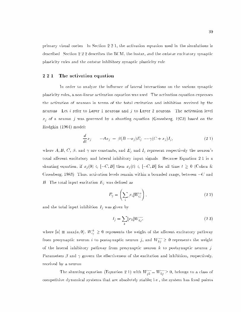
30primary visual cortex. In Section 2.2.1, the activation equation used in the simulations isdescribed. Section 2.2.2 describes the BCM, the instar, and the outstar excitatory synapticplasticity rules and the outstar inhibitory synaptic plasticity rule.2.2.1 The activation equationIn order to analyze the in uence of lateral interactions on the various synapticplasticity rules, a non-linear activation equation was used. The activation equation expressesthe activation of neurons in terms of the total excitation and inhibition received by theneurons. Let i refer to Layer 1 neurons and j to Layer 2 neurons. The activation levelxj of a neuron j was governed by a shunting equation (Grossberg, 1972) based on theHodgkin (1964) model:ddtxj = �Axj + �(B � xj)Ej � (C + xj)Ij ; (2.1)where A;B, C, �, and are constants, and Ej and Ij represent respectively the neuron'stotal a�erent excitatory and lateral inhibitory input signals. Because Equation 2.1 is ashunting equation, if xj(0) 2 [�C;B] then xj(t) 2 [�C;B] for all time t � 0 (Cohen &Grossberg, 1983). Thus, activation levels remain within a bounded range, between �C andB. The total input excitation Ej was de�ned asEj = Xi [xi]W+ij! ; (2.2)and the total input inhibition Ij was given byIj =Xk [xk]W�kj ; (2.3)where [a] � max(a; 0), W+ij � 0 represents the weight of the a�erent excitatory pathwayfrom presynaptic neuron i to postsynaptic neuron j, and W�kj � 0 represents the weightof the lateral inhibitory pathway from presynaptic neuron k to postsynaptic neuron j.Parameters � and govern the e�ectiveness of the excitation and inhibition, respectively,received by a neuron.The shunting equation (Equation 2.1) with W�jk = W�kj � 0, belongs to a class ofcompetitive dynamical systems that are absolutely stable; i.e., the system has �xed points

31(stable equilibrium states) for any choice of parameters (Cohen & Grossberg, 1983). Theneuronal activations in such a system are guaranteed to reach stable equilibrium values forall synaptic weight values, with the restriction that W�jk = W�kj � 0 for all pairs of neurons.However, it is not known whether the shunting equation remains absolutely stablewhen W�jk 6= W�kj for some pairs of neurons. Nevertheless, empirically the shunting equationreaches an equilibrium state even when reciprocal pairs of lateral inhibitory weights are notequal.2.2.2 Synaptic plasticity rulesThis section brie y describes the BCM rule, the instar excitatory synapticplasticity rule, the outstar excitatory synaptic plasticity rule, and the outstar inhibitorysynaptic plasticity rule.The BCM excitatory synaptic plasticity ruleAccording to the theory presented by Bienenstock, Cooper, & Munro (1982),synaptic weights change over time as a function of local and global variables.Bienenstock et al. (1982) proposed a synaptic plasticity rule, now known as the BCM rule, tomodel ocular dominance plasticity in animals during a critical period. The focus of the BCMsynaptic plasticity rule is a variable threshold, which depends on the postsynaptic activationhistory, and which controls whether the synaptic weights undergo potentiation or depression(Bienenstock et al., 1982; Clothiaux et al., 1991; Intrator & Cooper, 1992). According to arecent formulation of the BCM synaptic plasticity rule (Clothiaux et al., 1991; Intrator &Cooper, 1992; Shouval et al., 1996),ddtW+ij (t) = � � (xj (t) ; �j (t)) xi (t) ; (2.4)where xi is the presynaptic activation, xj is the postsynaptic activation, and � is a smallpositive constant that determines the magnitude of the synaptic modi�cation. The function� is � (xj (t) ; �j(t)) = xj(t) (xj(t) � �j(t)) (2.5)

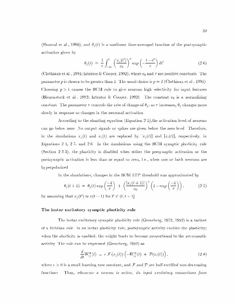
32(Shouval et al., 1996), and �j(t) is a nonlinear time-averaged function of the postsynapticactivation given by �j(t) = 1� Z t�1 �xj(t0)c0 �p exp�� t � t0� �dt0 (2.6)(Clothiaux et al., 1991; Intrator & Cooper, 1992), where c0 and � are positive constants. Theparameter p is chosen to be greater than 1. The usual choice is p = 2 (Clothiaux et al., 1991).Choosing p > 1 causes the BCM rule to give neurons high selectivity for input features(Bienenstock et al., 1982; Intrator & Cooper, 1992). The constant c0 is a normalizingconstant. The parameter � controls the rate of change of �j ; as � increases, �j changes moreslowly in response to changes in the neuronal activation.According to the shunting equation (Equation 2.1),the activation level of neuronscan go below zero. No output signals or spikes are given below the zero level. Therefore,in the simulations xj(t) and xi(t) are replaced by [xj(t)] and [xi(t)], respectively, inEquations 2.4, 2.5, and 2.6. In the simulations using the BCM synaptic plasticity rule(Section 2.3.3), the plasticity is disabled when either the presynaptic activation or thepostsynaptic activation is less than or equal to zero, i.e., when one or both neurons arehyperpolarized.In the simulations, changes in the BCM LTP threshold was approximated by�j(t+ 1) = �j(t) exp��1� � + � [xj(t+ 1)]c0 �p �1� exp��1� �� ; (2.7)by assuming that xj(t0) � x(t + 1) for t0 2 (t; t+ 1].The instar excitatory synaptic plasticity ruleThe instar excitatory synaptic plasticity rule (Grossberg, 1972, 1982) is a variantof a Hebbian rule. In an instar plasticity rule, postsynaptic activity enables the plasticity;when the plasticity is enabled, the weight tends to become proportional to the presynapticactivity. The rule can be expressed (Grossberg, 1982) asddtW+ij (t) = � F (xj(t))��W+ij (t) + P(xi(t))� ; (2.8)where � > 0 is a small learning rate constant, and F and P are half-recti�ed non-decreasingfunctions. Thus, whenever a neuron is active, its input excitatory connections from

33active neurons tend to become slightly stronger, while its input excitatory connectionsfrom inactive neurons tend to become slightly weaker. Neuron activations remain within[�C;B] according to the shunting equation (Section 2.2.1); this causes the excitatory weightvalues to be bounded, because according to Equation 2.8, W+ij (t) 2 [0;P(B)] for t � 0, ifW+ij (0) 2 [0;P(B)] and xi(t) � B (Grossberg, 1982).The outstar excitatory synaptic plasticity ruleIn an outstar plasticity rule (Grossberg, 1972, 1982), presynaptic activity enablesthe plasticity at a synapse; when the plasticity is enabled, the weight tends to becomeproportional to the postsynaptic activity. The rule can be expressed (Grossberg, 1982) asddtW+ij (t) = � G(xi(t)) ��W+ij (t) + Q(xj(t))� ; (2.9)where � > 0 is a small learning rate constant, and G and Q are half-recti�ed non-decreasingfunctions. The positions of xi and xj are reversed, compared with the instar rule. Thus,whenever a neuron is active, its output excitatory connections to active neurons tend tobecome slightly stronger, while its output excitatory connections to inactive neurons tend tobecome slightly weaker. Neuron activations remain within [�C;B] according to the shuntingequation (Section 2.2.1); this in turn causes the excitatory weight values to be boundedbetween 0 and Q(B) (Grossberg, 1982).The outstar lateral inhibitory synaptic plasticity ruleThe lateral inhibitory weights, W�jk, are modi�ed according to theanti-Hebbian rule ddtW�jk = � H(xj) ��W�jk + R(xk)� (2.10)(Marshall, 1995a; Marshall & Gupta, 1998) where � > 0 is a small learning rate constant,and H and R are half-recti�ed non-decreasing functions.Thus, whenever a neuron is active, its output inhibitory connections to other activeneurons tend to become slightly stronger (i.e., more inhibitory), while its output inhibitoryconnections to inactive neurons tend to become slightly weaker . Neuron activations remain

34within [�C;B] according to the shunting equation (Equation 2.1); this causes the inhibitoryweight values to remain bounded as well, between 0 and R(B) (Grossberg, 1982).2.3 ResultsIn order to evaluate the BCM rule, the instar and outstar excitatory synapticplasticity rules, and the outstar lateral inhibitory synaptic plasticity rule in comparisonto experimental data, the properties of the rules are studied by analysis and computersimulations.In Section 2.3.1, synaptic plasticity in pathways to a postsynaptic neuron isexpressed analytically as a function of input excitation according to the BCM, the instar,and the outstar excitatory synaptic plasticity rules, by making simplifying assumptionsabout the postsynaptic activation. Lateral inhibitory synaptic plasticity, according to theoutstar lateral inhibitory synaptic plasticity rule, is expressed analytically as a function ofinput excitation in Section 2.3.2.In Section 2.3.3, the subtle properties of the BCM, the instar, and the outstarexcitatory synaptic plasticity rules are studied as a function of pre- and postsynapticactivation, initial synaptic weight, and simultaneous stimulation of di�erent pathways. Thee�ects of lateral inhibitory interactions are also explored.In some experiments (Artola et al., 1990; Fr�egnac et al., 1994;Kirkwood et al., 1993), the conditioning stimulation was appliedat the white matter{layer 6 border. Stimulation at the white matter{layer 6 border canactivate geniculocortical and corticocortical feedback pathways (Kirkwood et al., 1993).Many models (e.g., Carpenter & Grossberg, 1987; Grossberg, 1980; Grossberg et al., 1997a;Grossberg & Merrill, 1997; Grunewald & Grossberg, 1997; Nigrin, 1993) use both the instarand the outstar excitatory synaptic plasticity rules. In these models, the instar rule governssynaptic plasticity in a�erent excitatory pathways, and the outstar rule governs synapticplasticity in feedback excitatory pathways. Thus, the e�ects of a combination of the instarand the outstar excitatory synaptic plasticity rules are studied in Section 2.3.4.Finally, Section 2.3.5 presents the properties of the outstar lateral inhibitory

35synaptic plasticity rule as a function of the input excitation to model neurons,pre- and postsynaptic activation, and initial inhibitory synaptic weight.Computer simulations were used to study synaptic plasticity in Sections 2.3.3{2.3.5because, with lateral interactions, the activation equation does not have a closed-formformula in the model neural network.2.3.1 Analyses of excitatory synaptic plasticity rulesIn this section, the postsynaptic activation of a neuron is �rst expressed as afunction of presynaptic stimulation by supposing that the neuron does not receive anyinhibitory input and that postsynaptic activation is linearly related to input excitation.These simplifying assumptions are helpful in deriving analytical expressions that elucidatethe important properties of the synaptic plasticity rules.Let x > 0 represent the strength of presynaptic stimulation applied to excitatorypathways to postsynaptic neuron j. Let xj represent the activation level of the postsynapticneuron j. Let W+ij be the weight of the excitatory synapse from the a�erent i and toneuron j. The presynaptic activation of unstimulated pathways to neuron j is zero.Neuronal activation as a function of input stimulation.The excitation received by neuron j isEj = Xi 2 active presynaptic input[xi]W+ij ; (2.11)where [xi] is de�ned to mean max(0; xi). For each stimulated excitatory pathway i toneuron j, the presynaptic activation xi = x in this test simulation. ThusEj = E x (2.12)where E =Pi 2 active presynaptic inputW+ij . From Equation 2.1, the activation level ofneuron j, at equilibrium, isxj = �BEj � CIjA+ �Ej + Ij = �BE x� CIjA + �E x+ Ij (2.13)

36In general, the relationship between xj and x is di�cult to determine because oflateral inhibition. It is possible that with increasing x, xj decreases because of increasing Ij(Figure 2.12). If j is the only active neuron in a winner-take-all (WTA) network, xj canincrease with increasing x (Figure 2.8). However, the activation of a neuron can increasemonotonically with presynaptic activation even if there are other active neurons sendinginhibition to it (Figure 2.13).To facilitate analytical expressions for synaptic plasticity, the following simplifyingassumptions are made: (1) the Layer 2 neuronal responses are linearly related to the inputexcitation, i.e. xj / Ej , and (2) the network behaves in a WTA fashion (the winner neurondoes not receive any lateral inhibition).Assuming that the activation of layer 2 neurons is in their linear region,xj = �Ej = �Ex. Under the WTA assumption, the winner neuron j does not receiveany inhibition; i.e., Ij = 0, and therefore, the equilibrium activation of neuron j, isxj = �BEjA+ �Ej = �BE xA+ �E x: (2.14)In this case, the activation of the winner neuron monotonically increases with inputexcitation.Analysis of the BCM excitatory synaptic plasticity ruleAssuming that the activation of neuron j is in its linear region, letxj = �Ej = �Ex. Substituting for xj in Equation 2.4, and because x > 0, the BCMexcitatory synaptic plasticity rule becomesddtW+ij = ��Ex (�Ex� �j)x: (2.15)The synaptic weight change as a function of the presynaptic stimulation strength x,controlled by Equation 2.15, is shown in Figure 2.1.Under a WTA assumption, the equilibrium activation level of the winner neuron,j, is given by Equation 2.14. Substituting the value of xj in the BCM rule (Equation 2.4),and because x > 0, Equation 2.4 becomesddtW+ij = � �BE xA+ �E x � �BE xA+ �E x � �j�x: (2.16)

37

0.0 0.2 0.4 0.6 0.8 1.0-0.10

-0.05

0.00

0.05

0.10

0.15

0.20

Postsynaptic activation

Syn

aptic

pla

stic

ity (

x 0.

1)WTA

0.0 0.2 0.4 0.6 0.8 1.0-0.10

-0.05

0.00

0.05

0.10

0.15

0.20

Postsynaptic activation

Syn

aptic

pla

stic

ity (

x 0.

1)

Linear

Figure 2.1: The BCM excitatory synaptic plasticity rule.The change in synaptic weight as a function of the presynaptic activity proposed by theBCM excitatory synaptic plasticity rule. The rule induces LTP when the postsynapticactivation level is above the LTP threshold (indicated by arrow-head) and induces LTDwhen the postsynaptic activation level is below the LTP threshold. In both curves, � = 0:05,E = 0:5, �j = 0:7, andWij = 0:5. In the WTA case, the synaptic plasticity curve is governedby Equation 2.14 with � = 1:0, A = 0:1, and B = 1:0. In the linear case, synaptic plasticityis governed by Equation 2.15 with � = 1:5.

38

-30

-20

-10

0

+10

+20

+30

Cha

nge

in E

PS

P s

lope

(%

)

Frequency of conditioning stimulation (Hz)1 10 100Figure 2.2: The BCM excitatory synaptic plasticity rule.The change in synaptic weight as a function of the presynaptic stimulation strength observedexperimentally by Dudek & Bear (1992). The presynaptic stimulation strength was variedby changing the frequency of conditioning stimulation, and synaptic weight was estimatedby measuring the slope of excitatory postsynaptic potential evoked by a test stimulation ofthe pathway. LTP is observed at higher presynaptic stimulation frequencies, and LTD isobserved at lower frequencies. Redrawn with permission, from Dudek and Bear (1992).

39The synaptic weight change as a function of presynaptic stimulation strength x > 0,according to Equation 2.16 is plotted in Figure 2.1.The graphs in Figure 2.1 are similar to the experimental data on synaptic weightmodi�cation as a function of presynaptic stimulation strength shown in Figure 2.2.In the general case, where inhibition is present, the weight change is obtained bysubstituting xj given by Equation 2.13 in Equation 2.4. Assuming that synaptic plasticityis blocked when the postsynaptic neuron is hyperpolarized and that x > 0,ddtW+ij = � " �BE x� CIjA + �E x+ Ij # " �BE x� CIjA+ �E x+ Ij #� �j! x: (2.17)The term �h�BE x� CIjA+�E x+ Ij i� �j� in Equation 2.17 captures the property of change in signof synaptic modi�cation. The multiplicative term � h�BE x� CIjA+�E x+ Ij ix modulates the rate ofchange. In the BCM synaptic plasticity rule, the weight change is zero when thepostsynaptic or the presynaptic activity is zero. The LTP threshold �j determines thesign of weight change in all stimulated pathways to an active postsynaptic neuron. Theshape of the function � is shown in Figure 2.3 for two di�erent values of the threshold �j(t).The two important features of the function � are that it changes sign at the modi�cationthreshold �j(t) and that it is zero when xj(t) is zero.The BCM synaptic plasticity rule exhibits homosynaptic depression when thepostsynaptic activation is less than the LTP threshold and homosynaptic potentiation whenthe postsynaptic activation is greater than the LTP threshold. Heterosynaptic depressionof the synaptic weight of inactive pathways to active neurons does not occur, because theBCM rule disables synaptic plasticity in unstimulated pathways.Analysis of the instar excitatory synaptic plasticity ruleAssuming that the activation of neuron j is in its linear region, letxj = �Ej = �Ex. Substituting for xj in Equation 2.8 with F(x) = [x], P(x) = [x], andx > 0, the instar excitatory synaptic plasticity rule becomesddtW+ij = ��Ex ��W+ij + x� : (2.18)

40

0.0 0.2 0.4 0.6 0.8 1.0-1.50

0.00

1.50

3.00

4.50

6.00

θ=0.5

θ=0.7

Postsynaptic activation

Syn

aptic

pla

stic

ity (

x 0.

1)

Low LTP threshold

0.0 0.2 0.4 0.6 0.8 1.0-1.50

0.00

1.50

3.00

4.50

6.00

θ=0.5

θ=0.7

Postsynaptic activation

Syn

aptic

pla

stic

ity (

x 0.

1)

High LTP threshold

Figure 2.3: Change in synaptic weight as a function of the postsynaptic activityusing the BCM rule.The BCM rule induces LTP (positive synaptic weight change) when the postsynapticactivation is above the variable synaptic modi�cation threshold � and induces LTD (negativesynaptic weight change) when it is below �.

41

0.0 0.2 0.4 0.6 0.8 1.0-0.10

-0.05

0.00

0.05

0.10

0.15

0.20

Presynaptic activation

Syn

aptic

pla

stic

ity (

x 0.

1)WTA

0.0 0.2 0.4 0.6 0.8 1.0-0.10

-0.05

0.00

0.05

0.10

0.15

0.20

Presynaptic activation

Syn

aptic

pla

stic

ity (

x 0.

1)

Linear

Figure 2.4: Change in synaptic weight as a function of the presynaptic activityusing the instar excitatory synaptic plasticity rule.The rule induces LTP when the presynaptic activation level is above the current synapticweight (which acts like the LTP threshold) and induces LTD when it is below the weight.In the WTA case, the synaptic plasticity curve is governed by Equation 2.17 with � = 0:05,� = 1:0, E = 0:5, A = 0:1, B = 1:0, and W+ij = 0:5. In the linear case, synaptic plasticityis governed by Equation 2.18 with � = 0:05, � = 1:5, E = 0:5, and W+ij = 0:5.

42The synaptic weight change as a function of presynaptic stimulation strength x, controlledby Equation 2.18, is shown inUnder a WTA assumption, the equilibrium activation level of the winner neuron jis given by Equation 2.14. Substituting the value of xj in the instar excitatory synapticplasticity rule (Equation 2.8), and assuming F(x) = [x], P(x) = [x], and x > 0, Equation 2.8becomes ddtW+ij = � �BE xA+ �E x ��W+ij + x� : (2.19)The synaptic weight change as a function of presynaptic stimulation strength x, accordingto Equation 2.19, is plotted in Figure 2.4. Figure 2.4. The graphs in Figure 2.4 are similarto the experimental data in Figure 2.2.In the general case, when inhibition is present, the weight change is obtained bysubstituting xj from Equation 2.13 in Equation 2.8 and assuming that F(x) = [x] andP(x) = [x]. When x > 0,ddtW+ij = � " �BE x� CIjA+ �E x+ Ij # ��W+ij + x� : (2.20)The term (�W+ij + x) in Equation 2.20 captures the property of change in sign of synapticmodi�cation. The multiplicative term � h�BE x� CIjA+�E x+ Ij i modulates the rate of change.In the instar excitatory synaptic plasticity rule, the weight change is zero whenthe postsynaptic activity less than or equal to zero. When a postsynaptic neuron is active,all unstimulated pathways to the active neuron weaken: P(xi) = 0 in Equation 2.8, andthus the right-hand side of Equation 2.8 is negative.The weight W+ij in Equation 2.8 behaves like a variable synaptic weightmodi�cation threshold, because W+ij is variable. In addition, W+ij is independent for everysynaptic connection.The instar excitatory synaptic plasticity rule exhibits homosynaptic depressionwhen the function P of presynaptic activation is less than the synaptic weight, and itexhibits homosynaptic potentiation when the the function P of presynaptic activation isgreater than the synaptic weight. Heterosynaptic depression of the synaptic weight ofinactive pathways occurs during postsynaptic activation.

43Analysis of outstar excitatory synaptic plasticity ruleAssuming that the activation of neuron j is in its linear region, letxj = �Ej = �Ex. Substituting for xj in Equation 2.9 with G(x) = [x], Q(x) = [x], andx > 0, the outstar excitatory synaptic plasticity rule becomesddtW+ij = �x ��W+ij + �Ex� : (2.21)The synaptic weight change as a function of presynaptic stimulation strength x, controlledby Equation 2.21, is shown in Figure 2.5.Under a WTA assumption, the equilibrium activation level of the winner neuron j,is given by Equation 2.14. Substituting the value of xj in the outstar excitatory synapticplasticity rule (Equation 2.9) with G(x) = [x], Q(x) = [x], and x > 0, Equation 2.9 becomesddtW+ij = �x��W+ij + �BE xA+ �E x� : (2.22)The synaptic weight change as a function of presynaptic stimulation strength x, accordingto Equation 2.22, is plotted in Figure 2.5. The graphs in Figure 2.5 are similar to theexperimental data on synaptic weight modi�cation as a function of presynaptic stimulationstrength shown in Figure 2.2.In the general case, the weight change is obtained by substituting xj fromEquation 2.13 in Equation 2.9 and assuming G(x) = [x] and Q(x) = [x]. Since x > 0,ddtW+ij = �x �W+ij + " �BE x� CIjA+ �E x+ Ij #! : (2.23)The term (�W+ij + h�BE x� CIjA+�E x+ Ij i) in Equation 2.23 captures the property of change in signof synaptic modi�cation, and the multiplicative term �x modulates the rate of change.In the outstar excitatory synaptic plasticity rule, the weight change is zero whenthe presynaptic activity is less than or equal to zero; thus in the outstar rule, synapticplasticity is speci�c to stimulated pathways into a postsynaptic neuron. W+ij in Equation 2.9behaves like a variable synaptic weight modi�cation threshold, because W+ij is variable. Inaddition, W+ij is independent for every synaptic connection.The outstar excitatory synaptic plasticity rule exhibits homosynaptic depressionwhen Q of the postsynaptic activation is less than the synaptic weight, and homosynapticpotentiation when Q of the postsynaptic activation is greater.

44

0.0 0.2 0.4 0.6 0.8 1.0-0.05

0.00

0.05

0.10

0.15

0.20

Presynaptic activation

Syn

aptic

pla

stic

ity (

x 0.

1)WTA

0.0 0.2 0.4 0.6 0.8 1.0-0.05

0.00

0.05

0.10

0.15

0.20

Presynaptic activation

Syn

aptic

pla

stic

ity (

x 0.

1)

Linear

Figure 2.5: Change in synaptic weight as a function of the presynaptic activityusing the outstar excitatory synaptic plasticity rule.The rule induces LTP when the postsynaptic activation level is above the current synapticweight (which acts like the LTP threshold) and induces LTD when it is below the weight. Inthe WTA case, the synaptic plasticity is governed by Equation 2.20 with � = 0:05, � = 1:0,E = 0:5, A = 0:1, B = 1:0, and W+ij = 0:5. In the linear case, the synaptic plasticity isgoverned by Equation 2.21 with � = 0:05, � = 1:5, E = 0:5, and W+ij = 0:5.

452.3.2 Analysis of the outstar lateral inhibitory synaptic plasticity ruleIn this section, changes in lateral inhibitory synaptic weights between two neuronsare expressed in terms of excitatory inputs to the two neurons. To derive an analyticalexpression for the weight changes, it is assumed that the activation of the neurons arelinearly related to input excitation.Let j and k be two Layer 2 neurons, and let W�jk and W�kj be the weights of lateralinhibitory pathways between them. The outstar lateral inhibitory synaptic plasticity rule(Equation 2.10) depends on the activation levels of the Layer 2 neurons, and the weightof inhibitory pathways between them. The changes in inhibitory weights between Layer 2neurons can be studied either by activating Layer 1 neurons or by activating just the Layer 2neurons by other means.Let presynaptic input neurons to neurons j and k be stimulated with stimulationstrength x > 0. The presynaptic activation of unstimulated excitatory pathways is zero.The excitation received by neurons j and k, Ej and Ek , respectively isEj = Xi 2 active Layer 1 neuronsW+ij x = Jx (2.24)and Ek = Xi 2 active Layer 1 neuronsW+ikx = Kx (2.25)According to the shunting equation (Equation 2.1), at equilibriumxj = �BEj � CIjA+ �Ej + Ij = �BJx � CIjA+ �Jx + Ij (2.26)and xk = �BEk � CIkA + �Ek + Ik = �BKx � CIkA + �Kx + Ik : (2.27)Substituting for xj and xk in Equation 2.10, and assuming H(x) = [x] and R(x) = [x],ddtW�kj = � � �BKx � CIkA+ �Kx + Ik � �W�kj + " �BJx � CIjA + �Jx + Ij #! (2.28)and ddtW�jk = � " �BJx � CIjA + �Jx + Ij #��W�jk + � �BKx � CIkA+ �Kx + Ik �� : (2.29)

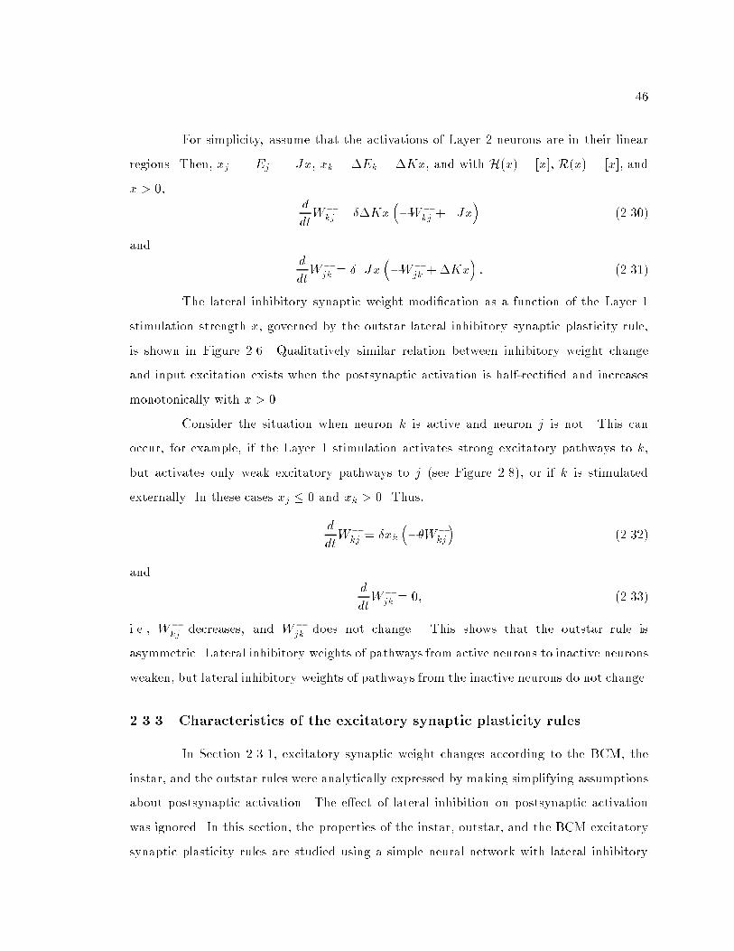
46For simplicity, assume that the activations of Layer 2 neurons are in their linearregions. Then, xj = �Ej = �Jx, xk = �Ek = �Kx, and with H(x) = [x], R(x) = [x], andx > 0, ddtW�kj = ��Kx ��W�kj + �Jx� (2.30)and ddtW�jk = ��Jx ��W�jk +�Kx� : (2.31)The lateral inhibitory synaptic weight modi�cation as a function of the Layer 1stimulation strength x, governed by the outstar lateral inhibitory synaptic plasticity rule,is shown in Figure 2.6. Qualitatively similar relation between inhibitory weight changeand input excitation exists when the postsynaptic activation is half-recti�ed and increasesmonotonically with x > 0.Consider the situation when neuron k is active and neuron j is not. This canoccur, for example, if the Layer 1 stimulation activates strong excitatory pathways to k,but activates only weak excitatory pathways to j (see Figure 2.8), or if k is stimulatedexternally. In these cases xj � 0 and xk > 0. Thus,ddtW�kj = �xk ���W�kj� (2.32)and ddtW�jk = 0; (2.33)i.e., W�kj decreases, and W�jk does not change. This shows that the outstar rule isasymmetric. Lateral inhibitory weights of pathways from active neurons to inactive neuronsweaken, but lateral inhibitory weights of pathways from the inactive neurons do not change.2.3.3 Characteristics of the excitatory synaptic plasticity rulesIn Section 2.3.1, excitatory synaptic weight changes according to the BCM, theinstar, and the outstar rules were analytically expressed by making simplifying assumptionsabout postsynaptic activation. The e�ect of lateral inhibition on postsynaptic activationwas ignored. In this section, the properties of the instar, outstar, and the BCM excitatorysynaptic plasticity rules are studied using a simple neural network with lateral inhibitory

47

0.0 0.2 0.4 0.6 0.8 1.0-0.050.000.050.100.150.200.250.300.350.400.450.50

Input excitation strength

Syn

aptic

pla

stic

ity (

x 0.

1)Outstar inhibitory

Figure 2.6: The outstar inhibitory synaptic plasticity rule under the linearityassumption.The change in synaptic weight as a function of the presynaptic activity according to theoutstar lateral inhibitory synaptic plasticity rule. The rule produces LTP when postsynapticactivation exceeds a variable inhibitory synaptic LTP threshold (a function of the currentsynaptic weight) and LTD when postsynaptic activation is below the variable threshold. Theinhibitory synaptic plasticity under the linearity assumption is governed by Equation 2.29with � = 0:10, � = 1:5, � = 4:0, J = 0:25, K = 0:5, and W�kj = 0:4.

48pathways. Because the activation of model neurons in the network with lateral inhibitioncannot be expressed analytically, the activation equation was solved numerically.If pre- and postsynaptic activations can be controlled independently, the threeexcitatory synaptic plasticity rules give di�erent results. In the following subsections, theproperties of the three rules are studied as a function of presynaptic stimulation strength,and the role of postsynaptic activation in the three rules is explored. Synaptic plasticity instimulated (homosynaptic) and unstimulated (heterosynaptic) pathways is studied.Some experiments have shown dependence of synaptic plasticity on the initialexcitatory synaptic weight. Therefore, the e�ects of the initial synaptic weight on synapticplasticity according to the instar, the outstar, and the BCM excitatory synaptic plasticityrules are analyzed.Finally, associative synaptic plasticity (Brown et al., 1990; Levy & Steward, 1979;Barrionuevo & Brown, 1983; Kelso & Brown, 1986) is modeled using the instar, the outstar,and the BCM excitatory synaptic plasticity rules in the last subsection.The simple neural network used in the simulations is shown in Figure 2.7. Thepostsynaptic neurons a and b receive excitatory inputs from the presynaptic neurons c,d, and e. The postsynaptic neurons a and b inhibit each other via lateral inhibitorypathways. The activation of the postsynaptic neurons a and b in response to activationof the presynaptic neurons c, d, and e is governed by the shunting equation (Equation 2.1).In Appendix A, the behavior of the shunting equation as a function of the various parametersis presented.Synaptic plasticity in excitatory synapses as a function of presynapticstimulation strengthThis section explores excitatory synaptic plasticity as a function of presynapticstimulation to excitatory pathways. First, excitatory synaptic plasticity in the conditionedpathways (homosynaptic plasticity) and in the unconditioned pathways (heterosynapticplasticity) to active postsynaptic neurons are studied based on the three rules. Second,homosynaptic and heterosynaptic plasticity according to the three rules are studied inexcitatory pathways to inactive neurons. Then, the equilibrium weights of conditioned

49AAAAAAAAA

AAAAAAAAAAAA

c d

a b

e

Wdb+

Wcb+Wca

+

Wda+

Web+

Wea+

Wab

Wba

Figure 2.7: Model network.The �gure shows the simple network used in the simulations. W+ij represents the e�cacy ofthe excitatory pathway from neuron i to neuron j, and W�ij represents the e�cacy of theinhibitory pathway from neuron i to neuron j.

50and unconditioned pathways after repeated conditioning stimulations, according to thethree rules, are presented. Finally, some of the e�ects of network interactions on synapticplasticity, according to the three rules, are considered.Synaptic plasticity in pathways to an active neuron. In Figure 2.8, thepresynaptic neuron c was stimulated. The stimulation of neuron c is presented by xc.Figures 2.8a and 2.8b show the activation level of postsynaptic neurons a and b, respectively,as xc was varied from 0 to 1.Synaptic plasticity in the stimulated pathways (homosynaptic plasticity) based onthe three rules as a function of presynaptic stimulation strength is shown in Figure 2.8.Synaptic plasticity in the unstimulated pathways (heterosynaptic plasticity) is also shownin Figure 2.8.In the stimulated pathway from neuron c to active neuron a in Figure 2.8, thethree rules weakened the excitatory synaptic weight W+ca when presynaptic stimulation xcwas weak and strengthened W+ca when xc was strong (Figure 2.8c). In the absence of anypresynaptic stimulation, W+ca did not change according to the three rules (Figure 2.8c).Thus, the instar, the outstar, and the BCM excitatory synaptic plasticity rules can producehomosynaptic LTP and LTD.In the unstimulated excitatory pathways to neuron a, e.g., from neuron d, only LTDwas produced by the instar excitatory synaptic plasticity rule, because the synaptic weightW+da was greater than the activation level of neuron d, xd, which was zero (Figure 2.8e).As xc was increased, W+da decreased more (Figure 2.8e). This happened because in theinstar rule the magnitude of change in excitatory synaptic weight is proportional to thepostsynaptic activation, and xa increased with xc (Figure 2.8a). According to the outstarand the BCM excitatory synaptic plasticity rules, presynaptic activation is required for thelearning rules to be enabled (Equations 2.4 and 2.9). Thus, in the unstimulated pathwaysno synaptic plasticity occurred (Figure 2.8e).In Figure 2.8c, the amount of LTD produced by the outstar and the BCM rules wassmall, because of the simulation parameters. For comparison, a simulation with a di�erentset of parameters was run, to produce larger LTD (Figure 2.9c). In Figure 2.9, the initialweight of the stimulated pathway ca was increased, and the learning rate parameters � and

510.0 0.2 0.4 0.6 0.8 1.0

-0.20

0.00

0.20

0.40

0.60

0.80

1.00

Presynaptic stimulation strength(a)

Act

ivat

ion

Neuron a

0.0 0.2 0.4 0.6 0.8 1.0-0.20

0.00

0.20

0.40

0.60

0.80

1.00

Presynaptic stimulation strength(b)

Act

ivat

ion

Neuron b

0.0 0.2 0.4 0.6 0.8 1.0-0.20

-0.10

0.00

0.10

0.20

Presynaptic stimulation strength(c)

Syn

aptic

pla

stic

ity (

x 0.

1)

Instar excitatory

0.0 0.2 0.4 0.6 0.8 1.0-0.20

-0.10

0.00

0.10

0.20

Presynaptic stimulation strength(e)

Syn

aptic

pla

stic

ity (

x 0.

1)

Instar excitatory

0.0 0.2 0.4 0.6 0.8 1.0-0.20

-0.10

0.00

0.10

0.20

Presynaptic stimulation strength(d)

Syn

aptic

pla

stic

ity (

x 0.

1)

Instar excitatory

0.0 0.2 0.4 0.6 0.8 1.0-0.20

-0.10

0.00

0.10

0.20

Presynaptic stimulation strength(f)

Syn

aptic

pla

stic

ity (

x 0.

1)

Instar excitatory

0.0 0.2 0.4 0.6 0.8 1.0-0.20

-0.10

0.00

0.10

0.20

Presynaptic stimulation strength(c)

Syn

aptic

pla

stic

ity (

x 0.

1)

Outstar excitatory

0.0 0.2 0.4 0.6 0.8 1.0-0.20

-0.10

0.00

0.10

0.20

Presynaptic stimulation strength(e)

Syn

aptic

pla

stic

ity (

x 0.

1)

Outstar excitatory

0.0 0.2 0.4 0.6 0.8 1.0-0.20

-0.10

0.00

0.10

0.20

Presynaptic stimulation strength(d)

Syn

aptic

pla

stic

ity (

x 0.

1)

Outstar excitatory

0.0 0.2 0.4 0.6 0.8 1.0-0.20

-0.10

0.00

0.10

0.20

Presynaptic stimulation strength(f)

Syn

aptic

pla

stic

ity (

x 0.

1)

Outstar excitatory

0.0 0.2 0.4 0.6 0.8 1.0-0.20

-0.10

0.00

0.10

0.20

Presynaptic stimulation strength(c)

Syn

aptic

pla

stic

ity (

x 0.

1)

BCM

0.0 0.2 0.4 0.6 0.8 1.0-0.20

-0.10

0.00

0.10

0.20

Presynaptic stimulation strength(e)

Syn

aptic

pla

stic

ity (

x 0.

1)

BCM

0.0 0.2 0.4 0.6 0.8 1.0-0.20

-0.10

0.00

0.10

0.20

Presynaptic stimulation strength(d)

Syn

aptic

pla

stic

ity (

x 0.

1)BCM

0.0 0.2 0.4 0.6 0.8 1.0-0.20

-0.10

0.00

0.10

0.20

Presynaptic stimulation strength(f)

Syn

aptic

pla

stic

ity (

x 0.

1)

BCM

Figure 2.8: Legend on next page.

52Figure 2.8: Simulation results: Changes in excitatory synaptic e�cacy ofstimulated and unstimulated pathways as a function of presynaptic stimulationstrength.Figure on previous page. The synaptic weight changes are shown according to the threerules after activating neuron c; the activation level of neuron c of Figure 2.7, xc, was variedfrom 0 to 1. Panels (a) and (b) show the activation of neurons a and b, respectively, as xcwas varied, (c) and (d) show plasticity in the stimulated pathways from neuron c to neuron aand from neuron c to neuron b, respectively, as xc was varied, and (e) and (f) show plasticityin the unstimulated pathways from neuron d to neuron a and from neuron d to neuron b,respectively, as xc was varied. The rate of weight change in the instar rule became zerowhen postsynaptic activation was suppressed (d), (f). The rate of weight change in theoutstar rule became zero when presynaptic activation was suppressed (e), (f). The rate ofweight change in the BCM rule became zero when either pre- or postsynaptic activationwas suppressed (d), (e), (f). In this simulation the initial synaptic pathway weights in thenetwork shown in Figure 2.4 were assigned as follows: W+ca = 0:5, W+cb = 0:25, W+da = 0:4,W+db = 0:4, W+ea = 0:25, W+eb = 0:5, W�ab = W�ba = 0:4. The parameters for the activationequation (Equation 2.1) were A = 0:1, B = 1, C = 0:05, � = 1, and = 15. The activationlevel was computed using the Euler method with a time step of 0.04 until t = 40. Theinitial activation level of neurons a and b was set to zero. The parameters for the instarexcitatory synaptic plasticity rule were � = 0:05, F(x) = [x], and P(x) = [x], for the outstarexcitatory synaptic plasticity rule were � = 0:05, G(x) = [x], and Q(x) = [x], and for theBCM rule were � = 0:05, and �a = �b = 0:5.� for the outstar and the BCM rules, respectively, were increased. For the BCM rule, theinitial LTP threshold for neuron a was also increased. The magnitude of weight changeincreased with increase in the learning rate parameters. In addition, increasing the initialweight increased the magnitude of the di�erence between the postsynaptic activation andthe initial weight and therefore increased the magnitude of weight change according tothe outstar rule. Increasing the LTP threshold increased the magnitude of the di�erencebetween the postsynaptic activation and the LTP threshold and therefore increased themagnitude of weight change according to the BCM rule.Synaptic plasticity in pathways to an inactive neuron. In Figure 2.8bd, thestimulated excitatory pathway from neuron c to inactive neuron b did not undergo synapticplasticity under the instar excitatory synaptic plasticity rule because neuron b was inactive.The outstar excitatory synaptic plasticity rule produced LTD in the excitatory pathwayfrom neuron c to neuron b because neuron b was inactive. Under the BCM excitatory

530.0 0.2 0.4 0.6 0.8 1.0

-0.20

0.00

0.20

0.40

0.60

0.80

1.00

Presynaptic stimulation strength(a)

Act

ivat

ion

Neuron a

0.0 0.2 0.4 0.6 0.8 1.0-0.20

0.00

0.20

0.40

0.60

0.80

1.00

Presynaptic stimulation strength(b)

Act

ivat

ion

Neuron b

0.0 0.2 0.4 0.6 0.8 1.0-0.40

-0.30

-0.20

-0.10

0.00

0.10

0.20

0.30

0.40

Presynaptic stimulation strength(c)

Syn

aptic

pla

stic

ity (

x 0.

1)

Instar excitatory

0.0 0.2 0.4 0.6 0.8 1.0-0.40

-0.30

-0.20

-0.10

0.00

0.10

0.20

0.30

0.40

Presynaptic stimulation strength(e)

Syn

aptic

pla

stic

ity (

x 0.

1)

Instar excitatory

0.0 0.2 0.4 0.6 0.8 1.0-0.40

-0.30

-0.20

-0.10

0.00

0.10

0.20

0.30

0.40

Presynaptic stimulation strength(d)

Syn

aptic

pla

stic

ity (

x 0.

1)

Instar excitatory

0.0 0.2 0.4 0.6 0.8 1.0-0.40

-0.30

-0.20

-0.10

0.00

0.10

0.20

0.30

0.40

Presynaptic stimulation strength(f)

Syn

aptic

pla

stic

ity (

x 0.

1)

Instar excitatory

0.0 0.2 0.4 0.6 0.8 1.0-0.40

-0.30

-0.20

-0.10

0.00

0.10

0.20

0.30

0.40

Presynaptic stimulation strength(c)

Syn

aptic

pla

stic

ity (

x 0.

1)

Outstar excitatory

0.0 0.2 0.4 0.6 0.8 1.0-0.40

-0.30

-0.20

-0.10

0.00

0.10

0.20

0.30

0.40

Presynaptic stimulation strength(e)

Syn

aptic

pla

stic

ity (

x 0.

1)

Outstar excitatory

0.0 0.2 0.4 0.6 0.8 1.0-0.40

-0.30

-0.20

-0.10

0.00

0.10

0.20

0.30

0.40

Presynaptic stimulation strength(d)

Syn

aptic

pla

stic

ity (

x 0.

1)

Outstar excitatory

0.0 0.2 0.4 0.6 0.8 1.0-0.40

-0.30

-0.20

-0.10

0.00

0.10

0.20

0.30

0.40

Presynaptic stimulation strength(f)

Syn

aptic

pla

stic

ity (

x 0.

1)

Outstar excitatory

0.0 0.2 0.4 0.6 0.8 1.0-0.40

-0.30

-0.20

-0.10

0.00

0.10

0.20

0.30

0.40

Presynaptic stimulation strength(c)

Syn

aptic

pla

stic

ity (

x 0.

1)

BCM

0.0 0.2 0.4 0.6 0.8 1.0-0.40

-0.30

-0.20

-0.10

0.00

0.10

0.20

0.30

0.40

Presynaptic stimulation strength(e)

Syn

aptic

pla

stic

ity (

x 0.

1)

BCM

0.0 0.2 0.4 0.6 0.8 1.0-0.40

-0.30

-0.20

-0.10

0.00

0.10

0.20

0.30

0.40

Presynaptic stimulation strength(d)

Syn

aptic

pla

stic

ity (

x 0.

1)BCM

0.0 0.2 0.4 0.6 0.8 1.0-0.40

-0.30

-0.20

-0.10

0.00

0.10

0.20

0.30

0.40

Presynaptic stimulation strength(f)

Syn

aptic

pla

stic

ity (

x 0.

1)

BCM

Figure 2.9: Legend on next page.

54Figure 2.9: Simulation results: Changes in excitatory synaptic e�cacy ofstimulated and unstimulated pathways under faster learning parameters.Figure on previous page. See Figure 2.8 for conventions. There was no synaptic weightchange under the instar rule in (d,f), under the outstar rule (e,f), and under the BCMrule (d,e,f). In this simulation the initial synaptic pathway weights in the network shownin Figure 2.4 were assigned as follows: W+ca = 0:8, W+cb = 0:25, W+da = 0:4, W+db = 0:4,W+ea = 0:25, W+eb = 0:8, W�ab = W�ba = 0:4. The parameters for the activation equation(Equation 2.1) were A = 0:1, B = 1, C = 0:05, � = 1, and = 15. The activation levelwas computed using the Euler method with a time step of 0.04 until t = 40. The initialactivation of neurons a and b was set to zero. The parameters for the instar excitatorysynaptic plasticity rule were � = 0:02, F(x) = [x], and P(x) = [x], for the outstar excitatorysynaptic plasticity rule were � = 0:15, G(x) = [x], and Q(x) = [x], and for the BCM rulewere � = 0:15, and �a = �b = 0:8. The parameter values in boldface di�er from the valuesused in the simulations for Figure 2.8.synaptic plasticity rule, no plasticity was observed because neuron b was inactive.In the unstimulated excitatory pathways to the inactive neuron b, e.g., fromneuron d, no plasticity was produced in W+db because xb � 0 (Figure 2.8f). Under theoutstar excitatory and the BCM synaptic plasticity rules, presynaptic activation is requiredfor the plasticity to be enabled (Equations 2.4 and 2.9). Thus, in the unstimulated pathwaysno synaptic plasticity occurred.Under the instar excitatory synaptic plasticity rule, the stimulated pathway canbe potentiated or depressed; however, the unstimulated pathways can only weaken, or atbest, remain constant. Under the outstar excitatory synaptic plasticity rule, the stimulatedpathways may be potentiated or depressed, and unstimulated pathways do not undergosynaptic plasticity. The BCM rule also potentiates or depresses the stimulated pathwaysonto a postsynaptic neuron and does not modify synaptic weight of unstimulated pathways.Equilibrium values of synaptic weights. In this section, changes in the weights ofexcitatory pathways according to the three excitatory synaptic plasticity rules are studiedwhen an excitatory pathway is continuously stimulated.According to the instar excitatory synaptic plasticity rule, the synaptic weightW+caequilibrates to a value proportional to a function, P(), of the presynaptic stimulationstrength xc (Grossberg, 1982; see Figure 2.10ce). The weight change in W+ca approacheszero as W+ca approaches P(xa), and for P(xd(t)) = 0 weight change in W+da approaches zero

55as W+da approaches zero.The outstar excitatory synaptic plasticity rule causes the synaptic weight W+ca toequilibrate at a value proportional to a function, Q(), of the postsynaptic activation xa(see Figure 2.10ce); the weight change of W+ca approaches zero as W+ca approaches Q(xa),and for Q(xb) = 0 the weight change of W+cb approaches zero as W+cb approaches zero.On the other hand, the synaptic weight W+ca may not equilibrate when synapticplasticity is governed by the BCM rule (Figures 2.10 and 2.11). In Figure 2.10, stimulatingneuron c with xc = 1 activates neuron a, which suppresses neuron b. In this WTA case,xa = �BW+caxcA+�W+caxc at equilibrium in response to xc according to Equation 2.1 because xb � 0.In the simulation in Figure 2.10, �a(t) < xa(t) for t � 0 (Figure 2.10a), and W+ca increasesunder the BCM rule. According to the BCM rule, W+ca equilibrates at some time t0, if�a(t0) = [xa(t0)], and �a(t) = �a(t + 1) for t � t0. With p = 2 and c0 = 1, �a(t) = �a(t + 1)implies that �a(t) = [xa(t)]2 according to the approximation for the BCM LTP thresholdmodi�cation (Equation 2.7), and �a(t) = [xa(t)]2, when �a(t) = [xa(t)] = 1, or when�a(t) = [xa(t)] = 0. But, xa = �BW+caxcA+�W+caxc < B = 1 (for the parameters in Figure 2.10), andxa approaches 1 as W+ca approaches 1. Thus, for the parameters used in Figure 2.10, theBCM rule caused W+ca to increase without bound. Since neuron b remained inactive, W+cb ,the weight of the stimulated pathway from neuron c to neuron b did not change, and �bdecayed to 0 according to the BCM rule (Figure 2.10d).Figure 2.11 shows changes in weights of stimulated excitatory pathways accordingto the BCM rule using several di�erent parameters. The curves labeled \Initial LTPthreshold = 1" show weight changes when the initial LTP thresholds of neurons a and bwere 1 and were greater than xa(0) and xb(0), respectively. Since the activation of neuron awas less than 1, W+ca increased without bound (Figure 2.11e).When xa was allowed to become equal to 1, for example, when the decay parameterin the activation equation was set to 0, the BCM rule with p = 2 and c0 = 1 caused W+ca toreach an equilibrium value (curves labeled \A = 0" in Figure 2.11eg). When the parameterA in Equation 2.1 is set to zero, under WTA conditions xa = B = 1 (Figure 2.11a), and �aequilibrated at 1 (Figure 2.11c).The BCM rule causes the weights to reach stable values if p is set to 1. According

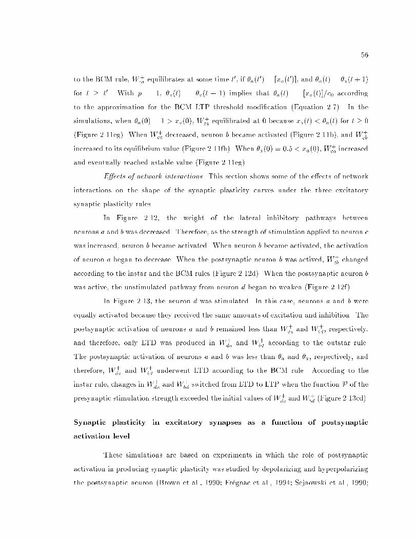
56to the BCM rule, W+ca equilibrates at some time t0, if �a(t0) = [xa(t0)], and �a(t) = �a(t+ 1)for t � t0. With p = 1, �a(t) = �a(t + 1) implies that �a(t) = [xa(t)]=c0 accordingto the approximation for the BCM LTP threshold modi�cation (Equation 2.7). In thesimulations, when �a(0) = 1 > xa(0), W+ca equilibrated at 0 because xa(t) < �a(t) for t � 0(Figure 2.11eg). When W+ca decreased, neuron b became activated (Figure 2.11b), and W+cbincreased to its equilibrium value (Figure 2.11fh). When �a(0) = 0:5 < xa(0),W+ca increasedand eventually reached astable value (Figure 2.11eg).E�ects of network interactions. This section shows some of the e�ects of networkinteractions on the shape of the synaptic plasticity curves under the three excitatorysynaptic plasticity rules.In Figure 2.12, the weight of the lateral inhibitory pathways betweenneurons a and b was decreased. Therefore, as the strength of stimulation applied to neuron cwas increased, neuron b became activated. When neuron b became activated, the activationof neuron a began to decrease. When the postsynaptic neuron b was actived, W+cb changedaccording to the instar and the BCM rules (Figure 2.12d). When the postsynaptic neuron bwas active, the unstimulated pathway from neuron d began to weaken (Figure 2.12f).In Figure 2.13, the neuron d was stimulated. In this case, neurons a and b wereequally activated because they received the same amounts of excitation and inhibition. Thepostsynaptic activation of neurons a and b remained less than W+da and W+bd, respectively,and therefore, only LTD was produced in W+da and W+bd according to the outstar rule.The postsynaptic activation of neurons a and b was less than �a and �a, respectively, andtherefore, W+da and W+bd underwent LTD according to the BCM rule. According to theinstar rule, changes in W+da and W+bd switched from LTD to LTP when the function P of thepresynaptic stimulation strength exceeded the initial values ofW+da andW+bd (Figure 2.13cd).Synaptic plasticity in excitatory synapses as a function of postsynapticactivation levelThese simulations are based on experiments in which the role of postsynapticactivation in producing synaptic plasticity was studied by depolarizing and hyperpolarizingthe postsynaptic neuron (Brown et al., 1990; Fr�egnac et al., 1994; Sejnowski et al., 1990;

570 50 100 150 200

-0.20

0.00

0.20

0.40

0.60

0.80

1.00

Number of iterations(a)

Act

ivat

ion

or B

CM

LT

P th

resh

old

Instar excitatory

0 50 100 150 200-0.20

0.00

0.20

0.40

0.60

0.80

1.00

Number of iterations(a)

Act

ivat

ion

or B

CM

LT

P th

resh

old

Outstar excitatory

0 50 100 150 200-0.20

0.00

0.20

0.40

0.60

0.80

1.00

Number of iterations(a)

Act

ivat

ion

or B

CM

LT

P th

resh

old BCM

0 50 100 150 200-0.20

0.00

0.20

0.40

0.60

0.80

1.00

Number of iterations(a)

Act

ivat

ion

or B

CM

LT

P th

resh

old

BCM LTP threshold

0 50 100 150 200-0.20

0.00

0.20

0.40

0.60

0.80

1.00

Number of iterations(b)

Act

ivat

ion

or B

CM

LT

P th

resh

old

Instar excitatory

0 50 100 150 200-0.20

0.00

0.20

0.40

0.60

0.80

1.00

Number of iterations(b)

Act

ivat

ion

or B

CM

LT

P th

resh

old

Outstar excitatory

0 50 100 150 200-0.20

0.00

0.20

0.40

0.60

0.80

1.00

Number of iterations(b)

Act

ivat

ion

or B

CM

LT

P th

resh

old BCM

0 50 100 150 200-0.20

0.00

0.20

0.40

0.60

0.80

1.00

Number of iterations(b)

Act

ivat

ion

or B

CM

LT

P th

resh

old

BCM LTP threshold

0 50 100 150 2000.00

0.50

1.00

1.50

Number of iterations(c)

Syn

aptic

str

engt

h (x

0.1

)

Instar excitatory - pathway ca

0 50 100 150 2000.00

0.50

1.00

1.50

Number of iterations(d)

Syn

aptic

str

engt

h (x

0.1

)

Instar excitatory - pathway da

0 50 100 150 2000.00

0.50

1.00

1.50

Number of iterations(c)

Syn

aptic

str

engt

h (x

0.1

)

Outstar excitatory - pathway ca

0 50 100 150 2000.00

0.50

1.00

1.50

Number of iterations(d)

Syn

aptic

str

engt

h (x

0.1

)Outstar excitatory - pathway cb

0 50 100 150 2000.00

0.50

1.00

1.50

Number of iterations(c)

Syn

aptic

str

engt

h (x

0.1

) BCM - pathway ca

0 50 100 150 2000.00

0.50

1.00

1.50

Number of iterations(d)

Syn

aptic

str

engt

h (x

0.1

) BCM - pathway cb

0 50 100 150 200-0.20

-0.10

0.00

0.10

0.20

Number of iterations(e)

Rat

e of

syn

aptic

pla

stic

ity (

x 0.

1)

Instar excitatory - pathway ca

0 50 100 150 200-0.20

-0.10

0.00

0.10

0.20

Number of iterations(f)

Rat

e of

syn

aptic

pla

stic

ity (

x 0.

1)

Instar excitatory - pathway da

0 50 100 150 200-0.20

-0.10

0.00

0.10

0.20

Number of iterations(e)

Rat

e of

syn

aptic

pla

stic

ity (

x 0.

1) Outstar excitatory - pathway ca

0 50 100 150 200-0.20

-0.10

0.00

0.10

0.20

Number of iterations(f)

Rat

e of

syn

aptic

pla

stic

ity (

x 0.

1) Outstar excitatory - pathway cb

0 50 100 150 200-0.20

-0.10

0.00

0.10

0.20

Number of iterations(e)

Rat

e of

syn

aptic

pla

stic

ity (

x 0.

1)

BCM - pathway ca

0 50 100 150 200-0.20

-0.10

0.00

0.10

0.20

Number of iterations(f)

Rat

e of

syn

aptic

pla

stic

ity (

x 0.

1)

BCM - pathway cb

Figure 2.10: Legend on next page.

58Figure 2.10: Simulation results: Equilibrium values of excitatory synaptic e�cacyof stimulated and unstimulated pathways.Figure on previous page. The simulation parameters were the same as those in Figure 2.8.In this simulation, presynaptic stimulation was applied by keeping xc �xed at 1 for200 iterations. The synaptic weights were changed every iteration. Panels (a) and (b)show the activation level of neurons a and b, respectively, over a period of 200 iterations asthe excitatory synaptic weights change. In the case of the BCM rule, panels (a) and (b) alsoshow the LTP threshold of neurons a and b, respectively. The LTP threshold for the instarand the outstar excitatory synaptic plasticity rules are the excitatory synaptic weight itself.Panels (c) and (d) show the excitatory synaptic weight of di�erent excitatory pathways,and panels (e) and (f) show the rate of excitatory synaptic weight change in the di�erentexcitatory pathways. The pathway from neuron i to neuron j is labeled pathway ij. Inthe simulations, p = 2, � = 20, and c0 = 1. In the simulations, activation of neuron bwas suppressed (b), and therefore the weight of the excitatory pathway from neuron c toneuron b did not change under the BCM rule (d,f).Stanton & Sejnowski, 1989).In the simulations, a presynaptic element was stimulated at a �xed level,e.g., neuron c was stimulated at xc > 0, and the activation level of a postsynapticneuron, e.g., that of neuron a, xa, was varied independently.The instar excitatory synaptic plasticity rule increased the magnitude of changein W+ca as xa was increased (Figure 2.14a); however, the sign of change in W+ca remainedthe same because it depends on the sign of (�W+ca + P(xc)) (Figure 2.14a), which was�xed for �xed initial W+ca and P(xc). Furthermore, synaptic plasticity was disabled whenpostsynaptic activation was zero (Figure 2.14a). When the postsynaptic activation ofneuron a, xa, was kept �xed and presynaptic activation of neuron c, xc, was varied from0 to 1 in Figure 2.14b, the synaptic plasticity in W+ca went from LTD to LTP; for highervalues of xa the rate of plasticity increased. Thus, according to the instar excitatorysynaptic plasticity rule, postsynaptic activation is required to enable plasticity, postsynapticactivation a�ects the rate of plasticity, and postsynaptic activation does not a�ect the signof plasticity (the sign of plasticity depends on presynaptic activation and the weight).According to the outstar excitatory synaptic plasticity rule, the sign of change inW+ca depended on the postsynaptic activation; as xa was increased when xc > 0 was kept�xed, the change in W+ca went from depression to potentiation (Figure 2.14c). In the outstar

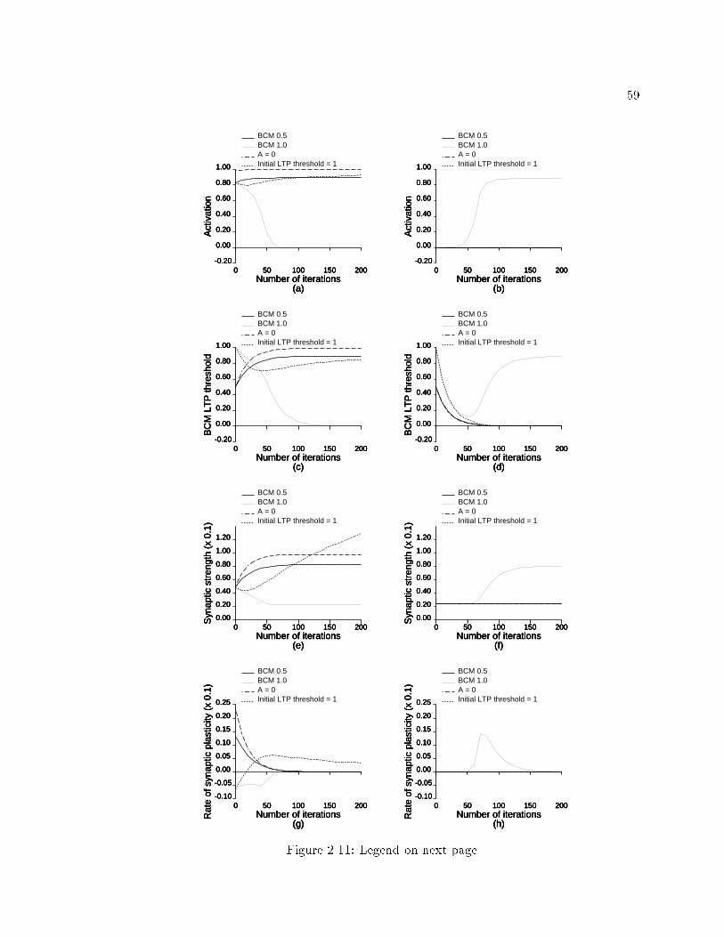
590 50 100 150 200

-0.20

0.00

0.20

0.40

0.60

0.80

1.00

Number of iterations(a)

Act

ivat

ion

BCM 0.5

0 50 100 150 200-0.20

0.00

0.20

0.40

0.60

0.80

1.00

Number of iterations(b)

Act

ivat

ion

BCM 0.5

0 50 100 150 200-0.20

0.00

0.20

0.40

0.60

0.80

1.00

Number of iterations(a)

Act

ivat

ion

BCM 1.0

0 50 100 150 200-0.20

0.00

0.20

0.40

0.60

0.80

1.00

Number of iterations(b)

Act

ivat

ion

BCM 1.0

0 50 100 150 200-0.20

0.00

0.20

0.40

0.60

0.80

1.00

Number of iterations(a)

Act

ivat

ion

A = 0

0 50 100 150 200-0.20

0.00

0.20

0.40

0.60

0.80

1.00

Number of iterations(b)

Act

ivat

ion

A = 0

0 50 100 150 200-0.20

0.00

0.20

0.40

0.60

0.80

1.00

Number of iterations(a)

Act

ivat

ion

Initial LTP threshold = 1

0 50 100 150 200-0.20

0.00

0.20

0.40

0.60

0.80

1.00

Number of iterations(b)

Act

ivat

ion

Initial LTP threshold = 1

0 50 100 150 200-0.20

0.00

0.20

0.40

0.60

0.80

1.00

Number of iterations(c)

BC

M L

TP

thre

shol

d

BCM 0.5

0 50 100 150 200-0.20

0.00

0.20

0.40

0.60

0.80

1.00

Number of iterations(d)

BC

M L

TP

thre

shol

d

BCM 0.5

0 50 100 150 200-0.20

0.00

0.20

0.40

0.60

0.80

1.00

Number of iterations(c)

BC

M L

TP

thre

shol

d

BCM 1.0

0 50 100 150 200-0.20

0.00

0.20

0.40

0.60

0.80

1.00

Number of iterations(d)

BC

M L

TP

thre

shol

d

BCM 1.0

0 50 100 150 200-0.20

0.00

0.20

0.40

0.60

0.80

1.00

Number of iterations(c)

BC

M L

TP

thre

shol

d

A = 0

0 50 100 150 200-0.20

0.00

0.20

0.40

0.60

0.80

1.00

Number of iterations(d)

BC

M L

TP

thre

shol

d

A = 0

0 50 100 150 200-0.20

0.00

0.20

0.40

0.60

0.80

1.00

Number of iterations(c)

BC

M L

TP

thre

shol

d

Initial LTP threshold = 1

0 50 100 150 200-0.20

0.00

0.20

0.40

0.60

0.80

1.00

Number of iterations(d)

BC

M L

TP

thre

shol

d

Initial LTP threshold = 1

0 50 100 150 2000.00

0.20

0.40

0.60

0.80

1.00

1.20

Number of iterations(e)

Syn

aptic

str

engt

h (x

0.1

)

BCM 0.5

0 50 100 150 2000.00

0.20

0.40

0.60

0.80

1.00

1.20

Number of iterations(f)

Syn

aptic

str

engt

h (x

0.1

)

BCM 0.5

0 50 100 150 2000.00

0.20

0.40

0.60

0.80

1.00

1.20

Number of iterations(e)

Syn

aptic

str

engt

h (x

0.1

)

BCM 1.0

0 50 100 150 2000.00

0.20

0.40

0.60

0.80

1.00

1.20

Number of iterations(f)

Syn

aptic

str

engt

h (x

0.1

)

BCM 1.0

0 50 100 150 2000.00

0.20

0.40

0.60

0.80

1.00

1.20

Number of iterations(e)

Syn

aptic

str

engt

h (x

0.1

)

A = 0

0 50 100 150 2000.00

0.20

0.40

0.60

0.80

1.00

1.20

Number of iterations(f)

Syn

aptic

str

engt

h (x

0.1

)

A = 0

0 50 100 150 2000.00

0.20

0.40

0.60

0.80

1.00

1.20

Number of iterations(e)

Syn

aptic

str

engt

h (x

0.1

) Initial LTP threshold = 1

0 50 100 150 2000.00

0.20

0.40

0.60

0.80

1.00

1.20

Number of iterations(f)

Syn

aptic

str

engt

h (x

0.1

) Initial LTP threshold = 1

0 50 100 150 200-0.10

-0.05

0.00

0.05

0.10

0.15

0.20

0.25

Number of iterations(g)

Rat

e of

syn

aptic

pla

stic

ity (

x 0.

1)

BCM 0.5

0 50 100 150 200-0.10

-0.05

0.00

0.05

0.10

0.15

0.20

0.25

Number of iterations(h)

Rat

e of

syn

aptic

pla

stic

ity (

x 0.

1)

BCM 0.5

0 50 100 150 200-0.10

-0.05

0.00

0.05

0.10

0.15

0.20

0.25

Number of iterations(g)

Rat

e of

syn

aptic

pla

stic

ity (

x 0.

1)

BCM 1.0

0 50 100 150 200-0.10

-0.05

0.00

0.05

0.10

0.15

0.20

0.25

Number of iterations(h)

Rat

e of

syn

aptic

pla

stic

ity (

x 0.

1)

BCM 1.0

0 50 100 150 200-0.10

-0.05

0.00

0.05

0.10

0.15

0.20

0.25

Number of iterations(g)

Rat

e of

syn

aptic

pla

stic

ity (

x 0.

1) A = 0

0 50 100 150 200-0.10

-0.05

0.00

0.05

0.10

0.15

0.20

0.25

Number of iterations(h)

Rat

e of

syn

aptic

pla

stic

ity (

x 0.

1) A = 0

0 50 100 150 200-0.10

-0.05

0.00

0.05

0.10

0.15

0.20

0.25

Number of iterations(g)

Rat

e of

syn

aptic

pla

stic

ity (

x 0.

1)

Initial LTP threshold = 1

0 50 100 150 200-0.10

-0.05

0.00

0.05

0.10

0.15

0.20

0.25

Number of iterations(h)

Rat

e of

syn

aptic

pla

stic

ity (

x 0.

1)

Initial LTP threshold = 1

Figure 2.11: Legend on next page.

60Figure 2.11: Simulation results: Equilibrium values of excitatory synaptic e�cacyof stimulated and unstimulated pathways according to the BCM rule.Figure on previous page. The relationship between �j and xj and their e�ect on synapticplasticity are shown. The initial network weights and the BCM excitatory synaptic plasticityrule parameters are given in Figure 2.8. As in Figure 2.12, neuron c is activated at a �xedlevel of 1 for 200 iterations. Panels (a) and (b) show the activation level of neurons a andb, respectively. In the curves labeled \BCM 0.5," the BCM LTP threshold modi�cationfunction parameters were p = 1, c0 = 1, and � = 20, the activation equation parameterswere the same as in Figure 2.8, and the initial LTP thresholds for neurons a and b were�a = �b = 0:5. In the curves labeled \BCM 1.0," the parameters were the same, exceptthat �a = �b = 1:0. In the curves labeled \A = 0," the decay parameter A in the activationequation was set to 0, and the other activation equation parameters were the same as inFigure 2.8, �a(0) = �b(0) = 0:5, and the LTP threshold was varied as in Figure 2.12. In thecurves labeled \Initial LTP threshold = 1," the initial LTP thresholds for neurons a and bwere set to 1, the activation equation parameters were the same as in Figure 2.8, and theLTP threshold was varied as in Figure 2.12. Panels (c) and (d) show the LTP threshold ofneurons a and b, respectively. Panel (e) shows W+ca, and panel (g) shows the rate of changein W+ca. Panel (f) shows W+cb , and panel (h) shows the rate of change in W+cb . In the curveslabeled \BCM 0.5," \A = 0," and \Initial LTP threshold = 1," the activation of neuron bwas suppressed (b), and thereforeW+cb did not change under the BCM rule (f,h). The curveslabeled \BCM 0.5," \A = 0," and \Initial LTP threshold = 1," are overlapping in (f,h).In (d), the curves labeled \BCM 0.5" and \A = 0," are overlapping.rule, the sign of weight change depends on the sign of (�W+ca +Q(xa)), and the magnitudeof weight change in W+ca is a�ected by the magnitude of (�W+ca + Q(xa)). The magnitudeof weight change also depended on the presynaptic activation level (Figure 2.14cd); as thepresynaptic activation xc was increased, the magnitude of synaptic weight change increased.When the postsynaptic activation xa was �xed and presynaptic activation xc was varied,the magnitude of weight change in Wca increased, but the sign of weight change was �xed(Figure 2.14d). According to the outstar rule, synaptic weight change did not occur whenthe presynaptic activation was zero (Figure 2.14d). According to the outstar excitatorysynaptic plasticity rule, postsynaptic activation a�ects both the sign of plasticity and themagnitude of weight change.In the BCM excitatory synaptic plasticity rule, the sign of change in W+cadepended on the postsynaptic activation level. As xa was increased with �xed xc > 0,the change in W+ca was zero when xa = 0, W+ca underwent depression when 0 < xa < �a

610.0 0.2 0.4 0.6 0.8 1.0

-0.20

0.00

0.20

0.40

0.60

0.80

1.00

Presynaptic stimulation strength(a)

Act

ivat

ion

Neuron a

0.0 0.2 0.4 0.6 0.8 1.0-0.20

0.00

0.20

0.40

0.60

0.80

1.00

Presynaptic stimulation strength(b)

Act

ivat

ion

Neuron b

0.0 0.2 0.4 0.6 0.8 1.0-0.20

-0.15

-0.10

-0.05

0.00

0.05

0.10

0.15

0.20

Presynaptic stimulation strength(c)

Syn

aptic

pla

stic

ity (

x 0.

1)

Instar excitatory

0.0 0.2 0.4 0.6 0.8 1.0-0.20

-0.15

-0.10

-0.05

0.00

0.05

0.10

0.15

0.20

Presynaptic stimulation strength(e)

Syn

aptic

pla

stic

ity (

x 0.

1)

Instar excitatory

0.0 0.2 0.4 0.6 0.8 1.0-0.20

-0.15

-0.10

-0.05

0.00

0.05

0.10

0.15

0.20

Presynaptic stimulation strength(d)

Syn

aptic

pla

stic

ity (

x 0.

1)

Instar excitatory

0.0 0.2 0.4 0.6 0.8 1.0-0.20

-0.15

-0.10

-0.05

0.00

0.05

0.10

0.15

0.20

Presynaptic stimulation strength(f)

Syn

aptic

pla

stic

ity (

x 0.

1)

Instar excitatory

0.0 0.2 0.4 0.6 0.8 1.0-0.20

-0.15

-0.10

-0.05

0.00

0.05

0.10

0.15

0.20

Presynaptic stimulation strength(c)

Syn

aptic

pla

stic

ity (

x 0.

1)

Outstar excitatory

0.0 0.2 0.4 0.6 0.8 1.0-0.20

-0.15

-0.10

-0.05

0.00

0.05

0.10

0.15

0.20

Presynaptic stimulation strength(e)

Syn

aptic

pla

stic

ity (

x 0.

1)

Outstar excitatory

0.0 0.2 0.4 0.6 0.8 1.0-0.20

-0.15

-0.10

-0.05

0.00

0.05

0.10

0.15

0.20

Presynaptic stimulation strength(d)

Syn

aptic

pla

stic

ity (

x 0.

1)

Outstar excitatory

0.0 0.2 0.4 0.6 0.8 1.0-0.20

-0.15

-0.10

-0.05

0.00

0.05

0.10

0.15

0.20

Presynaptic stimulation strength(f)

Syn

aptic

pla

stic

ity (

x 0.

1)

Outstar excitatory

0.0 0.2 0.4 0.6 0.8 1.0-0.20

-0.15

-0.10

-0.05

0.00

0.05

0.10

0.15

0.20

Presynaptic stimulation strength(c)

Syn

aptic

pla

stic

ity (

x 0.

1)

BCM

0.0 0.2 0.4 0.6 0.8 1.0-0.20

-0.15

-0.10

-0.05

0.00

0.05

0.10

0.15

0.20

Presynaptic stimulation strength(e)

Syn

aptic

pla

stic

ity (

x 0.

1)

BCM

0.0 0.2 0.4 0.6 0.8 1.0-0.20

-0.15

-0.10

-0.05

0.00

0.05

0.10

0.15

0.20

Presynaptic stimulation strength(d)

Syn

aptic

pla

stic

ity (

x 0.

1)BCM

0.0 0.2 0.4 0.6 0.8 1.0-0.20

-0.15

-0.10

-0.05

0.00

0.05

0.10

0.15

0.20

Presynaptic stimulation strength(f)

Syn

aptic

pla

stic

ity (

x 0.

1)

BCM

Figure 2.12: Legend on next page.

62Figure 2.12: Simulation results: The e�ects of lateral inhibitory weight onexcitatory synaptic plasticity.Figure on previous page. In these simulations, all the parameters are the same as inFigure 2.8 except that W�ab = W�ba = 0:2, i.e., the lateral inhibitory weights are weakened.Weakening the lateral inhibitory weights causes neuron b to be activated when inputexcitation was strong (b). See Figure 2.8 for conventions. There was no synaptic weightchange under the instar rule (d,f) when neuron b was inactive. There was no synaptic weightchange under the outstar rule (e,f) and under the BCM rule (d,e,f) in the unstimulatedpathway.(the LTP threshold), and W+ca underwent potentiation when xa > �a (Figure 2.14ef). Themagnitude of weight change in W+ca also depended on xa, although it was non-monotonic(Figure 2.14e). According to the BCM excitatory synaptic plasticity rule, the magnitudeof change increased with the presynaptic stimulation strength (Figure 2.14ef).Synaptic plasticity in excitatory synapses as a function of initial synaptic weightYang and Faber (1991) reported that LTD was more easily achieved after priorinduction of LTP in the pathway. Based on this result, they suggested that synapticplasticity in excitatory pathways may depend on their initial synaptic weights. In thissection, the e�ects of varying the initial weight of the conditioned pathway in the instar,outstar, and the BCM excitatory synaptic plasticity rules are presented.In the simulations in this section, an excitatory pathway, e.g., from neuron c toneuron a, was stimulated at a �xed strength. The initial synaptic weight of the stimulatedexcitatory pathway was varied. The initial synaptic weight may be varied by prior inductionof LTP or LTD in the pathway. A variation is to apply a �xed presynaptic stimulationto di�erent excitatory pathways to the same postsynaptic neuron and to plot the weightchanges in the pathways as a function of the initial synaptic weight of the excitatorypathways to the postsynaptic neuron.Figures 2.15a and b show the activation of neurons a and b caused by stimulationof neuron c at a �xed level as the weight W+ca was varied. When W+ca was small, theactivation of neuron a was suppressed, and when W+ca was large the activation of neuron bwas suppressed.

630.0 0.2 0.4 0.6 0.8 1.0

-0.20

0.00

0.20

0.40

0.60

0.80

1.00

Presynaptic stimulation strength(a)

Act

ivat

ion

Neuron a

0.0 0.2 0.4 0.6 0.8 1.0-0.20

0.00

0.20

0.40

0.60

0.80

1.00

Presynaptic stimulation strength(b)

Act

ivat

ion

Neuron b

0.0 0.2 0.4 0.6 0.8 1.0-0.10

-0.05

0.00

0.05

Presynaptic stimulation strength(c)

Syn

aptic

pla

stic

ity (

x 0.

1)

Instar excitatory

0.0 0.2 0.4 0.6 0.8 1.0-0.10

-0.05

0.00

0.05

Presynaptic stimulation strength(e)

Syn

aptic

pla

stic

ity (

x 0.

1)

Instar excitatory

0.0 0.2 0.4 0.6 0.8 1.0-0.10

-0.05

0.00

0.05

Presynaptic stimulation strength(d)

Syn

aptic

pla

stic

ity (

x 0.

1)

Instar excitatory

0.0 0.2 0.4 0.6 0.8 1.0-0.10

-0.05

0.00

0.05

Presynaptic stimulation strength(f)

Syn

aptic

pla

stic

ity (

x 0.

1)

Instar excitatory

0.0 0.2 0.4 0.6 0.8 1.0-0.10

-0.05

0.00

0.05

Presynaptic stimulation strength(c)

Syn

aptic

pla

stic

ity (

x 0.

1)

Outstar excitatory

0.0 0.2 0.4 0.6 0.8 1.0-0.10

-0.05

0.00

0.05

Presynaptic stimulation strength(e)

Syn

aptic

pla

stic

ity (

x 0.

1)

Outstar excitatory

0.0 0.2 0.4 0.6 0.8 1.0-0.10

-0.05

0.00

0.05

Presynaptic stimulation strength(d)

Syn

aptic

pla

stic

ity (

x 0.

1)

Outstar excitatory

0.0 0.2 0.4 0.6 0.8 1.0-0.10

-0.05

0.00

0.05

Presynaptic stimulation strength(f)

Syn

aptic

pla

stic

ity (

x 0.

1)

Outstar excitatory

0.0 0.2 0.4 0.6 0.8 1.0-0.10

-0.05

0.00

0.05

Presynaptic stimulation strength(c)

Syn

aptic

pla

stic

ity (

x 0.

1)

BCM

0.0 0.2 0.4 0.6 0.8 1.0-0.10

-0.05

0.00

0.05

Presynaptic stimulation strength(e)

Syn

aptic

pla

stic

ity (

x 0.

1)

BCM

0.0 0.2 0.4 0.6 0.8 1.0-0.10

-0.05

0.00

0.05

Presynaptic stimulation strength(d)

Syn

aptic

pla

stic

ity (

x 0.

1)BCM

0.0 0.2 0.4 0.6 0.8 1.0-0.10

-0.05

0.00

0.05

Presynaptic stimulation strength(f)

Syn

aptic

pla

stic

ity (

x 0.

1)

BCM

Figure 2.13: Legend on next page.

64Figure 2.13: Simulation results: Excitatory synaptic plasticity produced bystimulation of equally strong pathways to di�erent neurons.Figure on previous page. In these simulations, all the parameters were the same as inFigure 2.8. The �gure shows the synaptic weight changes under the three rules afteractivating neuron d; the activation of neuron d, xd, was varied from 0 to 1. Panels (a) and (b)show the activation level of neurons a and b, respectively, as xd was varied, panels (c) and (d)show synaptic plasticity in the stimulated pathways from neuron d to neuron a and fromneuron d to neuron b, respectively, as xd was varied, and panels (e) and (f) show synapticplasticity in the unstimulated pathways from neuron c to neuron a and from neuron c toneuron b, respectively. There was no synaptic weight change under the outstar rule and theBCM rule in panels (e) and (f) since there was no presynaptic stimulation.Under the instar excitatory synaptic plasticity rule with neuron c stimulated ata �xed level, W+ca increased when the initial value of W+ca was small and decreased whenthe initial value of W+ca was large (Figure 2.15c). When W+ca was very small, no changeoccurred in W+ca because xa � 0 (Figure 2.15ac). The weight W+cb increased when xb > 0(Figure 2.15d) because, in the simulation, W+cb < P(xc). Weights of unstimulated pathwaysto neurons a and b, e.g., W+da and W+db, respectively, decreased when the correspondingpostsynaptic neuron was activated (Figure 2.15ef).The outstar excitatory synaptic plasticity rule weakenedW+ca when the initial valueof W+ca was small (Figure 2.15c). When the initial value of W+ca was small, activation ofneuron a produced very weak or no response in neuron a (Figure 2.15a), and W+ca > Q(xa).As the initial value of W+ca was increased, activation level of neuron a increased, and W+caunderwent LTP whenW+ca < Q(xa). For larger values ofW+ca, Q(xa) was less than the initialvalue of W+ca, and therefore, W+ca weakened (Figure 2.15c). Thus, for a �xed activationlevel of neuron c, the outstar excitatory rule can produce LTD at very low and very highinitial values of W+ca, and LTP at intermediate initial values of W+ca. The weight W+cbincreased for small values of W+ca (Figure 2.15d) because, in the simulation, W+cb < Q(xb),and W+cb decreased for large values of W+ca (Figure 2.15d) because W+cb > Q(xb). Weights ofunstimulated pathways to neurons a and b, e.g., W+da and W+db, respectively, did not change(Figure 2.15ef).The sign of synaptic weight change according to the BCM rule depends on thepostsynaptic activation and the BCM LTP threshold (Equations 2.4 and 2.5), and the

650.0 0.2 0.4 0.6 0.8 1.0

-0.20

-0.10

0.00

0.10

0.20

Postsynaptic activation (a)

Syn

aptic

pla

stic

ity (

x 0.

1)Low presynaptic activation

0.0 0.2 0.4 0.6 0.8 1.0-0.20

-0.10

0.00

0.10

0.20

Postsynaptic activation (a)

Syn

aptic

pla

stic

ity (

x 0.

1)High presynaptic activation

0.0 0.2 0.4 0.6 0.8 1.0-0.20

-0.10

0.00

0.10

0.20

Presynaptic activation (b)

Syn

aptic

pla

stic

ity (

x 0.

1)

Low postsynaptic activation

0.0 0.2 0.4 0.6 0.8 1.0-0.20

-0.10

0.00

0.10

0.20

Presynaptic activation (b)

Syn

aptic

pla

stic

ity (

x 0.

1)

High postsynaptic activation

0.0 0.2 0.4 0.6 0.8 1.0-0.20

-0.10

0.00

0.10

0.20

Postsynaptic activation (c)

Syn

aptic

pla

stic

ity (

x 0.

1)

Low presynaptic activation

0.0 0.2 0.4 0.6 0.8 1.0-0.20

-0.10

0.00

0.10

0.20

Postsynaptic activation (c)

Syn

aptic

pla

stic

ity (

x 0.

1)

High presynaptic activation

0.0 0.2 0.4 0.6 0.8 1.0-0.20

-0.10

0.00

0.10

0.20

Presynaptic activation (d)

Syn

aptic

pla

stic

ity (

x 0.

1)

Low postsynaptic activation

0.0 0.2 0.4 0.6 0.8 1.0-0.20

-0.10

0.00

0.10

0.20

Presynaptic activation (d)

Syn

aptic

pla

stic

ity (

x 0.

1)

High postsynaptic activation

0.0 0.2 0.4 0.6 0.8 1.0-0.20

-0.10

0.00

0.10

0.20

Postsynaptic activation (e)

Syn

aptic

pla

stic

ity (

x 0.

1)

Low presynaptic activation

0.0 0.2 0.4 0.6 0.8 1.0-0.20

-0.10

0.00

0.10

0.20

Postsynaptic activation (e)

Syn

aptic

pla

stic

ity (

x 0.

1)

High presynaptic activation

0.0 0.2 0.4 0.6 0.8 1.0-0.20

-0.10

0.00

0.10

0.20

Presynaptic activation (f)

Syn

aptic

pla

stic

ity (

x 0.

1)

Low postsynaptic activation

0.0 0.2 0.4 0.6 0.8 1.0-0.20

-0.10

0.00

0.10

0.20

Presynaptic activation (f)

Syn

aptic

pla

stic

ity (

x 0.

1)

High postsynaptic activation

Figure 2.14: Legend on next page.

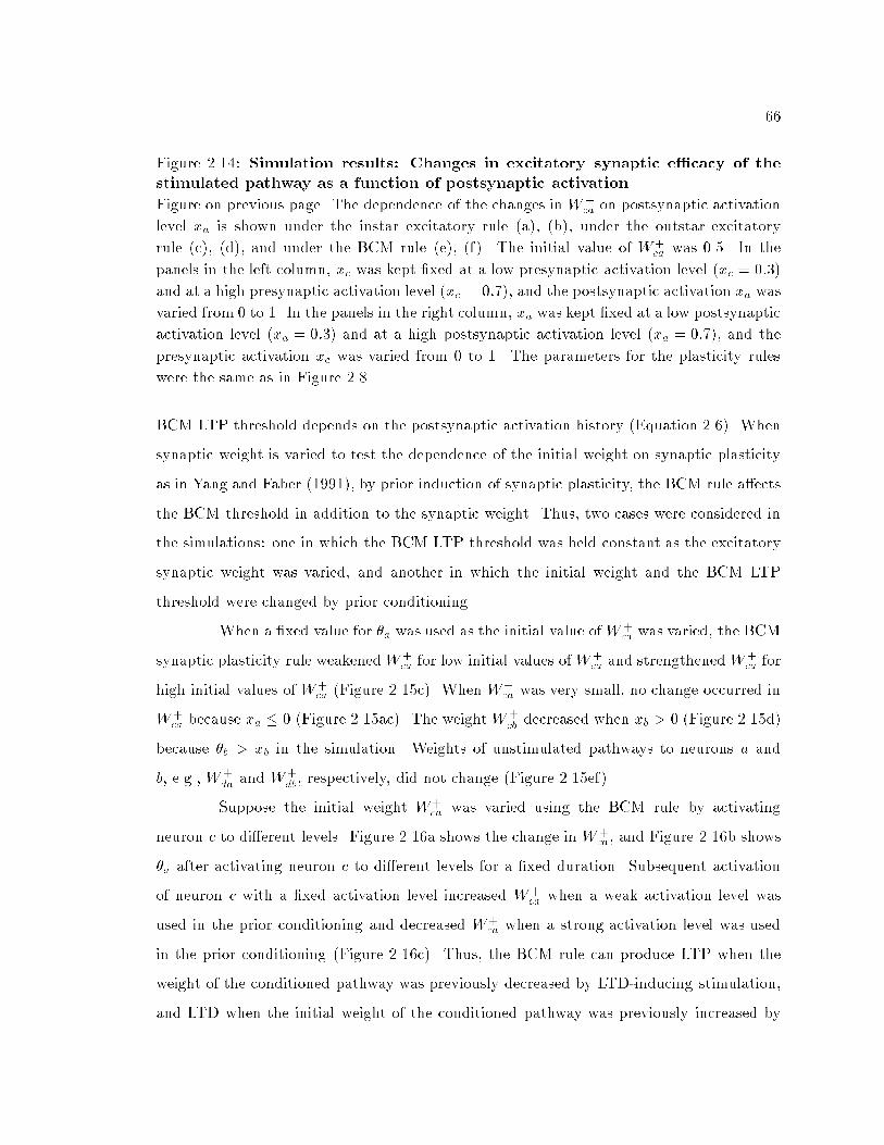
66Figure 2.14: Simulation results: Changes in excitatory synaptic e�cacy of thestimulated pathway as a function of postsynaptic activation.Figure on previous page. The dependence of the changes in W+ca on postsynaptic activationlevel xa is shown under the instar excitatory rule (a), (b), under the outstar excitatoryrule (c), (d), and under the BCM rule (e), (f). The initial value of W+ca was 0.5. In thepanels in the left column, xc was kept �xed at a low presynaptic activation level (xc = 0:3)and at a high presynaptic activation level (xc = 0:7), and the postsynaptic activation xa wasvaried from 0 to 1. In the panels in the right column, xa was kept �xed at a low postsynapticactivation level (xa = 0:3) and at a high postsynaptic activation level (xa = 0:7), and thepresynaptic activation xc was varied from 0 to 1. The parameters for the plasticity ruleswere the same as in Figure 2.8.BCM LTP threshold depends on the postsynaptic activation history (Equation 2.6). Whensynaptic weight is varied to test the dependence of the initial weight on synaptic plasticityas in Yang and Faber (1991), by prior induction of synaptic plasticity, the BCM rule a�ectsthe BCM threshold in addition to the synaptic weight. Thus, two cases were considered inthe simulations: one in which the BCM LTP threshold was held constant as the excitatorysynaptic weight was varied, and another in which the initial weight and the BCM LTPthreshold were changed by prior conditioning.When a �xed value for �a was used as the initial value ofW+ca was varied, the BCMsynaptic plasticity rule weakenedW+ca for low initial values ofW+ca and strengthened W+ca forhigh initial values of W+ca (Figure 2.15c). When W+ca was very small, no change occurred inW+ca because xa � 0 (Figure 2.15ac). The weight W+cb decreased when xb > 0 (Figure 2.15d)because �b > xb in the simulation. Weights of unstimulated pathways to neurons a andb, e.g., W+da and W+db, respectively, did not change (Figure 2.15ef).Suppose the initial weight W+ca was varied using the BCM rule by activatingneuron c to di�erent levels. Figure 2.16a shows the change in W+ca, and Figure 2.16b shows�a after activating neuron c to di�erent levels for a �xed duration. Subsequent activationof neuron c with a �xed activation level increased W+ca when a weak activation level wasused in the prior conditioning and decreased W+ca when a strong activation level was usedin the prior conditioning (Figure 2.16c). Thus, the BCM rule can produce LTP when theweight of the conditioned pathway was previously decreased by LTD-inducing stimulation,and LTD when the initial weight of the conditioned pathway was previously increased by

670.0 0.2 0.4 0.6 0.8 1.0

-0.20

0.00

0.20

0.40

0.60

0.80

1.00

Initial excitatory synaptic weight(a)

Act

ivat

ion

Neuron a

0.0 0.2 0.4 0.6 0.8 1.0-0.20

0.00

0.20

0.40

0.60

0.80

1.00

Initial excitatory synaptic weight(b)

Act

ivat

ion

Neuron b

0.0 0.2 0.4 0.6 0.8 1.0-0.25

-0.20

-0.15

-0.10

-0.05

0.00

0.05

0.10

Initial excitatory synaptic weight(c)

Syn

aptic

pla

stic

ity (

x 0.

1)

Instar excitatory

0.0 0.2 0.4 0.6 0.8 1.0-0.25

-0.20

-0.15

-0.10

-0.05

0.00

0.05

0.10

Initial excitatory synaptic weight(e)

Syn

aptic

pla

stic

ity (

x 0.

1)

Instar excitatory

0.0 0.2 0.4 0.6 0.8 1.0-0.25

-0.20

-0.15

-0.10

-0.05

0.00

0.05

0.10

Initial excitatory synaptic weight(d)

Syn

aptic

pla

stic

ity (

x 0.

1)

Instar excitatory

0.0 0.2 0.4 0.6 0.8 1.0-0.25

-0.20

-0.15

-0.10

-0.05

0.00

0.05

0.10

Initial excitatory synaptic weight(f)

Syn

aptic

pla

stic

ity (

x 0.

1)

Instar excitatory

0.0 0.2 0.4 0.6 0.8 1.0-0.25

-0.20

-0.15

-0.10

-0.05

0.00

0.05

0.10

Initial excitatory synaptic weight(c)

Syn

aptic

pla

stic

ity (

x 0.

1)

Outstar excitatory

0.0 0.2 0.4 0.6 0.8 1.0-0.25

-0.20

-0.15

-0.10

-0.05

0.00

0.05

0.10

Initial excitatory synaptic weight(e)

Syn

aptic

pla

stic

ity (

x 0.

1)

Outstar excitatory

0.0 0.2 0.4 0.6 0.8 1.0-0.25

-0.20

-0.15

-0.10

-0.05

0.00

0.05

0.10

Initial excitatory synaptic weight(d)

Syn

aptic

pla

stic

ity (

x 0.

1)

Outstar excitatory

0.0 0.2 0.4 0.6 0.8 1.0-0.25

-0.20

-0.15

-0.10

-0.05

0.00

0.05

0.10

Initial excitatory synaptic weight(f)

Syn

aptic

pla

stic

ity (

x 0.

1)

Outstar excitatory

0.0 0.2 0.4 0.6 0.8 1.0-0.25

-0.20

-0.15

-0.10

-0.05

0.00

0.05

0.10

Initial excitatory synaptic weight(c)

Syn

aptic

pla

stic

ity (

x 0.

1)

BCM

0.0 0.2 0.4 0.6 0.8 1.0-0.25

-0.20

-0.15

-0.10

-0.05

0.00

0.05

0.10

Initial excitatory synaptic weight(e)

Syn

aptic

pla

stic

ity (

x 0.

1)

BCM

0.0 0.2 0.4 0.6 0.8 1.0-0.25

-0.20

-0.15

-0.10

-0.05

0.00

0.05

0.10

Initial excitatory synaptic weight(d)

Syn

aptic

pla

stic

ity (

x 0.

1)BCM

0.0 0.2 0.4 0.6 0.8 1.0-0.25

-0.20

-0.15

-0.10

-0.05

0.00

0.05

0.10

Initial excitatory synaptic weight(f)

Syn

aptic

pla

stic

ity (

x 0.

1)

BCM

Figure 2.15: Legend on next page.

68Figure 2.15: Simulation results: Changes in excitatory synaptic e�cacy of thestimulated pathway as a function of initial synaptic e�cacy.Figure on previous page. The parameters for the plasticity rules and the activation equationwere the same as in Figure 2.8. The initial network synaptic weights were the same exceptthat W+ca was varied from 0 to 1, and neuron c was activated at a �xed level of 0.5.(a,b) Activation level of neurons a and b, respectively, as W+ca was varied. (c,d) Synapticplasticity in the stimulated pathways from neuron c to neuron a and from neuron c toneuron b, respectively. (e,f) Synaptic plasticity in the unstimulated pathways from neuron dto neuron a and from neuron d to neuron b, asW+ca was varied. For the BCM rule the initialLTP threshold of neurons a and b was �xed at 0.7 asW+ca was varied. There was no synapticweight change according to the instar rule when postsynaptic activation was suppressed(c,d,e,f). Synaptic plasticity was blocked according to the BCM rule when postsynapticactivation was suppressed (c), (d) and when presynaptic stimulation was absent (e), (f).Absence of presynaptic stimulation blocked synaptic plasticity in (e), (f) according to theoutstar rule.LTP-inducing stimulation.Associative synaptic plasticityAssociative LTP (Brown et al., 1990; Levy & Steward, 1979; Barrionuevo &Brown, 1983; Kelso & Brown, 1986) refers to LTP produced in a weak excitatory pathwayto a neuron by simultaneous stimulation of the weak excitatory pathway and a strongexcitatory pathway to the neuron; but LTP is not induced in the weak excitatory pathwayto the neuron by exclusive stimulation of the weak or the strong excitatory pathway.Figures 2.18 and 2.20 show changes in the synaptic e�cacy governed by the three rules inresponse to stimulation of independent excitatory pathways to neuron a. In the simulations,the excitatory pathway from neuron e to neuron a in Figure 2.7 was weak, and the excitatorypathway from neuron c to neuron a in Figure 2.7 was strong.In the simulations in Figures 2.17 and 2.18, when the weak excitatory pathwayfrom neuron e to neuron a was stimulated, neuron a was inactive (Figure 2.17a). Therefore,W+ea and W+ca did not change according to the instar and the BCM excitatory synapticplasticity rules (Figure 2.18ab) because postsynaptic activation was below zero. The outstarexcitatory synaptic plasticity rules weakened W+ea because W+ea was greater than Q(xa) = 0(Figure 2.18a);W+ca did not change because the pathway from neuron c to neuron a was not

690.0 0.2 0.4 0.6 0.8 1.0

-0.02

0.00

0.02

0.04

0.06

0.08

0.10

0.12

Presynaptic stimulation strength(a)

Syn

aptic

pla

stic

ity

Synaptic plasticity in pathway ca

0.0 0.2 0.4 0.6 0.8 1.00.00

0.20

0.40

0.60

0.80

Presynaptic stimulation strength(b)

Act

ivat

ion

or B

CM

LT

P th

resh

old

Activation level of neuron a

0.0 0.2 0.4 0.6 0.8 1.00.00

0.20

0.40

0.60

0.80

Presynaptic stimulation strength(b)

Act

ivat

ion

or B

CM

LT

P th

resh

old LTP threshold of neuron a

0.0 0.2 0.4 0.6 0.8 1.0-0.10

0.00

0.10

0.20

0.30

Presynaptic stimulation strength(c)

Syn

aptic

pla

stic

ity (

x 0.

01) Synaptic plasticity in pathway ca

Figure 2.16: Legend on next page.

70Figure 2.16: Simulation results: Changes in excitatory synaptic e�cacy of thestimulated pathway according to the BCM rule as a function of prior presynapticstimulation.Figure on previous page. The initial network synaptic weights, the BCM rule parameters,and the activation equation parameters are the same as in Figure 2.8. The initial LTPthreshold of neurons a and b was 0.7. (a) The change in W+ca after stimulating neuron c atdi�erent activation levels for 20 iterations. The LTP threshold was changed according to theequation in Figure 2.12. The LTP threshold of neuron a and the activation level of neuron ain response to activation of neuron c at xc = 0:3 are shown following the stimulation ofneuron c for 20 iterations (b). The changes in W+ca when neuron c was activated at xc = 0:3are also shown in (c).stimulated. Thus, according to the three excitatory synaptic plasticity rules, stimulation ofa weak excitatory pathway to a neuron may not induce LTP in the weak pathway, becausenetwork interaction may render the neuron inactive.When the strong excitatory pathway from neuron c to neuron a was stimulated,neuron a became strongly activated (Figure 2.17a). The instar excitatory synaptic plasticityrule weakened W+ea because xe = 0 (Figure 2.18c). The outstar and the BCM excitatorysynaptic plasticity rules did not modify W+ea because xe = 0 (Figure 2.18c). All three rulesproduced LTP in the stimulated strong excitatory pathway from neuron c to neuron a whenxc was large (Figure 2.18d). Thus, stimulation of the strong excitatory pathway alone didnot produce LTP in the weak pathway.When neurons c and e were simultaneously activated at the same level, xa wassmaller than when xc was stimulated alone (Figure 2.17a); the strong lateral inhibitoryinteractions between neurons a and b reduced their activation levels. In this particularnetwork, when neurons c and e were simultaneously stimulated with the same strength, theinstar excitatory synaptic plasticity rule produced LTP in W+ea and W+ca at high stimulationstrengths (Figure 2.18ef). Thus, in this network the instar excitatory synaptic plasticityrule exhibited associative LTP when the presynaptic stimulation strength was high. Whenneurons c and e were simultaneously stimulated with the same stimulation strength, theyhad di�erent LTP thresholds under the instar rule (Figure 2.18ef). When the outstarrule was used during simultaneous stimulation of neurons c and e, LTP was produced inW+ea at high stimulation strengths (Figure 2.18e), but W+ca underwent LTD even at high

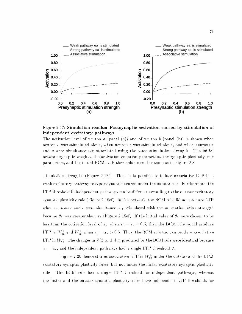
710.0 0.2 0.4 0.6 0.8 1.0

-0.20

0.00

0.20

0.40

0.60

0.80

1.00

Presynaptic stimulation strength(a)

Act

ivat

ion

Weak pathway is stimulatedea

0.0 0.2 0.4 0.6 0.8 1.0-0.20

0.00

0.20

0.40

0.60

0.80

1.00

Presynaptic stimulation strength(a)

Act

ivat

ion

Strong pathway is stimulatedca

0.0 0.2 0.4 0.6 0.8 1.0-0.20

0.00

0.20

0.40

0.60

0.80

1.00

Presynaptic stimulation strength(a)

Act

ivat

ion

Associative stimulation

0.0 0.2 0.4 0.6 0.8 1.0-0.20

0.00

0.20

0.40

0.60

0.80

1.00

Presynaptic stimulation strength(b)

Act

ivat

ion

Weak pathway is stimulatedea

0.0 0.2 0.4 0.6 0.8 1.0-0.20

0.00

0.20

0.40

0.60

0.80

1.00

Presynaptic stimulation strength(b)

Act

ivat

ion

Strong pathway is stimulatedca

0.0 0.2 0.4 0.6 0.8 1.0-0.20

0.00

0.20

0.40

0.60

0.80

1.00

Presynaptic stimulation strength(b)

Act

ivat

ion

Associative stimulation

Figure 2.17: Simulation results: Postsynaptic activation caused by stimulation ofindependent excitatory pathways.The activation level of neuron a (panel (a)) and of neuron b (panel (b)) is shown whenneuron e was stimulated alone, when neuron c was stimulated alone, and when neurons eand c were simultaneously stimulated using the same stimulation strength. The initialnetwork synaptic weights, the activation equation parameters, the synaptic plasticity ruleparameters, and the initial BCM LTP thresholds were the same as in Figure 2.8.stimulation strengths (Figure 2.18f). Thus, it is possible to induce associative LTP in aweak excitatory pathway to a postsynaptic neuron under the outstar rule. Furthermore, theLTP threshold in independent pathways can be di�erent according to the outstar excitatorysynaptic plasticity rule (Figure 2.18ef). In this network, the BCM rule did not produce LTPwhen neurons c and e were simultaneously stimulated with the same stimulation strengthbecause �a was greater than xa (Figure 2.18ef). If the initial value of �a were chosen to beless than the activation level of xa when xc = xe = 0:5, then the BCM rule would produceLTP in W+ea and W+ca when xc = xe > 0:5. Thus, the BCM rule too can produce associativeLTP inW+ea. The changes in W+ea andW+ca produced by the BCM rule were identical becausexc = xe, and the independent pathways had a single LTP threshold �a.Figure 2.20 demonstrates associative LTP in W+ea under the outstar and the BCMexcitatory synaptic plasticity rules, but not under the instar excitatory synaptic plasticityrule. The BCM rule has a single LTP threshold for independent pathways, whereasthe instar and the outstar synaptic plasticity rules have independent LTP thresholds for

720.0 0.2 0.4 0.6 0.8 1.0

-0.20

-0.10

0.00

0.10

0.20

Presynaptic stimulation strength(a)

Syn

aptic

pla

stic

ity (

x 0.

1)Instar excitatory

0.0 0.2 0.4 0.6 0.8 1.0-0.20

-0.10

0.00

0.10

0.20

Presynaptic stimulation strength(b)

Syn

aptic

pla

stic

ity (

x 0.

1)

Instar excitatory

0.0 0.2 0.4 0.6 0.8 1.0-0.20

-0.10

0.00

0.10

0.20

Presynaptic stimulation strength(c)

Syn

aptic

pla

stic

ity (

x 0.

1)

Instar excitatory

0.0 0.2 0.4 0.6 0.8 1.0-0.20

-0.10

0.00

0.10

0.20

Presynaptic stimulation strength(d)

Syn

aptic

pla

stic

ity (

x 0.

1)

Instar excitatory

0.0 0.2 0.4 0.6 0.8 1.0-0.20

-0.10

0.00

0.10

0.20

Presynaptic stimulation strength(e)

Syn

aptic

pla

stic

ity (

x 0.

1)

Instar excitatory

0.0 0.2 0.4 0.6 0.8 1.0-0.20

-0.10

0.00

0.10

0.20

Presynaptic stimulation strength(f)

Syn

aptic

pla

stic

ity (

x 0.

1)

Instar excitatory

0.0 0.2 0.4 0.6 0.8 1.0-0.20

-0.10

0.00

0.10

0.20

Presynaptic stimulation strength(a)

Syn

aptic

pla

stic

ity (

x 0.

1)Outstar excitatory

0.0 0.2 0.4 0.6 0.8 1.0-0.20

-0.10

0.00

0.10

0.20

Presynaptic stimulation strength(b)

Syn

aptic

pla

stic

ity (

x 0.

1)

Outstar excitatory

0.0 0.2 0.4 0.6 0.8 1.0-0.20

-0.10

0.00

0.10

0.20

Presynaptic stimulation strength(c)

Syn

aptic

pla

stic

ity (

x 0.

1)

Outstar excitatory

0.0 0.2 0.4 0.6 0.8 1.0-0.20

-0.10

0.00

0.10

0.20

Presynaptic stimulation strength(d)

Syn

aptic

pla

stic

ity (

x 0.

1)

Outstar excitatory

0.0 0.2 0.4 0.6 0.8 1.0-0.20

-0.10

0.00

0.10

0.20

Presynaptic stimulation strength(e)

Syn

aptic

pla

stic

ity (

x 0.

1)

Outstar excitatory

0.0 0.2 0.4 0.6 0.8 1.0-0.20

-0.10

0.00

0.10

0.20

Presynaptic stimulation strength(f)

Syn

aptic

pla

stic

ity (

x 0.

1)

Outstar excitatory

0.0 0.2 0.4 0.6 0.8 1.0-0.20

-0.10

0.00

0.10

0.20

Presynaptic stimulation strength(a)

Syn

aptic

pla

stic

ity (

x 0.

1)

BCM

0.0 0.2 0.4 0.6 0.8 1.0-0.20

-0.10

0.00

0.10

0.20

Presynaptic stimulation strength(b)

Syn

aptic

pla

stic

ity (

x 0.

1)

BCM

0.0 0.2 0.4 0.6 0.8 1.0-0.20

-0.10

0.00

0.10

0.20

Presynaptic stimulation strength(c)

Syn

aptic

pla

stic

ity (

x 0.

1)

BCM

0.0 0.2 0.4 0.6 0.8 1.0-0.20

-0.10

0.00

0.10

0.20

Presynaptic stimulation strength(d)

Syn

aptic

pla

stic

ity (

x 0.

1)BCM

0.0 0.2 0.4 0.6 0.8 1.0-0.20

-0.10

0.00

0.10

0.20

Presynaptic stimulation strength(e)

Syn

aptic

pla

stic

ity (

x 0.

1)

BCM

0.0 0.2 0.4 0.6 0.8 1.0-0.20

-0.10

0.00

0.10

0.20

Presynaptic stimulation strength(f)

Syn

aptic

pla

stic

ity (

x 0.

1)

BCM

Figure 2.18: Legend on next page.

73Figure 2.18: Simulation results: Associative synaptic plasticity.Figure on previous page. The simulation parameters are given in Figure 2.17. The panels inthe left column show changes in the weak pathway from neuron e to neuron a, and the panelsin the right column show changes in the strong pathway from neuron c to neuron a, whenthe weak pathway alone was stimulated (top row), the strong pathway alone was stimulated(middle row), and the weak and the strong pathways were simultaneously stimulated usingthe same stimulation strength (bottom row). Activation of neuron a was suppressed whenthe pathway ea was stimulated, and therefore the weight of pathway ea and pathway ca wasnot changed under the instar rule and the BCM rule (a), (b). The weight of pathway ca wasnot changed under the outstar rule (b), since the pathway was not stimulated. (c) Synapticplasticity in pathway ea was blocked according to the outstar rule and the BCM rule becausepathway ea was not stimulated.0.0 0.2 0.4 0.6 0.8 1.0

-0.20

0.00

0.20

0.40

0.60

0.80

1.00

Presynaptic stimulation strength(a)

Act

ivat

ion

Weak pathway is stimulatedea

0.0 0.2 0.4 0.6 0.8 1.0-0.20

0.00

0.20

0.40

0.60

0.80

1.00

Presynaptic stimulation strength(a)

Act

ivat

ion

Strong pathway is stimulatedca

0.0 0.2 0.4 0.6 0.8 1.0-0.20

0.00

0.20

0.40

0.60

0.80

1.00

Presynaptic stimulation strength(a)

Act

ivat

ion

Associative stimulation

0.0 0.2 0.4 0.6 0.8 1.0-0.20

0.00

0.20

0.40

0.60

0.80

1.00

Presynaptic stimulation strength(b)

Act

ivat

ion

Weak pathway is stimulatedea

0.0 0.2 0.4 0.6 0.8 1.0-0.20

0.00

0.20

0.40

0.60

0.80

1.00

Presynaptic stimulation strength(b)

Act

ivat

ion

Strong pathway is stimulatedca

0.0 0.2 0.4 0.6 0.8 1.0-0.20

0.00

0.20

0.40

0.60

0.80

1.00

Presynaptic stimulation strength(b)

Act

ivat

ion

Associative stimulation

Figure 2.19: Simulation results: Postsynaptic activation caused by stimulationof independent excitatory pathways in a network with asymmetric lateralinhibitory weights.The activation of neuron a (panel (a)) and of neuron b (panel (b)) is shown when neuron ewas stimulated alone, when neuron c was stimulated alone, and when neurons e and c weresimultaneously stimulated using the same stimulation strength. The activation equationparameters, the synaptic plasticity rule parameters, and the initial BCM LTP thresholdswere the same as in Figure 2.8. The initial network synaptic weights were the same as inFigure 2.8 except that W�ab = 0:4 and W�ba = 0:1.

740.0 0.2 0.4 0.6 0.8 1.0

-0.20

-0.10

0.00

0.10

0.20

0.30

Presynaptic stimulation strength(a)

Syn

aptic

pla

stic

ity (

x 0.

1)Instar excitatory

0.0 0.2 0.4 0.6 0.8 1.0-0.20

-0.10

0.00

0.10

0.20

0.30

Presynaptic stimulation strength(b)

Syn

aptic

pla

stic

ity (

x 0.

1)

Instar excitatory

0.0 0.2 0.4 0.6 0.8 1.0-0.20

-0.10

0.00

0.10

0.20

0.30

Presynaptic stimulation strength(c)

Syn

aptic

pla

stic

ity (

x 0.

1)

Instar excitatory

0.0 0.2 0.4 0.6 0.8 1.0-0.20

-0.10

0.00

0.10

0.20

0.30

Presynaptic stimulation strength(d)

Syn

aptic

pla

stic

ity (

x 0.

1)

Instar excitatory

0.0 0.2 0.4 0.6 0.8 1.0-0.20

-0.10

0.00

0.10

0.20

0.30

Presynaptic stimulation strength(e)

Syn

aptic

pla

stic

ity (

x 0.

1)

Instar excitatory

0.0 0.2 0.4 0.6 0.8 1.0-0.20

-0.10

0.00

0.10

0.20

0.30

Presynaptic stimulation strength(f)

Syn

aptic

pla

stic

ity (

x 0.

1)

Instar excitatory

0.0 0.2 0.4 0.6 0.8 1.0-0.20

-0.10

0.00

0.10

0.20

0.30

Presynaptic stimulation strength(a)

Syn

aptic

pla

stic

ity (

x 0.

1)Outstar excitatory

0.0 0.2 0.4 0.6 0.8 1.0-0.20

-0.10

0.00

0.10

0.20

0.30

Presynaptic stimulation strength(b)

Syn

aptic

pla

stic

ity (

x 0.

1)

Outstar excitatory

0.0 0.2 0.4 0.6 0.8 1.0-0.20

-0.10

0.00

0.10

0.20

0.30

Presynaptic stimulation strength(c)

Syn

aptic

pla

stic

ity (

x 0.

1)

Outstar excitatory

0.0 0.2 0.4 0.6 0.8 1.0-0.20

-0.10

0.00

0.10

0.20

0.30

Presynaptic stimulation strength(d)

Syn

aptic

pla

stic

ity (

x 0.

1)

Outstar excitatory

0.0 0.2 0.4 0.6 0.8 1.0-0.20

-0.10

0.00

0.10

0.20

0.30

Presynaptic stimulation strength(e)

Syn

aptic

pla

stic

ity (

x 0.

1)

Outstar excitatory

0.0 0.2 0.4 0.6 0.8 1.0-0.20

-0.10

0.00

0.10

0.20

0.30

Presynaptic stimulation strength(f)

Syn

aptic

pla

stic

ity (

x 0.

1)

Outstar excitatory

0.0 0.2 0.4 0.6 0.8 1.0-0.20

-0.10

0.00

0.10

0.20

0.30

Presynaptic stimulation strength(a)

Syn

aptic

pla

stic

ity (

x 0.

1)

BCM

0.0 0.2 0.4 0.6 0.8 1.0-0.20

-0.10

0.00

0.10

0.20

0.30

Presynaptic stimulation strength(b)

Syn

aptic

pla

stic

ity (

x 0.

1)

BCM

0.0 0.2 0.4 0.6 0.8 1.0-0.20

-0.10

0.00

0.10

0.20

0.30

Presynaptic stimulation strength(c)

Syn

aptic

pla

stic

ity (

x 0.

1)

BCM

0.0 0.2 0.4 0.6 0.8 1.0-0.20

-0.10

0.00

0.10

0.20

0.30

Presynaptic stimulation strength(d)

Syn

aptic

pla

stic

ity (

x 0.

1)BCM

0.0 0.2 0.4 0.6 0.8 1.0-0.20

-0.10

0.00

0.10

0.20

0.30

Presynaptic stimulation strength(e)

Syn

aptic

pla

stic

ity (

x 0.

1)

BCM

0.0 0.2 0.4 0.6 0.8 1.0-0.20

-0.10

0.00

0.10

0.20

0.30

Presynaptic stimulation strength(f)

Syn

aptic

pla

stic

ity (

x 0.

1)

BCM

Figure 2.20: Legend on next page.

75Figure 2.20: Simulation results: Associative synaptic plasticity in a network withasymmetric lateral inhibitory weights.Figure on previous page. The simulation parameters are given in Figure 2.19. SeeFigure 2.18 for conventions. The weights of pathways ca and ea were not changed underthe outstar rule and the BCM rule (b), (c) because the pathways were not stimulated.independent pathways (Figure 2.20ef).In the case of the outstar and the BCM excitatory synaptic plasticity rules, todemonstrate associative plasticity the postsynaptic activation level should be below the LTPthreshold of the weak pathway when the weak pathway is stimulated alone. However, whenthe weak and a strong pathway are simultaneously stimulated, the postsynaptic activationshould exceed the LTP threshold of the weak pathway. Under the outstar and the BCMexcitatory synaptic plasticity rules, no synaptic plasticity occurs in the unstimulated weakpathway when the strong pathway alone is stimulated. In the case of the instar excitatorysynaptic plasticity rule, to produce associative plasticity the postsynaptic activation shouldbe suppressed when the weak pathway is stimulated alone, but when the weak and thestrong pathway are simultaneously stimulated the postsynaptic neuron should be activated.If stimulation of the weak pathway activates the postsynaptic neuron, thenassociative LTP cannot be produced according to the instar rule alone. When thepostsynaptic neuron is active, then the sign of weight change depends only on thepresynaptic stimulation strength to the weak pathway and the synaptic strength of theweak pathway. Any stimulation that produces LTP (LTD) in the weak pathway when theweak pathway alone is stimulated will produce LTP (LTD) in the weak pathway whenthe weak pathway and the strong pathway are simultaneously stimulated with the samestimulation strength.2.3.4 Combined e�ects of instar and outstar excitatory synaptic plasticityrulesArtola et al. (1990) found that for a �xed presynaptic stimulation at thewhite matter{layer 6 border, synaptic plasticity in the excitatory pathways tolayers 2{4 neurons depended on the postsynaptic activation level. Plasticity was blocked,

76or very little LTD was produced, when the postsynaptic activation was suppressed belowa threshold. Increasing postsynaptic activation above the threshold produced larger LTD;and further increase in postsynaptic activation above a second higher threshold producedLTP. In this section, it is shown that a combination of the instar and the outstar rulesmodels the results of Artola et al. (1990).Stimulation at the white matter{layer 6 border can activate geniculocorticalpathways and corticocortical pathways to neurons in layers 2{4 (Kirkwood et al., 1993).In the absence of any pharmacological treatment, white matter stimulation producescomplex postsynaptic potentials involving monosynaptic and polysynaptic EPSP and IPSPsequences (Fr�egnac et al., 1994). A measure of synaptic e�cacy such as the amplitude of theearly peak of the postsynaptic potential may involve interactions of a variety of membranecurrents, and therefore, this measure of synaptic e�cacy of the pathway from white matteris an estimate of the \e�ective weight" of the pathway (Fr�egnac et al., 1994).In the simulations presented in this section, it was assumed that plasticity ina�erent feedforward (Felleman & Van Essen, 1991; Maunsell & Van Essen, 1983) excitatorypathways from lateral geniculate nucleus to neurons in layers 2{4 is governed by the instarexcitatory rule and that plasticity in feedback (Felleman & Van Essen, 1991; Maunsell &Van Essen, 1983) excitatory corticocortical pathways to neurons in layers 2{4 is governedby the outstar excitatory rule. In Sections 2.4.3 and 2.4.4, a plausible computational basisfor the above assumptions is discussed.Figure 2.21 shows the e�ects of combining the weights of feedforward and feedbackpathways. In Figure 2.21, a postsynaptic neuron k was innervated by a feedforwardpathway ik with synaptic weight W+ik , and by a feedback pathway jk with synaptic weightW+jk. The feedforward pathway synaptic plasticity was governed by the instar excitatoryrule, and the feedback pathway synaptic plasticity was governed by the outstar excitatoryrule. In the simulation, both the pathways were stimulated using the same stimulation.Because the total excitation to the postsynaptic neuron was given by Equation 2.2, which islinear in the synaptic weights, and because the presynaptic stimulation strength to the twopathways was the same, the e�ective weight of the two pathways was computed by addingtheir synaptic weights.

770.0 0.2 0.4 0.6 0.8 1.0

-0.60

-0.30

0.00

0.30

0.60

0.90

1.20

Postsynaptic activation(a)

Syn

aptic

pla

stic

ityInstar excitatory

0.0 0.2 0.4 0.6 0.8 1.0-0.60

-0.30

0.00

0.30

0.60

0.90

1.20

Postsynaptic activation(a)

Syn

aptic

pla

stic

ityOutstar excitatory

0.0 0.2 0.4 0.6 0.8 1.0-0.60

-0.30

0.00

0.30

0.60

0.90

1.20

Postsynaptic activation(a)

Syn

aptic

pla

stic

ity

Instar + outstar excitatory

0.0 0.2 0.4 0.6 0.8 1.0-0.60

-0.30

0.00

0.30

0.60

0.90

1.20

Postsynaptic activation(b)

Syn

aptic

pla

stic

ity

Instar excitatory

0.0 0.2 0.4 0.6 0.8 1.0-0.60

-0.30

0.00

0.30

0.60

0.90

1.20

Postsynaptic activation(b)

Syn

aptic

pla

stic

ity

Outstar excitatory

0.0 0.2 0.4 0.6 0.8 1.0-0.60

-0.30

0.00

0.30

0.60

0.90

1.20

Postsynaptic activation(b)

Syn

aptic

pla

stic

ity

Instar + outstar excitatory

0.0 0.2 0.4 0.6 0.8 1.0-0.60

-0.30

0.00

0.30

0.60

0.90

1.20

Postsynaptic activation(c)

Syn

aptic

pla

stic

ity

Instar excitatory

0.0 0.2 0.4 0.6 0.8 1.0-0.60

-0.30

0.00

0.30

0.60

0.90

1.20

Postsynaptic activation(c)

Syn

aptic

pla

stic

ity

Outstar excitatory

0.0 0.2 0.4 0.6 0.8 1.0-0.60

-0.30

0.00

0.30

0.60

0.90

1.20

Postsynaptic activation(c)

Syn

aptic

pla

stic

ity

Instar + outstar excitatory

0.0 0.2 0.4 0.6 0.8 1.0-0.60

-0.30

0.00

0.30

0.60

0.90

1.20

Postsynaptic activation(d)

Syn

aptic

pla

stic

ity

Instar excitatory

0.0 0.2 0.4 0.6 0.8 1.0-0.60

-0.30

0.00

0.30

0.60

0.90

1.20

Postsynaptic activation(d)

Syn

aptic

pla

stic

ity

Outstar excitatory

0.0 0.2 0.4 0.6 0.8 1.0-0.60

-0.30

0.00

0.30

0.60

0.90

1.20

Postsynaptic activation(d)

Syn

aptic

pla

stic

ityInstar + outstar excitatory

0.0 0.2 0.4 0.6 0.8 1.0-0.60

-0.30

0.00

0.30

0.60

0.90

1.20

Postsynaptic activation(e)

Syn

aptic

pla

stic

ity

Instar excitatory

0.0 0.2 0.4 0.6 0.8 1.0-0.60

-0.30

0.00

0.30

0.60

0.90

1.20

Postsynaptic activation(e)

Syn

aptic

pla

stic

ity

Outstar excitatory

0.0 0.2 0.4 0.6 0.8 1.0-0.60

-0.30

0.00

0.30

0.60

0.90

1.20

Postsynaptic activation(e)

Syn

aptic

pla

stic

ity

Instar + outstar excitatory

0.0 0.2 0.4 0.6 0.8 1.0-0.60

-0.30

0.00

0.30

0.60

0.90

1.20

Postsynaptic activation(f)

Syn

aptic

pla

stic

ity

Instar excitatory

0.0 0.2 0.4 0.6 0.8 1.0-0.60

-0.30

0.00

0.30

0.60

0.90

1.20

Postsynaptic activation(f)

Syn

aptic

pla

stic

ity

Outstar excitatory

0.0 0.2 0.4 0.6 0.8 1.0-0.60

-0.30

0.00

0.30

0.60

0.90

1.20

Postsynaptic activation(f)

Syn

aptic

pla

stic

ity

Instar + outstar excitatory

Figure 2.21: Legend on next page.

78Figure 2.21: Simulation results: Synaptic plasticity with �xed presynapticstimulation and variable postsynaptic activation level under the instar and theoutstar excitatory synaptic plasticity rules.Figure on previous page. In this simulation, a postsynaptic neuron received feedforwardand feedback pathways. The feedforward pathway synaptic plasticity was governed bythe instar excitatory rule, and the feedback pathway synaptic plasticity was governed bythe outstar excitatory rule. The two pathways were stimulated by the same stimulationstrength, and the e�ective synaptic weight of the two pathways was obtained by addingthe synaptic weights of the two pathways. The presynaptic stimulation strength of thetwo pathways was held constant, and the postsynaptic activation was varied. (a){(e) Thesynaptic weight changes were computed after pairing the pre- and postsynaptic activationfor 20 iteration. (f) The synaptic weight changes were computed after a single pairing of thepre- and postsynaptic activation. The initial synaptic weight of the feedforward pathwaywas 0.5, and the initial synaptic weight of the feedback pathway was 0.05. The presynapticstimulation strength was 0.1 in panels (a) and (f), 0.4 in panel (b), and 0.6 in panel (c).In panels (d) and (e), the initial synaptic weight of the feedforward pathway was 0.5, andthe initial synaptic weight of the feedback pathway was 0.45. The presynaptic stimulationstrength was 0.1 in panel (d) and 0.4 in panel (e). The parameters for the instar and theoutstar rules were the same as in Figure 2.8.The changes in the combined synaptic weight according to the instar andthe outstar excitatory synaptic plasticity rules in Figure 2.21a are similar to thoseexperimentally observed by Artola et al. (1990). However, the changes in the combinedweight of the feedforward and the feedback pathways produced by the instar and the outstarexcitatory synaptic plasticity rules were parameter dependent.The following paragraphs analyze the parameter dependence of the combinedweight changes based on the combination of the instar and the outstar excitatory synapticplasticity rules. The shape of the curve relating the combined weight changes andpostsynaptic activation level depends on the duration of stimulation, the presynapticstimulation strength, and the initial synaptic weights.In Figure 2.21a the presynaptic stimulation was presented for 20 time steps.Under the instar excitatory rule, the feedforward weight change reached an asymptotebecause presynaptic stimulation was �xed while postsynaptic activation was varied. Theoutstar excitatory rule caused the feedforward pathway weight to approach the postsynapticactivation level, and the weight change in the feedback pathway did not reach an asymptote

79as the postsynaptic activation was increased. Thus, as the postsynaptic activation level wasincreased, the feedforward pathway weight change equilibrated, but the feedback pathwayweight change increased, and the change in combined weight of the two pathways went fromLTD to LTP (Figure 2.21a). When the postsynaptic activation was less than or equal tozero, the plasticity under the instar rule was disabled, but the plasticity in the outstar rule,which is enabled by presynaptic stimulation alone, caused a small LTD in the feedbackpathway because the initial weight of the feedback pathway was small.In Figures 2.21b and 2.21c, the presynaptic stimulation strength was varied.When the presynaptic stimulation strength was close to but less than the feedforwardpathway synaptic weight (Figure 2.21b), the maximal decrease in the feedforward pathwayaccording to the instar rule was small, and therefore the LTP threshold for the combinedsynaptic weight decreased. When the presynaptic stimulation strength was close to butgreater than the feedforward pathway synaptic weight (Figure 2.21c), the feedforwardpathway underwent LTP according to the instar rule, and the LTP threshold for thecombined synaptic weight decreased even further. When the initial synaptic weight ofthe feedback pathway was large, large LTD was produced in the combined synaptic weightwhen the postsynaptic neuron was inactive (Figures 2.21de). In Figure 2.21f, the synapticweight changes are shown after only one iteration when the weights were far from theirequilibrium values. In this case, the combined weight decreased.The instar and the outstar rules alone can not reproduce the experimental results;in fact, the instar and the outstar rules alone cannot produce the results for any parametervalues. If the instar rule alone were used for a �xed presynaptic activation, the sign ofthe synaptic weight change would be �xed as the postsynaptic activation was changed(Figure 2.14). If the outstar rule alone were used for a �xed presynaptic activation, themaximal LTD would be produced when the postsynaptic neuron was hyperpolarized orinactive (Figure 2.14).2.3.5 Characteristics of the outstar inhibitory synaptic plasticity ruleThere have been only a few experiments on lateral inhibitory synaptic plasticity(e.g., Levy & Desmond, 1985; Miles & Wong, 1987; Rutherford et al., 1997).

80Levy and Desmond (1985) suggested several inhibitory synaptic plasticity rules, includingthe outstar inhibitory rule, to model some aspects of classical conditioning. To motivatefurther experimentation on lateral inhibitory synaptic plasticity, predictions of the outstarlateral inhibitory synaptic plasticity rule (Marshall, 1990a, 1995a; Marshall & Gupta, 1998)are presented. As in the case of the excitatory synaptic plasticity rules, changes in thelateral inhibitory synaptic weights under the outstar lateral inhibitory synaptic plasticityrule are studied as a function of input excitation to model neurons, pre- and postsynapticactivation, and initial lateral inhibitory weights.The properties of the outstar lateral inhibitory synaptic plasticity rule areillustrated using the simple neural network described in Section 2.3.3 (Figure 2.7). Inthe simulations in this section, only the lateral inhibitory pathway weights were plastic; theexcitatory pathway weights were held constant.Synaptic plasticity in lateral inhibitory synapses as a function of input excitationFigure 2.22 shows the activation of neurons a and b as xd was varied from 0 to 1.The activations xa and xb increased as xd was increased (Figure 2.22ab), and xa and xbremained equal, because of the symmetry of the initial weights.Synaptic plasticity in the lateral inhibitory pathways between neurons a and b asa function of input stimulation strength is shown in Figure 2.22cd. When the excitatoryinput to neurons a and b was low, both neurons were weakly activated (Figure 2.22ab),and according to the outstar lateral inhibitory plasticity rule pathway the lateral inhibitorypathways between the two neurons underwent LTD, because R(xa) and R(xb) were lessthan W�ba and W�ab, respectively. As xd increased, xa and xb increased (Figure 2.22ab), andW�ba and W�ab were potentiated (Figure 2.22cd).In Figure 2.23, neuron c was stimulated. Figure 2.23ab shows the activation ofneurons a and b as xc was varied from 0 to 1. When xb was below zero, according tothe outstar lateral inhibitory synaptic plasticity rule W�ba did not undergo any change, andW�ab decreased (Figure 2.23cd). At high values of xc, when xa and xb are greater thanzero, changes in the lateral inhibitory pathway weights depended on the initial value of theinhibitory weights and on the postsynaptic activation level (Figure 2.23cd); the inhibitory

810.0 0.2 0.4 0.6 0.8 1.0

-0.20

0.00

0.20

0.40

0.60

0.80

1.00

Presynaptic stimulation strength(a)

Act

ivat

ion

Neuron a

0.0 0.2 0.4 0.6 0.8 1.0-0.20

0.00

0.20

0.40

0.60

0.80

1.00

Presynaptic stimulation strength(b)

Act

ivat

ion

Neuron b

0.0 0.2 0.4 0.6 0.8 1.0-0.010.000.010.020.030.040.050.060.070.080.09

Presynaptic stimulation strength(c)

Syn

aptic

pla

stic

ity (

x 0.

1)

Outstar inhibitory

0.0 0.2 0.4 0.6 0.8 1.0-0.010.000.010.020.030.040.050.060.070.080.09

Presynaptic stimulation strength(d)

Syn

aptic

pla

stic

ity (

x 0.

1)

Outstar inhibitory

Figure 2.22: Simulation results: Changes in inhibitory synaptic e�cacy underthe outstar inhibitory synaptic plasticity rule as a function of input excitation.Figure on previous page. In this simulation, the initial pathway synaptic weights in thenetwork shown in Figure 2.4 were assigned as follows: W+ca = 0:5, W+cb = 0:25, W+da = 0:4,W+db = 0:4, W+ea = 0:25, W+eb = 0:5, W�ab = W�ba = 0:2. The parameters for the activationequation (Equation 2.1) were A = 0:1, B = 1, C = 0:05, � = 1, and = 15. The activationlevel was computed using the Euler method with a time step of 0.04 until t = 40. The initialactivation level of neurons a and b was set to zero. The parameters for the outstar lateralinhibitory synaptic plasticity rule were assigned the following values: � = 0:1, H(x) = [x],and R(x) = 2[x]. The �gure shows the synaptic weight changes according to the outstarlateral inhibitory synaptic plasticity rule after activating neuron d. The activation levelof neuron d, xd, was varied from 0 to 1. Panels (a) and (b) show the activation level ofneurons a and b, respectively, as xd was varied, and panels (c) and (d) show changes in W�aband W�ba, respectively, as xd was varied.

82pathway from the strongly active neuron a to the weakly active neuron b weakened (becameless inhibitory), while the inhibitory pathway from the weakly active neuron b to the stronglyactive neuron a strengthened.Figure 2.24 shows the changes in the lateral inhibitory pathways when a�xed stimulation was continuously applied to neuron c. The lateral inhibitory weightsequilibrated to a value proportional to the postsynaptic activation level (Figure 2.24cd),and the rate of change approached zero as the lateral inhibitory weights approached theirequilibrium values (Figure 2.24ef).Synaptic plasticity in lateral inhibitory synapses as a function of activation levelof the pre- and postsynaptic neuronsIn Figure 2.25a, activation level of postsynaptic neuron b was varied for �xedvalues of activation level of presynaptic neuron a. As xb was increased, the change in W�abwent from LTD to LTP. As xa was increased, the magnitude of change in W�ab increased.In Figure 2.25b, activation level of presynaptic neuron a was varied for �xed values of theactivation level of postsynaptic neuron b. As xa was increased the sign of change in W�abwas �xed, but the magnitude of change increased. As xb was increased, the change in W�abwent from LTD to LTP.Synaptic plasticity in lateral inhibitory synapses as a function of initialinhibitory synaptic e�cacyThe simulations in this section illustrate that under the outstar lateral inhibitorysynaptic plasticity rule, in general, the lateral inhibitory pathway weights increase if theinitial weights are low, and the lateral inhibitory pathway weights decrease if the initialweights are high. Figure 2.26 shows changes in W�ab and W�ba, as only W�ab was varied for a�xed value of xd. At low values of W�ab, neuron a was inactive, and at high values of W�ab,neuron b was inactive. Figure 2.26 shows that plasticity in a lateral inhibitory pathway wasblocked when the presynaptic neuron was inactive.Figure 2.27 shows the changes in W�ab and W�ba, as W�ab and W�ba were varied for a�xed value of xa. W�ab underwent potentiation when the initial value of W�ab was low and

830.0 0.2 0.4 0.6 0.8 1.0

-0.20

0.00

0.20

0.40

0.60

0.80

1.00

Presynaptic stimulation strength(a)

Act

ivat

ion

Neuron a

0.0 0.2 0.4 0.6 0.8 1.0-0.20

0.00

0.20

0.40

0.60

0.80

1.00

Presynaptic stimulation strength(b)

Act

ivat

ion

Neuron b

0.0 0.2 0.4 0.6 0.8 1.0-0.15

-0.10

-0.05

0.00

0.05

0.10

Presynaptic stimulation strength(c)

Syn

aptic

pla

stic

ity (

x 0.

1)

Outstar inhibitory

0.0 0.2 0.4 0.6 0.8 1.0-0.15

-0.10

-0.05

0.00

0.05

0.10

Presynaptic stimulation strength(d)

Syn

aptic

pla

stic

ity (

x 0.

1)Outstar inhibitory

Figure 2.23: Simulation results: Changes in inhibitory synaptic e�cacy underthe outstar inhibitory synaptic plasticity rule produced by unequal activationof neurons.The synaptic weight changes under the outstar lateral inhibitory synaptic plasticityrule are shown after activating neuron c. The activation xc was varied from 0 to 1.Panels (a) and (b) show the activation level of neurons a and b, respectively, as xc wasvaried, and panels (c) and (d) show changes in W�ab and W�ba, respectively, as xc was varied.The initial synaptic weights, the parameters for the activation equation, and the parametersfor the outstar lateral inhibitory synaptic plasticity rule are given in Figure 2.22. (d) Therewas no weight change in the inhibitory pathway from neuron b to neuron a when activityin neuron b was suppressed.

840 50 100 150 200

-0.20

0.00

0.20

0.40

0.60

0.80

1.00

Number of iterations(a)

Act

ivat

ion

Neuron a

0 50 100 150 200-0.20

0.00

0.20

0.40

0.60

0.80

1.00

Number of iterations(b)

Act

ivat

ion

Neuron b

0 50 100 150 2000.00

0.10

0.20

0.30

0.40

0.50

0.60

Number of iterations(c)

Syn

aptic

str

engt

h (x

0.1

) Outstar inhibitory - pathway ab

0 50 100 150 2000.00

0.10

0.20

0.30

0.40

0.50

0.60

Number of iterations(d)

Syn

aptic

str

engt

h (x

0.1

) Outstar inhibitory - pathway ba

0 50 100 150 200-0.03

-0.02

0.00

0.02

0.03

0.04

0.06

0.07

0.09

Number of iterations(e)

Syn

aptic

str

engt

h (x

0.1

) Outstar inhibitory - pathway ab

0 50 100 150 200-0.03

-0.02

0.00

0.02

0.03

0.04

0.06

0.07

0.09

Number of iterations(f)

Syn

aptic

str

engt

h (x

0.1

) Outstar inhibitory - pathway ba

Figure 2.24: Legend on next page.

85Figure 2.24: Simulation results: Equilibrium value of inhibitory synaptic e�cacyunder the outstar inhibitory synaptic plasticity rule.Figure on previous page. The simulation parameters were the same as those given inFigure 2.23. In this simulation, presynaptic stimulation was applied by keeping xc �xed at1 for 200 iterations. The synaptic weights were changed every iteration. Panels (a) and (b)show the activation level of neurons a and b, respectively, over a period of 200 iterations asthe lateral inhibitory synaptic weights change. The LTP threshold for the outstar lateralinhibitory synaptic plasticity rule was proportional to the lateral inhibitory synaptic weight.Panels (c) and (d) show the synaptic weight of the inhibitory pathways, and panels (e) and(f) show the rate of inhibitory synaptic weight change in the inhibitory pathways.0.0 0.2 0.4 0.6 0.8 1.0

-0.10

0.00

0.10

0.20

0.30

0.40

Postsynaptic activation(a)

Syn

aptic

pla

stic

ity (

x 0.

1)

Low presynaptic activation

0.0 0.2 0.4 0.6 0.8 1.0-0.10

0.00

0.10

0.20

0.30

0.40

Postsynaptic activation(a)

Syn

aptic

pla

stic

ity (

x 0.

1)

High presynaptic activation

0.0 0.2 0.4 0.6 0.8 1.0-0.10

0.00

0.10

0.20

0.30

0.40

Presynaptic activation(b)

Syn

aptic

pla

stic

ity (

x 0.

1)

Low postsynaptic activation

0.0 0.2 0.4 0.6 0.8 1.0-0.10

0.00

0.10

0.20

0.30

0.40

Presynaptic activation(b)

Syn

aptic

pla

stic

ity (

x 0.

1)High postsynaptic activation

Figure 2.25: Simulation results: Changes in inhibitory synaptic e�cacy under theoutstar inhibitory synaptic plasticity rule as a function of pre- and postsynapticactivation.The dependence of synaptic plasticity in W�ab on presynaptic activation level xa and onpostsynaptic activation level xb under the outstar inhibitory synaptic plasticity rule isshown. The initial value of W�ab was 0.2. (a) The presynaptic activation xa was kept �xedat a low level (xa = 0:05) and at a high level (xa = 0:2), and the postsynaptic activation xbwas varied from 0 to 1. (b) The postsynaptic activation xb was kept �xed at a low level(xb = 0:05) and at a high level (xb = 0:2), and the presynaptic activation xa was variedfrom 0 to 1. The parameters for the inhibitory synaptic plasticity rule were the same as inFigure 2.22.

86xb was high and underwent depression when the initial value of W�ab was high and xb waslow. Figure 2.28 shows the changes in W�ab and W�ba, as W�ab and W�ba were varied for a �xedvalue of xd; because of the equal excitation and inhibition received by the Layer 2 neurons,neurons a and b were equally activated as W�ab and W�ba were varied and kept equal. InFigure 2.28, W�ab and W�ba underwent potentiation when their initial values of were low andxa and xb were high, and they underwent depression when their initial values were high andxa and xb were low.Although several factors a�ected the activation of neurons a and b as inputexcitation and inhibition were varied, the most important factors determining the signof plasticity in the lateral inhibitory pathway weights, were the initial inhibitory synapticweight and the postsynaptic activation level. The rate of change was determined by thepresynaptic activation level.2.4 DiscussionThree generalized Hebbian excitatory synaptic plasticity rules { the BCM(Bear et al., 1987; Bienenstock et al., 1982; Clothiaux et al., 1991), the instar(Grossberg, 1972, 76ab; Kohonen, 1988; Levy & Desmond, 1985; Levy & Burger, 1987;Marshall, 1995a), and the outstar (Grossberg, 1976c; Rescorla & Wagner, 1972) { havebeen compared. In addition, an outstar inhibitory synaptic plasticity rule (Marshall, 1990a,1995a; Marshall & Gupta, 1998) has been analyzed.The important distinctions between the BCM, and the instar and the outstarexcitatory synaptic plasticity rules are the following:1. the BCM rule has only one LTP threshold for all the pathways converging ontoa neuron; the instar and the outstar excitatory synaptic plasticity rules haveindependent LTP thresholds for di�erent pathways onto the same neuron;2. under the BCM rule, all pathways to the same postsynaptic neuron undergosimultaneous LTD or simultaneous LTP; under the instar and the outstar excitatorysynaptic plasticity rules, pathways to the same postsynaptic neuron may undergo LTPor LTD independent of one another; and

870.0 0.2 0.4 0.6 0.8 1.0

-0.20

0.00

0.20

0.40

0.60

0.80

1.00

Initial inhibitory synaptic weight(a)

Act

ivat

ion

Neuron a

0.0 0.2 0.4 0.6 0.8 1.0-0.20

0.00

0.20

0.40

0.60

0.80

1.00

Initial inhibitory synaptic weight(b)

Act

ivat

ion

Neuron b

0.0 0.2 0.4 0.6 0.8 1.0-0.70

-0.60

-0.50

-0.40

-0.30

-0.20

-0.10

0.00

Initial inhibitory synaptic weight(c)

Syn

aptic

pla

stic

ity (

x 0.

1)

Outstar inhibitory

0.0 0.2 0.4 0.6 0.8 1.0-0.70

-0.60

-0.50

-0.40

-0.30

-0.20

-0.10

0.00

Initial inhibitory synaptic weight(d)

Syn

aptic

pla

stic

ity (

x 0.

1)Outstar inhibitory

Figure 2.26: Simulation results: Changes in inhibitory synaptic e�cacy underthe outstar inhibitory synaptic plasticity rule as a function of initial inhibitoryweight.The parameters for the outstar inhibitory synaptic plasticity rule and the activationequation were the same as in Figure 2.22. The initial network synaptic weights were thesame except that W�ab was varied from 0 to 1, W�ba = 0:5, and neuron d was activated at a�xed activation level of 0.5. Panels (a) and (b) show the activation level of neurons a andb, respectively, and panels (c) and (d) show synaptic plasticity in the inhibitory pathwaysfrom neuron a to neuron b and from neuron b to neuron a, respectively, as W�ab was varied.

880.0 0.2 0.4 0.6 0.8 1.0

-0.20

0.00

0.20

0.40

0.60

0.80

1.00

Initial inhibitory synaptic weight(a)

Act

ivat

ion

Neuron a

0.0 0.2 0.4 0.6 0.8 1.0-0.20

0.00

0.20

0.40

0.60

0.80

1.00

Initial inhibitory synaptic weight(b)

Act

ivat

ion

Neuron b

0.0 0.2 0.4 0.6 0.8 1.0-0.80

-0.40

0.00

0.40

0.80

Initial inhibitory synaptic weight(c)

Syn

aptic

pla

stic

ity (

x 0.

1)

Outstar inhibitory

0.0 0.2 0.4 0.6 0.8 1.0-0.80

-0.40

0.00

0.40

0.80

Initial inhibitory synaptic weight(d)

Syn

aptic

pla

stic

ity (

x 0.

1)Outstar inhibitory

Figure 2.27: Simulation results: Changes in inhibitory synaptic e�cacy underthe outstar inhibitory synaptic plasticity rule as reciprocal inhibitory weightswere varied.The parameters for the outstar inhibitory synaptic plasticity rule and the activationequation were the same as in Figure 2.22. The initial network synaptic weights were thesame except that W�ab and W�ba were varied from 0 to 1 and W�ab = W�ba, and neuron c wasactivated at a �xed activation level of 0.5. Panels (a) and (b) show the activation levelof neurons a and b, respectively, and panels (c) and (d) show synaptic plasticity in theinhibitory pathways from neuron a to neuron b and from neuron b to neuron a, respectively,as W�ab and W�ba were varied.

890.0 0.2 0.4 0.6 0.8 1.0

-0.20

0.00

0.20

0.40

0.60

0.80

1.00

Initial inhibitory synaptic weight(a)

Act

ivat

ion

Neuron a

0.0 0.2 0.4 0.6 0.8 1.0-0.20

0.00

0.20

0.40

0.60

0.80

1.00

Initial inhibitory synaptic weight(b)

Act

ivat

ion

Neuron b

0.0 0.2 0.4 0.6 0.8 1.0-0.100.000.100.200.300.400.500.600.700.800.901.00

Initial inhibitory synaptic weight(c)

Syn

aptic

pla

stic

ity (

x 0.

1)

Outstar inhibitory

0.0 0.2 0.4 0.6 0.8 1.0-0.100.000.100.200.300.400.500.600.700.800.901.00

Initial inhibitory synaptic weight(d)

Syn

aptic

pla

stic

ity (

x 0.

1)Outstar inhibitory

Figure 2.28: Simulation results: Changes in inhibitory synaptic e�cacy underthe outstar inhibitory synaptic plasticity rule as reciprocal weights were variedand the neurons received equal input excitations.The parameters for the outstar inhibitory synaptic plasticity rule and the activationequation were the same as in Figure 2.22. The initial network synaptic weights were thesame except that W�ab and W�ba were varied from 0 to 1 and W�ab = W�ba, and neuron d wasactivated at a �xed activation level of 0.5. Panels (a) and (b) show the activation levelof neurons a and b, respectively, and panels (c) and (d) show synaptic plasticity in theinhibitory pathways from neuron a to neuron b and from neuron b to neuron a, respectively,as W�ab and W�ba were varied.

903. the LTP threshold in the BCM rule depends only on the postsynaptic activationhistory; the LTP thresholds in the instar and the outstar excitatory synaptic plasticityrules are a function of the synaptic e�cacy of the pathways and depend on bothpre- and postsynaptic activation levels.The BCM and the outstar excitatory synaptic plasticity rules cannot produce heterosynapticLTD; according to these rules, unstimulated pathways do not undergo synaptic plasticity.The instar excitatory synaptic plasticity rule, on the other hand, produces heterosynapticLTD. The characteristic features of the outstar lateral inhibitory synaptic plasticity ruleare:1. presynaptic activation is necessary to enable synaptic plasticity;2. the rate of weight change is proportional to presynaptic activation; and3. the sign of weight change depends on the di�erence between the initial weight and thepostsynaptic activation level.The three excitatory synaptic plasticity rules are compared with experimentaldata in Section 2.4.1. The experimental data supporting the three rules are summarizedin Table 2.1, and experimental data inconsistent with the three rules are tabulated inTable 2.2. Table 2.3 summarizes the characteristics of the rules, the experimental supportfor the rules, and the predictions of the rules. The symbol ?? in Table 2.3 indicates theabsence of experimental data on some features of the rules. Experimental evidence forthe outstar lateral inhibitory synaptic plasticity rule is presented in Section 2.4.2. Finally,plausible functional roles for the rules are discussed in Sections 2.4.3 and 2.4.4.2.4.1 Experimental evidence for the excitatory synaptic plasticity rulesThis section presents experimental data that provide some support for the instar,the outstar, and the BCM excitatory synaptic plasticity rules. The experimental datathat have not been be explained by the three excitatory synaptic plasticity rules are alsodiscussed. In many experiments, synaptic plasticity was induced in the conditioned pathway

91by stimulating the pathway using pulses at di�erent frequencies. In the simulations,presynaptic stimulation frequency was abstracted as presynaptic activation level; thepresynaptic activation level in the model was proportional to the presynaptic stimulationfrequency (Brown et al., 1990).The results of many experiments can be explained by the instar, the outstar,or the BCM excitatory synaptic plasticity rule; these experiments are referred to asambiguous experiments. Some of the ambiguous experimental results are explained bya combination of the instar and the outstar excitatory synaptic plasticity rules. Novelexperiments are suggested to determine the rules underlying synaptic plasticity in theambiguous experiments.Experimental evidence for the instar excitatory synaptic plasticity ruleIn this section, experimental evidence supporting the properties of the instarexcitatory synaptic plasticity rules are presented. Some of these experimental results areinconsistent with the outstar and the BCM excitatory synaptic plasticity rules.The instar rule requires postsynaptic activation to enable synaptic plasticity(Section 2.3.3, Synaptic plasticity in excitatory synapses as a function of postsynapticactivation level). Experimentally, homosynaptic LTD in hippocampal culture (Goda &Stevens, 1996) and in hippocampal slices (Mulkey & Malenka, 1992) was produced whenlow frequency stimulation of presynaptic sites was paired with postsynaptic depolarization,but was blocked when low stimulation of presynaptic sites was paired with postsynaptichyperpolarization. In some experiments, it has been observed that pharmacologicaltreatments that increase postsynaptic activation, e.g., pharmacological disinhibition,aid induction of synaptic plasticity (Artola & Singer, 1987; Bear et al., 1992; seesubsections Experimental evidence for the outstar excitatory synaptic plasticity rule andAmbiguous experimental results ).The instar excitatory synaptic plasticity rule produces heterosynaptic depression(Section 2.3.3, Synaptic plasticity in excitatory synapses as a function of presynapticstimulation strength). Furthermore, the instar rule can produce simultaneous LTP and LTDin di�erent pathways. There are several experiments consistent with these properties of the

92Plasticity Characteristic properties Experimental dataruleInstar postsynaptic plasticity Goda & Stevens (1996); Mulkey & Malenka (1992)excitatory neuron is disabledis inactivepostsynaptic stimulated Abraham & Goddard (1983); Dudek & Bear (1992);neuron pathway may Kirkwood & Bear. (1994); Kirkwood et al. (1993)is active undergo LTP Lynch et al. (1977)or LTDunstimulated Abraham & Goddard (1983); Levy (1985);pathways Levy & Burger (1987); Levy & Desmond (1985);undergo LTD Levy & Steward (1979, 1983); Lynch et al. (1977)Outstar presynaptic plasticity Andersen et al (1977); Dudek & Bear (1992);excitatory neuron is disabled Hess & Donoghue (1994); Heynen et al. (1996);is inactive Hirsch & Gilbert (1993); Kirkwood & Bear (1994);Kirkwood et al. (1993); Kobayashi et al. (1996);Malinow & Tsien (1990); Sejnowski et al. (1990);Stanton & Sejnowski (1989); Yang et al. (1994);Yang & Faber (1991)presynaptic pathway undergoes Hess & Donoghue (1994); Malinow & Tsien (1990);neuron LTD when Sejnowski et al. (1990); Stanton & Sejnowski (1989);is active postsynaptic Yang et al. (1994); Yang & Faber (1991)neuron is inactiveor weakly activepathway undergoes Hess & Donoghue (1994); Malinow & Tsien (1990);LTP when Sejnowski et al. (1990); Stanton & Sejnowski (1989);postsynaptic Wigstr�om & Gustafsson (1983)neuron isstrongly activeBCM presynaptic plasticity Andersen et al (1977); Dudek & Bear (1992);excitatory neuron is disabled Hess & Donoghue (1994); Heynen et al. (1996);is inactive Hirsch & Gilbert (1993); Kirkwood & Bear (1994);Kirkwood et al. (1993); Kobayashi et al. (1996);Malinow & Tsien (1990); Sejnowski et al. (1990);Stanton & Sejnowski (1989); Yang et al. (1994);Yang & Faber (1991)presynaptic pathway undergoes Artola et al. (1990); Goda & Stevens (1996);neuron no plasticity or Mulkey & Malenka (1992);is active weak LTD whenpostsynapticneuron is inactiveor weakly activepathway undergoes Artola et al. (1990); Hess & Donoghue (1994);LTD when Yang et al. (1994); Yang & Faber (1991)postsynapticneuron ismoderately activepathway undergoes Artola et al. (1990); Hess & Donoghue (1994);LTP when Malinow & Tsien (1990); Sejnowski et al. (1990);postsynaptic Stanton & Sejnowski (1989);neuron is Wigstr�om & Gustafsson (1983)strongly activeTable 2.1: Properties of the excitatory synaptic plasticity rules that are consistentwith experimental data.

93Plasticity Cannot model Experimental dataruleInstar absence of synaptic plasticity Andersen et al (1977); Dudek & Bear (1992);excitatory in unstimulated pathways Hess & Donoghue (1994); Heynen et al. (1996);Hirsch & Gilbert (1993); Kirkwood & Bear (1994);Kirkwood et al. (1993); Kobayashi et al. (1996);Malinow & Tsien (1990); Sejnowski et al. (1990);Stanton & Sejnowski (1989); Yang et al. (1994);Yang & Faber (1991)LTD and LTP as postsynaptic Artola et al. (1990); Hess & Donoghue (1994);is varied for a �xed Yang et al. (1994); Yang & Faber (1991)presynaptic stimulationOutstar heterosynaptic LTD Abraham & Goddard (1983); Levy (1985);excitatory Levy & Burger (1987); Levy & Desmond (1985);Levy & Steward (1979, 1983); Lynch et al. (1977)absence of synaptic plasticity Artola et al. (1990); Goda & Stevens (1996);when postsynaptic neuron is inactive Mulkey & Malenka (1992);BCM heterosynaptic LTD Abraham & Goddard (1983); Levy (1985);excitatory Levy & Burger (1987); Levy & Desmond (1985);Levy & Steward (1979, 1983); Lynch et al. (1977)homosynaptic LTD when postsynaptic Malinow & Tsien (1990); Sejnowski et al. (1990);neuron is hyperpolarized or very Stanton & Sejnowski (1989);weakly activeTable 2.2: Properties of the excitatory synaptic plasticity rules that areinconsistent with experimental data.instar rule. Abraham and Goddard (1983) produced heterosynaptic LTD in the perforantpathways to the dendate gyrus of rat hippocampus. They showed that tetanization ofeither the lateral or the medial components of the perforant pathways to the dendate gyrusproduced LTD in the other, regardless of whether LTP was produced in the tetanizedpathway. In addition, associative LTP and heterosynaptic depression has been observedin the synapses of the perforant pathways to the dendate gyrus (Levy, 1985; Levy &Desmond, 1985; Levy & Steward, 1979, 1983). Lynch et al. (1977) showed that LTD inunstimulated pathways to a CA1 pyramidal neuron in rat hippocampus can be producedwith concomitant LTP in a tetanized pathway to the same neuron; when a previouslyunstimulated pathway was conditioned using tetanic stimulation it underwent LTP, andthe previously tetanized pathway underwent LTD.According to the instar excitatory synaptic plasticity rule, LTD is produced inan excitatory pathway when presynaptic activation is low, and LTP is produced when thepresynaptic activation is high (Section 2.3.3, Synaptic plasticity in excitatory synapses as a

94Measurement Exp'tal Instar Outstar BCMData Excitatory Excitatory Excitatory1 synaptic plasticity atzero postsynaptic activation Yes/No No Yes No2 Homosynaptic LTP with strongpresynaptic stimulation Yes Yes Yes Yes3 Homosynaptic LTD with weakpresynaptic stimulation Yes Yes Yes Yes4 Heterosynaptic LTD alonginactive/spontaneously activeexcitatory pathways Yes/No Yes No No5 Synaptic plasticity in unstimulatedexcitatory pathways even withpostsynaptic activation Yes/No Yes No No6 LTD more likely with large initialweight Yes Yes Yes Yes7 LTP more likely with small initialweight Yes Yes Yes Yes8 LTD with presynaptic stimulation andpostsynaptic hyperpolarization Yes/No No Yes No9 Associative LTP Yes Yes Yes Yes10 LTP and LTD in di�erent pathwaysare independent of each other Yes Yes Yes No11 For �xed magnitude of weightpresynaptic change depends onstimulation postsynaptic activation ?? Yes Yes Yesstrength sign of weight changedepends on postsynapticactivation level ?? No Yes Yes12 For �xed magnitude of weightpostsynaptic change depends onactivation presynaptic stimulation ?? Yes Yes Yeslevel sign of weight changedepends on presynapticstimulation strength ?? Yes No No13 Di�erent LTP thresholds fordi�erent pathways ?? Yes Yes NoTable 2.3: Comparison of the excitatory synaptic plasticity rules.

95function of presynaptic stimulation strength). This is consistent with experiments showingthat stimulated pathways undergo LTD when they are stimulated with low frequency stimuliand undergo LTP with high frequency stimuli (Dudek & Bear, 1992; Kirkwood & Bear, 1994;Kirkwood et al., 1993; see subsections Experimental evidence for the outstar excitatorysynaptic plasticity rule, Experimental evidence for the BCM excitatory synaptic plasticityrule, and Ambiguous experimental results).The instar excitatory synaptic plasticity rule also produces associative LTP(Section 2.3.3, Associative synaptic plasticity). Levy and Burger (1987) also used an instarexcitatory synaptic plasticity rule to model associative LTP and heterosynaptic depression.Heterosynaptic LTD (Abraham & Goddard, 1983; Levy, 1985; Levy &Burger, 1987; Levy & Desmond, 1985; Levy & Steward, 1979, 1983; Lynch et al., 1977)cannot be produced by the outstar and the BCM excitatory synaptic plasticity rulesbecause they require presynaptic activation to enable synaptic weight changes (Section 2.3.3,Synaptic plasticity in excitatory synapses as a function of presynaptic stimulation strength).The BCM rule is consistent with blockade of LTD in a stimulated pathway when thepostsynaptic neuron is hyperpolarized (Goda & Stevens, 1996; Mulkey & Malenka, 1992),but the outstar excitatory rule predicts weakening of the stimulated pathway to ahyperpolarized or weakly active postsynaptic neuron (Figures 2.8d and 2.12d).Experimental evidence for the outstar excitatory synaptic plasticity ruleThe de�ning characteristics of the outstar excitatory synaptic plasticity rule are(1) the plasticity is enabled by presynaptic stimulation, and (2) the pathway synaptic weightmoves closer to a direct function of the postsynaptic activation.In several experiments, the postsynaptic activation was varied for a �xedpresynaptic stimulation, and synaptic plasticity in stimulated and unstimulated pathwayswas measured. LTD was produced in pathways to CA1 pyramidal neurons inhippocampal slices by stimulating presynaptic terminals while the postsynaptic neuronwas hyperpolarized, and LTP was produced in pathways to CA1 neurons by stimulatingpresynaptic terminals while the postsynaptic neuron was depolarized (Malinow &Tsien, 1990; Sejnowski et al., 1990; Stanton & Sejnowski, 1989). Control excitatory

96pathways to the postsynaptic neurons, which were unstimulated during induction of LTPor LTD in the stimulated pathways, did not undergo synaptic plasticity (Malinow &Tsien, 1990; Sejnowski et al., 1990; Stanton & Sejnowski, 1989). No long-term synapticplasticity was observed in pathways to CA1 neurons after the neuron was depolarizedor hyperpolarized, and low-frequency stimulation of pathways to CA1 neurons alone didnot produce long-term synaptic plasticity (Malinow & Tsien, 1990; Sejnowski et al., 1990;Stanton & Sejnowski, 1989). These results are consistent with the outstar excitatory rulebecause the rule produces plasticity only in stimulated pathways, and the rule weakensstimulated pathways to inactive neurons and strengthens stimulated pathways to stronglyactive neurons (Section 2.3.3, Synaptic plasticity in excitatory synapses as a function ofpostsynaptic activation level). The instar excitatory and the BCM synaptic plasticity rulesare inconsistent with the above results because they block synaptic plasticity or produce verylittle synaptic plasticity in pathways to inactive or very weakly active postsynaptic neurons(Section 2.3.3, Synaptic plasticity in excitatory synapses as a function of postsynapticactivation level). Furthermore, the instar excitatory synaptic plasticity rule weakens allunstimulated or weakly stimulated pathways to a highly active neuron (Section 2.3.3,Synaptic plasticity in excitatory synapses as a function of postsynaptic activation level),inconsistent with the observation of Malinow and Tsien (1990), Sejnowski et al. (1990), andStanton and Sejnowski (1989) that unstimulated pathways depolarized or hyperpolarizedneurons did not undergo synaptic plasticity.According to the outstar excitatory synaptic plasticity rule, LTP is more likelyto occur in a stimulated pathway to a highly active postsynaptic neuron than in astimulated pathway to a weakly active or inactive postsynaptic neuron (Section 2.3.3,Synaptic plasticity in excitatory synapses as a function of postsynaptic activation level);thus, the rule exhibits a LTP intensity threshold. In some experiments, increasing thestimulation intensity increased the postsynaptic activation and increased the e�ectivenessof the tetanic stimulation in inducing LTP (Brown et al., 1990).In some experiments, the postsynaptic activation was varied by pharmacologicalmeans, simultaneous stimulation of several excitatory pathways to the postsynapticneuron, or stimulation of inhibitory pathways to the postsynaptic neuron. When

97postsynaptic activation of layer 2/3 neurons in rat motor cortex was increased bypharmacological disinhibition or by simultaneous tetanization of two layer 2/3 horizontalpathways terminating on a neuron, the stimulated pathways were strengthened (Hess &Donoghue, 1994). In three out of eight cases the LTP was speci�c to the tetanizedpathway, and in the remaining cases a small strengthening of the untetanized layer 2/3horizontal pathways was observed. The LTP in the untetanized layer 2/3 horizontalpathways may occur because the pathways were not completely independent (Hess &Donoghue, 1994). A weak depression was produced in the tetanized pathway withoutthe pharmacological disinhibition when the postsynaptic activation level was low. Thus,the same presynaptic tetanization caused LTP when the postsynaptic activation level wasraised by pharmacological disinhibition and caused LTD when the postsynaptic activationwas low in the absence of pharmacological disinhibition, just as predicted by the outstarexcitatory synaptic plasticity rule (Section 2.3.3, Synaptic plasticity in excitatory synapsesas a function of postsynaptic activation level).Yang et al. (1994) produced LTD in Scha�er collaterals to rat hippocampalCA1 neurons by weak presynaptic stimulation and inhibition of the postsynaptic neuronby repeated brief exposure to the inhibitory transmitter GABA or GABA receptoragonists. Yang et al. (1994) suggested that the LTD could be caused by weakening ofthe pre- and postsynaptic activation by GABA infusion. But presynaptic stimulation withthe GABAA receptor agonist muscimol also produced LTD in the stimulated pathway, andmuscimol a�ected only the postsynaptic activation (Reiter & Stryker, 1988). HippocampalLTP was easily obtained by presynaptic stimulation in slices disinhibited by GABA blockers(Wigstr�om & Gustafsson, 1983). This suggests that it may the postsynaptic activation levelthat determines whether the stimulated pathway undergoes LTP or LTD. The LTD wasreversed by strong presynaptic stimulation (Yang et al., 1994).Yang and Faber (1991) reported that LTD is induced at mixed synapses betweeneighth nerve �bers and the gold�sh Mauther (M) neuron in vivo, by pairing weakpresynaptic stimuli with postsynaptic inhibition. The weak stimulation alone producedLTP. Postsynaptic inhibition was applied by stimulating inhibitory interneurons thatsynapse on M neuron dendrites and soma. The LTP and LTD was speci�c to the stimulated

98pathway and depended on the postsynaptic activation level.The results of Hess and Donoghue (1994), Wigstr�om and Gustafsson (1983),Yang and Faber (1991), and Yang et al. (1994) cannot be modeled by the instar excitatorysynaptic plasticity rule because the rule cannot produce LTP and LTD in the conditionedpathway with �xed stimulation as the postsynaptic activation alone is varied (Section 2.3.3,Synaptic plasticity in excitatory synapses as a function of postsynaptic activation level).Yang and Faber (1991) also found that LTD was more easily produced in a pathwaywhose synaptic e�cacy was previously raised than in a naive pathway. Section 2.3.3,Synaptic plasticity in excitatory synapses as a function of initial synaptic weight , showsthat the outstar excitatory synaptic rule produces LTD when the initial synaptic weight isvery high.As discussed in Section 2.3.3, the outstar excitatory synaptic plasticity ruleproduces conditioned pathway-speci�c LTD and LTP as a function of presynapticstimulation strength. The synaptic plasticity in Scha�er collateral pathway to CA1pyramidal neurons in adult rat hippocampus goes from LTD to LTP as the stimulationfrequency is increased, and the synaptic plasticity is speci�c to the tetanized pathway(Dudek & Bear, 1992). Conditioned pathway-speci�c presynaptic stimulation frequencydependent LTD and LTP have also been observed in pathways from layer 4 or whitematter to layer 3 neurons in the primary visual cortex of adult rats and kittens in vitro(Kirkwood & Bear, 1994; Kirkwood et al., 1993), in Scha�er collaterals to hippocampalCA1 pyramidal neurons in adult rats in vivo (Heynen et al., 1996), and in hippocampalmossy �ber CA3 synapses (Kobayashi et al., 1996). Andersen et al. (1977) observedtetanized pathway speci�c LTP in pathways to CA1 neurons in guinea pig hippocampalslices. Horizontal excitatory pathways in layer 3 of cat primary visual cortex could bestrengthened by pairing presynaptic stimulation and postsynaptic depolarization, and theLTP produced was conditioned pathway speci�c (Hirsch & Gilbert, 1993).Section 2.3.3, Associative synaptic plasticity , shows that the outstar rule canproduce associative LTP (Levy & Steward, 1979; Barrionuevo & Brown, 1983; Kelso &Brown, 1986). Associative LTP was produced in a test excitatory pathway to hippocampalCA1 pyramidal neurons when the test pathway was stimulated with low-frequency

99stimulation in phase with high-frequency stimulation of an independent excitatory pathwayto the same postsynaptic neuron (Sejnowski et al., 1990; Stanton & Sejnowski, 1989).High-frequency stimulation of the other excitatory pathway alone induced LTP in it, and nosynaptic plasticity was observed in the unstimulated test pathway (Sejnowski et al., 1990;Stanton & Sejnowski, 1989). When the test pathway stimulation was out of phase with thehigh-frequency stimulation of the other excitatory pathway, the test pathway was weakened(Sejnowski et al., 1990; Stanton & Sejnowski, 1989). When the low-frequency stimulation inthe test pathway was in phase with the high-frequency stimulation in another pathway to thesame neuron, the postsynaptic neuron was highly depolarized when presynaptic terminalsin the test pathway were activated. However, when the test stimulation was out of phasewith the high-frequency stimulation, the postsynaptic neuron was hyperpolarized whenpresynaptic terminals in the test pathway were activated (Sejnowski et al., 1990; Stanton &Sejnowski, 1989). The outstar rule can produce LTD in a test pathway when the stimulationof the test pathway is out of phase with stimulation in an independent pathway to a commonpostsynaptic neuron because presynaptic activity in the test pathway is correlated withpostsynaptic hyperpolarization.Experimental evidence for the BCM excitatory synaptic plasticity ruleThe BCM excitatory synaptic plasticity rule states that presynaptic stimulation ofexcitatory pathways to a postsynaptic neuron activated above a LTP threshold potentiatesthe pathways, and presynaptic stimulation of excitatory pathways to a postsynaptic neuronactivated below the threshold depresses the pathways. Thus, the BCM rule exhibits aLTP intensity threshold; increasing the stimulation intensity increases the e�ectiveness ofthe tetanic stimulation to induce LTP (Brown et al., 1990). According to the BCM rule,the LTP threshold is a function of the activation history of the postsynaptic neuron. Inaddition, the rule does not produce synaptic plasticity if either presynaptic or postsynapticactivation is absent.The following experimental results are consistent with the role of postsynapticactivation in producing synaptic plasticity according to the BCM rule.Section 2.3.1 shows that the BCM rule produces LTD at low presynaptic

100stimulation strength and LTP at high stimulation strength as shown experimentally byDudek & Bear (1992). In addition, the BCM rule produces stimulated pathway-speci�c LTPand LTD consistent with several experiments (Dudek & Bear, 1992; Heynen et al., 1996;Kirkwood & Bear, 1994; Kirkwood et al., 1993; Kobayashi et al., 1996). The stimulatedpathway speci�city of the BCM rule is also consistent with stimulated pathway-speci�c LTPin reported by Andersen et al. (1977) and Hirsch and Gilbert (1993).According to the BCM rule, as postsynaptic activation level is raised, the chances ofinducing LTP with the same presynaptic stimulation protocol increases. This is consistentwith experiments in which LTP was produced when the activation level was raised bypharmacological disinhibition (Hess & Donoghue, 1994; Wigstr�om & Gustafsson, 1983)and LTD was produced in the absence of any pharmacological disinhibition (Hess &Donoghue, 1994) or in the presence of strong inhibition (Yang et al., 1994; Yang &Faber, 1991).When the postsynaptic activation level was varied, a pathway that is stimulatedby the same stimulation protocol did not undergo any signi�cant change in pathway weightwhen the postsynaptic activation level was very small; the pathway underwent signi�cantdepression as the postsynaptic activation level was raised, and the pathway underwentsigni�cant potentiation when the activation level was raised very high (Artola et al., 1990).This behavior can be modeled by the BCM rule (Figure 2.14e).Prior strong postsynaptic activation raises the LTP threshold in the BCMrule (Section 2.2.2, The BCM excitatory synaptic plasticity rule). Thus, a presynapticstimulation that induces little LTP induces LTD when the presynaptic stimulation ispreceded by strong postsynaptic activation because of strong presynaptic stimulation inanother independent pathway. Yang and Faber (1991) reported such a phenomenon.Section 2.3.3, Associative synaptic plasticity , shows that the BCM rule producesassociative LTP (Levy & Steward, 1979; Barrionuevo & Brown, 1983; Kelso & Brown, 1986).The BCM rule is also consistent with associative plasticity based on correlation betweenstimulation applied to two pathways (Sejnowski et al., 1990; Stanton & Sejnowski, 1989).When low-frequency stimulation of a test pathway is in phase with high-frequencystimulation in another pathway to the same neuron, the postsynaptic neuron is highly

101active (Sejnowski et al., 1990; Stanton & Sejnowski, 1989); according to the BCM rule ifthe high postsynaptic activation level is greater than the LTP threshold, LTP is inducedin all stimulated pathways. When low-frequency stimulation in the test pathway isout of phase with high frequency stimulation in the other pathway, the postsynapticneuron is hyperpolarized when the presynaptic terminals in the test pathway are activated(Sejnowski et al., 1990; Stanton & Sejnowski, 1989). Thus, according to the BCM rule,plasticity in the test pathway cannot occur because the postsynaptic neuron is inactive.But if the postsynaptic neurons were only very weakly activated when the presynapticterminals in the test pathway are activated, the BCM rule induces weak LTD in the testpathway (Equations 2.4 and 2.5).The high-frequency stimulation of the other pathway alonecan induce LTP in the stimulated pathway because the strong presynaptic stimulation canraise the postsynaptic activation above the LTP threshold, and the pathway weights ofunstimulated pathways do not change. When the low-frequency stimulation is applied tothe test pathway, the test pathway may undergo a small depression if the postsynapticactivation level is below the LTP threshold.Ambiguous experimental resultsIn this section, experimental results that can be modeled by any one of the threerules are considered. Some experimental results that can be modeled by a combination ofthe instar and the outstar excitatory synaptic plasticity rules are also discussed.In some experiments the stimulated pathway and the unstimulated controlpathways are of di�erent types, e.g., intracortical horizontal excitatory pathways andpathways from white matter to primary visual cortical layers. Pathways from whitematter to primary visual cortical layers may include feedforward geniculocortical pathwaysand corticocortical feedback pathways (Felleman & Van Essen, 1991; Maunsell &Van Essen, 1983). It is hypothesized that synaptic plasticity in feedforward, feedback,and intracortical horizontal excitatory pathways may be governed by di�erent synapticplasticity rules. The assumption that the instar excitatory synaptic plasticity rule governssynaptic plasticity in feedforward pathways and the outstar excitatory synaptic plasticityrule governs synaptic plasticity in lateral and feedback pathways models many experimental

102results. Some novel experiments are suggested to test the hypothesis.Cortical plasticity based on temporal covariance in pre- and postsynapticactivation. Fr�egnac et al. (1988) obtained ocular dominance (OD) shifts and changes inorientation selectivity in neurons in the primary visual cortex of kittens and cats. Theyused iontophoresis to increase the visual response to a given stimulus and to decrease orblock the neural response to a second stimulus which di�ered in ocularity or orientation.The neural selectivity shifted toward the stimulus paired with reinforced the visual response.The observations of Fr�egnac et al. (1988) can be modeled by any of the threerules. According to the instar excitatory synaptic plasticity rule, increase in responseto the stimulus that was paired with postsynaptic depolarization occurred because thepairing strengthens the stimulated excitatory pathways to the neuron and weakens theunstimulated/weakly active excitatory pathways to the neuron. Pairing the second stimuluswith postsynaptic hyperpolarization does not change the synaptic weight of the excitatorypathways to the neuron because the postsynaptic activation was suppressed. Thus,according to the instar rule the excitatory pathways that were strongly activated bythe second stimulus but not by the �rst stimulus are weakened, and the neuron losesresponsiveness to the second stimulus. The excitatory pathways that were strongly activatedby the �rst stimulus are strengthened, and the neuron becomes more responsive to the �rststimulus.In the case of the outstar excitatory synaptic plasticity rule, inactive presynapticpathway weights do not change. The pathways activated by the �rst stimulus, which arepaired with postsynaptic depolarization, are strengthened because of high postsynapticactivation level, and the pathways activated by the second stimulus, which are paired withpostsynaptic hyperpolarization, are weakened because of low postsynaptic activation level.Thus, the postsynaptic neuron strengthens excitatory pathways that are strongly activatedby the �rst stimulus and weakens excitatory pathways that are strongly activated by thesecond stimulus, and therefore, the neurons become more responsive to the �rst stimulusand become less responsive to the second stimulus.In the case of the BCM excitatory synaptic plasticity rule, inactive presynapticpathway weights do not change. The pathways activated by the �rst stimulus, which are

103paired with postsynaptic depolarization, are strengthened because the high postsynapticactivation is greater than the LTP threshold. The pathways activated by the secondstimulus, which are paired with postsynaptic hyperpolarization, are weakened becausethe low postsynaptic activation is less than the LTP threshold. Thus, the postsynapticneuron strengthens excitatory pathways that are strongly activated by the �rst stimulusand weakens excitatory pathways that are strongly by the second stimulus. Therefore, theneurons become more responsive to the �rst stimulus and lose responsiveness to the secondstimulus.Synaptic plasticity based on temporal covariance in pre- and postsynapticactivation. Debanne et al. (1997) produced bidirectional associative plasticity inCA3 to CA1 pathways in rat hippocampus in vitro. To obtain LTP, presynaptic stimulationwas repeatedly paired with synchronous postsynaptic depolarizing pulses. To induce LTD,asynchronous pairing of postsynaptic depolarization with a single delayed presynapticstimulus was repeated. As shown in Section 2.3.3, the three rules can produce LTP duringsynchronous pairing, when the presynaptic and postsynaptic activations are strong. Duringasynchronous pairing, the instar rule can weaken the pathway when the postsynaptic neuronis activated by the depolarizing pulses and there is no presynaptic stimulation. The singledelayed presynaptic pulse may not be strong enough to overcome the LTD produced duringthe preceding strong postsynaptic depolarization; during asynchronous pairing, the delayedsingle pulse stimulation of the presynaptic pathway after strong postsynaptic depolarizationmay only very weakly activate the postsynaptic neuron (Sejnowski et al., 1990; Stanton &Sejnowski, 1989). According to the outstar and the BCM excitatory synaptic plasticityrules, very weak postsynaptic activation paired with weak presynaptic stimulation weakensthe pathway, and strong postsynaptic depolarization without any presynaptic stimulationof the excitatory pathways to the neuron does not change the pathway synaptic weight.Thus, asynchronous pairing weakens excitatory pathways according to the outstar and theBCM excitatory synaptic plasticity rules. Debanne et al. (1997) did not ascertain whetherthe LTP/LTD was speci�c to the stimulated pathway, and thus the results are consistentwith all the three rules. As discussed in the preceding subsections, the instar rule canproduce depression in unconditioned pathways, but the outstar and the BCM rules produce

104plasticity only in conditioned pathways.Bear et al. (1992) induced LTP in pathways from the white matter{layer 6 borderto layer 3 neurons in kitten primary visual cortex in vitro by high-frequency stimulation ofthe pathway and local pharmacological disinhibition. As shown in Section 2.3.3, Synapticplasticity in excitatory synapses as a function of postsynaptic activation level , all the threerules can produce larger LTP as the postsynaptic activation level is raised. Bear et al. (1992)did not verify the speci�city of synaptic plasticity or the dependence of synaptic plasticityon postsynaptic activation level, and therefore, the evidence is insu�cient to discard any ofthe three rules.Synaptic plasticity in feedforward, feedback, and lateral excitatory pathways.Synaptic plasticity in pathways from white matter{layer 6 border to neurons in layers 2{4 inthe primary visual cortex and in intracortical horizontal excitatory pathways in layers 2/3 ofcats and guinea pigs (Fr�egnac et al., 1994) were studied (Fr�egnac et al., 1994) by varying thepostsynaptic activation level and the temporal covariance of pre- and postsynaptic activity.In the following paragraphs, it is argued that the various details of synaptic plasticity inpathways to primary visual cortex neurons can be modeled by a combination of the instarand the outstar rules for excitatory synaptic plasticity, or by the BCM excitatory synapticplasticity rule.Fr�egnac et al. (1994) used intracellular techniques to vary postsynaptic activationlevel independent of activation of presynaptic elements. They found that pairing whitematter stimulation with postsynaptic hyperpolarizing current injections weakened thepathway, and pairing white matter stimulation with postsynaptic depolarizing currentinjections strengthened the pathway. The potentiation and depression of the pathwaysynaptic weight was reversible. Successive pairing of white matter stimulation andpostsynaptic depolarizing current pulses resulted in a signi�cant but decreasing amountof potentiation.In Section 2.3.3, Synaptic plasticity in excitatory synapses as a function ofpostsynaptic activation level , it was shown that plasticity under the instar rule is disabledwhen the postsynaptic neuron is inactive, and that weight changes under the instar rulein pathways to a weakly active postsynaptic neuron are small. On the other hand, the

105outstar rule weakens stimulated excitatory pathways to inactive or very weakly activeneurons. Based on the assumptions that synaptic plasticity in geniculocortical feedforwardpathways is governed by the instar excitatory synaptic plasticity rule and that synapticplasticity in corticocortical feedback pathways is governed by the outstar excitatory synapticplasticity rule, the e�ective/combined weight of feedforward geniculocortical and feedbackcorticocortical pathways from white matter to layers 2{4 neurons can weaken when whitematter stimulation is paired with hyperpolarizing current injections to the postsynapticneuron. The BCM rule can weaken the stimulated white matter pathways because thehyperpolarizing current pulses can decrease the activation level of the postsynaptic neuronbelow the LTP threshold while the pathway is stimulated.In Section 2.3.3, Synaptic plasticity in excitatory synapses as a function ofpostsynaptic activation level , it was shown that stimulation of an excitatory pathway tostrongly active postsynaptic neurons can be strengthened under the outstar excitatorysynaptic plasticity rule, if the initial synaptic weight of the pathway is less than a functionof postsynaptic activation. Thus, when presynaptic stimulation is paired with postsynapticdepolarizing current injections, it is possible that the feedback corticocortical pathwaysto layers 2{4 neurons are strengthened according to the outstar rule. The feedforwardgeniculocortical pathways, which are assumed to undergo synaptic plasticity accordingto the instar excitatory synaptic plasticity rule, are strengthened if the initial weightof the geniculocortical pathway is less than a function of the presynaptic stimulationstrength, and weakened otherwise. As the postsynaptic activation level is increased themagnitude of synaptic change increases, but the sign of synaptic weight change remainsthe same. If white matter stimulation activates both geniculocortical and corticocorticalpathways, the e�ective weight of the pathways from white matter to layers 2{4 neuronsis increased when both geniculocortical and corticocortical pathways are strengthened, orwhen the potentiation in the corticocortical pathways dominates the possible depression inthe geniculocortical pathways or vice-versa. The BCM rule can strengthen the stimulatedwhite matter pathways because the depolarizing current pulses can increase the activationlevel of the postsynaptic neuron above the LTP threshold, while the pathway is stimulated.When white matter stimulation was paired with postsynaptic hyperpolarizing

106current injections, the amount of decrease in the pathway weight was greater when theinitial e�ective weight of the pathway was larger. When white matter stimulation waspaired with postsynaptic depolarizing current injections, the amount of increase in thepathway weight was greater when the initial e�ective weight of the pathway was smaller(Fr�egnac et al., 1994). This result is consistent with the combination of instar and outstarrules and with the BCM rule. In Figures 2.10 and 2.11, it was shown that a presynapticstimulation applied for su�ciently long duration, when postsynaptic activation level is belowthe LTP threshold, can cause the pathway weight to decrease to an equilibrium value underthe outstar and the BCM rules, and that the rate of change in the pathway weight decreasesas the pathway weight approaches the equilibrium value. When the postsynaptic activationlevel is very low, synaptic plasticity according to the instar rule is very small; thus, changesin e�ective weight of the white matter pathway will be dominated by changes under theoutstar rule. Also, when the same presynaptic stimulation is applied for a su�cientlylong duration and postsynaptic activation is above the LTP threshold, the pathway weightincreases to an equilibrium value under the outstar or the BCM rules, and the rate of changein the pathway weight can decrease as the pathway weight approaches the equilibrium value(Figures 2.10 and 2.11). With a high postsynaptic activation, the sign of the synapticchanges under the instar rule depends on whether the initial weight was greater or smallerthan a function of the presynaptic activation, and the rate of synaptic weight changedecreases as the pathway weight approaches the equilibrium value (Figure 2.10).In order to verify the assumptions that feedforward pathway plasticity is governedby the instar excitatory synaptic plasticity rule and that feedback and lateral excitatorypathway plasticities are governed by the outstar excitatory synaptic plasticity rule, thefollowing experiments are suggested.1. Depolarize a neuron in layers 2{4 above its spiking threshold without any presynapticstimulation. The predictions based on the assumption are that the feedforwardgeniculocortical pathways to the active postsynaptic neuron weaken, under the instarrule, and that the feedback corticocortical pathways and the intracortical horizontalpathways to the active postsynaptic neuron do not undergo synaptic plasticity, underthe outstar rule. Thus, the e�ective weight of pathways from white matter should

107weaken, and the weight of intracortical horizontal excitatory pathways do not change.2. When white matter stimulation at a site is paired with postsynaptic depolarizingcurrent injections, the independent pathway from another white matter site to thepostsynaptic neuron weakens. The instar excitatory synaptic plasticity rule weakensunstimulated feedforward geniculocortical pathways to active postsynaptic neurons,and the outstar excitatory synaptic plasticity rule does not modify unstimulatedfeedback corticocortical pathways to active postsynaptic neurons.3. When white matter stimulation at a site is paired with strong postsynaptichyperpolarizing current injections, the independent pathway from another whitematter site to the postsynaptic neuron may not undergo synaptic plasticity; theinstar excitatory synaptic plasticity rule does not modify the synaptic weight offeedforward geniculocortical pathways to inactive postsynaptic neurons, and theoutstar excitatory synaptic plasticity rule does not modify unstimulated feedbackcorticocortical pathways.In all the above cases, according to the BCM rule, the weight of unstimulated pathways topostsynaptic neuron at any level of activation will not change.Synaptic plasticity produced by a dual stimulating electrode protocol.Fr�egnac et al. (1994) used a dual stimulating electrode protocol in which presynapticstimulation of one pathway (white matter or intracortical horizontal) was paired withpostsynaptic depolarizing or hyperpolarizing current pulses; this pathway is termed thepaired pathway. Another pathway (the unpaired pathway) was stimulated in the absence ofpostsynaptic current injection in an alternating fashion. When the white matter pathwayto neurons in layers 2{4 was the paired pathway, an intracortical horizontal pathway servedas the unpaired pathway, and vice-versa. The same total number of stimuli was deliveredto both pathways, and interstimulus intervals between the activation of the paired and theunpaired pathway were varied depending on the neuron.In 41% (13 of 32) of the cases, pairing presynaptic stimulation with synchronouspostsynaptic hyperpolarizing pulses resulted in signi�cant weakening of the paired pathwaye�cacy. In 36% (8 of 22) of the cases, pairing presynaptic stimulation with synchronous

108postsynaptic depolarizing pulses resulted in signi�cant strengthening of the paired pathway.These statistics include both the white matter and the intracortical horizontal excitatorypathways to neurons in layers 2{4. In 68% (17 of 25) of the cases using the dual stimulationelectrode protocol, the unpaired pathway weight was una�ected. In 32% (8 of 25) remainingcases, when the unpaired pathway was a�ected, the change in the unpaired pathway weightwas opposite to that produced in the paired pathway.As mentioned before, it was assumed that plasticity in feedforward geniculocorticalpathways from white matter to neurons in layers 2{4 is governed by the instar excitatoryrule and that plasticity in feedback corticocortical pathways from white matter to neuronsin layers 2{4 and intracortical horizontal excitatory pathways to neurons in layers 2{4 isgoverned by the outstar excitatory rule. With this assumption, it is shown below thatthe model produces depression in the paired pathway when presynaptic stimulation ispaired with synchronous postsynaptic hyperpolarizing pulses and produces potentiation inthe paired pathway when presynaptic stimulation is paired with synchronous postsynapticdepolarizing pulses. The cases under which the unpaired pathway can be a�ected arediscussed.When white matter stimulation is paired with postsynaptic depolarizing currentpulses, the instar and the outstar rules can strengthen the e�ective weight of the pathwaysfrom white matter; the initial weight can be less than a function of the presynaptic weight(for LTP under the instar rule) and less than a function of the postsynaptic weight (forLTP under the outstar rule). The unpaired intracortical horizontal excitatory pathwayweight may not change if the postsynaptic activation remains the same as during the priorcontrol stimulations. Any change in postsynaptic activation caused by test stimulationafter the conditioning stimulation can a�ect the equilibrium weight of the intracorticalhorizontal excitatory pathway, under the outstar rule. If the interstimulus interval betweenthe stimulation of the paired and the unpaired pathways is small, it is possible that becauseof the pairing protocol the neuron is in an adapted or fatigued state, and thus, stimulation ofthe unpaired pathway can evoke a smaller postsynaptic activation. This would cause a smalldepression of the unpaired intracortical pathway under the outstar rule. This hypothesiscan be tested by stimulating the unpaired pathway with a stronger presynaptic stimulation

109or by varying the interstimulus interval between the stimulation of the paired and unpairedpathway. The prediction of the outstar rule is that the stronger presynaptic stimulationwill evoke a larger postsynaptic activation and therefore would strengthen the unpairedintracortical pathway. When the interstimulus interval between the paired pathway (whitematter pathway) and the unpaired pathway (intracortical pathway) is increased, the amountof depression in the unpaired pathway would decrease. Assuming that the depressionwas caused by neuronal adaptation/fatigue, the postsynaptic neuron would recover fromadaptation in the absence of postsynaptic activation (Movshon et al., 1978).When intracortical horizontal excitatory pathway stimulation is paired withpostsynaptic depolarizing current pulses, the outstar excitatory rule can strengthen thepaired pathway. During stimulation of the intracortical horizontal excitatory pathwayand synchronous postsynaptic depolarizing current injections, the postsynaptic neuron isstrongly active, and therefore, under the instar excitatory synaptic plasticity rule, thefeedforward geniculocortical pathways to the active neurons weaken. When the unpairedwhite matter pathway is stimulated during testing, the feedback corticocortical pathwaysmay remain unchanged or weaken according to the outstar rule (similar to the situationwhen an intracortical horizontal pathway was the unpaired pathway). Thus, the e�ectiveweight of white matter pathways may decrease.When the white matter pathways or intracortical horizontal excitatory pathwaysto neurons in layers 2{4 are paired with synchronous postsynaptic hyperpolarizing currentpulses, the paired pathway is weakened (Fr�egnac et al., 1994). Interestingly, in some casesthe unpaired pathway in the dual stimulating electrode protocol was potentiated. Duringpairing of presynaptic stimulation and postsynaptic hyperpolarizing current injections, thepostsynaptic activation level is very small. Therefore, the synaptic weight changes in thefeedforward geniculocortical pathways under the instar rule are very small. It is possiblethat because of the low activation during the pairing phase, the adaptation/fatigue levelof the postsynaptic neuron decreases. Consequently, the postsynaptic neuron response tostimulation of the unpaired pathway during testing could be higher than during the priorcontrol conditions. The higher activation in response to presynaptic stimulation of theunpaired pathway during testing can strengthen the unpaired pathway under the outstar

110rule. It is also possible that during pairing of presynaptic stimulation with postsynaptichyperpolarizing current injections, lateral inhibitory pathways to the postsynaptic neuronfrom other cortical neurons are weakened (see Section 2.2.2, The outstar lateral inhibitorysynaptic plasticity rule), thereby leading to an apparent strengthening of the unpairedpathway.The e�ects of the dual stimulating electrode protocol can be also explained by theBCM rule. When the paired pathway is stimulated with postsynaptic depolarizing currentinjections, the postsynaptic activation level is raised above the LTP threshold, and thereforeunder the BCM rule the paired pathway is potentiated. The strong postsynaptic activationduring the pairing procedure also raises the LTP threshold. When the unpaired pathway isstimulated during testing, the postsynaptic activation level can be less than the raised LTPthreshold, and hence the unpaired pathway can be depressed. When the paired pathway isstimulated with postsynaptic hyperpolarizing current injections, the postsynaptic activationlevel is below the LTP threshold, and therefore, under the BCM rule, the paired pathwayis depressed. The weak postsynaptic activation during pairing procedure decreases theLTP threshold. When the unpaired pathway is stimulated during testing, the postsynapticactivation level can be greater than the lowered LTP threshold, and hence, the unpairedpathway can be potentiated. If the LTP threshold does not change much during the pairingprocedures, the synaptic weight of the unpaired pathway may not change at all.Postsynaptic voltage dependence of LTP and LTD. In Section 2.4.1, Experimentalevidence for the BCM excitatory synaptic plasticity rule, it was shown that the BCMexcitatory synaptic plasticity rule can explain the presence of di�erent voltage-dependentthresholds for inducing LTP and LTD in visual cortical slices (Artola et al., 1990). Fora �xed presynaptic stimulation strength, the stimulated pathway undergoes no synapticplasticity or very small LTD when the postsynaptic neuron is hyperpolarized or is inactive;as the postsynaptic activation level increases, the stimulated pathway undergoes signi�cantLTD; and when the postsynaptic activation level increases further, the stimulated pathwayundergoes LTP.The results of Artola et al. (1990) can be modeled by a combination of the instarand the outstar excitatory synaptic plasticity rules. Artola et al. (1990) stimulated a site

111in the white matter{layer 6 border, through which feedforward geniculocortical pathways(whose synaptic plasticity is assumed to be governed by the instar rule) and corticocorticalpathways (whose synaptic plasticity is assumed to be governed by the outstar rule) pass.Section 2.3.4 shows the result of combining the synaptic weight of feedforward and feedbackpathways, which are similar to the results reported in Artola et al. (1990).Independent LTP thresholds for di�erent pathways. Huang et al. (1992) showedthat LTP in a pathway to hippocampal CA1 neurons was inhibited by prior presynapticstimulation with weak low-frequency stimulation or with single strong presynaptic shocks.LTP induction was attempted by using high-frequency stimulation. The inhibition of LTPwas pathway speci�c; an independent control pathway to the same postsynaptic neuroneasily underwent LTP. When the test and the control pathways were stimulated using theidentical presynaptic stimulation to induce LTP at the same time, LTP in the test pathway(which was previously stimulated by low-frequency stimulation) was less than the LTP inthe control pathway. Huang et al. (1992) suggested that the LTP thresholds in the di�erentpathways could be di�erent and pathway speci�c. Both the instar and the outstar excitatorysynaptic plasticity rules have pathway speci�c LTP thresholds, which are dependent on thepathway synaptic weight. The BCM rule has only one postsynaptic activation historydependent LTP threshold for all pathways onto a postsynaptic neuron.2.4.2 Experimental evidence for the outstar lateral inhibitory synapticplasticity rulePlasticity in inhibitory synapses has not received the extensive attention of theexperimental and theoretical community, compared with that received by plasticity inexcitatory synapses. This section presents experimental results on inhibitory synapticplasticity and compares these results with the outstar inhibitory rule.According to the outstar lateral inhibitory synaptic plasticity rule, presynapticactivation is necessary for plasticity, but when presynaptic stimulation is present, the sign ofweight change depends on the postsynaptic activation. LTD is produced when the synapticweight is greater than a function of the postsynaptic activation, and LTP is produced whenthe synaptic weight is less. There are several experimental results consistent with the

112properties of the outstar lateral inhibitory synaptic plasticity rule.In Aplysia, pairing stimulation of an excitatory pathway and postsynaptichyperpolarization by an intracellular microelectrode increased the responsiveness of thepostsynaptic neuron to stimulation of the excitatory pathway (Carew et al., 1984).Generalized Hebbian excitatory synaptic plasticity rules, including the BCM rule, theinstar and outstar excitatory synaptic rules, and other rules (Brown et al. 1990) predictno plasticity or LTD in the stimulated excitatory pathway to the hyperpolarized neuron.Stimulation of a presynaptic input to a hyperpolarized neuron can activate anotherpostsynaptic neuron, and under the outstar inhibitory rule, inhibitory pathways from activeneurons to the inactive neuron weaken, and inhibitory pathways from the inactive neurondo not undergo synaptic plasticity. Thus, test stimulation of the input neuron will activateboth neurons, but the previously hyperpolarized neuron receives less inhibition from theother active neuron, and hence its activation increases.Responsiveness of a gold�sh Mauther neuron to an unstimulated control pathwayincreased slightly after pairing presynaptic stimulation in another independent test pathwaywith postsynaptic inhibition (Yang & Faber, 1991). After a dual stimulating electrodeprotocol in rat and guinea pig visual cortex, the responsiveness of the unpaired pathwayincreased in some cases when the stimulation in the paired pathway was temporallyassociated with postsynaptic hyperpolarizing current injections (Fr�egnac et al., 1994). Theseresults can be modeled by weakening of lateral inhibitory pathways to the weakly activeneurons according to the outstar inhibitory rule.Miles and Wong (1987) reported a weakening of lateral inhibitory pathwaysbetween CA3 pyramidal neurons in guinea pig hippocampal slices,several (approximately 15) minutes after tetanic stimulation of mossy �bers orlongitudinal association pathways. The outstar lateral inhibitory synaptic plasticity rulecan produce such an e�ect (see Figure 2.23c) when the initial lateral inhibitory pathwayweight is less than a function of the postsynaptic activation.In cerebellar Purkinje neurons, low-frequency stimulation of excitatory climbing�ber resulted in a long-term potentiation of GABAA receptor-mediated inhibitorypostsynaptic currents (Kano et al., 1992). Kano et al. (1992) showed that intracellular

113calcium ion concentration determines potentiation and depression of the inhibitorypostsynaptic currents. When the postsynaptic calcium ion concentration was raised byclimbing �ber stimulation or by direct activation of the voltage-gated calcium ion channelswith a strong depolarizing pulse, long-lasting potentiation of inhibitory postsynapticcurrents was observed. When the postsynaptic calcium ion concentration was low, duringstimulation of climbing �bers with intracellular injection of a calcium ion chelator or duringantidromic stimulation of Purkinje neuron axons in the granule neuron layer, a long-lastingdepression of inhibitory postsynaptic currents was found. The outstar lateral inhibitorysynaptic plasticity rule produces potentiation of stimulated lateral inhibitory pathways tostrongly active neurons and produces depression of stimulated lateral inhibitory pathwaysto weakly active or inactive neurons. In vivo, high postsynaptic calcium ion concentrationcan be produced when the postsynaptic neuron is highly depolarized, since calcium ionchannels are voltage-gated (Kano et al., 1992). Thus, the results in Kano et al. (1992)are consistent with the outstar lateral synaptic plasticity rule, if it is further assumed thatdepolarization of a Purkinje neuron or antidromic stimulation of Purkinje neuron axons inthe granule neuron layer activates lateral inhibitory pathways to the Purkinje neuron vianeural circuit interactions.Hendry et al. (1990) reported a decrease in the density of GABAA receptorsin ocular dominance columns corresponding to the closed eye in layer 4C� of adultmonkey primary visual cortex after �ve or ten days of monocular deprivation. Aftermonocular deprivation in adult cats, visual stimulation revealed a lack of lateral inhibitoryinteractions, which are seen in normal cortex, in the monocularly deprived cortex(Kasamatsu et al., 1998b). The outstar lateral inhibitory synaptic plasticity rule proposesweakening of inhibition to the inactive neurons. In neocortical cultures, blockade ofspontaneous activity reversibly decreased the number of GABA-positive neurons, decreasedGABA-mediated inhibition onto pyramidal neurons, and raised the �ring rates of pyramidalneurons (Rutherford et al., 1997).

1142.4.3 Functional signi�cance of the synaptic plasticity rulesThe excitatory synaptic plasticity rules { the instar, the outstar, and the BCMrules { and the outstar lateral inhibitory synaptic plasticity rule have been used in modelsof cortical properties and functions. In this section, the roles of the individual synapticplasticity rules in the proposed models of cortical properties and functions are discussed.The unique functional properties of the rules are also discussed.In Section 2.4.1, Ambiguous experimental results , it was assumed that the instarexcitatory synaptic plasticity rule governs plasticity in feedforward pathways and thatthe outstar excitatory synaptic plasticity rule governs plasticity in lateral excitatory andfeedback pathways. In this section, the functional bases for the assumption are discussed.The instar excitatory synaptic plasticity ruleThe instar excitatory synaptic plasticity rule modi�es the synaptic e�cacy ofexcitatory pathways to active postsynaptic neurons so that the postsynaptic neuronsbecome more responsive to the input pattern; in fact, the synaptic weights move closerto a function of the presynaptic activation level (Grossberg, 1976ab; Kohonen, 1988;Marshall, 1995a; Nigrin, 1993). The instar excitatory synaptic plasticity rule has been usedto self-organize neural network circuits in response to arbitrary input patterns (Carpenter &Grossberg, 1987; Grossberg, 1976ab, 1980, 1982; Marshall, 1995a; Nigrin, 1993).Because the instar excitatory synaptic plasticity rule causes the weight vectorof the excitatory pathways to active postsynaptic neurons to move closer to the inputpattern vector, the instar rule can be used to model \fast" and \slow" learning(Carpenter & Grossberg, 1987; Grossberg, 1976ab, 1980, 1982; Marshall, 1995a;Nigrin, 1993). In fast learning, a network codes an input pattern in a small number ofpresentations, e.g., rapidly learning a person's face and name; whereas in slow learning,a network gradually establishes neural codes for an input pattern over a large numberof input presentations, e.g., development of low-level feature selective neurons in primaryvisual cortex. Grossberg (1976a) showed that the instar excitatory synaptic plasticity rule isstable if the input patterns are sparse relative to the number of neurons coding the patterns,

115and that no stable pathway weights exist in the simplest networks using instar excitatoryplasticity if the number of patterns to be represented is large compared to the numberof neurons used to represent the input environment or if the input patterns are denselydistributed. Several sophisticated mechanisms to ensure stability in networks that use theinstar excitatory synaptic plasticity rule have been proposed (Carpenter & Grossberg, 1987;Grossberg, 1976ab, 1980, 1982; Nigrin, 1993). Marshall (1995a) demonstrated thedevelopment of a stable representation of input patterns in a dense stationary inputenvironment using a combination of the instar excitatory synaptic plasticity rule and theoutstar lateral inhibitory synaptic plasticity rule under a slow learning paradigm.The outstar excitatory synaptic plasticity ruleThe outstar excitatory synaptic plasticity rule modi�es the synaptic e�cacy ofexcitatory pathways from active presynaptic neurons so that the synaptic weights ofstimulated excitatory pathways move closer to a function of the postsynaptic activationlevel (Carpenter & Grossberg, 1981; Grossberg, 1976b, 1980, 1982; Nigrin, 1993).Reciprocal geniculocortical and corticocortical excitatory pathways existthroughout the brain (Felleman & Van Essen, 1991; Maunsell & Van Essen, 1983). The�ring pattern of neurons in the LGN can be modulated by corticogeniculate pathways(Sillito et al., 1994; Varela & Singer, 1987; Vidyasagar & Urbas, 1982). In addition,intracortical horizontal excitatory pathways exert subthreshold modulatory in uenceson cortical neurons (Gilbert & Wiesel, 1983, 1989, 1990; Gilbert et al., 1996;Kapadia et al., 1995; Toth et al, 1996; Ts'o et al., 1986). Feedback pathways orintracortical excitatory pathways may be involved in synchronized �ring of cortical neurons(Engel et al., 1991; Gray et al., 1989; Gray & Singer, 1989; K�onig et al, 1995).Somers et al. (1995) employed intracortical horizontal excitatory pathways between modelcortical neurons with similar orientation preferences to enhance orientation selectivity.Thus, feedback pathways and intracortical horizontal excitatory pathways may modify thethe activation of cortical neurons activated by feedforward pathways.Feedback signals have been used to bias expected features in a temporal sequenceor in spatial patterns (Nigrin, 1993), to resolve local ambiguities using global information

116(Baloch & Grossberg, 1997; Grossberg & Rudd, 1992; Marshall et al., 1996b; Schmitt &Marshall, 1995), to bind elements of a group (Marshall et al., 1998), to perform linecompletions, formation of illusory boundaries, and texture processing (Gove et al., 1995;Grossberg & Mingolla, 1985ab; Grossberg et al., 1997b), to model spatial attention(Grossberg et al., 1994), to categorize of temporal input sequences (Grossberg et al, 1997a;Grossberg & Merrill, 1996; Nigrin, 1993), and to learn a stable representation of inputpatterns without supervision (Carpenter & Grossberg, 1987; Nigrin, 1993).The outstar excitatory synaptic plasticity rule has been used to modify synaptice�cacy of feedback pathways in the aforementioned roles (Baloch & Grossberg, 1997;Carpenter & Grossberg, 1987; Grunewald & Grossberg, 1997; Grossberg et al., 1997a;Schmitt & Marshall, 1995; Nigrin, 1993). The outstar excitatory synaptic plasticity rule hasalso been used to model a large number of classical conditioning protocols (Pavlov, 1927;Rescorla & Wagner, 1972; Schmajuk, 1997).The BCM synaptic plasticity ruleThe BCM synaptic plasticity rule has been used to model development of a stableneural network having neurons with high selectivity in the absence of lateral inhibition(Bienenstock et al., 1982; Intrator & Cooper, 1992; Shouval et al., 1996). The BCM rule hasbeen used to model visual cortical plasticity (Clothiaux et al., 1991; Law & Cooper, 1994;Shouval et al., 1996) and to extract features from very high dimensional vector spaces(Intrator, 1992).The occurrence of negative and positive regions for the function � the BCM rule(Equation 2.4) results in neurons becoming selective to subsets of stimuli in the visualenvironment. This happens because the response of the neuron is diminished to thosepatterns for which the postsynaptic activation is below the LTP threshold, while theresponse is enhanced to those patterns for which it is above (Bienenstock et al., 1982;Clothiaux et al., 1991).As opposed to the instar rule, the BCM rule cannot be used for fast learning.If an input pattern activates a postsynaptic neuron above its LTP threshold, all activepathways to the postsynaptic neuron are strengthened. The pathway weights reach an

117equilibrium level if the postsynaptic activation level and the LTP threshold become equal.Thus, during fast learning the BCM rule cannot keep the synaptic e�cacy of pathways tothe active postsynaptic neuron proportional to the input pattern.However, even during slow learning the BCM rule can lead to loss of selectivity.For example, if only one input pattern is repeatedly presented, all excitatory pathwaysto the postsynaptic neuron most responsive to the input pattern will strengthen towarda maximum saturation level. If we assume that unstimulated pathways can beactivated because of noise, then all pathways to the highly active neuron will strengthen(Clothiaux et al., 1991), and the neuron loses selectivity.The outstar inhibitory synaptic plasticity ruleThe outstar lateral inhibitory synaptic plasticity rule along with the instarexcitatory synaptic plasticity rule (the EXIN rules) leads to development of neuronswith high stimulus discrimination, sparse distributed coding, and exclusive allocation(Marshall, 1995a; Marshall & Gupta, 1998). The EXIN rules have been used tomodel the development of disparity selectivity (Marshall, 1990c), motion selectivity andgrouping (Marshall, 1990a, 1995b; Schmitt & Marshall, 1995), orientation selectivity(Marshall, 1990d), and length selectivity and end-stopping (Marshall, 1990b).Under the outstar lateral inhibitory synaptic plasticity rule, strong lateralinhibitory pathways develop between neurons that are consistently coactivated. Neuronscan be consistently coactivated if they receive excitatory a�erents from many commoninput neurons. Thus, in the EXIN network, model cortical neurons that share inputstend to develop strong lateral inhibitory pathways between them (Marshall, 1995a). Thisis consistent with experimental results suggesting that a neuron receives the strongestinhibition when stimulated with the preferred stimuli of the neuron or when the stimuliis presented within the neuron's receptive �eld (Blakemore et al., 1970; Blakemore &Tobin, 1972; DeAngelis et al., 1992; Ferster, 1989; Sengpiel et al., 1997).The outstar lateral inhibitory plasticity rule (Equation 2.10) is an asymmetricrule; lateral inhibitory pathways from active neurons to inactive neurons weaken; however,lateral inhibitory pathways from inactive neurons to other neurons do not change. The

118outstar lateral inhibitory synaptic plasticity rule thus directly reduces inhibition to neuronsinactivated by peripheral scotomas or lesions, thus making the inactive neurons more likelyto respond to some visual stimuli (with reduced selectivity). The outstar lateral inhibitorysynaptic plasticity rule enhances the e�ciency of a neural network's representation ofperceptual patterns by recruiting unused and under-used neurons to represent input data(Marshall, 1995a; Marshall & Gupta, 1998).The lateral inhibitory synaptic plasticity rule is a functional rule that describesthe modi�cations in the e�ective inhibition through synaptic weight changes. Invivo, intracortical inhibition to excitatory neurons is mediated by inhibitory neurons,which receive lateral excitation from excitatory neurons in addition to a�erent input(McGuire et al., 1991; Somogyi, 1989; Somogyi & Martin, 1985). In addition, inhibitoryneurons have inhibitory synapses with other inhibitory neurons (Somogyi, 1989; Somogyi &Martin, 1985). Neurophysiologically, the outstar lateral inhibitory synaptic plasticityrule could be realized directly by plasticity in the GABAergic synapses onto excitatoryneurons { using the outstar lateral inhibitory synaptic plasticity rule { or indirectly byplasticity in lateral excitatory horizontal pathways (both short- and long-range) terminatingon inhibitory neurons { using the outstar excitatory synaptic plasticity rule (Darian-Smith &Gilbert, 1995; Das & Gilbert, 1995ab; Gilbert et al., 1996; Hirsch & Gilbert, 1993). Theaxonal arbors of many inhibitory neurons (e.g., clutch, basket, chandelier) terminate mainlyon excitatory neurons (Somogyi, 1989; Somogyi & Martin, 1985), and axonal arbors ofmost excitatory neurons terminate on other excitatory neurons (McGuire et al., 1991;Somogyi, 1989; Somogyi & Martin, 1985). Stimulation of the long-range horizontalexcitatory pathways produce excitatory and inhibitory e�ects on excitatory neurons (Gil &Amitai, 1996; Weliky et al., 1995). Thus, changing the e�cacy of either the lateral inhibitorypathways or the lateral excitatory pathways to inhibitory neurons will change e�ectiveinhibition to cortical neurons.

1192.4.4 Comparison of the functional roles of the instar and outstarexcitatory rulesThe instar excitatory rule has been used to govern synaptic plasticity infeedforward pathways (Grossberg, 1976ab; Kohonen, 1988; Marshall, 1995a; Nigrin, 1993)and the outstar excitatory rule has been used to modify weights in feedback pathways(Carpenter & Grossberg, 1981; Grossberg, 1976b, 1980, 1982; Nigrin, 1993). In this section,the above choices are justi�ed.The appropriateness of using the instar excitatory synaptic plasticity rule ingoverning synaptic plasticity in feedforward excitatory pathways (e.g., the geniculocorticalpathways), instead of the outstar synaptic plasticity rule, is shown using the followingexample. In the developing primary visual cortex, neurons show some selectivity for speci�cinput features, e.g., oriented line segments, from a quite early stage of development(Blasdel et al., 1995; Chapman et al., 1996; Fr�egnac & Imbert, 1978, 1984; Hubel &Wiesel, 1963; Wiesel & Hubel, 1974). An input pattern is composed of a small number ofbasic elements; e.g., a line segment at a particular position, length, width, and orientationis made up of a spatially linear sequence of adjacent stimulus positions. The basic elementsthat comprise an input pattern may belong to an extremely large number of di�erent inputpatterns, e.g., a particular stimulus position may be an element of any line segment passingthrough that position. Because of the high selectivity in the developing cortex, only asmall number of cortical neurons are activated in response to an input pattern; mostcortical neurons are inactive or very weakly active, even though the input pattern that ispresented contains elements that belong to input patterns that evoke strong response in theinactive/weakly active neurons. Under the instar excitatory synaptic plasticity rule, onlyactive neurons can modify the synaptic e�cacy of convergent excitatory pathways. Becauseof the high selectivity and the instar excitatory synaptic plasticity rule, only excitatorypathways to a small number of active neurons undergo plasticity in response to a inputpresentation. This contributes to the maintenance of stability of the pathway weights; onlythe excitatory pathways to strongly activated neurons are modi�ed, and the weight changes

120under the instar rule make the strongly active neurons even more responsive to the currentlypresented input patterns.If the outstar excitatory synaptic plasticity rule were used to modify the synaptice�cacy of feedforward excitatory pathways, it would be di�cult to maintain stable andstrong feedforward pathway weights. Because of the high selectivity in the cortex, onlya few cortical neurons are strongly activated. The plasticity in the outstar excitatoryrule is enabled when the excitatory pathway is stimulated. Thus, stimulated excitatorypathways to a small number of strongly active cortical neurons are strengthened, andstimulated excitatory pathways to a large number of inactive or weakly active corticalneurons are weakened. Thus, excitatory feedforward pathways to cortical neurons arestrengthened during presentation of a small number of input patterns, but are weakenedduring presentation of a large number of input patterns. This can cause all the excitatoryfeedforward pathways to become very weak. This conclusion is based on the observationthat an input feature is composed of a small number of basic elements, but each elementbelongs to a large number of input patterns.To clarify the above point, consider a worst-case scenario. During the early stagesof cortical development, let the input environment be changed so that the animal is shownlines of only one orientation, e.g., vertical, over the entire visual �eld. Since only a smallnumber of cortical neurons selective to the vertical line will be strongly active, while mostcortical neurons are inactive or very weakly active, the outstar excitatory synaptic plasticityrule would weaken stimulated feedforward excitatory pathways to inactive neurons. Thus,presentation of one stimulus over the entire visual space leads to weakening of feedforwardpathways to neurons selective to other stimuli, and eventual loss of responsiveness to visualstimulation in neurons selective to stimuli other than the presented stimulus.Another problem with using the outstar excitatory synaptic plasticity rule forplasticity in feedforward excitatory pathways is that the rule causes all stimulatedpathways to a common postsynaptic neuron to approach the same equilibrium value,which is a function of the postsynaptic activation level. Thus, the outstar rule isincapable of presenting input patterns that di�er in activation level of the componentsof the input pattern, e.g., in representation of temporal patterns (Grossberg, 1978, 1985;

121Grossberg et al., 1997a; Nigrin, 1993).The instar excitatory synaptic plasticity rule on the other hand, allows plasticityin pathways to active neurons only, and cortical neurons previously less responsive to thevertical lines become more responsive to the vertical lines. Cortical neurons selective toother stimuli will retain their selectivity and responsiveness.The outstar excitatory rule is well-suited for governing synaptic plasticity infeedback pathways, while the instar excitatory rule is not. In a hierarchical processingsystem, a higher stage neuron should send a feedback signal proportional to the activationpattern in the lower stage that strongly activates the higher level neuron to bias neurons inthe lower stage (Nigrin, 1993). When the feedback signal is used to stabilize the pathwayweights in an unsupervised learning network, the feedback signal is an expectation signalwhich allows the expected signal and the activation pattern in the lower stage to be locallycompared. In this case too, the feedback signal should be proportional to the lower stageactivation pattern that most strongly activates the higher stage neuron (Carpenter &Grossberg, 1987; Nigrin, 1993). The outstar rule is activated when the presynaptic neuron(a higher stage neuron in case of feedback pathways) is activated; the pathway weightsthen move closer to values proportional to the activation of the postsynaptic neurons(lower stage neurons in case of feedback pathways). Thus, the feedback pathway weightsbecome proportional to the expected activation pattern in the lower stage, and feedbackpathway weights change only when a higher stage neuron is activated. Thus, synapticplasticity in feedback pathways governed by the outstar rule produces feedback pathwaysappropriate in generating biasing signals and stabilizing signals.The instar excitatory synaptic plasticity rule is not appropriate for producingsynaptic plasticity in feedback pathways. Because of the high input pattern selectivity incortex, and because the constituent elements of an input pattern can belong to a largenumber of di�erent input patterns, using the instar excitatory synaptic plasticity rule onfeedback pathways would cause feedback pathways from a large number of higher stageneurons to an active lower stage neuron to weaken during the presentation of input patterns.Feedback pathways to a lower stage neuron would increase only when a higher stage neuronand the lower stage neuron are both active; this would happen during presentation of only

122a small number of input patterns. Thus, if the instar rule were used to govern plasticity infeedback pathways, the feedback pathways would become very weak. Therefore the instarrule is not appropriate to govern plasticity in feedback pathways.The outstar excitatory synaptic plasticity rule is also appropriate in producingsynaptic plasticity in lateral excitatory pathways. A neuron in a given stage of processingmay not be very predictive of the activation level of other neurons within the same stage;e.g., in a textured visual scene, the orientations of neighboring lines could be very di�erent.The neurons selective to di�erent simple input features in a lower stage can be combinedto represent a more complex input feature or entity in a higher stage. When a neuronin a particular processing stage is active, lateral excitatory pathways from strongly activeneurons within the same layer may strengthen under the instar excitatory rule, but lateralexcitatory pathways from inactive or weakly active neurons weaken, and lateral excitatorypathways to inactive neurons do not change. On the other hand, when the outstar excitatorysynaptic plasticity rule is used in lateral excitatory pathways, lateral excitatory pathwaysfrom an active neuron to a strongly active neuron may strengthen, but lateral excitatorypathways from the active neuron to inactive or weakly active neurons weaken. Thus, theinstar and the outstar rules establish weights in lateral excitatory pathways between neuronswithin a processing stage proportional to the likelihood of coactivation of the neurons. InSection 2.4.1, Ambiguous experimental results , the outstar rule was assumed to governplasticity in the intracortical lateral excitatory pathways because experimental evidence onsynaptic plasticity in intracortical lateral pathways is consistent with the outstar rule butinconsistent with the instar rule.2.4.5 ConclusionsThis paper showed that the instar and the outstar excitatory rules modeled manyexperimental results on long-term potentiation and long-term depression. The main pointsof the paper are:1. in the instar and the outstar rules, each synapse has a LTP threshold, whereas in theBCM rule, all synapses onto a neuron have a common LTP threshold;

1232. in the instar and the outstar rules, independent pathways onto a neuron undergosynaptic plasticity independent of plasticity in other pathways, whereas in theBCM rule, the sign of weight changes in active pathways to a neuron is the same;3. lateral inhibitory synapses can undergo LTP and LTD similar to excitatory synapses;and4. lateral inhibitory synaptic plasticity improves models of experimentally observedsynaptic plasticity.

Chapter 3The role of a�erent excitatory andlateral inhibitory synapticplasticity in visual cortical oculardominance plasticityAbstractPrevious models of visual cortical ocular dominance (OD) plasticity(e.g., Clothiaux et al., 1991; Miller et al., 1989) are based on a�erent excitatory synapticplasticity alone; these models do not consider the role of lateral interactions and synapticplasticity in lateral pathways in OD plasticity. Recent models of other cortical propertiesand functions have emphasized lateral intracortical interactions, however, and long-rangelateral pathways develop during the early postnatal stages (Callaway & Katz, 1990).Thus, a biologically plausible model of OD plasticity should consider the developmentof intracortical pathways and its e�ects on OD and other cortical properties during earlypostnatal stages. In this paper, the EXIN model (Marshall, 1995a), which consists of a�erentexcitatory and lateral inhibitory synaptic plasticity, is used to model OD plasticity during

125the \classical" rearing paradigms such as normal rearing, monocular deprivation, reversesuture, strabismus, binocular deprivation, and recovery from monocular and binoculardeprivation, and to study the role of a�erent excitatory and lateral inhibitory synapticplasticity in the OD changes. Computer simulations using the EXIN model show thatnormal rearing produces model cortical neurons with high input feature selectivity andwith a range of OD. The OD of model cortical neurons after normal rearing depends onthe correlation between the patterns of stimulation in the two eyes. A novel result basedon the EXIN model is that the weight of lateral inhibitory pathways has a strong e�ect onthe OD distribution after normal rearing; as the strength of lateral inhibitory pathways isdecreased, model cortical neurons become less selective and more monocular. In the model,the a�erent excitatory synaptic plasticity plays the primary role in OD plasticity under theclassical rearing paradigms, and lateral inhibitory interactions cause secondary OD changes.The EXIN model shows how a�erent excitatory and lateral inhibitory pathways developduring normal rearing and undergo changes under the classical rearing paradigms. Novelexperiments are suggested based on comparison of the EXIN model with previous models.3.1 IntroductionThe development of orientation selectivity and binocularity in primary visualcortex depends on the type of visual environment experienced during a criticalperiod of development (Blakemore & Van Sluyters, 1975; Freeman et al., 1981;Fr�egnac & Imbert, 1978; Hubel & Wiesel, 1963, 1965, 1970; Wiesel & Hubel, 1963, 1965).Primary visual cortical neurons in cats have orientation selectivity from very earlypostnatal stages, but a normal visual environment is needed to maintain and developorientation selectivity (Fr�egnac & Imbert, 1978). Optical recording of the developingprimary visual cortex in very young ferrets showed that the structure of orientation mapsis stable during development, but the orientation tuning of primary cortical neurons issharpened during normal development (Chapman et al., 1996). Weliky and Katz (1997)produced weakening of orientation selectivity of primary visual cortical neurons in ferretkittens by arti�cially correlated activation of optic nerve �bers, although the overall

126organization of orientation column maps was unaltered.The distribution of ocular dominance (OD) of primary cortical neurons is highlyplastic during a critical period (Hubel & Wiesel, 1970). The OD of primary cortical neuronschanges after \classical" rearing paradigms, which include monocular deprivation (MD),reverse suture (RS), strabismus (ST), binocular deprivation (BD), and recovery (RE) undernormal stimulation following MD and BD. The classical rearing paradigms and their e�ectson cortical properties are reviewed below.Brief periods of MD, in which one eye is deprived of visual stimulation, changesthe OD of cortical neurons so that most become responsive exclusively to the open eye(Hubel & Wiesel, 1970). Changes in OD can be induced within a few hours of monocularexperience (Freeman & Olson, 1982).In RS conditioning (Blakemore & Van Sluyters, 1974), after a period of MD thepreviously closed eye is opened and the previously open eye is closed. RS shifts the OD ofcortical neurons toward the newly opened eye (Blakemore & Van Sluyters, 1974). Corticalneurons lose responsiveness to the newly closed eye before becoming responsive to the newlyopened eye (Mioche & Singer, 1989). Neurons may acquire an orientation tuning di�erentfrom their original orientation tuning (Blakemore & Van Sluyters, 1974).ST causes cortical neurons to become monocular (Hubel & Wiesel, 1965). Instrabismic animals, stimulation of corresponding retinal positions is uncorrelated. Lack ofcorrelated input to the eyes produced by alternating occlusion of the eyes, rotating theimage in one eye relative to the other, or simultaneously producing di�erent patterns ofstimulation on corresponding regions of the two eyes, also causes loss of binocularity incortical neurons.In contrast to MD, most neurons remain equally responsive to both eyes after BD,in which animals are deprived of patterned stimulation in both eyes for a period comparableto that of MD (Wiesel & Hubel, 1965). Brief periods (� 1 week) of BD produce about a50% drop in peak responsiveness to the preferred orientation and a slight broadening oforientation tuning. Longer periods of BD lead to further reduction in responsiveness andorientation selectivity (Freeman et al., 1981).Normal binocular vision after weeks of MD or BD restores normal binocularity of

127cortical neurons (Buisseret et al., 1982; Freeman & Olson, 1982). However, binocularitymay not be recovered after prolonged dark-rearing and MD followed by normal binocularvision (Cynader, 1983; Hubel & Wiesel, 1970; Freeman & Olson, 1982). Long periods ofMD and BD can cause eye misalignment resulting in ST, and thereby preventing recoveryof the binocularity of cortical neurons (Cynader, 1983; Olson & Freeman, 1978).Several rules for excitatory synaptic plasticity have beenproposed (e.g., Bienenstock et al., 1982; Clothiaux et al., 1991; Miller et al., 1989) tomodel OD changes during classical rearing experiments. These models rely only on a�erentexcitatory synaptic plasticity to produce OD changes.Geniculocortical synapses comprise only 4% to 24% of all synapses receivedby layer 4 neurons (Ahmed et al., 1994; Einstein et al., 1987; Peters & Payne, 1993).Binocularity of cortical neurons is increased when intracortical inhibition is blockedby cortical infusion of GABA antagonists in animals conditioned by MD, suggestingthat reduction of inhibition uncovers responsiveness to the eye that was closed duringMD (Sillito et al., 1981). Thus, lateral intracortical interactions may contribute tocortical ocular dominance plasticity. Recent models (e.g., Douglas & Martin, 1991;Kalarickal & Marshall, 1997ab, 1998b; Marshall, 1989, 1990abcd; Marshall & Alley, 1993;Marshall et al., 1996ab; Marshall & Kalarickal, 1997; Martin & Marshall, 1993;Sirosh et al., 1996; Somers et al., 1995; Xing & Gerstein, 1994) have emphasized lateralintracortical interactions to model several cortical and perceptual properties.Long-range intracortical horizontal pathways (Gilbert & Wiesel, 1979) developduring the early postnatal stages (Callaway & Katz, 1990). The long-rangepathways connect non-adjacent cortical patches having similar input feature selectivity,e.g., orientation selectivity (Gilbert & Wiesel, 1989). The long-range pathways can haveboth facilitatory and suppressive e�ects on cortical neurons (Weliky et al., 1995). Thee�ects of lateral intracortical interactions on cortical properties is under active investigation(Gilbert et al., 1996; Nelson et al., 1994; Sengpiel et al., 1997; Toth et al., 1996, 1997). Thedevelopment of lateral pathways during early postnatal stages and its e�ects on corticalproperties have not been fully explored.This paper presents computer simulations of the e�ects of a�erent excitatory and

128lateral inhibitory synaptic plasticity rules on OD, responsiveness, and receptive �eld widthof model cortical neurons under the classical rearing paradigms. The model is based on theEXIN synaptic plasticity rules (Marshall, 1995a), which consist of an a�erent excitatoryand a lateral inhibitory synaptic plasticity rule. In the model, a�erent excitatory synapticplasticity plays the primary role in OD plasticity under the classical rearing paradigms, andlateral inhibitory interactions produce secondary OD changes. The EXIN lateral inhibitorysynaptic plasticity rule controls the development of lateral inhibitory pathway weights asa function of neuronal activation and contributes to the development of input featureselectivity and high discriminability of model cortical neurons and to sparse neuronal codingof input features (Marshall, 1995a; Marshall & Gupta, 1998).3.2 Methods3.2.1 EXIN model of ocular dominance shiftsWe have formulated and tested a neural network model that exhibits OD changessimilar to those observed experimentally. The model uses the EXIN (excitatory+inhibitory)plasticity rules (Marshall, 1995a). The EXIN rules consist of a Hebbian a�erent excitatoryplasticity rule (Grossberg, 1982) combined with an anti-Hebbian lateral inhibitory plasticityrule (Marshall, 1995a).The EXIN lateral inhibitory plasticity ruleThe EXIN lateral inhibitory plasticity rule (Marshall, 1995a) is an anti-Hebbianplasticity rule. Changes of the weight Z�ij of the lateral inhibitory pathway from neuron ito neuron j are governed by ddtZ�ij = � G(xi) ��Z�ij +Q(xj)� ; (3.1)where � > 0 is a small learning rate constant, xi and xj are the activations of neuronsi and j, respectively, and G and Q are half-recti�ed non-decreasing functions with somenoise (see Appendix B, Section B.6). Thus, whenever a neuron is active, its outputinhibitory connections to other active neurons tend to become gradually stronger (i.e., more

129inhibitory), while its output inhibitory connections to inactive neurons tend to becomegradually weaker . In this rule, the presynaptic activation (xi) controls the rate of plasticity,and the postsynaptic activation (xj) determines the target value for the weight.According to this rule, the weight of the lateral inhibitory pathways between twoneurons is a direct function of the coactivation of the neurons. This leads to improveddiscrimination and sparse coding (Marshall, 1995a).The EXIN a�erent excitatory plasticity ruleThe a�erent excitatory pathway weight changes are governed by the EXINexcitatory plasticity rule. The rule can be expressed (Grossberg, 1982; Marshall, 1995a) asddtZ+ij = � F(xj) ��Z+ij +H(xi)� ; (3.2)where Z+ij is the a�erent excitatory weight from neuron i to neuron j, � > 0 is a smalllearning rate constant, and F and H are half-recti�ed non-decreasing functions with somenoise (see Appendix B, Section B.6). Thus, whenever a neuron is active, its input excitatoryconnections from active neurons become tend to become gradually stronger, while its inputexcitatory connections from inactive neurons tend to become gradually weaker . In thisrule, the presynaptic activation (xi) determines the target value for the weight, and thepostsynaptic activation (xj) controls the rate of plasticity.The EXIN excitatory plasticity rule operates as a competitive learning rule. Itallows each modeled cortical neuron to become selective for a speci�c pattern of inputactivations.The activation ruleThe activation level xj of each modeled cortical neuron is governed by a shuntingequation (Grossberg, 1972) based on the Hodgkin model (Hodgkin, 1964):ddtxj = �Axj + �(B � xj)Ej � (C + xj)Ij ; (3.3)

130where A;B, C, �, and are positive constants. Ej represents the neuron's total excitatorysignal Ej = 0@ Xi 2 Model input layer[xi]Z+ij1A2 ; (3.4)and Ij represents the neuron's total inhibitory signalIj = Xk 2 Model cortical layer[xk]Z�kj ; (3.5)where [a] � max(a; 0).Because Equation 3.3 is a shunting equation, xj(t) 2 [�C;B] if xj(0) 2 [�C;B],for t � 0 (Cohen & Grossberg, 1983). Thus, B is the maximum activation level and�C is the minimum activation level of Layer 2 neurons. Parameter A determines thepassive decay rate. Parameters � and control the amount of excitation and inhibition,respectively, received by a model cortical neuron. The parameters of the activation equationwere chosen so that the network would give a distributed activation response to an input,instead of a winner-take-all response. Also, the strength of inhibitory interaction was chosenso that weak a�erent excitatory pathways to model cortical neurons would be ine�ectivein activating neurons. Thus, receptive �eld changes can occur when lateral inhibitorypathway weights change. The squaring in Equation 3.4 causes the maximal activation ofmodel cortical neurons in response to binocular inputs to be more than twice the maximalactivation level of the neurons in response to monocular inputs (Figure 3.1). Because of thesquaring in Equation 3.4, the maximal excitation received by model cortical neurons duringbinocular stimulation is about four times that during monocular stimulation.The shunting equation (Equation 3.3) with Z�jk = Z�kj � 0, belongs to a class ofcompetitive dynamical systems that are absolutely stable; i.e., the system has �xed pointsfor any choice of parameters (Cohen & Grossberg, 1983). The neuronal activations in sucha system are guaranteed to reach stable equilibrium values for all synaptic weight values ifZ�jk = Z�kj � 0 for all pairs of neurons.However, it is not known whether the shunting equation remains absolutely stablewhen Z�jk 6= Z�kj � 0 for some pairs of neurons. Nevertheless, simulations demonstratestability of the shunting equation when reciprocal pairs of lateral inhibitory weights are

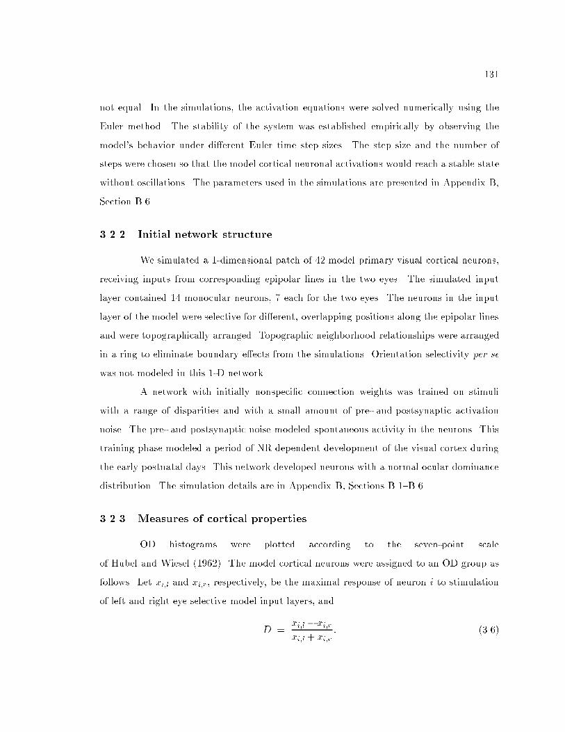
131not equal. In the simulations, the activation equations were solved numerically using theEuler method. The stability of the system was established empirically by observing themodel's behavior under di�erent Euler time step sizes. The step size and the number ofsteps were chosen so that the model cortical neuronal activations would reach a stable statewithout oscillations. The parameters used in the simulations are presented in Appendix B,Section B.6.3.2.2 Initial network structureWe simulated a 1-dimensional patch of 42 model primary visual cortical neurons,receiving inputs from corresponding epipolar lines in the two eyes. The simulated inputlayer contained 14 monocular neurons, 7 each for the two eyes. The neurons in the inputlayer of the model were selective for di�erent, overlapping positions along the epipolar linesand were topographically arranged. Topographic neighborhood relationships were arrangedin a ring to eliminate boundary e�ects from the simulations. Orientation selectivity per sewas not modeled in this 1-D network.A network with initially nonspeci�c connection weights was trained on stimuliwith a range of disparities and with a small amount of pre- and postsynaptic activationnoise. The pre- and postsynaptic noise modeled spontaneous activity in the neurons. Thistraining phase modeled a period of NR dependent development of the visual cortex duringthe early postnatal days. This network developed neurons with a normal ocular dominancedistribution. The simulation details are in Appendix B, Sections B.1{B.6.3.2.3 Measures of cortical propertiesOD histograms were plotted according to the seven-point scaleof Hubel and Wiesel (1962). The model cortical neurons were assigned to an OD group asfollows. Let xi;l and xi;r, respectively, be the maximal response of neuron i to stimulationof left and right eye selective model input layers, andD = xi;l � xi;rxi;l + xi;r : (3.6)

132Then the neuron is assigned to group 1 if 1 � D > 0:80, group 2 if 0:80 � D > 0:45,group 3 if 0:45 � D > 0:10, group 4 if 0:10 � D > �0:10, group 5 if �0:10 � D > �0:45,group 6 if �0:45 � D > �0:80, and group 7 if �0:80 � D � �1. Non-uniform bin sizeswith smaller bins for groups 1, 4, and 7 than for groups 2, 3, 5, and 6 were chosen ratherthan uniform bin sizes, because the former provides a stricter condition to be a member ofgroup 1 (neurons respond to only to the left eye), group 4 (neurons respond equally to botheyes), and group 7 (neurons respond to only to the right eye).Changes in OD were expressed by a contralateral bias index (CBI)CBI = 100� (N1 � N7) + (2=3) (N2 � N6) + (1=3) (N3 � N5) + N2N ; (3.7)where Ni represents the number of neurons in OD group i, and N is the total number ofvisually responsive neurons (Reiter & Stryker, 1988). The fraction of binocular neurons wasmeasured by the binocularity index (BI)BI = N3 +N4 + N5N (3.8)(Bear et al., 1990).The receptive �eld width of left- and right-eye RFs of model cortical neurons weremeasured by width at half-height. Positional selectivity is the reciprocal of RF width.3.3 ResultsThe EXIN rules modeled the e�ects of classical rearing paradigms. An explanationbased on synaptic modi�cations governed by the EXIN rules is provided for normalbinocular vision, monocular deprivation, binocular deprivation, reverse suture, strabimus,and restoration of normal binocular vision after various kinds of deprivation.3.3.1 Normal rearingFigure 3.1 shows the OD distribution of model cortical neurons after normalrearing. The �gure also shows the average maximal responsiveness to monocular stimulationover all the neurons and the average left- and right eye RF width over all the neurons. The

1331.17

L

1.21

R

Avg

. RF

wid

th

0

1

2

3

1 2

1

3

38

4

3

5 6 7 UR0

5

10

15

20

25

30

35

40

45

50N

umbe

r of

neu

rons

Ocular dominanceCBI = 49.21, BI = 1.00

1.89

B

0.66

L

0.66

R

Avg

. res

pons

e X

10

0.00

0.50

1.00

1.50

2.00

Figure 3.1: Normal rearing.B represents binocular inputs, and L and R represent left and right eye monocular inputs.Average responsiveness is the average maximal responses over all the model cortical neuronsneurons. UR represents the unresponsive neurons. The vertical lines on the bars representthe standard deviation, and the numbers above the bars represent the mean values. Thesimulation parameters are described in Section 3.2.4.RF of model cortical neurons and the network pathway weights were stable after 1,500,000presentations of binocular inputs during NR (see Appendix B, Section B.4). Figure 3.2shows the development of left- and right eye RFs of two di�erent model cortical neuronsduring NR. In the model, cortical neurons may become selective for non-correspondingleft- and right eye positions (Figure 3.2a), and therefore, to a particular disparity, becauseof disparity in the training inputs.Factors a�ecting binocularity, responsiveness, and RF width during NRThe binocularity of model cortical neurons decreased as the range of disparity inthe binocular inputs for NR was increased (Figure 3.3). As the range of disparity in theNR inputs is increased, the maximal correlation in the activation of model left and right

134Num

ber o

f iter

ation

s (x 5

000)

0

0

100

200

-1

0

1

2

3

4

5

6

7

Neu

rona

l res

pons

e

Right eye X position

Numbe

r of it

erat

ions (

x 500

0)

0

0

100

200

-1

0

1

2

3

4

5

6

7

Neu

rona

l res

pons

e

Left eye X position

(a)

Numbe

r of it

erat

ions (

x 500

0)

0

0

100

200

-1

0

1

2

3

4

5

6

7

Neu

rona

l res

pons

e

Right eye X position

Numbe

r of it

erat

ions (

x 500

0)

0

0

100

200

-1

0

1

2

3

4

5

6

7

Neu

rona

l res

pons

e

Left eye X position

(b)Figure 3.2: Development of monocular RFs during NR.The �gure shows the development of the left and right RFs of two model cortical neurons.The network was trained with 1,500,000 binocular inputs. The simulation parameters usedare given in Section 3.2.4.

1350.96

L

1.08

R

Avg

. RF

wid

th

0

1

2

3

1

2

2

10

3

16

4

14

5 6 7 UR0

5

10

15

20

25

30

35

40

45

50N

umbe

r of

neu

rons

Ocular dominanceCBI = 50.00, BI = 0.95

0.70

L

0.65

R

Avg

. res

pons

e X

10

0.00

0.50

1.00

1.50

2.00

Figure 3.3: NR with binocular inputs over a larger disparity range.Binocular inputs with disparity in f�4;�10=3;�8=3;�2;�4=3;�2=3; 0; 2=3; 4=3; 2; 8=3; 10=3;4g were used in this simulation. Other simulation parameters were the same as those usedfor the simulation in Figure 3.1. The conventions are the same as in Figure 3.1.eye selective input neurons decreases. If only zero disparity were allowed, the activation ofcorresponding positions in the left and right eye would be fully correlated. For non-zerodisparity ranges, a position in one eye can be coactivated with any position in the othereye allowed by the disparity range. Assuming that all the disparities within the rangeare equally probable, as the disparity range increases the maximal correlation between theactivation of input positions in the two eyes decreases. Furthermore, the correlation in theactivation of model cortical neurons and monocular input neurons decreases.When the correlation between the activation of a model cortical neuron and abinocular pattern of activation of input neurons is high, the model cortical neuron becomesbinocular; the model cortical neuron is activated by a small range of binocular inputsclose to its preferred stimuli and is unresponsive to other inputs. Thus, when a modelcortical neuron is active, the correlation in the activation of left and right eye selectiveinput neurons is high. According to the EXIN a�erent excitatory synaptic plasticity rule,

136plasticity occurs only when model cortical neurons are active. Thus, the model corticalneuron remains binocular.As the number of binocular input patterns activating the neuron increases, themodel cortical neuron can be activated by input stimulation in one RF (e.g., left eye RF)and input stimulation over a range of positions in the other eye. In this case, when a modelcortical neuron is active, the correlation in the activation of monocular input neurons is low.According to the EXIN a�erent excitatory synaptic plasticity rule, unstimulated a�erentexcitatory pathways to active model cortical neurons weaken, and strongly stimulateda�erent excitatory pathways to active model cortical neurons strengthen. Thus, a�erentexcitatory pathways from one eye may weaken in competition with a�erent pathwaysfrom the other eye, and model cortical neurons become less binocular. Because modelcortical neurons became biased toward one of the eyes, the variance in the average maximalresponsiveness to monocular inputs and in the average left and right eye RFs increased(Figure 3.3).The binocularity, responsiveness, and RF width are also dependent on the strengthof lateral inhibitory weights. In the simulations, the function Q(x) = min(0:2; V [x]) inEquation 3.1 was manipulated by varying V . As V was decreased, the maximal inhibitoryweight in the network decreased. Parameter V was set to 3 in Figure 3.1, 0.3 in Figure 3.4a,and 0.03 in Figure 3.4b. As V was decreased, maximal responsiveness to monocular inputsand monocular RF width of the model cortical neuron increased (Figure 3.4). At very lowvalues of V the model cortical neurons were less likely to be strongly monocular (compareFigures 3.4a and 3.4b) because the lateral inhibitory pathways were very weak. Thisphenomenon is analogous to the decrease in the number of neurons responsive exclusivelyto the eye that was open during MD, after a reduction in intracortical inhibition inducedby cortical infusion of a GABA antagonist in kittens that were previously deprived of visionin one eye (Sillito et al., 1981).As V was decreased, lateral inhibitory pathways weakened, thereby decreasingpositional selectivity of model cortical neurons, i.e., their RF width increased. Because oflow selectivity, model cortical neurons were actived by a larger number of binocular inputs,and as in the case of increasing disparity range in the training inputs, the model cortical

1371.54

L

1.64

R

Avg

. RF

wid

th

0

1

2

3

(a)

10

1

10

2

1

3 4

1

5

11

6

9

7 UR0

5

10

15

20

25

30

35

40

45

50N

umbe

r of

neu

rons

Ocular dominanceCBI = 50.40, BI = 0.05

0.68

L

0.67

R

Avg

. res

pons

e X

10

0.00

0.50

1.00

1.50

2.00

2.14

L

2.23

R

Avg

. RF

wid

th

0

1

2

3

(b)

1

21

2 3 4

4

5

17

6 7 UR0

5

10

15

20

25

30

35

40

45

50

Num

ber

of n

euro

ns

Ocular dominanceCBI = 51.59, BI = 0.10

1.22

L

1.21

R

Avg

. res

pons

e X

10

0.00

0.50

1.00

1.50

2.00

Figure 3.4: The e�ects of varying the inhibitory weights during NR.The simulation parameters are the same as for the simulation in Figure 3.1, except thatQ(x) = min(0:2; 0:3[x]) in (a), and Q(x) = min(0:2; 0:03[x]) in (b). The conventions aregiven in Figure 3.1.

138neurons became less binocular. Because model cortical neurons became biased toward oneof the eyes, the variance in the average maximal responsiveness to monocular inputs and inthe average left and right eye RFs increased (Figure 3.4).In the simulations, model cortical neurons were biased to become tunedto binocular inputs because of the square non-linearity in the excitation equation(Equation 3.4), and in the EXIN a�erent excitatory plasticity rule (Equation 3.2). Thesquaring in Equation 3.4 caused model cortical neurons to be more responsive when theyreceived preferred binocular inputs, and the squaring in Equation 3.2 caused the more activeneurons to learn faster. Since preferred binocular inputs activate model cortical neuronsmore strongly than other inputs, the excitatory plasticity rule caused the active neuronsto learn the preferred stimuli faster than the less preferred inputs. Thus, the unlearningthat occurs when less preferred stimuli active model cortical neurons is o�set by the fasterlearning that occurs when the preferred stimuli is presented.3.3.2 Monocular deprivationIn the model, MD resulted in OD shift toward the open eye (the left eye inFigure 3.5). Figure 3.6 shows the changes in the left and right RFs of two model corticalneurons during MD.Stimulation of the open eye activates model cortical neurons. According to theexcitatory synaptic plasticity rule, the synaptic weights of a�erent excitatory pathwaysfrom the open eye selective active monocular input neurons increase, and the synapticweights of a�erent excitatory pathways from the inactive closed eye selective monocularinput neurons decrease. Thus, the a�erent excitatory pathway weights from the closedeye selective monocular input neurons to model cortical neurons eventually decay to lowrandom values.In the simulations, the average maximal responsiveness of model cortical neuronsto the open eye stimulation increased, and the average maximal responsiveness ofmodel cortical neurons to the closed eye stimulation decreased (Figures 3.5 and 3.6).Increase in responsiveness to the open eye has been observed in MD experiments(Mioche & Singer, 1989). The average width of the closed eye RFs of model cortical neurons

1391.13

L

1.22

R

Avg

. RF

wid

th

0

1

2

3

1 2

18

3

23

4

1

5 6 7 UR0

5

10

15

20

25

30

35

40

45

50

Num

ber

of n

euro

ns

Ocular dominance

18,750 iterations

CBI = 56.75, BI = 1.00

0.66

L

0.56

R

Avg

. res

pons

e X

10

0.00

0.50

1.00

1.50

2.00

1.10

L

1.11

R

Avg

. RF

wid

th

0

1

2

3

1 2

41

3 4

1

5 6 7 UR0

5

10

15

20

25

30

35

40

45

50

Num

ber

of n

euro

ns

Ocular dominance

37,500 iterations

CBI = 65.87, BI = 1.00

0.67

L

0.44

R

Avg

. res

pons

e X

10

0.00

0.50

1.00

1.50

2.00

1.13

L

1.06

R

Avg

. RF

wid

th

0

1

2

3

1

14

2

27

3

1

4 5 6 7 UR0

5

10

15

20

25

30

35

40

45

50

Num

ber

of n

euro

ns

Ocular dominance

56,250 iterations

CBI = 71.83, BI = 0.67

0.69

L

0.31

R

Avg

. res

pons

e X

10

0.00

0.50

1.00

1.50

2.00

1.13

L

1.05

RA

vg. R

F w

idth

0

1

2

3

1

41

2

1

3 4 5 6 7 UR0

5

10

15

20

25

30

35

40

45

50

Num

ber

of n

euro

ns

Ocular dominance

75,000 iterations

CBI = 82.94, BI = 0.02

0.70

L

0.19

R

Avg

. res

pons

e X

10

0.00

0.50

1.00

1.50

2.00

Figure 3.5: OD changes during MD.The parameters are given in Section 3.2.4, and the conventions are in Figure 3.1. The lefteye was the open eye and the right eye was closed.

140Num

ber o

f iter

ation

s (x 5

000)

0

010

-1

0

1

2

3

4

5

6

7

Neu

rona

l res

pons

eRight eye X position

Numbe

r of it

erat

ions (

x 500

0)

0

010

-1

0

1

2

3

4

5

6

7

Neu

rona

l res

pons

e

Left eye X position

(a)Num

ber o

f iter

ation

s (x 5

000)

0

010

-1

0

1

2

3

4

5

6

7

Neu

rona

l res

pons

e

Right eye X position

Numbe

r of it

erat

ions (

x 500

0)

0

010

-1

0

1

2

3

4

5

6

7

Neu

rona

l res

pons

e

Left eye X position

(b)Figure 3.6: Monocular RF changes during MD.The parameters are given in Section 3.2.4. The left eye was the open eye and the right eyewas closed.

1411.00

L

0.82

R

Avg

. RF

wid

th

0

1

2

3

12

1

16

2

2

3

5

4

1

5 6

6

7 UR0

5

10

15

20

25

30

35

40

45

50

Num

ber

of n

euro

ns

Ocular dominance

125,000 iterations

CBI = 70.24, BI = 0.19

0.60

L

0.69

RA

vg. r

espo

nse

X 1

00.00

0.50

1.00

1.50

2.00

0.79

L

0.78

R

Avg

. RF

wid

th

0

1

2

3

13

1

8

2

6

3 4

2

5 6

13

7 UR0

5

10

15

20

25

30

35

40

45

50

Num

ber

of n

euro

ns

Ocular dominance

250,000 iterations

CBI = 57.94, BI = 0.19

0.52

L

0.99

R

Avg

. res

pons

e X

10

0.00

0.50

1.00

1.50

2.00

0.75

L

0.75

R

Avg

. RF

wid

th

0

1

2

3

14

1

5

2

2

3

1

4

3

5

1

6

16

7 UR0

5

10

15

20

25

30

35

40

45

50

Num

ber

of n

euro

ns

Ocular dominance

375,000 iterations

CBI = 50.40, BI = 0.14

0.45

L

0.86

R

Avg

. res

pons

e X

10

0.00

0.50

1.00

1.50

2.00

0.69

L

0.79

R

Avg

. RF

wid

th

0

1

2

3

16

1 2

4

3 4

1

5

2

6

19

7 UR0

5

10

15

20

25

30

35

40

45

50

Num

ber

of n

euro

ns

Ocular dominance

500,000 iterations

CBI = 46.03, BI = 0.12

0.40

L

0.77

R

Avg

. res

pons

e X

10

0.00

0.50

1.00

1.50

2.00

Figure 3.7: OD changes during RS.The parameters are given in Section 3.2.4, and the conventions are in Figure 3.1. The righteye was the open eye and the left eye was closed.decreased, and the variance in the average width increased (Figure 3.5).3.3.3 Reverse sutureIn RS, the stimulation of the eyes was reversed following MD in Section 3.3.2;i.e., the left eye received low, random inputs, and the right eye received monocularstimulation. During RS, OD of model cortical neurons shifted toward the newly opened eye(Figures 3.7 and 3.8).Immediately after the reversal of the input presentation to the two eyes, modelcortical neurons are weakly activated because the a�erent excitatory pathways with strongweights receive low, random inputs, and the input patterns are presented to the monocular

142Num

ber o

f iter

ation

s (x 5

000)

0

0

50

-1

0

1

2

3

4

5

6

7

Neu

rona

l res

pons

eRight eye X position

Numbe

r of it

erat

ions (

x 500

0)

0

0

50

-1

0

1

2

3

4

5

6

7

Neu

rona

l res

pons

e

Left eye X position

(a)Num

ber o

f iter

ation

s (x 5

000)

0

0

50

-1

0

1

2

3

4

5

6

7

Neu

rona

l res

pons

e

Right eye X position

Numbe

r of it

erat

ions (

x 500

0)

0

0

50

-1

0

1

2

3

4

5

6

7

Neu

rona

l res

pons

e

Left eye X position

(b)Figure 3.8: Monocular RF changes during RS.The parameters are given in Section 3.2.4. The right eye was the open eye and the left eyewas closed.

143Num

ber o

f iter

ation

s (x 5

000)

0

0

100

200

-1

0

1

2

3

4

5

6

7

Neu

rona

l res

pons

e

Right eye X position

Numbe

r of it

erat

ions (

x 500

0)

0

0

100

200

-1

0

1

2

3

4

5

6

7

Neu

rona

l res

pons

e

Left eye X position

(a)

Numbe

r of it

erat

ions (

x 500

0)

0

0

100

200

-1

0

1

2

3

4

5

6

7

Neu

rona

l res

pons

e

Right eye X position

Numbe

r of it

erat

ions (

x 500

0)

0

0

100

200

-1

0

1

2

3

4

5

6

7

Neu

rona

l res

pons

e

Left eye X position

(b)Figure 3.9: Monocular RF changes during NR for the neurons in Figure 3.8.Figures (a) and (b) show the monocular RFs of the neurons whose monocular RFs are shownin Figures 3.8a and 3.8b, respectively, during NR. The parameters are given in Section 3.2.4.

144input layer with weak a�erent pathways to model cortical neurons. Low activation ofmodel cortical neurons causes slow changes in the a�erent excitatory pathways. The initiallarge a�erent pathway weights from the left eye selective input layer to the model corticalneurons are decreased every time model cortical neurons are actived. Simultaneously, modelcortical neurons strengthen a�erent excitatory pathways from the right eye selective inputlayer. The temporal competition among the various input patterns slows the developmentof strong a�erent excitatory pathways from the right eye selective input neurons comparedto the decay of a�erent excitatory pathway weights between the left eye selective inputneurons and model cortical neurons. Thus, in the simulations, model cortical neurons lostresponsiveness to the newly closed eye before becoming responsive to the newly opened eye(Figure 3.8).During RS, some neurons became highly responsive to the newly opened eye(Figure 3.8b). Because of the lateral inhibitory interactions, high responsiveness of someneurons to the newly opened eye caused complete suppression of responsiveness of othermodel cortical neurons to the newly opened eye, thereby increasing the number of neuronsresponsive only to the previously closed eye (Figure 3.7). A low activation level of modelcortical neurons weakens the lateral inhibitory weights to the neurons according to the EXINlateral inhibitory synaptic plasticity rule. In the simulation, the decrease in inhibitoryweights increased the responsiveness of inactive neurons to the newly opened eye andeventually caused the neurons to become responsive exclusively to the newly opened eye(Figure 3.8a).During RS, the average maximal responsiveness of model cortical neurons to thenewly opened eye increased (Figure 3.7), and the average maximal responsiveness of modelcortical neurons to the newly closed eye decreased (Figure 3.7). The variance in the maximalresponsiveness of model cortical neurons to the newly opened eye was large; some neuronsbecame highly responsive to the newly opened eye (Figure 3.8b) because of weakening ofthe lateral inhibitory pathways. In addition, most neurons responded to the left or theright eye; therefore, the maximal responsiveness of model cortical neurons to monocularstimulation varied widely.In the MD simulation described in Section 3.3.2, model cortical neurons did not

145completely lose their responsiveness to the closed eye (Figures 3.5 and 3.6). Therefore,during the subsequent RS conditioning, the RF tuning of the model cortical neurons for thenewly opened eye was close to the neurons' original RF tuning in the same eye after NR(compare the right-eye RFs in Figures 3.8 and 3.9).3.3.4 StrabismusDuring ST, the left and right inputs were uncorrelated, and the model corticalneurons became selective for correlated patterns of activation in the monocular input layers.Thus, the model cortical neurons became monocular (Figures 3.10 and 3.11). The modelcortical neurons became selective for positions in the left or right eye (Figure 3.11).After ST, model cortical neurons responded to the left or the right eye. Thus,the monocular RF width and the maximal responsiveness of model cortical neurons tomonocular stimulation varied widely, and the variance in the maximal responsiveness tomonocular inputs, and in the monocular RF widths was high (Figure 3.10). During ST,some neurons became highly responsive (Figure 3.11b).3.3.5 Binocular deprivationAfter prolonged BD, the average maximal responsiveness to monocular inputsdecreased, the average monocular RF width increased, and model cortical neurons remainedbinocular (Figure 3.12). During BD, the input neurons received very weak noisy activation,and according to the excitatory synaptic plasticity rule, unstimulated and weakly stimulateda�erent excitatory pathways to active neurons weaken. The noise in the input activatesmodel cortical neurons very weakly. To speed up the rate of weakening of the a�erentexcitatory pathways, a random-noise term was included in the excitatory synaptic plasticityrule (Appendix B, Section B.6).The EXIN lateral inhibitory synaptic plasticity rule is instrumental in wideningthe monocular RFs. Since model cortical neurons are very weakly activated during BD, thelateral inhibitory pathways are weakened. Weakened lateral inhibitory pathways increasedthe RF width (decreased position selectivity) of model cortical neurons (Figure 3.12).When lateral inhibitory synaptic plasticity was disabled during BD, the average maximal

1460.78

L

0.76

R

Avg

. RF

wid

th

0

1

2

3

17

1

2

2

1

3 4

4

5

1

6

17

7 UR0

5

10

15

20

25

30

35

40

45

50

Num

ber

of n

euro

ns

Ocular dominance

125,000 iterations

CBI = 49.60, BI = 0.12

0.57

L

0.54

RA

vg. r

espo

nse

X 1

00.00

0.50

1.00

1.50

2.00

0.63

L

0.69

R

Avg

. RF

wid

th

0

1

2

3

19

1 2

1

3 4 5 6

22

7 UR0

5

10

15

20

25

30

35

40

45

50

Num

ber

of n

euro

ns

Ocular dominance

250,000 iterations

CBI = 46.83, BI = 0.02

0.65

L

0.63

R

Avg

. res

pons

e X

10

0.00

0.50

1.00

1.50

2.00

0.50

L

0.59

R

Avg

. RF

wid

th

0

1

2

3

19

1 2

1

3 4 5 6

22

7 UR0

5

10

15

20

25

30

35

40

45

50

Num

ber

of n

euro

ns

Ocular dominance

375,000 iterations

CBI = 46.83, BI = 0.02

0.65

L

0.66

R

Avg

. res

pons

e X

10

0.00

0.50

1.00

1.50

2.00

0.50

L

0.58

R

Avg

. RF

wid

th

0

1

2

3

19

1 2

1

3 4 5 6

22

7 UR0

5

10

15

20

25

30

35

40

45

50

Num

ber

of n

euro

ns

Ocular dominance

500,000 iterations

CBI = 46.83, BI = 0.02

0.65

L

0.66

R

Avg

. res

pons

e X

10

0.00

0.50

1.00

1.50

2.00

Figure 3.10: OD changes during ST.The parameters are given in Section 3.2.4, and the conventions are in Figure 3.1.responsiveness of model cortical neurons to monocular stimulation decreased, but themonocular RF widths of model cortical neurons also decreased (Figure 3.14).3.3.6 RecoveryIn the EXIN model, presentation of normal, binocular inputs followingMD (Figures 3.15 and 3.16), ST (Figures 3.17 and 3.18), and BD (Figures 3.20 and 3.21)restored the OD distribution, the average maximal responsiveness of neurons to monocularinputs, and the average monocular RF widths.During the prolonged BD in Section 3.3.5, the model cortical neurons became veryweakly responsive to both eyes and lost their positional selectivity (Figures 3.12 and 3.13).During the subsequent normal training, model cortical neurons became selective for di�erent

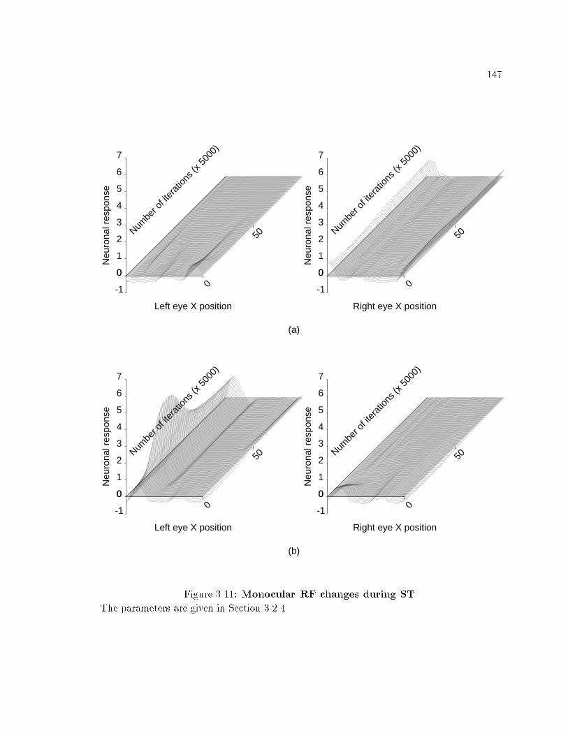
147Num

ber o

f iter

ation

s (x 5

000)

0

0

50

-1

0

1

2

3

4

5

6

7

Neu

rona

l res

pons

eRight eye X position

Numbe

r of it

erat

ions (

x 500

0)

0

0

50

-1

0

1

2

3

4

5

6

7

Neu

rona

l res

pons

e

Left eye X position

(a)Num

ber o

f iter

ation

s (x 5

000)

0

0

50

-1

0

1

2

3

4

5

6

7

Neu

rona

l res

pons

e

Right eye X position

Numbe

r of it

erat

ions (

x 500

0)

0

0

50

-1

0

1

2

3

4

5

6

7

Neu

rona

l res

pons

e

Left eye X position

(b)Figure 3.11: Monocular RF changes during ST.The parameters are given in Section 3.2.4.

1481.28

L

1.26

R

Avg

. RF

wid

th

0

1

2

3

1 2 3

42

4 5 6 7 UR0

5

10

15

20

25

30

35

40

45

50

Num

ber

of n

euro

ns

Ocular dominance

1,250,000 iterations

CBI = 50.00, BI = 1.00

0.50

L

0.51

R

Avg

. res

pons

e X

10

0.00

0.50

1.00

1.50

2.00

1.50

L

1.40

R

Avg

. RF

wid

th

0

1

2

3

1 2 3

42

4 5 6 7 UR0

5

10

15

20

25

30

35

40

45

50

Num

ber

of n

euro

nsOcular dominance

2,500,000 iterations

CBI = 50.00, BI = 1.00

0.21

L

0.21

R

Avg

. res

pons

e X

10

0.00

0.50

1.00

1.50

2.00

1.60

L

1.61

R

Avg

. RF

wid

th

0

1

2

3

1 2 3

42

4 5 6 7 UR0

5

10

15

20

25

30

35

40

45

50

Num

ber

of n

euro

ns

Ocular dominance

3,750,000 iterations

CBI = 50.00, BI = 1.00

0.05

L

0.05

R

Avg

. res

pons

e X

10

0.00

0.50

1.00

1.50

2.00

1.60

L

1.63

RA

vg. R

F w

idth

0

1

2

3

1 2 3

42

4 5 6 7 UR0

5

10

15

20

25

30

35

40

45

50

Num

ber

of n

euro

ns

Ocular dominance

5,000,000 iterations

CBI = 50.00, BI = 1.00

0.01

L

0.01

R

Avg

. res

pons

e X

10

0.00

0.50

1.00

1.50

2.00

Figure 3.12: OD changes during BD.The parameters are given in Section 3.2.4, and the conventions are in Figure 3.1.

149Num

ber o

f iter

ation

s (x 5

000)

0

0

500

-1

0

1

2

3

4

5

6

7

Neu

rona

l res

pons

eRight eye X position

Numbe

r of it

erat

ions (

x 500

0)

0

0

500

-1

0

1

2

3

4

5

6

7

Neu

rona

l res

pons

e

Left eye X position

(a)Num

ber o

f iter

ation

s (x 5

000)

0

0

500

-1

0

1

2

3

4

5

6

7

Neu

rona

l res

pons

e

Right eye X position

Numbe

r of it

erat

ions (

x 500

0)

0

0

500

-1

0

1

2

3

4

5

6

7

Neu

rona

l res

pons

e

Left eye X position

(b)Figure 3.13: Monocular RF changes during BD.The parameters are given in Section 3.2.4.

1500.90

L

0.83

R

Avg

. RF

wid

th

0

1

2

3

1 2

11

3

25

4

6

5 6 7 UR0

5

10

15

20

25

30

35

40

45

50

Num

ber

of n

euro

ns

Ocular dominance

1,250,000 iterations

CBI = 51.98, BI = 1.00

0.25

L

0.24

R

Avg

. res

pons

e X

10

0.00

0.50

1.00

1.50

2.00

0.74

L

0.74

R

Avg

. RF

wid

th

0

1

2

3

1 2

14

3

17

4

11

5 6 7 UR0

5

10

15

20

25

30

35

40

45

50

Num

ber

of n

euro

ns

Ocular dominance

2,500,000 iterations

CBI = 51.19, BI = 1.00

0.07

L

0.07

R

Avg

. res

pons

e X

10

0.00

0.50

1.00

1.50

2.00

0.70

L

0.64

R

Avg

. RF

wid

th

0

1

2

3

1 2

15

3

15

4

12

5 6 7 UR0

5

10

15

20

25

30

35

40

45

50

Num

ber

of n

euro

ns

Ocular dominance

3,750,000 iterations

CBI = 51.19, BI = 1.00

0.01

L

0.01

R

Avg

. res

pons

e X

10

0.00

0.50

1.00

1.50

2.00

0.62

L

0.60

RA

vg. R

F w

idth

0

1

2

3

1 2

14

3

16

4

12

5 6 7 UR0

5

10

15

20

25

30

35

40

45

50

Num

ber

of n

euro

ns

Ocular dominance

5,000,000 iterations

CBI = 50.79, BI = 1.00

0.00

L

0.00

R

Avg

. res

pons

e X

10

0.00

0.50

1.00

1.50

2.00

Figure 3.14: Monocular RF changes during BD without lateral inhibitorysynaptic plasticity.The parameters are the same as those in the simulation in Figure 3.11 except that thelateral inhibitory synaptic plasticity was blocked.

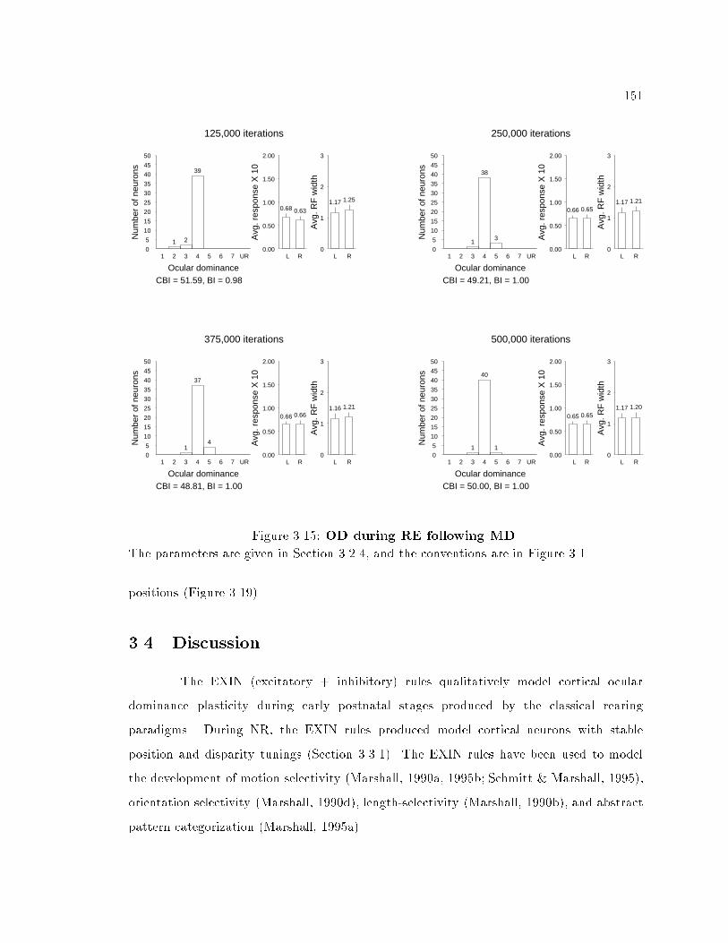
1511.17

L

1.25

R

Avg

. RF

wid

th

0

1

2

3

1

1

2

2

3

39

4 5 6 7 UR0

5

10

15

20

25

30

35

40

45

50

Num

ber

of n

euro

ns

Ocular dominance

125,000 iterations

CBI = 51.59, BI = 0.98

0.68

L

0.63

RA

vg. r

espo

nse

X 1

00.00

0.50

1.00

1.50

2.00

1.17

L

1.21

R

Avg

. RF

wid

th

0

1

2

3

1 2

1

3

38

4

3

5 6 7 UR0

5

10

15

20

25

30

35

40

45

50

Num

ber

of n

euro

ns

Ocular dominance

250,000 iterations

CBI = 49.21, BI = 1.00

0.66

L

0.65

R

Avg

. res

pons

e X

10

0.00

0.50

1.00

1.50

2.00

1.16

L

1.21

R

Avg

. RF

wid

th

0

1

2

3

1 2

1

3

37

4

4

5 6 7 UR0

5

10

15

20

25

30

35

40

45

50

Num

ber

of n

euro

ns

Ocular dominance

375,000 iterations

CBI = 48.81, BI = 1.00

0.66

L

0.66

R

Avg

. res

pons

e X

10

0.00

0.50

1.00

1.50

2.00

1.17

L

1.20

R

Avg

. RF

wid

th

0

1

2

3

1 2

1

3

40

4

1

5 6 7 UR0

5

10

15

20

25

30

35

40

45

50

Num

ber

of n

euro

ns

Ocular dominance

500,000 iterations

CBI = 50.00, BI = 1.00

0.65

L

0.65

R

Avg

. res

pons

e X

10

0.00

0.50

1.00

1.50

2.00

Figure 3.15: OD during RE following MD.The parameters are given in Section 3.2.4, and the conventions are in Figure 3.1.positions (Figure 3.19).3.4 DiscussionThe EXIN (excitatory + inhibitory) rules qualitatively model cortical oculardominance plasticity during early postnatal stages produced by the classical rearingparadigms. During NR, the EXIN rules produced model cortical neurons with stableposition and disparity tunings (Section 3.3.1). The EXIN rules have been used to modelthe development of motion selectivity (Marshall, 1990a, 1995b; Schmitt & Marshall, 1995),orientation selectivity (Marshall, 1990d), length-selectivity (Marshall, 1990b), and abstractpattern categorization (Marshall, 1995a).

152Num

ber o

f iter

ation

s (x 5

000)

0

0

50

-1

0

1

2

3

4

5

6

7

Neu

rona

l res

pons

eRight eye X position

Numbe

r of it

erat

ions (

x 500

0)

0

0

50

-1

0

1

2

3

4

5

6

7

Neu

rona

l res

pons

e

Left eye X position

(a)Num

ber o

f iter

ation

s (x 5

000)

0

0

50

-1

0

1

2

3

4

5

6

7

Neu

rona

l res

pons

e

Right eye X position

Numbe

r of it

erat

ions (

x 500

0)

0

0

50

-1

0

1

2

3

4

5

6

7

Neu

rona

l res

pons

e

Left eye X position

(b)Figure 3.16: Monocular RF changes during RE following MD.The parameters are given in Section 3.2.4.

1530.90

L

0.87

R

Avg

. RF

wid

th

0

1

2

3

1 2

2

3

30

4

1

5 6 7

9

UR0

5

10

15

20

25

30

35

40

45

50

Num

ber

of n

euro

ns

Ocular dominance

1,250,000 iterations

CBI = 50.51, BI = 1.00

0.61

L

0.61

RA

vg. r

espo

nse

X 1

00.00

0.50

1.00

1.50

2.00

1.10

L

1.14

R

Avg

. RF

wid

th

0

1

2

3

1 2

9

3

24

4

9

5 6 7 UR0

5

10

15

20

25

30

35

40

45

50

Num

ber

of n

euro

ns

Ocular dominance

2,500,000 iterations

CBI = 50.00, BI = 1.00

0.68

L

0.65

R

Avg

. res

pons

e X

10

0.00

0.50

1.00

1.50

2.00

1.06

L

1.14

R

Avg

. RF

wid

th

0

1

2

3

1 2

6

3

29

4

7

5 6 7 UR0

5

10

15

20

25

30

35

40

45

50

Num

ber

of n

euro

ns

Ocular dominance

3,750,000 iterations

CBI = 49.60, BI = 1.00

0.67

L

0.66

R

Avg

. res

pons

e X

10

0.00

0.50

1.00

1.50

2.00

1.09

L

1.16

R

Avg

. RF

wid

th

0

1

2

3

1 2

9

3

27

4

6

5 6 7 UR0

5

10

15

20

25

30

35

40

45

50

Num

ber

of n

euro

ns

Ocular dominance

5,000,000 iterations

CBI = 51.19, BI = 1.00

0.67

L

0.66

R

Avg

. res

pons

e X

10

0.00

0.50

1.00

1.50

2.00

Figure 3.17: OD during RE following BD.The parameters are given in Section 3.2.4, and the conventions are in Figure 3.1.The EXIN rules also produced the following salient features of OD plasticity afterMD, RS, ST, BD, and RE consistent with the experimental results reviewed in Section 3.1.� OD shift toward the open eye after MD; model cortical neurons lost responsivenessto the closed eye and gained responsiveness to the open eye.� OD shift toward the newly opened eye after RS; model cortical neurons lostresponsiveness to the newly closed eye before gaining responsiveness to the newlyopened eye.� Loss of binocularity after ST; model cortical neurons became responsive exclusivelyto one of the eyes.� Loss of responsiveness to both eyes without loss of binocularity, and loss of position

154Num

ber o

f iter

ation

s (x 5

000)

0

0

500

-1

0

1

2

3

4

5

6

7

Neu

rona

l res

pons

eRight eye X position

Numbe

r of it

erat

ions (

x 500

0)

0

0

500

-1

0

1

2

3

4

5

6

7

Neu

rona

l res

pons

e

Left eye X position

(a)Num

ber o

f iter

ation

s (x 5

000)

0

0

500

-1

0

1

2

3

4

5

6

7

Neu

rona

l res

pons

e

Right eye X position

Numbe

r of it

erat

ions (

x 500

0)

0

0

500

-1

0

1

2

3

4

5

6

7

Neu

rona

l res

pons

e

Left eye X position

(b)Figure 3.18: Monocular RF changes during RE following BD.The parameters are given in Section 3.2.4.

155Num

ber o

f iter

ation

s (x 5

000)

0

0

500

-1

0

1

2

3

4

5

6

7

Neu

rona

l res

pons

e

Right eye X position

Numbe

r of it

erat

ions (

x 500

0)

0

0

500

-1

0

1

2

3

4

5

6

7

Neu

rona

l res

pons

e

Left eye X position

(a)

Numbe

r of it

erat

ions (

x 500

0)

0

0

100

200

-1

0

1

2

3

4

5

6

7

Neu

rona

l res

pons

e

Right eye X position

Numbe

r of it

erat

ions (

x 500

0)

0

0

100

200

-1

0

1

2

3

4

5

6

7

Neu

rona

l res

pons

e

Left eye X position

(b)Figure 3.19: Monocular RF changes during RE following prolonged BD andduring NR.The �gure shows the RF tuning of a model cortical neuron during RE following prolongedBD (a) and during NR (b). The neuron did not recover its original position selectivity afternormal training following prolonged BD. The parameters are given in Section 3.2.4.

1560.61

L

0.68

R

Avg

. RF

wid

th

0

1

2

3

19

1

1

2 3 4 5 6

22

7 UR0

5

10

15

20

25

30

35

40

45

50

Num

ber

of n

euro

ns

Ocular dominance

125,000 iterations

CBI = 47.22, BI = 0.00

0.60

L

0.66

RA

vg. r

espo

nse

X 1

00.00

0.50

1.00

1.50

2.00

0.87

L

1.02

R

Avg

. RF

wid

th

0

1

2

3

3

1

3

2

10

3

8

4

15

5

3

6 7 UR0

5

10

15

20

25

30

35

40

45

50

Num

ber

of n

euro

ns

Ocular dominance

250,000 iterations

CBI = 51.59, BI = 0.79

0.70

L

0.66

R

Avg

. res

pons

e X

10

0.00

0.50

1.00

1.50

2.00

1.02

L

1.04

R

Avg

. RF

wid

th

0

1

2

3

1

3

2

6

3

25

4

8

5 6 7 UR0

5

10

15

20

25

30

35

40

45

50

Num

ber

of n

euro

ns

Ocular dominance

375,000 iterations

CBI = 51.59, BI = 0.93

0.70

L

0.67

R

Avg

. res

pons

e X

10

0.00

0.50

1.00

1.50

2.00

1.10

L

1.08

R

Avg

. RF

wid

th

0

1

2

3

1 2

3

3

33

4

6

5 6 7 UR0

5

10

15

20

25

30

35

40

45

50

Num

ber

of n

euro

ns

Ocular dominance

500,000 iterations

CBI = 48.81, BI = 1.00

0.69

L

0.68

R

Avg

. res

pons

e X

10

0.00

0.50

1.00

1.50

2.00

Figure 3.20: OD during RE following ST.The parameters are given in Section 3.2.4, and the conventions are in Figure 3.1.selectivity (i.e., increase in RF width) after prolonged BD.� Restoration of OD distribution, responsiveness, and RF width after normal binocularstimulation following MD and BD. Model cortical neurons became selective to di�erentpositions after RE following prolonged BD.In the EXIN model, OD changes during the classical rearing paradigms dependmainly on the a�erent excitatory synaptic plasticity; the lateral inhibitory synapticplasticity, however, is critical for the development of high input feature selectivity. As shownin Section 3.3.1, weak lateral inhibition produces model cortical neurons with low inputfeature selectivity, which in turn makes the model cortical neurons monocular. Furthermore,lateral inhibitory interactions produce secondary OD changes; when some model cortical

157Num

ber o

f iter

ation

s (x 5

000)

0

0

50

-1

0

1

2

3

4

5

6

7

Neu

rona

l res

pons

eRight eye X position

Numbe

r of it

erat

ions (

x 500

0)

0

0

50

-1

0

1

2

3

4

5

6

7

Neu

rona

l res

pons

e

Left eye X position

(a)Num

ber o

f iter

ation

s (x 5

000)

0

0

50

-1

0

1

2

3

4

5

6

7

Neu

rona

l res

pons

e

Right eye X position

Numbe

r of it

erat

ions (

x 500

0)

0

0

50

-1

0

1

2

3

4

5

6

7

Neu

rona

l res

pons

e

Left eye X position

(b)Figure 3.21: Monocular RF changes during RE following ST.The parameters are given in Section 3.2.4.

158neurons become more responsive to one eye, the inhibitory interaction causes other neuronsto become less responsive to that eye.During NR, the correlation in the stimulation of corresponding locations in thetwo eyes a�ects the OD distribution. In the simulation, as the range of disparity in theleft and right eye stimulation during binocular stimulation was increased, the correlation inthe corresponding locations in the two eyes decreased, and model cortical neurons becameless binocular. During MD, the OD shifted toward the open eye because of weakeningof the a�erent excitatory pathways from the closed eye to the model cortical neurons.In RS, OD shifted toward the newly opened eye because of weakening of a�erent excitatorypathways from the newly closed eye to model cortical neurons and because of strengtheningof a�erent excitatory pathways from the newly opened eye to model cortical neurons. Lateralinhibitory interactions caused the OD of some model cortical neurons to shift toward thenewly closed eye during RS, when some model cortical neurons became highly responsiveto the newly opened eye. In ST, the stimulation patterns of corresponding positions inthe two eyes were uncorrelated, and model cortical neurons became monocular becauseof the competitive a�erent excitatory synaptic plasticity rule. During BD, the a�erentexcitatory synaptic plasticity rule was responsible for a reduction of responsiveness of modelcortical neurons to both eyes, but the lateral inhibitory synaptic rule was responsible forweakening of position selectivity of the model cortical neurons. The a�erent excitatorysynaptic plasticity rule alone during BD reduced responsiveness and increased the positionselectivity of model cortical neurons. Binocular stimulation following MD, BD, and STrestored the OD distribution, responsiveness, and receptive �eld width of model corticalneurons. The a�erent excitatory synaptic plasticity rule restored the a�erent excitatorypathway weights, and lateral inhibitory synaptic plasticity rule ensured high selectivity ofthe model cortical neurons.3.4.1 Role of lateral inhibitory synaptic plasticity on neuronal featureselectivityIt has been proposed that several input feature selectivities depend on intracorticalinhibition (Bonds & DeBruyn, 1985; Sillito, 1975, 1997, 1979; Somers et al., 1995;

159Somogyi & Martin, 1985). The EXIN rules produce neurons with high selectivity andsparse distributed coding (Marshall, 1995a; Marshall & Gupta, 1998). In the EXIN model,strong lateral inhibitory pathways develop between neurons with overlapping receptive �elds(Marshall, 1995a), consistent with experimental results suggesting that a neuron receives thestrongest inhibition when the orientation of the input stimulus is the same as the neuron'spreferred orientation (Blakemore & Tobin, 1972; Ferster, 1989), or when the position of theinput stimulus is in the neuron's receptive �eld (DeAngelis et al., 1992).In the EXIN model, position tuning and orientation tuning can change because ofchanges in either a�erent excitatory pathway or lateral inhibitory pathway weight values.Weakening lateral inhibitory pathways in the model makes neurons more responsive to weakexcitation; neurons can become more responsive to some of the less-preferred orientationsor positions, leading to reduced orientation selectivity and position selectivity.Hendry et al. (1990) reported a decrease in the density of GABAA receptorsin ocular dominance columns corresponding to the closed eye in layer 4C� of adultmonkey primary visual cortex after �ve or ten days of monocular deprivation. Aftermonocular deprivation of adult cats, visual stimulation revealed a lack of lateral inhibitoryinteractions, which are seen in normal cortex, in the monocularly deprived cortex(Kasamatsu et al., 1998b). In neocortical cultures, blockade of spontaneous activityreversibly decreased the number of GABA-positive neurons, decreased GABA-mediatedinhibition onto pyramidal neurons, and raised the �ring rates of pyramidal neurons(Rutherford et al., 1997). The EXIN lateral inhibitory synaptic plasticity rule proposesweakening of inhibition to the inactive neurons, and it is therefore consistent with theabove experimental results.If prolonged BD also causes a decrease in GABA receptors and GABA-positiveneurons during prolonged BD, the EXIN model provides an alternate explanation of thelack of recovery of binocularity of cortical neurons during normal binocular vision followingprolonged BD (Cynader, 1983). Previously, it has been thought that long periods of BDproduces eye misalignment and subsequent loss of correlated inputs to the two eyes whennormal binocular vision is restored, leading to loss of binocularity (Cynader, 19983). Iflateral inhibitory pathways remain weak during binocular vision after prolonged BD, cortical

160neurons can become responsive to one of the eyes, as in the EXIN model with low inhibitorypathway weights (Figure 3.4).3.4.2 Site of cortical OD plasticityIn this paper, cortical OD plasticity is modeled by plasticity in a�erent excitatoryand lateral inhibitory synapses. Changes in cortical OD can be induced by anatomicalchanges in the geniculocortical pathways (LeVay et al., 1980). However, there isalso evidence that OD changes can be induced without a corresponding anatomicalchange in the geniculocortical projections, if MD is initiated late in the critical period(Wiesel, 1982). Furthermore, cortical OD plasticity can occur within four to eight hours(Freeman et al., 1981); the rapid OD plasticity suggests that OD plasticity may involvechanges in the e�cacy of individual cortical synapses. Responsiveness of cortical neuronsto the deprived eye during MD can be restored by abolishing intracortical inhibition,thereby suggesting the involvement of lateral inhibitory interactions in OD plasticity(Sillito et al., 1981).3.4.3 Comparison with other models of cortical OD plasticityPrevious models of OD plasticity (Clothiaux et al., 1991; Miller et al., 1989) arebased on excitatory synaptic plasticity in geniculocortical pathways. Shouval et al. (1996)used the BCM a�erent synaptic plasticity rule to show that misalignment of the two eyescauses model cortical neurons to become monocular. Sirosh and Miikkulainen (1997) useda self-organizing model with a�erent excitatory, lateral excitatory, and lateral inhibitorysynaptic plasticity rules, to model the development of ocular dominance columns and tostudy the relationship between the distribution of lateral excitatory and lateral inhibitorypathways and the ocular dominance and orientation selectivity of model cortical neurons.Sirosh and Miikkulainen (1997) showed that in their model, lateral pathways developbetween cortical neurons with similar properties (e.g., orientation selectivity and oculardominance).The EXIN a�erent excitatory synaptic plasticity rule di�ers from the rules usedby Clothiaux et al. (1991) and Miller et al. (1989).

161Clothiaux et al. (1991) used the BCM (Bienenstock et al., 1982) rule. Accordingto the BCM rule, the synaptic weight of a�erent pathways to cortical neurons variesas a product of input activity and a function (�) of the postsynaptic response. Forall postsynaptic responses greater than the spontaneous activation level but less than amodi�cation threshold (�), � is negative; � is positive when the postsynaptic activationexceeds �. According to the BCM rule, an excitatory pathway synaptic weight is weakenedonly when the pathway receives input stimulation and the postsynaptic activation isless than � and is strengthened only when the pathway receives input stimulation andthe postsynaptic activation is greater than �. The modi�cation threshold � varies asa non-linear function of the average postsynaptic activation (Bienenstock et al., 1982;Clothiaux et al., 1991).An interesting feature of the BCM rule is that weakening of a�erent excitatorypathways from the closed eye to a model cortical neuron during MD depends on theratio of preferred to non-preferred open-eye patterns for the model cortical neuron(Clothiaux et al., 1991). According to the model in Clothiaux et al. (1991), if a singlepattern is repeatedly presented to one eye with the other eye closed, the a�erent excitatorypathways from both eyes will be strengthened; i.e., model cortical neurons will not loseresponsiveness to the closed eye. In the EXIN model, however, model cortical neuronsactivated by the repeatedly presented pattern to the open eye weaken excitatory pathwaysfrom the closed eye because unstimulated/weakly stimulated pathways to active neuronsweaken; thus, model cortical neurons lose responsiveness to the closed eye.Miller et al. (1989) used an a�erent excitatory synaptic plasticity rule thatdepends on the covariance in the presynaptic and postsynaptic activation. Accordingto the rule, a�erent excitatory pathways weaken if strong presynaptic activation iscoincident with low postsynaptic activation, or if weak presynaptic activation is coincidentwith strong postsynaptic activation. An experiment in which the covariance-based ruleused by Miller et al. (1989) and the EXIN rules produce di�erent predictions is asfollows. Suppress cortical activation without a�ecting presynaptic activation during normalbinocular visual experience; cortical infusion of the GABAA agonist muscimol accomplishesthis (Reiter & Stryker, 1988). According to the covariance-based rule, a�erent excitatory

162pathways from both the eyes would weaken, and therefore cortical neurons would loseresponsiveness to both eyes. According to the EXIN model, a�erent excitatory and lateralinhibitory synaptic plasticity is blocked by suppression of cortical activation, and thereforecortical neurons would remain responsive to both eyes.The EXIN a�erent excitatory and lateral inhibitory plasticity rules di�er fromthose used by Sirosh and Miikkulainen (1997). Sirosh and Miikkulainen (1997) used anormalization based rule for a�erent excitatory, lateral excitatory, and lateral inhibitorypathway synaptic plasticity. According to the normalization rule, when a postsynapticneuron is active, active pathways to the neuron are strengthened, and inactive pathways tothe neuron are weakened. However, if a postsynaptic neuron is active and all pathways ofone kind (e.g., a�erent excitatory, lateral inhibitory, or lateral excitatory) are inactive,the pathways do not undergo plasticity. In contrast, under the EXIN rules, inactivea�erent pathways to active neurons weaken, while inactive lateral inhibitory pathways toinactive or active neurons do not undergo plasticity. According to Sirosh and Miikkulainen'snormalization rule, active lateral inhibitory pathways to inactive neurons do not change, butaccording to the EXIN lateral inhibitory synaptic plasticity rule, active lateral inhibitorypathways to inactive neurons weaken.During MD, the EXIN lateral inhibitory synaptic plasticity rule predicts weakeningof lateral inhibitory pathways from active neurons, whose OD shifted toward the openeye, to neurons unresponsive during MD, i.e., monocular neurons responsive exclusivelyto the closed eye. In contrast, the lateral inhibitory synaptic plasticity rule inSirosh and Miikkulainen (1997) predicts that lateral inhibitory pathways from the neuronsunresponsive during MD to neurons whose OD shifted toward the open eye weaken.

Chapter 4Plasticity in cortical neuronproperties: Modeling the e�ects ofan NMDA antagonist and a GABAagonist during visual deprivationAbstractInfusion of a GABA agonist (Reiter & Stryker, 1988) and infusion of an NMDAreceptor antagonist (Bear et al., 1990), in the primary visual cortex of kittens duringmonocular deprivation, shifts ocular dominance toward the closed eye, in the cortical regionnear the infusion site. This reverse ocular dominance shift has been previously modeled byvariants of a covariance synaptic plasticity rule (Bear et al., 1990; Clothiaux et al., 1991;Miller et al., 1989; Reiter & Stryker, 1988). Kasamatsu et al. (1997, 1998a) showedthat infusion of an NMDA receptor antagonist in adult cat primary visual cortex changesocular dominance distribution, reduces binocularity, and reduces orientation and directionselectivity. This chapter presents a novel account of the e�ects of these pharmacologicaltreatments, based on the EXIN synaptic plasticity rules (Marshall, 1995), which include

164both an instar a�erent excitatory and an outstar lateral inhibitory rule. Functionally,the EXIN plasticity rules enhance the e�ciency, discrimination, and context-sensitivityof a neural network's representation of perceptual patterns (Marshall, 1995; Marshall &Gupta, 1998). The EXIN model decreases lateral inhibition from neurons outside theinfusion site (control regions) to neurons inside the infusion region, during monoculardeprivation. In the model, plasticity in a�erent pathways to neurons a�ected by thepharmacological treatments is assumed to be blocked , as opposed to previous models(Bear et al., 1990; Miller et al., 1989; Reiter & Stryker, 1988), in which a�erent pathwaysfrom the open eye to neurons in the infusion region are weakened . The proposed modelis consistent with results suggesting that long-term plasticity can be blocked by NMDAantagonists or by postsynaptic hyperpolarization (Bear et al., 1990; Dudek & Bear, 1992;Goda & Stevens, 1996; Kirkwood et al., 1993). Since the role of plasticity in lateralinhibitory pathways in producing cortical plasticity has not received much attention, severalpredictions are made based on the EXIN lateral inhibitory plasticity rule.4.1 IntroductionOcular dominance (OD) of primary visual cortical neurons in young animals ismodi�ed by visual deprivation within a critical period (Blakemore & Van Sluyters, 1974;Hubel & Wiesel, 1965, 1970; Hubel et al., 1977). Several models of a�erent excitatoryplasticity (e.g., Clothiaux et al., 1991; Miller et al., 1989) based on pre- and postsynapticcorrelation and competition between left and right eye a�erents have been proposed toaccount for these results. It has been hypothesized that NMDA receptors may serve tomeasure correlation in pre- and postsynaptic activity (Bear et al., 1987; Fox & Daw, 1993).The primary visual cortex of kittens has been locally infused with an NMDAreceptor antagonist (Bear et al., 1990) and a GABAA agonist (Reiter & Stryker, 1988)during monocular deprivation (MD), to determine the role of NMDA receptors andpostsynaptic activation, respectively, in producing OD changes after MD. Some of theresults of these experiments have been modeled by plasticity in a�erent excitatory pathways(Bear et al., 1990; Reiter & Stryker, 1988).

165In contrast to the models based on synaptic plasticity, Kasamatsu et al. (1997,1998a) have proposed that changes in ocular dominance, binocularity, and orientationselectivity during MD with infusion of an NMDA receptor antagonist may be caused byaspeci�c action of the antagonist.This chapter presents a novel account for the e�ects on OD of thesepharmacological treatments during MD, based on the EXIN synaptic plasticity rules(Marshall, 1995) and suggests an account for changes in orientation selectivity duringchronic dark rearing and the two pharmacological experiments. The EXIN rules consistof a Hebbian instar a�erent excitatory synaptic plasticity rule (Grossberg, 1972), andan anti-Hebbian outstar lateral inhibitory synaptic plasticity rule (Marshall, 1995).Comparison of the predictions of the EXIN model and the previous rules can be usedto design experiments to further elucidate the rules of cortical plasticity in developingcortex. Some experimental ideas are suggested in Section 4.5.2. It is hypothesized that theEXIN rules, which were developed from computational considerations (Marshall, 1990a,1995; Marshall & Gupta, 1998), have a neurophysiological realization in the synapticmicrocircuitry of cortical tissue and in the neuropharmacology of cortical plasticity.4.1.1 Disruption of MD by pharmacological infusionReiter and Stryker (1988) locally infused muscimol, a GABA agonist selectivefor GABAA receptors, into the primary visual cortex of kittens during MD. Muscimolat strong concentrations blocked postsynaptic action potentials without a�ectingpresynaptic activity. Bear et al. (1990) treated kitten primary visual cortex withD,L-2-amino-5-phosphonovaleric acid (APV) during MD. APV is an NMDA receptorantagonist. Visually evoked responses could be evoked during APV infusion atconcentrations su�cient to block NMDA receptors (Bear et al., 1990). The salient results ofthese two experiments are: (1) in the untreated control regions and regions weakly a�ectedby the pharmacological treatments, the OD distribution shifted toward the open eye; and(2) in regions in which neurons were completely inhibited by muscimol and in regions closeto the APV infusion cannula where NMDA receptors are completely disabled, the ODdistribution shifted toward the closed eye.

166Bear et al. (1990) also reported a large increase in the number of neurons withreduced or eliminated orientation selectivity and reduced visual responsiveness close to theAPV infusion site. Reiter and Stryker (1988) noted a small increase in the number of neuronswith little or no orientation selectivity and reduced responsiveness. No speci�c rules havepreviously been proposed to model this loss of orientation selectivity. Bear et al. (1990)observed that the loss of orientation selectivity in their experiments was similar to thatduring chronic dark rearing (Fr�egnac & Imbert, 1984).4.1.2 Aspeci�c e�ects of infusion of APV and muscimolKasamatsu et al. (1998a) measured ocular dominance during 33{48 hours ofinfusion of APV in primary visual cortex of adult cats. They found that APV infusionreduced responsiveness, orientation selectivity, and binocularity. After 10 hours of APVinfusion in adult cats, the ocular dominance distribution was W-shaped, and averagebinocularity was low (Kasamatsu et al., 1998a). Normal ocular dominance distribution,binocularity, and responsiveness were restored within 68 hours after cessation of APVinfusion (Kasamatsu et al., 1998a). Bear et al. (1990) reported reduced responsivenessin cortical neurons a�ected by APV.Reiter and Stryker (1988) reported that cortical infusion of muscimol in kittensselectively blocked postsynaptic activity. It is not known whether muscimol infusion at lowconcentrations, at which postsynaptic activity is not completely blocked, changes oculardominance distribution.4.1.3 Previous modelsPrevious models of the e�ects of these pharmacological treatments duringMD are based on several covariance rules (Bear et al., 1990; Clothiaux et al., 1991;Miller et al., 1989; Reiter & Stryker, 1988; Stanton & Sejnowski, 1989). These modelspropose homosynaptic LTD in the active a�erent excitatory pathways from the open eye tothe weakly active or inactive cortical neurons a�ected by the pharmacological treatments.The inactive a�erent excitatory pathways from the closed eye to the weakly active or inactivecortical neurons are una�ected. These changes in the a�erent excitatory pathways cause a

167shift in ocular dominance to the closed eye after MD in the cortical region a�ected by thepharmacological infusions (Figure 4.1a).Homosynaptic LTD has been observed in conditioned excitatory pathways tohyperpolarized neurons in hippocampus (Stanton & Sejnowski, 1989) and in visual cortex(Fr�egnac et al., 1994), although in some other preparations homosynaptic LTD could notbe induced in the conditioned pathways to hyperpolarized neurons (Goda & Stevens, 1996).Several experiments have shown that homosynaptic LTD cannot be induced when NMDAreceptors are antagonized (Bear et al., 1987, 1990; Dudek & Bear, 1992; Goda &Stevens, 1996; Kirkwood et al., 1993).Kasamatsu et al. (1997, 1998a) suggested that aspeci�c action of APV on corticalneurons may contribute to changes in cortical properties. The loss of orientation selectivityin a large number of APV-a�ected neurons after MD with APV infusion (Bear et al., 1990)may be caused by the aspeci�c e�ects of some residual APV during orientation tuningmeasurement rather than by any speci�c synaptic plasticity (Kasamatsu et al., 1998a).4.1.4 Signi�cance and contributions of the chapterIn the EXIN model, in contrast to the previous models, homosynapticLTD is assumed to be blocked by NMDA receptor antagonists and by postsynaptichyperpolarization. OD shifts in the model cortical neurons a�ected by the pharmacologicaltreatments occur because of lateral inhibitory interactions (Figure 4.1b). The proposedmodel uses plasticity in lateral inhibitory pathways in the development of cortical propertiesduring normal rearing. A functional feature of the EXIN lateral inhibitory plasticity ruleis that it enhances e�ciency of representation by recruiting unused or under-used neurons(Marshall, 1995) in the presence of peripheral scotomas or lesions to represent some inputinformation (Kalarickal & Marshall, 1997). The EXIN rules also produce neurons with highselectivity and sparse distribution coding (Marshall, 1995; Marshall & Gupta, 1998). It ishypothesized that anti-Hebbian outstar lateral inhibitory plasticity may be a general part ofcortical development, and speci�c experiments to test the model's predictions are proposed.

168AAAAAAAAAAAAAAAAAAAAAAAAAAAAAAAAAAAAAAAAAAAAAAAAAAAAAAAAAAAAAAAAAAAAAAAAAAAAAAAAAAAAAAAAAAAAAAAAAAAAAAAAAAAAAAAAAAAAAAAAAAAAAAAAAAAAAAAAAAAAAAAAAAAAAAAAAAAAAAAAAAAAAAAAAAAAAAAAAAAAAAAAAAAAAAAAAAAAAAAAAAAAAAAAAAAAAAAAAAAAAAAAAAAAAAAAAAAAAAAAAAAAAAAAAAAAAAAAAAAAAAAAAAAAAAAAAAAAAAAAAAAAAAAAAAAAAAAAAAAAAAAAAAAAAAAAAAA

Layer 1

Layer 2+ +

+ +

+ +

Monocularneurons

Binocularneurons

Afferentexcitatoryplasticity

+ +

Affected region

AB

C

(a)

L ROpen eye Closed eye

AAAAAAAAAAAAAAAAAAAAAAAAAAAAAAAAAAAAAAAAAAAAAAAAAAAAAAAAAAAAAAAAAAAAAAAAAAAAAAAAAAAAAAAAAAAAAAAAAAAAAAAAAAAAAAAAAAAAAAAAAAAAAAAAAAAAAAAAAAAAAAAAAAAAAAAAAAAAAAAAAAAAAAAAAAAAAAAAAAAAAAAAAAAAAAAAAAAAAAAAAAAAAAAAAAAAAAAAAAAAAAAAAAAAAAAAAAAAAAAAAAAAAAAAAAAAAAAAAAAAAAAAAAAAAAAAAAAAAAAAAAAAAAAAAAAAAAAAAAAAAAAAAAAAAAAAAAA

Layer 1

Layer 2+ +

+ +

+ +

Monocularneurons

Binocularneurons

Afferentexcitatoryplasticity

+ +

Affected region

AB

C

(b)

L R

Lateral inhibitory plasticity

Open eye Closed eyeFigure 4.1: Legend on next page.

169Figure 4.1: Models OD changes.Figure on previous page. Layer 1 contains retinotopically arranged input neurons withmonocular receptive �elds. The monocular neurons project a�erent excitatory pathwaysto layer 2 neurons, so that layer 2 neurons receive a�erent pathways from both eyes.In the �gure, the right eye is closed during MD with cortical infusion of muscimolor APV in the layer 2 region labeled \a�ected region;" the rest of the layer 2 is the\control region'." Neurons in the control region respond to stimulation in the left eye,and the activity of neurons in the a�ected region is blocked or is very weak. The dashedlines represent weakened a�erent excitatory pathways. Panel (a) shows the basis forOD changes based on a covariance based a�erent excitatory synaptic plasticity rule: a�erentexcitatory pathways from the unstimulated right eye to active neurons in the control region(e.g., neurons A and C) weaken, and a�erent excitatory pathways from the stimulatedleft eye to inactive neurons in the a�ected region (e.g., neuron B) also weaken. A�erentexcitatory pathways with correlated pre- and postsynaptic activity (e.g., stimulated a�erentexcitatory pathways from the open eye to active neurons in the control region andunstimulated a�erent excitatory pathways from the closed eye to inactive neurons in thea�ected region) do not undergo synaptic plasticity. Thus, the OD of neurons in the controlregion shifts towards the open eye, and the OD of neurons in the a�ected region shiftstowards the closed eye. Panel (b) shows the basis for OD changes based on the EXIN model.In the EXIN model, lateral inhibitory pathways develop most strongly between neuronsreceiving a�erent excitation from common input neurons (e.g., between neurons A and B,but not between neurons A and C). In the EXIN model, plasticity in a�erent excitatorypathways to neurons in the a�ected region is assumed to be blocked. The EXIN a�erentexcitatory plasticity rule weakens a�erent excitatory pathways from the closed right eye toactive neurons in the control region. Thus, neurons in the control region (neurons A and C)lose responsiveness to the closed eye, and their OD shifts towards the open eye. Thea�erent excitatory pathways to neurons in the a�ected region (e.g., neuron B) do notchange. Because the response of neurons in the control region to open eye stimulation ismuch greater than their response to the closed eye, neuron B in the a�ected region receivesgreater inhibition during open eye stimulation than during closed eye stimulation. Thus,neuron B responds more strongly to closed eye stimulation than to open eye stimulation,and its OD shifts towards the closed eye.

1704.2 EXIN model of changes in cortical propertiesWe have formulated and tested a neural network model that exhibits changes incortical properties (OD, neuronal responsiveness, positional selectivity) similar to thoseobserved experimentally. The model uses the EXIN (excitatory+inhibitory) plasticity rules(Marshall, 1995).It has been proposed that several input feature selectivities depend on intracorticalinhibition (Bonds & DeBruyn, 1985; Sillito, 1979; Somers et al., 1995; Somogyi &Martin, 1985). In the EXIN model, position tuning and orientation tuning can changebecause of changes in either a�erent excitatory or lateral inhibitory weights. Weakening oflateral inhibitory pathways in the model makes neurons more responsive to weak excitation;neurons can become more responsive to some of the less-preferred orientations or positions,leading to reduced orientation selectivity or position selectivity. It is hypothesized thatchanges in lateral inhibition that underlie position selectivity in the simulations alsounderlie changes in orientation selectivity observed experimentally (Bear et al., 1990;Kasamatsu et al., 1998a; Reiter & Stryker, 1988).4.2.1 The EXIN plasticity rulesThe EXIN lateral inhibitory plasticity ruleThe EXIN lateral inhibitory synaptic plasticity rule (Marshall, 1995) is ananti-Hebbian outstar synaptic plasticity rule. Changes of the weight Z�ij of the lateralinhibitory pathway from neuron i to neuron j are governed byddtZ�ij = �G(xi) ��Z�ij +Q(xj)� ; (4.1)where � > 0 is a small plasticity rate constant, xi and xj are the activations of neuronsi and j, respectively, and G and Q are half-recti�ed non-decreasing functions with somenoise (Appendix B, Section B.6). Thus, whenever a neuron is active, its output inhibitoryconnections to other active neurons tend to become slightly stronger (i.e., more inhibitory),while its output inhibitory connections to inactive neurons tend to become slightly weaker .This rule is called an outstar rule (Grossberg, 1972) because the presynaptic activation (xi)

171controls the rate of synaptic plasticity, and the postsynaptic activation (xj) determines thetarget value for the weight. In an instar rule (Grossberg, 1972) the subscripts of xi and xjwould be interchanged.According to this rule, the weight of the lateral inhibitory pathways between twoneurons is a function of the coactivation of the neurons (Marshall, 1995). Thus, neurons withoverlapping and similar receptive �elds acquire strong reciprocal lateral inhibitory pathways,consistent with experimental results based on intracellular recordings of inhibitorypostsynaptic potentials (Ferster, 1989; Gil & Amitai, 1996). This leads to improveddiscrimination and to sparse distributed coding (Marshall, 1995; Sirosh et al., 1996).The EXIN a�erent excitatory plasticity ruleThe a�erent excitatory pathway weight changes in the EXIN model are governedby an instar excitatory synaptic plasticity rule. The rule can be expressed (Grossberg, 1982;Marshall, 1995) as ddtZ+ij = �F(xj) ��Z+ij +H(xi)� ; (4.2)where Z+ij is the a�erent excitatory weight from neuron i to neuron j, � > 0 is a smallsynaptic plasticity rate constant, F and H are half-recti�ed non-decreasing functions withsome noise (Appendix B, Section B.6). Thus, whenever a neuron is active, its inputexcitatory connections from active neurons tend to become slightly stronger, while its inputexcitatory connections from other inactive neurons tend to become slightly weaker. This ruleis called an instar rule (Grossberg, 1972) because the presynaptic activation (xi) determinesthe target value for the weight, and the postsynaptic activation (xj) controls the synapticplasticity rate.The a�erent excitatory synaptic weight becomes stronger or weaker dependingon whether H(xi) is currently greater than or less than the synaptic weight Z+ij (seeEquation 4.2). This behavior of Equation 4.2 is consistent with homosynaptic potentiationand depression (Dudek & Bear, 1992; Kalarickal & Marshall, 1996c).The EXIN excitatory synaptic plasticity rule is a competitive learning rule. Itcauses each modeled cortical neuron to become selective for a speci�c pattern of input

172activations (Grossberg, 1982; Marshall, 1995). Like other competitive learning rules, theEXIN rules do not produce absolutely stable �xed points. The stability of the networkdepends on the input environment and the rate of synaptic plasticity (Marshall, 1995). Ifthe input distribution changes for a su�ciently long time, the weights change to encodethe new statistics. Empirically, the EXIN synaptic plasticity rules are very stable in astationary input environment (Marshall, 1995).Applications of the EXIN rulesThe EXIN rules have previously been used to model motion selectivityand grouping (Marshall, 1990a), visual inertia (Hubbard & Marshall, 1994), motionintegration in the aperture problem (Marshall, 1990a), length selectivity and end-stopping(Marshall, 1990b), depth perception from occlusion events (Marshall & Alley, 1993;Marshall et al., 1996a), depth from motion parallax (Marshall, 1989), motion unsmearing(Martin & Marshall, 1993), orientation selectivity (Marshall, 1990d), stereomatching(Marshall et al., 1996b), long-term potentiation and long-term depression (Kalarickal &Marshall, 1996c), dynamic receptive �eld changes produced by arti�cial scotomaconditioning (Kalarickal & Marshall, 1997; Marshall & Kalarickal, 1997), and changes insomatosensory cortical RF topography after intracortical microstimulation (Kalarickal &Marshall, 1998b). The explanation for the e�ects of the pharmacological treatments duringMD based on the EXIN rules is presented in Section 4.2.3.4.2.2 The activation ruleThe activation level xj of each modeled cortical neuron is governed by a shuntingequation (Grossberg, 1972) based on the Hodgkin model (Hodgkin, 1964):ddtxj = �Axj + �(B � xj)Ej � (C + xj)Ij ; (4.3)where A;B, C, �, and are positive constants. Ej represents the neuron's total excitatorysignal Ej = 0@ Xi 2 Model input layer[xi]Z+ij1A2 ; (4.4)

173and Ij represents the neuron's total inhibitory signalIj = Xk 2 Model cortical layer[xk]Z�kj ; (4.5)where [a] � max(a; 0). Because Equation 4.3 is a shunting equation, xj(t) 2 [�C;B] for allt � 0 if xj(0) 2 [�C;B] (Cohen & Grossberg, 1983). Thus, B is the maximum activationlevel and �C is the minimum activation level of Layer 2 neurons. The constantA determinesthe passive decay rate. Parameters � and control the amount of excitation and inhibition,respectively, received by a model cortical neuron. The squaring in Equation 4.4 helps tocontrast-enhance the input signal. The parameters of the activation equation were chosenso that the network would give a distributed activation response to an input, insteadof a winner-take-all response. Also, the strength of inhibitory interaction was chosen sothat weak a�erent excitatory pathways to model cortical neurons would be ine�ective inactivating neurons. Thus, receptive �eld changes occur when lateral inhibitory pathwayweights change.The activation equation was computed using the Euler method. The stability ofthe activation equation was established empirically by observing the model's behavior underdi�erent Euler time step sizes. The step size and the number of steps were chosen so thatthe model cortical neuronal activations would be close to a stable state and there would beno oscillations. The parameters used in the simulations are presented in the Appendix B.4.2.3 Explanation based on the EXIN plasticity rulesDuring MD in the presence of modeled muscimol or APV, the following synapticmodi�cations occurred in the EXIN model:1. The synaptic weight of a�erent pathways to neurons strongly a�ected by muscimoland APV was almost una�ected: model APV blocked model excitatory synapticmodi�cations (� = 0 in Equation 4.2), and muscimol prevented postsynaptic activation(xj � 0). The only excitatory synaptic modi�cations were caused by noise and weresmall (see f and g in the Appendix B).

1742. The weight of a�erent pathways from the closed eye to neurons in the control regionswas substantially weakened (h(xi) � 0 for the closed eye), and the weight of a�erentpathways from the open eye to neurons in the control regions were slightly strengthened(because of increased correlation between presynaptic activation from the open eyeand the postsynaptic cortical neuron activations).3. Lateral inhibitory weights between neurons in the control regions weakened(Equation 4.1), because neuronal responses to monocular stimulation during MD areless than neuronal responses to binocular stimulation during normal rearing (NR).4. Because muscimol prevents postsynaptic activation (xj � 0), lateral inhibitorypathways from neurons in the control regions (xi > 0) to those inactivated by muscimolweakened (q(xj) = 0 and g(xi) > 0 in Equation 4.1). However, lateral inhibitorypathways from neurons inactivated (xi � 0) by muscimol to other neurons changedvery little.5. Although APV does not block postsynaptic activity, it decreases activation levels.Thus, the weight of lateral inhibitory pathways to and from neurons a�ected by APVdecreased.After MD with muscimol and APV, the model cortical neurons in the control regionsresponded very weakly to closed eye stimulation compared to open eye stimulation. Thus,the OD of neurons in the control regions shifted toward the open eye. In addition,the control region neurons inhibited the neurons in the infusion site less strongly duringclosed eye stimulation than during the open eye stimulation. Therefore, neurons in theinfusion site showed greater responsiveness to the closed eye than to the open eye, andthe OD distribution shifted toward the closed eye (Figure 4.1b). A mechanism based ondecrease in inhibition via weakening in a�erent excitatory pathways has been proposed bySirosh et al. (1996) to model receptive �eld shifts and expansions after arti�cial scotomaconditioning in adult cats (Pettet & Gilbert, 1992).

1754.3 Methods4.3.1 Initial network structureWe simulated a 1-D patch of 42 model primary visual cortical neurons, receivinginputs from corresponding epipolar lines in the two eyes. The simulated input layercontained 7 monocular neurons each for the two eyes. The neurons in the input layer of themodel were selective for di�erent positions along the epipolar lines and were topographicallyarranged. Topographic neighborhood relationships were arranged in a ring to eliminateboundary e�ects from the simulations. Orientation selectivity was not modeled in this 1-Dnetwork. A network with initially nonspeci�c connection weights was trained with stimulicontaining a range of disparities and with a small amount of pre- and postsynapticactivation noise to develop neurons with a normal ocular dominance distribution. Thepre- and postsynaptic noise modeled spontaneous activity in the neurons. This trainingphase modeled a period of normal rearing (NR) of the visual cortex during the earlypostnatal days. The simulation details are in the Appendix B.4.3.2 Pharmacological manipulationsAPV application was simulated by multiplicatively weakening the a�erentexcitatory input signal to a neighborhood of 21 model cortical neurons. These a�ectedneurons were surrounded by the remaining una�ected 21 neurons. Furthermore, the a�erentexcitatory synaptic plasticity rate, � in Equation 4.2, was varied to model blocking of corticalLTP and LTD by APV (Kirkwood et al., 1993). The excitatory input to the a�ected neuronswas computed by Ej = ! � 0@ Xi 2 Model input layer[xi]Z+ij1A2 ; (4.6)where ! 2 [0; 1] weakens a�erent excitation, as caused by model APV. In the simulation, !was inversely related to the APV concentration. APV concentration was characterized bythe a�erent excitation blocking strength of APV, which was (1� !). The excitatory inputto neurons in the control region was computed by Equation 4.4.

176Infusion of muscimol was modeled by applying strong inhibition to a neighborhoodof 21 model cortical neurons surrounded by the other 21 neurons, which were una�ected.The neurons a�ected by muscimol received an additional amount = > 0 of inhibition. Thus,inhibition to the a�ected neurons wasIj = Xk 2 Model cortical layer[xk]Z�kj + =: (4.7)In the pharmacological experiments, APV or muscimol was continuously infusedduring MD to achieve a steady concentration of APV or muscimol, and cortical propertieswere assayed after allowing APV or muscimol to dissipate (Bear et al., 1990; Reiter &Stryker, 1988). Therefore, in the simulations ! and = were kept �xed during MD, andmodel cortical properties were determined at a reduced concentration of model APV andmuscimol.4.3.3 Simulation procedureDuring NR, 1,500,000 presentations of binocular stimuli containing a rangeof disparities and containing small amounts of pre- and postsynaptic noise were made.To simulate MD, 75,000 presentations of monocular stimuli with small amounts ofpre- and postsynaptic noise were made. The simulation details are presented in theAppendix B.4.3.4 Measures of cortical propertiesOD histograms were plotted according to the seven-point scaleof Hubel and Wiesel (1962). The model cortical neurons were assigned to an OD group asfollows. Let xi;l and xi;r, respectively, be the maximal response of neuron i to stimulationof left and right eye selective model input layers, andD = xi;l � xi;rxi;l + xi;r : (4.8)Then the neuron is assigned to group 1 if 1 � D > 0:80, group 2 if 0:80 � D > 0:35, group 3if 0:35 � D > 0:05, group 4 if 0:05 � D > �0:05, group 5 if �0:05 � D > �0:35, group 6 if�0:35 � D > �0:80, and group 7 if �0:80 � D � �1.

1771.13

L

1.19

R

Avg

. RF

wid

th

0

1

2

3

1.22

L

1.24

R

Avg

. RF

wid

th

0

1

2

3

1 2

8

3

6

4

7

5 6 7 UR0

5

10

15

20

25

30

35

40

45

50

Num

ber

of n

euro

ns

Ocular dominance

Control

CBI = 50.79, BI = 1.00

1.90

B

0.67

L

0.66

RA

vg. r

espo

nse

X 1

00.00

0.50

1.00

1.50

2.00

1 2

3

3

12

4

6

5 6 7 UR0

5

10

15

20

25

30

35

40

45

50

Num

ber

of n

euro

ns

Ocular dominance

Infusion site

CBI = 47.62, BI = 1.00

1.89

B

0.65

L

0.66

R

Avg

. res

pons

e X

10

0.00

0.50

1.00

1.50

2.00

Figure 4.2: Model OD distribution before MD.B represents binocular inputs, and L and R represent left and right eye monocular inputs.Average response is the average maximal responsiveness over all neurons in a region. URrepresents the number of unresponsive neurons. The vertical lines on the bars represent thestandard deviation. The control region represents neurons una�ected by APV or muscimolin the simulation of MD with APV or muscimol, and the infusion site represents neuronsa�ected by APV or muscimol.Changes in OD were expressed by a contralateral bias index (CBI)CBI = 100 ((N1 � N7) + (2=3) (N2 � N6) + (1=3) (N3 � N5) + N)2N ; (4.9)where Ni represents the number of neurons in OD group i, and N is the total number ofvisually responsive neurons (Reiter & Stryker, 1988). The fraction of binocular neurons wasmeasured by the binocularity index (BI)BI = N3 +N4 + N5N (4.10)(Bear et al., 1990).The receptive �eld width of left and right eye RFs of model cortical neurons weremeasured by width at half-height. Positional selectivity is the reciprocal of RF width.4.4 ResultsSimulated changes in cortical properties caused by various pharmacologicalmanipulations are presented in this section. Figure 4.2 shows some properties of the model

178cortical neurons after the initial normal rearing.4.4.1 Aspeci�c e�ects of pharmacological treatmentsThis subsection shows that the EXIN model produces changes in cortical propertiesunder the aspeci�c action of APV or muscimol. A neighborhood of 21 neurons was a�ectedby model APV or muscimol.Aspeci�c e�ects of APVFigure 4.3 shows the e�ects of the model APV infusion on ocular dominance,binocularity, responsiveness, and RF width without any synaptic plasticity. Inthe APV-a�ected model cortical region, increasing model APV concentration reducesresponsiveness of the neurons because a�erent excitation is reduced. Increasing modelAPV concentration also reduces binocularity. The OD distribution changes from the initial\-shape to W-shape, and then to U-shape, with a progressive reduction in binocularity andan increase in the number of unresponsive neurons.OD is caused by the combined action of a�erent excitation and lateral inhibition.In the model, a neuron can be binocular, although the left and right eye a�erent pathwaysto the neuron may not be equally strong. Increasing model APV concentration eventuallyrenders the weaker a�erent pathways from one of the eyes ine�ective, thus making theneuron strongly monocular.In the model, the average RF width of the APV-treated model neurons decreaseswith increase in model APV concentration (Figure 4.3). The stronger APV makes the weaka�erents ine�ective, thereby reducing RF width.Properties of model cortical neurons not treated by APV also changed. There isa decrease in the number of neurons in OD group 4, and their average responsivenessincreases. As neurons a�ected by model APV become less responsive, they exert lessinhibition on neurons in the control region. When ! = 0:2, six (out of 21) control neuronsshowed an increase in their left eye RF width. The initial average width changed from1.0 to 1.33, and one (out of 21) control neuron showed an increase in its left eye RFwidth. The initial average width changed from 1.0 to 1.67. This shows that decreased

179responsiveness of APV-a�ected neurons increases RF width (reduces position selectivity)of some neurons una�ected by APV. The loss of orientation selectivity in some neuronsobserved by Kasamatsu et al. (1998a) could be caused by reduced inhibition to neurons lessa�ected by APV from neurons rendered unresponsive by APV.When lateral inhibitory plasticity was enabled during infusion of APV duringNR, the responsiveness, RF width, and BI of APV-a�ected model neurons increased(Figure 4.4a). These e�ects were caused by weakening of lateral inhibitory inhibitorypathways to the APV-a�ected neurons. Figure 4.4b shows the model cortical propertieswhen measured without any residual APV. The average responsiveness and RF width ofthe APV-treated neurons increased by a small amount.Aspeci�c e�ects of muscimolIn the model, infusion of muscimol was modeled by increasing inhibition to thea�ected neurons without any synaptic plasticity, thereby reducing their responsiveness, andeventually completely blocking model cortical activity (Figure 4.5). As the concentration ofmodel muscimol infusion was increased, responsiveness, binocularity, and RF width of thea�ected model neurons became reduced (Figure 4.5). Model neurons in the control regionshowed e�ects similar to those during model APV infusion.With both a�erent excitatory and lateral inhibitory plasticity during modelmuscimol infusion, the network showed e�ects (Figure 4.6) similar to those during modelAPV infusion with only lateral inhibitory plasticity.4.4.2 E�ects of pharmacological treatments during MDThe e�ects of model pharmacological treatments during model MD were assessedat di�erent residual concentrations of model APV and muscimol. This revealed thecontributions of synaptic plasticity and of the aspeci�c e�ects of model APV and muscimolto changes in cortical properties. In the model, presence of APV or muscimol enhancedshifts in the OD distribution.Cortical infusion of muscimol blocks postsynaptic activation without a�ectingpresynaptic activation (Reiter & Stryker, 1988). Some experimental data suggest that

1801.24

L

1.17

R

Avg

. RF

wid

th

0

1

2

3

0.57

L

0.87

R

Avg

. RF

wid

th

0

1

2

3

(a)

1

1

2

11

3 4

9

5 6 7 UR0

5

10

15

20

25

30

35

40

45

50

Num

ber

of n

euro

ns

Ocular dominance

Control

CBI = 53.17, BI = 0.95

0.84

L

0.75

RA

vg. r

espo

nse

X 1

00.00

0.50

1.00

1.50

2.00

3

1 2

3

3

6

4 5 6

9

7 UR0

5

10

15

20

25

30

35

40

45

50

Num

ber

of n

euro

ns

Ocular dominance

APV

CBI = 38.10, BI = 0.43

0.20

L

0.28

R

Avg

. res

pons

e X

10

0.00

0.50

1.00

1.50

2.00

1.19

L

1.21

R

Avg

. RF

wid

th

0

1

2

3

0.10

L

0.33

R

Avg

. RF

wid

th

0

1

2

3

(b)

1

1

2

11

3 4

9

5 6 7 UR0

5

10

15

20

25

30

35

40

45

50

Num

ber

of n

euro

ns

Ocular dominance

Control

CBI = 53.17, BI = 0.95

0.85

L

0.75

R

Avg

. res

pons

e X

10

0.00

0.50

1.00

1.50

2.00

6

1 2 3 4 5 6

7

7

8

UR0

5

10

15

20

25

30

35

40

45

50

Num

ber

of n

euro

ns

Ocular dominance

APV

CBI = 46.15, BI = 0.00

0.02

L

0.02

R

Avg

. res

pons

e X

10

0.00

0.50

1.00

1.50

2.00

Figure 4.3: Aspeci�c e�ects of APV.In these simulations, synaptic plasticity rules were not enabled. The strength of APVin the model was inversely proportional to !. In (a) ! = 0:6, and in (b) ! = 0:2. As! was decreased, i.e., a�erent excitation was weakened, model cortical layer binocularity,responsiveness, and RF width decreased. See Figure 4.2 for conventions.postsynaptic activation is necessary for excitatory synaptic plasticity and OD plasticity(Goda & Stevens, 1996; Rauschecker & Singer, 1979). On the other hand, APVblocks NMDA receptors without necessarily blocking neuronal responsiveness to visualstimulation (Bear et al., 1990). It has been hypothesized that NMDA receptors subservelong-term plasticity in excitatory synapses (Bear et al., 1987; Dudek & Bear, 1992;Kirkwood et al., 1993) and may be involved in visual cortical plasticity (Fox & Daw, 1993).In the model, strong muscimol concentration blocks postsynaptic activity and thereforedisables plasticity in a�erent excitatory pathways to the muscimol-a�ected neurons andin lateral inhibitory pathways from the muscimol-a�ected neurons. On the other hand,

1811.16

L

1.17

R

Avg

. RF

wid

th

0

1

2

3

0.98

L

0.97

R

Avg

. RF

wid

th

0

1

2

3

(a)

1

1

2

11

3

1

4

8

5 6 7 UR0

5

10

15

20

25

30

35

40

45

50

Num

ber

of n

euro

ns

Ocular dominance

Control

CBI = 53.97, BI = 0.95

0.77

L

0.71

RA

vg. r

espo

nse

X 1

0

0.00

0.50

1.00

1.50

2.00

1 2

3

3

9

4

7

5

2

6 7 UR0

5

10

15

20

25

30

35

40

45

50

Num

ber

of n

euro

ns

Ocular dominance

APV

CBI = 43.65, BI = 0.90

0.33

L

0.37

R

Avg

. res

pons

e X

10

0.00

0.50

1.00

1.50

2.00

1.11

L

1.13

R

Avg

. RF

wid

th

0

1

2

3

1.29

L

1.30

R

Avg

. RF

wid

th

0

1

2

3

(b)

1 2

7

3

7

4

7

5 6 7 UR0

5

10

15

20

25

30

35

40

45

50

Num

ber

of n

euro

ns

Ocular dominance

Control

CBI = 50.00, BI = 1.00

0.61

L

0.62

R

Avg

. res

pons

e X

10

0.00

0.50

1.00

1.50

2.00

1 2

9

3

6

4

6

5 6 7 UR0

5

10

15

20

25

30

35

40

45

50

Num

ber

of n

euro

ns

Ocular dominance

APV

CBI = 52.38, BI = 1.00

0.77

L

0.76

R

Avg

. res

pons

e X

10

0.00

0.50

1.00

1.50

2.00

Figure 4.4: Aspeci�c e�ects of APV with lateral inhibitory plasticity.OD was measured after 500,000 presentations of binocular inputs (NR) with ! = 0:6 andwith only lateral inhibitory plasticity. APV is assumed to have blocked a�erent excitatoryplasticity. RF properties were measured with ! = 0:6 in (a) and with ! = 1 (i.e., zeroresidual APV) in (b). See Figure 4.2 for conventions.in the model, APV is assumed to block plasticity in a�erent excitatory pathways to theAPV-a�ected neurons with reduced a�erent excitation. Since APV-treated neurons areactivated during MD in the model, plastic changes in lateral inhibitory pathways from theAPV-treated neurons can occur.In the simulations, MD with APV or muscimol were similar in that a�erentexcitatory pathways to the a�ected neurons were blocked and reverse OD shift inAPV- or muscimol-a�ected neurons was observed (Section 4.4.2, Changes in oculardominance). However, plasticity in lateral inhibitory pathways from muscimol-treatedneurons was blocked, and plasticity in lateral inhibitory pathways from APV-treated

1821.19

L

1.17

R

Avg

. RF

wid

th

0

1

2

3

0.84

L

0.83

R

Avg

. RF

wid

th

0

1

2

3

(a)

1

1

2

11

3 4

9

5 6 7 UR0

5

10

15

20

25

30

35

40

45

50

Num

ber

of n

euro

ns

Ocular dominance

Control

CBI = 53.17, BI = 0.95

0.81

L

0.73

RA

vg. r

espo

nse

X 1

00.00

0.50

1.00

1.50

2.00

1 2

9

3

3

4

4

5

5

6 7 UR0

5

10

15

20

25

30

35

40

45

50

Num

ber

of n

euro

ns

Ocular dominance

Muscimol

CBI = 46.03, BI = 0.76

0.26

L

0.31

R

Avg

. res

pons

e X

10

0.00

0.50

1.00

1.50

2.00

1.19

L

1.19

R

Avg

. RF

wid

th

0

1

2

3

0.38

L

0.59

R

Avg

. RF

wid

th

0

1

2

3

(b)

1

1

2

11

3 4

9

5 6 7 UR0

5

10

15

20

25

30

35

40

45

50

Num

ber

of n

euro

ns

Ocular dominance

Control

CBI = 53.17, BI = 0.95

0.85

L

0.75

R

Avg

. res

pons

e X

10

0.00

0.50

1.00

1.50

2.00

3

1

3

2

3

3 4

3

5 6

9

7 UR0

5

10

15

20

25

30

35

40

45

50

Num

ber

of n

euro

ns

Ocular dominance

Muscimol

CBI = 40.48, BI = 0.29

0.06

L

0.08

R

Avg

. res

pons

e X

10

0.00

0.50

1.00

1.50

2.00

Figure 4.5: Aspeci�c e�ects of muscimol.In these simulations, EXIN plasticity rules were not enabled. The strength of muscimolis directly proportional to =. In (a) = = 0:05, and in (b) = = 0:1. As = was increasedmodel cortical layer binocularity, responsiveness, and RF width decreased. See Figure 4.2for conventions.neurons was not blocked. This di�erence resulted in almost no loss of position selectivityin muscimol-treated neurons and a signi�cant loss of position selectivity in APV-treatedneurons (Section 4.4.2, Changes in RF width).Changes in ocular dominanceFigures 4.7a and 4.9a present the modeled changes in OD after MD with APVand muscimol, respectively. In these �gures, the residual concentration of APV andmuscimol was half the concentration of APV and muscimol during model MD. In boththese simulations, the OD of the control region shifted toward the open eye, and the OD of

1831.11

L

1.16

R

Avg

. RF

wid

th

0

1

2

3

0.95

L

0.92

R

Avg

. RF

wid

th

0

1

2

3

(a)

1 2

11

3

1

4

9

5 6 7 UR0

5

10

15

20

25

30

35

40

45

50

Num

ber

of n

euro

ns

Ocular dominance

Control

CBI = 51.59, BI = 1.00

0.81

L

0.78

RA

vg. r

espo

nse

X 1

0

0.00

0.50

1.00

1.50

2.00

1 2

6

3

3

4

12

5 6 7 UR0

5

10

15

20

25

30

35

40

45

50

Num

ber

of n

euro

ns

Ocular dominance

Muscimol

CBI = 45.24, BI = 1.00

0.32

L

0.36

R

Avg

. res

pons

e X

10

0.00

0.50

1.00

1.50

2.00

1.11

L

1.11

R

Avg

. RF

wid

th

0

1

2

3

1.13

L

1.19

R

Avg

. RF

wid

th

0

1

2

3

(b)

1

1

2

7

3

7

4

6

5 6 7 UR0

5

10

15

20

25

30

35

40

45

50

Num

ber

of n

euro

ns

Ocular dominance

Control

CBI = 52.38, BI = 0.95

0.66

L

0.65

R

Avg

. res

pons

e X

10

0.00

0.50

1.00

1.50

2.00

1 2 3

18

4

3

5 6 7 UR0

5

10

15

20

25

30

35

40

45

50

Num

ber

of n

euro

ns

Ocular dominance

Muscimol

CBI = 47.62, BI = 1.00

0.71

L

0.73

R

Avg

. res

pons

e X

10

0.00

0.50

1.00

1.50

2.00

Figure 4.6: Aspeci�c e�ects of muscimol with a�erent excitatory and lateralinhibitory synaptic plasticity.OD was measured after 500,000 steps of NR with = = 0:05. At = = 0:05, the modelcortical neuronal activation was not completely blocked (see Figure 4.5). After training,model cortical properties were measured with a residual muscimol concentration of = = 0:05in (a) and = = 0 in (b). See Figure 4.2 for conventions.the treated region shifted toward the closed eye.Figures 4.7b and 4.9b present the modeled changes in OD after MD with noresidual APV and muscimol, respectively. In this case, reverse OD shift in the a�ectedregions was slightly reduced. Thus, the model produces reverse OD shifts in neurons a�ectedby APV or muscimol after MD, as observed experimentally (Bear et al., 1990; Reiter &Stryker, 1988). In addition, the model predicts a decrease in the amount of reverse ODshift with increasing dissipation of APV or muscimol.

1840.30

L

1.17

R

Avg

. RF

wid

th

0

1

2

3

1.43

L

1.25

R

Avg

. RF

wid

th

0

1

2

3

(a)

1 2 3 4 5

4

6

17

7 UR0

5

10

15

20

25

30

35

40

45

50

Num

ber

of n

euro

ns

Ocular dominance

Afte

r M

DControl

CBI = 3.17, BI = 0.00

0.03

L

0.76

R

Avg

. res

pons

e X

10

0.00

0.50

1.00

1.50

2.00

1

2

2

19

3 4 5 6 7 UR0

5

10

15

20

25

30

35

40

45

50

Num

ber

of n

euro

ns

Ocular dominance

APV

CBI = 68.25, BI = 0.90

0.73

L

0.49

R

Avg

. res

pons

e X

10

0.00

0.50

1.00

1.50

2.00

0.24

L

1.17

R

Avg

. RF

wid

th

0

1

2

3

1.43

L

1.30

R

Avg

. RF

wid

th

0

1

2

3

(b)

1 2 3 4 5

4

6

17

7 UR0

5

10

15

20

25

30

35

40

45

50

Num

ber

of n

euro

ns

Ocular dominance

Afte

r M

D

Control

CBI = 3.17, BI = 0.00

0.02

L

0.72

R

Avg

. res

pons

e X

10

0.00

0.50

1.00

1.50

2.00

1 2

18

3

3

4 5 6 7 UR0

5

10

15

20

25

30

35

40

45

50

Num

ber

of n

euro

ns

Ocular dominance

APV

CBI = 64.29, BI = 1.00

0.89

L

0.63

R

Avg

. res

pons

e X

10

0.00

0.50

1.00

1.50

2.00

Figure 4.7: Changes in RF properties after MD with APV infusion.In this simulation, synaptic plasticity in a�erent excitatory pathways to neurons in theinfusion site was blocked. APV during MD reduced a�erent excitation by a factor of 0:3;i.e., ! = 0:7. The left eye was closed and the right eye was open during MD. OD wasmeasured with ! = 0:85 in (a) and ! = 1:0 in (b). See Figure 4.2 for conventions.Changes in responsivenessAs the residual concentration of APV and muscimol was reduced, neuronalresponsiveness in the a�ected region increased (Figures 4.7 and 4.9). The maximalresponsiveness in the a�ected region was greater than the maximal responsiveness in thecontrol region after complete removal of APV and muscimol.Bear et al. (1990) showed that neuronal responsiveness increased after stoppage ofAPV infusion and that the neuronal responsiveness was greater than control responsivenessthree days after cessation of APV infusion. Reiter and Stryker (1988) noted that neuronalresponsiveness of neurons a�ected by muscimol increased after stopping muscimol infusion.

1850.21

L

1.05

R

Avg

. RF

wid

th

0

1

2

3

1.16

L

0.98

R

Avg

. RF

wid

th

0

1

2

3

(a)

1 2 3 4 5

4

6

17

7 UR0

5

10

15

20

25

30

35

40

45

50

Num

ber

of n

euro

ns

Ocular dominance

Afte

r M

DControl

CBI = 3.17, BI = 0.00

0.02

L

0.97

R

Avg

. res

pons

e X

10

0.00

0.50

1.00

1.50

2.00

1

2

2

19

3 4 5 6 7 UR0

5

10

15

20

25

30

35

40

45

50

Num

ber

of n

euro

ns

Ocular dominance

APV

CBI = 68.25, BI = 0.90

0.70

L

0.48

R

Avg

. res

pons

e X

10

0.00

0.50

1.00

1.50

2.00

0.19

L

1.02

R

Avg

. RF

wid

th

0

1

2

3

1.29

L

1.16

R

Avg

. RF

wid

th

0

1

2

3

(b)

1 2 3 4 5

4

6

17

7 UR0

5

10

15

20

25

30

35

40

45

50

Num

ber

of n

euro

ns

Ocular dominance

Afte

r M

D

Control

CBI = 3.17, BI = 0.00

0.02

L

0.92

R

Avg

. res

pons

e X

10

0.00

0.50

1.00

1.50

2.00

1

2

2

10

3

6

4

3

5 6 7 UR0

5

10

15

20

25

30

35

40

45

50

Num

ber

of n

euro

ns

Ocular dominance

APV

CBI = 58.73, BI = 0.90

0.84

L

0.63

R

Avg

. res

pons

e X

10

0.00

0.50

1.00

1.50

2.00

Figure 4.8: Changes in RF properties after MD with APV infusion with lateralinhibitory pathway synaptic plasticity disabled.In this simulation, synaptic plasticity in a�erent excitatory pathways to neurons in theinfusion site was blocked, and lateral inhibitory learning was disabled in the model corticallayer. APV during MD reduced a�erent excitation by a factor of 0:3; i.e., ! = 0:7. The lefteye was closed and the right eye was open during MD. OD was measured with ! = 0:85in (a) and ! = 1:0 in (b). See Figure 4.2 for conventions.Changes in RF widthAt ! = 0:85 and ! = 0 (residual strength of APV), the average RF width ofa�ected neurons was signi�cantly greater than that in the control region and the initialaverage RF width before MD with APV (Figure 4.2), especially the closed eye RF width(Figures 4.7ab). The increase in RF width was caused by weakening of lateral inhibitorypathways between the APV-a�ected neurons, which were weakly responsive during MD.Figure 4.8 shows changes in average RF width in the model, when MD with APV infusionwas simulated with lateral inhibitory learning in the model cortical layer disabled; the

1860.25

L

1.17

R

Avg

. RF

wid

th

0

1

2

3

1.08

L

1.10

R

Avg

. RF

wid

th

0

1

2

3

(a)

1 2 3 4 5

4

6

17

7 UR0

5

10

15

20

25

30

35

40

45

50

Num

ber

of n

euro

ns

Ocular dominance

Afte

r M

DControl

CBI = 3.17, BI = 0.00

0.04

L

1.04

R

Avg

. res

pons

e X

10

0.00

0.50

1.00

1.50

2.00

1 2

12

3

6

4

3

5 6 7 UR0

5

10

15

20

25

30

35

40

45

50

Num

ber

of n

euro

ns

Ocular dominance

Muscimol

CBI = 57.14, BI = 1.00

0.41

L

0.34

R

Avg

. res

pons

e X

10

0.00

0.50

1.00

1.50

2.00

0.19

L

1.11

R

Avg

. RF

wid

th

0

1

2

3

1.30

L

1.27

R

Avg

. RF

wid

th

0

1

2

3

(b)

1 2 3 4 5 6

21

7 UR0

5

10

15

20

25

30

35

40

45

50

Num

ber

of n

euro

ns

Ocular dominance

Afte

r M

D

Control

CBI = 0.00, BI = 0.00

0.00

L

0.79

R

Avg

. res

pons

e X

10

0.00

0.50

1.00

1.50

2.00

1 2

12

3

3

4

6

5 6 7 UR0

5

10

15

20

25

30

35

40

45

50

Num

ber

of n

euro

ns

Ocular dominance

Muscimol

CBI = 54.76, BI = 1.00

0.86

L

0.72

R

Avg

. res

pons

e X

10

0.00

0.50

1.00

1.50

2.00

Figure 4.9: Model OD distribution after MD with muscimol infusion.In this simulation, a�erent excitatory and lateral inhibitory plasticity were enabled. Theleft eye was closed, and the right eye was open during MD. The concentration of muscimolduring MD was = = 0:1, and OD was measured with = = 0:05 in (a) and = = 0:0 in (b).See Figure 4.2 for conventions.APV a�ected neurons show RF contraction when RF size was measured with ! = 0:85.Bear et al. (1990) observed loss of orientation tuning in a signi�cant number of APV-a�ectedneurons after MD. The model predicts that the loss of orientation tuning in APV-a�ectedneurons after MD with APV infusion (Bear et al., 1990) may be caused by weakening ofthe lateral inhibitory pathways. Based on the simulations, it is predicted that a signi�cantnumber of APV-a�ected cortical neurons after MD with APV infusion will also show RFexpansion. See Section 4.5.1 for further discussion.At = = 0:05 (residual strength of muscimol), the average RF width in the a�ectedregion was slightly smaller than that in the control region (Figure 4.9a). At the zero residual

1870.24

L

1.11

R

Avg

. RF

wid

th

0

1

2

3

1.10

L

0.86

R

Avg

. RF

wid

th

0

1

2

3

(a)

1 2 3 4 5

5

6

16

7 UR0

5

10

15

20

25

30

35

40

45

50

Num

ber

of n

euro

ns

Ocular dominance

Afte

r M

DControl

CBI = 3.97, BI = 0.00

0.04

L

1.34

R

Avg

. res

pons

e X

10

0.00

0.50

1.00

1.50

2.00

1

2

2

16

3

3

4 5 6 7 UR0

5

10

15

20

25

30

35

40

45

50

Num

ber

of n

euro

ns

Ocular dominance

Muscimol

CBI = 65.87, BI = 0.90

0.40

L

0.28

R

Avg

. res

pons

e X

10

0.00

0.50

1.00

1.50

2.00

0.19

L

1.06

R

Avg

. RF

wid

th

0

1

2

3

1.25

L

1.16

R

Avg

. RF

wid

th

0

1

2

3

(b)

1 2 3 4 5

4

6

17

7 UR0

5

10

15

20

25

30

35

40

45

50

Num

ber

of n

euro

ns

Ocular dominance

Afte

r M

D

Control

CBI = 3.17, BI = 0.00

0.01

L

1.15

R

Avg

. res

pons

e X

10

0.00

0.50

1.00

1.50

2.00

1

2

2

10

3

6

4

3

5 6 7 UR0

5

10

15

20

25

30

35

40

45

50

Num

ber

of n

euro

ns

Ocular dominance

Muscimol

CBI = 58.73, BI = 0.90

0.83

L

0.64

R

Avg

. res

pons

e X

10

0.00

0.50

1.00

1.50

2.00

Figure 4.10: Model OD distribution after MD with muscimol infusion with lateralinhibitory pathway synaptic plasticity disabled.In this simulation, only a�erent excitatory plasticity was enabled. The left eye was closed,and the right eye was open during MD. The concentration of muscimol during MD was= = 0:1, and OD was measured with = = 0:05 in (a) and = = 0:0 in (b). See Figure 4.2 forconventions.level of muscimol, the average RF width of model neurons in the a�ected region showedonly a small increase (Figure 4.9b). At non-zero muscimol levels, increased inhibition dueto muscimol reduced RF width. In addition, during MD with muscimol the neurons in themuscimol-treated region were very weakly active. Thus, lateral inhibitory pathways fromthese inactive neurons changed very little. However, lateral inhibitory pathways from activeneurons to the inactive neurons weakened, according to the lateral inhibitory plasticity rule,thereby increasing the RF width of some neurons in the a�ected region. Compare Figure 4.9with the changes in RF width when lateral inhibitory plasticity in the model cortical layerwas blocked during MD with muscimol infusion in Figure 4.10. Reiter and Stryker (1988)

188observed a reduction of orientation selectivity in only a small number of muscimol-treatedneurons after MD with muscimol infusion. Most muscimol-treated neurons after MDwith muscimol infusion may retain high orientation selectivity because (1) some residualmuscimol enhances orientation selectivity, and (2) lateral inhibitory pathways betweenmuscimol-a�ected neurons do not change, as their activation is fully suppressed by muscimolduring MD.4.4.3 Important model parametersThe most important factors in uencing OD shifts and changes in receptive �eldwidth are the amount of change in the a�erent excitatory and lateral inhibitory pathways.The model requires weakening of a�erent excitatory pathways from the closed eye selectiveinput layer neurons to the control model cortical neurons. Apart from this, the amount ofplasticity in a�erent excitatory and lateral inhibitory pathways to the a�ected neurons isimportant. These factors are discussed below.Plasticity in a�erent excitatory pathways to a�ected neuronsThe amount of reverse OD shift in the region a�ected by APV or muscimol ishighly dependent on the amount of plasticity in the a�erent pathways to the a�ectedneurons. With APV infusion, the greatest reverse OD shift occurred when a�erentexcitatory synaptic plasticity in pathways to APV treated neurons is assumed to becompletely blocked (Figure 4.11), even though these neurons are active during MD. Atlow muscimol concentrations, reverse OD shift did not occur (Figure 4.12). When muscimolconcentration was increased, postsynaptic activation decreased, a�erent excitatory synapticplasticity decreased, and OD shifted toward the closed eye in the muscimol treated region(Equation 4.2). In Figure 4.12, the amount of reverse OD shift is not a monotonic functionof muscimol concentration when lateral inhibitory plasticity was enabled (see Section 4.4.3,Plasticity in lateral inhibitory pathways to a�ected neurons).

1890.00 x afferent plasticity0.35 x afferent plasticity0.70 x afferent plasticity

-50

-40

-30

-20

-10

0

10

20

30

40

50

0.0 0.1 0.2 0.3 0.4

OD

shi

ft Ope

n ey

eC

lose

d ey

e

Afferent excitation blocking strength of APV

APV0.00 x afferent plasticity0.35 x afferent plasticity0.70 x afferent plasticity

-50

-40

-30

-20

-10

0

10

20

30

40

50

0.0 0.1 0.2 0.3 0.4

OD

shi

ft Ope

n ey

eC

lose

d ey

e

Afferent excitation blocking strength of APV

Control

Figure 4.11: Dependence of OD shifts on APV concentration.In these simulations, OD after MD was measured at APV concentrations that reduceda�erent excitation by a factor that was half of the factor by which a�erent excitation wasreduced during MD. Model OD shifts are plotted as a function of a�erent excitation blockingstrength of APV (1� !) at di�erent synaptic plasticity rates in a�erent excitatory pathwaysto neurons a�ected by APV.Residual levels of APV and muscimolThe reverse OD shift was further enhanced by aspeci�c e�ects of residual APV andmuscimol. Increasing APV or muscimol strength reduced neuronal responsiveness and henceslowed down a�erent excitatory synaptic plasticity in pathways to the a�ected neurons. Inaddition, residual APV or muscimol reduced the e�ectiveness of a�erent pathways to thea�ected neurons. A�erent pathways from the open eye to the a�ected neurons were lesse�ective because the a�ected neurons received more inhibition during open eye stimulation.And hence, residual APV or muscimol made the a�erent pathways from the open eyeeven less e�ective. Removing residual APV or muscimol reduced the reverse OD shift(Figures 4.7b and 4.9b).

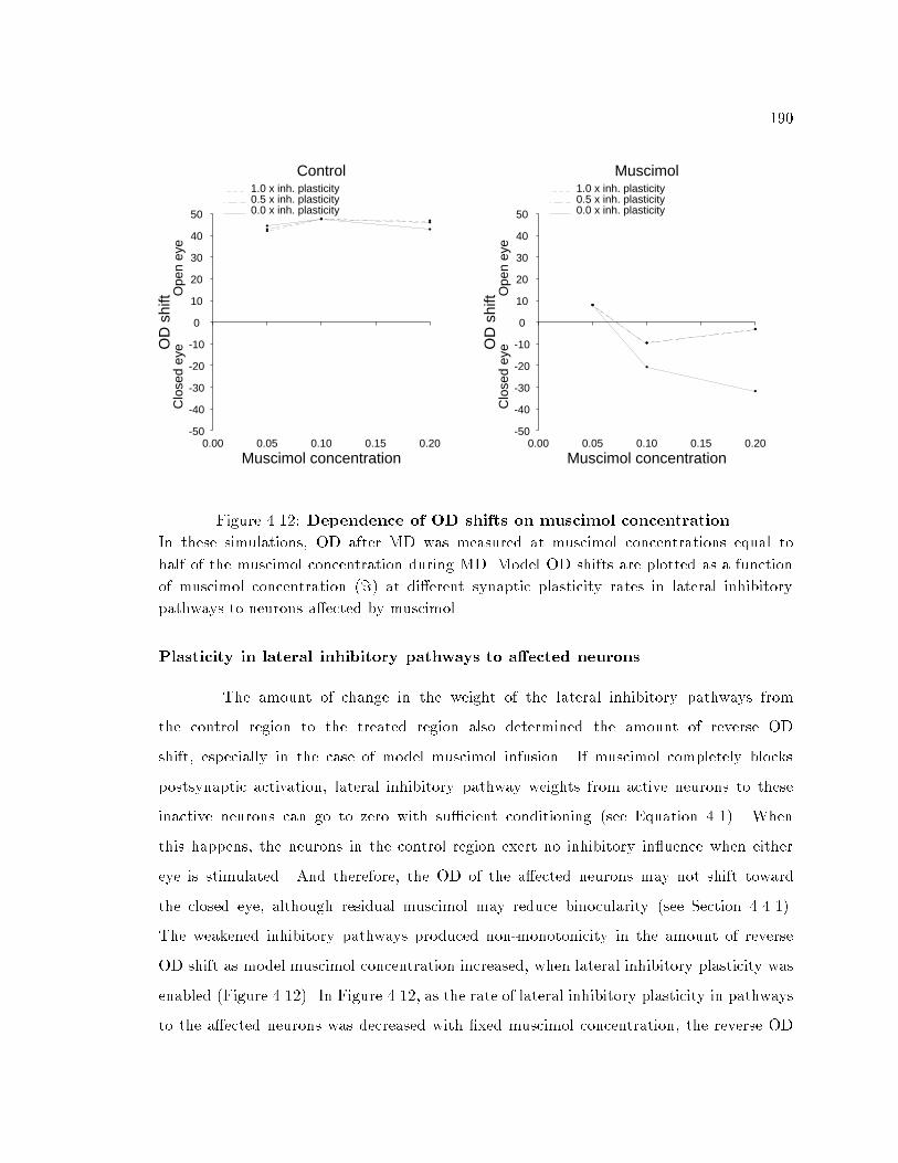
1901.0 x inh. plasticity0.5 x inh. plasticity0.0 x inh. plasticity

-50

-40

-30

-20

-10

0

10

20

30

40

50

0.00 0.05 0.10 0.15 0.20

OD

shi

ft Ope

n ey

eC

lose

d ey

e

Muscimol concentration

Muscimol1.0 x inh. plasticity0.5 x inh. plasticity0.0 x inh. plasticity

-50

-40

-30

-20

-10

0

10

20

30

40

50

0.00 0.05 0.10 0.15 0.20

OD

shi

ft Ope

n ey

eC

lose

d ey

e

Muscimol concentration

Control

Figure 4.12: Dependence of OD shifts on muscimol concentration.In these simulations, OD after MD was measured at muscimol concentrations equal tohalf of the muscimol concentration during MD. Model OD shifts are plotted as a functionof muscimol concentration (=) at di�erent synaptic plasticity rates in lateral inhibitorypathways to neurons a�ected by muscimol.Plasticity in lateral inhibitory pathways to a�ected neuronsThe amount of change in the weight of the lateral inhibitory pathways fromthe control region to the treated region also determined the amount of reverse ODshift, especially in the case of model muscimol infusion. If muscimol completely blockspostsynaptic activation, lateral inhibitory pathway weights from active neurons to theseinactive neurons can go to zero with su�cient conditioning (see Equation 4.1). Whenthis happens, the neurons in the control region exert no inhibitory in uence when eithereye is stimulated. And therefore, the OD of the a�ected neurons may not shift towardthe closed eye, although residual muscimol may reduce binocularity (see Section 4.4.1).The weakened inhibitory pathways produced non-monotonicity in the amount of reverseOD shift as model muscimol concentration increased, when lateral inhibitory plasticity wasenabled (Figure 4.12). In Figure 4.12, as the rate of lateral inhibitory plasticity in pathwaysto the a�ected neurons was decreased with �xed muscimol concentration, the reverse OD

191shift increased. In the case of model APV infusion, this issue is not crucial because theAPV-a�ected neurons remained responsive to input stimulation.In the model, increase in RF width is highly dependent on weakening of lateralinhibitory pathways to the a�ected neurons. The amount of change with �xed NR trainingdepends on the activity of the source neuron and the target neuron (see Equation 4.1).Thus, during NR with APV infusion, if postsynaptic activation is blocked (using APV),lateral inhibitory pathways between a�ected neurons change very little (the only changes arecaused by noise), and neurons show very little RF expansion. At near-normal postsynapticactivation, APV-a�ected neurons do not show much RF expansion because lateral inhibitorypathway strengths remain close to normal levels. At some intermediate, weak postsynapticactivation levels, APV-a�ected neurons show RF expansion (Figure 4.13). The RF widthof neurons a�ected by muscimol during NR is also an inverted-U function of the strength ofmuscimol (Figure 4.13). In Figure 4.13 the RF properties were measured with zero residualAPV or muscimol. Figure 4.13 shows responsiveness and RF width in the presence of APVor muscimol. During APV infusion, the a�erent excitatory plasticity was blocked. A�erentexcitatory plasticity was unchanged during model muscimol infusion.In the EXIN lateral inhibitory plasticity rule (Equation 4.1), the postsynapticactivation determines the stable-state weight of the inhibitory pathways, and thepresynaptic activation determines the rate of weight change. Thus, if the network is trainedfor a su�ciently long time, RF widths will increase as a function of the concentration ofAPV (instead of being an inverted-U curve).During NR with very strong muscimol infusion, noise in the EXIN plasticityrules dominates neuronal activation. When this happens, neurons have no selectivity,and weight changes occur because of noise, resulting in weakening of a�erent excitatoryand lateral inhibitory pathways. When = = 0:8, model cortical neuronal activationswere completely suppressed. After 1,500,000 presentations of binocular inputs, the averagemaximal responsiveness to monocular input was 0:073 (mean)�0:003 (standard deviation),and the average monocular RF width was 1:615� 0:121 (RF width increased).

192InitialAfter 100,000 stepsAfter 200,000 steps

0.0

0.5

1.0

1.5

2.0

0.000 0.225 0.450 0.675 0.900

RF

wid

thAfferent excitation blocking strength of APV

APVInitialAfter 100,000 stepsAfter 200,000 steps

0.0

0.5

1.0

1.5

2.0

0.000 0.225 0.450 0.675 0.900

Neu

rona

l res

pons

iven

ess

X 1

0

Afferent excitation blocking strength of APV

APV

InitialAfter 100,000 stepsAfter 200,000 steps

0.0

0.5

1.0

1.5

2.0

0.000 0.200 0.400

RF

wid

th

Muscimol concentration

MuscimolInitialAfter 100,000 stepsAfter 200,000 steps

0.0

0.5

1.0

1.5

2.0

0.000 0.200 0.400

Neu

rona

l res

pons

iven

ess

X 1

0

Muscimol concentration

Muscimol

Figure 4.13: Dependence of RF width and responsiveness on cortical activation.The model cortical neuronal responsiveness to monocular inputs (left) and monocular RFwidth (right) was measured after NR with infusion of APV (top) and muscimol (bottom)with no residual APV or muscimol. With APV infusion, ! < 1, the learning rate � inEquation 2 was set to zero; i.e., a�erent excitatory plasticity was blocked. APV a�erentexcitation blocking strength was 1� !. During muscimol infusion, � was unchanged.

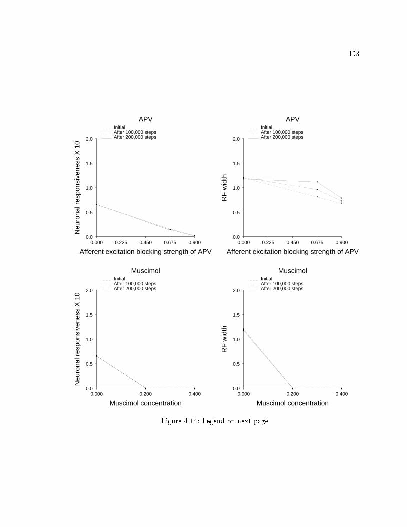
193InitialAfter 100,000 stepsAfter 200,000 steps

0.0

0.5

1.0

1.5

2.0

0.000 0.225 0.450 0.675 0.900

RF

wid

th

Afferent excitation blocking strength of APV

APVInitialAfter 100,000 stepsAfter 200,000 steps

0.0

0.5

1.0

1.5

2.0

0.000 0.225 0.450 0.675 0.900

Neu

rona

l res

pons

iven

ess

X 1

0

Afferent excitation blocking strength of APV

APV

InitialAfter 100,000 stepsAfter 200,000 steps

0.0

0.5

1.0

1.5

2.0

0.000 0.200 0.400

RF

wid

th

Muscimol concentration

MuscimolInitialAfter 100,000 stepsAfter 200,000 steps

0.0

0.5

1.0

1.5

2.0

0.000 0.200 0.400

Neu

rona

l res

pons

iven

ess

X 1

0

Muscimol concentration

Muscimol

Figure 4.14: Legend on next page.

194Figure 4.14: RF width and responsiveness in the presence of APV or muscimol.Figure on previous page. The model cortical neuronal responsiveness to monocular inputs(left) and monocular RF width (right) was measured after NR with infusion of APV(top) and muscimol (bottom). The measurements were made in the presence of APVor muscimol. With APV infusion, as ! was decreased, the learning rate � in Equation 2also was decreased by the same factor. APV a�erent excitation blocking strength is 1� !.During muscimol infusion, � was not changed. The average maximal responsiveness of themodel cortical neurons to binocular inputs used during NR in the presence of APV ormuscimol was 6:546� 10�2 (mean) � 2:280� 10�2 (standard deviation) with ! = 0:325,1:025� 10�2 � 1:467� 10�3 with ! = 0:1, 6:157� 10�2 � 2:055� 10�3 with = = 0:2, and1:283� 10�1 � 9:790� 10�4 with = = 0:4. The normal average maximal responsiveness ofthe model cortical neurons to binocular inputs was 1:893� 10�1 � 9:145� 10�4.4.5 DiscussionThe salient e�ects of the infusion of muscimol or APV during MD are an OD shifttoward the open eye in the control region and a reverse OD shift toward the closed eye.These e�ects have been modeled using the EXIN synaptic plasticity rules (Marshall, 1995).The model is based on the observation that neurons in the control regions become lessresponsive to closed eye stimulation and hence exert less inhibition to neurons in the infusionregion, where a�erent synapses do not change. In addition, the aspeci�c action of APV andmuscimol contributes to changes in cortical properties.In two experiments (Bear et al., 1990; Reiter & Stryker, 1988), OD was measuredwithin 48 hrs of stoppage of infusion, and responsiveness of neurons in the infusion sitecontinued to increase. Bear et al. (1990) showed that responsiveness of neurons in theAPV infusion site three days after stoppage of infusion was greater than the controlresponsiveness. This suggests a relatively long residual e�ect of muscimol and APV.Therefore, a small residual amount of APV or muscimol was assumed during measurementof model cortical properties in the present model.Lateral inhibitory interactions can also play a role in producing reverse OD shiftseven if a covariance rule (Miller et al., 1989; Stanton & Sejnowski, 1989) were used fora�erent excitatory synaptic plasticity, instead of the EXIN a�erent excitatory plasticityrule. The covariance rule would weaken a�erent excitatory pathways from the open eye

195to muscimol or APV treated neurons, thereby producing OD shift toward the closedeye. Furthermore, weakening of a�erent pathways from the closed eye to control neuronsaccording to the covariance rule would cause an additional OD shift toward the closed eyebecause of lateral inhibitory interactions, as in the EXIN model.4.5.1 Loss of cortical neuronal stimulus feature selectivitySeveral cortical properties { orientation selectivity, disparity selectivity, lengthselectivity, spatial frequency selectivity, motion direction selectivity, etc. { may depend onlateral inhibition (Bonds & DeBruyn, 1985; Sillito, 1979; Somers et al., 1995; Somogyi &Martin, 1985). Speci�city of cortical neurons for several stimulus features is abolished bycortical infusion of a GABAA antagonist (Sillito, 1975, 1977, 1979). Blocking intracorticalinhibition also reveals new peripheral regions capable of evoking neuronal responses(Lane et al., 1997; Sillito et al., 1981).Kasamatsu et al. (1998a) observed loss of orientation selectivity and directionselectivity after APV infusion in adult cat primary visual cortex. Bear et al. (1990) reportedloss of orientation selectivity in a region a�ected by APV after MD with APV infusion.Prolonged binocular deprivation reduces neuronal responsiveness and orientation selectivity(Fr�egnac & Imbert, 1984). In these experiments, cortical activation was much lower thanduring normal rearing.According to the EXIN lateral inhibitory plasticity rule, weak neuronal activationis su�cient for weakening lateral inhibitory pathways between these neurons (albeitrelatively slowly) and may lead to reduction of neuronal stimulus feature speci�city.During chronic binocular deprivation, the a�erent pathways may weaken, thereby weakeningneuronal responsiveness. In the model, loss of position selectivity (increase in RF width)occurred after APV infusion and after MD with APV infusion.Biologically, the EXIN inhibitory rule could be realized either by modifying theweights of inhibitory synapses onto excitatory neurons or by modifying the weights ofexcitatory synapses onto inhibitory interneurons. In the developing cortex, lateral excitatorypathways too may undergo synaptic plasticity. If changes in the lateral inhibitory pathwaysdominate changes in lateral excitatory pathways, the e�ects predicted by the EXIN model

196would arise.The loss of orientation selectivity during APV infusion observed byKasamatsu et al. (1998a) could also be caused by weakening of a�erent excitatory inputsto inhibitory neurons, thus reducing intracortical inhibition. Kasamatsu et al. (1998a)observed reduced orientation selectivity and binocularity during APV infusion. In theEXIN model, model APV infusion in a group of neurons caused RF expansion in somecontrol neurons. When lateral inhibitory plasticity was enabled, APV-a�ected neuronsrecovered binocularity. Thus, the model suggests both an immediate and a prolonged e�ectof APV on neuronal selectivity. The model suggests that APV-a�ected neurons will haveweak orientation selectivity after complete removal of APV because of weakened lateralinhibitory pathways.The loss of stimulus feature speci�city of cortical neurons based on theEXIN rule is valid even if lateral excitatory pathways contribute to feature selectivity(Somers et al., 1995). Somers et al. (1995) assume that lateral excitation from neighboringneurons is orientation selective, and weakened lateral inhibition will render all neurons lessselective.4.5.2 Model predictionsIn the model, it was assumed that plasticity in lateral inhibitory pathways is nota�ected by muscimol or APV. However, in the cortex it is possible that APV blocks plasticityin lateral excitatory pathways to inhibitory neurons; and if the biological realization of theEXIN lateral inhibitory rule requires plasticity in lateral excitatory pathways to inhibitoryneurons, then APV can a�ect plasticity in lateral inhibitory pathways in the cortex. Thereare very few reports of possible plasticity in lateral inhibitory pathways (e.g., Miles &Wong, 1987). The e�ect of muscimol on plasticity in lateral inhibitory pathways is notknown. Thus, the e�ects produced by the lateral inhibitory rule in the simulations arepredictive.

197Intracellular measurement of excitatory and inhibitory postsynaptic potentialsThalamocortical stimulation produces monosynaptic excitatory postsynapticpotentials (EPSPs) and disynaptic inhibitory postsynaptic potentials (IPSPs) (Gil &Amitai, 1996; Ferster, 1989). The EXIN model makes the following predictions, foryoung animals during their critical period after MD with strong concentrations of APVor muscimol.1. Monosynaptic EPSPs evoked in APV or muscimol treated neurons by left or righteye selective thalamocortical a�erent stimulation remain unchanged. (It should beensured that there is no residual APV or muscimol.)2. Monosynaptic EPSPs evoked in control neurons by closed eye selective thalamocorticala�erent stimulation decrease substantially, and monosynaptic EPSPs evoked in controlneurons by open eye selective thalamocortical a�erent stimulation may increaseslightly (see Section 4.2.3).3. Disynaptic IPSPs in neurons treated with muscimol or APV by stimulation ofthalamocortical a�erents selective to the closed eye decreases, because neurons inthe control region become weakly responsive to closed eye stimulation and hence sendweaker inhibition to neurons a�ected by muscimol or APV.4. Disynaptic IPSPs in control neurons caused by stimulation of thalamocortical a�erentsselective to either eye may change by a small amount (the a�erent excitatory pathwaysto these neurons strengthen slightly because of increased correlation with monocularinputs, and lateral inhibitory pathways to these neurons weaken by a small amountbecause the neurons are weakly active).In contrast, models based on depression in the a�erent excitatory pathways fromthe open eye to neurons a�ected by APV or muscimol (Bear et al., 1990; Miller et al., 1989;Reiter & Stryker, 1988) predict decrease in monosynaptic EPSPs in APV or muscimoltreated neurons by stimulation of open eye selective thalamocortical a�erents.

198Changes in RF width and stimulus feature selectivity as a function of corticalactivity During binocular rearing of young animals for a �xed duration within their criticalperiod, neuronal activation of a small region of the cortex can be varied, e.g., by infusionof muscimol or APV, or by controlling the input stimulation strength. The EXIN modelsuggests the following predictions.1. With muscimol or APV infusion, the amount of increase in RF size andneuronal responsiveness and the amount of decrease in stimulus feature selectivity(e.g., orientation selectivity) as a function of cortical activation level (concentration ofmuscimol or APV) will be an inverted-U shaped curve (see Section 4.4.3, Plasticity inlateral inhibitory pathways to a�ected neurons). Because of normal input stimulation,the a�erent excitatory pathways may not change during muscimol infusion.2. As the strength of input stimulation is decreased (cortical activation also decreases),the magnitude of change in RF size, responsiveness, and stimulus feature selectivitywill be inverted-U shaped. When input stimulation strength is decreased, the a�erentexcitatory pathways may weaken; therefore, the change in RF width, neuronalresponsiveness, and stimulus feature selectivity will depend on whether decreasein excitation or decrease in inhibition dominates. During prolonged binoculardeprivation, neuronal responsiveness and orientation selectivity decrease (Fr�egnac &Imbert, 1984).3. APV can be infused to block a�erent excitatory plasticity when the strength ofinput stimulation is decreased. The amount of increase in RF size and neuronalresponsiveness and the amount of decrease in stimulus feature selectivity will beinverted-U shaped as a function of the input stimulation strength.Arti�cial scotoma conditioning with pharmacological treatmentsPettet and Gilbert (1992) showed RF expansion in primary visual cortical neuronswhose RF was occluded with just 15 minutes of arti�cial scotoma conditioning in one

199eye with the other eye closed. This RF expansion has been modeled by weakeninglateral inhibitory pathways from active neurons to inactive neurons, without requiring anyplasticity in the a�erent excitatory pathways (Kalarickal & Marshall, 1997; Marshall &Kalarickal, 1997). The reduced weights of inhibitory pathways to neurons whose RF is insidethe scotoma from neurons whose RF is outside then allows greater and wider responses bythe neurons whose RF is inside. In contrast, Sirosh et al. (1996) modeled the RF expansionusing a�erent excitatory plasticity. During arti�cial scotoma conditioning, neurons whoseRF straddles the scotoma boundary have active a�erent excitatory pathways from positionsoutside the scotoma and inactive a�erent excitatory pathways from positions inside thescotoma. Thus, active a�erent excitatory pathways to the neuron can be competitivelyweakened. Since a�erent excitatory plasticity in animals during the critical period is easilyinduced (Hubel & Wiesel, 1965, 1970; Hubel et al., 1977), arti�cial scotoma conditioningwith cortical infusion of APV can be used to assess (1) the e�ciency of APV in blockinga�erent plasticity and (2) the contribution of a�erent excitatory and lateral inhibitoryplasticity in producing the e�ects of arti�cial scotoma conditioning.We propose the following experiments:1. Perform arti�cial scotoma conditioning in animals during the critical period. Withboth a�erent and lateral inhibitory synaptic plasticity, the EXIN model predicts(a) RF expansion in neurons whose RF is in the scotoma region during arti�cialscotoma conditioning; and(b) RF contraction in neurons whose RF straddles the arti�cial scotoma boundary.These neurons will be active during conditioning, and hence the a�erentexcitatory pathways from parts of the scotoma region will weaken (Kalarickal &Marshall, 1997; Sirosh et al., 1996).2. Perform arti�cial scotoma conditioning with a large cortical infusion of APV. If APVblocks a�erent excitatory plasticity, the EXIN model predicts(a) RF expansion in neurons whose RF is in the scotoma region (because of lateralinhibitory plasticity); and

200(b) no RF contraction in neurons whose RF straddles the scotoma boundary.Temporary cortical scotoma conditioning with normal input stimulationTo determine the role of lateral inhibitory plasticity, a temporary local corticalscotoma can be produced by infusion of muscimol, during normal stimulation in animalsduring their critical period. The EXIN model predicts RF expansion in neurons a�ected bymuscimol (after su�cient time to allow dissipation of the e�ects of muscimol) because ofweakening of lateral inhibitory pathways from the active neurons to the muscimol-treatedinactive neurons. The lateral inhibitory pathways from the muscimol-treated inactiveneurons to other neurons and the a�erent excitatory pathways to the muscimol-treatedneurons may change by a very small amount because of noise. In contrast, if the activea�erent excitatory pathways to the cortical neurons whose activation is suppressed bymuscimol were weakened as proposed by Reiter and Stryker (1988) and Miller et al. (1989),then the RF size of the muscimol-treated neurons would shrink.4.5.3 ConclusionsIn the EXIN model, plasticity in lateral inhibitory pathways develops as a functionof overlap in the RF of neurons. Previously, it was shown that lateral inhibitory plasticityproduces neurons with high selectivity and sparse distributed coding (Marshall, 1995;Marshall & Gupta, 1998). Therefore, the role of the lateral inhibitory plasticity rule inproducing RF changes was studied in detail in the context of MD with infusion of APV andmuscimol. The predictions made based on the EXIN plasticity rules can be used to designexperiments to reveal the rules of a�erent excitatory and lateral inhibitory plasticity andtheir role in cortical plasticity.

Chapter 5Models of receptive �eld dynamicsin visual cortexAbstractThe position, size, and shape of the receptive �eld (RF) of some cortical neuronschange dynamically, in response to arti�cial scotoma conditioning (Pettet & Gilbert, 1992)and to retinal lesions (Chino et al., 1992; Darian-Smith & Gilbert, 1995) in adult animals.The RF dynamics are of interest because they show how visual systems may adaptivelyovercome damage (from lesions, scotomas, or other failures), may enhance processinge�ciency by altering RF coverage in response to visual demand, and may perform perceptuallearning. This chapter presents an a�erent excitatory synaptic plasticity rule and a lateralinhibitory synaptic plasticity rule { the EXIN rules (Marshall, 1995a) { to model persistentRF changes after arti�cial scotoma conditioning and retinal lesions. The EXIN modelis compared to the LISSOM model (Sirosh et al., 1996) and to a neuronal adaptationmodel (Xing & Gerstein, 1994). The rules within each model are isolated and areanalyzed independently, to elucidate their roles in adult cortical RF dynamics. Basedon computer simulations, the EXIN lateral inhibitory synaptic plasticity rule and the

202LISSOM lateral excitatory synaptic plasticity rule produced the best �t with currentneurophysiological data on visual cortical plasticity in adult animals (Chino et al., 1992;Darian-Smith & Gilbert, 1995; Pettet & Gilbert, 1992) including (1) the retinal position ofthe expanding RFs, (2) the amount of change in spontaneous activation in the absence of anyvisual stimulation, (3) the corticotopic direction in which responsiveness returns to lesionedcortex, (4) the direction of RF shifts, (5) the amount of change in response to blank stimuli,and (6) the lack of dynamic RF changes during conditioning with a retinal lesion in oneeye and the unlesioned eye kept open, in adult animals. The e�ects of the LISSOM lateralinhibitory synaptic plasticity rule during arti�cial scotoma conditioning are in con ict withthose of the other two LISSOM synaptic plasticity rules. A novel \complementary scotoma"conditioning experiment, in which stimulation of two complementary regions of visual spacealternates repeatedly, is proposed to di�erentiate the predictions of the EXIN and LISSOMrules.5.1 IntroductionIn experiments using arti�cial scotoma conditioning (Pettet & Gilbert, 1992)and retinal lesions (Chino et al., 1992; Darian-Smith & Gilbert, 1995), neurons inprimary visual cortex corresponding to a particular region of visual space were deprivedof visual stimulation, while neurons corresponding to a surrounding region received visualstimulation. In response to these manipulations, a variety of dynamic changes occurred inthe position, size, and shape of the receptive �eld (RF) of some of the neurons. For example,after 15 minutes of arti�cial scotoma conditioning, the RF area of some cortical neuronswhose RF was located inside the scotoma expanded by a factor of �ve; after 15 minutes ofsubsequent normal stimulation, the RF returned to its original size (Pettet & Gilbert, 1992).The dynamic RF expansion following arti�cial scotoma conditioning in one eye also transfersto the other eye (Volchan & Gilbert, 1994).Pettet and Gilbert (1992) simulated a retinal lesion experiment by presenting apattern of moving lines in the visual �eld while masking out an arti�cial \scotoma" regioncovering the original RF of the recorded neuron. After 10{15 minutes of stimulation, a

203�ve-fold average expansion in RF area was found. In the second phase of the experiment,the scotoma region was unmasked, and moving lines were presented in the whole �eld. Afterseveral minutes of stimulation, the RF shrank back to its original extent. The RF expansionand contraction was repeatable. A key observation was that stimulation exclusively in thesurrounding region was necessary for the RF expansion to occur. Exposure to a blankscreen for as long as 20 minutes had little e�ect on the RF size.Pettet and Gilbert (1992) tested the e�ect of orientation of the conditioning stimulion RF expansion, during arti�cial scotoma conditioning. For a few neurons (3 out of 15),they found an expansion with iso-orientation conditioning stimuli and did not �nd anexpansion with the orthogonal pattern. In these cases, the orthogonal pattern actuallyreduced the RF size and responsiveness of the neuron.Darian-Smith and Gilbert (1995) studied topographic reorganization in the striatecortex of the adult cat and monkey after binocular retinal lesions, using physiological andanatomical techniques. They found that immediately (between 5 minutes and up to 1 hour)after making corresponding retinal lesions of 3:5�{14� in diameter, there was a corticalscotoma region containing neurons whose RF was located more than 0.5{1.0 mm insidethe initial scotoma boundary. However, cortical neurons located close to or just insidethe cortical scotoma boundary showed an increase in RF size. The greatest expansionoccurred for neurons whose RF was located closest to the scotoma boundary. In addition,the expanded RFs shifted centrifugally toward the outside of the scotoma. Neurons thatacquired responsiveness to locations outside the scotoma, i.e., neurons in the recoveredregion of the original cortical scotoma, were less responsive, more sluggish in their response,and more easily fatigued compared to those in normal cortex or in cortex located more than1 mm outside the cortical scotoma boundary. In spite of the changes in their RF size andposition, these neurons retained some of their original RF properties, such as directionality,orientation speci�city, and binocularity.Measurements within the same cortex 2{12 months after the lesions showedthat cortical neurons located several millimeters inside the original boundary of thecortical scotoma became responsive to stimulation of perilesion retina (Darian-Smith &Gilbert, 1995). Over time, function returned to the cortex in a roughly concentric inward

204direction. The cortical reorganization was accompanied by RF shifts. In spite of distortionsin representation, topographic order was maintained.In contrast to the cortical reorganization, the LGN scotoma and thalamocorticala�erents did not undergo any change, as re ected in electrophysiological recordings andanatomical studies. This led Darian-Smith and Gilbert to conclude that the reorganizationof cortical topography following retinal lesions originates in the cortex and is likely to bemediated, at least in part, by the long-range collaterals of cortical neurons rather than bythalamocortical a�erents.5.1.1 Signi�cance of RF dynamicsThe dynamics of RFs are of interest for several reasons. They reveal someof the ways in which visual systems may adaptively overcome damage from lesionsor scotomas. In addition, they reveal some of the functional organization of visualcortex (Das, 1997; Gilbert, 1998). Dynamic visual RFs might also be related to thedynamic response properties found in other cortical areas (Das, 1997), such as thetactile RF expansion/contraction found in adult somatosensory cortex in response tointracortical microstimulation (Recanzone et al., 1992b) and localized peripheral stimulation(Recanzone et al., 1992d).Arti�cial scotoma conditioning can elucidate the neural basis of perceptual learning.In perceptual learning, human observers improve their performance in perceptual taskssuch as orientation perception (Fiorentini & Berardi, 1980), vernier acuity (Fahle &Edelman, 1993), and discrimination of texture (Karni & Sagi, 1991) after training (repeatedperformance of a perceptual task). Perceptual learning is stable: it does not wear o� afterperiods without visual stimulation. Furthermore, in these studies perceptual learning wasnot simply a matter of becoming accustomed to the perceptual task. Perceptual learningwas speci�c for features of the training stimuli (Crist et al., 1997; Fahle, 1997); it wasusually con�ned to the portion of the retina that was stimulated during training, or theimprovement was restricted to the orientation of the training stimuli. Since neurons in thevisual cortex are selective for speci�c stimulus features, repeated presentation of trainingstimuli repeatedly activates a small group of neurons. Thus, perceptual learning may be

205realized by cortical plasticity that depends on repeated activation of a group of neurons.In arti�cial scotoma conditioning, visual cortical neurons selective for a particular regionof visual space are deprived of visual stimulation while neurons selective for surroundingvisual space receive stimulation. Thus, arti�cial scotoma conditioning provides a systematicprocedure to control the activation of speci�c groups of neurons and to study the neuralbasis of perceptual learning.5.1.2 Modeling of RF dynamicsFigure 5.1 shows the input pathways to primary visual cortical neurons. The RFof a cortical neuron can be a�ected by changes in the inputs to the neuron. The long-range horizontal excitatory or inhibitory pathways in visual cortex have been regarded asthe substrate for RF dynamics (Darian-Smith & Gilbert, 1995; Das & Gilbert, 1995ab;Gilbert et al., 1996; Pettet & Gilbert, 1992; Somogyi & Martin, 1985; Volchan &Gilbert, 1994). It has been shown that dynamic RF changes result from changes in theamount of excitation and/or inhibition received by the neurons (Chapman & Stone, 1996;Petersen & Taylor, 1997). Changes in the amount of excitation and/or inhibition to neuronscan result from neuronal adaptation (DeAngelis et al., 1995; Xing & Gerstein, 1994),short-term inhibitory synaptic adaptation (Todorov et al., 1997), long-term synapticmodi�cations in long-range horizontal pathways (Darian-Smith & Gilbert, 1994, 1995;Das & Gilbert, 1995ab; Gilbert et al., 1996; Pettet & Gilbert, 1992), long-term synapticplasticity in lateral inhibitory pathways (Marshall & Kalarickal, 1997), or long-term synapticplasticity in a�erent excitatory pathways (Marshall, 1995a; Sirosh et al., 1996). Rea�erentfeedback pathways between cortical layers may also be involved in producing corticalplasticity (Gilbert, 1996).A drawback of adaptation-based models (Todorov et al., 1997; Xing &Gerstein, 1994) is that they cannot sustain the RF expansions during periods with no visualstimulation in arti�cial scotoma conditioning as reported by Pettet and Gilbert (1992).Sirosh et al. (1996) attributed RF expansion after arti�cial scotoma conditioning to a�erentexcitatory plasticity in their LISSOM model. Their model also had plasticity in lateralexcitatory and lateral inhibitory pathways, but the role of these forms of plasticity in

206

AAAAAAAAAAAAAAAAAAAAAAAAAAAAAAAAAAAAAAAAAAAAAAAAAAAAAAAAAAAAAAAAAAAAAAAAAAAAAAAAAAAAAAAAAAAAAAAAAAAAAAAAAAAAAAAAAAAAAAAAAAAAAAAAAAAAAAAAAAAAAAAAAAAAAAAAAAAAAAAAAAAAAAAAAAAAAAAAAAAAAAAAAAAAAAAAAAAAAAAAAAAAAAAAAAAAAAAAAAAAAAAAAAAAAAAAAAAAAAAAAAAAAAAAAAAAAAAAAAAAAAAAAAAAAAAAAAAAAAAAAAAAAAAAAAAAAAAAAAAAAAAAAAAAAAAAAAAAAAAAAAAAAAAAAAAAAAAAAAAAAAAAAAAAAA

AAAAAAAAAAAAAAAAAAAAAAAAAAAAAAAAAAAAAAAAAAAAAAAAAAAAAAAAAAAAAAAAAAAAAAAAAAAAAAAAAAAAAAAAAAAAAAAAAAAAAAAAAAAAAAAAAAAAAAAAAAAAAAAAAAAAAAAAAAAAAAAAAAAAAAAAAAAAAAAAAAAAAAAAAAAAAAAAAAAAAAAAAAAAAAAAAAAAAAAAAAAAAAAAAAAAAAAAAAAAAAAAAAAAAAAAAAAAAAAAAAAAAAAAAAAAAAAAAAAAAAAAAAAAAAAAAAAAAAAAAAAAAAAAAAAAAAAAAAAAAAAAAAAAAAAAAAAAAAAAAAAAAAAAAAAAAAAAAAAAAAAAAAAAAA

LGN

Layers II-IV+

++

+++

+ +

+ ++ +

Feedbackexcitatorypathways

Afferentexcitatorypathways + +

+++ Lateral

inhibitorypathways

Lateralexcitatorypathways

AAAAAAAAAAAAAAAAAAAAAAAAAAAAAAAAAAAAAAAAAAAAAAAAAAAAAAAAAAAAAAAAAAAAAAAAAAAAAAAAAAAAAAAAAAAAAAAAAAAAAAAAAAAAAAAAAAAAAAAAAAAAAAAAAAAAAAAAAAAAAAAAAAAAAAAAAAAAAAAAAAAAAAAAAAAAAAAAAAAAAAAAAAAAAAAAAAAAAAAAAAAAAAAAAAAAAAAAAAAAAAAAAAAAAAAAAAAAAAAAAAAAAAAAAAAAAAAAAAAAAAAAAAAAAAAAAAAAAAAAAAAAAAAAAAAAAAAAAAAAAAAAAAAAAAAAAAAAAAAAAAAAAAAAAAAAAAAAAAAAAAAAAAAAAA

+

Layer VI /higher cortical areas

inhibitory neuron

excitatory neuron

Figure 5.1: Site of RF changes.The RF of cortical neurons changes when input excitation and inhibition to the neuronschange. Cortical neurons receive a�erent, lateral, and feedback excitation. Cortical neuronsreceive lateral inhibition from inhibitory neurons (shown by the shaded ellipse in layer 2).The excitatory cortical neurons (represented by the un�lled ellipses) send lateral excitationto excitatory and inhibitory neurons. Changes in input excitation and inhibition can occurbecause of synaptic plasticity in excitatory and inhibitory synapses, respectively, or becauseof adaptation cortical neurons.

207RF changes after arti�cial scotoma conditioning was not analyzed.This chapter compares the properties of RF changes produced by several modelsof cortical plasticity to the neurobiological data on RF changes after arti�cial scotomaconditioning and after retinal lesions in adult animals. In particular, RF changesafter arti�cial scotoma conditioning and retinal lesions produced by the EXIN rules(Marshall, 1990a, 1995a), the LISSOM rules (Sirosh & Miikkulainen, 1994ab, 1995, 1997;Sirosh et al., 1996), and an adaptation rule (Xing & Gerstein, 1994) are analyzed.EXIN plasticity rulesThe EXIN model uses an an instar Hebbian a�erent excitatory synaptic plasticityrule and an outstar anti-Hebbian lateral inhibitory synaptic plasticity rule (Marshall, 1990a,1995a). An instar rule is enabled when the postsynaptic neuron is activated, and excitatorypathways into the neuron undergo synaptic plasticity (Grossberg, 1972, 1976ab), whereasan outstar rule is enabled when the presynaptic neuron or presynaptic element is activated,and excitatory pathways out of the neuron or the presynaptic element undergo synapticplasticity (Grossberg, 1976c). This subtle distinction makes dramatic di�erence in theplasticity and behavior of the neural circuits (Grossberg, 1976abc; Marshall, 1995a).In EXIN networks, the instar excitatory synaptic plasticity rule modi�es theweights of a�erent excitatory pathways to active neurons so that the active neuronsbecome more responsive to the currently presented input pattern. The instar excitatorysynaptic plasticity rule is responsible for the development of the broad excitatory RF of theneurons. The development of weights of lateral inhibitory pathways according to the outstarlateral inhibitory synaptic plasticity rule ensures that di�erent neurons become selective todi�erent input patterns. Yet, if the input environment contains several similar patterns, theoutstar lateral inhibitory synaptic plasticity rule causes strong lateral inhibitory pathwaysto develop between neurons selective for the similar input patterns, thereby producing highdiscrimination. In EXIN networks, lateral inhibitory pathways from often-activated neuronsto unresponsive neurons weaken, thereby making the unresponsive neurons more likely torespond to some input. The outstar lateral inhibitory synaptic plasticity rule is responsiblefor dispersion of neuronal selectivity and sharpening of the RF of the neurons. The EXIN

208rules develop e�cient representation of input patterns according to their distribution in aninput environment. The EXIN rules self-organize networks capable of representing multiplesuperimposed patterns, ambiguous patterns, overlapping patterns at di�erent scales, andcontextually constrained patterns starting from completely nonspeci�c a�erent excitatoryand lateral inhibitory pathway weights (Marshall, 1995a).LISSOM plasticity rulesThe LISSOM model (Sirosh & Miikkulainen, 1994b) uses instar Hebbian a�erentexcitatory and lateral excitatory synaptic plasticity rules, and an instar anti-Hebbianlateral inhibitory synaptic plasticity rule. Unlike the EXIN model, the LISSOM modelhas modi�able lateral excitatory pathways and uses an instar lateral inhibitory synapticplasticity rule. However, like the EXIN rules, the LISSOM rules produce a sparse,distributed coding that reduces redundancies (Marshall, 1995a; Marshall & Gupta, 1998;Sirosh et al., 1996). Lateral excitatory pathways in the LISSOM model help the developmentof a topographic RF arrangement. The LISSOM lateral excitatory and inhibitory synapticplasticity rules cause highly speci�c lateral pathway connectivity to develop between neuronsthat have similar RF properties (Sirosh & Miikkulainen, 1997).Adaptation rulesIn adaptation models (Xing & Gerstein, 1994), the RF changes occur as a resultof adaptive modi�cations in the sensitivity of single neurons, rather than as a result ofmodi�cations in the synaptic weights between pairs of neurons.5.1.3 Signi�cance and contributions of this chapterThis chapter analyzes the role of each rule individually. The EXIN rules and theLISSOM rules have been used to model development of cortical properties and functions inyoung animals. Studies on young animals in their critical periods show that the a�erent andlateral pathway connectivity in the primary visual cortex are modi�ed by changes in thevisual environment (Hubel & Wiesel, 1965, 1970; Hubel et al., 1977; Katz & Callaway, 1992).However, the neural basis of adult cortical plasticity, e.g., RF changes after arti�cial scotoma

209conditioning and retinal lesions in adult animals, is not known. Thus, the rules in theEXIN model, the LISSOM model, and the adaptation models are studied individuallyto determine whether they produce e�ects consistent with the experimentally observedRF changes after arti�cial scotoma conditioning and retinal lesions in adult animals. Thepossible e�ects of the full EXIN and the full LISSOM model are also discussed. Thesimulation results based on individual rules serve as predictions for the e�ects of arti�cialscotoma conditioning and retinal lesions in adult animals in the presence of pharmacologicalagents that block plasticity in speci�c pathways, e.g., NMDA receptor antagonists whichblock plasticity in excitatory pathways (Kirkwood et al., 1993). The simulations showdi�erences in two plausible rules for plasticity in lateral inhibitory pathways (the outstarEXIN lateral inhibitory rule and the instar LISSOM lateral inhibitory rule) in the contextof arti�cial scotoma conditioning and retinal lesions. A novel experiment is suggested tofurther di�erentiate between the rules.In this chapter, experimental data on cortical e�ects of arti�cial scotomaconditioning and retinal lesions are used to constrain plausible rules for dynamic RF changes.In particular,1. the chapter analyzes the e�ects of an instar and an outstar lateral inhibitory synapticplasticity rule during scotoma conditioning;2. the e�ects of di�erent plausible ways of modifying e�ective inhibition to neuronsduring scotoma conditioning, e.g. due to changes in lateral excitatory or a�erentexcitatory pathway strength, or neuronal adaptation, are studied;3. some of the possible rules that could produce dynamic RF changes are eliminatedbased on comparison with experimental data;4. the chapter shows that the EXIN outstar lateral inhibitory synaptic plasticity rule andthe LISSOM instar lateral excitatory synaptic plasticity rule are su�cient to accountfor most of the data on arti�cial scotoma conditioning and on the short-term e�ects ofretinal lesions (the e�ects of orientation selectivity on RF dynamics during arti�cialscotoma were not simulated);

2105. the su�ciency of the EXIN lateral inhibitory synaptic plasticity rule in producingRF changes after arti�cial scotoma conditioning and after retinal lesions in adultanimals provides indirect evidence for the existence of plasticity in lateral inhibitorypathways and predicts characteristics of inhibitory synaptic plasticity in cortex; and6. a novel experiment, complementary scotoma conditioning, is proposed to distinguishthe e�ects caused by neuronal adaptation from those caused by synaptic plasticity.5.2 Methods5.2.1 Network simulation organizationThe architecture used for the simulations is a two-layered neural network witha�erent and lateral connections, corresponding to parts of subcortex and primary visualcortex. A patch of neurons in the primary visual cortex, arranged in a 30 � 30 grid ofspatial positions, was simulated. The position of each neuron's RF corresponded to theneuron's position in the grid. Adjacent RFs initially had more than 50% spatial overlap.In the computer simulations, Layer 1 (corresponding to LGN processing) andLayer 2 (corresponding to early laminae of primary visual cortex) each had a 30� 30 arrayof neurons. For ease of simulation, the initial a�erent pathway weight and lateral pathwayweight distributions in the simulations are chosen to be spatially isotropic. Furthermore,the input feature to these networks is an isotropic Gaussian blob (see Section 5.2.2), whichwhen used to train the networks produces spatially isotropic receptive �elds. However,isotropic RFs are not essential for these networks to produce changes in RF propertiesduring the various forms of input conditioning. The EXIN and LISSOM learning rules arecompetitive learning rules and produce orientation selective neurons if the input featuresare oriented (Marshall, 1990d; Sirosh et al., 1996); scotoma conditioning using orientedfeatures would a�ect the networks as described in Sections 5.2.5 and 5.2.6. The adaptationnetworks are based on neuronal adaptation, without synaptic plasticity. The weightsin the adaptation networks can be assigned to produce orientation selective neurons.The adaptation of the orientation selective neurons during arti�cial scotoma conditioning

211will produce RF expansions because of di�erences in adaptation levels as explained inSection 5.2.7.Following Xing and Gerstein (1994), orientation selectivity is not built into thesimulations. This is a gross simpli�cation, as it discounts the e�ects of neurons selectiveto other orientations on dynamic RF changes. The simpli�cation of representing onlyiso-orientation selective neurons in Layer 2 is partially justi�ed by observing that theRF expansion was more pronounced and robust during conditioning with iso-orientationpatterns than during conditioning with ortho-orientation patterns (Pettet & Gilbert, 1992).In the discussion section, a mechanism for orientation selectivity is described which maymodel the in uence of neurons with other orientation selectivity on dynamic RF properties.The following symbols are used to refer to the various entities of the network.The indices (i; j) and (k; l) are used to refer to Layer 1 neurons, and (p; q), (r; s), and(u; v) refer to Layer 2 neurons, where i; j; k; l; p; q; r; s; u; v 2 f�15; : : : ; 14g. These indicesalso represent the retinotopic coordinates of the neurons' RF. The weight of the a�erentexcitatory connection pathway from a Layer 1 neuron (i; j) to a Layer 2 neuron (p; q) isdenoted by Z+ij;pq(t). The weight of the lateral inhibitory connection pathway and the weightof the lateral excitatory connection pathway from Layer 2 neuron (p; q) to Layer 2 neuron(r; s) are represented by Z�pq;rs(t) and Z+pq;rs(t), respectively. These pathway weight valuesmay represent the e�ect of a monosynaptic connection, the total e�ect of a polysynapticchain of connections (see Section 5.5.7), or the population e�ect of multiple direct synapses.The activation levels (mean spike rate) over time of Layer 1 neuron (i; j) and Layer 2 neuron(p; q) are represented by xij(t) and xpq(t), respectively.5.2.2 The inputsThe inputs to Layer 1 were obtained as follows. First, two-dimensional 30 � 30images were convolved with a Gaussian kernel, K, with toroidal wraparound. The inputstimulus at each position in the images could be 0 or 1. The input at each position tookvalue 1 with probability � during a given simulation step. After convolution, the resultantimage was normalized by the maximum intensity value in the image. In the simulations, themean of the normalization factor was 1:68, with a standard deviation of 0:34, over 10,000

212inputs. The resultant images from the normalization stage were the inputs to Layer 1.These inputs to Layer 1 are called normal stimuli.In arti�cial scotoma conditioning, random stimulation in the whole visual �eldexcept in a masked region was followed by whole-�eld random stimulation. To simulateinputs with a scotoma, images with a scotoma were convolved with the kernel K and thennormalized. Input stimuli at positions outside the scotoma region had probability � of beingassigned value 1, and input stimuli inside the scotoma region had value 0. These inputsare called scotoma stimuli. The term \cortical scotoma" refers to the silenced region inLayer 2 as a result of using retinal scotoma stimuli (Xing & Gerstein, 1994; Darian-Smith &Gilbert, 1995).5.2.3 Simulation procedureIn the simulations, the experimental paradigm of Pettet and Gilbert (1992) wasfollowed. The original RF was determined after a period of random whole-�eld stimulation.In all the simulations, the initial whole-�eld stimulation was continued until the sumof the magnitude of individual weight changes after 100 training steps had reached anasymptote. Then the RF was again measured after conditioning with the arti�cial scotoma.To determine reversibility of RF changes, the RF was measured again after whole-�eldstimulation.5.2.4 RF measurementsThe RF was mapped using single-point stimulation, blurred with the Gaussiankernel K, at all input positions (i; j). The RF of a Layer 2 neuron (p; q) is de�ned as thecollection of positions (i; j) at which the test input causes the activation level xpq to exceeda threshold �.5.2.5 The EXIN modelThe EXIN model (Figure 5.2) combines an instar a�erent EXcitatory synapticplasticity rule and an outstar lateral INhibitory synaptic plasticity rule. The EXIN synaptic

213plasticity rules change the weights as a function of the input stimuli so that di�erentneurons become selective for di�erent input patterns and every input pattern is representedby a sparse output pattern (Marshall, 1995a). In scotoma conditioning, a subset of thevisual input is removed, and therefore neurons previously selective for these inputs are notstimulated. The EXIN rules change the weights so that the unstimulated neurons becomeresponsive to di�erent input patterns, resulting in changes in their RFs.The EXIN lateral inhibitory synaptic plasticity ruleThe lateral inhibitory weights, Z�pq;rs, are modi�ed according to the anti-Hebbianrule ddtZ�pq;rs = � G(xpq) ��Z�pq;rs + Q(xrs)� (5.1)(Marshall, 1995a), where � > 0 is a small learning rate constant and G and Q arehalf-recti�ed non-decreasing functions. Thus, whenever a neuron is active, its outputinhibitory connections to other active neurons tend to become slightly stronger (i.e., moreinhibitory), while its output inhibitory connections to inactive neurons tend to becomeslightly weaker . Neuron activations remain within [�C;B] according to a shunting equation(Equation 5.3) based on the Hodgkin model (Hodgkin, 1964); this causes the weight values toremain bounded as well, because according to Equation 5.1, Z�pq;rs(t) 2 [0;Q(B)] for t � 0,if Z�pq;rs(0) 2 [0;Q(B)] (Grossberg, 1982). The weight change in Equation 5.1 approacheszero as Z�pq;rs approaches Q(xrs), the weight change is positive when Z�pq;rs < Q(xrs), andthe weight change is negative when Z�pq;rs > Q(xrs). The weight change approaches zero asZpq;rs approaches Q(xrs).In an outstar synaptic plasticity rule (Grossberg, 1972), presynaptic activity\enables" the plasticity at a synapse; when the plasticity is enabled, the weight tendsto become proportional to the postsynaptic activity. In an instar synaptic plasticity rule,postsynaptic activity enables the plasticity; when the plasticity is enabled, the weight tendsto become proportional to the presynaptic activity. Thus, to make Equation 5.1 into aninstar rule, xpq and xrs would be interchanged.An e�ect of the EXIN inhibitory synaptic plasticity rule is that if two neurons arefrequently coactivated, then the lateral inhibitory weights between them become strong.

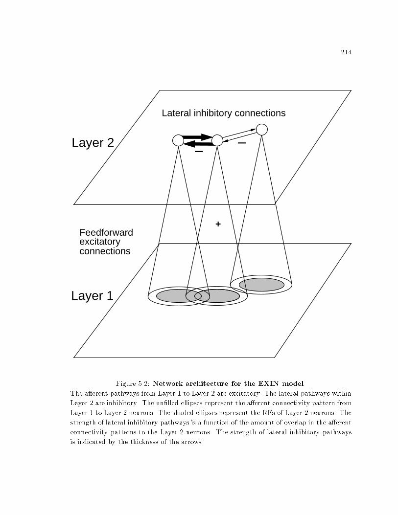
214Layer 2

Layer 1

Feedforward excitatoryconnections

+

Lateral inhibitory connections

Figure 5.2: Network architecture for the EXIN model.The a�erent pathways from Layer 1 to Layer 2 are excitatory. The lateral pathways withinLayer 2 are inhibitory. The un�lled ellipses represent the a�erent connectivity pattern fromLayer 1 to Layer 2 neurons. The shaded ellipses represent the RFs of Layer 2 neurons. Thestrength of lateral inhibitory pathways is a function of the amount of overlap in the a�erentconnectivity patterns to the Layer 2 neurons. The strength of lateral inhibitory pathwaysis indicated by the thickness of the arrows.

215If two neurons are only rarely coactivated then their reciprocal lateral inhibitory weightsbecome weak. Strong lateral inhibition between two neurons tends to make them less likelyto be coactivated, causing the two to become selective to di�erent inputs according tothe excitatory synaptic plasticity rule (Equation 5.2). Thus, when the network is exposedto normal stimuli, the lateral inhibitory weights and the excitatory a�erent weights aremodi�ed so that each neuron becomes selective to di�erent inputs and the RFs of all Layer 2neurons cover the input space (Marshall, 1995a; Marshall & Gupta, 1998). This leads toimproved discrimination and sparse coding (Marshall, 1995a).The EXIN a�erent excitatory synaptic plasticity ruleThe a�erent excitatory weight changes are governed by a variant of a Hebbianlearning rule. The rule can be expressed (Grossberg, 1982; Marshall, 1995a) asddtZ+ij;pq = � F(xpq) ��Z+ij;pq + H(xij)� ; (5.2)where � > 0 is a small learning rate constant, and F and H are half-recti�ed non-decreasingfunctions.Thus, whenever a neuron is active, its input excitatory connections from activeneurons tend to become slightly stronger, while its input excitatory connections from inactiveneurons tend to become slightly weaker. As discussed for Equation 5.1, the weight values inEquation 5.2 remain bounded.The EXIN excitatory synaptic plasticity rule is an instar competitive learning rule.When used in conjunction with strong lateral inhibition, it causes model cortical neuronsto become selective for a speci�c pattern of input activations (Marshall, 1995a).Stability of EXIN networksLike other competitive learning rules, the EXIN rules do not produce absolutelystable synaptic weights. The stability of the network depends on the input environment.If the input distribution changes for a su�ciently long time, the weights change to encodethe new statistics. Such instability, re ecting the statistics of the input environment is

216advantageous at lower-levels of cortical processing; e.g., the cortex can reorganize aftercortical or peripheral damage.The learning rates in competitive learning networks must be kept small enough toallow approximate stability in a statistically stationary input environment, yet large enoughto allow plasticity in response to the statistical changes posed by perturbations such asscotomas. Stability in competitive learning networks and the various learning parametersare discussed in Appendix C, Section C.1.2.Explanation of dynamic RF changes based on the EXIN rulesThe maximum extent of a Layer 2 neuron's RF is limited by the axonal arborizationspread of the Layer 1 neurons from which it receives a�erent excitation. In addition, aLayer 2 neuron receives lateral inhibition from neurons with which it is frequently co-excited.Neurons in Layer 2 can be consistently co-excited if they share inputs from common Layer 1neurons. Because of inhibition, it is possible that a Layer 2 neuron (p; q) does not becomeactive in response to some active Layer 1 neuron (i; j), even though Z+ij;pq > 0.The role of the EXIN a�erent excitatory and lateral inhibitory synaptic plasticityrules in producing RF changes during scotoma conditioning are studied independently.Role of EXIN lateral inhibitory synaptic plasticity. Consider the EXIN networkwith the a�erent excitatory synaptic plasticity rule disabled and the lateral inhibitorysynaptic plasticity rule enabled. When the network is exposed to scotoma stimuli witha su�ciently large scotoma, there exists a cortical scotoma region in Layer 2. Duringscotoma conditioning, neurons outside the cortical scotoma region are active and thoseinside the cortical scotoma region are not. Let neuron (p; q) be outside and neuron (r; s)be inside the initial cortical scotoma region (Figure 5.3a). Assume that after conditioningwith normal stimuli, Z�pq;rs and Z�rs;pq are not zero, because neurons (p; q) and (r; s) sharecommon a�erent inputs. If for a given stimulus, neuron (p; q) is active, then accordingto the EXIN inhibitory synaptic plasticity rule, Z�pq;rs weakens (Figure 5.3b). However,Z�rs;pq is unchanged, since xrs is zero. Thus, lateral inhibitory weights to neuron (r; s) fromactive neurons outside the cortical scotoma region weaken, but lateral inhibitory weightsfrom neuron (r; s) are una�ected. The net e�ect, from the point of view of neuron (r; s), is

217that its a�erent excitatory input weights remain unchanged and its input lateral inhibitoryweights from neurons outside the cortical scotoma region weaken (if nonzero before theconditioning). If the RF of neuron (r; s) is measured then, it will be more responsive topositions in its old RF and will be responsive to some new positions too (Figure 5.3b), thusproducing RF expansion. The simulation results are presented in Section 5.3.1.When the network is again conditioned with normal stimuli, the asymmetric lateralinhibitory weights between the neurons inside and outside the cortical scotoma region regainsymmetry. Thus, the RFs of neurons in the cortical scotoma are restored.Role of EXIN a�erent excitatory synaptic plasticity. Now consider the EXINnetwork with the lateral inhibitory synaptic plasticity rule disabled and the a�erentexcitatory synaptic plasticity rule enabled. Neurons close to the edge of the corticalscotoma but outside it show some interesting changes (e.g., neuron (p; q) in Figure 5.3c).Because these neurons are near the cortical scotoma edge, the region of their RF insidethe scotoma is not stimulated. Thus, because of the EXIN excitatory synaptic plasticityrule, a�erent excitatory connections from Layer 1 neurons in the scotoma region to thisneuron become weaker. Hence its RF shrinks, and the center of its RF shifts outward.During RF measurement after scotoma conditioning, these neurons (e.g., (p; q)) respondonly weakly to stimuli in the scotoma region and hence exert less inhibition on neuronsthat were inactive during conditioning (e.g., (r; s)). Thus, the neurons that were inactiveduring the conditioning show increased responsiveness and RF expansion. This explanationfor RF expansion during scotoma conditioning was proposed by Sirosh et al. (1996). TheRF expansion causes the RF centers to shift away from the scotoma center (Section 5.3.2).When the EXIN network with only a�erent excitatory synaptic plasticity enabledis conditioned again using normal stimuli, the neurons do not recover their original RFs.The neurons whose a�erent excitatory pathways from the scotoma region were weakenedare weakly actived by stimulation of the region that was occluded during arti�cial scotomaconditioning, during the subsequent whole-�eld stimulation. On the other hand, the neuronswhose initial RF was inside the scotoma region during arti�cial scotoma conditioning aremore responsive to positions inside the scotoma during whole-�eld stimulation, followingarti�cial scotoma conditioning. Thus, during whole-�eld stimulation following arti�cial

218Layer 2

Layer 1

pq

rs

(a)

pq

Ret

inal

sco

tom

a

regi

on

Cor

tical

sco

tom

a

regi

on

Layer 2

Layer 1

Cor

tical

sco

tom

a

regi

on

Ret

inal

sco

tom

a

regi

on

pq

rs

(b)

pq

Lateral inhibitory weight changes

Layer 2

Layer 1

pq

rs

(c)

pq

Ret

inal

sco

tom

a

regi

on

Cor

tical

sco

tom

a

regi

on

Afferent excitatory weight changes

Figure 5.3: Legend on next page.

219Figure 5.3: The e�ects of scotoma conditioning on the EXIN model.Figure on previous page. The un�lled ellipses represent the a�erent connectivity patternfrom Layer 1 to Layer 2 neurons. The shaded ellipses represent the RFs of Layer 2 neurons.The parallelogram within Layer 1 represents the scotoma region, and the parallelogramwithin Layer 2 represents the cortical scotoma region before scotoma conditioning. (a) Thenetwork state before scotoma conditioning. Neuron (r; s) is in the cortical scotoma regionbecause its RF is within the scotoma region; neuron (p; q) is outside the cortical scotomaregion. (b) The network state after scotoma conditioning with only lateral inhibitorysynaptic plasticity enabled. After scotoma conditioning, lateral inhibitory connectionsbetween neurons in the cortical scotoma and lateral inhibitory connections between neuronsoutside the cortical scotoma do not change. However, lateral inhibitory connections fromneurons outside the cortical scotoma (e.g., (p; q)) to neurons inside the cortical scotoma(e.g., (r; s)) weaken (dashed line). The decrease in inhibition received by neuron (r; s) resultsin expansion of its RF. (c) The network state after scotoma conditioning with only a�erentexcitatory synaptic plasticity enabled. After scotoma conditioning, a�erent connectionsto neurons in the cortical scotoma do not change. However, a�erent connections fromlocations inside the scotoma to neurons outside the cortical scotoma (e.g., (p; q)) weaken(dashed line). Neurons inside the cortical scotoma (e.g., (r; s)) receive less inhibition fromneuron (p; q) when locations inside the scotoma are stimulated. Thus, neuron (r; s) showsnew responsiveness to these locations, and its RF size thus increases.scotoma conditioning, the neurons whose initial RF was inside the scotoma region strengthena�erent excitatory pathways from positions inside the scotoma region to which they are moreresponsive and exert greater inhibition on neurons whose initial RF straddled the scotomaboundary. The neurons whose RF straddled the scotoma boundary further weaken a�erentexcitatory pathways from positions inside the scotoma region to which they have become lessresponsive after arti�cial scotoma conditioning, as their responsiveness to positions insidethe scotoma region is further suppressed. With strong �xed lateral inhibitory pathwaysweights, the lateral inhibition between neurons suppresses the activation of the neuronswhose RF size was decreased (because of weakening of pathways from the scotoma duringscotoma conditioning) when inputs are presented at positions inside the scotoma. Accordingto the EXIN a�erent excitatory synaptic plasticity rule, a�erent pathway weights changeonly when postsynaptic neurons are active. Thus, the weak a�erent connections from thescotoma region to the neurons whose RF size was decreased are not strengthened, and theRFs of these neurons do not shift back to their original positions (Section 5.3.2).

220In the EXIN network (with either lateral inhibitory or a�erent excitatory synapticplasticity alone), in response to scotoma stimuli, all neurons that show RF expansion belongto the set of neurons that were inside the initial cortical scotoma. Thus, after scotomaconditioning, the EXIN network with both lateral inhibitory and a�erent excitatory synapticplasticity will produce RF expansion in neurons that were inside the initial cortical scotoma.The activation equationThe activation level xpq of each Layer 2 neuron is governed by a shunting equation(Grossberg, 1972) based on the Hodgkin (Hodgkin, 1964) model:ddtxpq = �Axpq + �(B � xpq)Epq � (C + xpq)Ipq; (5.3)where A;B, C, �, and are constants, and Epq and Ipq represent respectively the neuron'stotal a�erent excitatory and lateral inhibitory input signals. Because Equation 5.3 is ashunting equation, if xpq(0) 2 [�C;B] then xpq(t) 2 [�C;B] for all time t � 0 (Cohen &Grossberg, 1983). Thus, activation levels are forced to remain within a bounded range,between �C and B. The total input excitation Epq is de�ned asEpq = 0@Xij [xij ]Z+ij;pq1A2 ; (5.4)and the total input inhibition Ipq is given byIpq =Xrs [xrs]Z�rs;pq; (5.5)where [a] � max(a; 0). Parameters � and , respectively, control the e�ectiveness of theexcitation and inhibition received by a Layer 2 neuron. The squaring in Equation 5.4sharpens the RF pro�le of the Layer 2 neurons; squaring enhances excitation to Layer 2neurons when Prs[xrs]Z�rs;pq > 1 and suppresses excitation to Layer 2 neurons whenPrs[xrs]Z�rs;pq < 1.Stability of the shunting equation: Cohen-Grossberg theoremThe shunting equation (Equation 5.3) with Z�rs;pq = Z�pq;rs � 0, belongs to a classof competitive dynamical systems that are absolutely stable; i.e., the system has �xed points

221for any choice of parameters (Cohen & Grossberg, 1983). The neuronal activations in sucha system are guaranteed to reach stable equilibrium values for all synaptic weight valueswith the restriction.However, it is not known whether the shunting equation remains absolutely stableeven when Z�rs;pq 6= Z�pq;rs � 0 for some pairs of neurons. The symmetry of reciprocalpairs of lateral inhibitory weights is not guaranteed by the EXIN lateral inhibitory synapticplasticity rule. During normal stimulation, the lateral inhibitory weights are approximatelysymmetric (Marshall, 1995a). They become asymmetric between neurons across thescotoma boundary during scotoma conditioning. Nevertheless, simulations empirically showthe stability of the EXIN network (Section C.1.1).The initial weightsIn the EXIN simulations, the initial a�erent excitatory weight from Layer 1neuron (i; j) to Layer 2 neuron (p; q) is given byZ+ij;pq(0) = "� exp �(x2 + y2)�2� ! ;��# ; (5.6)where [a; b] � 8><>: a if a > b;0 otherwise; (5.7)x; y 2 f�15; � � � ; 14g, p = (((i+15)+x) mod 30)�15, and q = (((j+15)+y) mod 30)�15.The indices i; j; p; and q are in f�15; � � � ; 14g. The indices i; j; p; and q and thedistances x and y are related by the above equations because the model cortical and thalamicneurons are arranged in a wrapped-around two-dimensional grid. The parameters , �� ,and �� are positive constants.The initial lateral inhibitory weights between Layer 2 neurons (p; q) and (r; s),where p 6= r or q 6= s, are set as follows. LetXpq;rs =Xij min(Z+ij;pq; Z+ij;rs) (5.8)and W�pq;rs(0) = W�rs;pq(0) = [Xpq;rs;�i] ; (5.9)

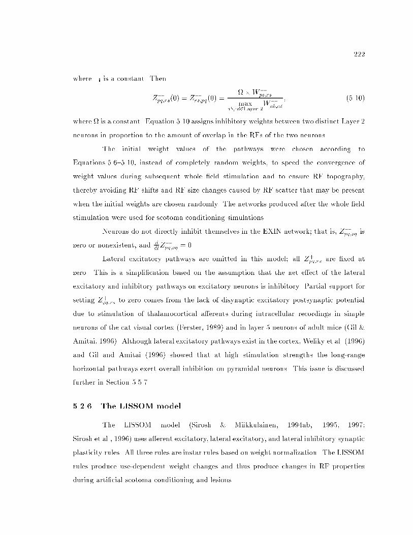
222where �i is a constant. ThenZ�pq;rs(0) = Z�rs;pq(0) = �W�ps;rsmaxab;cd2Layer 2W�ab;cd ; (5.10)where is a constant. Equation 5.10 assigns inhibitory weights between two distinct Layer 2neurons in proportion to the amount of overlap in the RFs of the two neurons.The initial weight values of the pathways were chosen according toEquations 5.6{5.10, instead of completely random weights, to speed the convergence ofweight values during subsequent whole �eld stimulation and to ensure RF topography,thereby avoiding RF shifts and RF size changes caused by RF scatter that may be presentwhen the initial weights are chosen randomly. The networks produced after the whole �eldstimulation were used for scotoma conditioning simulations.Neurons do not directly inhibit themselves in the EXIN network; that is, Z�pq;pq iszero or nonexistent, and ddtZ�pq;pq = 0.Lateral excitatory pathways are omitted in this model; all Z+pq;rs are �xed atzero. This is a simpli�cation based on the assumption that the net e�ect of the lateralexcitatory and inhibitory pathways on excitatory neurons is inhibitory. Partial support forsetting Z+pq;rs to zero comes from the lack of disynaptic excitatory postsynaptic potentialdue to stimulation of thalamocortical a�erents during intracellular recordings in simpleneurons of the cat visual cortex (Ferster, 1989) and in layer 5 neurons of adult mice (Gil &Amitai, 1996). Although lateral excitatory pathways exist in the cortex, Weliky et al. (1996)and Gil and Amitai (1996) showed that at high stimulation strengths the long-rangehorizontal pathways exert overall inhibition on pyramidal neurons. This issue is discussedfurther in Section 5.5.7.5.2.6 The LISSOM modelThe LISSOM model (Sirosh & Miikkulainen, 1994ab, 1995, 1997;Sirosh et al., 1996) uses a�erent excitatory, lateral excitatory, and lateral inhibitory synapticplasticity rules. All three rules are instar rules based on weight normalization. The LISSOMrules produce use-dependent weight changes and thus produce changes in RF propertiesduring arti�cial scotoma conditioning and lesions.

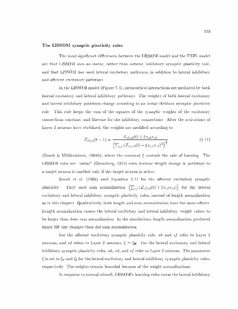
223The LISSOM synaptic plasticity rulesThe most signi�cant di�erences between the LISSOM model and the EXIN modelare that LISSOM uses an instar, rather than outstar, inhibitory synaptic plasticity rule,and that LISSOM has used lateral excitatory pathways, in addition to lateral inhibitoryand a�erent excitatory pathways.In the LISSOM model (Figure 5.4), intracortical interactions are mediated by bothlateral excitatory and lateral inhibitory pathways. The weights of both lateral excitatoryand lateral inhibitory pathways change according to an instar Hebbian synaptic plasticityrule. This rule keeps the sum of the squares of the synaptic weights of the excitatoryconnections constant, and likewise for the inhibitory connections. After the activations ofLayer 2 neurons have stabilized, the weights are modi�ed according toZab;cd(t+ 1) = Zab;cd(t) + �xabxcd�Pef (Zef;cd(t) + �xefxcd)2� 12 (5.11)(Sirosh & Miikkulainen, 1994b), where the constant � controls the rate of learning. TheLISSOM rules are \instar" (Grossberg, 1972) rules because weight change in pathways toa target neuron is enabled only if the target neuron is active.Sirosh et al. (1996) used Equation 5.11 for the a�erent excitatory synapticplasticity. They used sum normalization �Pef (Zef;cd(t) + �xefxcd)� for the lateralexcitatory and lateral inhibitory synaptic plasticity rules, instead of length normalizationas in this chapter. Qualitatively, both length and sum normalization have the same e�ects.Length normalization causes the lateral excitatory and lateral inhibitory weight values tobe larger than does sum normalization. In the simulations, length normalization producedlarger RF size changes than did sum normalization.For the a�erent excitatory synaptic plasticity rule, ab and ef refer to Layer 1neurons, and cd refers to Layer 2 neurons, � = �� . For the lateral excitatory and lateralinhibitory synaptic plasticity rules, ab, cd , and ef refer to Layer 2 neurons. The parameter� is set to �e and �i for the lateral excitatory and lateral inhibitory synaptic plasticity rules,respectively. The weights remain bounded because of the weight normalizations.In response to normal stimuli, LISSOM's learning rules cause the lateral inhibitory

224Layer 2

Layer 1

Afferent excitatoryconnections

+

++

++ +

+

+

+

Lateral excitatory and inhibitory connections

rs pquv

+

+

Figure 5.4: Network architecture for the LISSOM model and theinhibition-dominant adaptation model.The connections from Layer 1 to Layer 2 are excitatory. There are lateral inhibitory andexcitatory connections between Layer 2 neuron (p; q) and Layer 2 neurons within the innerellipse (e.g., (r; s)). Neuron (p; q) also sends both inhibitory and excitatory connectionsto itself. The lateral connections between neuron (p; q) and Layer 2 neurons (e.g., (u; v))outside the inner ellipse and inside the outer ellipse are inhibitory. The un�lled ellipses inLayer 1 represent the a�erent connectivity pattern from Layer 1 to Layer 2 neurons. Theshaded ellipses represent the RFs of Layer 2 neurons.

225and lateral excitatory weights between pairs of Layer 2 neurons to remain approximatelysymmetric. In addition, the lateral inhibitory and excitatory weights become approximatelyproportional to the amount of coactivation between neuron pairs. The learning rulesmaintain the initial topographically arranged RFs (Sirosh & Miikkulainen, 1997).Stability of LISSOM networksThe LISSOM learning rules are competitive learning rules. Therefore, the stabilityof LISSOM networks depends on the input environment and the learning rates (Sirosh &Miikkulainen, 1994b). This issues of network stability and choice of the various parametersin the current simulations are discussed in Appendix C, Section C.2.Explanation of dynamic RF changes based on LISSOM rulesThe e�ect of each of the three LISSOM synaptic plasticity rules is consideredseparately. The overall behavior of the LISSOM model depends on the relative learningrates of the three rules.Role of LISSOM lateral inhibitory synaptic plasticity. Consider the LISSOMnetwork with only the lateral inhibitory synaptic plasticity rule enabled. Let neuron (p; q)be outside and neuron (r; s) be inside the cortical scotoma region. Assume that afterconditioning with normal stimuli, Z�pq;rs and Z�rs;pq are not zero, because neurons (p; q) and(r; s) share some common a�erent inputs, and that they are approximately equal. Accordingto the LISSOM lateral inhibitory synaptic plasticity rule, Z�pq;rs does not change, becausexrs is 0. However, Z�rs;pq decreases if some other neuron (u; v) is active, because the weightsare normalized. In addition, the normalization causes the lateral inhibitory weights fromactive neurons (e.g, neurons (u; v) and (p; q)) to neuron (p; q) to become slightly stronger.In the LISSOM model, Layer 2 neurons send lateral excitatory and inhibitory pathways tothemselves. Thus, because of the lateral inhibitory synaptic plasticity, neurons outside thecortical scotoma region receive a reduced overall amount of inhibition from neurons withinthe cortical scotoma. This causes neurons like (p; q) that are outside the cortical scotomaregion to exhibit increased responsiveness, a RF expansion, and a slight inward RF shifttoward the scotoma edge. The RF expansion of neuron (p; q) is asymmetric because it

226receives reduced inhibition only when the input is in the scotoma region. For neurons in theoverall excitatory zone of neuron (p; q) (e.g., (u; v) and (r; s)), the increased responsivenessof neuron (p; q) may result in increased responsiveness, a RF expansion, and a slight inwardRF shift toward the scotoma edge. The increased responsiveness of (p; q) results in increasedinhibition to neurons in the overall inhibitory zone of neuron (p; q) (e.g., (c; d) and (a; b))(Figure 5.5b), when input locations inside the scotoma are stimulated. Because of theasymmetric RF pro�le, neurons whose initial RF center is inside the scotoma and in theoverall inhibitory zone of neuron (p; q) (e.g., (a; b)) would show decreased responsiveness,RF contraction, and a small inward RF shift away from the scotoma edge (Figure 5.5b).The simulation results are in Section 5.3.1.Role of LISSOM lateral excitatory synaptic plasticity. When only the LISSOMlateral excitatory synaptic plasticity rule is enabled, Z+pq;rs does not change, Z+rs;pq decreases,and the lateral excitatory weights from active neurons (e.g, neurons (u; v) and (p; q)) toneuron (p; q) become slightly stronger (in the LISSOM network neurons receive lateralexcitatory pathways from itself), for the same reasons described in the previous paragraph(Figure 5.5c). Thus, neurons outside the cortical scotoma region receive a reducedamount of lateral excitation from neurons in the cortical scotoma. This results in reducedresponsiveness, decreased RF size, and an outward RF shift, away from the scotoma edge,for neurons like (p; q) that are outside the cortical scotoma region. For neurons in theoverall excitatory zone of neuron (p; q) (e.g., (u; v) and (r; s)), the decreased responsivenessof neuron (p; q) may result in decreased responsiveness, a RF contraction, and a slightoutward RF shift away from the scotoma edge. For neurons in the overall inhibitory zone ofneuron (p; q) (e.g., (c; d) and (a; b)), the decreased responsiveness of (p; q) results in reducedinhibition. Active neurons during scotoma conditioning receive weakened lateral excitatorysignals from neurons inside the cortical scotoma. These asymmetric lateral excitatoryweight changes lead to a decrease in RF size and an outward RF shift away from thescotoma in neurons whose initial RF center is close to the scotoma boundary (e.g., (p; q)).They also lead to an increase in RF size and an outward RF shift away from the scotomacenter in neurons (e.g., (a; b)) whose initial RF is inside and close to the scotoma boundary(Figure 5.5c). The simulation results are shown in Section 5.3.3.

227R

etin

al s

coto

ma

regi

on

Layer 2

Layer 1

cd uv rs ab

(a)

pq

Cor

tical

sco

tom

a re

gion

Layer 2

Layer 1

(b)

Ret

inal

sco

tom

a re

gion

Cor

tical

sco

tom

a re

gion

Lateral inhibitory weight changes

cd uv rs abpq

Layer 2

Layer 1

(c)

Cor

tical

sco

tom

a re

gion

Ret

inal

sco

tom

a re

gion

Lateral excitatory weight changes

cd uv rs abpq

Layer 2

Layer 1

cd rs ab

(d)

pquv

Cor

tical

sco

tom

a re

gion

Ret

inal

sco

tom

a re

gion

Afferent excitatory weight changes

Figure 5.5: Legend on next page.

228Figure 5.5: The e�ects of scotoma conditioning on the LISSOM model.Figure on previous page. The un�lled ellipses in Layer 1 represent the a�erent connectivitypattern from Layer 1 to Layer 2 neurons. The shaded ellipses represent the RFs ofLayer 2 neurons. The parallelogram within Layer 1 represents the scotoma region, andthe parallelogram within Layer 2 represents the cortical scotoma region before scotomaconditioning. (a) The network state before scotoma conditioning. Neurons (r; s) and(a; b) are inside the cortical scotoma region because their RFs are within the scotomaregion. Neurons (p; q), (u; v), and (c; d) are outside the cortical scotoma region. Thereare excitatory and inhibitory connections between neuron (p; q) and neurons in the smallellipse (e.g., (u; v) and (r; s)). The connections between neuron (p; q) and the neuronsoutside the small ellipse and inside the large ellipse are inhibitory. (b) The network stateafter scotoma conditioning with only instar lateral inhibitory synaptic plasticity enabled.The dashed lines represent a decrease in the connection weights and the thick lines representan increase in the connection weights. (c) The network state after scotoma conditioningwith only instar lateral excitatory synaptic plasticity enabled. (d) The network state afterscotoma conditioning with only a�erent excitatory synaptic plasticity enabled.Role of LISSOM a�erent excitatory synaptic plasticity. In the LISSOM networkwith only a�erent excitatory synaptic plasticity enabled, the synaptic plasticity causeschanges in the a�erent connectivity of neurons close to the edge of the cortical scotomaregion (Figure 5.5d). These neurons (e.g., (u; v) and (p; q)) have part of their input inLayer 1 within the scotoma. Thus, according to the a�erent excitatory synaptic plasticityrule, when these neurons are activated, the weights from neurons within the scotoma becomeweaker, and weights from Layer 1 neurons outside the scotoma become stronger. This causesthe RFs of Layer 2 neurons (e.g., (u; v) and (p; q)) close to the initial cortical scotomaedge to shrink and shift away from the scotoma center. In addition, these neurons respondweakly to stimulation at positions in the scotoma region and exert less inhibition on neurons(e.g., (a; b)) that were inactive during conditioning. Thus, the neurons that were inactiveduring the conditioning show increased responsiveness and RF expansion away from thescotoma center (Sirosh et al., 1996). The RF expansion causes the RF centers to shift awayfrom the scotoma center (Figure 5.5d). The simulation results are in Section 5.3.2.The overall e�ect on responsiveness, RF size, and RF position depends on therelative strengths and sizes of a�erent excitation, lateral excitation, and lateral inhibition.It also depends on the learning rates of the three types of connections. In the LISSOM

229model, the e�ects of inhibitory synaptic plasticity are in con ict with the e�ects of a�erentand lateral excitatory synaptic plasticity. The RF expansion occurs in neurons outside thecortical scotoma if the relative strength and learning rate of lateral inhibitory weights aregreater than those of the lateral and a�erent excitatory weights. The RF expansion occursin neurons inside the cortical scotoma if the relative strength and learning rate of lateralexcitatory or a�erent excitatory weights are greater than those of the lateral inhibitoryweights. After arti�cial scotoma conditioning, the LISSOM rules produce RF expansion onone side of the scotoma boundary and RF contraction on the other side.When the LISSOM networks (with plasticity in only one of the three types ofpathways) are again conditioned with normal stimuli, the RFs of all a�ected neurons arerestored.The activation equationIn the LISSOM simulations, the Layer 2 neuron activations are determinediteratively byxpq(t+ 1) = S0@ � Xij Z+ij;pqxij(t) + eXrs Z+rs;pqxrs(t)� iXrs Z�rs;pqxrs(t)1A (5.12)where S(a) = 11 + exp (� [a]) � 0:5 (5.13)(Sirosh & Miikkulainen, 1994b), and [x] = max(0; x). The constants � , e and i arescaling factors on the excitatory and inhibitory weights and determine the strength ofa�erent and lateral interactions. The activations are bounded because of the sigmoidfunction S.Stability of LISSOM activation equationThe LISSOM activation equation can quickly equilibrate (Sirosh &Miikkulainen, 1994b). Equation 5.12 approached a �xed point during the various inputconditioning regimes for the parameters that are used in this chapter (Appendix C,Section C.2.1).

230The initial weightsIn simulations using the LISSOM model, the connection weights were computedas follows. Let Yab;cd = "exp �(m2 + n2)�2 ! ;�# ; (5.14)where a; b; c; d;m;n 2 f�15; : : : ; 14g, c = (((a + 15) + m) mod 30) � 15, and d =(((b + 15) + n) mod 30) � 15. The relationship between the indices a; b; c; and d and thedistances m and n is such that the model cortical and thalamic neurons are arranged in awrapped-around two-dimensional grid. The paramters � and � are positive constants, andthe notation [:; :] is de�ned by Equation 5.7. ThenZab;cd(0) = Yab;cd�Pef Y 2ef;cd� 12 (5.15)is the initial weight of the connection pathway from neuron (a; b) to neuron (c; d).For a�erent weights, ab and ef refer to Layer 1 neurons, cd refers to Layer 2neurons, � = �� , and � = �� . For lateral excitatory and lateral inhibitory weights, ab, cd ,and ef refer to Layer 2 neurons. For lateral excitatory weights, � = �e and � = �e, and forinhibitory weights, � = �i and � = �i.The initial weights were chosen to speed the simulations; in all simulations,these weight values were overridden by new values during an initial phase of whole-�eldstimulation.5.2.7 The inhibition-dominant adaptation modelXing and Gerstein (1994) described four models of dynamic RFs and argued infavor of an inhibition-dominant network with neural adaptation, or habituation. A neuron'sability to �re decreases/increases after a period of activity/inactivity, without any synapticchanges. In an inhibition-dominant adaptation network, the strength of the lateralinhibitory connections is greater than that of lateral excitatory connections, and all theweights are �xed.Xing and Gerstein used a spiking neuron model. They modeled adaptation bymodifying the action potential threshold, which depended on the number of spikes of a

231neuron in the recent past. Thus, if a neuron spikes frequently, its action potential thresholdincreases, thereby making it spike less vigorously, even though the same input is present.On the other hand, if a neuron has not been activated for a long time, then it becomeshighly responsive to inputs in its RF.The adaptation equationIn the present simulations the spiking neuron model is not used. Instead, theoutput of a Layer 2 neuron (p; q) is modeled as [xpq � Tpq ], where xpq is controlled by ashunting equation (Grossberg, 1972):ddtxpq = �Axpq + (B � xpq)Epq � (C + xpq)Ipq; (5.16)with Epq = �� Xi;j2Layer 1[xij ]Z+ij;pq + �e Xr;s2Layer 2[xrs � Trs]Z+rs;pq; (5.17)Ipq = X(r;s)2Layer 2[xrs � Trs]Z�rs;pq; (5.18)and [a] � max(a; 0). The positive constants �� and �e control the e�ectiveness of a�erentexcitation and lateral excitation, respectively. The variable Tpq represents the adaptive �ringthreshold of neuron (p; q). After the activation of Layer 2 neurons has reached equilibrium,the adaptation parameter Tpq is modi�ed according toddtTpq = � (��Tpq + (� � Tpq) [xpq � Tpq ]) ; (5.19)where �, �, � are positive constants. The constant � controls the rate of change in Tpq. Theconstants � and � determine the maximum value of Tpq , and the relative rates of increaseand decrease in Tpq, respectively. As � increases the maximum value of Tpq decreases andthe rate of decrease in Tpq when [xrs � Trs] = 0 increases, and as � increases the maximumvalue of Tpq increases and the rate of increase in Tpq increases. According to Equation 5.19,if Tpq(0) � 0, then Tpq(t) � 0 for all t � 0. The threshold Tpq increases if neuron (p; q) wasactive in its recent past and decreases if (p; q) was not very active.The spiking model was not implemented here because Xing and Gerstein (1994)did not provide complete implementation details of their model. Even though the model

232described by Equations 5.16{5.19 di�ers from the spiking model used by Xing and Gersteinin their simulations, it captures the essential characteristics of their inhibition-dominantadaptation model: the simulation results based on Equations 5.16{5.19 replicate theirresults. In the inhibition-dominant adaptation network, the lateral inhibitory and lateralexcitatory pathway weights are symmetric. Extensive simulations show that the systemde�ned by Equation 5.16 may be absolutely stable (Cohen & Grossberg, 1983). Simulationspresented in this chapter show that the network equilibrates. The adaptation levels of theneurons reach stable �xed points with su�cient training. The initial pathway weights areset according to Equations 5.14 and 5.15.Explanation of dynamic RF changes based on adaptationAfter the network receives normal stimulation for a su�ciently long time, everyLayer 2 neuron becomes adapted by approximately the same amount. In response to thescotoma stimuli, the neurons outside the cortical scotoma region are activated, therebykeeping them habituated. However, the inactive neurons whose RF is inside the scotomabecome dishabituated. Dishabituation of neurons with RF inside the scotoma producesincreased responsiveness and RF expansion. The increased responsiveness increasesinhibition to neurons whose RF is outside the scotoma. Thus, the RF size of the neuronswhose RF is occluded by the scotoma region increases, and the RF size of some neuronswhose RF is just outside the scotoma decreases. As scotoma conditioning proceeds, someneurons in the initial cortical scotoma may recover functionality. As in the EXIN model, allneurons that show RF expansion are those whose RF lies within the scotoma (Figure 5.6).If the network is exposed to normal stimuli again, the RF of the neurons that werein the cortical scotoma region is restored. The simulation results are in Section 5.3.1.The above explanation is di�erent from the one given by Xing and Gerstein (1994).In their simulations, they measured the initial RFs before any conditioning by the normalstimuli. Then they conditioned the network using scotoma stimuli. In this case, the neuronsin the cortical scotoma region are not a�ected, and those outside the cortical scotomaadapt. The adaptation of the neurons outside the cortical scotoma causes them to be less

233R

etin

al s

coto

ma

regi

on

Layer 2

Layer 1

(a)

Cor

tical

sco

tom

a re

gion

Ret

inal

sco

tom

a re

gion

Layer 2

Layer 1

(b)

Cor

tical

sco

tom

a re

gion

Figure 5.6: The e�ects of scotoma conditioning on the inhibition-dominantadaptation model.The un�lled ellipses represent the a�erent connectivity pattern from Layer 1 to Layer 2neurons. The shaded ellipses represent the RFs of Layer 2 neurons. The parallelogramwithin Layer 1 represents the scotoma region, and the parallelogram within Layer 2represents the cortical scotoma region before scotoma conditioning. (a) The network statebefore scotoma conditioning. All Layer 2 neurons have almost the same adaptation level(shaded circles). Thus, all Layer 2 neurons have almost the same RF size. (b) The networkstate after scotoma conditioning. The neurons inside the cortical scotoma are dishabituated(white circles) and hence are highly responsive to input stimulation. The neurons insidethe cortical scotoma inhibit neurons outside the cortical scotoma and in turn receive weakerinhibition. Thus, neurons within the cortical scotoma show RF expansion.responsive, and hence they exert less inhibition on neurons in the cortical scotoma. As aresult, the size of the RF of the neurons in the scotoma region increases (see Section 5.3.1).The conditioning procedure used by Xing and Gerstein di�ers from that used by Pettet andGilbert (1992). In the experiments of Pettet and Gilbert, the original RF was determinedafter a period of random stimulation within and outside the �eld.In the inhibition-dominant adaptation model used in simulations presented in thischapter, if the Tpq values had not equilibrated during normal stimuli presentations, thenthey would increase for neurons outside the cortical scotoma and would decrease for thosein the cortical scotoma. This situation would also produce expansion of the RF of neurons

234in the cortical scotoma.5.2.8 The adaptation model with no lateral interactionIn this variant of the adaptation model, there are no lateral excitatory or lateralinhibitory pathways. The neurons adapt according to Equation 5.19. In the simulations,the activation level of Layer 2 neuron (p; q) is [xpq � Tpq ], where xpq is controlled byEquation 5.16. With no lateral interactions, Equation 5.16 can be solved analytically(Appendix C, Section C.3.1). The a�erent excitatory weights were the same as for theinhibition-dominant network.Explanation of dynamic RF changes based on adaptationIn the adaptation network with no lateral interactions, all the neurons are adaptedequally after normal stimulation. During scotoma conditioning, neurons with initial RFs inthe scotoma region dishabituate due to inactivity. As the adaptation level in neurons withinthe cortical scotoma decreases, the e�ective RF size of these neurons increases. Neuronsoutside the cortical scotoma remain adapted because of activation by the input stimuli.During normal stimulation following scotoma conditioning, the previously inactive neuronsare activated; hence they become adapted, and their RF size contracts. In the absenceof lateral interactions, the RFs remain symmetric, and there are no shifts in RF positionduring scotoma conditioning. Simulation results are in Section 5.3.1.5.2.9 The excitation-dominant adaptation modelIn an excitation-dominant adaptation network, the strength of the lateralexcitatory connections is greater than that of lateral inhibitory connections. In this model,the neurons adapt according to Equation 5.19. The output of Layer 2 neuron (p; q) is[xpq � Tpq ], where xpq is controlled by Equation 5.16. The initial connection weights areset according to Equation 5.15. In the simulations, the activation equation equilibrated(Appendix C, Section C.3.1).

235Explanation of dynamic RF changes based on adaptationIn the excitation-dominant adaptation network, all the neurons are adapted equallyafter normal stimulation. During scotoma conditioning, neurons with initial RF in thescotoma region become less adapted, because of inactivity. The neurons close to the center ofthe cortical scotoma become least adapted and hence most responsive. In addition, becauseof lateral excitation, the neighboring neurons excite one another. Thus, neurons within thecortical scotoma show RF expansion. Since neurons receive more lateral excitation fromneurons within the cortical scotoma, the RFs of the neurons shift toward the center of thescotoma. Neurons outside the cortical scotoma remain adapted because of activation by theinput stimuli. During normal stimulation following scotoma conditioning, the previouslyinactive neurons are activated; hence they become adapted, and their RF size contracts.Simulation results are in Section 5.3.1.5.3 Simulation results: Scotoma stimuliThe simulation results are organized to emphasize the e�ects of the di�erent rulesfor RF changes after arti�cial scotoma conditioning and retinal lesions. The di�erentsynaptic plasticity rules in the EXIN and the LISSOM model serve di�erent purposes duringself-organization of various cortical properties. The analyses of the e�ects of each ruleindividually during arti�cial scotoma conditioning and retinal lesions elucidates the uniqueproperties of the rules. Furthermore, the dynamic RF changes produced by the full EXINand the full LISSOM model during arti�cial scotoma conditioning depend on the relativelearning rates of the di�erent synaptic plasticity rules, and thus the e�ects produced by onerule can mask the e�ects produced by the others.In Section 5.3.1, the EXIN network with only lateral inhibitory synaptic plasticityenabled, the LISSOM network with only lateral inhibitory synaptic plasticity enabled, theinhibition-dominant adaptation network, the adaptation network with no lateral interaction,the excitation-dominant adaptation network, and the inhibition-dominant adaptationnetwork with no prior normal stimulation are simulated during scotoma conditioning. Theseresults are compared to experimental data. In Section 5.3.2, the e�ects of synaptic plasticity

236in a�erent excitatory pathways alone in the EXIN and LISSOM networks during scotomaconditioning are presented, and the e�ects of lateral excitatory synaptic plasticity aloneduring scotoma conditioning are presented in Section 5.3.3 using the LISSOM network. Tofurther distinguish the e�ects of the various rules for cortical plasticity, a novel experimentis presented in Section 5.4.5.3.1 Comparison of outstar/instar lateral inhibitory synaptic plasticityrules and neuronal adaptationThe following simulations highlight the opposite e�ects of instar and outstar lateralinhibitory synaptic plasticity rules.Dynamic RF expansion and contractionTo induce robust expansion and contraction of RF size, Pettet and Gilbert (1992)presented the arti�cial scotoma conditioning stimuli for several minutes. Becausequantitative mapping took several minutes, the exact time course of the observed changeswas not determined. To minimize the e�ect of the RF measurement process on the RF size,Pettet and Gilbert (1992) alternated conditioning stimuli and RF mapping. Pettet andGilbert (1992) reported that the RF expansion after arti�cial scotoma conditioning wasalways accompanied by an increased responsiveness from the region of the original RF.However, the spontaneous �ring of the neuron in the absence of visual stimuli did notchange. In the simulations, the synaptic plasticity rules and the adaptation rules wereturned-o� so that the RF sizes are not a�ected by RF measurements. Figure 5.7 comparesthe RF sizes of Layer 2 neurons that show maximal RF expansion after scotomaconditioning. Neurons with maximal RF expansion are shown to emphasize the asymmetryin the RF pro�le after arti�cial scotoma conditioning in the models. The RF expands inthe EXIN network with only lateral inhibitory synaptic plasticity enabled (Figure 5.7d) andin the inhibition-dominant adaptation network (Figure 5.7f) after scotoma conditioning, inneurons whose initial RF is inside the scotoma. In the LISSOM network with only lateralinhibitory synaptic plasticity enabled, the initial RF of the neuron that showed maximal

237RF expansion after scotoma conditioning was located outside the scotoma (Figure 5.7e).Re-conditioning with normal stimuli resulted in RF restoration in all the three models, asshown in Figures 5.7g{i. The simulations illustrate the qualitative behavior of the models.The absolute RF size and the absolute RF size change in the three networks are parameterdependent, and can be matched better with some parameter adjustments. Therefore, thedi�erences in the RF size and the absolute RF size change of model neurons in the modelsare not signi�cant.Pettet and Gilbert (1992) claimed that the expansion elicited by the arti�cialscotoma never exceeded the boundaries of the scotoma. However, the neurons thatthey studied had initial RFs in the center of the arti�cial scotoma, and the size ofthe scotoma was about three times the diameter of the initial RF. Darian-Smith andGilbert (1995) showed rapid recovery of responsiveness in neurons whose RF was insidethe cortical scotoma, following bilateral retinal lesions. This indicates that the RF of someneurons in the original cortical scotoma crossed the retinal scotoma boundary. The EXINnetwork with lateral inhibitory synaptic plasticity alone, the LISSOM network with onlylateral inhibitory synaptic plasticity enabled, and the inhibition-dominant adaptation modelproduced RF expansions that cross the scotoma boundaries (Figure 5.7).The RF expansions in the three simulations are accompanied by increasedresponsiveness of the corresponding Layer 2 neurons. Figures 5.8a{c compare theresponsiveness of the neurons whose RFs are shown in Figure 5.7, before and afterconditioning with scotoma stimuli in the three models. Note that after scotomaconditioning, the RF pro�le of some neurons in these models is asymmetric. Theasymmetric RF shape is caused by asymmetric changes of the weights in the EXINand LISSOM simulations and by asymmetric changes in adaptation level of the neuronsin the inhibition-dominant adaptation network. The asymmetry in the RF pro�leproduced by the EXIN and the inhibition-dominant adaptation networks is consistentwith observations made by Das and Gilbert (1995b), that neurons were more responsive tolocations outside the scotoma than to those inside, following arti�cial scotoma conditioning.DeAngelis et al. (1995) did not observe asymmetry in the RF of recorded neurons whoseRF was inside the scotoma during scotoma conditioning; this may have happened because

238

(g) (h) (i)

(d) (e) (f)

(a) (b) (c)

EXIN-LI

Initial

LISSOM-LI AN-ID

Scotoma

Reset

Figure 5.7: Legend on next page.

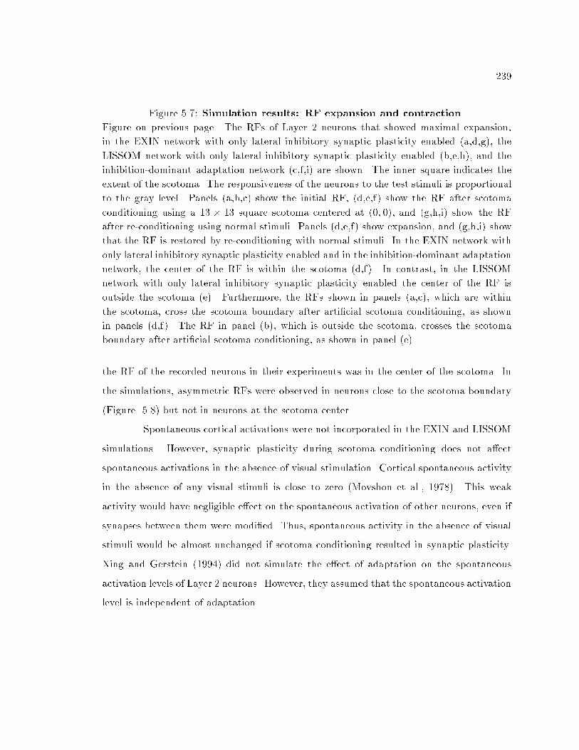
239Figure 5.7: Simulation results: RF expansion and contraction.Figure on previous page. The RFs of Layer 2 neurons that showed maximal expansion,in the EXIN network with only lateral inhibitory synaptic plasticity enabled (a,d,g), theLISSOM network with only lateral inhibitory synaptic plasticity enabled (b,e,h), and theinhibition-dominant adaptation network (c,f,i) are shown. The inner square indicates theextent of the scotoma. The responsiveness of the neurons to the test stimuli is proportionalto the gray level. Panels (a,b,c) show the initial RF, (d,e,f) show the RF after scotomaconditioning using a 13 � 13 square scotoma centered at (0; 0), and (g,h,i) show the RFafter re-conditioning using normal stimuli. Panels (d,e,f) show expansion, and (g,h,i) showthat the RF is restored by re-conditioning with normal stimuli. In the EXIN network withonly lateral inhibitory synaptic plasticity enabled and in the inhibition-dominant adaptationnetwork, the center of the RF is within the scotoma (d,f). In contrast, in the LISSOMnetwork with only lateral inhibitory synaptic plasticity enabled the center of the RF isoutside the scotoma (e). Furthermore, the RFs shown in panels (a,c), which are withinthe scotoma, cross the scotoma boundary after arti�cial scotoma conditioning, as shownin panels (d,f). The RF in panel (b), which is outside the scotoma, crosses the scotomaboundary after arti�cial scotoma conditioning, as shown in panel (e).the RF of the recorded neurons in their experiments was in the center of the scotoma. Inthe simulations, asymmetric RFs were observed in neurons close to the scotoma boundary(Figure 5.8) but not in neurons at the scotoma center.Spontaneous cortical activations were not incorporated in the EXIN and LISSOMsimulations. However, synaptic plasticity during scotoma conditioning does not a�ectspontaneous activations in the absence of visual stimulation. Cortical spontaneous activityin the absence of any visual stimuli is close to zero (Movshon et al., 1978). This weakactivity would have negligible e�ect on the spontaneous activation of other neurons, even ifsynapses between them were modi�ed. Thus, spontaneous activity in the absence of visualstimuli would be almost unchanged if scotoma conditioning resulted in synaptic plasticity.Xing and Gerstein (1994) did not simulate the e�ect of adaptation on the spontaneousactivation levels of Layer 2 neurons. However, they assumed that the spontaneous activationlevel is independent of adaptation.

240-14 -12 -10 -8 -6 -4 -2 0 2 4 6 8 10 12 14

012345678910

Neu

ron

activ

ityE

XIN

-LI

initialduring scotomareset

(a)

-14 -12 -10 -8 -6 -4 -2 0 2 4 6 8 10 12 14012345678910

Neu

ron

activ

ityLI

SS

OM

-LI

initialduring scotomareset

(b)

-14 -12 -10 -8 -6 -4 -2 0 2 4 6 8 10 12 14012345678910

Neu

ron

activ

ityA

N-I

D

Distance from scotoma center

initialduring scotomareset

(c)Figure 5.8: Simulation results: The iceberg e�ect.Layer 2 neuron responsiveness before scotoma conditioning (solid line), after scotomaconditioning (dashed line), and after re-conditioning with normal stimuli (dotted line)are shown. Neuron activations in the EXIN network with only lateral inhibitory synapticplasticity enabled (a), the LISSOM network with only lateral inhibitory synaptic plasticityenabled (b), and the inhibition-dominant adaptation network (c), are shown as a functionof one-dimensional input positions across Layer 1 passing through the scotoma center. Theresponsiveness is for the neurons in Figure 5.7. The responsiveness is computed by summingthe response of the Layer 2 neuron to test stimuli along the y axis at each x axis position.The neuron position is represented relative to the x coordinate of the scotoma center. Thescotoma is a square of size 13� 13. The thick line segment on the abscissa represents thescotoma region.

241RF size as a function of positionPettet and Gilbert (1992) showed RF expansion of cortical neurons whoseinitial RF was within the arti�cial scotoma, after conditioning with arti�cial scotomastimuli. Darian-Smith and Gilbert (1995) reported that between �ve minutes and one hourafter bilateral retinal lesions, cortical neurons located close to or just inside the corticalscotoma boundary showed a striking increase in RF size.Figures 5.9a{c show the RF size before and after scotoma stimuli conditioningas a function of the position of the initial RF center, for the three models. For theEXIN network with only lateral inhibitory synaptic plasticity enabled, Figure 5.9a, andthe inhibition-dominant adaptation model, Figure 5.9c, the most prominent RF expansionsoccur for Layer 2 neurons with initial RF centers close to and inside the scotoma edge.However, for the LISSOM network with only lateral inhibitory synaptic plasticity enabled,Figure 5.9b, the most prominent RF expansions occur for Layer 2 neurons with initialRF centers close to and outside the scotoma edge.RF size pro�le as a function of scotoma sizeIn the three simulations, neurons whose initial RF was close to the scotomaboundary showed the maximal expansion. This is clearly visible in the bimodal peaksin Figure 5.9. In the EXIN network with lateral inhibitory synaptic plasticity alone and theinhibition-dominant adaptation model, the peaks occur for neurons with initial RF insidethe scotoma region; in the LISSOM network with only lateral inhibitory synaptic plasticityenabled, the peaks occur for neurons with initial RF outside the scotoma region.The three simulations suggest the prediction that as the scotoma size is reduced,the peaks will move closer. This prediction is illustrated by results shown in Figure 5.10.Figure 5.10 shows the RF size of a cross section of Layer 2 neurons after scotoma conditioningwith a scotoma of size 9�9. The EXIN model with only lateral inhibitory synaptic plasticityenabled produced a unimodal function (Figure 5.10a). In the LISSOM model with onlylateral inhibitory synaptic plasticity enabled and the inhibition-dominant adaptation model,the peaks are closer in Figures 5.10b{c than in Figures 5.9b{c.

242-14 -12 -10 -8 -6 -4 -2 0 2 4 6 8 10 12 14

0

10

20

30

40

RF

siz

e (a

rea)

EX

IN-L

I

initialduring scotomareset

(a)

-14 -12 -10 -8 -6 -4 -2 0 2 4 6 8 10 12 140102030405060708090100

RF

siz

e (a

rea)

LIS

SO

M-L

I

initialduring scotomareset

(b)

-14 -12 -10 -8 -6 -4 -2 0 2 4 6 8 10 12 140

10

20

30

40

RF

siz

e (a

rea)

AN

-ID

Distance from scotoma center

initialduring scotomareset

(c)Figure 5.9: Simulation results: RF size as a function of position.The RF area before scotoma conditioning (solid line), after scotoma conditioning (dashedline), and after re-conditioning with normal stimuli (dotted line) in the EXIN networkwith only lateral inhibitory synaptic plasticity enabled (a), the LISSOM network with onlylateral inhibitory synaptic plasticity enabled (b), and the inhibition-dominant adaptationnetwork (c), are shown as a function of the position of the initial RF center of Layer 2neurons relative to the scotoma center (0; 0). The RF area shown is for a one-dimensionalcross-section through Layer 2: neurons (0;�15){(0; 14). In panel (c) the dotted curveoverlaps with the solid curve. The RF area of a Layer 2 neuron is the number of locationsat which the test stimulus evokes a response in the Layer 2 neuron. See Figure 5.8 forsimulation details and conventions.

243-14 -12 -10 -8 -6 -4 -2 0 2 4 6 8 10 12 14

0

10

20

30

40

50

60

RF

siz

e (a

rea)

EX

IN-L

I

initialduring scotomareset

(a)

-14 -12 -10 -8 -6 -4 -2 0 2 4 6 8 10 12 140102030405060708090100

RF

siz

e (a

rea)

LIS

SO

M-L

I

initialduring scotomareset

(b)

-14 -12 -10 -8 -6 -4 -2 0 2 4 6 8 10 12 140

10

20

30

40

50

60

RF

siz

e (a

rea)

AN

-ID

Distance from scotoma center

initialduring scotomareset

(c)Figure 5.10: Simulation results: Changes in RF after scotoma conditioning witha smaller scotoma.The RF area before scotoma conditioning (solid line), after scotoma conditioning (dashedline), and after re-conditioning with normal stimuli (dotted line) in the EXIN networkwith only lateral inhibitory synaptic plasticity enabled (a), the LISSOM network with onlylateral inhibitory synaptic plasticity enabled (b), and the inhibition-dominant adaptationnetwork (c), are shown as a function of the position of the initial RF center of Layer 2neurons relative to the scotoma center (0; 0). The scotoma is a square of size 9� 9 centeredat (0; 0). In panel (c) the dotted curve overlaps with the solid curve. See Figure 5.9 for thede�nition of RF size. The RF area shown is for a one-dimensional cross-section throughLayer 2: neurons (0;�15){(0; 14). The thick line segment on the abscissa represents thescotoma region.

244Recovery of neurons in the cortical scotomaAfter bilateral retinal lesions, function returned over time to the cortex in a roughlyconcentric inward direction (Darian-Smith & Gilbert, 1995).The EXIN network with only lateral inhibitory synaptic plasticity enabledexhibited this property during scotoma conditioning. According to the EXIN inhibitorysynaptic plasticity rule, lateral inhibitory pathways to inactive or weakly active Layer 2neurons with RF centers inside the scotoma weaken. The neurons closest to the edge of thecortical scotoma have relatively strong a�erent inputs from locations outside the scotoma.Thus, these neuron respond �rst to inputs outside the scotoma. These newly responsiveneurons in turn weaken inhibition to neurons farther inside the cortical scotoma. Thisbehavior is illustrated in Figure 5.11a.The LISSOM lateral inhibitory synaptic plasticity rule alone did not producerecovery in Layer 2 neurons in an concentric inward direction during scotoma conditioning.Contrary to the experimental data, the LISSOM lateral inhibitory rule caused loss offunctionality in an concentric inward direction. According to the LISSOM lateral inhibitorysynaptic plasticity rule, during scotoma conditioning Layer 2 neurons outside and close tothe cortical scotoma edge show an increase in their responsiveness and RF size because of adecrease in the inhibitory weights from neurons inside the cortical scotoma. This increasein responsiveness results in increased inhibition to functional Layer 2 neurons very close tothe scotoma boundary, and consequently, these lose responsiveness to locations outside thescotoma (Figure 5.11b).In the inhibition-dominant adaptation model, during scotoma conditioning,adaptation of Layer 2 neurons in the cortical scotoma decreases, which lets neurons closestto the cortical scotoma edge recover responsiveness �rst (Figure 5.11c).RF shiftsFigures 5.12a{c display the shift in RF center after conditioning with scotomastimuli as a function of the position of the initial RF center of each Layer 2 neuron. TheEXIN network with only lateral inhibitory synaptic plasticity enabled, Figure 5.12a, and the

245-14 -12 -10 -8 -6 -4 -2 0 2 4 6 8 10 12 14

02468101214161820

Neu

ron

activ

ity x

20

EX

IN-L

I

initialafter 2500after 5000

(a)

-14 -12 -10 -8 -6 -4 -2 0 2 4 6 8 10 12 1402468101214161820

Neu

ron

activ

ity x

20

LIS

SO

M-L

I

initialafter 2500after 5000

(b)

-14 -12 -10 -8 -6 -4 -2 0 2 4 6 8 10 12 1402468101214161820

Neu

ron

activ

ity x

20

AN

-ID

Distance from scotoma center

initialafter 2500after 5000

(c)Figure 5.11: Simulation results: Recovery of responsiveness of Layer 2 neurons.The �gures show the activation pattern in Layer 2 in response to input outside the scotomabefore scotoma conditioning (solid line), after 2500 steps of scotoma conditioning (dashedline), and after 5000 steps of scotoma conditioning (dotted line) in the EXIN networkwith only lateral inhibitory synaptic plasticity enabled (a), the LISSOM network with onlylateral inhibitory synaptic plasticity enabled (b), and the inhibition-dominant adaptationnetwork (c). The abscissa represents the distance of initial RF center of Layer 2 neuronsfrom the scotoma center. The input is a test stimulus centered at Layer 1 neuron (0;�9).Panels (a) and (c) show recovery of neurons in a concentric inward direction. In panel (b)responsiveness is lost in a concentric inward direction. See Figure 5.8 for simulation detailsand conventions.

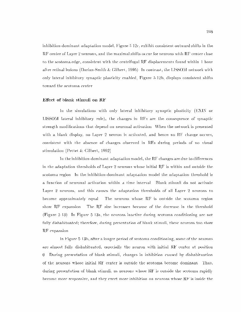
246inhibition-dominant adaptation model, Figure 5.12c, exhibit consistent outward shifts in theRF center of Layer 2 neurons, and the maximal shifts occur for neurons with RF center closeto the scotoma edge, consistent with the centrifugal RF displacements found within 1 hourafter retinal lesions (Darian-Smith & Gilbert, 1995). In contrast, the LISSOM network withonly lateral inhibitory synaptic plasticity enabled, Figure 5.12b, displays consistent shiftstoward the scotoma center.E�ect of blank stimuli on RFIn the simulations with only lateral inhibitory synaptic plasticity (EXIN orLISSOM lateral inhibitory rule), the changes in RFs are the consequence of synapticstrength modi�cations that depend on neuronal activation. When the network is presentedwith a blank display, no Layer 2 neuron is activated, and hence no RF change occurs,consistent with the absence of changes observed in RFs during periods of no visualstimulation (Pettet & Gilbert, 1992).In the inhibition-dominant adaptationmodel, the RF changes are due to di�erencesin the adaptation thresholds of Layer 2 neurons whose initial RF is within and outside thescotoma region. In the inhibition-dominant adaptation model the adaptation threshold isa function of neuronal activation within a time interval. Blank stimuli do not activateLayer 2 neurons, and this causes the adaptation thresholds of all Layer 2 neurons tobecome approximately equal. The neurons whose RF is outside the scotoma regionshow RF expansion. The RF size increases because of the decrease in the threshold(Figure 5.13). In Figure 5.13a, the neurons inactive during scotoma conditioning are notfully dishabituated; therefore, during presentation of blank stimuli, these neurons too showRF expansion.In Figure 5.13b, after a longer period of scotoma conditioning, some of the neuronsare almost fully dishabituated, especially the neuron with initial RF center at position0. During presentation of blank stimuli, changes in inhibition caused by dishabituationof the neurons whose initial RF center is outside the scotoma become dominant. Thus,during presentation of blank stimuli, as neurons whose RF is outside the scotoma rapidlybecome more responsive, and they exert more inhibition on neurons whose RF is inside the

247-14 -12 -10 -8 -6 -4 -2 0 2 4 6 8 10 12 14

-2

-1

0

1

2

EX

IN-L

Iou

twar

din

war

d

scotomareset

(a)

-14 -12 -10 -8 -6 -4 -2 0 2 4 6 8 10 12 14-2

-1

0

1

2

LIS

SO

M-L

Iou

twar

din

war

d

scotomareset

(b)

-14 -12 -10 -8 -6 -4 -2 0 2 4 6 8 10 12 14-2

-1

0

1

2

AN

-ID

Distance from scotoma center

outw

ard

inw

ard

scotomareset

(c)Figure 5.12: RF shift as function of position.Shift in RF center after scotoma conditioning (solid line) and after re-conditioning withnormal stimuli (dashed line) with respect to the initial RF centers is shown as a function ofdistance of the initial RF center of Layer 2 neurons from the scotoma center for the EXINnetwork with only lateral inhibitory synaptic plasticity enabled (a), the LISSOM networkwith only lateral inhibitory synaptic plasticity enabled (b), and the inhibition-dominantadaptation network (c). The RF shift shown is for a one-dimensional cross-section throughLayer 2: neurons (0;�15){(0; 14). Positive and negative shifts represent a shift away fromand toward the center of the scotoma, respectively. The RF center of a Layer 2 neuron isthe center of moment of the neuron's responsiveness to input at di�erent positions withinits RF. See Figure 5.8 for simulation details and conventions.

248scotoma. This results in a slight RF contraction for neurons whose RF is inside the scotoma(Figure 5.13b).Other adaptation modelsXing and Gerstein (1994) measured the initial RFs before conditioning with normalstimuli. Then they conditioned the network using scotoma stimuli. In this case, theneurons in the cortical scotoma region were not a�ected, and those outside the corticalscotoma adapted. Adaptation of the neurons outside the cortical scotoma decreases theirresponsiveness; hence they exert less inhibition on neurons in the cortical scotoma. As aresult, the RFs of the neurons in the scotoma region increased in size and showed otherchanges consistent with experimental data (Figures 5.14{5.17a). However, presenting blankstimuli to the model would result in a decrease in adaptation of all neurons. Thus, the RFswould be restored to their pre-scotoma sizes.Figures 5.14b{c show changes in RF size following arti�cial scotoma conditioningin an adaptation network with no lateral interaction and in an adaptation network withdominant lateral excitation, respectively. The two networks produce RF expansion ininactive neurons after scotoma conditioning, and they produce RF contraction duringnormal stimulation following scotoma conditioning.However, in the adaptation network with no lateral interactions, RF pro�les afterscotoma conditioning are symmetric (Figure 5.15b), and the RF position of the neuronsdo not change (Figure 5.16b). In the adaptation network with dominant lateral excitation,the RF pro�le shows asymmetry, but the neurons are more responsive to locations withinthe occluded region during scotoma conditioning (Figure 5.15c); this manifests itself asRF shifts toward the center of the scotoma (Figure 5.16c). These e�ects are inconsistentwith the observations of Darian-Smith and Gilbert (1995) and Das and Gilbert (1995b).Figures 5.17b{c show that in these adaptation networks, responsiveness returns toneurons within the cortical scotoma in a concentric inward direction.Because the adaptation level in these adaptation models depends on neuronalactivation, the RF size of neurons in these models changes in the absence of inputstimulation.

249

-14 -12 -10 -8 -6 -4 -2 0 2 4 6 8 10 12 140

10

20

30

40

50

60

RF

siz

e (a

rea)

AN

-ID

Distance from scotoma center

after scotoma (15000 steps)after 2500 blanksafter 5000 blanks

(b)

-14 -12 -10 -8 -6 -4 -2 0 2 4 6 8 10 12 140

10

20

30

40

50

60

RF

siz

e (a

rea)

AN

-ID

after scotoma (5000 steps)after 2500 blanksafter 5000 blanks

(a)

Figure 5.13: Simulation results: Blank screen causes RF changes in theinhibition-dominant adaptation model.The RF area after scotoma conditioning (solid line), after 2500 steps of conditioningwith blank stimuli (dashed line), and after 5000 steps of conditioning with blankstimuli (dotted line) in the inhibition-dominant adaptation network after 5000 steps ofscotoma conditioning (a), and after 15000 steps of scotoma conditioning (b), are shown asa function of the position of the initial RF center of Layer 2 neurons relative to the scotomacenter (0; 0). In (a) the neurons in the cortical scotoma were not fully dishabituated andtherefore show RF expansion during no visual stimulation. In (b) prolonged inactivity inneurons in the cortical scotoma causes them to become almost fully dishabituated. Withno visual stimulation, the neurons outside the cortical scotoma are dishabituated and theyexert stronger inhibition on neurons inside the cortical scotoma. Thus, neurons outsidethe cortical scotoma show RF expansion, and neurons inside the cortical scotoma, whichwere highly dishabituated, show RF contraction. See Figure 5.10 for simulation details andconventions.

250-14 -12 -10 -8 -6 -4 -2 0 2 4 6 8 10 12 14

0

30

60

90

120

150

RF

siz

e (a

rea)

AN

-NI

initialduring scotomareset

(b)

-14 -12 -10 -8 -6 -4 -2 0 2 4 6 8 10 12 140

30

60

90

120

RF

siz

e (a

rea)

AN

-ED

Distance from scotoma center

initialduring scotomareset

(c)

-14 -12 -10 -8 -6 -4 -2 0 2 4 6 8 10 12 140

30

60

90

120

RF

siz

e (a

rea)

AN

-ID

(X

G)

initialduring scotomareset

(a)

Figure 5.14: Simulation results: RF size changes in other adaptation models.The RF area before scotoma conditioning (solid line), after scotoma conditioning (dashedline), and after re-conditioning with normal stimuli (dotted line) in the inhibition-dominantadaptation network without prior normal stimulation (a), the adaptation network withoutlateral connections (b), and the excitation-dominant adaptation network (c), are shown asa function of the position of the initial RF center of Layer 2 neurons relative to the scotomacenter (0; 0). In panel (b) the dotted curve overlaps with the solid curve. See Figure 5.9 forsimulation details and conventions.

251-14 -12 -10 -8 -6 -4 -2 0 2 4 6 8 10 12 14

0

5

10

15

20

25

30

Neu

ron

activ

ityA

N-N

I

initialduring scotomareset

(b)

-14 -12 -10 -8 -6 -4 -2 0 2 4 6 8 10 12 140

5

10

15

20

25

30

Neu

ron

activ

ityA

N-E

D

Distance from scotoma center

initialduring scotomareset

(c)

-14 -12 -10 -8 -6 -4 -2 0 2 4 6 8 10 12 140

5

10

15

20

Neu

ron

activ

ityA

N-I

D (

XG

)

initialduring scotomareset

(a)

Figure 5.15: Simulation results: The iceberg e�ect in other adaptation models.Layer 2 neuron responsiveness before scotoma conditioning (solid line), after scotomaconditioning (dashed line), and after re-conditioning with normal stimuli (dotted line)in the inhibition-dominant adaptation network without prior normal stimulation (a), theadaptation network without lateral connections (b), and the excitation-dominant adaptationnetwork (c), are shown as a function of one-dimensional input positions across Layer 1passing through the scotoma center. See Figure 5.8 for simulation details and conventions.

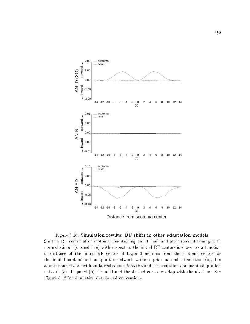
252-14 -12 -10 -8 -6 -4 -2 0 2 4 6 8 10 12 14

-0.01

0.00

0.00

0.00

0.01

AN

-NI

outw

ard

inw

ard

scotomareset

(b)

-14 -12 -10 -8 -6 -4 -2 0 2 4 6 8 10 12 14-0.10

-0.05

0.00

0.05

0.10

AN

-ED

Distance from scotoma center

outw

ard

inw

ard

scotomareset

(c)

-14 -12 -10 -8 -6 -4 -2 0 2 4 6 8 10 12 14-2.00

-1.00

0.00

1.00

2.00

AN

-ID

(X

G)

outw

ard

inw

ard

scotomareset

(a)

Figure 5.16: Simulation results: RF shifts in other adaptation models.Shift in RF center after scotoma conditioning (solid line) and after re-conditioning withnormal stimuli (dashed line) with respect to the initial RF centers is shown as a functionof distance of the initial RF center of Layer 2 neurons from the scotoma center forthe inhibition-dominant adaptation network without prior normal stimulation (a), theadaptation network without lateral connections (b), and the excitation-dominant adaptationnetwork (c). In panel (b) the solid and the dashed curves overlap with the abscissa. SeeFigure 5.12 for simulation details and conventions.

253-14 -12 -10 -8 -6 -4 -2 0 2 4 6 8 10 12 14

0

5

10

15

20

25

30

Neu

ron

activ

ity x

20

AN

-NI

initialafter 2500after 5000

(b)

-14 -12 -10 -8 -6 -4 -2 0 2 4 6 8 10 12 140

5

10

15

20

25

30

Neu

ron

activ

ity x

20

AN

-ED

Distance from scotoma center

initialafter 2500after 5000

(c)

-14 -12 -10 -8 -6 -4 -2 0 2 4 6 8 10 12 140

5

10

15

20

25

30

Neu

ron

activ

ity x

20

AN

-ID

(XG

)

initialafter 2500after 5000

(a)

Figure 5.17: Simulation results: Recovery of responsiveness in other adaptationmodels.The �gures show the activation pattern in Layer 2 in response to input outside the scotomabefore scotoma conditioning (solid line), after 2500 steps of scotoma conditioning (dashedline), and after 5000 steps of scotoma conditioning (dotted line) in the inhibition-dominantadaptation network without prior normal stimulation (a), the adaptation network withoutlateral connections (b), and the excitation-dominant adaptation network (c). The input isa test stimulus centered at Layer 1 neuron (0;�9). See Figure 5.11 for simulation detailsand conventions.

254ConclusionsFrom the simulations presented in this section, it is clear that the LISSOM instarlateral inhibitory synaptic plasticity rule is insu�cient to model the e�ects of arti�cialscotoma conditioning and retinal lesions. However, the EXIN outstar lateral inhibitorysynaptic plasticity rule is su�cient to model these e�ects.Xing and Gerstein's (1994) inhibition-dominant adaptation network failed onlyin modeling the e�ects of presentation of blank stimuli after scotoma conditioning. InSection 5.4, a novel experiment is suggested to determine the role of neuronal adaptationin producing dynamic RF changes that persist over a long periods (about 15 minutes).Cortical neurons are maximally adapted within tens of seconds, and neurons recovertheir responsiveness over a period of tens of seconds (Hammond et al., 1986, 1989).Psychophysical experiments on humans using arti�cial scotoma conditioning produces shiftsin position judgments consistent with the RF expansion hypothesis (Kapadia et al., 1994).These changes occurred over a period of 1-2 seconds, however, and would be consistent withthe inhibition-dominant adaptation model.Thus, we conclude that during scotoma conditioning, e�ects of neuronal adaptationoccur over a period of tens of seconds; however, the persistent e�ects produced over aperiod of 15 minutes to hours may be caused by a long-term process, e.g., long-termsynaptic plasticity. The RF changes observed over a period of months, however, mayinvolve sprouting and establishment of new connections (Darian-Smith & Gilbert, 1994).The issue of time-scales is further discussed in Section 5.5.4.The adaptation models without lateral interaction and with dominant lateralexcitation produced RF expansion in neurons whose RFs were within the scotoma region.However, they produced RF shifts inconsistent with experimental data.Sirosh et al. (1996) explained RF changes during scotoma conditioning using theLISSOM a�erent excitatory synaptic plasticity. However, in their simulations the LISSOMlateral excitatory and lateral inhibitory synaptic plasticity rules were also enabled. To studythe e�ects of a�erent excitatory synaptic plasticity alone during scotoma conditioning, thenext section (Section 5.3.2), presents simulations on the EXIN and LISSOM networks with

255their respective a�erent excitatory synaptic plasticity rules.5.3.2 Role of a�erent excitatory synaptic plasticityIn this section, the e�ects of scotoma conditioning on the EXIN andLISSOM networks with only a�erent excitatory synaptic plasticity enabled are presented.Both the EXIN and LISSOM a�erent excitatory synaptic plasticity rules are instar rules.One di�erence between the two networks is the presence of short-range lateral excitatoryconnections in the LISSOM network.RF size as a function of positionFigures 5.18a{b show the RF size before and after scotoma conditioning as afunction of the position of the initial RF center, for the EXIN and the LISSOM networkswith only a�erent excitatory synaptic plasticity enabled. For the EXIN network with onlya�erent excitatory synaptic plasticity enabled, small RF expansions occurred for Layer 2neurons whose initial RF center is close to and inside the scotoma edge, and Layer 2neurons whose initial RF center is close to and outside the scotoma boundary showedlarger RF contraction (Figure 5.18a). Similarly, the LISSOM network with only a�erentexcitatory synaptic plasticity enabled produced RF expansion in neurons whose initial RF isinside the scotoma and produced RF contraction in neurons close to the scotoma boundary(Figure 5.18b).The EXIN and the LISSOM networks with only a�erent excitatory synapticplasticity enabled produced RF expansion in neurons whose initial RF center is insidethe scotoma, consistent with the results of Pettet and Gilbert (1992).The LISSOM network with a�erent excitatory synaptic plasticity alone showedlarger RF expansion than the EXIN network with only a�erent excitatory synaptic plasticityenabled because of the short-range lateral excitatory connections in the LISSOM network.In the LISSOM network, the neurons whose responsiveness increased (because of decreasedinhibition through weakening of a�erent pathways converging on other neurons) elevatedthe responsiveness of their neighbors via lateral excitatory connections, thereby producinglarge RF expansions. In Figure 5.18b, the curve showing RF size after scotoma conditioning

256-14 -12 -10 -8 -6 -4 -2 0 2 4 6 8 10 12 14

0

10

20

30

40

50

60

70

RF

siz

e (a

rea)

EX

IN-F

F

initialduring scotomareset

(a)

-14 -12 -10 -8 -6 -4 -2 0 2 4 6 8 10 12 140

10

20

30

40

50

60

70

RF

siz

e (a

rea)

EX

IN-L

I+F

F

Distance from scotoma center

initialduring scotomareset

(c)

-14 -12 -10 -8 -6 -4 -2 0 2 4 6 8 10 12 140102030405060708090

100

RF

siz

e (a

rea)

LIS

SO

M-F

F

initialduring scotomareset

(b)

Figure 5.18: Simulation results: RF size changes caused by a�erent excitatoryplasticity.The RF area before scotoma conditioning (solid line), after scotoma conditioning (dashedline), and after re-conditioning with normal stimuli (dotted line) in the EXIN network withonly a�erent excitatory synaptic plasticity enabled (a), the LISSOM network with onlya�erent excitatory synaptic plasticity enabled (b), and the EXIN network with a�erentexcitatory and lateral inhibitory synaptic plasticity (c), are shown as a function of theposition of the RF center of Layer 2 neurons relative to the scotoma center (0; 0). SeeFigure 5.9 for conventions and simulation details.

257is unimodal. The curve would become bimodal when the scotoma size is increased. In theLISSOM network, the weight of the lateral excitatory and inhibitory pathway decreases asthe distance between the source and target neurons increases. Thus, as the scotoma sizeis increased, the e�ects of lateral pathways between neurons whose RFs are close to thescotoma boundary and neurons whose RFs are close to the center of the scotoma decrease,and therefore the amount of RF expansion in neurons whose RFs are close to the scotomacenter will be less than the amount of RF expansion in neurons whose RFs are inside thescotoma, but closer to the scotoma boundary than the scotoma center. Thus, the RF sizecurve after scotoma conditioning becomes bimodal.Figure 5.19 shows the RF pro�le of a neuron that exhibited RF expansion andanother that exhibited RF contraction in the two simulations. After scotoma conditioning,the RF pro�le of some neurons in these networks was asymmetric, consistent withobservations of Das and Gilbert (1995b). The asymmetric RF shape is caused by asymmetricchanges in weights in the two networks.In Figure 5.18a, neurons far away from the scotoma showed RF expansion.In the EXIN network with only a�erent excitatory synaptic plasticity enabled, duringscotoma conditioning neurons initially in the cortical scotoma strengthened their a�erentconnections from locations outside the scotoma. Thus, neurons surrounding the corticalscotoma received more inhibition when locations outside the scotoma were stimulated, andsuppression of responsiveness of these neurons resulted in a slight increase in responsivenessof neurons farther away from the scotoma (Figure 5.20).Recovery of neurons in the cortical scotomaThe EXIN and the LISSOM networks with only a�erent excitatory synapticplasticity enabled exhibited new responsiveness to stimuli outside the scotoma in neuronswhose initial RF is inside the scotoma, during scotoma conditioning (Figure 5.21). This isconsistent with the �nding that after bilateral retinal lesions, function returned over timeto the cortex in a roughly concentric inward direction (Darian-Smith & Gilbert, 1995).

258-14 -12 -10 -8 -6 -4 -2 0 2 4 6 8 10 12 14

0

4

8

Neu

ron

activ

ityE

XIN

-FF

initialduring scotomareset

(a)

-14 -12 -10 -8 -6 -4 -2 0 2 4 6 8 10 12 140

4

8

Neu

ron

activ

ityE

XIN

-FF

initialduring scotomareset

(b)

-14 -12 -10 -8 -6 -4 -2 0 2 4 6 8 10 12 140

4

8

Neu

ron

activ

ityLI

SS

OM

-FF

initialduring scotomareset

(c)

-14 -12 -10 -8 -6 -4 -2 0 2 4 6 8 10 12 140

4

8

Neu

ron

activ

ityLI

SS

OM

-FF

Distance from scotoma center

initialduring scotomareset

(d)Figure 5.19: Simulation results: RF pro�les of neurons that show expansion orcontraction.Layer 2 neuron RF pro�les before scotoma conditioning (solid line), after scotomaconditioning (dashed line), and after re-conditioning with normal stimuli (dotted line)in the EXIN network with only a�erent excitatory synaptic plasticity enabled (a,b), andthe LISSOM network with only a�erent excitatory synaptic plasticity enabled (c,d), as afunction of a one-dimensional input positions across Layer 1 passing through the scotomacenter. In (a) and (c), the neurons show RF expansion, and in (b) and (d), the neurons showRF contraction. See Figure 5.8 for simulation details and conventions. The thick line on theabscissa represents the scotoma region. In (a) and (c), the neurons showed RF expansion,and in (b) and (d) the neurons showed RF contraction.

259-14 -12 -10 -8 -6 -4 -2 0 2 4 6 8 10 12 14

048121620

Neu

ron

activ

ityE

XIN

-FF

initialafter 25000after 50000

(a)

-14 -12 -10 -8 -6 -4 -2 0 2 4 6 8 10 12 14048121620

Neu

ron

activ

ityE

XIN

-FF

initialafter 25000after 50000

(b)

-14 -12 -10 -8 -6 -4 -2 0 2 4 6 8 10 12 14048

121620

Neu

ron

activ

ityE

XIN

-FF

initialafter 25000after 50000

(c)

-14 -12 -10 -8 -6 -4 -2 0 2 4 6 8 10 12 14048

121620

Neu

ron

activ

ityE

XIN

-FF

Distance from scotoma center

initialafter 25000after 50000

(d)Figure 5.20: Simulation results: Activation pro�les in response to inputs atlocations away from the scotoma.The �gure shows activation of a one-dimensional cross-section ofLayer 2 neurons: (0;�15){(0; 14), in response to input stimulation at (0; 11) (a), (0; 12) (b),(0; 13) (c), and (0; 14) (d) in the EXIN network with only a�erent excitatory synapticplasticity enabled. The activation level of the neurons was scaled by a factor of 20. SeeFigure 5.11 for conventions and simulation details.

260-14 -12 -10 -8 -6 -4 -2 0 2 4 6 8 10 12 14

02468101214161820

Neu

ron

activ

ity x

20

EX

IN-F

F

initialafter 25000after 50000

(a)

-14 -12 -10 -8 -6 -4 -2 0 2 4 6 8 10 12 1402468101214161820

Neu

ron

activ

ity x

20

LIS

SO

M-F

F

Distance from scotoma center

initialafter 2500after 5000

(b)Figure 5.21: Simulation results: Recovery of responsiveness of Layer 2 neuronscaused by a�erent excitatory plasticity.The �gures show the activation pattern in Layer 2 in response to input outside the scotomabefore scotoma conditioning (solid line), after 2500 steps of scotoma conditioning (dashedline), and after 5000 steps of scotoma conditioning (dotted line) in the EXIN network withonly a�erent excitatory synaptic plasticity enabled (a) and the LISSOM network with onlya�erent excitatory synaptic plasticity enabled (b). See Figure 5.11 for conventions andsimulation details.

261RF shiftsFigures 5.22a{b display the shift in RF center after conditioning with scotomastimuli as a function of the position of the initial RF center of each Layer 2 neuron.The EXIN and LISSOM networks with only a�erent excitatory synaptic plasticity enabled,Figures 5.22a{b, exhibited consistent outward shifts in the RF center of Layer 2 neurons.The maximal shifts occurred for neurons whose RF center was close to the scotoma edge.These results are consistent with the consistent small centrifugal RF shift away from thelesion center, between �ve minutes and one hour after the retinal lesions, observed byDarian-Smith and Gilbert (1995). In the two networks, neurons whose initial RF centerwas inside the scotoma showed outward shift because of the asymmetric RF expansion(Figure 5.19), and neurons whose initial RF overlapped the scotoma boundary showed anoutward shift because of RF contraction (Figure 5.19).During normal stimulation following scotoma conditioning, the EXIN networkwith only a�erent excitatory synaptic plasticity enabled did not recover (Figure 5.22a).This e�ect was caused by strong lateral inhibition, which prevented the neurons whoseRF size decreased (because of weakening of pathways from the scotoma during scotomaconditioning) from becoming strongly active to inputs at positions inside the scotoma.The weak a�erent connections were thus prevented from becoming strong. In the LISSOMnetwork with a�erent excitatory synaptic plasticity alone, the short-range lateral excitatoryconnections helped neurons with weak a�erent connections from the scotoma region tobecome more active, and hence to strengthen the weak a�erent pathways (Figure 5.22b).To ensure that the lack of recovery in the EXIN simulation was not causedby insu�cient training, the simulation was run for much longer time (dotted line inFigure 5.22a). In fact, additional training shifted the RFs of neurons farther away fromtheir original positions. The dotted line in Figure 5.22a is jagged, implying that theRF positions of some neurons shifted toward the scotoma center and the RF positions ofneighboring neurons shifted away from the scotoma center. This behavior is the consequenceof the strong lateral inhibitory interactions between the neurons. Because of stronglateral inhibition, when a neuron's responsiveness increases it suppresses the activation

262-14 -12 -10 -8 -6 -4 -2 0 2 4 6 8 10 12 14

-3

-2

-1

0

1

2

3

EX

IN-F

Fou

twar

din

war

d

scotomareset (50000)reset (100000)

(a)

-14 -12 -10 -8 -6 -4 -2 0 2 4 6 8 10 12 14-3

-2

-1

0

1

2

3

EX

IN-L

I+F

F

Distance from scotoma center

outw

ard

inw

ard

scotomareset (50000)reset (100000)

(c)

-14 -12 -10 -8 -6 -4 -2 0 2 4 6 8 10 12 14-3

-2

-1

0

1

2

3

LIS

SO

M-F

Fou

twar

din

war

d

scotomareset (5000)reset (10000)

(b)

Figure 5.22: Simulation results: RF shifts caused by a�erent excitatory plasticity.Shift in RF center after scotoma conditioning (solid line), after re-conditioning withnormal stimuli for 50,000 steps (dashed line), and after re-conditioning with normal stimulifor 100,000 steps (dotted line) with respect to the initial RF centers is shown as a functionof distance of the initial RF center of Layer 2 neurons from the scotoma center for the EXINnetwork with only a�erent excitatory synaptic plasticity enabled (a), the LISSOM networkwith only a�erent excitatory synaptic plasticity enabled (b), and the EXIN network withboth a�erent excitatory and lateral inhibitory synaptic plasticity (c). See Figure 5.12 forconventions and simulation details.

263of neighboring neurons, and thus neurons farther away from the neighbor neurons receiveless inhibition. This alternation of increased inhibition and decreased inhibition causesRF shifts in opposite directions in neighboring neurons.However, with both the a�erent excitatory and the lateral inhibitory synapticplasticity enabled, the neurons in the EXIN network tended to recover their originalRF properties (size, position, shape, and responsiveness) during normal stimulationfollowing scotoma conditioning. During normal stimulation following scotoma conditioning,lateral inhibitory connection weights to the weakly active neurons decreased, and lateralinhibitory connection weights to strongly neurons increased. This led to an attractione�ect on neurons with weakened a�erent connections from the scotoma region and arepulsive e�ect on neurons with strengthened a�erent connections from outside the scotomaregion, resulting in a shift in RF centers toward their original locations (Figure 5.22c) andrestoration of the original RF sizes (Figure 5.18c). During the normal stimulation followingscotoma conditioning, the EXIN network with only lateral inhibitory synaptic plasticity rulecompletely recovered the original RF properties, but the EXIN network with only a�erentexcitatory synaptic plasticity enabled did not recover the original RF properties. Thus, inthe full EXIN network, the amount of recovery of RF properties during normal stimulationfollowing scotoma conditioning will depend on which rule produces the dominant e�ects.E�ect of blank stimuli on RFsIn the EXIN and LISSOM networks with a�erent excitatory synaptic plasticityalone, a blank input display causes the Layer 2 neurons to be inactive, and therefore a�erentexcitatory pathway weights and cortical RFs do not change.ConclusionsThe EXIN and the LISSOM networks with only a�erent excitatory synapticplasticity enabled produced RF expansion consistent with experimental e�ects of arti�cialscotoma conditioning and bilateral retinal lesions. The EXIN network with only a�erentexcitatory synaptic plasticity enabled did not recover during normal stimulation followingscotoma conditioning. However, the full EXIN network with both a�erent excitatory and

264lateral inhibitory synaptic plasticity enabled, did recover. In both the EXIN and theLISSOM networks with only a�erent excitatory synaptic plasticity enabled, RF contractionin neurons whose initial RF overlapped the scotoma edge was observed during scotomaconditioning.5.3.3 Role of lateral excitatory synaptic plasticityIn this section, the e�ects of the LISSOM instar lateral excitatory synapticplasticity rule alone during scotoma conditioning are presented.These simulations demonstrate that in a network with short-range lateral dominantexcitatory connections and long-range lateral dominant inhibitory connections, an instarrule to modify the short-range lateral excitatory connections during scotoma conditioningproduces RF expansion in neurons whose initial RF center is inside the scotoma.RF size as a function of positionFigure 5.23a shows the RF size before and after scotoma stimuli conditioning as afunction of the position of the initial RF center. In the LISSOM network with only instarlateral excitatory synaptic plasticity enabled, Figure 5.23a, RF expansions occurred forLayer 2 neurons whose initial RF center is inside the scotoma edge. In addition, neuronswhose initial RF center is close to and outside the scotoma boundary showed RF contraction.These e�ects are similar to those observed in the EXIN and the LISSOM networks withonly a�erent excitatory synaptic plasticity enabled (Section 5.3.2).In the LISSOM network with instar lateral excitatory synaptic plasticity alone,during scotoma conditioning the lateral excitatory pathways from the neurons just insidethe cortical scotoma to those just outside weaken. Thus, in the LISSOM network withonly instar lateral excitatory synaptic plasticity enabled, neurons whose RF is close to andoutside the scotoma become less responsive to stimulation within and close to the scotomaboundary. This causes RF contraction in neurons whose initial RF is close to and outsidethe scotoma. Furthermore, because of the decreased responsiveness of these neurons tostimulation within and close to the scotoma boundary, they exert less inhibition on neuronswhose initial RF is inside and away from the scotoma boundary, resulting in RF expansion.

265-14 -12 -10 -8 -6 -4 -2 0 2 4 6 8 10 12 14

0

10

20

30

40

50

60

70

RF

siz

e (a

rea)

LIS

SO

M-L

E

initialduring scotomareset

(a)

-14 -12 -10 -8 -6 -4 -2 0 2 4 6 8 10 12 140

1

2

3

4

5

Neu

ron

activ

ityLI

SS

OM

-LE

initialduring scotomareset

(b)

-14 -12 -10 -8 -6 -4 -2 0 2 4 6 8 10 12 1402468101214161820

Neu

ron

activ

ity x

20

LIS

SO

M-L

E

initialafter 12500after 25000

(c)

-14 -12 -10 -8 -6 -4 -2 0 2 4 6 8 10 12 14-2

-1

0

1

2

LIS

SO

M-L

Eou

twar

din

war

d

scotomareset

(d)Figure 5.23: Legend on next page.

266Figure 5.23: Simulation results: RF changes in the LISSOM network with onlylateral excitatory plasticity enabled.Figure on previous page. (a) The RF area before scotoma conditioning (solid line), afterscotoma conditioning (dashed line), and after re-conditioning with normal stimuli (dottedline), is shown as a function of the position of the initial RF center of Layer 2 neuronsrelative to the scotoma center (0; 0). See Figure 5.9 for conventions and simulation details.(b) Layer 2 neuron responsiveness before scotoma conditioning (solid line), after scotomaconditioning (dashed line), and after re-conditioning with normal stimuli (dotted line), areshown as a function of one-dimensional input positions across Layer 1 passing throughthe scotoma center. See Figure 5.8 for conventions and simulation details. (c) Theactivation pattern in Layer 2 in response to input outside the scotoma before scotomaconditioning (solid line), after 2,500 steps of scotoma conditioning (dashed line), andafter 5,000 steps of scotoma conditioning (dotted line). The input is a test stimuluscentered at Layer 1 neuron (0;�9). (d) Shift in RF center after scotoma conditioning (solidline) and after re-conditioning with normal stimuli (dashed line) with respect to the initialRF centers is shown as a function of distance of Layer 2 neurons from the scotoma center.See Figure 5.12 for conventions and simulation details.In Figure 5.23b, the neuron became more responsive to locations away from thescotoma center, consistent with the results of Das and Gilbert (1995b). Normal stimulationfollowing scotoma conditioning restored the RF size in the LISSOM network with instarexcitatory synaptic plasticity alone (Figure 5.23).Recovery of neurons in the cortical scotomaThe LISSOM network with instar lateral excitatory synaptic plasticity aloneexhibited new responsiveness to stimuli outside the scotoma in neurons whose initial RF isinside the scotoma, during scotoma conditioning (Figure 5.23c).RF shiftsFigure 5.23d displays the shift in RF center after conditioning with scotoma stimulias a function of the initial RF center position of Layer 2 neurons. The LISSOM networkwith only instar lateral excitatory synaptic plasticity enabled exhibits consistent outwardshifts (Figure 5.23d).In the LISSOM network with only instar lateral excitatory synaptic plasticity

267enabled, neurons whose initial RF center is inside the scotoma showed outward shift becauseof asymmetric RF expansion (Figure 5.23b), and neurons whose initial RF overlapped thescotoma boundary showed outward shift because of RF contraction.E�ect of blank stimuli on RFIn the LISSOM network with only lateral excitatory synaptic plasticity enabled,when no input stimulation is present, Layer 2 neurons are inactive, and therefore lateralexcitatory pathway weights and cortical RFs do not change.ConclusionsThe LISSOM network with instar lateral excitatory synaptic plasticity aloneproduces many e�ects consistent with the experimental e�ects of arti�cial scotomaconditioning and bilateral retinal lesions. The LISSOM network with only instar lateralexcitatory synaptic plasticity enabled produces RF contraction in neurons whose initial RFis just outside the scotoma during scotoma conditioning. Instar lateral excitatorysynaptic plasticity in a network with short-range lateral excitatory connections and long-range inhibitory connections thus models dynamic RF changes during arti�cial scotomaconditioning.In the LISSOM network, if the outstar lateral excitatory synaptic plasticity ruleis used instead of the LISSOM instar lateral excitatory synaptic plasticity rule, then afterscotoma conditioning the network may produce RF expansion in neurons outside the corticalscotoma and may produce RF shifts toward the scotoma center. These may happen duringscotoma conditioning because an outstar lateral excitatory synaptic plasticity rule weakenslateral excitatory pathways from active neurons to inactive neurons, whereas an instarlateral excitatory synaptic plasticity rule weakens lateral excitatory pathways from inactiveneurons to active neurons.

2685.4 Simulation results: Complementary scotoma stimuliThe EXIN network (with a�erent excitatory synaptic plasticity or lateralinhibitory synaptic plasticity alone), the LISSOM network (with a�erent excitatory synapticplasticity or instar lateral excitatory synaptic plasticity alone), and the inhibition-dominantadaptation model explain many important features of the arti�cial scotoma experiment(Pettet & Gilbert, 1992) and the experiment on the short-term e�ects of the bilateral retinallesion (Darian-Smith & Gilbert, 1995). However, the inhibition-dominant adaptation modeldi�ers from other models in its behavior after blank screen conditioning (Section 5.3.1). TheEXIN network with instar a�erent excitatory synaptic plasticity alone and the LISSOMnetwork with instar a�erent or instar lateral excitatory synaptic plasticity alone produceRF contraction during scotoma conditioning, in neurons whose initial RF overlaps thescotoma boundary.To further distinguish between the EXIN synaptic plasticity rules, the LISSOMsynaptic plasticity rules, and the adaptation rule, a \complementary scotoma" stimulationexperiment is proposed. In this conditioning paradigm, after the initial conditioningwith normal stimuli, the network is presented with stimuli that have two alternating,complementary scotoma regions. That is, for any stimulus, the scotoma is a hemi�eldor its complementary hemi�eld. The duration of presentation, inter-trial interval, andduration before testing after conditioning should be varied to control for the ubiquitousneuronal adaptation in the cortex. The duration of presentation of each hemi�eld shouldshort (e.g., 1{10 seconds).5.4.1 RF changes because of synaptic plasticityIn the EXIN network with only lateral inhibitory synaptic plasticity enabled,neurons whose RF is near the common boundary of the complementary scotoma regionsshow maximal increase in RF size. The expansion is due to the decrease in thelateral inhibitory weights between layer 2 neurons whose RFs are inside and outsidethe common boundary of the complementary scotoma regions. The decrease occursbecause these neurons are never coactivated during complementary scotoma conditioning.

269Figure 5.24a shows the results of a complementary scotoma simulation, plotting Layer 2RF size as a function of position of the initial RF center. The RF expansion wasaccompanied by an increase in responsiveness of the corresponding Layer 2 neurons.Figure 5.24b shows Layer 2 RF size as a function of position of the initial RF center,after the LISSOM network with only lateral inhibitory synaptic plasticity enabled waspresented with complementary scotoma stimuli. The behavior of the LISSOM network withonly lateral inhibitory synaptic plasticity enabled was similar to that of the EXIN networkwith only lateral inhibitory synaptic plasticity enabled for this conditioning. Layer 2neurons in the LISSOM network, with RFs inside and outside the common boundary ofthe complementary scotoma regions, were never coactivated. This resulted in a decrease inthe strength of lateral inhibitory connections between these neurons. Thus, RFs near theboundary increased in size.Figure 5.25a shows Layer 2 RF size as a function of position of the initial RF centerafter the EXIN network with only a�erent excitatory synaptic plasticity enabled waspresented with complementary scotoma stimuli. The neurons whose initial RF overlappedthe complementary scotoma boundary showed RF contraction, as these neurons receivedweakened a�erent pathways from positions close to the complementary scotoma boundary.Complementary scotoma conditioning of the LISSOM network with only a�erent excitatorysynaptic plasticity enabled produced the same e�ects (Figure 5.25b).The LISSOM network with instar lateral excitatory synaptic plasticity aloneproduced RF contraction in neurons whose initial RF straddled the complementary scotomaboundary. This happens because anti-correlated activity in neurons whose initial RF centerlay on opposite sides of the complementary scotoma boundary results in weakening of mutuallateral excitatory connections, leading to RF contraction (Figure 5.25c).In the EXIN and the LISSOM networks with only lateral inhibitory synapticplasticity enabled, the RFs of neurons across the complementary scotoma boundary shiftedtoward each other (Figure 5.26). However, in the EXIN network with only a�erentexcitatory plasticity enabled and in the LISSOM network with either a�erent excitatory orlateral excitatory plasticity enabled, the RFs of neurons across the complementary scotomaboundary shifted away from each other (Figure 5.27). In the LISSOM network with lateral

270-14 -12 -10 -8 -6 -4 -2 0 2 4 6 8 10 12 14

0

10

20

30

40

RF

siz

e (a

rea)

EX

IN-L

I

initialduring scotomareset

(a)

-14 -12 -10 -8 -6 -4 -2 0 2 4 6 8 10 12 1440

50

60

70

80

RF

siz

e (a

rea)

LIS

SO

M-L

I

initialduring scotomareset

(b)

-14 -12 -10 -8 -6 -4 -2 0 2 4 6 8 10 12 1420

21

22

23

24

25

RF

siz

e (a

rea)

AN

-ID

Distance from scotoma center

initialduring scotomareset

(c)Figure 5.24: Simulation results: Average RF size changes after complementaryscotoma conditioning.The average RF area before complementary scotoma conditioning (solid line), aftercomplementary scotoma conditioning (dashed line), and after re-conditioning with normalstimuli (dotted line) in the EXIN network with only lateral inhibitory synaptic plasticityenabled (a), the LISSOM network with only lateral inhibitory synaptic plasticityenabled (b), and the inhibition-dominant adaptation network (c), are shown as a functionof the position of the initial RF center of Layer 2 neurons relative to the scotoma center.The scotoma is a hemi�eld of size 15� 30. The average RF area shown at each position isthe mean over the RF area of neurons with same x coordinate. The RF area of a Layer 2neuron is de�ned as the number of locations at which the test stimulus evokes a response inthe Layer 2 neuron. In panel (c) the dotted curve overlaps with the solid curve. The thickline segment on the abscissa represents the scotoma region.

271-14 -12 -10 -8 -6 -4 -2 0 2 4 6 8 10 12 14

0

10

20

30

40

RF

siz

e (a

rea)

EX

IN-F

F

initialduring scotomareset

(a)

-14 -12 -10 -8 -6 -4 -2 0 2 4 6 8 10 12 1440

50

60

70

80

RF

siz

e (a

rea)

LIS

SO

M-F

F

initialduring scotomareset

(b)

-14 -12 -10 -8 -6 -4 -2 0 2 4 6 8 10 12 145051525354555657585960

RF

siz

e (a

rea)

LIS

SO

M-L

E

initialduring scotomareset

(c)Figure 5.25: Simulation results: Average RF size changes after complementaryscotoma conditioning.The average RF area before complementary scotoma conditioning (solid line), aftercomplementary scotoma conditioning (dashed line), and after re-conditioning with normalstimuli (dotted line) in the EXIN network with only a�erent excitatory synaptic plasticityenabled (a), the LISSOM network with only a�erent excitatory synaptic plasticityenabled (b), and the LISSOM network with only instar lateral excitatory synaptic plasticityenabled (c), are shown as a function of the position of the initial RF center of Layer 2 neuronsrelative to the scotoma center. See Figure 5.24 for conventions and simulation details.

272excitatory plasticity alone, smaller RF shifts in neurons far from the cortical complementaryscotoma boundary were due to reduced inhibition to these neurons from neurons close tothe cortical complementary scotoma boundary.5.4.2 RF changes because of neuronal adaptationDuring complementary scotoma conditioning, Layer 2 neurons are activatedalternately because of the alternate complementary input stimulations. Thus, Layer 2neurons become less adapted compared to the adaptation level after the initial whole �eldstimulation.In the computer simulations of complementary scotoma conditioning of theinhibition-dominant network, Layer 2 neurons whose initial RF straddles the complementaryscotoma boundary were more adapted than neurons whose initial RF is away from thecomplementary scotoma boundary. But the Layer 2 RF size as a function of the initialRF center position was almost at (Figure 5.24c). Note that the RF size of a Layer 2neuron was de�ned as the number of input positions at which stimulation drives theneuron's activation above a threshold. The di�erence in adaptation level among the neuronswas not large enough to produce signi�cant change in RF size. The small di�erences inthe adaptation level of Layer 2 neurons after complementary scotoma conditioning wasmanifested as small RF shifts (Figure 5.26c). Because neurons whose RF center wasclose to the complementary scotoma boundary were more adapted than the other neurons,they exerted less lateral inhibition on neurons whose initial RF center was away from thecomplementary scotoma boundary, and the RF center of neurons whose RF center was oneither side of the complementary scotoma boundary shifted toward each other. If neuronswhose RF center was close to the complementary scotoma boundary were less adapted thanthe other neurons, then they would have maximal RF size, and they would exert morelateral inhibition on neurons whose initial RF center was away from the complementaryscotoma boundary; thus the RF centers of neurons whose RF centers were on either side ofthe complementary scotoma boundary would shift away from each other.In the simulation of complementary scotoma conditioning of the adaptationnetwork with no lateral interaction, Layer 2 neurons whose RF center was close to the

273-14 -12 -10 -8 -6 -4 -2 0 2 4 6 8 10 12 14

-0.50

-0.25

0.00

0.25

0.50

EX

IN-L

Iou

twar

din

war

d

scotomareset

(a)

-14 -12 -10 -8 -6 -4 -2 0 2 4 6 8 10 12 14-0.50

-0.25

0.00

0.25

0.50

LIS

SO

M-L

Iou

twar

din

war

d

scotomareset

(b)

-14 -12 -10 -8 -6 -4 -2 0 2 4 6 8 10 12 14-0.10

-0.05

0.00

0.05

0.10

AN

-ID

Distance from scotoma center

outw

ard

inw

ard

scotomareset

(c)Figure 5.26: Simulation results: Average RF shifts after complementary scotomaconditioning.The average shift in the RF center after complementary scotoma conditioning (solid line)and after re-conditioning with normal stimuli (dashed line) with respect to the initialRF centers is shown as a function of distance of the initial RF center of Layer 2 neuronsfrom the scotoma center for the EXIN network with only lateral inhibitory synapticplasticity enabled (a), the LISSOM network with only lateral excitatory synaptic plasticityenabled (b), and the adaptation network (c). The average RF shift shown at each positionis the mean over the shift in RF center of neurons with same x coordinate. Positiveand negative shifts represent a shift away from and toward the center of the scotoma,respectively. The RF center of a Layer 2 neuron is the center of moment of the neuron'sresponsiveness to input at di�erent positions within its RF. See Figure 5.24 for simulationdetails and conventions.

274-14 -12 -10 -8 -6 -4 -2 0 2 4 6 8 10 12 14

-1.00

-0.50

0.00

0.50

1.00

EX

IN-F

Fou

twar

din

war

d

scotomareset

(a)

-14 -12 -10 -8 -6 -4 -2 0 2 4 6 8 10 12 14-1.00

-0.50

0.00

0.50

1.00

LIS

SO

M-F

Fou

twar

din

war

d

scotomareset

(b)

-14 -12 -10 -8 -6 -4 -2 0 2 4 6 8 10 12 14-1.00

-0.50

0.00

0.50

1.00

LIS

SO

M-L

Eou

twar

din

war

d

scotomareset

(c)Figure 5.27: Simulation results: Average RF shifts after complementary scotomaconditioning.The average shift in the RF center after complementary scotoma conditioning (solid line)and after re-conditioning with normal stimuli (dashed line) with respect to the initialRF centers is shown as a function of distance of the initial RF center of Layer 2 neuronsfrom the scotoma center for the EXIN network with only a�erent excitatory synapticplasticity enabled (a), the LISSOM network with only a�erent excitatory synaptic plasticityenabled (b), and and the LISSOM network with only instar lateral excitatory synapticplasticity enabled (c). See Figure 5.26 for conventions.

275-14 -12 -10 -8 -6 -4 -2 0 2 4 6 8 10 12 14

80

90

100

110

RF

siz

e (a

rea)

AN

-NI

initialduring scotomareset

(a)

-14 -12 -10 -8 -6 -4 -2 0 2 4 6 8 10 12 140

10

20

30

40

50

60

RF

siz

e (a

rea)

AN

-ED

Distance from scotoma center

initialduring scotomareset

(b)Figure 5.28: Simulation results: Average RF size changes after complementaryscotoma conditioning.The average RF area before complementary scotoma conditioning (solid line), aftercomplementary scotoma conditioning (dashed line), and after re-conditioning with normalstimuli (dotted line) in the adaptation network with no lateral interaction (a), and in theexcitation-dominant adaptation network (b), are shown as a function of the position of theinitial RF center of Layer 2 neurons relative to the scotoma center. In panels (a,b) thedotted curve overlaps with the solid curve. See Figure 5.24 for conventions and simulationdetails.complementary scotoma boundary were more adapted than other neurons. Thus, they mayhave a smaller RF than neurons whose initial RF center was away from the complementaryscotoma boundary. As in the simulation of the inhibition-dominant adaptation model, theRF sizes of Layer 2 neurons were almost the same (Figure 5.28a). No RF shifts occurredbecause there are no lateral interactions (Figure 5.29a). If Layer 2 neurons whose RF centerwas close to the complementary scotoma were less adapted than other neurons, they wouldhave larger RFs than other neurons, and again there would not be any RF shifts.In the simulation of complementary scotoma conditioning of the

276-14 -12 -10 -8 -6 -4 -2 0 2 4 6 8 10 12 14

-0.02

-0.01

0.00

0.01

0.02

AN

-NI

outw

ard

inw

ard

scotomareset

(a)

-14 -12 -10 -8 -6 -4 -2 0 2 4 6 8 10 12 14-0.02

-0.01

0.00

0.01

0.02

AN

-ED

Distance from scotoma center

outw

ard

inw

ard

scotomareset

(b)Figure 5.29: Simulation results: Average RF shifts after complementary scotomaconditioning.The average shift in the RF center after complementary scotoma conditioning (solid line)and after re-conditioning with normal stimuli (dashed line) with respect to the initialRF centers is shown as a function of distance of the initial RF center of Layer 2 neuronsfrom the scotoma center for the adaptation network with no lateral interaction (a) and forthe excitation-dominant adaptation network (b). In panel (a) the solid and dashed curvesoverlap with the abscissa because there were no RF shifts. See Figure 5.26 for conventions.excitation-dominant adaptation, Layer 2 neurons whose RF center was close to thecomplementary scotoma boundary were less adapted than other neurons. Thus, they hadlarger RFs than neurons whose initial RF center was away from the complementary scotomaboundary (Figure 5.28b). Because neurons whose RF center was close to the complementaryscotoma boundary were less adapted than the other neurons, they exerted more lateralexcitation on neurons whose initial RF center was away from the complementary scotomaboundary, and the RF centers of neurons whose RF centers were on either side of thecomplementary scotoma boundary shifted toward each other (Figure 5.29b). If neurons

277whose RF center was close to the complementary scotoma boundary were more adaptedthan the other neurons, then they would have smaller RFs than other neurons, and theywould exert less lateral excitation on neurons whose initial RF center was away from thecomplementary scotoma boundary; thus, the RF centers of neurons whose RF centers wereon either side of the complementary scotoma boundary would shift away from each other.E�ects of network interactions on neuronal adaptationIn the adaptation networks, the complementary scotoma stimulation activatesLayer 2 neurons with close to equal probability. The adaptation levels of Layer 2 neuronsin the adaptation networks are not necessarily equal for the following reasons. (1) Neuronswhose initial RF straddles the complementary scotoma boundary are activated slightlymore often (although possibly at a lower intensity), and therefore these neurons may becomeslightly more adapted than other neurons. (2) Neurons whose RF center is close to the centerof a hemi�eld have a large number of their a�erent excitatory pathways excited when thathemi�eld is stimulated, whereas neurons whose RF center is close to the complementaryscotoma boundary have only a small number of their a�erent excitatory pathways excited.Thus, neurons whose RF center is close to the center of a hemi�eld are likely to be morestrongly activated and therefore more adapted than neurons whose RF center is close to thecomplementary scotoma boundary. (3) The di�erence in the amount of a�erent excitationreceived by the Layer 2 neurons is further accentuated by the adaptation threshold. IfLayer 2 neurons have large thresholds, neurons receiving larger a�erent excitation are morelikely to be activated and hence be more adapted. (4) In the inhibition-dominant adaptationnetwork, neurons whose RF center is close to the complementary scotoma boundary receiveless lateral inhibition than neurons whose RF center is close to the center of a hemi�eld, thusmaking neurons whose RF center is close to the complementary scotoma boundary likely torespond strongly and become more adapted. On the other hand, in the excitation-dominantadaptation network, neurons whose RF center is close to the complementary scotomaboundary receive less lateral excitation than neurons whose RF center is close to the centerof a hemi�eld, thus making them respond weakly and become less adapted. The eventualdistribution of adaptation levels will be determined by the more dominant factors.

2785.4.3 Recovery of RF propertiesNormal stimulation following complementary scotoma conditioning causedrestoration of the original RF size and position in the EXIN and LISSOM networks withonly lateral inhibitory synaptic plasticity enabled, in all the adaptation networks, and inthe LISSOM network with only a�erent synaptic plasticity enabled (Figures 5.24{5.29).The EXIN network with only a�erent excitatory synaptic plasticity enabled(Figures 5.25a and 5.27a) did not recover its original RF properties. The LISSOM networkwith only lateral excitatory synaptic plasticity enabled (Figures 5.25c and 5.27c) also didnot recover some of its original RF properties, because as the lateral excitatory pathwaysweaken, e�ective inhibition between neurons increases, and increased lateral inhibitionmakes Layer 2 neurons less coactive.5.4.4 ConclusionsComplementary scotoma conditioning revealed di�erences in the behaviors ofthe various models. Thus, a neurobiological experiment using complementary scotomaconditioning could discriminate between the di�erent models based on their predictions.The predictions of the di�erent models are described below.After complementary scotoma conditioning, the EXIN and the LISSOM network,with only their respective lateral inhibitory synaptic plasticity rules enabled, predictthat cortical neurons whose initial RF centers were close to the complementary scotomaboundary would have larger RFs than neurons whose initial RF centers were far fromthe complementary scotoma boundary, and the initial RFs on opposite sides of thecomplementary scotoma boundary would shift toward each other, whereas the LISSOMnetwork with only lateral excitatory synaptic plasticity and the EXIN and the LISSOMnetwork with only a�erent excitatory synaptic plasticity predict that neurons whose initialRF centers were close to the complementary scotoma boundary would have smaller RFsthan neurons whose initial RF centers were far from the complementary scotoma boundary,and the initial RFs on opposite sides of the complementary scotoma boundary would shiftaway from each other.

279After complementary scotoma conditioning, the adaptation network with no lateralinteraction predicts that RFs of neurons whose initial RF centers were close to thecomplementary scotoma boundary would be smaller than, equal to, or greater than theRFs of other neurons, but no RF shifts would occur because the a�erent weights weresymmetric.The inhibition-dominant adaptation network network predict that, complementaryscotoma conditioning would (1) cause the RFs of neurons whose initial RF centers wereclose to the scotoma boundary to be smaller than the RFs of other neurons and causethe RFs on opposite sides of the complementary scotoma boundary to shift toward eachother, or (2) cause the RFs of neurons whose initial RF centers were close to the scotomaboundary to be larger than the RFs of other neurons, and cause the RFs on oppositesides of the complementary scotoma boundary to shift away from each other. In theexcitation-dominant network, however, when the RFs of neurons whose initial RF centerswere close to the scotoma boundary are smaller (larger) than the RFs of other neurons,the RFs across the complementary scotoma boundary shift away from (shift toward) eachother. The speci�c e�ects will depend on the conditions discussed in Section 5.4.2.It is possible that the rates of change in the e�ective lateral excitation and thee�ective lateral inhibition may di�er at short and long ranges. This can be probed byscotoma and complementary scotoma conditioning. For example, if at short ranges e�ectivelateral excitation decreases faster than lateral inhibition, then scotoma conditioning shouldproduce RF contraction in neurons whose initial RF center is close to the scotoma boundaryand RF expansion in neurons whose initial RF is inside and far from the scotoma boundary.5.5 DiscussionThe e�ects of the EXIN rules, the LISSOM rules, and the adaptation rule inresponse to arti�cial scotoma stimuli have been compared. The experimental data and thesimulation predictions are summarized in Table 5.1. The entries in boldface indicate wherethe models are in agreement with experimental data.The EXIN network with outstar lateral inhibitory synaptic plasticity alone

280Measurement Exp'tal EXIN EXIN LISSOM LISSOM LISSOM AN AN ANData Outstar Instar Instar Instar Instar with no Exc. Inh.Lateral A�erent Lateral Lateral A�erent lateral Dom. Dom.Inh. Exc. Inh. Exc. Exc. inter-Learning Learning Learning Learning Learning actionsalone alone alone alone aloneRF expansioninside the scotoma Yes Yes Yes No Yes Yes Yes Yes YesAsymmetric RFpro�le afterscotomaconditioning Yes Yes Yes Yes Yes Yes No Yes YesAsymmetric RFmore responsiveto locationsaway fromscotoma center Yes Yes Yes No Yes Yes No No YesMaximal RFexpansion justinside thecortical scotomaboundary Yes Yes Yes No Yes Yes No No YesFunction returnsin concentricinward direction Yes Yes Yes No Yes Yes Yes Yes YesRetinal lesionproduces smallcentrifugalRF shifts Yes Yes Yes No Yes Yes No No YesBlank displaychanges RF size No No No No No No Yes Yes YesComplem. scotomacond. producespeak expansionnear scotomaboundary ?? Yes No Yes No No No/Yes No/Yes No/YesComplem. scotomacond. shifts RFsacross and closeto the scotomaboundary towardeach other ?? Yes No Yes No No No/No No/Yes Yes/NoTable 5.1: Comparison of models of dynamic RF changesproduced the following e�ects, corresponding closely to the reported neurophysiology.During scotoma/normal conditioning, the EXIN model with only outstar lateral inhibitorysynaptic plasticity enabled produced� centrifugal expansion of RFs that were initially inside the scotoma region;� the greatest expansion for RFs closest to the scotoma boundary;� RF expansion that exceeded the boundaries of the scotoma for RFs close to thescotoma boundary;

281� increased response from the area of the initial RF (DeAngelis et al., 1994, 1995),without changes in spontaneous activation in the absence of visual stimulation(Pettet & Gilbert, 1992);� asymmetric RF pro�les in neurons with initial RF close to the scotoma boundary(Das & Gilbert, 1995b);� RF contraction to original size during subsequent normal stimulation; and� no RF changes in the absence of stimulation.During complementary scotoma conditioning the EXIN network with only outstar lateralinhibitory synaptic plasticity enabled showed� maximal RF size for neurons whose initial RF was on either side of the scotomaboundary; and� a shift in RF of neurons whose initial RFs were close the scotoma boundary towardeach other.The EXIN model with only a�erent excitatory synaptic plasticity enabledproduced the following e�ects, di�erent from those produced by the EXIN model withonly lateral inhibitory synaptic plasticity enabled:� neurons a�ected by scotoma conditioning did not recover their original RF size andRF position; and� complementary scotoma conditioning caused RF contraction and minimal RF size inneurons whose initial RF was on either side of the scotoma boundary; and� complementary scotoma conditioning shifted the RFs of neurons whose initial RFswere close to the scotoma boundary away from each other.The other e�ects were the same as those produced by the EXIN model with only lateralinhibitory synaptic plasticity enabled (see Table 5.1).The e�ects of scotoma conditioning and complementary scotoma conditioningthe full EXIN network (with the a�erent excitatory and the lateral inhibitory synaptic

282plasticity rules enabled) will depend on the relative rate of learning in the two rules. Thee�ects obtained by disabling one of the two rules are at the ends of a continuum of e�ectsproduced by the EXIN rules. Because the two EXIN rules produce many common e�ectsafter scotoma conditioning (see Table 5.1), the full EXIN network too produces these e�ects.Unlike the EXIN network with only a�erent excitatory synaptic plasticity, the full networkcan recover the original RFs during normal conditioning following scotoma conditioning.Thus, the full EXIN network produces e�ects consistent with neurophysiological data onarti�cial scotoma conditioning. However, during complementary scotoma conditioning thetwo EXIN rules produce opposite e�ects (Table 5.1), and thus the overall e�ects producedby the full EXIN network will depend on the relative magnitudes of changes produced bythe two rules.The LISSOM network with only instar lateral inhibitory synaptic plasticity enabledproduced the following e�ect inconsistent with neurophysiological data. In response tonormal/scotoma conditioning, the network showed� expansion of RFs that were initially outside the scotoma and close to the scotomaboundary.The LISSOM network with a�erent excitatory synaptic plasticity alone or instarlateral excitatory synaptic plasticity alone produced RF expansion in neurons whoseinitial RF was inside the scotoma during scotoma conditioning and produced e�ects similarto those produced by the EXIN network with only outstar lateral inhibitory synapticplasticity enabled during scotoma conditioning. However, during complementary scotomaconditioning, the LISSOM network with instar a�erent excitatory synaptic plasticity aloneor instar lateral excitatory synaptic plasticity alone produced� RF contraction and minimal RF size in neurons whose initial RF was on either sideof the scotoma boundary; and� shifts in RF of neurons whose initial RFs were close the scotoma boundary, away eachother.As in the full EXIN network, the e�ects produced by the full LISSOM networkafter scotoma conditioning and complementary scotoma conditioning will depend on the

283relative magnitudes of changes produced by the three rules in the LISSOM model. Theimportant observation is that, after scotoma or complementary conditioning, many of thee�ects produced by the LISSOM lateral inhibitory synaptic plasticity rule are in con ictwith those produced by the LISSOM a�erent and lateral excitatory synaptic plasticity rules(see Table 5.1).The inhibition-dominant adaptation model produced several e�ects (Xing &Gerstein, 1994) consistent with neurophysiological data. However, the inhibition-dominantadaptation network produced the following e�ect inconsistent with neurophysiological data:� changes in RF size in the absence of stimulation.The adaptation network with no lateral interaction and the excitation-dominantadaptation network produced RF expansion in neurons in the cortical scotoma. However,the RF size in these networks changed in the absence of stimulation, inconsistent withexperimental data. In the adaptation network with no lateral interaction, the RFs remainedsymmetric, and RF positions did not change following scotoma conditioning. In theexcitation-dominant adaptation network, the RFs shifted toward the scotoma center. Theseresults are inconsistent with neurophysiological data.After complementary scotoma conditioning the adaptation networks, the RFs ofneurons whose initial RF centers were close to the complementary scotoma boundary maybe smaller or larger than the RFs of other neurons; the RF size is parameter dependent.In the adaptation network with no lateral interaction no RF shifts occurred. In theinhibition-dominant adaptation network, when the RFs of neurons whose initial RF centerswere close to the complementary scotoma boundary were larger than the RFs of otherneurons, then the RFs on opposite sides of the boundary shifted away from each other,but when the RFs of neurons whose initial RF centers were close to the complementaryscotoma boundary were smaller than the RFs of other neurons, then the RFs on oppositesides of the boundary shifted toward each other. In the excitation-dominant adaptationnetwork, the relationship between the relative RF size and RF shift are opposite to that inthe inhibition-dominant adaptation network.The role of a�erent excitatory synaptic plasticity rule in producing fast (on the

284order of minutes or hours) RF changes in adult animals may be very limited or non-existent.Restricted retinal lesion in cats produced RF changes in neurons in layers 3 and 4 of area 17within hours only if the non-lesioned eye was closed (Chino et al., 1992). This result iscontrary to the prediction of a model with only a fast instar a�erent excitatory synapticplasticity rule (e.g., the EXIN and the LISSOM a�erent excitatory synaptic plasticityrules), because active neurons would weaken their connections from the lesioned region,regardless of whether the other eye is open or closed, to produce changes in RF properties.Furthermore, changes in ocular dominance, which are presumed to be caused by changes inthalamocortical a�erents (Clothiaux et al., 1991; Miller et al., 1989), cannot be induced inadult animals by visual deprivation. However, dynamic RF changes because of a�erentexcitatory plasticity would be consistent with the results of Chino et al. (1992) if thea�erent excitatory plasticity occurs in pathways originating from a binocular layer . Withthe unlesioned eye open, there will be no scotoma in the binocular layer, and hence a�erentexcitatory pathways from the binocular layer will not change. But, Chino et al. (1992)observed no change in RF of neurons in layer 4 of cat area 17 (which may receive monocularthalamocortical inputs) when the unlesioned eye was open. In the EXIN network withoutstar lateral inhibitory synaptic plasticity alone, the LISSOM networks with instar lateralexcitatory or instar lateral inhibitory synaptic plasticity alone, and the adaptation networks,with the unlesioned eye open there is no cortical scotoma; all binocular neurons in thenetworks are active during the conditioning and therefore the lateral weights in the EXINor the LISSOM networks and the adaptation level in the inhibition-dominant adaptationnetwork would remain almost unchanged. However, there might be some small changesin RF properties because some cortical neurons are binocularly activated while others aremonocularly activated by the unlesioned eye.Instar lateral excitatory synaptic plasticity alone in the LISSOM network decreaseslateral excitatory connection weights from neurons inside the cortical scotoma to thoseoutside the cortical scotoma. This directly reduced the RF size of neurons whose initialRF center is close to and outside the scotoma (Figure 5.23) and indirectly leads toRF expansion in neurons whose initial RF is inside the scotoma (Figure 5.23). In theEXIN model with lateral inhibitory synaptic plasticity alone, scotoma conditioning leads to

285weakening of the lateral inhibitory connections from neurons outside the cortical scotoma tothose inside. This directly leads to RF expansion in neurons inside the cortical scotoma. Theincreased responsiveness of neurons inside the cortical scotoma then lets those neurons exertmore inhibition on neurons outside the cortical scotoma, leading indirectly to RF contractionof neurons outside the cortical scotoma (Figures 5.7 and 5.10). Thus, these two modelsproduce qualitatively similar results during scotoma conditioning; the results are closestto the experimental data on arti�cial scotoma conditioning and retinal lesions. However,as shown in Section 5.4, they exhibit di�erent RF changes during complementary scotomaconditioning.Grajski and Merzenich (1990) proposed a model with plasticity in a�erentexcitatory, feedback excitatory, lateral excitatory, and lateral inhibitory pathways, forRF changes following repetitive peripheral stimulation of a restricted skin region. Theirplasticity rule is a covariance rule with normalization; pathway strength is weakened if eitherthe source or the target neuron is inactive. Such a rule would produce roughly symmetricRF changes across the cortical scotoma boundary even during scotoma conditioning,contrary to the experimental data and contrary to the EXIN and LISSOM rules.5.5.1 Models based on the EXIN and the LISSOM rulesSeveral visual functions and visual cortical properties have been modeled by theEXIN and the LISSOM rules.The EXIN a�erent excitatory and lateral inhibitory synaptic plasticity rulestogether have been used to model visual disparity selectivity (Marshall, 1990c),visual motion selectivity and grouping (Marshall, 1990a), visual inertia (Hubbard &Marshall, 1994), visual motion integration in the aperture problem (Marshall, 1990a),visual length selectivity and end-stopping (Marshall, 1990b), visual depth perception fromocclusion events (Marshall & Alley, 1993; Marshall et al., 1996a), visual depth frommotion parallax (Marshall, 1989), visual motion smearing (Martin & Marshall, 1993), visualorientation selectivity (Marshall, 1990d), and visual stereomatching (Marshall et al., 1996b).The LISSOM rules have been used to model development of topographic RFs(Sirosh & Miikkulainen, 1994b, 1997), visual orientation tuning and orientation

286columns (Sirosh et al., 1996), ocular dominance columns (Sirosh & Miikkulainen, 1995,Sirosh et al., 1996), RF changes after cortical lesions (Sirosh & Miikkulainen, 1994a), andtilt aftere�ects (Bednar & Miikkulainen, 1997).Although, the EXIN and the LISSOM rules model some visual functions andcortical properties, they produce di�erent e�ects after arti�cial scotoma conditioning. Thus,the analyses of the e�ects of the various synaptic plasticity rules during arti�cial scotomaconditioning provides a basis for determining the rules for cortical plasticity.5.5.2 Transient response bias in RF measurementsThe changes in RFs produced by the EXIN and the LISSOM rules persist aftercessation of the conditioning stimuli. However, several results show that some dynamicRF changes produced by arti�cial scotoma conditioning are transient. For example,some RF changes occurred within seconds of the conditioning, and recovery time wasalso on the order of seconds, in the absence of stimulation (DeAngelis et al., 1995;Kapadia et al., 1994). These transient changes in RF can be modeled by the Xing andGerstein (1994) inhibition-dominant adaptation model, operating at a fast time-scale(1{10 seconds). Adaptation could also be added to the EXIN and the LISSOM modelsto describe the transient RF changes. The transient RF a�ects appear to be a separatephenomenon from the RF dynamics that operate at a slower time scale (5{15 minutes).5.5.3 E�ect of orientation on RF dynamicsPettet and Gilbert (1992) studied the e�ects of conditioning a neuron by presentingthe arti�cial scotoma against a background of moving bars oriented orthogonally to thepreferred orientation of the neuron (cross-orientation arti�cial scotoma). For a few neurons(3 out of 15), they found an expansion with iso-orientation conditioning stimuli and didnot �nd an expansion with the orthogonal pattern. In these cases, the orthogonal patternactually reduced the RF size and responsiveness of the neuron.The EXIN rules predict that cross-orientation arti�cial scotoma conditioningof a neuron would produce less expansion than would iso-orientation arti�cial scotomaconditioning. Lateral inhibition between neurons becomes roughly proportional to the

287amount of overlap in their RFs, using the EXIN rules (Marshall, 1990bcd; 1992ab; 1995a).The EXIN model predicts strong iso-orientation inhibition and weak ortho-orientationinhibition (Marshall, 1990d) consistent with the results of Ferster (1989). Duringcross-orientation arti�cial scotoma conditioning, the decrease in lateral inhibition to the testneuron will be small because according to the EXIN rules, the ortho-orientation inhibitionis small. In addition, the EXIN rules can model the shrinkage after cross-orientationarti�cial scotoma conditioning observed by Pettet and Gilbert (1992). The cross-orientationscotoma conditioning causes neurons with the near-orthogonal preferred orientation withinthe cortical scotoma to become more responsive and to exert more inhibition on the recordedneuron. Further simulations are needed to demonstrate this prediction.Gilbert and Wiesel (1990) found short term modi�cations in the orientationspeci�city of neurons, in response to contextual stimuli placed outside a neuron's RF.Presentation of di�erently oriented bars in the surround of a neuron's RF caused theneuron's tuning curve to shift. In some cases, the change persisted even after theremoval of the surround stimuli. The most e�ective way of restoring the neuron'soriginal orientation tuning was to stimulate the surround with lines of varying orientation,for a period of about 10 mins. This persistent e�ect may be produced by changesin the lateral inhibitory weights between neurons with di�erent orientation speci�city.An explanation of this e�ect based on synaptic changes may explain development ofconnection patterns that can produce the various kinds of contextual e�ects (Badcock &Westheimer, 1985; Butler & Westheimer, 1978; Westheimer, 1986, 1989; Westheimer &McKee, 1977; Westheimer et al., 1976).5.5.4 Long-term e�ects of retinal lesions on RF propertiesDarian-Smith and Gilbert (1995) found that about 5 minutes after bilateral retinallesions neurons in the cortical scotoma became responsive to visual stimuli outside thelesioned regions. However, the neurons that acquired responsiveness to locations outsidethe lesioned retina were less responsive and more sluggish in their response compared toneurons in the normal cortex. The sluggish response of neurons in the recovered area ofthe cortical scotoma in the primary visual cortex may arise because these neurons receive

288a�erent excitation via weak connections, which can activate these neurons because of thereduced lateral inhibition they receive, as a consequence of the EXIN lateral inhibitorysynaptic plasticity rule, the EXIN or the LISSOM a�erent excitatory synaptic plasticityrule, or the LISSOM lateral excitatory synaptic plasticity rule. It is also possible that thecortical recovery is aided by long-range lateral excitation or by feedback connections fromother cortical layers (Darian-Smith & Gilbert, 1994, 1995), in addition to the changes inlateral inhibition in the primary visual cortex. Cortical scotoma in deeper layers can modifyRF properties of neurons in the deeper layers, and these changes can a�ect RF properties inlower cortical layers via feedback pathways. Within the EXIN learning framework, feedbackconnections have been used in the representation of oblique and transparent surfaces de�nedby stereo disparity (Marshall & Kalarickal, 1995; Marshall et al., 1996b) and in motiongrouping (Schmitt & Marshall, 1995, 1996).The cortical reorganization occurring over a period of weeks and months followingretinal lesions may also involve the sprouting and establishment of new connections { eithersynaptogenesis along existing �bers or the physical extension of axonal/dendritic terminalsin addition to synaptogenesis (Darian-Smith & Gilbert, 1994).Even after several months after the retinal lesions, a small region of thecortex remained unresponsive to visual stimulation in the unlesioned retinal regions.Darian-Smith and Gilbert (1995) invoke physical limits on the extent of changes in thehorizontal connections to explain the existence of the persistent deprived cortical region.5.5.5 Role of lateral excitatory pathways in RF propertiesThe LISSOM network has been used to model self-organization of topographicRF organization and ocular dominance columns and the e�ects of cortical lesions (Sirosh &Miikkulainen, 1994ab, 1995, 1997). In the LISSOM network, topographically ordered RFsdevelop if the initial a�erent connections are ordered in overlapping patches and thesynaptic weights are random (Sirosh & Miikkulainen, 1997). This possibility suggests thatundeveloped cortex with input a�erents ordered in overlapping connections but with randomsynaptic weights can develop into topographically organized cortex.The EXIN network described in this chapter does not have lateral excitatory

289connections. Lateral excitatory connections with signal transmission latencies have beenused in conjunction with the EXIN rules to model several aspects of visual motion perception(Hubbard & Marshall, 1994; Marshall, 1989, 1990a, 1991, 1995b; Marshall & Alley, 1993;Martin & Marshall, 1993). The EXIN lateral connectivity pattern can be viewed of as alimiting case of the LISSOM connectivity pattern, when the lateral excitatory zone of aLayer 2 neuron contains only itself. Smaller lateral excitatory zones lead to smaller regionsof topographic ordering. Like the LISSOM network, the EXIN network could show localtopographic ordering if it had lateral excitatory connection pathways.5.5.6 Signi�cance of the EXIN lateral inhibitory plasticity ruleIn the EXIN model, strong lateral inhibitory pathways develop between neuronsthat are consistently coactivated. Neurons can be consistently coactivated if they receiveexcitatory a�erents from many common input neurons. Thus, in the EXIN model, corticalneurons that share inputs have strong lateral inhibitory pathways between them. Thisis consistent with experimental results suggesting that a neuron receives the strongestinhibition when its stimuli are most similar to the preferred stimuli of the neuron(Blakemore & Tobin, 1972; DeAngelis et al., 1992; Ferster, 1989).The EXIN lateral inhibitory plasticity rule has several desirable functionalproperties. The inhibitory synaptic plasticity rule leads to improved stimulusdiscrimination, sparse and distributed coding, and exclusive allocation (Marshall, 1995a;Marshall & Gupta, 1997). The EXIN synaptic plasticity rules have been used tomodel the development of disparity selectivity (Marshall, 1990c), motion selectivity andgrouping (Marshall, 1990a, 1995b; Schmitt & Marshall, 1995), orientation selectivity(Marshall, 1990d), and length selectivity and end-stopping (Marshall, 1990b).Note that the EXIN lateral inhibitory plasticity rule (Equation 5.1) is anasymmetric rule; lateral inhibitory pathways from active neurons to inactive weaken,however, lateral inhibitory pathways from inactive neurons to other neurons do not change.This asymmetry makes it possible to produce RF expansion in the inactive neurons inresponse to arti�cial scotoma conditioning and retinal lesions, without necessarily producingRF expansion in neurons that are activated. The EXIN lateral inhibitory synaptic plasticity

290rule directly reduces inhibition to neurons inactivated by peripheral scotomas or lesions, thusmaking them more likely to respond to some visual stimuli. The EXIN lateral inhibitorysynaptic plasticity rule enhances the e�ciency of a neural network's representation ofperceptual patterns, by recruiting unused and under-used neurons to represent inputpatterns (Marshall, 1995a; Marshall & Gupta, 1998). In comparison, the LISSOM lateralinhibitory synaptic plasticity rule weakens lateral inhibitory pathways from inactive neuronsto active neurons , thereby tending to make the active neurons more strongly active andto suppress the inactive neurons more strongly. In the LISSOM model, neurons thatare inactive or very weakly active because of a peripheral scotoma or because of weaka�erent excitatory pathways can become more responsive to some speci�c visual featureonly indirectly via weakening of either a�erent excitatory pathways to other active neuronsor lateral excitatory pathways to other active neurons.Thalamocortical a�erent arbors can spread over a large cortical area;thalamocortical a�erents from the lateral geniculate nucleus can extend over a region upto 3 mm in cat primary visual cortex (Humphrey et al., 1985). Gilbert & Wiesel (1983)observed thalamocortical arbors that extended 2 mm in layer 4 of primary visual cortexof cats. Interlaminar excitatory pathways in the primary visual cortex of cats spread overa few millimeters (Gilbert & Wiesel, 1983). Thus, large overlap in the a�erent excitatoryinputs to model neurons in the simulations is reasonable.In animal cortex, lateral pathways spread over large distances. Axonal arborsof GABAergic large basket neurons extend up to 1:5 mm in cortex and terminate on thesoma of pyramidal neurons in small patches of cortex (Somogyi et al., 1983; Somogyi &Martin, 1985). Based on the anatomical structure of the axonal arbors of basket neurons,these neurons appear to have the greatest e�ect on neurons with orientation selectivitysimilar to their own; however, they may a�ect neurons with other orientations and otherRF positions (Martin, 1988). Long-range inhibitory in uences in cortex may also besubserved by the long-range horizontal pathways that extend 2{8 mm in primary visualcortex of cat (Gilbert & Wiesel, 1983, 1989). The long-range horizontal pathways have anexcitatory e�ect at low stimulation strength and have an inhibitory e�ect at high stimulationstrength (Gil & Amitai, 1996; Weliky et al., 1995). Furthermore, the excitatory and

291inhibitory e�ects of the long-range horizontal connections are concentrated on neurons withsimilar orientation selectivity to that of the source neuron (Weliky et al., 1995). Combinedmeasurement of spiking point-spread using extracellular recording and optical point-spreadin cat primary visual cortex showed that the spiking point-spread accounts for only 5%of the optical point-spread; the remainder of the optical point-spread was largely causedby inhibition (Das & Gilbert, 1995a). The optical point-spread had a diameter between3:2 and 5:2 mm and showed greatest magnitude for cortical neurons with similar stimulusorientation preference to that of the spiking neurons.These data are consistent with the suggestion that cortical neurons with commoninputs, and hence similar properties, should have relatively strong lateral inhibitorypathways between them, for improved stimulus discrimination (e.g., orientation selectivity,disparity selectivity, length selectivity, spatial frequency selectivity, motion directionselectivity) and sparse distributed coding. Thus, lateral inhibitory plasticity may playan active and important role in the development of cortical function. An alternative is tohardwire lateral inhibitory pathway weights as a function of cortical distance. However,the strength of lateral inhibitory pathways in primary visual cortex is not uniform, butdepends on topographical organization of RF properties such as orientation selectivity(Weliky et al., 1995).5.5.7 Neurophysiological realization of the EXIN lateral inhibitoryplasticity ruleThe EXIN model is a functional model that describes modi�cations in the e�ectivesynaptic weights, including modi�cations in e�ective lateral inhibitory weights. In vivo,intracortical inhibition is mediated by inhibitory interneurons, which receive excitation fromexcitatory neurons in addition to a�erent input (Douglas & Martin, 1991; Somogyi, 1989).Neurophysiologically, the EXIN lateral inhibitory synaptic plasticity rule could berealized in a disynaptic circuit containing a lateral excitatory horizontal connection (eithershort- or long-range) and an inhibitory interneuron, either by modifying the excitatoryweights from the excitatory neuron or by changing the inhibitory weight from the inhibitoryneuron (Darian-Smith & Gilbert, 1994, 1995; Das & Gilbert, 1995ab; Gilbert et al., 1996;

292Hirsch & Gilbert, 1993). The axonal arbors of many inhibitory neurons (e.g., clutch,basket, chandelier) terminate mainly on excitatory neurons (Somogyi, 1989; Somogyi &Martin, 1985), and axonal arbors of most excitatory neurons terminate on other excitatoryneurons (McGuire et al., 1991; Somogyi, 1989; Somogyi & Martin, 1985). Duringdevelopment, lateral pathways in the primary visual cortex are initially widespread, andthen develop into clustered patches (Katz & Callaway, 1992; Dalva & Katz, 1994). Thedevelopment of the lateral connectivity depends on external input (Katz & Callaway, 1992).The axonal arbors of inhibitory large basket neurons are also clustered (Somogyi &Martin, 1985) and may develop from initially widespread pathways during development,suggesting that there is synaptic plasticity in these connections. Stimulation of the long-range horizontal excitatory pathways produce excitatory and inhibitory e�ects on excitatoryneurons (Gil & Amitai, 1996; Weliky et al., 1995). Thus, changing the e�cacy of lateralinhibitory pathways or the lateral excitatory pathways to inhibitory neurons will changee�ective inhibition to cortical neurons. Hirsch & Gilbert (1993) have suggested that long-term depression could be a decrease in the strength of excitatory connections or an increasein the strength of inhibitory connections. If the synapses of the long-range excitatoryconnections to both excitatory and inhibitory neurons change, then to be consistent withthe EXIN inhibitory rule, the synapses onto inhibitory neurons should change faster than thesynapses onto excitatory neurons, so that the overall e�ect is a change in lateral inhibition.Plasticity in inhibitory synapses would be more likely to produce large RF changesthan plasticity in excitatory synapses on inhibitory interneurons. The axonal arbors ofmany inhibitory neurons (e.g., clutch, basket, chandelier) terminate mainly on excitatoryneurons (Somogyi, 1989; Somogyi & Martin, 1985), and axonal arbors of most excitatoryneurons terminate on other excitatory neurons (McGuire et al., 1991; Somogyi, 1989;Somogyi & Martin, 1985). Thalamocortical stimulation produces a monosynaptic EPSPand a disynaptic IPSP in primary visual cortical neurons, but disynaptic EPSPs arerarely produced (Gil & Amitai, 1996; Ferster, 1989). Neurons receive disynaptic IPSPsbecause of thalamocortical excitation at all stimulation intensities that evoke early EPSPs(Gil & Amitai, 1996). Weak stimulation of the long-range horizontal excitatory pathwaysproduces excitatory e�ects on excitatory neurons, but strong stimulation leads to inhibition

293of excitatory neurons (Gil & Amitai, 1996; Weliky et al., 1995); this implies that inhibitoryinterneurons are inactive or very weakly active during weak stimulation of the long-rangehorizontal excitatory pathways. The above data suggest that the inhibition received byexcitatory neurons from inhibitory interneurons tends to be stronger than the lateralexcitation received by the excitatory neurons. Thus, changing the e�cacy of lateralinhibitory pathways directly (using the EXIN lateral inhibitory synaptic plasticity rule)may a�ect RF properties more drastically than changing lateral excitatory pathways toinhibitory neurons or lateral excitatory pathways to excitatory neurons (e.g., using theLISSOM lateral excitatory synaptic plasticity rule).5.5.8 ConclusionsThe major conclusions of this chapter are:1. the subtle distinction between instar and outstar rules produces a dramatic di�erencein neural behavior and plasticity;2. the outstar EXIN lateral inhibitory and the instar LISSOM lateral excitatory synapticplasticity rules are su�cient to produce e�ects consistent with neurophysiological dataon RF changes after arti�cial scotoma conditioning and retinal lesions in adult animals;3. the instar LISSOM lateral inhibitory synaptic plasticity rule produces e�ects contraryto experimental data;4. the adaptation networks do not produce stable RF changes after scotoma conditioning;and5. synaptic plasticity in a�erent excitatory pathways does not contribute to RF changesafter arti�cial scotoma conditioning and retinal lesions.

Chapter 6Rearrangement of receptive �eldtopography after intracortical andperipheral stimulation: The role ofplasticity in inhibitory pathwaysAbstractIntracortical microstimulation (ICMS) of a single site in the somatosensory cortexof rats and monkeys for 2{6 hours produces a large increase in the number of neuronsresponsive to the skin region corresponding to the ICMS-site receptive �eld (RF), withvery little e�ect on the position and size of the ICMS-site RF, and the response evokedat the ICMS site by tactile stimulation (Recanzone et al., 1992b). Large changes inRF topography are observed following several weeks of repetitive stimulation of a restrictedskin region in monkeys (Jenkins et al., 1990; Recanzone et al., 1992acde). Repetitivestimulation of a localized skin region in monkeys produced by training the monkeys in atactile frequency discrimination task improves their performance (Recanzone et al., 1992a).It has been suggested that these changes in RF topography are caused by competitive

295learning in excitatory pathways (Grajski & Merzenich, 1990; Jenkins et al., 1990;Recanzone et al., 1992abcde). ICMS almost simultaneously excites excitatory and inhibitoryterminals and excitatory and inhibitory cortical neurons within a few microns of thestimulating electrode. Thus, this chapter investigates the implications of the possibilitythat lateral inhibitory pathways too may undergo synaptic plasticity during ICMS.Lateral inhibitory pathways may also undergo synaptic plasticity in adult animals duringperipheral conditioning. The \EXIN" (a�erent excitatory and lateral inhibitory) synapticplasticity rules (Marshall, 1995a) are used to model RF changes after ICMS and peripheralstimulation. The EXIN model produces RF topographical changes similar to those observedexperimentally. The possible role of inhibitory synaptic plasticity in cortical reorganizationis studied by simulating ICMS with only lateral inhibitory synaptic plasticity. The modelalso produces an increase in the number of neurons responsive to the skin region representedby the ICMS-site RF. In the EXIN model lateral inhibitory pathway plasticity is su�cientto model RF changes and increase in position discrimination after peripheral stimulation.Several novel and testable predictions are made based on the EXIN model. It is alsosuggested that lateral inhibitory synaptic plasticity may be a general principle of corticalorganization and reorganization.6.1 Introduction6.1.1 Cortical plasticity in adult animalsCortical receptive �eld (RF) properties undergo substantial change in adultanimals following deviations from a normal sensory input distribution. RF size, position,shape, and sensitivity of primary visual cortical neurons are modi�ed by arti�cial scotomaconditioning (Das & Gilbert, 1995ab; DeAngelis et al., 1995; Pettet & Gilbert, 1992;Volchan & Gilbert, 1994); changes in RF topography occur within minutes to hoursfollowing retinal lesions, and these changes continue to occur over a period of months(Chino et al., 1992; Darian-Smith & Gilbert, 1994, 1995). In human behavior, arti�cialscotoma conditioning for a few seconds modi�es position judgments (Kapadia et al., 1994).Primary somatosensory cortical RF topography in adult animals is rearranged by two

296to six hours of low intensity intracortical microstimulation (Recanzone et al., 1992b).Peripheral stimulation of a localized skin region in adult owl monkeys increased the corticalrepresentation (the cortical region responsive to stimulation at a particular skin region)of the stimulated skin region and decreased the RF size of the neurons sensitive to thestimulated region (Jenkins et al., 1990). The cortical representation of a skin region canbe quanti�ed by the size of the cortical region containing neurons responsive to the skinregion. Because cortical layers have uniform neuron density, the area of a cortical regionresponsive to a skin region will be proportional to the number of neurons responsive tothe skin region. Adult owl monkeys performed better in a tactile frequency discriminationtask with training over a period of several weeks (Recanzone et al., 1992a). The trainingproduced substantial changes in the cortical representation of the stimulated skin region(Recanzone et al., 1992cde).In these experiments, some neurons were di�erentially activated by repetitiveperipheral stimulation of the same sensory region or by intracortical microstimulation.These experiments reveal how the cortex adaptively reorganizes in adult animals followinga lesion, scotoma, or changes in input stimulation pattern. The neurophysiological data onICMS and peripheral stimulation place further constraints on plausible common mechanismsfor dynamic RF changes following arti�cial scotoma conditioning, retinal lesions, ICMS, andrepetitive peripheral stimulation.This chapter presents and tests a neural networkmodel, using the \EXIN" synapticplasticity rules (Marshall, 1995a), which exhibit RF changes similar to those insomatosensory cortex following intracortical microstimulation and peripheral stimulationof restricted skin region. The model also produces an increase in discrimination betweenstimuli presented at the conditioning site and nearby positions after peripheral conditioning.The EXIN model uses a lateral inhibitory synaptic plasticity rule, which is crucial inproducing the results of the various experiments, as well as an a�erent excitatory synapticplasticity rule. Several predictions are made based on the EXIN model.

2976.1.2 Receptive �eld topography changes after intracorticalmicrostimulationIntracortical microstimulation (ICMS) of a single site in layers 3{4 of primarysomatosensory cortex of rats and monkeys produced reorganization of RF topographyover a large region of the cortex (Recanzone et al., 1992b). ICMS involves stimulatinga single cortical site by delivering current pulses using a microelectrode. ICMS almostsimultaneously excites nearly all excitatory and inhibitory terminals and excitatory andinhibitory cortical neurons within a few microns of the stimulating electrode. Thestrength of excitation of cortical neurons, the a�erent excitatory pathways, and thelateral inhibitory pathways is maximum at the ICMS site and decreases with distancefrom the ICMS site (Recanzone et al., 1992b). In addition, some of the excitatory andinhibitory terminals receive secondary, ortho- and antidromic excitation. However, notall ortho- and antidromically excited excitatory a�erents succeed in driving their targetneurons above threshold (Recanzone et al., 1992b). Recanzone et al. (1992b) mapped thetactile RFs of cortical neurons surrounding the stimulation site before and after low intensityICMS. ICMS of the cortex for 2{6 hours produced a large (2-fold to over 20-fold)increase in the cortical representation of the skin region represented by the ICMS-site RF(Recanzone et al., 1992b). In addition, the RFs of neurons surrounding the stimulation siteoverlapped the ICMS-site RF to a greater extent following ICMS.ICMS did not a�ect the location and the size of the ICMS-site RF or theresponse evoked at the ICMS site by tactile stimulation. However, RFs of cortical neuronssurrounding the ICMS site shifted and/or expanded to produce greater overlap with theICMS site RFs. In some cases, the RF of cortical neurons was \substituted" for part ofthe ICMS-site RF; i.e., neurons gained sensitivity to part of the ICMS-site RF area andlost sensitivity to parts of their original RF. RF shifts both toward and away from theICMS-site RF were observed.

2986.1.3 Receptive �eld topography changes after peripheral stimulationJenkins et al. (1990) mapped primary somatosensory cortical RF topography inadult owl monkeys before and after several weeks of repetitive stimulation of a restrictedskin region. In this experiment, peripheral stimulation increased the cortical representationof the stimulated region, and the RF size of the neurons responsive to the stimulated regionwas much smaller than normal.Recanzone et al. (1992acde) determined behavioral and somatosensory corticalRF changes following three to twenty weeks of training adult owl monkeys on a tactilefrequency discrimination task. The monkeys' performance on the task progressivelyimproved (Recanzone et al., 1992a). RF measurements after training showed that thecortical representation of the stimulated skin increased signi�cantly, the RF of neuronsresponsive to the stimulated region expanded, and the overlap in the RFs of neuronssensitive to the stimulated region increased (Recanzone et al., 1992c). Measurement of thetemporal response properties revealed that after tactile frequency discrimination training,stimulation of the trained skin region produced larger-amplitude response, the responsepeaked earlier, and the response was sharper (Recanzone et al., 1992e). The tactilefrequency discrimination training also produced emergence of responsiveness to touch inarea 3a of the adult owl monkeys (Recanzone et al., 1992d). Furthermore, stimulating arestricted skin region while the monkeys attended to auditory stimuli (passive stimulation)produced similar, though smaller, changes in cortical RF topography.6.1.4 Previously suggested mechanismsThe above experiments have been taken as evidence for plasticity in excitatoryand inhibitory synapses to cortical neurons based on activity-dependent coactivation ofpresynaptic and postsynaptic elements (Jenkins et al., 1990; Recanzone et al., 1992abcde).Activity dependent synaptic plasticity rules have been used in modeling the reorganizationof retinotectal maps (Willshaw & von der Malsburg, 1976), the development of oculardominance columns in the visual cortex and changes in ocular dominance columns followingvarious deprivation conditioning in young animals (Clothiaux et al., 1991; Miller et al., 1989;

299Sirosh & Miikkulainen, 1994b), and the development of orientation maps in visual cortex(Linsker, 1986c; von der Malsburg, 1973; Sirosh et al., 1996). However, the interactionsof plasticity in inhibitory and excitatory synapses in producing the e�ects of ICMS andlocalized peripheral stimulation has not been previously studied.Previous explanations for RF changes after ICMSThe following possible mechanisms have been suggested to contribute to RFchanges after ICMS.Changes in RF topography at subcortical sites could occur through feedbackpathways from the cortex or via anterograde stimulation of the thalamocortical a�erentsduring ICMS (Recanzone et al., 1992b).Nearly simultaneous activation of a small cortical region and a subset of pathwaysterminating in this region, during ICMS and during stimulation of a restricted skin region,could alter cortical RFs based on competitive synaptic plasticity rules (Jenkins et al., 1990;Recanzone et al., 1992abcde).Synchronous activation of neurons could strengthen interconnections betweenneighboring neurons that belong to cooperative neuron groups (von der Malsburg &Singer, 1988; Merzenich, 1987; Pearson et al., 1987). Strengthening intrinsic lateralexcitatory pathways further coordinates the activation of the neurons and can recruit nearbyneurons to create a larger functional group of neurons that respond to a common skinregion (Recanzone et al., 1992b). This mechanism alone, however, does not explain whythe ICMS-site RF does not change after ICMS. As more and more neurons develop strongerlateral excitatory pathways with ICMS-site neurons, the ICMS-site neurons should becomeresponsive to parts of the RFs of other neurons, and hence the ICMS-site RF should expand.Previous explanations for RF changes after peripheral stimulationGrajski and Merzenich (1990) modeled the increase in the number of neuronssensitive to a restricted skin region and the concomitant decrease in the RF size ofthese neurons observed by Jenkins et al. (1990), after repetitive stimulation of therestricted skin region. The model had a�erent excitatory, feedback excitatory, lateral

300excitatory, and lateral inhibitory pathways. All these pathways were modi�ed using asingle competitive rule based on neuronal activation, passive decay, and normalization(Grajski & Merzenich, 1990). Jenkins et al. (1990) used a rotating disk with grooveswhich moved across a skin region. To explain the decrement in RF size, it was assumedthat the peripheral stimulation in Jenkins et al. (1990) produced several small skin areasin which sensory nerves were synchronously activated and the stimulation of the sensorynerves responsive to di�erent skin areas were not correlated (Recanzone et al., 1992d).Thus, the small skin areas of synchronous inputs compete with one another to accordingto a Hebbian a�erent excitatory rule to produce contraction in the RF of the corticalneurons (Recanzone et al., 1992d). Grajski and Merzenich (1990) repeatedly stimulateda small input region. The competitive learning in a�erent excitatory pathways led tostrengthening of a small number of a�erents activated simultaneously by the small peripheralstimulation and to weakening of inactive a�erent excitatory pathways; RF contraction wasthus produced. Furthermore, during training the stimulation site was more frequentlystimulated than the surrounding regions. This caused more neurons to become sensitive tothe stimulation site via the competitive learning in a�erent excitatory pathways (Grajski &Merzenich, 1990; Recanzone et al., 1992d).To model the increase in the RF size of neurons responsive to the repetitivelystimulated skin region as observed by Recanzone et al. (1992d), it was assumed thatthe stimulation procedure, which was restricted to a �xed skin region, synchronouslyactivated a large number of a�erent pathways from the stimulated skin region. Becausethe a�erent pathways receive synchronous stimulation, they all form stronger synapticconnections with active cortical neurons. Thereby expanding the RFs of the active neurons(Recanzone et al., 1992d).Grajski and Merzenich (1990) also showed that RF contraction and increase incortical representation of the stimulated skin region was also produced in their model inthe absence of lateral excitatory and feedback excitatory pathways or with plasticity onlyin excitatory pathways. In their model, lateral excitatory synaptic plasticity was needed tomodel long-term e�ects of digit amputation.After repetitive peripheral stimulation of a restricted skin region, in addition to

301an increase in the number of cortical neurons responsive to the stimulated skin region(Jenkins et al., 1990; Recanzone et al., 1992d), the RF of cortical neurons shifted towardsthe stimulated skin region and the RF size of neurons initially responsive to the peripheralstimulation site increased (Recanzone et al., 1992d) or decreased (Jenkins et al., 1990).Furthermore, RF of neurons surrounding the cortical representation of the stimulatedskin region expanded, but the general excitability of these neurons did not change(Recanzone et al., 1992e). Models based on increase in excitability of neurons becauseof withdrawal of tonic inhibition or increase in excitatory cholinergic input can produceincrease in cortical representation of the stimulated skin region and RF expansion.Recanzone et al. (1992d) discounted this possibility on the grounds that decrease inincreased excitability alone (1) would not produce RF shifts; (2) would cause changes inthe general excitability of a�ected neurons; and (3) cannot produce RF contraction. Thesee�ects are inconsistent with experimental data.6.1.5 EXIN model of RF changesThe model uses the EXIN (excitatory+inhibitory) synaptic plasticity rules(Marshall, 1995a), to describe the e�ects of ICMS and peripheral stimulation. A novelfeature of the EXIN model is the role of lateral inhibitory synaptic plasticity rule.The EXIN lateral inhibitory synaptic plasticity to model dynamic RFchanges produced by arti�cial scotoma conditioning and retinal lesions (Kalarickal &Marshall, 1996b, 1997b; Marshall & Kalarickal, 1997). The EXIN rules have been usedto model development of disparity selectivity (Marshall, 1990c), motion selectivity andgrouping (Marshall, 1990a, 1995b; Schmitt & Marshall, 1995), orientation selectivity(Marshall, 1990d), and length selectivity and end-stopping (Marshall, 1990b). A neuralmodel of stereomatching that allows slanted surfaces and transparently overlaid surfaces tobe represented has been proposed based on analysis of the EXIN synaptic plasticity rules(Marshall et al., 1996b). The EXIN rules produce networks with stimulus discrimination,sparse and distributed coding, and exclusive allocation properties (Marshall, 1995a;Marshall & Gupta, 1998).

3026.1.6 Signi�cance and contributions of the chapterThe EXIN model of the e�ects of ICMS and repetitive peripheral stimulation1. reproduces the neurophysiological data qualitatively (Sections 6.3.1, 6.3.3, and 6.3.4);2. emphasizes the role of a lateral inhibitory rule in producing RF changes in neuronsover a large cortical region (Section 6.3.2);3. demonstrates substantial rearrangement of RF topography with plasticity only inlateral inhibitory pathways (Section 6.3.4);4. produces increased cortical representation of a repetitively stimulated peripheralregion with either RF expansion or contraction in neurons responsive to the stimulatedregion (Section 6.3.4);5. increases discrimination between the peripheral conditioning site and other nearbypositions following repetitive stimulation of a �xed conditioning site (section 6.3.5);and6. suggests novel and testable predictions (Section 6.4.5).6.2 MethodsThis section describes the network architecture and the simulation procedures.The neural architecture used for computational simulations is a two-layerednetwork with a�erent excitatory and lateral inhibitory pathways (Figure 6.1). The twolayers may correspond to parts of subcortical and cortical layers or two cortical layers. Inthe chapter, Layer 2 is referred to as the model cortical layer and Layer 1 as the modelthalamic layer. In this neural architecture, the changes in RF topography following ICMSor peripheral stimulation can be produced by changes in the a�erent excitatory or lateralinhibitory pathway weights.

303Layer 2

Layer 1

Feedforward excitatoryconnections

+

Lateral inhibitory connections

Figure 6.1: Network architecture of the EXIN model.The pathways from Layer 1 to Layer 2 are excitatory (+). The lateral pathways withinLayer 2 are inhibitory (�). The unshaded ellipses represent the region of Layer 1 projectinga�erent excitatory pathways to Layer 2 neurons. The shaded ellipses represent the RFs ofLayer 2 neurons. The weights of lateral inhibitory pathways are approximately proportionalto the correlation in the activation of the neurons, which in turn depends on the amount ofoverlap in the a�erent excitatory pathway connectivity patterns of Layer 2 neurons. Weightsof lateral inhibitory pathways are indicated by the width of the arrows.

3046.2.1 Model architectureIn the computer simulations, Layer 1 and Layer 2 each have a 30 � 30grid array of neurons. The indices (i; j) and (k; l) are consistently used to referto Layer 1 neurons, and (p; q), (r; s), and (u; v) refer to Layer 2 neurons, wherei; j; k; l; p; q; r; s; u; v 2 f�15; : : : ; 14g. These indices also represent the topographic spatialcoordinates of the neurons within their layers.The weight of the a�erent excitatory connection pathway from a Layer 1 neuron(i; j) to a Layer 2 neuron (p; q) at time t is denoted by Z+ij;pq(t). The weight of the lateralinhibitory pathway from Layer 2 neuron (p; q) to Layer 2 neuron (r; s) is representedby Z�pq;rs(t) (Figure 6.1). These pathway weight values may represent the e�ect ofa monosynaptic connection or the total e�ect of a polysynaptic chain of connections(see Section 6.4.6).The activation levels (mean spike rate) over time of Layer 1 neuron (i; j) andLayer 2 neuron (p; q) are represented by xij(t) and xpq(t), respectively.6.2.2 Model stimulation proceduresModel intracortical microstimulationICMS was modeled by1. directly activating model cortical neurons close to the ICMS site and2. activating nearby model thalamocortical excitatory and lateral inhibitory pathways.The direct excitation received by model cortical neuron (p; q) isE(d)pq = '0 exp �x2 + y2�1 ! ; (6.1)where x; y 2 f�15; � � � ; 14g, p = (((p0 + 15) + x) mod 30) � 15, and q = (((q0 + 15) +y) mod 30) � 15. The indices p0; q0; p; q 2 f�15; � � � ; 14g. The indices p0; q0; p; and q andthe distances x and y are related such that the model cortical neurons are arranged in awrapped-around two-dimensional grid. The position (p0; q0) is the ICMS site and '0 isa positive constant. The parameter '0 determines the magnitude of direct excitation to

305model cortical neurons and the parameter �1 controls the spread of direct excitation tocortical neurons.Let y+ij;pq be the presynaptic activation at the terminal of the a�erent from modelthalamic neuron (i; j) to model cortical neuron (p; q) that is due to ICMS (a combinationof direct activation and anti/orthodromic activation of thalamocortical a�erents). Theny+ij;pq = �1 + '1 exp �x2 + y2�2 !! � exp �x02 + y02�3 ! ; (6.2)where x; y; x0; y0 2 f�15; � � � ; 14g, i = (((i0 + 15) + x) mod 30) � 15, j = (((j0 + 15) +y) mod 30)� 15, p = (((p0+15)+ x0) mod 30)� 15, and q = (((q0+15)+ y0) mod 30)� 15.The position (p0; q0) is the ICMS site, and (i0; j0) is the position of the model thalamicneuron projecting the strongest a�erent excitatory pathway to model cortical neuron at(p0; q0). The parameters '1 and �2 determine the magnitude and the width, respectively,of the Gaussian distribution of excitation to a�erent excitatory terminals as a function of thedistance between the thalamocortical pathway from which the excitatory terminals originateand the thalamocortical pathway most responsive to the ICMS-site RF. The parameter �1speci�es a tonic excitation to a�erent excitatory terminals. The second term in Equation 6.2scales the excitation to the a�erent excitatory terminals according a Gaussian function ofthe distance between the ICMS site and the position of the cortical neuron at which thea�erent terminal terminates, and the spread of the Gaussian function is determined by �3.Let y�pq;rs be the presynaptic activation at the terminal of the lateral inhibitorypathway from model cortical neuron (p; q) to model cortical neuron (r; s) due to ICMS (acombination of direct activation and anti/orthodromic activation of inhibitory pathwaysand inhibitory neurons). Theny�pq;rs = �2 + '2 exp �x2 + y2�4 !! � exp �x02 + y02�5 ! ; (6.3)where x; y; x0; y0 2 f�15; � � � ; 14g, p = (((p0 + 15) + x) mod 30) � 15, q = (((q0 + 15) +y) mod 30)� 15, r = (((p0+15)+ x0) mod 30)� 15, and s = (((q0+15)+ y0) mod 30)� 15.The position (p0; q0) is the ICMS site. The �rst term in Equation 6.3 is additively composedof tonic excitation �2 and a Gaussian function of the distance between ICMS site and thecortical position of the neuron from which the lateral inhibitory terminal originates; the

306magnitude and the width of the Gaussian function is given by '2 and �4, respectively.The second term in Equation 6.3 scales the excitation to the lateral inhibitory terminalsaccording a Gaussian function of the distance between the ICMS site and the position ofthe cortical neuron at which the lateral inhibitory terminal terminates, and the spread ofthe Gaussian function is determined by �5.Equation 6.1 speci�es that the direct excitation of the model cortical neuronsdue to model ICMS decreases according to a Gaussian function with distance from theICMS site. Equation 6.2 speci�es that the a�erent excitatory terminals that branch fromthalamocortical pathways close to the stimulation site are more active; in Figure 6.2 theexcitatory terminal from model thalamic neuron (i; j) to model cortical neuron (p; q) is morestrongly activated than those arising from neuron (k; l), whose thalamocortical pathway isfarther from the ICMS site. Furthermore, a�erent excitatory terminals branching from thesame thalamocortical pathway are less excited with increasing distance from the ICMS site.These assumptions of the model ICMS are illustrated in Figure 6.2 by the orientation andthe thickness of the crescents attached to the circles representing the model cortical neurons.A similar activation distribution is applied to the lateral inhibitory pathways (Equation 6.3).This distribution of excitation to the presynaptic excitatory and inhibitoryterminals was chosen based on the assumption that ortho- and antidromic excitation ofthe pathways combine to increase presynaptic excitation of the excitatory and inhibitorysynapses. Thus, a presynaptic terminal originating from pathways close to the ICMS sitewould be more active than a terminal originating from distant pathways. Likewise, anda presynaptic terminal on a model cortical neuron close to the ICMS site would be moreactive than a terminal on a model cortical neuron far from the ICMS site, even though thesetwo terminals originate from a common pathway. This assumption may be reasonable atweak stimulation strengths; at very high stimulation strengths all the presynaptic terminalsconverging onto a postsynaptic neuron could be close to saturation because of the strongdirect excitation from the stimulation electrode, and thus the antidromic excitation maynot have any signi�cant e�ect at the ICMS site.The spread of E(d)pq is small. However, y+ij;pq and y�pq;rs spread over large distances.Although the presynaptic excitatory terminal activation spreads over large distances, most

307of them are initially ine�ective in driving model cortical neurons because of inhibition.The way that the excitation of excitatory and inhibitory pathways are combinedto obtain postsynaptic neuronal activation is described in Section 6.2.5 (Equations 6.8,6.9, and 6.10). The parameters used in the simulations are presented in Appendix D.Model peripheral stimulationIn the simulations requiring peripheral stimulation, the model thalamic neuronswere directly activated. To apply local peripheral stimulation at location (i; j), modelthalamic neurons were assigned activation levels according to a scaled Gaussian kernel Kcentered at (i; j). The kernel K is de�ned in Appendix D, Section D.5.6.2.3 Simulation procedureThe network was initially assigned excitatory and lateral inhibitory weightsaccording to Equations 6.13{6.17 in Section 6.2.5. The initial weights are such that theinitial RFs of the model cortical neurons were topographically arranged and of the samesize. With such a choice of the initial weights, the RF topography was maintained duringa training phase (Appendix D, Section D.2).The network was trained with whole-�eld stimuli. The training stimuli wereobtained as follows. First, two-dimensional 30� 30 images were convolved with a Gaussiankernel, K, with wraparound. The input stimulus at each position in the images could be0 or 1. The input at each position took value 1 with probability �. After convolution, theresultant image was normalized by the maximum value in the image. The normalization isdone so that the peak value in the training inputs was 1. The resultant images from thenormalization stage were the inputs to Layer 1.Model ICMS and peripheral stimulation were applied on the network obtained aftera training phase. To simulate ICMS, E(d)pq , y+ij;pq, and y�pq;rs were held constant. However,the e�ect of the presynaptic activation of the excitatory and inhibitory terminals on thepostsynaptic neuron changes as the excitatory and inhibitory pathways undergo synapticplasticity. To simulate peripheral stimulation, the model thalamic activations were �xed.

308ICMS site

Afferentexcitation

Cortex

Thalamus

+

+++

++ ++

+++

Lateral inhibition

Input neuronsFigure 6.2: Intracortical microstimulation of model cortical layer.The �gure illustrates the model ICMS. The gradient of shading represents the spread andrelative strength of ICMS in the model cortical layer. The model cortical neurons are directlyexcited (shown by the pluses within the circles representing the cortical neurons). Thestrength of direct excitation (number of pluses) of the model cortical neurons decreases withdistance from the ICMS site. The distribution of excitation of the presynaptic excitatoryterminals onto a model cortical neuron is depicted by the orientation and the thickness ofthe crescents. The presynaptic inhibitory terminals are excited by distribution similar tothe a�erent excitatory terminals. See text for details and the assumptions about ICMS.6.2.4 RF measurementsThe RF was mapped using single-point stimulation, blurred with the Gaussiankernel K, at all input positions (i; j). The RF of a Layer 2 neuron (p; q) is de�ned as thecollection of positions (i; j) at which the test input causes the activation level xpq to exceeda threshold �.In the ICMS experiments (Recanzone et al., 1992a), cortical neural responses weremeasured using extracellular recording techniques. Because several neurons may contributeto the extracellular potentials, the RF measured at the ICMS site was the composite RF

309of neurons close to the ICMS site. In the simulations, however, the ICMS-site RF was theRF of a single model cortical neuron at the model ICMS site.In the simulations, the RF center of a model cortical neuron was determined bythe centroid of the RF. The centroid was calculated by weighting the RF positions by theresponse evoked in the neuron. Shifts in the RF of a model cortical neurons was determinedby changes in the RF center of the neuron.6.2.5 The EXIN modelThis section describes the EXIN network (Marshall, 1995a). The EXIN networkrelies on synaptic modi�cations to explain dynamic RFs. In the following subsections theequations governing synaptic plasticity, the activation equation, and the initial connectivitypattern are presented.The EXIN model combines an instar a�erent excitatory and an outstar lateralinhibitory synaptic plasticity rule. The EXIN (excitatory + inhibitory) synaptic plasticityrules cause the weights to change as a function of the input environment so that di�erentneurons become selective for di�erent input patterns and every input pattern is represented(Marshall, 1995a). During ICMS and peripheral stimulation, a small number of neuronsare activated. The EXIN rules change the weights so that the inactive neurons becomeresponsive to input patterns in the new environment, thereby causing changes in RFs.The EXIN lateral inhibitory synaptic plasticity ruleThe lateral inhibitory weights, Z�pq;rs, are modi�ed according to the anti-Hebbianoutstar rule ddtZ�pq;rs = � G(xpq) ��Z�pq;rs +Q(xrs)� (6.4)(Marshall, 1995a), where � > 0 is a small learning rate constant, and G and Q arehalf-recti�ed non-decreasing functions.Thus, whenever a neuron is active, its output inhibitory pathways to other activeneurons tend to become slightly stronger (i.e., more inhibitory), while its output inhibitorypathways to inactive neurons tend to become slightly weaker . Layer 2 neuronal activations

310remain within [�C;B] according to a shunting equation (Equation 6.8) based on theHodgkin model (Hodgkin, 1964); this causes the weight values to be bounded as well,because according to Equation 6.4, Z�pq;rs(t) 2 [0;Q(B)] for t � 0, if Z�pq;rs(0) 2 [0;Q(B)](Grossberg, 1982). The weight change in Equation 6.4 approaches zero as Z�pq;rs approachesQ(xrs), the weight change is positive when Z�pq;rs < Q(xrs), and the weight change isnegative when Z�pq;rs > Q(xrs). If Q(xrs) = 0, then the weight change approaches zero asZpq;rs approaches zero.In an outstar synaptic plasticity rule (Grossberg, 1972), presynaptic activity\enables" the plasticity at a synapse; when the plasticity is enabled, the weight tendsto become proportional to the postsynaptic activity. In an instar synaptic plasticity rule,postsynaptic activity enables the plasticity; when the plasticity is enabled, the weight tendsto become proportional to the presynaptic activity. Thus, to make Equation 6.4 into aninstar rule, xpq and xrs would be interchanged.An e�ect of the EXIN inhibitory synaptic plasticity rule is that if two neurons arefrequently coactivated, then the lateral inhibitory weights between them become strong.If two neurons are only rarely coactivated, then their reciprocal lateral inhibitory weightsbecome weak. Strong lateral inhibition between two neurons tends to make them less likelyto be coactivated, causing the two to become selective to di�erent inputs according tothe excitatory synaptic plasticity rule (Equation 6.6). Thus, when the network is exposedto normal stimuli, the lateral inhibitory weights and the excitatory a�erent weights aremodi�ed so that each neuron becomes selective to di�erent inputs and the RFs of all Layer 2neurons cover the input space (Marshall, 1995a; Marshall & Gupta, 1998). This leads toimproved discrimination and sparse coding (Marshall, 1995a).In Equation 6.4, the term G(xpq) represents the presynaptic activation, and thetermQ(xrs) represents the postsynaptic activation. During ICMS the presynaptic terminalsare activated directly by ICMS, even though the presynaptic neurons may be inactive. Inthis case, G(xpq) is replaced by presynaptic activation caused by a combination of directexcitation by ICMS and activation of the presynaptic neuron, i.e.,ddtZ�pq;rs = � �G(xpq) + y�pq;rs���Z�pq;rs +Q(xrs)� : (6.5)

311The EXIN a�erent excitatory synaptic plasticity ruleThe a�erent excitatory weight changes are governed by a variant of a Hebbiansynaptic plasticity rule. The rule can be expressed (Grossberg, 1982; Marshall, 1995a) asddtZ+ij;pq = � F(xpq) ��Z+ij;pq +H(xij)� ; (6.6)where � > 0 is a small learning rate constant, and F and H are half-recti�ed non-decreasingfunctions.Thus, whenever a neuron is active, its a�erent excitatory pathways from activeneurons become slightly stronger, while its a�erent excitatory pathways from inactiveneurons become slightly weaker. Layer 2 neuronal activations remain within [�C;B]according to a shunting equation (Equation 6.8), and Layer 1 neuronal activations arewithin [0; 1] in all the simulations (Appendix D). This causes the a�erent weight valuesto be bounded because according to Equation 6.6, Z+ij;pq(t) 2 [0;H(1)] for t � 0, ifZ+ij;pq(0) 2 [0;H(1)].The EXIN excitatory synaptic plasticity rule is a competitive learning rule.Because of the inhibition, it causes each modeled cortical neuron to become selective for aspeci�c pattern of input activations (Grossberg, 1982; Marshall, 1995a).In Equation 6.6, the term H(xij) represents the amount of presynaptic activationreaching the synapse, and the term F(xpq) represents the amount of postsynaptic activationat the synapse. During ICMS the presynaptic a�erent excitatory terminals are activateddirectly by ICMS, even though the presynaptic model thalamic neuron is inactive. In thiscase, H(xpq) is replaced by the presynaptic activation, y+ij;pq (see Equation 6.2), i.e.,ddtZ+ij;pq = � F(xpq) ��Z+ij;pq + y+ij;pq� : (6.7)The activation equationThe activation level xpq of each Layer 2 neuron is governed by a shunting equation(Grossberg, 1972) based on the Hodgkin model (Hodgkin, 1964):ddtxpq = �Axpq + �(B � xpq)Epq � (C + xpq)Ipq; (6.8)

312where A;B, C, �, and are positive constants, and Epq and Ipq represent respectivelythe neuron's total a�erent excitatory and lateral inhibitory input signals. The �rst termin Equation 6.8 is the passive decay term which decreases activation of model neuronsafter removal of excitation. The excitatory and inhibitory contributions to the activation ofmodel cortical neurons are given by the second and the third terms, respectively. The factors(B � xpq) and (C + xpq) \shunts" the input excitation Epq and the input inhibition Ipq,respectively, i.e., the contribution of input excitation and of input inhibition goes to zero asactivation approaches B and C, respectively. Because Equation 6.8 is a shunting equation,if xpq(0) 2 [�C;B] then xpq(t) 2 [�C;B] for all time t � 0 (Cohen & Grossberg, 1983).Thus, activation levels are driven to remain within a bounded range, between �C andB. Parameters � and , respectively, control the e�ectiveness of excitation and inhibitionreceived by a model cortical neuron.Excitation and inhibition during ICMS. During ICMS the total inputexcitation Epq was modeled asEpq = 0@Xij y+ij;pqZ+ij;pq1A2 + E(d)pq ; (6.9)and the total input inhibition Ipq was given byIpq = Xrs �[xrs] + y�rs;pq�Z�rs;pq; (6.10)where [a] � max(a; 0). The total input excitation received by model cortical neurons was acombination of the excitation received because of stimulation of excitatory synapses, givenby the �rst term in Equation 6.9, and direct excitation because of ICMS, the second term inEquation 6.9. The input excitation via the excitatory synapses was modeled by weightingthe presynaptic stimulation, y+ij;pq, by the excitatory synaptic weight, Z+ij;pq. In the model,cortical neurons received inhibition because of stimulation of lateral inhibitory synapses.The total inhibition to a model cortical neuron was obtained by the sum of the product ofpresynaptic stimulation and lateral inhibitory synaptic weight over all the lateral inhibitoryterminals onto a cortical neuron. The presynaptic stimulation of lateral inhibitory pathwaysduring ICMS was obtained by adding the activation of lateral inhibitory source neurons andexcitation because of ICMS.

313Excitation and inhibition during peripheral stimulation and RF measurement.During peripheral conditioning and RF measurement, the total input excitation Epq wasEpq = 0@Xij xijZ+ij;pq1A2 ; (6.11)and the total input inhibition Ipq was given byIpq = Xrs [xrs]Z�rs;pq; (6.12)where [a] � max(a; 0). During peripheral stimulation, the model cortical neurons receivedexcitation and inhibition via excitatory and inhibitory synapses, respectively. Thus, inputexcitation and input inhibition was obtained by some function of the sum of the product ofpresynaptic excitation and the synaptic weight.Stability of the shunting equation: Cohen-Grossberg theorem. The shuntingequation (Equation 6.8) with Z�rs;pq = Z�pq;rs � 0, belongs to a class of competitive dynamicalsystems that are absolutely stable; i.e., the system has �xed points (stable equilibriumstates) for any choice of parameters (Cohen & Grossberg, 1983). The neuronal activationsin such a system are guaranteed to reach stable equilibrium values for all synaptic weightvalues, with the restriction that Z�rs;pq = Z�pq;rs � 0 for all pairs of neurons.However, it is not known whether the shunting equation remains absolutely stableeven whenZ�rs;pq 6= Z�pq;rs � 0 for some pairs of neurons. The symmetry of reciprocal pairsof lateral inhibitory weights is not guaranteed by the EXIN lateral inhibitory synapticplasticity rule. During normal stimulation, the lateral inhibitory weights are approximatelysymmetric (Marshall, 1995a). They become asymmetric between active and inactiveneurons during ICMS and repetitive local peripheral conditioning. Nevertheless, simulationshave empirically shown the stability of the activation equation in the EXIN network(Appendix D, Section D.1).The initial weightsA patch of neurons in the primary somatosensory cortex, arranged in a 30�30 gridof spatial positions, was simulated. The position of each neuron's RF corresponded to theneuron's position in the grid. Adjacent RFs initially had more than 50% spatial overlap.

314In the EXIN simulations, the initial a�erent excitatory weight frommodel thalamicneuron (i; j) to model cortical neuron (p; q) was given by the truncated Gaussian functionZ+ij;pq = "exp �(x2 + y2)�2� ! ;��# ; (6.13)where [a; b] � 8><>: a if a > b;0 otherwise; (6.14)x; y 2 f�15; � � � ; 14g, p = (((i+15)+x) mod 30)�15, q = (((j+15)+y) mod 30)�15, and�� and �� are positive constants. The indices i; j; p; and q are in the set f�15; � � � ; 14g.The relationship between the indices i; j; p; and q and the distances x and y is such thatthe model cortical and thalamic neurons are arranged in a two-dimensional grid which waswrapped around.The initial lateral inhibitory weights between model cortical neurons (p; q) and(r; s), where p 6= r or q 6= s, are set as follows. LetXpq;rs = Xij min(Z+ij;pq; Z+ij;rs) (6.15)and W�pq;rs = W�rs;pq = [Xpq;rs;�i] ; (6.16)where �i is a constant. ThenZ�pq;rs = Z�rs;pq = �W�ps;rsmaxab;cd 2 layer 2W�ab;cd : (6.17)Neurons do not directly inhibit themselves in the EXIN network; that is, Z�pq;pqis zero and ddtZ�pq;pq = 0. Equation 6.17 assigns inhibitory weights between two distinctLayer 2 neurons in proportion to the amount of overlap in the RFs of the two neurons.Equation 6.15 computes a measure of the amount of overlap in the a�erent excitatorypathways to two model cortical neurons. The measure is the sum of the lesser of thea�erent excitatory weights to the two model cortical neurons from common input neurons.According to Equation 6.16, the measure of the amount of overlap in a�erent excitatorypathways is set to zero if it is below a threshold, �i. Finally, the initial lateral inhibitory

315synaptic weights are set after normalizing W�pq;rs according to Equation 6.17 such that themaximum lateral inhibitory synaptic weight is 1.The initial weight values of the connections were chosen to speed the convergenceof weight values during the simulated training phase and to preserve RF topography, therebyavoiding RF shifts and RF size changes caused by RF scatter that would have been presentif the initial weights were chosen randomly. The network produced after the training phasewas used for simulated ICMS and peripheral conditioning.Lateral excitatory pathways were omitted in this model. This is a simpli�cationbased on the assumption that the net e�ect of the lateral excitatory and inhibitory pathwayson excitatory neurons is inhibitory. Partial support for setting Z+pq;rs to zero comes fromthe lack of disynaptic excitatory postsynaptic potentials (EPSPs) caused by stimulationof thalamocortical a�erents during intracellular recordings in simple neurons of the catvisual cortex (Ferster, 1989), and in layer 5 neurons of adult mice (Gil & Amitai, 1996),even though lateral excitatory pathways exist in the cortex. Stimulation of thalamocorticala�erents and lateral excitatory pathways produce monosynaptic EPSPs in cortical neurons(Gil & Amitai, 1996; Hirsch & Gilbert, 1993). Therefore, if lateral excitatory pathways inthe cortex were strong, then stimulation of thalamocortical pathways should produce strongdisynaptic EPSPs via the lateral excitatory pathways. Weliky et al. (1995) and Gil andAmitai (1996) showed that strong stimulation of the long-range horizontal pathways exertsoverall inhibition on pyramidal neurons. Weak stimulation of lateral excitatory pathwaysproduces predominant excitation in cortical neurons presumably because the inhibitoryneurons, which have high activation thresholds, are not activated by weak stimulation(Weliky et al., 1995). Sections 6.4.3 and 6.4.6 describe the possible role of lateral excitatorypathways and feedback excitatory pathways in producing RF changes after ICMS andrepetitive local peripheral conditioning.6.3 Simulation resultsIn all the simulations except the one in Section 6.3.3, the network withtopographically arranged RFs after a training phase was used. In Section 6.3.3, a network

316with RF scatter was used. Section 6.3.1 presents the results of modeling ICMS on a networkwith topographically arranged RFs. The role of some of the parameters in the model areexplored in Section 6.3.2, and the e�ects of RF scatter are demonstrated in Section 6.3.3.Section 6.3.4 shows the e�ects of peripheral stimulation in the model. The parameters usedin the simulations are in Appendix D.6.3.1 The e�ects of ICMS on the modelIn this simulation, the network was conditioned using all the inputs to the neuronsduring ICMS { direct excitation to the postsynaptic neurons, and excitation of excitatoryand inhibitory presynaptic terminals, as explained in Section 6.2.2. Both a�erent excitatorysynaptic plasticity (Equation 6.7) and lateral inhibitory synaptic plasticity (Equation 6.5)were simulated.The spatial distributions of presynaptic excitation and inhibition are shown inFigure 6.3. The ICMS site was at the center of the squares representing the modelcortical surface. The activation levels of model cortical layer neurons are shown inFigures 6.3c and 6.5.Increase in the cortical representation of the ICMS-site RFRecanzone et al. (1992b) observed a large increase in the cortical area representingthe skin region corresponding to the pre-ICMS ICMS-site RF after ICMS. Before ICMSonly the ICMS-site RF had � 85% RF overlap with the ICMS-site RF. After ICMS thecortical region containing neurons with � 85% RF overlap with the pre-ICMS ICMS-site RFincreased in area.Qualitatively similar results were obtained in the simulation. Figure 6.4 shows thenumber of model cortical neurons whose RF overlaps the pre-ICMS ICMS-site RF, beforeand after ICMS. After ICMS, there was a large increase in the number of neurons whose RFshave > 0 { 25% and > 75 { 100% overlap with the ICMS-site RF. In the simulation, theneurons whose RFs have > 75 { 100% overlap with the pre-ICMS ICMS-site RF were veryclose to the ICMS site, and these neurons were active during ICMS (Figures 6.5 and 6.11).The neurons whose RFs have > 0 { 25% overlap with the pre-ICMS ICMS-site RF were

317Presynaptic excitation

(a)Presynaptic inhibition

(b)Postsynaptic activation

(c)Figure 6.3: Spatial distribution of presynaptic excitation and postsynapticactivation.(a) The distribution of presynaptic excitation of a�erent excitatory pathways to the ICMS-site neuron (0; 0). Other model cortical neurons receive a fraction of the presynaptic a�erentexcitation received by the ICMS-site neuron, scaled according to distance. The scalingfactor is a Gaussian centered at the ICMS site (see Section 6.2.2). (b) The distribution ofpresynaptic excitation of lateral inhibitory pathways to the ICMS-site neuron (0; 0). Othermodel cortical neurons receive a fraction of the presynaptic excitation of lateral inhibitorypathways received by the ICMS-site neuron. The scaling factor is a Gaussian centered atthe ICMS site. (c) Initial postsynaptic activation of model cortical neurons in response toICMS.farther from the ICMS site and were inactive during ICMS (Figures 6.5 and 6.11).RF expansion, contraction, and substitutionFigure 6.6 shows examples of neurons that exhibited RF expansion,RF contraction, and RF substitution.The neuron (0;�7) in Figure 6.6 was inactive during the early stages of ICMS(Figure 6.5). As a consequence of the EXIN lateral inhibitory synaptic plasticity, activelateral inhibitory pathways to neuron (0;�7) weakened (Figure 6.7), and the a�erentexcitatory pathways to neuron (0;�7) did not change much (Figure 6.7). Thus, its RF sizeincreased to overlap more with the pre-ICMS ICMS-site RF (see Section 6.4.1).The neuron (0;�4) in Figure 6.6 was weakly active during ICMS (Figure 6.5) andwas close to inactive neurons. The distribution of the presynaptic excitation received by

318>0-25 >25-50 >50-75 >75-100

0

50

100

150

200

250

Num

ber

of n

euro

ns

Percent RF overlap with ICMS-site RF

pre-ICMSpost-ICMS

Far from ICMS site Close to ICMS site Adjacent to ICMS siteFigure 6.4: Changes in RF overlap with the ICMS-site RF.The �gure shows the number of the model cortical neurons with RF overlapping with thepre-ICMS ICMS-site RF before and after ICMS. The percentage of overlap is computedwith respect to the pre-ICMS RF size of the ICMS-site neuron.neuron (0;�4) shows that the neuron receives stronger presynaptic excitation from a�erentsselective to positions close to the ICMS-site RF center. The EXIN a�erent excitatorysynaptic plasticity rule strengthened the strongly excited synapses with a�erents selectiveto positions close to the ICMS-site RF center and weakened the weakly excited synapses(Figure 6.7). This resulted in a shift of the neuron's RF position toward the pre-ICMSICMS-site RF and an increase in RF overlap with the pre-ICMS ICMS-site RF. The neuronweakened its previously strong synapses, and this contributed to a decrease in its RF size.Thus, a part of the pre-ICMS ICMS-site RF has been substituted for neuron (0;�4)'sformer RF.The change in RF of neuron (0;�1) in Figure 6.6 illustrates another example ofRF substitution. This neuron, being very close to the ICMS site, was active during ICMS(Figure 6.5). Neuron (0;�1) received presynaptic stimulation similar to that received by the

319

-15 -10 -5 0 5 10 14

-0.300

-0.220

-0.140

-0.060

0.020

0.100

0.180

0.260

0.340

0.420

0.500

Neu

ron

activ

ity

Distance from ICMS-site neuron

Normal presynaptic excitation to afferent excitatory pathways

-15 -10 -5 0 5 10 14

-0.300

-0.220

-0.140

-0.060

0.020

0.100

0.180

0.260

0.340

0.420

0.500

Neu

ron

activ

ity

Distance from ICMS-site neuron

Stronger excitation to afferent excitatory pathways (ϕ1 x 1.5)

-15 -10 -5 0 5 10 14

-0.300

-0.220

-0.140

-0.060

0.020

0.100

0.180

0.260

0.340

0.420

0.500

Neu

ron

activ

ity

Distance from ICMS-site neuron

Broader distribution of excitation to afferent excitatory pathways (σ2 x 2)

-15 -10 -5 0 5 10 14

-0.300

-0.220

-0.140

-0.060

0.020

0.100

0.180

0.260

0.340

0.420

0.500

Neu

ron

activ

ity

Distance from ICMS-site neuron

Smaller fall-off rate of effect of ICMS on excitation to afferent excitatory pathways (σ3 x 2)

-15 -10 -5 0 5 10 14

-0.300

-0.220

-0.140

-0.060

0.020

0.100

0.180

0.260

0.340

0.420

0.500

Neu

ron

activ

ity

Distance from ICMS-site neuron

Larger baseline excitation to afferent excitatory pathways (φ1 x 2)

Figure 6.5: Changes in activation level of neurons caused by changes in thedistribution of presynaptic excitation to a�erent excitatory pathways.The activation levels of a cross-section of model cortical layer neurons through the ICMS site,neurons (0;�15){(0; 14), in the initial stage of ICMS (when ICMS was �rst applied andsynaptic weights were not yet changed) as parameter values in Equation 2 are varied. Theparameters values in Equations 1, 2, and 3 were the same as those used in the simulationspresented in Section 6.3.1 (see Appendix D, Section D.4.1). The normal presynapticexcitation to a�erent excitatory pathways was produced using the values of parameters inEquation 2 that were used in the ICMS simulation in Section 6.3.1. For stronger excitationto a�erent excitatory pathways the value of '1 in Section 6.3.1 was multiplied by 1.5;for broader distribution of excitation to a�erent excitatory pathways the value of �2 inSection 6.3.1 was multiplied by 2; for smaller fall-o� rate of the e�ect of ICMS on excitationto a�erent excitatory pathways the value of �3 in Section 6.3.1 was multiplied by 2; and forlarger baseline excitation to a�erent excitatory pathways the value of �1 in Section 6.3.1was multiplied by 2.

320P

re-I

CM

SRF substitution RF contraction RF expansion

Pos

t-IC

MS

At ICMS siteAdjacent to ICMS site - (0,-1)

At ICMS siteClose to ICMS site - (0,-4)

At ICMS siteFar from ICMS site - (0,-7)Figure 6.6: Pre- and post-ICMS RFs.Examples of RF substitution, RF contraction, and RF expansion are shown. The RFdrawn with vertical lines represents the pre-ICMS ICMS-site RF, and the RFs drawn withhorizontal lines represent another RF at other model cortical sites.ICMS-site neuron (0; 0). Thus, according to the EXIN a�erent excitatory synaptic plasticityrule, neuron (0;�1) developed strong synapses with a�erents selective to the ICMS-siteRF center and weakened its synapses with a�erents selective to positions away from theICMS-site RF center (Figure 6.7). Thus, neurons (0;�1) and (0; 0) have very similardistributions of synaptic strength with the a�erent terminals (Figure 6.7). This caused theRF of neuron (0;�1) to shift toward the pre-ICMS ICMS-site RF. The direct stimulation oflateral inhibitory pathways during ICMS caused the neurons closest to the ICMS-site to beweakly active. Thus, neuron (0;�1) did not develop strong lateral inhibitory pathways withneuron (0; 0) (Figure 6.7). Thus, the RF size of neuron (0; 0) did not contract (Figure 6.8),and the RF of neuron (0;�1) became almost identical to the pre-ICMS RF of neuron (0; 0).In this simulation, the presynaptic activation levels of the a�erents were chosen

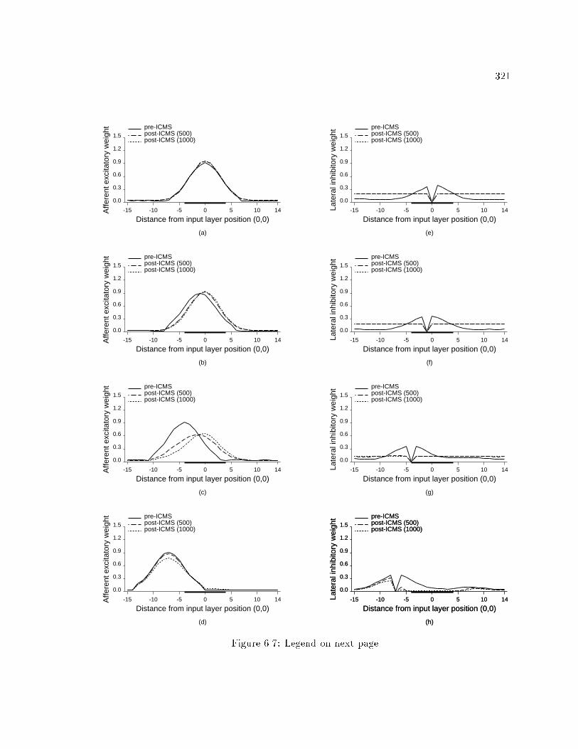
321-15 -10 -5 0 5 10 14

0.0

0.3

0.6

0.9

1.2

1.5

Affe

rent

exc

itato

ry w

eigh

t

Distance from input layer position (0,0)

pre-ICMSpost-ICMS (500)post-ICMS (1000)

(a)

-15 -10 -5 0 5 10 14

0.0

0.3

0.6

0.9

1.2

1.5

Affe

rent

exc

itato

ry w

eigh

t

Distance from input layer position (0,0)

pre-ICMSpost-ICMS (500)post-ICMS (1000)

(b)

-15 -10 -5 0 5 10 14

0.0

0.3

0.6

0.9

1.2

1.5

Affe

rent

exc

itato

ry w

eigh

t

Distance from input layer position (0,0)

pre-ICMSpost-ICMS (500)post-ICMS (1000)

(c)

-15 -10 -5 0 5 10 14

0.0

0.3

0.6

0.9

1.2

1.5

Affe

rent

exc

itato

ry w

eigh

t

Distance from input layer position (0,0)

pre-ICMSpost-ICMS (500)post-ICMS (1000)

(d)

-15 -10 -5 0 5 10 14

0.0

0.3

0.6

0.9

1.2

1.5

Late

ral i

nhib

itory

wei

ght

Distance from input layer position (0,0)

pre-ICMSpost-ICMS (500)post-ICMS (1000)

(e)

-15 -10 -5 0 5 10 14

0.0

0.3

0.6

0.9

1.2

1.5

Late

ral i

nhib

itory

wei

ght

Distance from input layer position (0,0)

pre-ICMSpost-ICMS (500)post-ICMS (1000)

(f)

-15 -10 -5 0 5 10 14

0.0

0.3

0.6

0.9

1.2

1.5

Late

ral i

nhib

itory

wei

ght

Distance from input layer position (0,0)

pre-ICMSpost-ICMS (500)post-ICMS (1000)

(g)

-15 -10 -5 0 5 10 14

0.0

0.3

0.6

0.9

1.2

1.5

Late

ral i

nhib

itory

wei

ght

Distance from input layer position (0,0)

pre-ICMSpost-ICMS (500)post-ICMS (1000)

(h)

-15 -10 -5 0 5 10 14

0.0

0.3

0.6

0.9

1.2

1.5

Late

ral i

nhib

itory

wei

ght

Distance from input layer position (0,0)

pre-ICMSpost-ICMS (500)post-ICMS (1000)

(h)Figure 6.7: Legend on next page.

322Figure 6.7: Pre- and post-ICMS a�erent excitatory and lateral inhibitorysynaptic weights.Figure on previous page. The �gure shows weights of a�erent excitatory pathways (leftcolumn) and lateral inhibitory pathways (right column) to di�erent model cortical neurons{ neuron (0; 0) in (a) and (e), neuron (0;�1) in (b) and (f), neuron (0;�4) in (c) and (g),and neuron (0;�7) in (d) and (h) { before ICMS, after 500 ICMS presentations, and after1000 ICMS presentations. In the EXIN network model, cortical neurons did not inhibitthemselves; i.e., the lateral inhibitory pathway from a neuron to itself was zero. Thus, thedistribution of the weights of lateral inhibitory pathways to a neuron has a dip. The thickline segment on the abscissa represents the neurons that were active during the initial stageof ICMS.so that the synaptic strength of the a�erents to the ICMS-site neuron remained almostunchanged (Figure 6.7). In Section 6.3.2 the e�ects of varying the presynaptic excitationto a�erent excitatory pathways are presented.In the model, the RFs of the model cortical neurons were topographically arranged,and all the neurons had almost identical RF sizes. In the cortex, however, the RF positionsare not strictly topographically arranged at a �ner level of detail, and RF sizes showlarge variations even among neighboring cortical neurons (Favorov & Kelly, 1996; Hubel &Wiesel, 1962; Recanzone et al., 1992b). In the model, if the neuron close to the ICMS sitehad a RF larger than the pre-ICMS ICMS-site RF size, it will receive stronger presynapticexcitation from a�erents selective to positions close to the ICMS-site RF center than froma�erents selective to positions far from the ICMS-site RF center. In this case, the RF sizeof the neuron will decrease to become almost identical to the pre-ICMS ICMS-site RF. If aneuron close to the ICMS site had a RF smaller than the pre-ICMS ICMS-site RF size, it willform strong synapses with a�erents selective to positions close to the ICMS-site RF center,and its RF size could increase because the lateral inhibition between the neurons close to theICMS site is weakened. In Section 6.3.3, ICMS is simulated in a network with RF scatter.Changes in RF sizeFigure 6.8a shows the RF size before and after ICMS as a function of the positionof the initial RF center. It is clear from the �gure that after ICMS1. the ICMS-site RF size increased by a very small amount;

323-15 -10 -5 0 5 10 14

0 0

10 10

20 20

30 30

40 40

50 50

RF

siz

e (a

rea)

Distance from ICMS site

pre-ICMSpost-ICMS

(a)

Pre-ICMSPost-ICMS

(b)

Mea

n R

F s

ize

(are

a)

Figure 6.8: Changes in RF size.(a) The �gure shows the RF area of neurons in a cross-section of model cortical layer passingthrough the ICMS site before and after ICMS. The thick line segment on the abscissarepresents the neurons active during the initial phase of ICMS. (b) The �gure shows themean RF area of model neurons before (white bar) and after (black bar) ICMS. The verticalline on the bars represent the standard deviation.2. the RF size of neurons closest to the ICMS site underwent very little change;3. the RF size of the neurons 2{4 units of distance away from the ICMS site showed adecrease in their RF size. These neurons were active during ICMS; and4. neurons 6{10 units of distance away from the ICMS site showed an increase in theirRF size. These neurons were inactive during ICMS.Thus, in the model, changes in RF size varied systematically with distance from theICMS site.Recanzone et al. (1992b) reported that after ICMS the mean RF size showed aslight increase. Figure 6.8b shows the pre- and post-ICMS mean RF sizes of the modelneurons.

324Changes in neuronal responsivenessFigure 6.9a shows the RF pro�le of the ICMS-site neuron, and Figure 6.9b showsthe maximal responsiveness of a one-dimensional cross-section of model cortical neuronsthrough the ICMS site, before and after ICMS. In the simulation, responsiveness of theneuron at the ICMS site showed very little change. This is consistent with results ofRecanzone et al. (1992b). In addition, maximal responsiveness of distal neurons increased.The distal neurons were inactive for most of the ICMS duration and therefore, the lateralinhibitory pathways to these neurons weakened (especially the strongly excited lateralinhibitory pathways from neurons close to the ICMS site), and the a�erent excitatorypathways to these neurons changed very little (e.g., neuron (0;�7) in Figure 6.7). Incontrast, maximal responsiveness of neurons surrounding the ICMS site decreased. Becausethe strength of excitation to the presynaptic a�erent excitatory terminals decreases asdistance from the ICMS site increases, neurons close to the ICMS site, which were activeduring ICMS, have weaker a�erent excitatory pathways after ICMS (e.g., neuron (0;�4) inFigure 6.7).Changes in RF positionIn the ICMS experiment, the RF of neurons close to the ICMS site shifted afterICMS toward the ICMS-site RF. However at cortical sites away from the ICMS site, someRFs shifted toward the ICMS-site RF and others shifted away from the ICMS-site RF atrandom (Recanzone et al., 1992b).In the model with topographically arranged RFs, the RF of most neurons shiftedtoward the ICMS-site RF (Figure 6.10). Small RF shifts away from the ICMS-site RF inthe RF of model neurons were seen in some neurons far from the ICMS site (Figure 6.30).Spatial distribution of the a�ected cortical regionIn the ICMS experiment, the cortical region a�ected by ICMS extendedasymmetrically around the ICMS site for several hundred microns. In addition, therewere sharp discontinuities at some locations between a region in which the RF of neurons

325-15 -10 -5 0 5 10 14

0

1

2

3

4

5IC

MS

-site

neu

ron

activ

ity

Distance from ICMS-site RF center

pre-ICMSpost-ICMS

(a)

-15 -10 -5 0 5 10 140

1

2

3

Max

imum

res

pons

e

Distance from ICMS site

pre-ICMSpost-ICMS

(b)Figure 6.9: Changes in neuronal responsiveness after ICMS.(a) One-dimensional RF pro�le of ICMS-site neuron. The RF pro�le was obtained byadding the neuron's response to input at positions along the y axis. (b) The maximalresponsiveness of neurons in a cross-section of the model cortical layer passing through theICMS site, neurons (0;�15){(0; 14), before and after ICMS. The thick line segment on theabscissa represents the neurons active during the initial stage of ICMS.

326-15 -10 -5 0 5 10 14

-5-4-3-2-1012345

RF

shi

ftou

twar

din

war

d

Distance from ICMS site

post-ICMS

Figure 6.10: RF shift after ICMS.The �gure shows the RF shift of neurons in a cross-section of the model cortical layer passingthrough the ICMS site after ICMS, neurons (0;�15){(0; 14). The thick line segment on theabscissa represents the neurons active during the initial phase of ICMS.overlapped with the pre-ICMS ICMS-site RF and an adjacent region in which the RF ofneurons did not overlap with the pre-ICMS ICMS-site RF (Recanzone et al., 1992b).A lack of systematic variation in the amount of overlap of the RF of neuronssurrounding the ICMS site and the ICMS-site RF may have occurred because thepre- and post-stimulation recordings were not necessarily from exactly the same neurons(Recanzone et al., 1992b). However, the neurons recorded at the same site before andafter ICMS were within 10{20 microns from each other (Recanzone et al., 1992b). Theobserved asymmetries in the distribution of RF changes over the cortical space may bedue to variations in the anatomical spread of arborizations of the thalamocortical a�erentsand/or the cortical axons and dendrites (Recanzone et al., 1992b).Figure 6.11 shows the amount of RF shift and the amount of overlap of theRF of model cortical neurons with the pre-ICMS ICMS-site RF after ICMS. In thesimulation, RF changes extended symmetrically over a large distance, and there wereno sharp discontinuities between regions containing neurons whose RF overlaps with the

327pre-ICMS ICMS-site RF and adjacent regions with neurons whose RF does not overlap withthe pre-ICMS ICMS-site RF.In the simulation, all model cortical neurons had similar a�erent and lateralconnectivity pro�les. In addition, the lateral inhibitory pathways were almost symmetrical.The uniformity in the connectivity patterns of the neurons is responsible for the systematicRF changes observed in this simulation. A more random connectivity pattern across modelcortical neurons results in less systematic RF changes during ICMS (Section 6.3.3).Temporal e�ects of ICMSThe cortical representation of the ICMS-site RF continues to increase withprogressively longer stimulation duration, and the e�ects of ICMS persist after cessationof ICMS (Recanzone et al., 1992b). In the simulation, additional conditioning led to anincrease in the overlap of the RF of model cortical neurons with the ICMS-site RF atfarther distances (Figures 6.12 and 6.14). In the absence of any stimulation, the e�ects ofICMS persisted in the model: synaptic plasticity in the model requires neuronal activation(Equations 6.4 and 6.6).In the simulation, the lateral inhibitory synaptic plasticity rate was faster thanthe a�erent excitatory synaptic plasticity rate (Appendix D, Section D.4.1). Thus, duringthe early stages of ICMS, RF changes were mainly caused by changes in the lateralinhibitory weights, and during the later stages, RF changes were mainly caused by thea�erent excitatory synaptic plasticity. At an early stage (after 250 ICMS steps), therewas a large increase in the number of neurons whose RF has 0-25% overlap with thepre-ICMS ICMS-site RF (Figure 6.12a). Since the ICMS causes model cortical neuronsto be weakly active, the faster lateral inhibitory synaptic plasticity caused weakening oflateral inhibitory pathways to neurons close to the ICMS site, thereby resulting in a smallincrease in neuronal responsiveness in the neurons close to the ICMS site (Figure 6.13).As ICMS proceeded (after 1000 ICMS steps), the a�erent excitatory synapticplasticity strengthened the a�erent pathways from the the pre-ICMS ICMS-site RF tothe active neurons near the ICMS site, thereby increasing the amount of overlap(Figure 6.12a). As more and more model cortical neurons became responsive to the

328ICMS site>75-100%>50-75%>25-50%>0-25%0%

Figure 6.11: Spatial distribution of changes in model cortical RF topography.The positions of the centroids of the RF of model cortical neurons before ICMS are presentedby the position of the center of the symbols. The lines code the shift of the centroid ofthe RF of the model cortical neurons after ICMS. The length of the lines represent theamount of shift, and the orientation of the lines represent the direction of shift. Thesymbols code the amount by which the RF of the model cortical neurons overlap with thepre-ICMS ICMS-site RF.

329

-15 -10 -5 0 5 10 1401020304050607080

RF

siz

e (a

rea)

Distance from ICMS site

Pre-ICMSAfter 250 iterationsAfter 500 iterationsAfter 1000 iterations

(b)

>0-25 >25-50 >50-75 >75-1000

50

100

150

200

250N

umbe

r of

neu

rons

Percent RF overlap with ICMS-site RF

Pre-ICMSAfter 250 iterationsAfter 500 iterationsAfter 1000 iterations

Far from ICMS site Close to ICMS site Adjacent to ICMS site(a)

-15 -10 -5 0 5 10 14-5-4-3-2-1012345

RF

shi

ftou

twar

din

war

d

Distance from ICMS site

After 250 iterationsAfter 500 iterationsAfter 1000 iterations

(c)Figure 6.12: Legend on next page.

330Figure 6.12: Temporal changes in RF topography and RF size during ICMS.Figure on previous page. (a) The number of model cortical neurons whose RF overlaps thepre-ICMS ICMS-site RF before and after ICMS. (b) RF area of neurons in a cross-sectionof the model cortical layer passing through the ICMS site, neurons (0;�15){(0; 14), beforeand after ICMS. (c) RF shift of neurons in a cross-section of the model cortical layer passingthrough the ICMS site after ICMS, neurons (0;�15){(0; 14). The line segment parallel tothe abscissa represents the neurons that were active during the initial stage of ICMS.-15 -10 -5 0 5 10 14

012345678

ICM

S-s

ite n

euro

n ac

tivity

Distance from ICMS-site RF center

Pre-ICMSAfter 250 iterationsAfter 500 iterationsAfter 1000 iterations

(a)

-15 -10 -5 0 5 10 140

1

2

3

Max

imum

res

pons

e

Distance from ICMS site

Pre-ICMSAfter 250 iterationsAfter 500 iterationsAfter 1000 iterations

(b)Figure 6.13: Temporal e�ects of ICMS on responsiveness.(a) One-dimensional RF pro�le of ICMS-site neuron. (b) The maximal responsivenessof neurons in a cross-section of the model cortical layer passing through the ICMS site,neurons (0;�15){(0; 14), at di�erent stages of ICMS. See Figure 6.9 for conventions.

331ICMS site>75-100%>50-75%>25-50%>0-25%0%

Figure 6.14: RF changes with additional ICMS.Changes in RF topography of model cortical neurons after 1000 steps of ICMS. SeeFigure 6.11 for conventions.

332same locations, their responsiveness to test stimuli decreased (Figure 6.13b). Thea�erent excitatory pathway weights to the ICMS-site neuron remained almost unchanged(Figure 6.7), and neurons surrounding the ICMS site strengthened synapses with a�erentexcitatory pathways from the the pre-ICMS ICMS-site RF (e.g., neurons (0,-1) and (0,-4)in Figure 6.7), and these neurons therefore had overlapping RFs. Because some neurons,e.g., neuron (0;�4) in Figure 6.7, weakened a�erent pathways from which they had thestrongest synapses, neurons close to the ICMS site became responsive to positions fartherfrom the pre-ICMS ICMS-site RF. Thus, the RF of neurons close to the ICMS site expanded(Figures 6.12b and 6.13a). Furthermore, as the amount of overlap of the RF of neuronsclose to the ICMS site with the pre-ICMS ICMS-site RF increased, the responsiveness ofneurons close to the ICMS site decreased (Figure 6.13b).The amount of shift in the RF of model cortical neurons toward thepre-ICMS ICMS-site RF increased with the number of ICMS time steps (Figure 6.12c).6.3.2 The e�ects of model ICMS parametersThis section illustrates the role of some of the parameters in the model, especiallythe speci�c e�ects of the a�erent excitatory synaptic plasticity, the lateral inhibitorysynaptic plasticity, and the distribution of presynaptic excitation to the a�erent excitatoryand lateral inhibitory pathways.Role of a�erent excitatory synaptic plasticityTo determine the e�ects of synaptic plasticity in a�erent excitatory pathways,ICMS was performed with the lateral inhibitory synaptic plasticity disabled. Withonly a�erent excitatory synaptic plasticity, active neurons strengthened their synapseswith strongly active a�erents and weaken their synapses with weakly active a�erents.Thus, the RF of these neurons shifted toward the ICMS-site RF (Figure 6.16c), andthere was an increase in number of neurons responsive to the pre-ICMS ICMS-site RF(Figures 6.16a and 6.17).In the absence of lateral inhibitory synaptic plasticity, as more active neuronsstrengthened synapses with a�erents selective to the ICMS-site RF, the ICMS-site neuron

333-15 -10 -5 0 5 10 14

0.0

0.3

0.6

0.9

1.2

1.5

Affe

rent

exc

itato

ry w

eigh

t

Distance from input layer position (0,0)

pre-ICMSpost-ICMS

(a)

-15 -10 -5 0 5 10 14

0.0

0.3

0.6

0.9

1.2

1.5

Affe

rent

exc

itato

ry w

eigh

t

Distance from input layer position (0,0)

pre-ICMSpost-ICMS

(b)

-15 -10 -5 0 5 10 14

0.0

0.3

0.6

0.9

1.2

1.5

Affe

rent

exc

itato

ry w

eigh

t

Distance from input layer position (0,0)

pre-ICMSpost-ICMS

(c)

-15 -10 -5 0 5 10 14

0.0

0.3

0.6

0.9

1.2

1.5

Affe

rent

exc

itato

ry w

eigh

t

Distance from input layer position (0,0)

pre-ICMSpost-ICMS

(d)

-15 -10 -5 0 5 10 14

0.0

0.3

0.6

0.9

1.2

1.5

Late

ral i

nhib

itory

wei

ght

Distance from input layer position (0,0)

pre-ICMSpost-ICMS

(e)

-15 -10 -5 0 5 10 14

0.0

0.3

0.6

0.9

1.2

1.5

Late

ral i

nhib

itory

wei

ght

Distance from input layer position (0,0)

pre-ICMSpost-ICMS

(f)

-15 -10 -5 0 5 10 14

0.0

0.3

0.6

0.9

1.2

1.5

Late

ral i

nhib

itory

wei

ght

Distance from input layer position (0,0)

pre-ICMSpost-ICMS

(g)

-15 -10 -5 0 5 10 14

0.0

0.3

0.6

0.9

1.2

1.5

Late

ral i

nhib

itory

wei

ght

Distance from input layer position (0,0)

pre-ICMSpost-ICMS

(h)Figure 6.15: Legend on next page.

334Figure 6.15: Changes pathway weights in ICMS simulations with a�erentexcitatory or lateral inhibitory synaptic plasticity disabled.Figure on previous page. Weights of a�erent excitatory pathways in the ICMS simulationwith lateral inhibitory synaptic plasticity disabled (left column), and weights of lateralinhibitory pathways in the ICMS simulation with a�erent excitatory synaptic plasticitydisabled (right column) to di�erent model cortical neurons are shown before ICMS andafter 500 ICMS presentations. (a,e) neuron (0; 0), (b,f) neuron (0;�1), (c,g) neuron (0;�4),and (d,h) neuron (0;�7). See Figure 6.7 for conventions.received more inhibition when the ICMS-site RF was stimulated. This led to a decreasein responsiveness of the ICMS-site neuron and neurons close to the stimulation site(Figure 6.18b). Because some neurons, e.g., neuron (0;�4) in Figure 6.15, weakened a�erentpathways from which they had the strongest synapses, neurons close to the ICMS sitebecame responsive to positions farther from the pre-ICMS ICMS-site RF. Thus, the RF ofneurons close to the ICMS site expanded (Figures 6.16b and 6.18a).Role of lateral inhibitory synaptic plasticityWith only lateral inhibitory synaptic plasticity, model ICMS resulted in weakeningof lateral inhibitory pathways to neurons close to the ICMS site, which were weakly active(Figure 6.15). This led to an increase in responsiveness (Figure 6.18b) and RF size ofmodel cortical neurons close to the ICMS site (Figures 6.16b and 6.18a). Because lateralinhibitory pathways from neurons close to the ICMS site to inactive/weakly active neuronsweakened more than lateral inhibitory pathways from neurons far from the ICMS site toinactive/weakly active neurons (Figure 6.15; see Section 6.4.1), the RF of neurons far fromthe ICMS site showed a small shift toward the ICMS-site RF (Figure 6.16c).Comparison of the e�ects of a�erent excitatory and lateral inhibitory synapticplasticityThe a�erent excitatory synaptic plasticity and the lateral inhibitory synapticplasticity produce complementary e�ects during ICMS. With both plasticity rules, theincrease in the number of neurons inhibiting the ICMS-site neuron when the ICMS-site RFis stimulated caused by the a�erent excitatory synaptic plasticity is balanced by the decrease

335

-15 -10 -5 0 5 10 1401020304050607080

RF

siz

e (a

rea)

Distance from ICMS site

Pre-ICMSBoth excitatory and inhibitory synaptic plasticityOnly excitatory synaptic plasticityOnly inhibitory synaptic plasticity

(b)

>0-25 >25-50 >50-75 >75-1000

50

100

150

200

250N

umbe

r of

neu

rons

Percent RF overlap with ICMS-site RF

Pre-ICMSBoth excitatory and inhibitory synaptic plasticityOnly excitatory synaptic plasticityOnly inhibitory synaptic plasticity

Far from ICMS site Close to ICMS site Adjacent to ICMS site(a)

-15 -10 -5 0 5 10 14-5-4-3-2-1012345

RF

shi

ftou

twar

din

war

d

Distance from ICMS site

Both excitatory and inhibitory synaptic plasticityOnly excitatory synaptic plasticityOnly inhibitory synaptic plasticity

(c)Figure 6.16: Role of a�erent excitatory and lateral inhibitory plasticity inproducing RF changes.In these simulations either the a�erent excitatory or the lateral inhibitory synaptic plasticityrule was disabled during ICMS. See Figure 6.12 for conventions.

336ICMS site>75-100%>50-75%>25-50%>0-25%0%

Figure 6.17: Changes in model cortical RF topography with only a�erentexcitatory plasticity.Only a�erent excitatory plasticity was enabled during model ICMS. See Figure 6.11 forconventions.

337-15 -10 -5 0 5 10 14

012345678

ICM

S-s

ite n

euro

n ac

tivity

Distance from ICMS-site RF center

Pre-ICMSBoth excitatory and inhibitory synaptic plasticityOnly excitatory synaptic plasticityOnly inhibitory synaptic plasticity

(a)

-15 -10 -5 0 5 10 140

1

2

3

Max

imum

res

pons

e

Distance from ICMS site

Pre-ICMSBoth excitatory and inhibitory synaptic plasticityOnly excitatory synaptic plasticityOnly inhibitory synaptic plasticity

(b)Figure 6.18: E�ect of a�erent excitatory plasticity and lateral inhibitory plasticityon responsiveness.See Figure 6.9 for conventions.

338in the strength of the lateral inhibitory pathways to the ICMS-site neuron. Furthermore,� a�erent excitatory synaptic plasticity increases the number of neurons whose RFshave more than 75% overlap with the ICMS-site RF, and these neurons are close tothe ICMS site (Figures 6.16b and 6.17), whereas lateral inhibitory synaptic plasticitymainly increases the number of neurons whose RFs have > 0{25% overlap with theICMS-site RF, and these neurons are far from the ICMS site (Figures 6.16a and 6.19);� a�erent excitatory synaptic plasticity alone produces RF expansion in neurons close tothe ICMS site and RF contraction in surrounding neurons, whereas lateral inhibitorysynaptic plasticity alone produces RF contraction in neurons close to the ICMS siteand RF expansion in surrounding neurons (Figures 6.16b and 6.18a);� a�erent excitatory synaptic plasticity alone produces large RF shifts toward theICMS-site RF in neurons close to the ICMS site, whereas lateral inhibitory synapticplasticity alone produces comparatively larger RF shifts toward the ICMS-site RF inneurons far from the ICMS site (Figure 6.16c); and� a�erent excitatory synaptic plasticity reduces responsiveness of neurons close to theICMS site; lateral inhibitory synaptic plasticity increases responsiveness of neuronsclose to the ICMS site (Figure 6.18b).E�ects of distribution of presynaptic stimulation of a�erent excitatory pathwaysIn the simulation in Section 6.3.1, a decrease in responsiveness of theICMS-site neuron caused by a�erent excitatory synaptic plasticity was balanced by thee�ects of lateral inhibitory synaptic plasticity. Another possibility for balancing for thedecrease in responsiveness of the ICMS-site neuron is to increase the strength of the a�erentexcitatory synapses. According to the EXIN a�erent excitatory synaptic plasticity rule, thea�erent excitatory synaptic strength equilibrates at a value proportional to the presynapticactivation. Thus, increasing the strength of presynaptic activation strengthens the a�erentpathways to the ICMS-site neuron.

339ICMS site>75-100%>50-75%>25-50%>0-25%0%

Figure 6.19: Changes in model cortical RF topography with only lateralinhibitory plasticity.A�erent excitatory synaptic plasticity was disabled during model ICMS. See Figure 6.11for conventions.

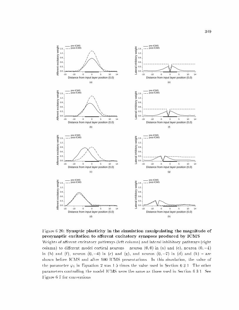
340-15 -10 -5 0 5 10 14

0.0

0.3

0.6

0.9

1.2

1.5

Affe

rent

exc

itato

ry w

eigh

t

Distance from input layer position (0,0)

pre-ICMSpost-ICMS

(a)

-15 -10 -5 0 5 10 14

0.0

0.3

0.6

0.9

1.2

1.5

Affe

rent

exc

itato

ry w

eigh

t

Distance from input layer position (0,0)

pre-ICMSpost-ICMS

(b)

-15 -10 -5 0 5 10 14

0.0

0.3

0.6

0.9

1.2

1.5

Affe

rent

exc

itato

ry w

eigh

t

Distance from input layer position (0,0)

pre-ICMSpost-ICMS

(c)

-15 -10 -5 0 5 10 14

0.0

0.3

0.6

0.9

1.2

1.5

Affe

rent

exc

itato

ry w

eigh

t

Distance from input layer position (0,0)

pre-ICMSpost-ICMS

(d)

-15 -10 -5 0 5 10 14

0.0

0.3

0.6

0.9

1.2

1.5

Late

ral i

nhib

itory

wei

ght

Distance from input layer position (0,0)

pre-ICMSpost-ICMS

(e)

-15 -10 -5 0 5 10 14

0.0

0.3

0.6

0.9

1.2

1.5

Late

ral i

nhib

itory

wei

ght

Distance from input layer position (0,0)

pre-ICMSpost-ICMS

(f)

-15 -10 -5 0 5 10 14

0.0

0.3

0.6

0.9

1.2

1.5La

tera

l inh

ibito

ry w

eigh

t

Distance from input layer position (0,0)

pre-ICMSpost-ICMS

(g)

-15 -10 -5 0 5 10 14

0.0

0.3

0.6

0.9

1.2

1.5

Late

ral i

nhib

itory

wei

ght

Distance from input layer position (0,0)

pre-ICMSpost-ICMS

(h)Figure 6.20: Synaptic plasticity in the simulation manipulating the magnitude ofpresynaptic excitation to a�erent excitatory synapses produced by ICMS.Weights of a�erent excitatory pathways (left column) and lateral inhibitory pathways (rightcolumn) to di�erent model cortical neurons { neuron (0; 0) in (a) and (e), neuron (0;�1)in (b) and (f), neuron (0;�4) in (c) and (g), and neuron (0;�7) in (d) and (h) { areshown before ICMS and after 500 ICMS presentations. In this simulation, the value ofthe parameter '1 in Equation 2 was 1.5 times the value used in Section 6.3.1. The otherparameters controlling the model ICMS were the same as those used in Section 6.3.1. SeeFigure 6.7 for conventions.

341-15 -10 -5 0 5 10 14

0.0

0.3

0.6

0.9

1.2

1.5

Affe

rent

exc

itato

ry w

eigh

t

Distance from input layer position (0,0)

pre-ICMSpost-ICMS

(a)

-15 -10 -5 0 5 10 14

0.0

0.3

0.6

0.9

1.2

1.5

Affe

rent

exc

itato

ry w

eigh

t

Distance from input layer position (0,0)

pre-ICMSpost-ICMS

(b)

-15 -10 -5 0 5 10 14

0.0

0.3

0.6

0.9

1.2

1.5

Affe

rent

exc

itato

ry w

eigh

t

Distance from input layer position (0,0)

pre-ICMSpost-ICMS

(c)

-15 -10 -5 0 5 10 14

0.0

0.3

0.6

0.9

1.2

1.5

Affe

rent

exc

itato

ry w

eigh

t

Distance from input layer position (0,0)

pre-ICMSpost-ICMS

(d)

-15 -10 -5 0 5 10 14

0.0

0.3

0.6

0.9

1.2

1.5

Late

ral i

nhib

itory

wei

ght

Distance from input layer position (0,0)

pre-ICMSpost-ICMS

(e)

-15 -10 -5 0 5 10 14

0.0

0.3

0.6

0.9

1.2

1.5

Late

ral i

nhib

itory

wei

ght

Distance from input layer position (0,0)

pre-ICMSpost-ICMS

(f)

-15 -10 -5 0 5 10 14

0.0

0.3

0.6

0.9

1.2

1.5La

tera

l inh

ibito

ry w

eigh

t

Distance from input layer position (0,0)

pre-ICMSpost-ICMS

(g)

-15 -10 -5 0 5 10 14

0.0

0.3

0.6

0.9

1.2

1.5

Late

ral i

nhib

itory

wei

ght

Distance from input layer position (0,0)

pre-ICMSpost-ICMS

(h)Figure 6.21: Synaptic plasticity in the simulation manipulating the distributionof presynaptic excitation to a�erent excitatory synapses produced by ICMS.Weights of a�erent excitatory pathways (left column) and lateral inhibitory pathways (rightcolumn) to di�erent model cortical neurons { neuron (0; 0) in (a) and (e), neuron (0;�1)in (b) and (f), neuron (0;�4) in (c) and (g), and neuron (0;�7) in (d) and (h) { areshown before ICMS and after 500 ICMS presentations. In this simulation, the value of theparameter �2 in Equation 2 was twice the value used in Section 6.3.1. The other parameterscontrolling the model ICMS were the same as those used in Section 6.3.1. See Figure 6.7for conventions.

342

-15 -10 -5 0 5 10 140

1020304050607080

RF

siz

e (a

rea)

Distance from ICMS site

Pre-ICMSNormal presynaptic excitation to afferent excitatory pathwaysStronger excitation to afferent excitatory pathways (ϕ1 x 1.5)Stronger excitation to afferent excitatory pathways and no lateral inhibitory plasticity (ϕ1 x 1.5)

(b)

>0-25 >25-50 >50-75 >75-1000

50

100

150

200

250

Num

ber

of n

euro

ns

Percent RF overlap with ICMS-site RF

Pre-ICMSNormal presynaptic excitation to afferent excitatory pathwaysStronger excitation to afferent excitatory pathways (ϕ1 x 1.5)Stronger excitation to afferent excitatory pathways and no lateral inhibitory plasticity (ϕ1 x 1.5)

Far from ICMS site Close to ICMS site Adjacent to ICMS site(a)

-15 -10 -5 0 5 10 14-5-4-3-2-1012345

RF

shi

ftou

twar

din

war

d

Distance from ICMS site

Normal presynaptic excitation to afferent excitatory pathwaysStronger excitation to afferent excitatory pathways (ϕ1 x 1.5)Stronger excitation to afferent excitatory pathways and no lateral inhibitory plasticity (ϕ1 x 1.5)

(c)Figure 6.22: Legend on next page.

343Figure 6.22: E�ects of the strength of presynaptic excitation of a�erent excitatorypathways on model RF size and position.Figure on previous page. Some of the e�ects of varying presynaptic excitation strength ofthe a�erent excitatory pathways during ICMS are shown. The values of the parametersin Equation 2 are given in Figure 6.5. (a) The number of model cortical neurons withRF overlapping the pre-ICMS ICMS-site RF before and after ICMS. (b) RF area ofneurons (0;�15){(0; 14), before and after ICMS. (c) RF shift of neurons in a cross-sectionof the model cortex passing through the ICMS site after ICMS, neurons (0;�15){(0; 14).The line segments parallel to the abscissa represent the neurons that were active during theinitial ICMS step as the ICMS parameters were varied.When ICMS was simulated in the EXIN network with stronger stimulation ofthe a�erent excitatory pathways (i.e., '1 in Equation 6.2 was increased) and with thelateral inhibitory synaptic plasticity disabled, there was a large increase in the RF size ofneurons close to the ICMS site (Figures 6.22b and 6.23a), and the responsiveness of theICMS-site neuron was almost equal to the pre-ICMS ICMS-site neuronal responsiveness(Figure 6.23b). With a smaller value for '1, the responsiveness of the ICMS-site neuronin the EXIN network with the lateral inhibitory synaptic plasticity disabled was smaller(Figure 6.18b).When the ICMS was simulated with both a�erent excitatory and lateral inhibitorysynaptic plasticity and with a larger '1, the neuronal responsiveness of the ICMS-site neurondecreased (Figure 6.23b) but its RF size remained close to the pre-ICMS size (Figure 6.22b).Stronger stimulation of the a�erent excitatory pathways during ICMS caused neurons closeto the ICMS site to be more strongly activated (Figure 6.5), which led to strengthening oflateral inhibitory pathways to these neurons and to a decrease in neuronal responsiveness ofthese neurons. Since the presynaptic activation level of the a�erent excitatory pathways tothe ICMS-site neuron was larger, the a�erent excitatory synaptic plasticity rule caused thesepathways to strengthen (Figure 6.20). In this simulation, the e�ects of stronger a�erentexcitatory and lateral inhibitory pathways to the ICMS-site neuron combined to produceno change in the size of the ICMS-site RF after ICMS (Figures 6.22b and 6.23a). When'1 in Equation 6.2 was increased, the EXIN model produced an increase in the overlap ofthe RF of model cortical neurons with the pre-ICMS ICMS-site RF (Figure 6.22a) and inRF shifts toward the pre-ICMS ICMS-site RF (Figure 6.22c).

344-15 -10 -5 0 5 10 14

012345678

ICM

S-s

ite n

euro

n ac

tivity

Distance from ICMS-site RF center

Pre-ICMSNormal presynaptic excitation to afferent excitatory pathwaysStronger excitation to afferent excitatory pathways (ϕ1 x 1.5)Stronger excitation to afferent excitatory pathways and no lateral inhibitory plasticity (ϕ1 x 1.5)

(a)

-15 -10 -5 0 5 10 140

1

2

3

Max

imum

res

pons

e

Distance from ICMS site

Pre-ICMSNormal presynaptic excitation to afferent excitatory pathwaysStronger excitation to afferent excitatory pathways (ϕ1 x 1.5)Stronger excitation to afferent excitatory pathways and no lateral inhibitory plasticity (ϕ1 x 1.5)

(b)Figure 6.23: E�ects of excitation strength of the presynaptic a�erent excitatorypathways on model responsiveness.Some of the e�ects of varying presynaptic excitation strength of the a�erent excitatorypathways during ICMS are shown. The values of the parameters in Equation 2 are givenin Figure 6.5. (a) One-dimensional RF pro�le of ICMS-site neuron. The RF pro�le wasobtained by adding the neuron's response to input at positions along the y axis. (b) Themaximal responsiveness of neurons in a cross-section of model cortical layer passing throughthe ICMS site, neurons (0;�15){(0; 14), before and after ICMS. The line segments parallelto the abscissa represent the neurons that were active during the initial ICMS step as theICMS parameters were varied.

345

-15 -10 -5 0 5 10 1401020304050607080

RF

siz

e (a

rea)

Distance from ICMS site

Pre-ICMSNormal presynaptic excitation to afferent excitatory pathwaysBroader distribution of excitation to afferent excitatory pathways (σ2 x 2)Smaller fall-off rate of effect of ICMS on excitation to afferent excitatory pathways (σ3 x 2)Larger baseline excitation to afferent excitatory pathways (φ1 x 2)

(b)

>0-25 >25-50 >50-75 >75-1000

50

100

150

200

250N

umbe

r of

neu

rons

Percent RF overlap with ICMS-site RF

Pre-ICMSNormal presynaptic excitation to afferent excitatory pathwaysBroader distribution of excitation to afferent excitatory pathways (σ2 x 2)Smaller fall-off rate of effect of ICMS on excitation to afferent excitatory pathways (σ3 x 2)Larger baseline excitation to afferent excitatory pathways (φ1 x 2)

Far from ICMS site Close to ICMS site Adjacent to ICMS site(a)

-15 -10 -5 0 5 10 14-5-4-3-2-1012345

RF

shi

ftou

twar

din

war

d

Distance from ICMS site

Normal presynaptic excitation to afferent excitatory pathwaysBroader distribution of excitation to afferent excitatory pathways (σ2 x 2)Smaller fall-off rate of effect of ICMS on excitation to afferent excitatory pathways (σ3 x 2)Larger baseline excitation to afferent excitatory pathways (φ1 x 2)

(c)Figure 6.24: E�ects of presynaptic stimulation distribution to the a�erentexcitatory pathways on model RF properties.Some of the e�ects of varying the presynaptic stimulation distribution to the a�erentexcitatory pathways during ICMS are shown. The values of the parameters in Equation 2are given in Figure 6.5. See Figure 6.22 for conventions. In this �gure, the line segmentsparallel to the abscissa are of di�erent lengths because as the ICMS parameters were variedthe distribution of active model cortical neurons was di�erent (see Figure 6.5).

346-15 -10 -5 0 5 10 14

012345678

ICM

S-s

ite n

euro

n ac

tivity

Distance from ICMS-site RF center

Pre-ICMSNormal excitation to afferent excitatory pathwaysBroader distribution of excitation to afferent excitatory pathways (σ2 x 2)Smaller fall-off rate of effect of ICMS on excitation to afferent excitatory pathways (σ3 x 2)Larger baseline excitation to afferent excitatory pathways (φ1 x 2)

(a)

-15 -10 -5 0 5 10 140

1

2

3

Max

imum

res

pons

e

Distance from ICMS site

Pre-ICMSNormal excitation to afferent excitatory pathwaysBroader distribution of excitation to afferent excitatory pathways (σ2 x 2)Smaller fall-off rate of effect of ICMS on excitation to afferent excitatory pathways (σ3 x 2)Larger baseline excitation to afferent excitatory pathways (φ1 x 2)

(b)Figure 6.25: E�ects of presynaptic stimulation distribution to the a�erentexcitatory pathways on model responsiveness.Some of the e�ects of varying the presynaptic stimulation distribution to the a�erentexcitatory pathways during ICMS are shown. The values of the parameters in Equation 2are given in Figure 6.5. See Figure 6.23 for conventions. In this �gure, the line segmentsparallel to the abscissa are of di�erent lengths because as the ICMS parameters were variedthe distribution of active model cortical neurons was di�erent (see Figure 6.5).

347Figures 6.24 and 6.25 show the e�ects of varying other parameters in Equation 6.2(�1, �2, and �3). As these parameters are varied, the EXIN synaptic plasticity rulesproduce an increase in the number of neurons whose RF has more than 75% overlapwith the pre-ICMS ICMS-site RF (Figure 6.24a), a contraction of the RF of neuronsclose to the ICMS site, an expansion of the RF of neurons far from the ICMS siteexpands (Figure 6.24b), a shift in the RF of model cortical neurons towards thepre-ICMS ICMS-site RF (Figure 6.24c), a decrease in the responsiveness of neurons closeto the ICMS site, and an increase in the responsiveness of neurons far from the ICMS site(Figure 6.25b). This shows that the proposed model is quite robust in producing changes inRF properties following ICMS similar to those observed experimentally. However, as theseparameters are varied, the RF size of the ICMS-site neuron and the ICMS-site neuronalresponsiveness to test stimuli change (Figures 6.24b and 6.25b).The changes in ICMS-site neuronal responsiveness to test stimuli are correlatedwith the activation level of the ICMS-site neuron in the initial stage of ICMS. In general,as the activation level of the ICMS-site neuron in the initial stage of ICMS increases,the RF size of the ICMS-site neuron and the ICMS-site neuronal responsiveness to teststimuli after ICMS decrease (Figures 6.5, 6.24b, and 6.25ab). As the activation level of theICMS-site neuron in the initial stage of ICMS increases, the lateral inhibitory pathwaysto the ICMS-site neuron strengthen, according to the EXIN lateral inhibitory synapticplasticity rule, thereby reducing the ICMS-site neuron's RF size and responsiveness to thetest input.The relationship between the activation level of the ICMS-site neuron in the initialstage of ICMS and the various parameters in Equation 6.2 is as follows. As the baselinestimulation strength of the a�erent excitatory pathways (�1 in Equation 6.2) is increased,excitation to the ICMS-site neuron increases (Equation 6.9), and therefore the activationof the neuron increases (Figure 6.5). The activation of the ICMS-site neuron increases(Figure 6.5) as the distribution of the stimulation strength of the a�erent excitatorypathways to the model cortical neurons is broadened (i.e., �2 in Equation 6.2 is increased)because increasing �2 increases a�erent excitation to the ICMS-site neuron (Equation 6.9).The activation of neurons close to the ICMS site decreases (Figure 6.5) as the fall-o� rate

348of the strength of the ICMS to the a�erent excitatory pathways is reduced (i.e., �3 inEquation 6.2 is increased), because excitation to the ICMS-site neuron remains the samebut the excitation to neurons surrounding the ICMS site increases, which in turn increasesthe activation of the surrounding neurons. As the activation of the surrounding neuronsincreases they exert greater inhibition on the ICMS-site neuron, leading to a decrease inthe activation of the ICMS-site neuron.Figures 6.27 and 6.28 show the e�ects of varying the parameters in Equation 6.1.Increasing '0 in Equation 6.1 increases excitation to the ICMS-site neuron and increasesthe activation of the ICMS-site neuron in the initial stage of ICMS (Figure 6.26). Increasing�1 in Equation 6.1 increases excitation to neurons surrounding the ICMS-site neuronand decreases the activation level of the ICMS-site neuron in the initial stage ofICMS (Figure 6.26). ICMS with the larger '0 decreased the ICMS-site RF size(Figures 6.27b and 6.28a) and decreased ICMS-site neuronal responsiveness to teststimuli (Figure 6.28b). ICMS with the larger �1 increased ICMS-site RF size(Figures 6.27b and 6.28a) and increased ICMS-site neuronal responsiveness to test stimuli(Figure 6.28b). Changes in RF properties of other model cortical neurons were similar tothose presented in Section 6.3.1.E�ects of distribution of presynaptic stimulation of lateral inhibitory pathwaysFigures 6.30{6.33 show the e�ects of varying the parameters in Equation 6.3 (�2,'2, �4, and �5). As these parameters are increased, the EXIN synaptic plasticity rulesproduce an increase in the number of neurons whose RF has a large overlap with thepre-ICMS ICMS-site RF (Figures 6.30a and 6.32a), a contraction of the RF of neuronsclose to the ICMS site and an expansion of the RF of neurons far from the ICMS site(Figures 6.30b and 6.32b), a shift of the RF of model cortical neurons towards thepre-ICMS ICMS-site RF (Figures 6.30c and 6.32c), a decrease in responsiveness of neuronsclose to the ICMS site, and an increase in responsiveness of neurons far from the ICMS site(Figures 6.31b and 6.33b). Thus, the proposed model is quite robust in producing changes inRF properties following ICMS similar to those observed experimentally. However, as theseparameters are varied, the RF size of the ICMS-site neuron and the ICMS-site neuronal

349

-15 -10 -5 0 5 10 14

-0.300

-0.220

-0.140

-0.060

0.020

0.100

0.180

0.260

0.340

0.420

0.500

Neu

ron

activ

ity

Distance from ICMS-site neuron

Normal distribution of direct excitation to cortical neurons

-15 -10 -5 0 5 10 14

-0.300

-0.220

-0.140

-0.060

0.020

0.100

0.180

0.260

0.340

0.420

0.500

Neu

ron

activ

ity

Distance from ICMS-site neuron

Stronger direct excitation to cortical neurons (ϕ 0 x 2000)

-15 -10 -5 0 5 10 14

-0.300

-0.220

-0.140

-0.060

0.020

0.100

0.180

0.260

0.340

0.420

0.500

Neu

ron

activ

ity

Distance from ICMS-site neuron

Stronger and broader distribution of direct excitation to cortical neurons ( σ 1 x 10)

Figure 6.26: Changes in activation of model neurons caused by changes in thedistribution of direct excitation to the neurons.The activations of a cross-section of model cortical layer neurons through the ICMS site,neurons (0;�15){(0; 14), in the initial stage of ICMS, as parameter values in Equation 1are varied, are shown. The parameter values in Equations 2 and 3 were the same as thoseused in the simulations presented in Section 6.3.1 (see Appendix D, Section D.4.1). For thenormal distribution of direct excitation to model cortical neurons, the values of parametersin Equation 1 were the same as those used in Section 6.3.1. For stronger direct excitationto cortical neurons, the value of '0 in Section 6.3.1 was multiplied by 2000, and for broaderdistribution of direct excitation to cortical neurons, the value of �1 in Section 6.3.1 wasmultiplied by 10.

350

-15 -10 -5 0 5 10 1401020304050607080

RF

siz

e (a

rea)

Distance from ICMS site

Pre-ICMSNormal distribution of excitation to cortical neuronsStronger direct excitation to cortical neurons (ϕ0 x 2000)Stronger and broader distribution of direct excitation to cortical neurons (σ1 x 10)

(b)

>0-25 >25-50 >50-75 >75-1000

50

100

150

200

250N

umbe

r of

neu

rons

Percent RF overlap with ICMS-site RF

Pre-ICMSNormal distribution of excitation to cortical neuronsStronger direct excitation to cortical neurons (ϕ0 x 2000)Stronger and broader distribution of direct excitation to cortical neurons (σ1 x 10)

Far from ICMS site Close to ICMS site Adjacent to ICMS site(a)

-15 -10 -5 0 5 10 14-5-4-3-2-1012345

RF

shi

ftou

twar

din

war

d

Distance from ICMS site

Normal distribution of excitation to cortical neuronsStronger direct excitation to cortical neurons (ϕ0 x 2000)Stronger and broader distribution of direct excitation to cortical neurons (σ1 x 10)

(c)Figure 6.27: E�ects of distribution of direct stimulation to the model corticalneurons on RF properties.Some of the e�ects of varying the parameters controlling direct excitation to the modelcortical neurons during ICMS are shown. The values of the parameters in Equation 1 aregive in Figure 6.26. See Figure 6.22 for conventions.

351-15 -10 -5 0 5 10 14

012345678

ICM

S-s

ite n

euro

n ac

tivity

Distance from ICMS-site RF center

Pre-ICMSNormal distribution of excitation to cortical neuronsStronger direct excitation to cortical neurons (ϕ0 x 2000)Stronger and broader distribution of direct excitation to cortical neurons (σ1 x 10)

(a)

-15 -10 -5 0 5 10 140

1

2

3

Max

imum

res

pons

e

Distance from ICMS site

Pre-ICMSNormal distribution of excitation to cortical neuronsStronger direct excitation to cortical neurons (ϕ0 x 2000)Stronger and broader distribution of direct excitation to cortical neurons (σ1 x 10)

(b)Figure 6.28: E�ects of distribution of direct stimulation to the model corticalneurons on responsiveness.Some of the e�ects of varying the parameters controlling direct excitation to the modelcortical neurons during ICMS are shown. The values of the parameters in Equation 1 aregive in Figure 6.26. See Figure 6.23 for conventions.

352

-15 -10 -5 0 5 10 14

-0.300

-0.220

-0.140

-0.060

0.020

0.100

0.180

0.260

0.340

0.420

0.500

Neu

ron

activ

ity

Distance from ICMS-site neuron

Normal distribution of excitation to lateral inhibitory pathways

-15 -10 -5 0 5 10 14

-0.300

-0.220

-0.140

-0.060

0.020

0.100

0.180

0.260

0.340

0.420

0.500

Neu

ron

activ

ity

Distance from ICMS-site neuron

Stronger excitation to lateral inhibitory pathways (ϕ 2 x 2)

-15 -10 -5 0 5 10 14

-0.300

-0.220

-0.140

-0.060

0.020

0.100

0.180

0.260

0.340

0.420

0.500

Neu

ron

activ

ity

Distance from ICMS-site neuron

Broader distribution of excitation to lateral inhibitory pathways (σ 4 x 2)

-15 -10 -5 0 5 10 14

-0.300

-0.220

-0.140

-0.060

0.020

0.100

0.180

0.260

0.340

0.420

0.500

Neu

ron

activ

ity

Distance from ICMS-site neuron

Smaller fall-off rate of effect of ICMS on excitation to lateral inhibitory pathways (σ 5 x 2)

-15 -10 -5 0 5 10 14

-0.300

-0.220

-0.140

-0.060

0.020

0.100

0.180

0.260

0.340

0.420

0.500

Neu

ron

activ

ity

Distance from ICMS-site neuron

Larger baseline excitation to lateral inhibitory pathways (φ2 x 2)

Figure 6.29: Changes in activation of model neurons caused by changes in thedistribution of presynaptic excitation to lateral inhibitory pathways.The activation of a cross-section of model cortical layer neurons through the ICMS site,i.e., neurons (0;�15){(0; 14), in the initial stage of ICMS, as parameter values in Equation 3are varied, are shown. The parameter values in Equations 1 and 2 were the same as thoseused in the simulations presented in Section 6.3.1 (see Appendix D, Section D.4.1). Forthe normal distribution of excitation to lateral inhibitory pathways, the parameters inEquation 3 were assigned the values used in the ICMS simulation in Section 6.3.1. Forstronger excitation to the lateral inhibitory pathways, the value of '2 in Section 6.3.1 wasmultiplied by a factor of 2; for broader distribution of excitation to the lateral inhibitorypathways, the value of �4 used in Section 6.3.1 was multiplied 2; for a smaller fall-o� rateof the e�ect of ICMS on excitation to the lateral inhibitory pathways, the value of �5 inSection 6.3.1 was multiplied by 2; and for a larger baseline excitation to the lateral inhibitorypathways, the value of �2 used in Section 6.3.1 was multiplied by 2.

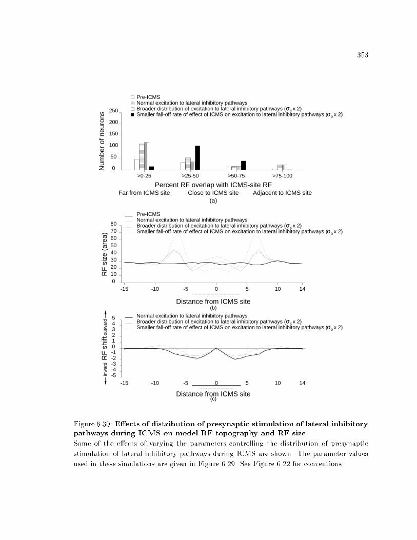
353

-15 -10 -5 0 5 10 140

1020304050607080

RF

siz

e (a

rea)

Distance from ICMS site

Pre-ICMSNormal excitation to lateral inhibitory pathwaysBroader distribution of excitation to lateral inhibitory pathways (σ4 x 2)Smaller fall-off rate of effect of ICMS on excitation to lateral inhibitory pathways (σ5 x 2)

(b)

>0-25 >25-50 >50-75 >75-1000

50

100

150

200

250

Num

ber

of n

euro

ns

Percent RF overlap with ICMS-site RF

Pre-ICMSNormal excitation to lateral inhibitory pathwaysBroader distribution of excitation to lateral inhibitory pathways (σ4 x 2)Smaller fall-off rate of effect of ICMS on excitation to lateral inhibitory pathways (σ5 x 2)

Far from ICMS site Close to ICMS site Adjacent to ICMS site(a)

-15 -10 -5 0 5 10 14-5-4-3-2-1012345

RF

shi

ftou

twar

din

war

d

Distance from ICMS site

Normal excitation to lateral inhibitory pathwaysBroader distribution of excitation to lateral inhibitory pathways (σ4 x 2)Smaller fall-off rate of effect of ICMS on excitation to lateral inhibitory pathways (σ5 x 2)

(c)Figure 6.30: E�ects of distribution of presynaptic stimulation of lateral inhibitorypathways during ICMS on model RF topography and RF size.Some of the e�ects of varying the parameters controlling the distribution of presynapticstimulation of lateral inhibitory pathways during ICMS are shown. The parameter valuesused in these simulations are given in Figure 6.29. See Figure 6.22 for conventions.

354-15 -10 -5 0 5 10 14

012345678

ICM

S-s

ite n

euro

n ac

tivity

Distance from ICMS-site RF center

Pre-ICMSNormal excitation to lateral inhibitory pathwaysBroader distribution of excitation to lateral inhibitory pathways (σ4 x 2)Smaller fall-off rate of effect of ICMS on excitation to lateral inhibitory pathways (σ5 x 2)

(a)

-15 -10 -5 0 5 10 140

1

2

3

Max

imum

res

pons

e

Distance from ICMS site

Pre-ICMSNormal excitation to lateral inhibitory pathwaysBroader distribution of excitation to lateral inhibitory pathways (σ4 x 2)Smaller fall-off rate of effect of ICMS on excitation to lateral inhibitory pathways (σ5 x 2)

(b)Figure 6.31: E�ects of distribution of presynaptic stimulation of lateral inhibitorypathways during ICMS on model responsiveness.The parameter values used in these simulations are given in Figure 6.29. See Figure 6.23for conventions.

355

-15 -10 -5 0 5 10 1401020304050607080

RF

siz

e (a

rea)

Distance from ICMS site

Pre-ICMSNormal excitation to lateral inhibitory pathwaysStronger excitation to lateral inhibitory pathways (ϕ2 x 2)Larger baseline excitation to lateral inhibitory pathways (φ2 x 2)

(b)

>0-25 >25-50 >50-75 >75-1000

50

100

150

200

250N

umbe

r of

neu

rons

Percent RF overlap with ICMS-site RF

Pre-ICMSNormal excitation to lateral inhibitory pathwaysStronger excitation to lateral inhibitory pathways (ϕ2 x 2)Larger baseline excitation to lateral inhibitory pathways (φ2 x 2)

Far from ICMS site Close to ICMS site Adjacent to ICMS site(a)

-15 -10 -5 0 5 10 14-5-4-3-2-1012345

RF

shi

ftou

twar

din

war

d

Distance from ICMS site

Normal excitation to lateral inhibitory pathwaysStronger excitation to lateral inhibitory pathways (ϕ2 x 2)Larger baseline excitation to lateral inhibitory pathways (φ2 x 2)

(c)Figure 6.32: E�ects of distribution of presynaptic stimulation of lateral inhibitorypathways during ICMS on model RF topography and RF size.The parameter values used in these simulations are given in Figure 6.29. See Figure 6.22for conventions.

356-15 -10 -5 0 5 10 14

012345678

ICM

S-s

ite n

euro

n ac

tivity

Distance from ICMS-site RF center

Pre-ICMSNormal excitation to lateral inhibitory pathwaysStronger excitation to lateral inhibitory pathways (ϕ2 x 2)Larger baseline excitation to lateral inhibitory pathways (φ2 x 2)

(a)

-15 -10 -5 0 5 10 140

1

2

3

Max

imum

res

pons

e

Distance from ICMS site

Pre-ICMSNormal excitation to lateral inhibitory pathwaysStronger excitation to lateral inhibitory pathways (ϕ2 x 2)Larger baseline excitation to lateral inhibitory pathways (φ2 x 2)

(b)Figure 6.33: E�ects of distribution of presynaptic stimulation of lateral inhibitorypathways during ICMS on model responsiveness.The parameter values used in these simulations are given in Figure 6.29. See Figure 6.23for conventions.

357responsiveness to test stimuli change (Figures 6.30b and 6.32b).Changes in the parameters controlling the strength and distribution of stimulationof the lateral inhibitory pathways directly a�ect the activation level of the model corticalneurons. As the activation of the ICMS-site neuron in the initial stage of ICMS increases, theRF size of the ICMS-site neuron and the ICMS-site neuronal responsiveness to test stimuliafter ICMS decrease (Figures 6.29, 6.30 { 6.33). As activation of the ICMS-site neuronin the initial stage of ICMS increases, the lateral inhibitory pathways to the ICMS-siteneuron strengthen according to the EXIN lateral inhibitory synaptic plasticity rule, therebyreducing the ICMS-site neuron's RF size and responsiveness to the test input.The relationship between the activation of the ICMS-site neuron in the initial stageof ICMS and the various parameters in Equation 6.3 are as follows. The activation of theICMS-site neuron decreases (Figure 6.29) as the distribution of the stimulation strengthof the lateral inhibitory pathways to the model cortical neurons is broadened (i.e., �4 inEquation 6.3 is increased) because increasing �4 increases the e�ect of lateral inhibition tothe ICMS-site neuron (Equation 6.10). The activation of neurons close to the ICMS siteincreases (Figure 6.29) as the fall-o� rate of the strength of the ICMS on inhibitory pathwaysis reduced (i.e., �5 in Equation 6.3 is increased), because inhibition to the ICMS-site neuroncaused by stimulation of the lateral inhibitory pathways remains constant but the inhibitionto neurons surrounding the ICMS site caused by stimulation of the lateral inhibitorypathways increases, thereby decreasing the activation of the surrounding neurons. As theactivation of the surrounding neurons decreases, they exert less inhibition on the ICMS-siteneuron, leading to an increase in the activation of the ICMS-site neuron. As the stimulationstrength of the lateral inhibitory pathways increases (i.e., '2 in Equation 6.3 is increased)or as the baseline stimulation strength of the lateral inhibitory pathways increases (i.e., �2in Equation 6.3 is increased), inhibition to the ICMS-site neuron increases (Equation 6.10),and therefore the activation of the ICMS-site neuron decreases (Figure 6.29).When �5 in Equation 6.3 was increased, the increased inhibition to neuronsfar from the ICMS site kept those neurons inactive during ICMS, and according to theEXIN lateral inhibitory synaptic plasticity rule the lateral inhibitory pathways to thoseinactive neurons weakened. The weakening of the lateral inhibitory pathways to the distant

358neurons, which were inactive during ICMS, made these neurons highly responsive to teststimuli (Figure 6.31b). Such high responsiveness of these neurons resulted in large inhibitionto the surrounding neurons farther away from the ICMS site, and their RF shifted awayfrom the pre-ICMS ICMS site RF (Figure 6.30c).6.3.3 The e�ects of RF scatter during ICMSIn the earlier simulations, the RFs of the model cortical neurons weretopographically arranged. In this simulation, ICMS was performed in a network with initialRF scatter and non-uniform RF sizes (Figure 6.34). The parameters used were the same asthose used in the simulation presented in Section 6.3.1. The procedure for producing thenetwork with RF scatter is described in Appendix D, Section D.2.With RF scatter in the initial RF topography, the model reproduced all thequalitative aspects of the e�ects of ICMS (Figures 6.35{6.37). In particular, the modelproduced sharp discontinuities at some positions where a region containing neurons whoseRFs overlap the ICMS-site RF abuts another in which the RFs of the neurons do not overlapthe ICMS-site RF (Figure 6.35).In this simulation, the RF size, position, and responsiveness of the ICMS-siteneuron changed (Figures 6.36{6.37). This happened because the most strongly activatedmodel thalamocortical a�erents during ICMS were not the thalamocortical a�erents thathad the strongest synapses with the ICMS-site neuron.6.3.4 The e�ects of peripheral stimulationThe e�ects of repetitive peripheral stimulation of a restricted skin region weremodeled using lateral inhibitory plasticity and varying peripheral stimulation strength (seeSection 6.4.1). The results of Jenkins et al. (1990) were modeled by assuming that strongperipheral stimulation was used (Figure 6.38a), producing strong activation in the corticalneurons (Figure 6.38b). The changes in RF topography reported by Recanzone et al. (1992b)were modeled by weak peripheral stimulation (Figure 6.38cd).Jenkins et al. (1990) simulated �ngers of monkeys using a rotating disk withwedge-shaped indentations. The monkeys were required to keep their �ngers in contact

359ICMS site>75-100%>50-75%>25-50%>0-25%0%

Figure 6.34: Initial model cortical RF topography in the scatter simulation.The �gure shows scatter in the model cortical RFs after a training phase. The center ofthe symbols in the legend represent the expected position of the center of the RF of modelcortical neurons based on topographically arranged RFs. The line segments represent theshift in the center of the RF of the model cortical neurons away from the expected RFcenter.

360ICMS site>75-100%>50-75%>25-50%>0-25%0%

Figure 6.35: Changes in RF topography after ICMS in a network with RF scatter.Model ICMS was applied in a network whose initial RFs were not topographically arranged.See Figure 6.11 for conventions.

361

-15 -10 -5 0 5 10 1401020304050607080

RF

siz

e (a

rea)

Distance from ICMS site

Pre-ICMSPost-ICMS

(b)

>0-25 >25-50 >50-75 >75-1000

50

100

150

200

250N

umbe

r of

neu

rons

Percent RF overlap with ICMS-site RF

Pre-ICMSPost-ICMS

Far from ICMS site Close to ICMS site Adjacent to ICMS site(a)

-15 -10 -5 0 5 10 14-5-4-3-2-1012345

RF

shi

ftou

twar

din

war

d

Distance from ICMS site

Post-ICMS

(c)Figure 6.36: Changes in RF properties in a model network with RF scatter.Model ICMS was applied in a network with RF scatter. The model ICMS parameterswere the same as those used in the simulation in Section 6.3.1. The ICMS was presented500 times. See Figure 6.12 for conventions.

362-15 -10 -5 0 5 10 14

012345678

ICM

S-s

ite n

euro

n ac

tivity

Distance from ICMS-site RF center

Pre-ICMSPost-ICMS

(a)

-15 -10 -5 0 5 10 140

1

2

3

Max

imum

res

pons

e

Distance from ICMS site

Pre-ICMSPost-ICMS

(b)Figure 6.37: Changes in responsiveness in a model network with RF scatter.The model ICMS parameters were the same as those used in the simulation in Section 6.3.1.See Figure 6.9 for conventions.

363with the rotating disk. Because of the grooves on the disk it was di�cult to maintaincontact with the disk. Initially, the monkeys pressed their �ngers to the disk very stronglycausing their hands to be dragged by the rotating disk. Gradually, they learned to controlthe contact pressure to maintain contact with the rotating disk. Thus, the rotating diskmay have stimulated a large skin region. Furthermore, mechanoreceptors are much morestrongly activated by moving surfaces than at stationary surfaces, and a larger proportionof cutaneous mechanoreceptors are activated by moving ridged surfaces than at stationarysurfaces (Jenkins et al., 1990). On the other hand, Recanzone et al. (1990acde) useda tactile probe with a 2 mm diameter and a rounded tip. The probe was vibratedsinusoidally at a �xed frequency. The stimulation was applied to a �xed skin regionand was applied with a constant small force of about 6{10 gram weight. The area ofthe tactile probe used by Recanzone et al. (1992acde) was smaller than the RF sizeof the somatosensory cortical neurons. Thus, the stimulation procedure employed byJenkins et al. (1990) could have strongly stimulated a large skin region than the procedureused by Recanzone et al. (1992acde).When the input was a strong local stimulation, model cortical neurons werestrongly activated (Figure 6.38b). During conditioning, the lateral inhibitory pathwaysbetween the strongly active neurons strengthened, and lateral inhibitory pathways fromactive neurons to inactive neurons weakened. This caused a decrease in the RF size ofthe neurons activated by the conditioning input and an increase in the number of neuronsresponsive to the conditioning input (Figures 6.40{6.42). These results are qualitativelysimilar to those reported by Jenkins et al. (1990).When the input was a weak local stimulation, model cortical neurons were weaklyactivated (Figure 6.38d). During conditioning, the lateral inhibitory pathways between theweakly active neurons weakened, and the lateral inhibitory pathways from active neuronsto inactive neurons also weakened. This caused an increase in the RF size of the neuronsactivated by the conditioning input and an increase in the number of neurons responsive tothe conditioning input (Figures 6.40{6.42). These results are qualitatively similar to thosereported by Recanzone et al. (1992b).

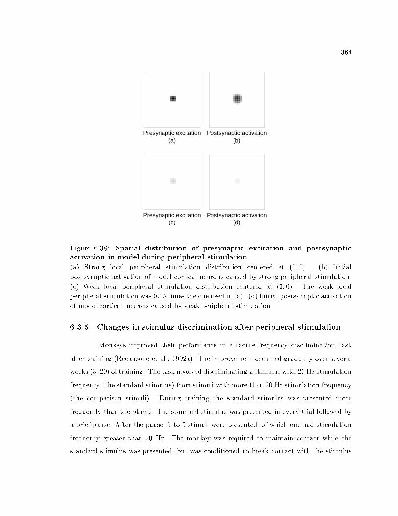
364Presynaptic excitation

(a)Postsynaptic activation

(b)

Presynaptic excitation(c)

Postsynaptic activation(d)Figure 6.38: Spatial distribution of presynaptic excitation and postsynapticactivation in model during peripheral stimulation.(a) Strong local peripheral stimulation distribution centered at (0; 0). (b) Initialpostsynaptic activation of model cortical neurons caused by strong peripheral stimulation.(c) Weak local peripheral stimulation distribution centered at (0; 0). The weak localperipheral stimulation was 0:15 times the one used in (a). (d) Initial postsynaptic activationof model cortical neurons caused by weak peripheral stimulation.6.3.5 Changes in stimulus discrimination after peripheral stimulationMonkeys improved their performance in a tactile frequency discrimination taskafter training (Recanzone et al., 1992a). The improvement occurred gradually over severalweeks (3{20) of training. The task involved discriminating a stimulus with 20 Hz stimulationfrequency (the standard stimulus) from stimuli with more than 20 Hz stimulation frequency(the comparison stimuli). During training the standard stimulus was presented morefrequently than the others. The standard stimulus was presented in every trial followed bya brief pause. After the pause, 1 to 5 stimuli were presented, of which one had stimulationfrequency greater than 20 Hz. The monkey was required to maintain contact while thestandard stimulus was presented, but was conditioned to break contact with the stimulus

365-15 -10 -5 0 5 10 14

-0.300

-0.220

-0.140

-0.060

0.020

0.100

0.180

0.260

0.340

0.420

0.500

Neu

ron

activ

ity

Distance from ICMS-site neuron

Strong peripheral input

-15 -10 -5 0 5 10 14

-0.300

-0.220

-0.140

-0.060

0.020

0.100

0.180

0.260

0.340

0.420

0.500

Neu

ron

activ

ity

Distance from ICMS-site neuron

Weak peripheral input

Figure 6.39: Changes in activation of model neurons caused by variations inperipheral stimulation strength.The activation of a cross-section of the model cortical layer neurons, neurons (0;�15){(0; 14), in the initial stage of peripheral conditioning, is shown as the strength of theperipheral stimulus is varied. Strong local peripheral stimulation was the Gaussian K(Appendix D, Section D.5) centered at (0; 0). Weak local peripheral stimulation was0:15�K.if its stimulation frequency was greater than 20 Hz. The probability of occurrence of thecomparison stimuli was small (� 0:388).In the simulations, tactile frequency selectivity was not incorporated. Therefore,instead of tactile frequency discrimination, the stimulus position discrimination of the modelwas analyzed. The frequency of tactile stimulation can be encoded by distribution of activityin input �bers innervating mechanoreceptors. Mechanoreceptors in the skin have di�erenttemporal properties. The rapidly adapting (RA) mechanoreceptors respond selectivelyto high-frequency tactile stimulation and the slowly adapting (SA) mechanoreceptorsconvey information about constant pressure applied to skin. Thus, the frequency oftactile stimulation at a particular location is encoded in the distribution of activity inthe �bers innervating the RA and SA receptors. Furthermore, the �bers from RA andSA mechanoreceptors terminate in adjacent positions in the somatosensory cortex. Thus,

366

-15 -10 -5 0 5 10 140

1020304050607080

RF

siz

e (a

rea)

Distance from cortical neuron (0,0)

Pre-peripheral conditioningStrong peripheral input (1000 presentations)Weak peripheral input (1000 presentations)Weak peripheral input (2000 presentations)

(b)

>0-25 >25-50 >50-75 >75-1000

50

100

150

200

250N

umbe

r of

neu

rons

Percent RF overlap with RF of cortical neuron (0,0)

Pre-peripheral conditioningStrong peripheral input (1000 presentations)Weak peripheral input (1000 presentations)Weak peripheral input (2000 presentations)

Far from neuron (0,0) Close to neuron (0,0) Adjacent to neuron (0,0)(a)

-15 -10 -5 0 5 10 14-5-4-3-2-1012345

RF

shi

ftou

twar

din

war

d

Distance from cortical neuron (0,0)

Strong peripheral input (1000 presentations)Weak peripheral input (1000 presentations)Weak peripheral input (2000 presentations)

(c)Figure 6.40: Legend on next page.

367Figure 6.40: Changes in model RF properties caused by peripheral stimulation.Figure on previous page. In this simulation, the peripheral stimulation was centered atLayer 1 position (0; 0). Before conditioning the conditioning stimuli evoked the highestactivation in Layer 2 neuron (0; 0). The stimulus used for measurement of RF propertieswas also used as the strong peripheral stimulus. The weak peripheral stimulus was 0.15 timesthe stimulus used for measurement of RF properties. See Figure 6.12 for conventions. Theline segments parallel to the abscissa represent the neurons that were active during theinitial stage of the two peripheral conditioning simulations.-15 -10 -5 0 5 10 14

012345678

RF

pro

file

of c

ortic

al n

euro

n (0

,0)

Distance from peripheral stimulation site

Pre-peripheral conditioningStrong peripheral input (1000 presentations)Weak peripheral input (1000 presentations)Weak peripheral input (2000 presentations)

(a)

-15 -10 -5 0 5 10 140

1

2

3

Max

imum

res

pons

e

Distance from cortical neuron (0,0)

Pre-peripheral conditioningStrong peripheral input (1000 presentations)Weak peripheral input (1000 presentations)Weak peripheral input (2000 presentations)

(b)Figure 6.41: Changes in model neuron responsiveness caused by peripheralstimulation.Simulation details are presented in Figure 6.40. See Figure 6.9 for conventions. The linesegments parallel to the abscissa represent the neurons that were active during the initialstage of the two peripheral conditioning simulations.

368-15 -10 -5 0 5 10 14

020406080

100120140160180200

Cor

tical

mag

nific

atio

n

Distance from peripheral stimulation site

Pre-peripheral conditioningStrong peripheral input (1000 presentations)Weak peripheral input (1000 presentations)Weak peripheral input (2000 presentations)

Figure 6.42: Changes in model cortical magni�cation caused by peripheralstimulation.See Figure 6.40 for simulation details. Cortical magni�cation was computed as the numberof neurons responsive to the test stimulus at each input location. The �gure shows thecortical magni�cation of a cross-section of the input layer through the peripheral stimulationsite, input positions from (0;�15) to (0; 14), before and after peripheral conditioning. Theline segments parallel to the abscissa represent the neurons that were active during theinitial stage of the two peripheral conditioning simulations.changes in the frequency of a tactile stimulation changes the input distribution to adjacentneurons in the somatosensory cortex. This is similar to varying the position of the input inthe model.In the simulations, a conditioning stimulus was presented at a single position inthe input layer. The peripheral stimulation used in the simulations is an abstraction of thestimulation procedure used in Recanzone et al. (1992a) because the conditioning stimulationwas presented at only one position. Peripheral comparison stimuli were presented at otherlocations during the discrimination test phase, during which synaptic plasticity in the modelwas disabled.Changes in position discrimination were modeled by lateral inhibitory synapticplasticity. Figure 6.43 shows that discrimination between the conditioned input position andother test positions close to the conditioning site increased after training. The parameters

369-15 -10 -5 0 5 10 14

-2

-1

0

1

2

Cha

nge

in d

iscr

imin

atio

n(s

hift

in p

erce

ived

pos

ition

)

Distance from peripheral stimulation site

Strong input (1000 presentations)Weak input (1000 presentations)Weak input (2000 presentations)

incr

ease

decr

easeFigure 6.43: Changes in position discrimination after peripheral stimulation.Each model cortical neuron was assumed to code a particular position which was the centroidof its RF. The centroid was computed by weighting each input position by the response ofthe cortical neuron to test stimulus at that position. The position of the test stimuluswas interpreted from cortical activation produced by input stimulation by determiningthe centroid of the distribution of cortical activity in the input space; the centroid wascomputed by weighting the preferred position of each model cortical neuron by its activationin response to the test stimulus. As the amount of overlap in the distributions of corticalactivation produced by inputs at di�erent positions decreases, i.e., distance between thecentroids of cortical activation distributions increases, the chances of making errors indistinguishing the two positions because of noise in the neuronal activations decrease.Thus, position discrimination increases. In the simulations, the change in discriminationwas computed as the di�erence between the \perceived" position of the test stimuli afterconditioning and the \perceived" position of the test stimuli before conditioning. Increase indiscrimination represents a shift in the \perceived" position away from the conditioning site;decrease represents a shift towards the conditioning site.

370used in these simulations were the same as those used in the previous section (Section 6.3.4).The increase in position discrimination was obtained after stimulating the standard inputposition with strong and weak stimuli. The position discrimination was determined usingthe stimulus that was used to map the RF of the model cortical neurons. In the model,increase in position discrimination occurred with increase or decrease in the RF size andresponsiveness of model cortical neurons initially responsive to conditioning stimulation atthe conditioning site (Figures 6.40 and 6.41).In the simulations, position discrimination between the conditioning site and inputpositions close to the conditioning site increases because model cortical neurons selectivefor positions surrounding the conditioning site become more responsive to positions close tothe conditioning site relative to the responsiveness of neurons which were highly responsiveto stimulation at the conditioning site. Therefore, test stimulation at positions close toconditioning site activates neurons whose initial RFs were farther from the conditioningsite more strongly relative to the neurons whose RFs were closer to the conditioning site.This causes the \perceived" test stimulus position to shift farther away from the actualtest stimulation site. Thus, even a small shift in the position of the test stimulus from theconditioning site causes a large di�erence in the \perceived" position of the test stimulus.In the simulations, input positions at which position discrimination increased weresurrounded by positions at which position discrimination decreased (Figure 6.43). Teststimulation at positions where position discrimination decreased caused model corticalneurons responding to the test stimulus and closer to the cortical neurons selective forthe conditioning site to be more active than the neurons responding to the test stimulusand farther from the neurons selective for the conditioning site. This occured becausethe EXIN lateral inhibitory synaptic plasticity rule caused a large weakening in lateralinhibitory pathways from the active neurons to weakly active/inactive neurons whose RFsoverlap with the RFs of the active neurons, i.e., neurons close to the neurons selectivefor the conditioning site. According to the EXIN lateral inhibitory synaptic plasticityrule, plasticity is enabled only when the presynaptic neuron is active, and the strengthof lateral inhibitory synaptic weights becomes proportional to the amount of overlap inthe RFs of neurons (Marshall, 1995a). Thus, during peripheral stimulation the lateral

371inhibitory pathways from the active neurons to weakly active/inactive neurons weaken,and maximal weakening occurs in lateral inhibitory pathways from the active neurons toweakly active/inactive neurons whose RFs have large overlap with the the RFs of the activeneurons. Lateral inhibitory pathways to neurons whose RFs have little overlap with theRFs of the active neurons are very weak and therefore undergo very little change.Gilbert and Wiesel (1990) showed that the perception of oriented test bars wasrepelled from a standard oriented bar; i.e., the discrimination between the test and thestandard orientation increased, if one of the followed occurred: (1) reduction in theresponsiveness of neurons selective for the standard orientation, (2) shift in the peak ofthe orientation tuning of model neurons towards the standard orientation, (3) broadeningof orientation tunings of neurons di�erent from the one selective for the standard orientation,or (4) sharpening of the orientation tuning of neurons selective for the standard orientation.In addition, the discrimination between the test and the standard orientation decreasedif (1) responsiveness of neurons selective for orientations di�erent from the standardorientation was reduced relative to the responsiveness of neurons selective for the standardorientation or (2) the peak of the orientation tuning of model neurons shifted away fromthe standard orientation.In the case of peripheral conditioning with the strong input, increase in positiondiscrimination occurred because of (1) decrease in responsiveness and RF size of neuronsselective for the conditioning site (Figures 6.40 and 6.41), (2) RF expansion of neuronssurrounding the neurons selective for the conditioning site (Figure 6.40), or (3) shift inthe RF of neurons surrounding the neurons selective for the conditioning site towards theconditioning site (Figure 6.40).In the case of peripheral conditioning with weak input, an increase in positiondiscrimination occurred because of (1) RF expansion of neurons surrounding the neuronsselective for the conditioning site (Figures 6.40) and (2) shift in the RF of neuronssurrounding the neurons selective for the conditioning site towards the conditioning site(Figure 6.40). The increase in discrimination between the conditioning site and nearbypositions produced after conditioning with the weak stimulus was small because theRF size and responsiveness of neurons selective for the conditioning site increased

372(Figures 6.40 and 6.41), thereby reducing discrimination (Gilbert & Wiesel, 1990). It isclear from Figure 6.43 that the increase in position discrimination increased with training.Thus, the EXIN lateral inhibitory synaptic plasticity rule can improvediscrimination of test tactile stimulation frequency from the training tactile stimulationfrequency. Furthermore, the model predicts that tactile stimulation frequencies far fromthe training frequency will be perceived to be closer to the training frequency.6.4 DiscussionComputer simulations of the EXIN network with a�erent excitatory andlateral inhibitory synaptic plasticity have qualitatively reproduced aspects of changes insomatosensory cortical RFs in adult animals following ICMS and repetitive stimulationof localized skin region. To closely model RF changes after ICMS, especially the lackof RF changes at the ICMS site, it was assumed that ICMS excites a�erent terminalsbranching from a�erent pathways close to the ICMS site more strongly than those arisingfrom a�erent pathways far from the ICMS site (Section 6.2.2). To model the e�ects ofrestricted peripheral stimulation, the EXIN lateral inhibitory synaptic plasticity rule wassu�cient (Section 6.3.4). The EXIN network that had topographically arranged initial RFsexhibited the following RF changes after ICMS, consistent with experimental data:� a large increase in the number of neurons responsive to the pre-ICMS ICMS-site RF;� almost no change in RF size and responsiveness of the ICMS-site neuron;� substitution of the ICMS-site RF for the former RF of surrounding neurons;� RF expansion in some neurons and contraction in others; and� RF shift towards the ICMS-site RF in neurons close to the ICMS site and RF shiftaway from the ICMS-site RF in neurons far from the ICMS site.However, to model discontinuous cortical representation of the ICMS-site RF, RF scatterin the initial RF topography was introduced (Section 6.3.3).

373The EXIN network with lateral inhibitory plasticity alone modeled some of theRF changes caused by peripheral stimulation. With weak peripheral stimulation, the modelproduced an increased cortical representation of the stimulated input region and expandedthe RF of model cortical neurons responsive to the stimulated input region, consistentwith the results of Recanzone et al. (1992d). Increased cortical representation of thestimulated skin region with decreased RF size of the neurons representing the skin regionfollowing peripheral stimulation (Jenkins et al., 1990) was modeled by presenting strongperipheral stimulation to the model. Furthermore, in the model, peripheral stimulationwith weak and strong stimuli improved the discrimination between a stimulus placed at theconditioning site and a stimulus placed at positions close to the conditioning site.The RF changes after peripheral stimulation have previously been explained bya�erent excitatory plasticity (Grajski & Merzenich, 1990; Recanzone et al., 1992d). Someexperiments to determine the relative possible in uence of a�erent excitatory and lateralinhibitory plasticity on RF changes during ICMS and peripheral stimulation are suggestedin Section 6.4.5.Several weeks of training monkeys in a frequency discrimination task a�ectedsomatosensory cortical area 3a (Recanzone et al., 1992c). Neurons in area 3a usuallydo not respond to the stimulation of skin surface, but these neurons respond speci�callyto pressure on muscles, to muscle stretching, or to movement of the joints { \deepinputs" (Powell & Mountcastle, 1959). Frequency discrimination training resulted in theemergence of responsiveness to stimulation of the skin surface in area 3a neurons and lossof responsiveness to parts of the neurons' deep input RF (Recanzone et al., 1992c). Theemergence of new responsiveness to tactile stimulation can be explained by weakening oflateral inhibitory pathways in area 3a, thereby making the neurons responsive to previouslysubthreshold tactile stimulation (Kang et al., 1985; Iwamura et al., 1993). In fact, severalexperiments have shown emergence of new responsive zones in neurons after cortical infusionof GABA antagonists (e.g., Lane et al., 1997; Sillito et al., 1981). But withdrawal ofinhibition cannot explain the concomitant loss of responsiveness to deep inputs with theemergence of responsiveness to tactile inputs, because withdrawal of inhibition would makeneurons in area 3a more responsive both to deep inputs and to tactile inputs.

374The above objection is not applicable to the EXIN lateral inhibitory synapticplasticity rule. Because of the asymmetry of the EXIN lateral inhibitory rule, it is possiblethat some area 3a neurons become less responsive to deep inputs. The explanation based onthe EXIN lateral inhibitory synaptic plasticity rule is as follows. As neurons in area 3a withslight sensitivity to tactile input are weakly activated during peripheral training, lateralinhibitory pathways into the neuron from other weakly active neurons weaken, therebymaking the neurons more responsive to tactile stimulation. Lateral inhibitory pathways toinactive area 3a neurons from active neurons weaken, but the lateral inhibitory pathwaysfrom inactive to other neurons do not change. Thus, neurons that were insensitive to tactilestimulation become highly responsive to deep inputs. This results in more inhibition toneurons that were weakly active during conditioning with tactile stimulation, when deepinputs are stimulated, thereby reducing the responsiveness of neurons that were weaklyactive during tactile stimulation to deep inputs. Thus, neurons that were weakly activeduring tactile stimulation become more responsive to tactile stimulation and less responsiveto deep input stimulation.6.4.1 Explanation of the RF changes during ICMS and peripheralstimulationThese subsections describe how the model exhibits changes in RF properties.Explanation of the e�ects of ICMSIn the EXIN network, the synaptic plasticity rules depend on the locally availablepre- and post-synaptic activations and the weight at synaptic junctions. Therefore,during ICMS, a�erent excitatory synaptic plasticity occurs even though model thalamicneurons are not activated, and lateral inhibitory synaptic plasticity is enabled whenthe presynaptic inhibitory pathway terminal is excited from ICMS or from presynapticactivated.During ICMS the following synaptic modi�cations occur in the EXIN model.1. The EXIN inhibitory synaptic plasticity rule weakens the active lateral inhibitory

375pathways to inactive or very weakly active neurons. This weakening of inhibitoryweights to the initially inactive/weakly active neurons allows these neurons to respondto the excitation they receive via anti- and orthodromically activated excitatorya�erents. According to the EXIN a�erent excitatory synaptic plasticity rule, a�erentexcitatory pathway weights to inactive neurons do not change. The decreasedinhibition to inactive or very weakly active neurons, combined with the lack of changein a�erent excitatory pathway weights to inactive or very weakly active neurons, causesan expansion in RF size of these neurons, an increase in their responsiveness, andan increase in the amount of overlap of their RF with the pre-ICMS ICMS-site RF.During ICMS the lateral inhibitory pathways from neurons close to the ICMS site aremore strongly activated by ICMS than lateral inhibitory pathways from neurons farfrom the ICMS site (Section 6.2.2). Also, synaptic plasticity in the lateral inhibitorypathways from neurons close to the ICMS site is enabled because of activation ofneurons close to the ICMS site (Equation 6.5). Since the rate of change in thelateral inhibitory weights is controlled by presynaptic activation in the outstar lateralinhibitory synaptic plasticity rule (Equation 6.5), the lateral inhibitory pathways fromneurons close to the ICMS site weaken more than the lateral inhibitory pathways fromneurons far from the ICMS site. This asymmetry causes the RF of the inactive/weaklyactive neurons to shift toward the ICMS-site RF.2. According to the EXIN a�erent excitatory synaptic plasticity rule, the active corticalneurons during ICMS strengthen excitatory synapses from the strongly active a�erentsat the ICMS site or the branches of the a�erents at the ICMS site and weakenexcitatory synapses from weakly active and inactive a�erents. During ICMS the RFof the active neurons shift to overlap with the ICMS-site RF, as these neuronsstrengthen synapses from thalamocortical a�erents sensitive to the ICMS-site RF andweaken synapses from thalamocortical a�erent that previously strongly excited theneuron. Neurons closest to the ICMS site eventually have a RF almost identical tothe ICMS-site RF. These changes produce RF substitution (Recanzone et al., 1992b).If an active neuron weakens most of its initial strong a�erent excitatory pathways, its

376RF size contracts.3. In response to the relatively weak activation of neurons close to the ICMS siteduring ICMS, the lateral inhibitory synaptic plasticity rule causes the lateralinhibitory weights between the active neurons close to the ICMS site to weaken. Thisweakening of the lateral inhibitory weights to the ICMS-site model cortical neuronbalances the increased inhibition caused by increased responsiveness of neurons closeto the ICMS site to stimulation of the ICMS-site RF, because of strengthening ofa�erent excitatory pathways from the ICMS-site RF to the neurons close to theICMS site according to the a�erent excitatory synaptic plasticity rule. This keepsthe RF size and responsiveness of the ICMS-site neuron roughly constant.The EXIN rules, thus exhibit RF substitution, RF expansion, RF contraction, andRF shift similar to those observed by Recanzone et al. (1992b).Explanation of the e�ects of peripheral stimulationIn the EXIN network, RF changes in adult animals after peripheral stimulationwere modeled with only the EXIN lateral inhibitory synaptic plasticity rule in this chapter.After repeated stimulation of a restricted skin region, the number of neuronsresponsive to the stimulated region increased substantially (Jenkins et al., 1990;Recanzone et al., 1992d). Jenkins et al. (1990) reported contraction in RF size of neuronssensitive to the stimulated region. However, Recanzone et al. (1992d) observed RFexpansion of neurons coding the stimulated skin region. These apparently contradictoryresults of Jenkins et al. (1990) and Recanzone et al. (1992d) are modeled using theEXIN lateral inhibitory synaptic plasticity rule, by considering the following cases. Thesealso serve as predictions of the EXIN model.1. Strong peripheral stimulation. Because of strong peripheral stimulation, the modelcortical neurons are strongly activated. According to the EXIN lateral inhibitorysynaptic plasticity rule, the inhibitory pathways between strongly activated neuronsstrengthen. At the same time, the lateral inhibitory pathways from active neuronsto inactive neurons weaken. Thus, weakened inhibition to inactive neurons during

377stimulation enables these neurons to respond to input at the conditioned region.Hence, the number of neurons responsive to the stimulated region increases. Becausethe neurons that were activated during conditioning develop stronger inhibitorypathways between one another, their RF size contracts. Thus, strong peripheralstimulation produces RF changes similar to those observed by Jenkins et al. (1990).2. Weak peripheral stimulation. Weak peripheral stimulation produces low activationof the model cortical neurons. According to the EXIN lateral inhibitory synapticplasticity rule, the inhibitory pathways between weakly activated neurons weaken.At the same time, the lateral inhibitory pathways from active neurons to inactiveneurons weaken. Thus, weakened inhibition to inactive neurons during stimulationenables these neurons to respond to input at the conditioned region. Hence, thenumber of neurons responsive to the stimulated region increases. Because the neuronsthat were activated during conditioning have weakened inhibitory pathways betweenone another, their RF size increases. Thus, weak peripheral stimulation producesRF changes similar to those reported by Recanzone et al. (1992d).6.4.2 Stability of EXIN networksLike other competitive learning rules, the EXIN rules do not produce absolutelystable synaptic weights. The stability of the network depends on the input environment.If the input distribution changes for su�ciently long time, the weights change to encodethe new statistics. Such instability, re ecting the statistics of the input environment isadvantageous at the lower levels of cortical processing; e.g., the cortex can reorganize aftercortical or peripheral damage.The learning rates in competitive learning networks must be kept small enough toallow approximate stability in a statistically stationary input environment, yet large enoughto allow plasticity in response to the statistical changes posed by perturbations such asscotomas. Empirically, the EXIN synaptic plasticity rules produce stable �xed points in astationary input environment, if the rate of learning is su�ciently small (Marshall, 1995a).

3786.4.3 Assumptions of the modelDistribution of presynaptic terminal activation during ICMSTo model the e�ects of ICMS, it was assumed that the thalamocortical a�erentsterminating on a model cortical neuron were not equally excited. Instead, thalamocorticalexcitatory a�erent terminals that branched from thalamocortical pathways close tothe ICMS site were more strongly excited than excitatory a�erent terminals fromthalamocortical pathways far from the ICMS site (Section 6.2.2). With this assumptionit was easy to ensure that the RF properties at the ICMS site did not change after ICMS.If it were assumed that all presynaptic terminals onto a model cortical neuronare equally stimulated and that the stimulation strength of the presynaptic terminalsdecreases with increasing distance from the ICMS site, then the EXIN synaptic plasticityrules would eventually expand the ICMS-site RF. According to Equation 6.7, the a�erentexcitatory pathway weights become proportional to presynaptic excitation. Thus, alla�erent excitatory pathway weights to an active model cortical neuron during ICMS wouldbecome equal, and the a�erent excitatory pathways to the ICMS-site neuron would bethe strongest. Furthermore, all the lateral inhibitory pathway weights to model corticalneuron activated by ICMS would become equal. However, activated lateral inhibitorypathways to inactive neurons would weaken; these neurons would thus be highly responsiveto input stimulation and would exert strong inhibition on the ICMS-site neuron. Thus,theICMS-site neuron may respond to stimulation of a large number of input positions butnot all input locations from which the ICMS-site neuron receives a�erent pathways. But, atsome intermediate stage during ICMS, when most a�erent excitatory pathways from inputlocations far from the ICMS-site RF center to the ICMS-site neuron are still weak, theICMS-site RF size may not change much.A�erent excitatory and lateral inhibitory plasticity during ICMSTo reproduce the e�ects of ICMS, the model assumed plasticity in a�erentexcitatory and lateral inhibitory pathways. Synaptic plasticity in excitatory and inhibitorypathways have been observed experimentally. Intracortical stimulation in adult animals

379produces synaptic long-term potentiation and long-term depression (Kirkwood et al., 1993).Simultaneous intracellular recording of pairs of CA3 pyramidal neurons in guinea pighippocampal slices has revealed a signi�cant reduction in recurrent inhibition 12{20 minutesafter repetitive stimulation of a�erent pathways (Miles & Wong, 1987). In neocorticalcultures, the strength of lateral inhibition was decreased by lowering the activationof the neurons (Rutherford et al., 1997). In adult primary visual cortex, monoculardeprivation weakens lateral inhibitory interactions in the monocularly deprived corticalregions (Kasamatsu et al., 1998b).No a�erent excitatory plasticity during peripheral stimulation in adult animalsThe e�ects of restricted repetitive peripheral stimulation were modeled using onlythe EXIN lateral inhibitory rule. This was done for two reasons.First, the role of a�erent excitatory plasticity in producing RF changes inadult animals during peripheral stimulation may be limited, or plasticity in a�erentpathways may be very slow. Restricted retinal lesions in cats produced RF changesin neurons in layers 3 and 4 of area 17 within hours only if the non-lesioned eye wasclosed (Chino et al., 1992). This result is contrary to the prediction of a model with aHebbian a�erent excitatory plasticity rule, which would cause active neurons to weakentheir thalamocortical pathways from the lesioned region, regardless of whether the othereye is open or closed. Furthermore, Darian-Smith and Gilbert (1995) did not observeanatomical reorganization of the thalamocortical a�erent distribution several months afterbilateral retinal lesions in adult cats. But, Darian-Smith and Gilbert (1994) observed axonalsprouting in existing long-range excitatory pathway terminals inside the inactive corticalregion several months after bilateral retinal lesions in adult cats. Kirkwood et al. (1993)showed that synaptic plasticity is very easily produced in excitatory pathways to neuronsin layer 2/3 of the primary visual cortex of adult animals when the conditioning is appliedin layer 4, but synaptic plasticity is not produced or produced very infrequently when theconditioning is applied in the layer 6-white matter border without any pharmacologicaltreatments to reduce inhibition. Thus, it appears that synaptic plasticity in a�erentexcitatory pathways to neurons in layer 2/3 can be produced by intracortical stimulation

380but not by stimulation of geniculocortical pathways.Second, the RF changes have been previously modeled by plasticity in a�erentexcitatory pathways (Grajski & Merzenich, 1990; Recanzone et al., 1992d). Plasticity inlateral inhibitory pathways is an alternative to model these RF changes. Furthermore, themodel based on lateral inhibitory plasticity makes predictions distinct from those of themodel based on plasticity in a�erent excitatory pathways (see Section 6.4.5).Absence of lateral excitatory and feedback excitatory pathways in thesimulationsThe simulations did not incorporate lateral excitatory and feedback excitatorypathways. In the cortex axonal arbors from pyramidal neurons make excitatory synapseswith neurons close to (near the dendritic �eld) and far from (> 0:5 mm) the source neuron(Gilbert & Wiesel, 1983, 1989; McGuire et al., 1991). These horizontal excitatory pathwayshave approximately 80% of their synapses with excitatory neurons; the rest are madeonto inhibitory neurons (McGuire et al., 1991). In addition, thalamocortical a�erents alsoterminate on GABAergic neurons (Somogyi, 1989). Thus, stimulation of thalamocorticala�erents or lateral excitatory pathways produces a mixture of excitatory and inhibitorypostsynaptic potentials. However, intracellular recordings did not reveal any disynapticexcitatory postsynaptic potentials (EPSPs) when thalamocortical a�erents were stimulatedin layer 4 simple neurons in cat primary visual cortex (Ferster, 1989), or in layer 5 pyramidalneurons in the barrel area of neocortex in adult mice (Gil & Amitai, 1996). Thalamocorticala�erent stimulation produced disynaptic inhibitory postsynaptic potentials (IPSPs) andpolysynaptic EPSPs. Thus, the e�ects of the short-range excitatory pathways are renderedine�ective by strong local inhibition. The polysynaptic EPSPs may be caused by thelong-range excitatory pathways or feedback excitatory pathways from other layers or corticalareas (Gil & Amitai, 1996; Hirsch & Gilbert, 1993).The lateral excitatory and feedback excitatory pathways were not included in thesimulations to keep the simulations relatively simple. Furthermore, based on physiologicaldata, lateral excitatory and feedback excitatory pathways appear to contribute mainlyto polysynaptic EPSPs (Gil & Amitai, 1996; Hirsch & Gilbert, 1993) and have mainly

381subthreshold e�ects in normal cortex. A decrease in lateral inhibition can cause thelateral excitatory pathways to have suprathreshold e�ects (Das & Gilbert, 1995a; Gilbert &Wiesel, 1989, 1990; Gilbert et al., 1996). Thus, incorporating lateral excitatory/feedbackpathways in the model can produce even larger changes in RF properties after ICMSand localized peripheral stimulation. Because lateral excitatory and feedback excitatorypathways contribute to polysynaptic EPSPs in response to thalamocortical stimulation(Hirsch & Gilbert, 1993; Gil & Amitai, 1996), synaptic plasticity in these pathways mayproduce changes in the late responses of cortical neurons after stimulation of their RF.6.4.4 Signi�cance of lateral inhibitory plasticityIn the model, lateral inhibitory pathways are present between model corticalneurons separated by large distances. Changes in these pathways, therefore, a�ected theRF of model cortical neurons over a large area of the model cortical layer (Section 6.3.2).Furthermore, the lateral inhibitory synaptic plasticity rule balanced the e�ects of thea�erent excitatory synaptic plasticity to ensure that the RF properties at the ICMS sitewere una�ected (Section 6.3.2).In the EXIN model, strong lateral inhibitory pathways develop between neuronsthat are consistently coactivated. Neurons can be consistently coactivated if they receiveexcitatory a�erents from many common input neurons. Thus, in the EXIN network, modelcortical neurons that share inputs have strong lateral inhibitory pathways between them.This is consistent with experimental results suggesting that neurons receive the strongestinhibition when stimulated with their preferred stimuli. (Blakemore & Tobin, 1972;DeAngelis et al., 1992; Ferster, 1989).In addition to the usefulness of lateral inhibitory plasticity in modeling the e�ectsof ICMS and peripheral stimulation, the EXIN lateral inhibitory plasticity rule has severaldesirable properties. The inhibitory synaptic plasticity rule leads to improved stimulusdiscrimination, sparse distributed coding, and exclusive allocation (Marshall, 1995a;Marshall & Gupta, 1998). In addition, the EXIN inhibitory plasticity rule has beenused to model development of disparity selectivity (Marshall, 1990c), motion selectivityand grouping (Marshall, 1990a, 1995b; Schmitt & Marshall, 1995), orientation selectivity

382(Marshall, 1990d), and length selectivity and end-stopping (Marshall, 1990b).The EXIN lateral inhibitory plasticity rule (Equation 6.4) is an asymmetric rule;lateral inhibitory pathways from active neurons to inactive neurons weaken; however,lateral inhibitory pathways from inactive neurons to other neurons do not change. Thisasymmetry makes it possible to produce RF expansion in the inactive neurons duringICMS or peripheral stimulation, without necessarily producing RF expansion in neuronsactivated by ICMS or peripheral stimulation. The EXIN lateral inhibitory synapticplasticity rule directly reduces inhibition to neurons inactivated by peripheral scotomas orlesions, thus making the inactive neurons more likely to respond to some visual stimuli. TheEXIN lateral inhibitory synaptic plasticity rule enhances the e�ciency of a neural network'srepresentation of perceptual patterns, by recruiting unused and under-used neurons torepresent input data (Marshall, 1995a; Marshall & Gupta, 1998).Thalamocortical a�erent arbors can spread over a large cortical area;thalamocortical a�erents from the lateral geniculate nucleus can extend over a region upto 3 mm in cat primary visual cortex (Humphrey et al., 1985). Gilbert & Wiesel (1983)observed thalamocortical arbors that extended 2 mm in layer 4 of primary visual cortex ofcats. Interlaminar excitatory pathways in the primary visual cortex of cats spread over a fewmillimeters (Gilbert & Wiesel, 1983). Thalamocortical arbors to the somatosensory cortexin monkeys can extend over a range of 1:2{2 mm (Garraghty et al., 1989; Garraghty &Sur, 1990; Juliano & Whitsel, 1987; Mayner & Kaas, 1986). Thus, a large overlap in thea�erent excitatory inputs to model neurons is reasonable.In animal cortex, lateral pathways spread over large distances. Axonal arborsof GABAergic large basket neurons extend up to 1:5 mm in cortex and terminate on thesoma of pyramidal neurons in small patches of cortex (Somogyi et al., 1983; Somogyi &Martin, 1985). Based on the anatomical structure of the axonal arbors of basket neurons,these neurons appear to have the greatest e�ect on neurons with orientation selectivitysimilar to their own; however, they may also a�ect neurons with other orientations andother RF positions (Martin, 1988). Long-range inhibitory in uences in cortex may also besubserved by the long-range horizontal pathways that extend 2{8 mm in primary visualcortex of cat (Gilbert & Wiesel, 1983; 1989). The long-range horizontal pathways have an

383excitatory e�ect at low stimulation strength and have an inhibitory e�ect at high stimulationstrength (Gil & Amitai, 1996; Weliky et al., 1995). Furthermore, the excitatory andinhibitory e�ects of the long-range horizontal pathways are concentrated on neurons withsimilar orientation selectivity to that of the source neuron (Weliky et al., 1995). Combinedmeasurement of spiking point-spread using extracellular recording and optical point-spreadin cat primary visual cortex showed that the spiking point-spread accounts for only 5%of the optical point-spread; the remainder of the optical point-spread was caused largelyby inhibition (Das & Gilbert, 1995a). The optical point-spread had a diameter between3:2 and 5:2 mm and showed greatest magnitude for cortical neurons with similar stimulusorientation preference to that of the spiking neurons.These data are consistent with the suggestion that cortical neurons with commoninputs, and hence similar properties, should have relatively strong lateral inhibitorypathways between them, for improved stimulus discrimination (e.g., orientation selectivity,disparity selectivity, length selectivity, spatial frequency selectivity, motion directionselectivity), and sparse distributed coding. Thus, lateral inhibitory plasticity may playan active and important role in the development of cortical function.6.4.5 Model predictionsBased on the mechanism of the EXIN synaptic plasticity rules, the followingexperimental suggestions and EXIN model predictions are made.ICMS and peripheral stimulation with an NMDA receptor antagonistNMDA receptor antagonists block synaptic plasticity in excitatory synapses incortex (Bear et al., 1990; Dudek & Bear, 1992; Kirkwood et al., 1993). Furthermore, NMDAreceptor antagonists may not abolish neuronal activation caused by peripheral or corticalstimulation (although neuronal activation levels are lowered) at concentrations su�cient toblock NMDA receptors (Bear et al., 1990).With the assumption that lateral inhibitory pathway plasticity is not blocked byNMDA receptor antagonists and a�erent excitatory plasticity is blocked by NMDA receptorantagonists, it is predicted that ICMS or localized peripheral stimulation during cortical

384infusion of NMDA receptor antagonists will produce increased cortical representation ofthe ICMS-site RF or the localized peripheral stimulation site (Sections 6.3.2 and 6.3.4).According to the EXIN outstar lateral inhibitory synaptic plasticity rule, presynapticactivation is required to enable plasticity in lateral inhibitory pathways. Therefore, theconcentration of NMDA receptor antagonists should be such that cortical activation is notsuppressed but plasticity in a�erent excitatory pathways is blocked. RF measurementsshould be made after su�cient duration for the e�ects of NMDA receptor antagonists towash out. As a control, EPSPs to a few neurons before and after conditioning should bemeasured to determine whether any plasticity in the a�erent excitatory pathways occurred.Measurement of changes in EPSPs and IPSPs following ICMS and peripheralstimulationBased on the EXIN model of ICMS, it is predicted that1. IPSPs to neurons far from the ICMS site (which were inactive during the initial stagesof ICMS and whose RF is a�ected by ICMS) caused by peripheral stimulation of theICMS-site RF or cortical stimulation at the ICMS site decrease after ICMS, becauseof weakening of lateral inhibitory pathways to these neurons from neurons close tothe ICMS site (Figure 6.7).2. Neurons close to the ICMS site whose RF was substituted for part of the ICMS-site RFreceive reduced early EPSPs from peripheral stimulation of those parts of the neuron'sinitial RF that are ine�ective in activating the neuron after ICMS, because ofweakening of the a�erent excitatory pathways (Figure 6.7).After peripheral stimulation, it is predicted that1. IPSPs to neurons inactive during localized peripheral stimulation and whose RF ischanged after peripheral stimulation decrease because of peripheral stimulation of theconditioning peripheral site. Also, these inactive neurons receive reduced IPSPs fromcortical stimulation of cortical sites that were active during the conditioning phase.These e�ects are predicted because the EXIN lateral inhibitory synaptic plasticity rule

385weakens lateral inhibitory pathways from active neurons to inactive or very weaklyactive neurons.2. IPSPs to neurons sensitive to the localized stimulation site increase as the stimulationstrength during the conditioning phase is increased. This is accompanied by reducedresponsiveness and RF contraction in these neurons. These e�ects are predictedbecause the EXIN lateral inhibitory synaptic plasticity rule strengthens lateralinhibitory pathways between strongly activated neurons.Peripheral stimulation with varying strengthThe EXIN lateral inhibitory plasticity rule suggests that RF changes insomatosensory cortex after repetitive peripheral stimulation in the same skin region ofadult animals depend on the strength of stimulation (Section 6.3.4). It is predicted thatfor a stimulated skin region of a particular size, the change in somomatosensory corticalneuronal RF size will vary from expansion to contraction as the stimulation strength isincreased (Section 6.3.4). Because lateral inhibitory plasticity in the model requires neuronalactivation (Equation 6.4), no RF change occurs in the absence of peripheral stimulation or atvery weak peripheral stimulation strength. As peripheral stimulation strength is increasedthere is some value at which no RF change occurs; stimulation strength less than thiscauses RF expansion, and stimulation strength greater than this causes RF contraction. InEquation 6.4, neuronal activation a�ects the rate of change; hence, more RF changes areexpected as stimulation strength is increased.In a model relying on a�erent excitatory plasticity, RF size after repetitiveperipheral stimulation depends on the size of the stimulated region; RF size increases ifa large skin region is stimulated, and RF size decreases if a small skin region is stimulated.According to the EXIN lateral inhibitory plasticity rule the RF size after repetitiveperipheral stimulation may not be a monotonic function of the size of the stimulated regionbecause the activation level of cortical neurons may not be a monotonic function of size ofthe stimulated region { the neuron may be end-stopped or have side-inhibition. However,if the size of the stimulated region is small and the stimulation strength is small, a model

386relying on a�erent excitatory plasticity predicts a contraction in the RF size of weaklyactive neurons, whereas the EXIN lateral inhibitory plasticity rule predicts expansion inthe RF size of weakly active neurons.6.4.6 Neurophysiological realization of the EXIN synaptic plasticity rulesThe EXIN model is a functional model that describes the modi�cations inthe e�ective excitation and inhibition through synaptic weight changes. In vivo,intracortical inhibition to excitatory neurons is mediated by inhibitory neurons, whichreceive lateral excitation from excitatory neurons in addition to a�erent input (Martin, 1988;McGuire et al., 1991; Somogyi, 1989; Somogyi & Martin, 1985). In addition, inhibitoryneurons have inhibitory synapses with other inhibitory neurons (Somogyi, 1989; Somogyi &Martin, 1985).Neurophysiologically, the EXIN lateral inhibitory synaptic rule could be realizeddirectly by plasticity in the GABAergic synapses onto excitatory neurons or indirectly byplasticity in lateral excitatory horizontal pathways (both short- and long-range) terminatingon inhibitory neurons (Darian-Smith & Gilbert, 1994, 1995; Das & Gilbert, 1995ab;Gilbert et al., 1996; Hirsch & Gilbert, 1993). The axonal arbors of many inhibitory neurons(e.g., clutch, basket, chandelier) terminate mainly on excitatory neurons (Somogyi, 1989;Somogyi & Martin, 1985), and axonal arbors of most excitatory neurons terminate onother excitatory neurons (McGuire et al., 1991; Somogyi, 1989; Somogyi & Martin, 1985).Stimulation of the long-range horizontal excitatory pathways produces both excitatory andinhibitory e�ects on excitatory neurons (Gil & Amitai, 1996; Weliky et al., 1995). Thus,changing the e�cacy of lateral inhibitory pathways or the lateral excitatory pathways toinhibitory neurons will change e�ective inhibition to cortical neurons.The double bouquet inhibitory neurons have a majority of their axonal arborsterminating on other inhibitory neurons (Somogyi & Martin, 1985). The axonal terminalsof these neurons have mainly radial spread (Somogyi & Martin, 1985). Thus, these neuronsmay not contribute much to producing RF changes in neurons over a large cortical area.However, plasticity in axonal arbors of these neurons may a�ect the RF of ICMS-siteneurons.

387It might at �rst appear that weakening inhibitory synapses to an excitatory neuronis equivalent to increasing lateral excitatory synapses to the same neuron. However, thesepossibilities can produce di�erent network behaviors. Consider the following two cases {(1) lateral excitatory synapses to excitatory neurons are �xed and lateral inhibitory synapsesto cortical neurons or lateral excitatory synapses to inhibitory neurons are modi�able,and (2) lateral inhibitory synapses to cortical neurons are �xed and lateral excitatorysynapses to excitatory neurons alone are modi�able. With the additional assumptionthat both excitatory and inhibitory pathways are strengthened if the neurons are stronglycoactivated and weakened if the neurons are weakly coactivated or uncorrelated or anti-correlated, in case (1) strong coactivation causes decorrelation of activation of corticalneurons because of strengthening lateral inhibitory pathways or strengthening of lateralexcitatory pathways to inhibitory neurons, but in case (2) strong coactivation causesstronger correlation between cortical neurons because of strengthening of lateral excitatorypathways to excitatory neurons. Thus, with plasticity only in lateral excitatory pathwaysto excitatory neurons, lateral excitatory pathways should be weakened if two neuronsare strongly correlated (Rubner & Schulten, 1990), in order have the same overall e�ectas in case (1). Case (2) is similar to the mechanism suggested for RF changes basedon cooperative neuron groups (Section 6.1.4). When neurons are weakly activated byperipheral stimulation, the mechanism in case (1) produces RF expansion from reducedlateral inhibition, and the mechanism in case (2) produces RF contraction from reducedlateral excitation. Strong neuronal activation causes RF contraction in case (1) and RFexpansion in case (2). In adult animal cortex, lateral excitatory pathways to excitatory andinhibitory neurons and lateral inhibitory pathways to excitatory and inhibitory neuronsmay undergo synaptic plasticity. Therefore, the overall e�ect of synaptic plasticity inthese pathways will depend on the rate of plasticity on these pathways and the relativecontribution of these pathways to RF properties.No conclusive evidence exists on the role of changes in the excitatory and inhibitorypathway strength in producing cortical plasticity. Intracellular measurements of EPSPs andIPSPs in excitatory and inhibitory neurons are required to provide more conclusive evidenceon the site of cortical plasticity in adult animals during various types of conditioning.

Chapter 7Conclusions and future workThe objectives of this dissertation were to model cortical plasticity in earlypostnatal development and in adulthood and to analyze the role of lateral inhibitorysynaptic plasticity in developmental and adult cortical plasticity. Previous modelsof cortical development and cortical plasticity (Linsker, 1986abc; Miller et al., 1989,von der Malsburg, 1973; Kohonen, 1987; Willshaw & von der Malsburg, 1976) usedsynaptic plasticity in the a�erent excitatory pathways to model development of corticalmaps and neuronal stimulus feature selectivity. Grossberg (1982) used a�erent excitatoryand feedback excitatory synaptic plasticity to model development of stable neural codes.Synaptic plasticity in a�erent excitatory and lateral excitatory pathways has been usedto model cortical organization of model neuronal groups with common receptive �eldproperties (Favorov & Kelly, 1994; von der Malsburg & Singer, 1988; Merzenich, 1987;Pearson et al., 1987). In the above models, lateral inhibitory synaptic pathway weightswere set according to a prede�ned function.It has been recognized that receptive �eld changes can occur because ofmodi�cations in excitatory and inhibitory inputs to cortical neurons (Merzenich, 1987).Grajski and Merzenich (1990) modeled the changes in receptive �eld topography afterrepetitive localized peripheral stimulation using a model with synaptic plasticity in a�erentexcitatory, lateral excitatory, and lateral inhibitory pathways. All these pathways weremodi�ed using a single competitive rule based on neuronal activation, passive decay, and

389normalization (Grajski & Merzenich, 1990). However, none of the above models analyzedthe possible role of lateral inhibitory synaptic plasticity in the development of corticalproperties and functions and in adult cortical plasticity.Several recent models (e.g., Hubbard & Marshall, 1994; Marshall, 1989, 1990abcd,1995ab; Marshall & Alley, 1993; Marshall et al., 1996a; Martin & Marshall, 1993;Schmitt & Marshall, 1995, 1996; Sirosh et al., 1996; Sirosh & Miikkulainen, 1997) haveemphasized the role of lateral excitatory and lateral inhibitory synaptic plasticity inthe development of cortical maps, neuronal feature selectivity, and cortical functions.Marshall and Gupta (1998) showed that an instar a�erent excitatory and an outstarlateral inhibitory synaptic plasticity rule (the EXIN rules) lead to the development ofneural codes with low redundancy, high discrimination, and sparse distributed coding.Marshall et al. (1996b) showed that a neural network with anisotropic lateral inhibitorypathways, whose strength was proportional to the amount of overlap in the receptive �eldsof binocular neurons, could represent stereo transparency and assign unique disparities toeach visual feature in the two eyes.Lateral excitatory synaptic plasticity in cortex has been examined experimentally(e.g., Darian-Smith & Gilbert, 1994; Fr�egnac et al., 1994; Hirsch & Gilbert, 1991;Kirkwood & Bear, 1994; Kirkwood et al., 1993). However, lateral inhibitory synapticplasticity and its role in cortical development and cortical plasticity has received very littleattention experimentally (e.g., Kasamatsu et al, 1998b; Rutherford et al., 1997).In this dissertation, results based on several experimental paradigms to studythe neural basis of cortical development and cortical plasticity, e.g., long-term synapticplasticity, \classical" rearing conditioning, retinal lesions, arti�cial scotoma conditioning,repetitive localized peripheral stimulation, and intracortical microstimulation, were modeledusing the EXIN rules. In addition, the predictions of the EXIN rules and some other synapticplasticity rules from literature, e.g., the BCM rule (Bear et al., 1987; Bienenstock et al., 1982;Clothiaux et al., 1991) and the LISSOM synaptic plasticity rules (Sirosh et al., 1996), wereanalyzed and compared with experimental data, and novel predictions were made. It wasshown that the outstar lateral inhibitory synaptic plasticity rule1. along with the instar a�erent excitatory plasticity rule leads to the development

390of model neurons with high position selectivity and binocularity; without thedevelopment of strong lateral inhibitory pathways, model cortical neurons becomemonocular and have have weak position selectivity;2. develops lateral inhibitory pathways that can produce ocular dominance changes evenwhen plasticity in a�erent excitatory pathways are pharmacologically blocked;3. is su�cient to model dynamic receptive �eld changes after retinal lesions and arti�cialscotoma conditioning;4. is su�cient to model changes in receptive �eld topography and stimulus featurediscrimination after repetitive localized peripheral stimulation; and5. along with the instar a�erent excitatory synaptic plasticity rule produces corticalplasticity after intracortical microstimulation.Repetitive localized peripheral stimulation produced by tactile frequencydiscrimination training in monkeys produced widespread changes in the receptive �eldproperties of somatosensory cortical neurons (Recanzone et al., 1992cde). The trainingalso improved the monkeys' performance (Recanzone et al., 1992a). In Chapter 6, itwas shown that repetitive localized peripheral stimulation produced receptive �eld changesin the model cortical neurons similar to those observed experimentally. In addition, theconditioning improved the model's discrimination of test stimuli from the training stimuli.The model was based on lateral inhibitory synaptic plasticity. Thus, it is suggested thatlateral inhibitory synaptic plasticity may play an important role in perceptual learning.Several novel and testable experiments are suggested to test the predictions of the model.The main results in the chapters of this dissertation are summarized in Section 7.1,and some open questions related to cortical development and adult cortical plasticity arediscussed in Section 7.2.7.1 SummaryIn Chapter 2, long-term potentiation (LTP) and long-term depression (LTD) weremodeled using the instar and the outstar excitatory synaptic plasticity rules. The instar

391and the outstar excitatory synaptic plasticity rules were compared with the BCM rule(Bear et al., 1987; Bienenstock et al., 1982; Clothiaux et al., 1991). Furthermore, theproperties of the outstar lateral inhibitory synaptic plasticity rule were analyzed. It wasshown that the instar and the outstar excitatory synaptic plasticity rules model mostexperimental data on excitatory synaptic plasticity and that the BCM rule is inconsistentwith some experimental results.In Chapter 3, shifts of ocular dominance during postnatal classical rearingconditioning (Blakemore & Van Blakemore, 1974; Buisseret et al., 1982; Freeman &Olson, 1982; Hubel & Wiesel, 1965, 1970) were modeled using the EXIN rules. The a�erentexcitatory synaptic plasticity was primarily responsible for ocular dominance plasticity.However, the lateral inhibitory interactions produced some secondary changes in oculardominance. In the model, lateral inhibitory synaptic plasticity was important in thedevelopment of binocular neurons and high input feature selectivity. Weak lateral inhibitorypathways during normal rearing caused model cortical neurons to become monocular andweakly selective.The e�ects of cortical infusion of pharmacological agents APV (an NMDA receptorantagonist) and muscimol (a GABA agonist) were modeled in Chapter 4. The self-organizednetwork obtained after normal rearing conditioning using the EXIN rules in Chapter 3 wasused for the simulations in this chapter. It was shown that the network produced the e�ectsof cortical infusion of APV in adult animals during normal binocular vision. Experimentally,cortical infusion of APV decreases binocularity and responsiveness of primary corticalneurons (Kasamatsu et al., 1997, 1998a). In addition, the e�ects of cortical infusion ofAPV or muscimol during monocular deprivation in animals in their critical period weremodeled. A reverse ocular dominance shift was observed after monocular deprivationwith cortical infusion of APV (Bear et al., 1990) and muscimol (Reiter & Stryker, 1988).The model in Chapter 4 is based on lateral inhibitory interactions. In the model, itwas assumed (consistent with experimental data on long-term synaptic plasticity) thatexcitatory synaptic plasticity is blocked by infusion of high concentrations of APV andmuscimol. On the other hand, previous models (e.g., Bear et al., 1990; Clothiaux et al., 1991;Miller et al., 1989) were based on plasticity in a�erent excitatory pathways from the open

392eye to the cortical region treated with APV or muscimol, inconsistent with experimentaldata on long-term synaptic plasticity.In Chapter 5, dynamic changes in the size, shape, and position of neuronalreceptive �elds in response to arti�cial scotoma conditioning (Pettet & Gilbert, 1992;DeAngelis et al., 1994) and retinal lesions (Chino et al., 1992; Darian-Smith & Gilbert, 1995)were modeled using the EXIN synaptic plasticity rules. The e�ects produced bythe EXIN rules were compared with a model based on neuronal adaptation (Xing &Gerstein, 1994) and another based on the LISSOM plasticity rules (Sirosh et al., 1996).The analyses showed that the outstar lateral inhibitory synaptic plasticity rule inthe EXIN network or the LISSOM lateral excitatory synaptic plasticity rule in theLISSOM network are su�cient to model the experimental data on arti�cial scotomaconditioning and retinal lesions. A novel complementary scotoma conditioning experiment,in which stimulation of scotoma and non-scotoma regions are alternated repeatedly,was proposed to test the predictions of the EXIN outstar lateral inhibitory and theLISSOM lateral excitatory synaptic plasticity rules. In addition, this chapter emphasizedthe drastic e�ects produced by the subtle distinction between instar and outstar synapticplasticity rules.In Chapter 6, the changes in the size and position of neuronal receptive �eldsin response to intracortical microstimulation (Recanzone et al., 1992b) and repetitiveperipheral stimulation of a localized region (Jenkins et al., 1990; Recanzone et al., 1992cde)were simulated based on the EXIN synaptic plasticity rules. It was shown that theEXIN outstar lateral inhibitory synaptic plasticity rule can produce increase in corticalmagni�cation of the peripheral stimulation site and increase in discrimination of stimulifrom the conditioning stimuli along with expansion or contraction in the receptive �eld sizeof the neurons initially responsive to the stimulated region.7.2 Future workThe simulations in this dissertation demonstrated that the EXIN synapticplasticity rules produce e�ects consistent with many neurobiological data on cortical

393development and adult cortical plasticity. However, several important cortical phenomenawere not modeled in this dissertation. Some of these are discussed in this section.7.2.1 Development of topographic cortical mapsIn Chapters 3 and 4, changes in ocular dominance, responsiveness, and positionalselectivity of model cortical neurons during normal rearing and visual deprivationconditioning were modeled using the EXIN rules. The simulations in Chapters 3 and 4,however, ignored the spatial topography of ocular dominance and orientation columns. Toprovide a stronger support for the claim that the EXIN rules may be part of a set offundamental rules for cortical development and adult cortical plasticity, the development ofocular dominance and orientation columns in networks using the EXIN rules needs to bestudied. The primary visual cortex is topographically arranged, i.e., in general, neuronswith similar stimulus feature selectivities are located close to each other in the cortex.Because primary visual cortical neurons are selective for several di�erent stimulus features,cortical maps can be constructed with respect to each stimulus feature, e.g., the oculardominance map, the orientation map, and the spatial frequency map (H�ubener et al., 1997).Direction of motion and orientation maps have been constructed in cat area 18 (Shmuel &Grinvald, 1996), and orientation maps of subjective contours in adult cat areas 17 and 18have been determined (Sheth et al., 1996)The organization of the maps of ocular dominance and orientation selectivityare related (Blasdel, 1992ab; Obermayer & Blasdel, 1993; Obermayer et al., 1992). Theocular dominance and orientation maps have the following general features: (1) linearzones in which orientation preference changes linearly with distance; (2) singularities atwhich orientation preference changes by 180� along a closed path; (3) fractures across whichorientation preferences change rapidly; (4) saddle point regions with respect to orientationpreference; (5) singularities and saddle points that usually occur in the center of the oculardominance columns; and (6) iso-orientation lines that tend to intersect the ocular dominanceborders at 90�. Furthermore, the cortical maps display global disorder; i.e., the propertiesof the maps do not repeat periodically over the cortical surface.

394The development of the orientation and ocular dominance maps and theirrelationships have been simulated by several models (Erwin et al., 1995; Grossberg &Olsen, 1994). Many of the models have the following common characteristics(Erwin et al.,1995; Grossberg & Olsen, 1994) { noise inputs, a spatial band-pass �lter, andcompetitive weight normalization. These models have a tendency to correlate binocularityand orientation speci�city { the binocular neurons tend to have much greater orientationspeci�city than monocular neurons (Erwin et al., 1995). However, experimentally monocularneurons too can be highly orientation speci�c (Bonhoe�er & Grinvald, 1991). In thesemodels, the lateral interactions between model neurons have no modular speci�city;i.e., there is no preferential lateral interaction between neurons with similar orientationpreference and ocular dominance, as observed experimentally (Bosking et al., 1997;Gilbert & Wiesel, 1989). Furthermore, the lateral long-range pathways in the visual cortexundergo development during the early postnatal stages, and their development is susceptibleto changes in visual environment (Dalva & Katz, 1994; Katz & Callaway, 1992; L�owel &Singer, 1992).The LISSOM network (Sirosh & Miikkulainen, 1997) used synaptic plasticity ina�erent excitatory and lateral pathways to model the self-organization of ocular dominanceand orientation maps. They showed that synaptic plasticity in lateral pathways can modelthe correlation between the distribution of lateral pathway connectivity with respect tostimulus feature selectivity of model neurons.Many models of orientation selectivity rely on lateral inhibition to producehigh orientation selectivity (Marshall, 1990bd; Sirosh et al., 1996; Somers et al., 1995).Experimentally, blockade of inhibition causes decrease in orientation selectivity(Sillito, 1975, 1977, 1979; Sillito et al., 1980). Cortical neurons are also selective for disparity(Barlow et al., 1967; Blakemore et al., 1972; DeAngelis et al., 1991; Ohzawa et al., 1990;Pettigrew et al., 1968; Nikara et al., 1968). Several studies have shown that disparityselectivity and stereopsis develop postnatally in normal binocular visual environments(Chino et al., 1997; O'Dell & Boothe, 1997; Held et al., 1980). The presence of disparity inthe input a�ects the ocular dominance of model neurons (Chapter 3). Thus, the analysis ofthe relationship between orientation maps and the organization and development of lateral

395inhibition and of the e�ects of disparity on the relationship between orientation and oculardominance maps can be interesting research projects.Some interesting research questions on cortical maps are1. Can lateral inhibitory synaptic plasticity with a�erent excitatory synaptic plasticityproduce orientation and ocular dominance maps in which monocular neurons too havehigh orientation speci�city?2. How do orientation speci�c lateral pathway connections develop?3. Does the strength of lateral inhibitory pathways vary across orientation map featuressuch as singularities, linear zones, fracture, saddle points?4. What is the relationship between ocular dominance, orientation preference, anddisparity preference maps?5. How is the modeled development of orientation and ocular dominance maps a�ectedby the introduction of disparity in the training inputs?7.2.2 Neural basis of perceptual learningThe analysis and modeling of perceptual learning using the EXIN rules would bean interesting future project.In humans, training improves performance of several perceptual tasks such asorientation perception (Fiorentini & Berardi, 1980), vernier acuity (Fahle & Edelman, 1993),and texture discrimination (Karni & Sagi, 1991). These improvements are very speci�c, asthey are observed mainly in tests involving the training stimulus features, e.g., orientation,position, etc. In monkeys, training in a tactile frequency discrimination task led to a gradualimprovement in the task over a period of several weeks (Recanzone et al., 1992a).In Chapter 6, it was shown that repeated stimulation of a small region in a networkwith outstar lateral inhibitory synaptic plasticity improved discrimination of the stimulatedregion from other surrounding positions. It was also suggested that the outstar lateralinhibitory synaptic plasticity rule may produce perceptual learning. Thus, investigation

396of the possible role of the outstar inhibitory synaptic plasticity rule in perceptual learningwould be interesting.7.2.3 Changes in information content of self-organizing networks afterchanges in input environmentIt has been suggested that, the brain adapts in order to maximize its informationcontent (Atick & Redlich, 1990). Although the information theoretic approach to brainadaptation does not directly suggest possible rules for brain adaptation, it can be used toconstrain possible rules for brain plasticity.Thus, the various synaptic plasticity rules proposed by self-organizing modelsof cortical development and cortical plasticity can be analyzed in terms of thechanges in information content they produce in the neural models following arti�cialscotoma conditioning, complementary scotoma conditioning, repeated localized peripheralstimulation, intracortical microstimulation, and classical rearing conditioning.7.2.4 Self-organization of stereopsisIn humans and monkeys stereopsis develops postnatally (O'Dell & Boothe, 1997;Held et al., 1980). Therefore, self-organizing models are useful for understanding the neuralbasis of stereopsis and its development. An understanding of the self-organizing processof stereopsis may possibly help in the induction of normal development of stereopsis instrabismic children.Marshall et al. (1996) proposed a hardwired model, the exclusive grouping (EG)network, for stereomatching that performed better than previous stereomatching models.Previous stereomatching algorithms cannot simultaneously represent transparently overlaidsurfaces (Frisby & Pollard, 1991; Marr & Poggio, 1976), cannot directly represent surfacesof arbitrary orientation (Marr & Poggio, 1976; Qian & Sejnowski, 1989), or cannot assignunique disparity values to features (Prazdny, 1985).In the EG network, monocular neurons project excitatory pathways to binocularneurons at appropriate disparities, binocular neurons project excitatory pathways toappropriately tuned \surface patch" neurons, and the surface patch neurons project

397reciprocal excitatory pathways to the binocular neurons. Anisotropic intralayer inhibitorypathways project between neurons with overlapping receptive �elds. The network was testedwith simulated stereo image pairs depicting a variety of oblique and transparently overlaidsurfaces. For all the surfaces, the EG network1. assigns disparity matches and surface patch representations based on global surfacecoherence and uniqueness;2. permits coactivation of neurons representing multiple disparities at the same imagelocation, unlike the Marr & Poggio (1976) algorithm;3. represents oblique slanted and tilted surfaces directly, rather than approximating themwith a series of frontoparallel steps;4. assigns disparities to a cloud of points at random depths, like human observers, andunlike Prazdny's (1985) method; and5. causes globally consistent matches to override greedy local matches.The EG network constitutes a general solution for resolving con icts in grouping andtransparency representation.Thus, an interesting research problem would be to model the self-organization ofthe EG network. Previously, the EXIN rules have been used to model the self-organizationof disparity selective neurons (Marshall, 1990c).7.2.5 Binocular rivalryStereomatching and binocular rivalry are related in the sense that binocular rivalryensues when stereomatching is not possible, e.g., when very di�erent input stimuli such asorthogonally oriented gratings are presented dichoptically to corresponding locations inthe two eyes. In binocular rivalry, the disparate stimuli presented to the two eyes arealternately perceived over time. There is considerable debate on whether binocular rivalryand stereopsis are parallel, independent processes (Blake, 1989; Blake & O'Shea, 1988;Wolfe, 1986, 1988).

398None of the current models (e.g, Blake, 1989; Grossberg, 1987; Lehky, 1988;Lehky & Blake, 1991; Matsuoka, 1984) is successful in explaining binocular rivalry. Mostmodels assume ortho-orientation inhibition (Blake, 1989; Grossberg & Marshall, 1989;Lehky & Blake, 1991). However, ortho-orientation inhibition has not been observed inintracellular recordings (Ferster, 1986, 1989). Some models have rivalry occurring at amonocular stage (Blake, 1989; Lehky & Blake, 1991; Matsuoka, 1984). However, binocularrivalry has not been observed at any monocular stage of visual processing (Lehky &Maunsell, 1996; Leopold & Logothetis, 1996). Experimental evidence suggests thatstereopsis precedes binocular rivalry and that binocular rivalry ensues when stereopsis fails(Blake, 1989; Wolfe, 1986, 1988). Recently, Kalarickal and Marshall (1998a) modeled mostof the temporal and stochastic properties of binocular rivalry (Blake et al., 1971; Leopold &Logothetis, 1996; Levelt, 1965; Mueller & Blake, 1989); but this model does explain how therivalry alternations are set up nor does it incorporate the interactions between stereopsisand binocular rivalry. Furthermore, the relationship between self-organization of stereopsisand binocular rivalry has not been previously studied. Shimojo & Nakayama (1990, 1994)have psychophysically studied the relationship between stereopsis and binocular rivalry.Blake et al. (1991) have demonstrated that stereopsis and binocular rivalry can coexistunder certain conditions.The EXIN synaptic plasticity rules predict that lateral inhibition will becomethe strongest between neurons with similar stimulus feature selectivities, e.g., similarorientations at a given spatial position (Marshall, 1990bcd, 1995a). But binocular rivalry isinduced when orthogonal gratings are dichoptically presented, and stereopsis ensues whenthe dichoptically presented gratings are of similar orientations. In addition, high contrastorthogonal gratings presented to the same eye at corresponding locations do not producealternations in the perception of the gratings. However, at low contrasts, alternations inthe perception of orthogonal gratings presented to the same eye do occur (Breese, 1899,1909; Campbell & Howell, 1972); this is called monocular rivalry .Thus, important research questions on binocular rivalry in the context ofself-organization and the EXIN rules are:1. How is binocular rivalry initiated at a binocular stage between neurons selective for

399the rivalrous stimuli in a network with iso-orientation inhibition?2. Monocular orientation-selective neurons inhibit each other; so why is monocularrivalry not initiated by high contrast disparate stimuli, while binocular rivalry canbe initiated by high contrast disparate stimuli?3. What rules of self-organization of lateral inhibitory pathways between neurons withdi�erent ocular dominance and orientation selectivity can produce networks thatexhibit binocular and monocular rivalry?4. Why is binocular rivalry not produced in half-occluded regions in stereopsis?5. Can stereopsis and binocular rivalry self-organize within the same network usingcommon self-organizing rules?Answers to the above questions will advance our understanding of the decisionmechanisms in the brain. When the input stimuli in the two eyes are incompatible, thevisual system has to decide between the di�ering signals coming through the two eyes. Thebinocular rivalry phenomenon shares several properties with the alternations in bistablepercepts, e.g., bistable perceptions of the Necker cube. Thus, an understanding of thebinocular rivalry mechanism may shed light on how the brain interprets natural scenes thatcontain ambiguities.

400Appendix AParameters used in the simulationsof Chapter 2The notation [a] is de�ned to mean max(0; a). The notation bac is de�ned to meanthe largest integer less than or equal to a.The activation equation (Equation 2.1) was numerically integrated using the Eulermethod with a time step of 0.04, and the activation levels of all the neurons were initiallyset to zero. The network was close to an equilibrium state by time = 40 (the maximalchange in activation level was less than 10�4).At equilibrium ddtxj = 0, and the activation levels of Layer 2 neurons are given byxj = �BEj � CIjA+ �Ej + Ij (A.1)Since, Equation 2.1 is a shunting equation, xj(t) 2 [�C;B] if xj(0) 2 [�C;B],t � 0 (Cohen & Grossberg, 1983). Thus, B is the maximum activation level and �C is theminimum activation level of Layer 2 neurons. The constant A determines the passive decayrate. In the activation equation, if � = 0 or B = 0, the activation level will converge tozero (Figures A.1cd and A.2ab), and if = 0, the neurons do not receive inhibition fromother neurons and therefore xj = �BEjA+�Ej (Figure A.2cd).If A!1, then A� (�Ej+ Ij) and A� (�BEj� CIj) in Equation A.1. Thus,

401xj(1) � 0. Figure A.1a shows that increasing A causes the activation level of neuron a tomoves closer to 0.Increasing � is equivalent to increasing the input strength. As � is increased, theactivation levels of neurons receiving excitation increases, but the activation level is boundedby B. This property of the shunting equation is shown in Figure A.2ab. As is increased,the activation level of neurons decrease and the response pro�le becomes narrower. At verylarge values of , the network behaves in a winner-take-all manner (Figure A.2cd).Increasing B increases the maximal activation level of the neurons (Figure A.1cd).And increasing C causes the activation level of neurons to decrease, and lowers the lowerbound for the activation level (Figure A.1ef). For very large values of C, the networkbehaves in a winner-take-all manner.Figure A.2ef shows the e�ects of introducing non-linearity in input excitation andinput inhibition to the neurons.

4020.0 0.2 0.5 0.8 1.0 1.2 1.5

0.000.100.200.300.400.500.600.700.800.901.00

Presynaptic stimulation strength(a)

Act

ivat

ion

A = 0.0

0.0 0.2 0.5 0.8 1.0 1.2 1.5-0.05

-0.03

0.00

0.03

0.05

Presynaptic stimulation strength(b)

Act

ivat

ion

A = 0.0

0.0 0.2 0.5 0.8 1.0 1.2 1.50.000.100.200.300.400.500.600.700.800.901.00

Presynaptic stimulation strength(a)

Act

ivat

ion

A = 0.1

0.0 0.2 0.5 0.8 1.0 1.2 1.5-0.05

-0.03

0.00

0.03

0.05

Presynaptic stimulation strength(b)

Act

ivat

ion

A = 0.1

0.0 0.2 0.5 0.8 1.0 1.2 1.50.000.100.200.300.400.500.600.700.800.901.00

Presynaptic stimulation strength(a)

Act

ivat

ion

A = 0.2

0.0 0.2 0.5 0.8 1.0 1.2 1.5-0.05

-0.03

0.00

0.03

0.05

Presynaptic stimulation strength(b)

Act

ivat

ion

A = 0.2

0.0 0.2 0.5 0.8 1.0 1.2 1.50.00

0.20

0.40

0.60

0.80

1.00

1.20

1.40

1.60

Presynaptic stimulation strength(c)

Act

ivat

ion

B = 0.0

0.0 0.2 0.5 0.8 1.0 1.2 1.5-0.04

-0.02

0.00

0.02

0.04

Presynaptic stimulation strength(d)

Act

ivat

ion

B = 0.0

0.0 0.2 0.5 0.8 1.0 1.2 1.50.00

0.20

0.40

0.60

0.80

1.00

1.20

1.40

1.60

Presynaptic stimulation strength(c)

Act

ivat

ion

B = 1.0

0.0 0.2 0.5 0.8 1.0 1.2 1.5-0.04

-0.02

0.00

0.02

0.04

Presynaptic stimulation strength(d)

Act

ivat

ion

B = 1.0

0.0 0.2 0.5 0.8 1.0 1.2 1.50.00

0.20

0.40

0.60

0.80

1.00

1.20

1.40

1.60

Presynaptic stimulation strength(c)

Act

ivat

ion

B = 2.0

0.0 0.2 0.5 0.8 1.0 1.2 1.5-0.04

-0.02

0.00

0.02

0.04

Presynaptic stimulation strength(d)

Act

ivat

ion

B = 2.0

0.0 0.2 0.5 0.8 1.0 1.2 1.50.00

0.10

0.20

0.30

0.40

0.50

0.60

0.70

0.80

Presynaptic stimulation strength(e)

Act

ivat

ion

C = 0.0

0.0 0.2 0.5 0.8 1.0 1.2 1.5-0.10-0.08-0.06-0.04-0.020.000.020.040.060.080.10

Presynaptic stimulation strength(f)

Act

ivat

ion

C = 0.0

0.0 0.2 0.5 0.8 1.0 1.2 1.50.00

0.10

0.20

0.30

0.40

0.50

0.60

0.70

0.80

Presynaptic stimulation strength(e)

Act

ivat

ion

C = 0.05

0.0 0.2 0.5 0.8 1.0 1.2 1.5-0.10-0.08-0.06-0.04-0.020.000.020.040.060.080.10

Presynaptic stimulation strength(f)

Act

ivat

ion

C = 0.05

0.0 0.2 0.5 0.8 1.0 1.2 1.50.00

0.10

0.20

0.30

0.40

0.50

0.60

0.70

0.80

Presynaptic stimulation strength(e)

Act

ivat

ion

C = 0.1

0.0 0.2 0.5 0.8 1.0 1.2 1.5-0.10-0.08-0.06-0.04-0.020.000.020.040.060.080.10

Presynaptic stimulation strength(f)

Act

ivat

ion

C = 0.1

Figure A.1: Legend on next page.

403Figure A.1: The e�ects of parameters A, B, and C on the activation equation.Figure on previous page. The initial network synaptic weights are given in Figure 2.8.The activation level of neuron a (left panels) and neuron b (right panels) was determinedusing Equation 2.1. The activation level of the input neuron a was varied from 0 to 1.5.In panels (a) and (b) A 2 f0:0; 0:1; 0:2g, B = 1:0, C = 0:05, � = 1:0, and = 15. Inpanels (c) and (d) A = 0:1, B 2 f0:0; 1:0; 2:0g, C = 0:05, � = 1:0, and = 15. Inpanels (e) and (f) A = 0:1, B = 1:0, C 2 f0:0; 0:05; 0:1g, � = 1:0, and = 15. WhenB = 0, the activation of neurons a and b is 0.

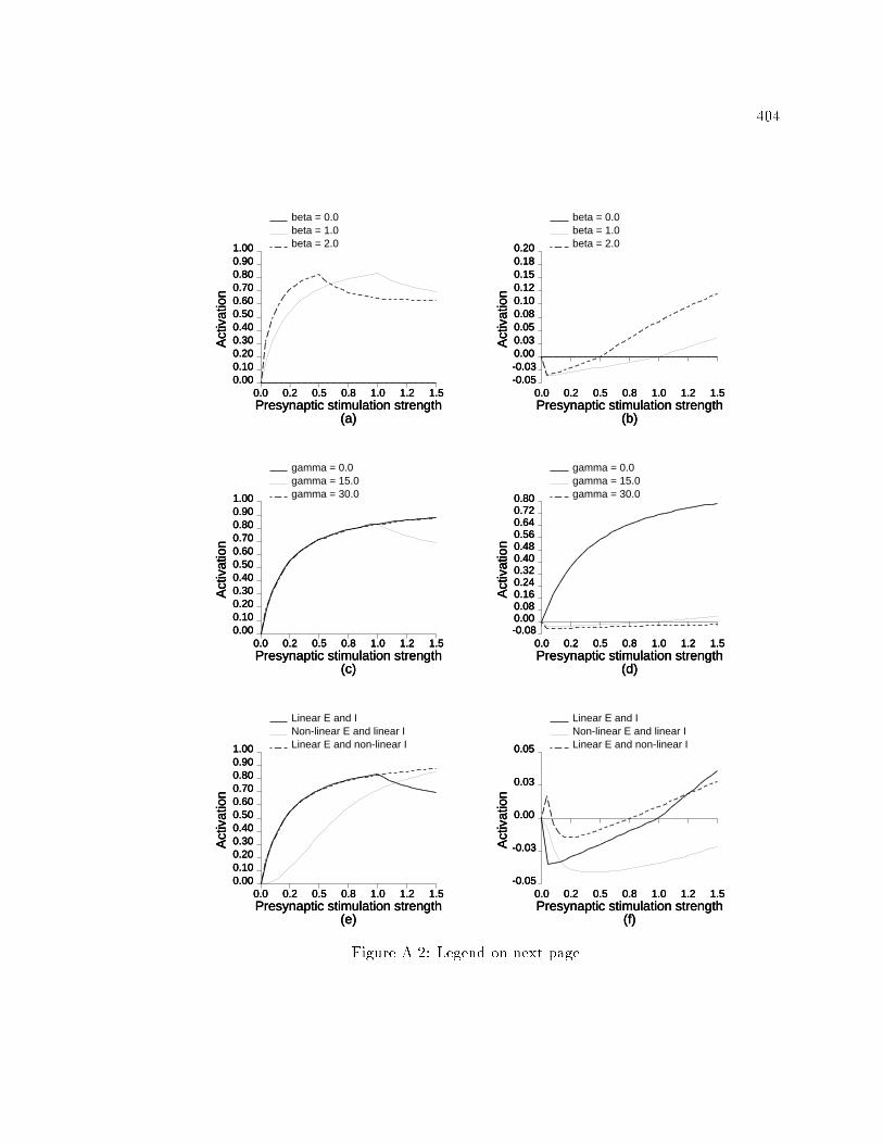
4040.0 0.2 0.5 0.8 1.0 1.2 1.5

0.000.100.200.300.400.500.600.700.800.901.00

Presynaptic stimulation strength(a)

Act

ivat

ion

beta = 0.0

0.0 0.2 0.5 0.8 1.0 1.2 1.5-0.05-0.030.000.030.050.080.100.120.150.180.20

Presynaptic stimulation strength(b)

Act

ivat

ion

beta = 0.0

0.0 0.2 0.5 0.8 1.0 1.2 1.50.000.100.200.300.400.500.600.700.800.901.00

Presynaptic stimulation strength(a)

Act

ivat

ion

beta = 1.0

0.0 0.2 0.5 0.8 1.0 1.2 1.5-0.05-0.030.000.030.050.080.100.120.150.180.20

Presynaptic stimulation strength(b)

Act

ivat

ion

beta = 1.0

0.0 0.2 0.5 0.8 1.0 1.2 1.50.000.100.200.300.400.500.600.700.800.901.00

Presynaptic stimulation strength(a)

Act

ivat

ion

beta = 2.0

0.0 0.2 0.5 0.8 1.0 1.2 1.5-0.05-0.030.000.030.050.080.100.120.150.180.20

Presynaptic stimulation strength(b)

Act

ivat

ion

beta = 2.0

0.0 0.2 0.5 0.8 1.0 1.2 1.50.000.100.200.300.400.500.600.700.800.901.00

Presynaptic stimulation strength(c)

Act

ivat

ion

gamma = 0.0

0.0 0.2 0.5 0.8 1.0 1.2 1.5-0.080.000.080.160.240.320.400.480.560.640.720.80

Presynaptic stimulation strength(d)

Act

ivat

ion

gamma = 0.0

0.0 0.2 0.5 0.8 1.0 1.2 1.50.000.100.200.300.400.500.600.700.800.901.00

Presynaptic stimulation strength(c)

Act

ivat

ion

gamma = 15.0

0.0 0.2 0.5 0.8 1.0 1.2 1.5-0.080.000.080.160.240.320.400.480.560.640.720.80

Presynaptic stimulation strength(d)

Act

ivat

ion

gamma = 15.0

0.0 0.2 0.5 0.8 1.0 1.2 1.50.000.100.200.300.400.500.600.700.800.901.00

Presynaptic stimulation strength(c)

Act

ivat

ion

gamma = 30.0

0.0 0.2 0.5 0.8 1.0 1.2 1.5-0.080.000.080.160.240.320.400.480.560.640.720.80

Presynaptic stimulation strength(d)

Act

ivat

ion

gamma = 30.0

0.0 0.2 0.5 0.8 1.0 1.2 1.50.000.100.200.300.400.500.600.700.800.901.00

Presynaptic stimulation strength(e)

Act

ivat

ion

Linear E and I

0.0 0.2 0.5 0.8 1.0 1.2 1.5-0.05

-0.03

0.00

0.03

0.05

Presynaptic stimulation strength(f)

Act

ivat

ion

Linear E and I

0.0 0.2 0.5 0.8 1.0 1.2 1.50.000.100.200.300.400.500.600.700.800.901.00

Presynaptic stimulation strength(e)

Act

ivat

ion

Non-linear E and linear I

0.0 0.2 0.5 0.8 1.0 1.2 1.5-0.05

-0.03

0.00

0.03

0.05

Presynaptic stimulation strength(f)

Act

ivat

ion

Non-linear E and linear I

0.0 0.2 0.5 0.8 1.0 1.2 1.50.000.100.200.300.400.500.600.700.800.901.00

Presynaptic stimulation strength(e)

Act

ivat

ion

Linear E and non-linear I

0.0 0.2 0.5 0.8 1.0 1.2 1.5-0.05

-0.03

0.00

0.03

0.05

Presynaptic stimulation strength(f)

Act

ivat

ion

Linear E and non-linear I

Figure A.2: Legend on next page.

405Figure A.2: The e�ects of varying �, , input excitation function, and inputinhibition function on the activation equation.Figure on previous page. The initial network synaptic weights are given in Figure 2.8.The activation level of neuron a (left panels) and neuron b (right panels) was determinedusing Equation 2.1. The activation level of the input neuron a was varied from 0 to 1.5.In panels (a) and (b) A = 0:1, B = 1:0, C = 0:05, � 2 f0:0; 1:0; 2:0g, and = 15.In panels (c) and (d) A = 0:1, B = 1:0, C = 0:05, � = 1:0, and 2 f0; 15; 30g. Inpanels (e) and (f) A = 0:1, B = 1:0, C = 0:05, � = 1:0, and = 15. The label \LinearE and I" refers to using Equations 2.2 and 2.3 in Equation 2.1. The label \Non-linear Eand linear I" refers to using Equations 2.3 in Equation 2.1, but Equation 2.2 was replacedby Ej = �Pi[xi]W+ij �2, and the \Linear E and non-linear I" refers to using Equations 2.2in Equation 2.1, but Equation 2.3 was replaced by Ij = Pk[xk]2W�kj . When � = 0, theactivation of neurons a and b is 0.

406Appendix BParameters used in the simulationsof Chapters 3 and 4The parameter values used in the simulations are presented in the followingsections. The notation [a] is de�ned to mean max(0; a). The notation bac is de�ned tomean the largest integer less than or equal to a.B.1 Activation equation parametersThe parameters used for computing the activations were A = 0:1, B = 1:0,C = 0:05, � = 0:1, and = 10. The activation equation for Layer 2 neurons was numericallyintegrated using the Euler method with a time step of 0.013, and the activation levels ofall the neurons were initially set to zero. The network was close to an equilibrium state bytime = 27 (the maximal change in activation level was less than 10�6).During conditioning, the synaptic weight values were updated every 200 time steps.Weights were not changed during RF measurement.B.2 Initial networkThe initial network weights were set to have a coarse receptive �eld topography;nearby neurons were assigned overlapping a�erent excitatory inputs. The model cortical

407layer and the model left and right eye selective input layers had a 1-D ring arrangement.Let model cortical neurons be refered to by the index j 2 f0; � � � ; 41g, and left andright eye selective model input neurons be indexed by l and r, respectively. Then,Z+lj = 0:56 exp �((bic+ p)� i)21:22 !+ 0:2Rlj! ; (B.1)and Z+rj = 0:56 exp �((bic+ p)� i)21:22 !+ 0:2Rrj! ; (B.2)where i = (bj=3c)=2, p 2 f�3;�2;�1; 0; 1; 2; 3g, and l; r = (bic + p) mod 4, and Rlj andRrj are uniformly distributed independent random variables in [0; 1).The initial lateral inhibitory weights were assigned based on the amount of overlapin a�erent pathways to the model cortical neurons. Lateral inhibitory weights betweenmodel cortical neurons j and k, where j; k 2 f0; � � � ; 41g, were computed as follows. Letj 6= k and W�jk = W�kj = 6Xl = 0min �Z+lj ; Z+lk�+ 6Xr = 0min �Z+rj ; Z+rk� : (B.3)Then Z�jk = Z�kj = 0:05W�jkmaxa;b 2 Model cortical layerW�ab : (B.4)The lateral inhibitory pathway weights Z�jj were always �xed at 0.After assigning the initial weights, the network was trained using binocular stimuli(Section B.3), and the resulting network was used for the various \classical" rearing andmodel pharmacological manipulations.B.3 Training and test stimuliDuring NR, the training stimuli were binocular inputs with a range of disparities,and some noise. The input to an eye was a 1-D truncated Gaussian centered at real-valuedpositions in the corresponding model input layer. The model left and right eye selectiveinput neurons were placed at integer positions f0; � � � ; 6g. The inputs were wrapped arounda 1-D ring topology. When monocular input was at position x 2 [0; 7), input layer neuron

408p 2 f0; � � � ; 6g in that eye was assigned activation levelxp = exp ��1:2 ((q + bxc)� x)2�+ (0:01� 0:02Rp) (B.5)where q 2 f�3;�2;�1; 0; 1; 2; 3g, p = (bxc + q) mod 4, and Rp is a uniformlydistributed independent random variable in [0; 1). The noise added to the left andright eyes was independent. If xp < 0:31, it was set to 0. The disparities used weref�2; �4=3; �2=3; 0; 2=3; 4=3; 2g.The 1-D truncated Gaussian input without any noise was used to map themonocular left and right eye RF of the model cortical neurons.B.4 Normal rearing procedureDuring normal rearing, a binocular input with randomly chosen disparityd at a randomly chosen cyclopean position x 2 [0; 7) was presented, where d 2f�2; �4=3; �2=3; 0; 2=3; 4=3; 2g. The disparity and cyclopean position were pickedwith a uniform probability distribution. A binocular input with disparity d at cyclopeanposition x had left eye input at x� d=2 and right eye input at x+ d=2.The network was trained with 1,500,000 presentations of binocular inputs. After1,500,000 input presentations, the network weights and model cortical neuronal RFs werestable. The stability of the network was evaluated by measuring the Euclidean distancebetween the network weight vectors at intervals of 5000 input presentations. After 1,500,000presentations of binocular inputs, the distance between the network weight vectors hadreached an asymptote. With an additional 150,000 binocular input presentations, the meandistance between the a�erent excitatory weight vectors after every 5000 input presentations(de) was was 5:009� 10�2� 1:029� 10�2, the mean distance between the lateral inhibitoryweight vectors after every 5000 input presentations (di) was 5:422� 10�2 � 1:180� 10�2,and the mean distance between the response vector of the neurons to monocular inputsafter every 5000 input presentations (dr) was 1:225� 10�2 � 1:629� 10�3. The Euclideandistance between weight vectors and the response vector between the network before andafter the additional 150,000 binocular input presentations were: De = 1:531 � 10�1 for

409a�erent excitatory weights, Di = 8:637 � 10�2 for lateral inhibitory weights, and Dr =2:958� 10�2 for the monocular responses. Because De=de = 3:046� (150; 000=5000) = 30,Di=di = 1:593� 30, and Dr=dr = 2:415� 30, the network appears to be very stable.B.5 Classical rearing manipulationsTo model MD, the right eye selective model input neurons were stimulated usingthe truncated 1-D Gaussian inputs, and the left eye selective model input neuron l wasactivated by zero mean noise, (0:01� 0:02Rl), where Rl 2 [0; 1) is a uniformly distributedindependent random variable. The network was trained with 75,000 monocular inputs.After 75,000 presentations of monocular inputs to the right eye, the left eye alonewas stimulated by 50,000 presentations of monocular inputs to simulate RS. The left eyeselective model input neurons were stimulated using the truncated 1-D Gaussian inputs,and the right eye selective model input neuron r was activated by zero mean noise,(0:01� 0:02Rr), where Rr 2 [0; 1) is a uniformly distributed independent random variable.To model ST, the right eye selective model input neurons or the left eye selectivemodel input neurons were stimulated using the truncated 1-D Gaussian inputs, and theunstimulated eye selective model input neuron m was activated by zero mean noise,(0:01�0:02Rm), where Rm 2 [0; 1) is a uniformly distributed independent random variable.The network was trained with 500,000 strabismic inputs.During BD, left eye and right eye selective model input neurons were activatedby zero mean noise. Left eye selective model input input neuron l was activated by(0:01�0:02Rl), and right eye selective model input neuron r was activated by (0:01�0:02Rl),where Rl;Rr 2 [0; 1) are uniformly distributed independent random variables. The networkwas trained with 5,000,000 input presentations.Following MD, ST, and BD, the network was trained with 500,000 presentationsof binocular inputs used for normal rearing, to model RE.

410B.6 Parameters for synaptic plasticity rulesThe parameters used in the EXIN lateral inhibitory plasticity rule were� = 0:00505, G(xi) = [([xi])2 + N1], and Q(xj) = min(0:2; 3[xj]). The parameters usedin the EXIN a�erent excitatory plasticity rule were � = 0:0025, F(xj) = [([xj])2+N2], andH(xi) = [xi].N1 and N2 were zero-mean noise, whereNi = (0:0001�0:0002Ri), where i 2 f1; 2g,and Ri 2 [0; 1) is a uniformly distributed independent random variable. Noise in the modelinput and cortical neurons was important in modeling the e�ects of chronic binoculardeprivation (see Chapter 3, Section 3.3.5).B.7 Parameters for aspeci�c action of pharmacologicalinfusionIn these simulations, all the model cortical neurons were pharmacologically treated.APV strength was varied by using ! = 0:6 and 0:2 in Equation 4.6, and muscimol strengthwas varied by using = = 0:05 and 0:1 in Equation 4.7 to obtain the simulation resultspresented in Figures 4.3 and 4.5, respectively.For the results in Figure 4.4, lateral inhibitory learning alone was enabled (� = 0),and ! = 0:6 was used in Equation 4.6. For the results in Figure 4.6, = = 0:05 was used inEquation 4.7 with lateral inhibitory and a�erent excitatory plasticity using the parametersin Section B.6. The network was trained with 500,000 binocular input presentations.B.8 E�ects of pharmacological infusionTo model MD with pharmacological infusion, the right eye selective model inputneurons were stimulated using the truncated 1-D Gaussian inputs, and the left eye selectivemodel input neuron l was activated by zero mean noise, (0:01�0:02Rl), whereRl 2 [0; 1) is auniformly distributed independent random variable, and model cortical neurons f12; � � � ; 30gwere treated with an equal concentration of model APV or muscimol. OD after MD wasmeasured at a residual APV or muscimol concentration of half the strength of the APV or

411muscimol used during MD, or with no residual APV or muscimol. The network was trainedwith 75,000 monocular inputs.To model NR with pharmacological infusion, binocular inputs were used to trainthe network with all model cortical neurons equally a�ected by the pharmacological infusion.The network was trained with 5,000,000 binocular inputs.B.8.1 APV infusionTo study the e�ects of the amount of a�erent excitatory plasticity and APVconcentration during MD, ! was assigned values 0.9, 0.8, and 0.7, and the a�erent excitatoryplasticity rate � was multiplied by a factor of 0, 0.35, and 0.70 (Figure 4.11) in a�erentexcitatory pathways to the APV-treated neurons.To determine the role of cortical responsiveness on RF width and responsivenessafter NR with APV, ! was varied through 1, 0.325, and 0.1, and the a�erent excitatoryplasticity rate in pathways to the model APV-a�ected neurons was zero. All the modelcortical neurons were a�ected by model APV (Figure 4.13).B.8.2 Muscimol infusionTo study the e�ects of the amount of lateral inhibitory plasticity and muscimolconcentration during MD, = was assigned the values 0.05, 0.1, and 0.2, and the a�erentexcitatory plasticity rate � was not changed (Figure 4.12). The lateral inhibitory plasticityrate � was multiplied by a factor of 0; 0:5; 1:0 in lateral inhibitory pathways to neuronsa�ected by muscimol.To determine the role of cortical responsiveness on RF width and responsivenessafter NR with muscimol, = was varied through 0, 0.2, and 0.4. The lateral inhibitory anda�erent excitatory plasticity rules used the parameters in Section B.6 (Figure 4.13).

412Appendix CParameters used in the simulationsof Chapter 5The parameter values used to simulate the three models were chosen as follows.The notation [a] is de�ned to mean max(0; a).C.1 Parameters for the EXIN model simulationsThe following parameters were used in all the EXIN simulations. To compute theinitial weights, �� = 1:41, = 0:2, �� = 0:01, = 0:45, and �i = 0 were used.The parameters used for computing the activations were A = 0:2, B = 2, C = 0:3,� = 0:1, and = 0:2. The activation equation for Layer 2 neurons were numericallyintegrated using the Euler method with a time step of 0.2. The initial activation level ofall the neurons was zero. The simulations were stopped at time = 110. At time = 110, thenetwork was close to an equilibrium state by time = 110; the maximal change in Layer 2neuronal activation at that point was less than 10�5.In the simulation, the weights were modi�ed after the Layer 2 activations reachedequilibrium on each input presentation. To compute the lateral inhibitory weight changes,parameters � = 0:2, G(a) = [a], and Q(a) = 3[a] were used. To compute the a�erentexcitatory weight changes, � = 0:0016, F(a) = [a], and H(a) = 0:4[a] were used. When the

413a�erent excitatory synaptic plasticity was enabled, the initially zero a�erent weights arenot changed. This was done to speedup convergence of the a�erent weights.C.1.1 Parameters for the activation equationThe parameters of the activation equation were chosen so that the network gavea distributed activation response to an input, instead of a winner-take-all response.At equilibrium, ddtxpq = 0 and the activation levels of Layer 2 neurons are givenby xpq = �BEpq � CIpqA + �Epq + Ipq (C.1)Because Equation 5.3 is a shunting equation, xpq(t) 2 [�C;B] if xpq(0) 2 [�C;B],for all t � 0 (Cohen & Grossberg, 1983). Thus, B is the maximum activation level and �Cis the minimum activation level of Layer 2 neurons. The constant A determines the passivedecay rate.Increasing � is equivalent to increasing the input strength. As � is increased,the activation levels of neurons receiving large excitation increase and the activation levelsof neurons receiving zero or very weak excitation are suppressed. This property of theshunting equation is shown in Figure C.1a. Note that as � is increased (by a factor of 21),the Layer 2 activation pro�le expands very little. The activation level of neurons receivingstrong excitation increases, and the activation level of neurons receiving very weak or zeroexcitation is further suppressed. As is increased, the activation levels of neurons �rstdecrease and the response pro�le becomes narrower. At very large values of , the networkbehaves in a winner-take-all manner (Figure C.1b).Increasing B is similar to increasing �. This property of the shunting equation isshown in Figure C.1c. Increasing C causes the Layer 2 activation pro�le to shift downwards.This property of the shunting equation is shown in Figure C.1d. At very large values of C,the network behaves in a winner-take-all manner.The parameters were chosen so that none of the terms in the shunting equation(Equation 5.3) dominates the others. With such a choice, changes in the weights resultedin signi�cant changes in RF size, shape, and responsiveness. The desirable dynamic

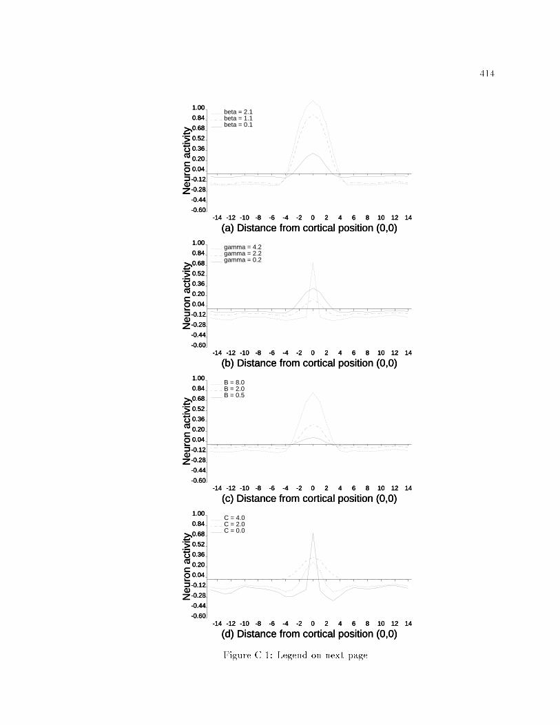
414-14 -12 -10 -8 -6 -4 -2 0 2 4 6 8 10 12 14

-0.60

-0.44

-0.28

-0.12

0.04

0.20

0.36

0.52

0.68

0.84

1.00

beta = 0.1

Neu

ron

activ

ity

(a) Distance from cortical position (0,0)-14 -12 -10 -8 -6 -4 -2 0 2 4 6 8 10 12 14

-0.60

-0.44

-0.28

-0.12

0.04

0.20

0.36

0.52

0.68

0.84

1.00

beta = 1.1

Neu

ron

activ

ity

(a) Distance from cortical position (0,0)-14 -12 -10 -8 -6 -4 -2 0 2 4 6 8 10 12 14

-0.60

-0.44

-0.28

-0.12

0.04

0.20

0.36

0.52

0.68

0.84

1.00beta = 2.1

Neu

ron

activ

ity

(a) Distance from cortical position (0,0)

-14 -12 -10 -8 -6 -4 -2 0 2 4 6 8 10 12 14-0.60

-0.44

-0.28

-0.12

0.04

0.20

0.36

0.52

0.68

0.84

1.00

gamma = 0.2

Neu

ron

activ

ity

(b) Distance from cortical position (0,0)-14 -12 -10 -8 -6 -4 -2 0 2 4 6 8 10 12 14

-0.60

-0.44

-0.28

-0.12

0.04

0.20

0.36

0.52

0.68

0.84

1.00

gamma = 2.2

Neu

ron

activ

ity

(b) Distance from cortical position (0,0)-14 -12 -10 -8 -6 -4 -2 0 2 4 6 8 10 12 14

-0.60

-0.44

-0.28

-0.12

0.04

0.20

0.36

0.52

0.68

0.84

1.00gamma = 4.2

Neu

ron

activ

ity

(b) Distance from cortical position (0,0)

-14 -12 -10 -8 -6 -4 -2 0 2 4 6 8 10 12 14-0.60

-0.44

-0.28

-0.12

0.04

0.20

0.36

0.52

0.68

0.84

1.00

B = 0.5

Neu

ron

activ

ity

(c) Distance from cortical position (0,0)-14 -12 -10 -8 -6 -4 -2 0 2 4 6 8 10 12 14

-0.60

-0.44

-0.28

-0.12

0.04

0.20

0.36

0.52

0.68

0.84

1.00

B = 2.0

Neu

ron

activ

ity

(c) Distance from cortical position (0,0)-14 -12 -10 -8 -6 -4 -2 0 2 4 6 8 10 12 14

-0.60

-0.44

-0.28

-0.12

0.04

0.20

0.36

0.52

0.68

0.84

1.00B = 8.0

Neu

ron

activ

ity

(c) Distance from cortical position (0,0)

-14 -12 -10 -8 -6 -4 -2 0 2 4 6 8 10 12 14-0.60

-0.44

-0.28

-0.12

0.04

0.20

0.36

0.52

0.68

0.84

1.00

C = 0.0

Neu

ron

activ

ity

(d) Distance from cortical position (0,0)-14 -12 -10 -8 -6 -4 -2 0 2 4 6 8 10 12 14

-0.60

-0.44

-0.28

-0.12

0.04

0.20

0.36

0.52

0.68

0.84

1.00

C = 2.0

Neu

ron

activ

ity

(d) Distance from cortical position (0,0)-14 -12 -10 -8 -6 -4 -2 0 2 4 6 8 10 12 14

-0.60

-0.44

-0.28

-0.12

0.04

0.20

0.36

0.52

0.68

0.84

1.00C = 4.0

Neu

ron

activ

ity

(d) Distance from cortical position (0,0)Figure C.1: Legend on next page.

415Figure C.1: Behavior of the EXIN network as a function of activation equationparameters.Figure on previous page. The equilibrium activation level of a one-dimensional cross-sectionof Layer 2: neurons (0;�15){(0; 14), in response to input at (0; 0). The EXIN network usedwas obtained after training with 25,000 normal inputs with only lateral inhibitory synapticplasticity enabled. The network reached a stable state by time 110. (a) The parameter �in Equation 3 is varied by a factor of 21, yet the width of the response curve increases byonly a small amount. (b) When the parameter in Equation 3 is increased from 0.2 to 4.2,the network exhibits winner-take-all behavior. (c) The parameter B in Equation 3 is variedby a factor of 16, yet the width of the response curve increases by only a small amount.(d) When the parameter C in Equation 3 is set to 4, the network exhibits winner-take-allbehavior. When C is zero, the neurons have non-negative activation levels.RF changes can be obtained for a wide range of choices for the parameters in the shuntingequation, as long as no term dominates the others.The stability of the activation equation was established empirically. The activationequation was computed using the Euler method. Care was taken to ensure that the stepsize and the number of steps resulted in convergence and that there were no oscillations.Figure C.2 shows the activation as a function of time of 30 Layer 2 neurons in response toinput at (0; 0).Figures C.3b{c show that the activation equation converged during the trainingphase. During the training phase, the sum over all the Layer 2 neurons of the absolutechange in activation level, at each step of the Euler method, is averaged over training inputpresentation at intervals of 100 input presentations.Figures C.3b{c demonstrate the convergence of the shunting equation duringthe training phase using normal stimuli and scotoma stimuli, respectively, in the EXINnetwork with only lateral inhibitory synaptic plasticity enabled. The activation equationalso converged to a �xed point during the other types of conditioning; the maximal changein Layer 2 neuronal activation was less than 10�5.C.1.2 Parameters for the learning equationsThe rates of weight change in the EXIN synaptic plasticity rules were chosenso that spurious correlations do not produce large changes in the connection weights;

416

0 10 20 30 40 50 60 70 80 90 100 110-0.30-0.22-0.14-0.060.020.100.180.260.340.420.50

Neu

ron

activ

ity

Time0 10 20 30 40 50 60 70 80 90 100 110

-0.30-0.22-0.14-0.060.020.100.180.260.340.420.50

Neu

ron

activ

ity

Time0 10 20 30 40 50 60 70 80 90 100 110

-0.30-0.22-0.14-0.060.020.100.180.260.340.420.50

Neu

ron

activ

ity

Time0 10 20 30 40 50 60 70 80 90 100 110

-0.30-0.22-0.14-0.060.020.100.180.260.340.420.50

Neu

ron

activ

ity

Time0 10 20 30 40 50 60 70 80 90 100 110

-0.30-0.22-0.14-0.060.020.100.180.260.340.420.50

Neu

ron

activ

ity

Time0 10 20 30 40 50 60 70 80 90 100 110

-0.30-0.22-0.14-0.060.020.100.180.260.340.420.50

Neu

ron

activ

ity

Time0 10 20 30 40 50 60 70 80 90 100 110

-0.30-0.22-0.14-0.060.020.100.180.260.340.420.50

Neu

ron

activ

ity

Time0 10 20 30 40 50 60 70 80 90 100 110

-0.30-0.22-0.14-0.060.020.100.180.260.340.420.50

Neu

ron

activ

ity

Time0 10 20 30 40 50 60 70 80 90 100 110

-0.30-0.22-0.14-0.060.020.100.180.260.340.420.50

Neu

ron

activ

ity

Time0 10 20 30 40 50 60 70 80 90 100 110

-0.30-0.22-0.14-0.060.020.100.180.260.340.420.50

Neu

ron

activ

ity

Time0 10 20 30 40 50 60 70 80 90 100 110

-0.30-0.22-0.14-0.060.020.100.180.260.340.420.50

Neu

ron

activ

ity

Time0 10 20 30 40 50 60 70 80 90 100 110

-0.30-0.22-0.14-0.060.020.100.180.260.340.420.50

Neu

ron

activ

ity

Time0 10 20 30 40 50 60 70 80 90 100 110

-0.30-0.22-0.14-0.060.020.100.180.260.340.420.50

Neu

ron

activ

ity

Time0 10 20 30 40 50 60 70 80 90 100 110

-0.30-0.22-0.14-0.060.020.100.180.260.340.420.50

Neu

ron

activ

ity

Time0 10 20 30 40 50 60 70 80 90 100 110

-0.30-0.22-0.14-0.060.020.100.180.260.340.420.50

Neu

ron

activ

ity

Time0 10 20 30 40 50 60 70 80 90 100 110

-0.30-0.22-0.14-0.060.020.100.180.260.340.420.50

Neu

ron

activ

ity

Time0 10 20 30 40 50 60 70 80 90 100 110

-0.30-0.22-0.14-0.060.020.100.180.260.340.420.50

Neu

ron

activ

ity

Time0 10 20 30 40 50 60 70 80 90 100 110

-0.30-0.22-0.14-0.060.020.100.180.260.340.420.50

Neu

ron

activ

ity

Time0 10 20 30 40 50 60 70 80 90 100 110

-0.30-0.22-0.14-0.060.020.100.180.260.340.420.50

Neu

ron

activ

ity

Time0 10 20 30 40 50 60 70 80 90 100 110

-0.30-0.22-0.14-0.060.020.100.180.260.340.420.50

Neu

ron

activ

ity

Time0 10 20 30 40 50 60 70 80 90 100 110

-0.30-0.22-0.14-0.060.020.100.180.260.340.420.50

Neu

ron

activ

ity

Time0 10 20 30 40 50 60 70 80 90 100 110

-0.30-0.22-0.14-0.060.020.100.180.260.340.420.50

Neu

ron

activ

ity

Time0 10 20 30 40 50 60 70 80 90 100 110

-0.30-0.22-0.14-0.060.020.100.180.260.340.420.50

Neu

ron

activ

ity

Time0 10 20 30 40 50 60 70 80 90 100 110

-0.30-0.22-0.14-0.060.020.100.180.260.340.420.50

Neu

ron

activ

ity

Time0 10 20 30 40 50 60 70 80 90 100 110

-0.30-0.22-0.14-0.060.020.100.180.260.340.420.50

Neu

ron

activ

ity

Time0 10 20 30 40 50 60 70 80 90 100 110

-0.30-0.22-0.14-0.060.020.100.180.260.340.420.50

Neu

ron

activ

ity

Time0 10 20 30 40 50 60 70 80 90 100 110

-0.30-0.22-0.14-0.060.020.100.180.260.340.420.50

Neu

ron

activ

ity

Time0 10 20 30 40 50 60 70 80 90 100 110

-0.30-0.22-0.14-0.060.020.100.180.260.340.420.50

Neu

ron

activ

ity

Time0 10 20 30 40 50 60 70 80 90 100 110

-0.30-0.22-0.14-0.060.020.100.180.260.340.420.50

Neu

ron

activ

ity

Time0 10 20 30 40 50 60 70 80 90 100 110

-0.30-0.22-0.14-0.060.020.100.180.260.340.420.50

Neu

ron

activ

ity

TimeFigure C.2: Activation curves in the EXIN network after whole-�eld stimulation.The activation level of a one-dimensional cross-section of Layer 2: neurons (0;�15){(0; 14),in response to input at (0; 0) in the EXIN network after training with 25,000 normalinputs with only lateral inhibitory synaptic plasticity enabled. The network equilibrates bytime 110. Note that some neurons that were active during the initial stages are eventuallysuppressed.

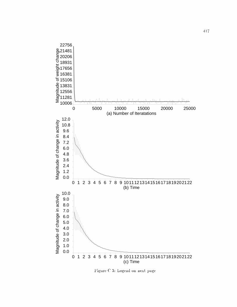
4170 5000 10000 15000 20000 25000

1000611281125561383115106163811765618931202062148122756

Mag

nitu

de o

f wei

ght c

hang

e

(a) Number of Iteratations

0 1 2 3 4 5 6 7 8 9 101112131415161718192021220.01.22.43.64.86.07.28.49.610.812.0

Mag

nitu

de o

f cha

nge

in a

ctiv

ity

(b) Time

0 1 2 3 4 5 6 7 8 9 101112131415161718192021220.01.02.03.04.05.06.07.08.09.0

10.0

Mag

nitu

de o

f cha

nge

in a

ctiv

ity

(c) TimeFigure C.3: Legend on next page.

418Figure C.3: Stability of the EXIN network with lateral inhibitory synapticplasticity alone.Figure on previous page. The jagged line in panel (a) shows the total change in the lateralinhibitory pathway weights in the EXIN network, after 100 presentations of normal stimuli,over the course of 25,000 normal input presentations. The total change is obtained bysumming the magnitude of the weight changes at intervals of 100 input presentations, overall the lateral inhibitory pathways. The smooth line in panel (a) is the nonlinear leastsquares �t of the data using the Marquardt-Levenberg algorithm. The non-linear functionis a� exp(�b � iteration number) + c. The best �t parameters are a = 53864:9� 5665:23,b = 1:490� 0:098, and c = 10648:6� 18:26. The sum over all Layer 2 neurons, of themagnitude of change in the activation level at each step in the Euler method for solvingthe activation equation (Equation 3), is averaged over input presentations at intervals of100 during normal conditioning (b), and during scotoma conditioning (c). The vertical linesin (b,c) represent the standard deviation.only consistent correlations over several input presentations produce signi�cant changes inconnection weights. Figure C.3a plots the sum of the absolute weight change in all lateralinhibitory pathways after every 100 training input presentations, in the EXIN network withonly lateral inhibitory synaptic plasticity enabled during normal conditioning.During the normal conditioning phase, the EXIN network simulations with lateralinhibitory plasticity alone, with a�erent excitatory plasticity alone, and with both lateralinhibitory and a�erent excitatory plasticity were trained until the sum of the absolute weightchange in plastic pathways after every 100 input presentations reached an asymptote.The Euclidean distance between the network weight vector before and after anadditional 10; 000 training steps (D), was compared with the average Euclidean distancebetween the network weight vectors at successive intervals of 100 training steps (d). Withlateral inhibitory synaptic plasticity alone D = 24:599667, d = 15:691748 � 0:251141(D=d = 1:568), with a�erent excitatory synaptic plasticity alone D = 0:451494 and d =0:050187� 0:000005 (D=d = 8:996), and with both synaptic plasticity rules D = 0:699971and d = 0:052240 � 0:000005 (D=d = 13:399) for the a�erent excitatory weights andD = 19:516132 and d = 12:193612 � 0:194959 (D=d = 1:601) for the lateral inhibitoryweights. In all cases D=d � 10; 000=100 = 100, suggesting that the networks are close toan equilibrium point.

419C.2 Parameters for the LISSOM simulationsTo compute the initial weights in the LISSOM simulations �� = 1, �e = 1:41,�i = 2:36, �� = 0:01, �e = 0:1, and �i = 0:001 were used.The parameters used for computing the activations were � = 0:8, e = 1:8,and i = 1:3. During training and testing LISSOM with only a�erent excitatory, lateralexcitatory, or lateral inhibitory synaptic plasticity enabled, the activation equation wasclose to an equilibrium state by 30 iterations. The initial value of the activation level waszero for all neurons.The weights were modi�ed after the Layer 2 activations reached equilibriumon each input presentation. To compute the weight changes, parameters �� = 0:01,�e = 0:0005, and �i = 0:01 were used. The weights, which were initially set to zero,were not changed. Without this restriction, normalization would cause all the weights tobecome very small.C.2.1 Parameters for the activation equationThe parameters of the activation equation were chosen so that the network gavea distributed activation response to its inputs. The LISSOM activation equation rapidlyconverges (Sirosh & Miikkulainen, 1994b). The parameters were chosen so that none of theterms in the LISSOM activation equation (Equation 5.14) dominated the others. In all theLISSOM simulations, the maximal change in Layer 2 neuronal activation was less than 10�5when the activation equation computation was stopped.C.2.2 Parameters for the learning equationsThe rates of weight change in the LISSOM synaptic plasticity rules were chosen sothat changes in the connection weights because of spurious correlations gets averaged overa large number of input presentations.In the initial normal conditioning phase, the networks were trained until theamount of weight change reached an asymptote (the criterion is the same as for the EXINsimulations).

420With an additional 10,000 normal training inputs, D = 0:219775, d = 0:017082�0:000001 (D=d = 12:866) with only lateral inhibitory synaptic plasticity enabled, D =2:256291 and d = 0:620959� 0:000422 (D=d = 3:634) with only lateral excitatory synapticplasticity enabled, and D = 3:065377 and d = 0:795790�0:000873 (D=d = 3:852) with onlya�erent excitatory synaptic plasticity enabled. D=d � 100, suggesting that the networksare close to an equilibrium state.C.3 Parameters for the adaptation model simulationsTo compute the initial weights in the inhibition-dominant adaptation model,parameters �� = 2:13, �e = 1:19, �i = 3:53, �� = 0:01, �e = 0:1, and �i = 0:001were used.In the adaptation model with no lateral interaction, the lateral excitatory andlateral inhibitory weights were set to zero. The excitation-dominant adaptation model hadthe same weights as the inhibition-dominant adaptation model. The initial adaptation levelwas 0. In the inhibition-dominant adaptation model, the parameters used for computingthe activations were A = 0:2, B = 2, C = 0:3, �� = 1, �e = 0:1, and = 8. The activationequations for Layer 2 neurons were numerically integrated using the Euler method with atime step of 1=75. The network was very close to an equilibrium state by time = 15; themaximal change in Layer 2 neuronal activation was less than 10�5.In the adaptation model with no lateral interaction, the activation equation wassolved analytically. With no lateral interactions, the activation equation equilibrates whenxpq = BEpqA + Epq ; (C.2)where Epq = ���(i;j)2Layer 1[xij ]Z+ij;pq, A = 0:2, B = 2, and �� = 1.In the excitation-dominant adaptation model, A = 0:2, B = 2, C = 0:3, �� = 0:1,�e = 0:01, and = 0. The activation equations for Layer 2 neurons were numericallyintegrated using the Euler method with a time step of 1=75. The network reached anequilibrium state by time = 15.

421In all three adaptation models, the initial activation level of all neurons waszero. The adaptation threshold parameters were modi�ed after the Layer 2 activationsreached equilibrium on each input presentation. To compute the changes in the adaptationthreshold, � = 0:0004, � = 0:3, and � = 15 were used in the inhibition-dominant adaptationmodel. In the adaptation model without lateral interaction and the excitation-dominantadaptation model, � = 0:0004, � = 0:3, and � = 2 were used.C.3.1 Parameters for the activation equationThe shunting equation (Equation 5.16) was used in the adaptation models.However, the activation equation in the adaptation models di�ers from the activationequation in the EXIN model in two respects: (1) the presence of lateral excitation in theadaptation model; (2) the threshold in computing lateral excitation and lateral inhibition.The parameters of the activation equation were chosen so that the network gave a distributedresponse to its inputs.The activation equation in the adaptation model behaved similarly to theactivation equation in the EXIN model. To make the model inhibition-dominant(excitation-dominant) the constant �e was chosen to be much smaller (larger) than theconstant . As neurons are habituated they propagate less lateral excitation and lateralinhibition.In all the adaptation model simulations, the maximal change in Layer 2 neuronalactivation was less than 10�6 when the activation equation computation was stopped. Theadaptation model with no lateral interaction had a unique �xed point (Equation C.2).C.3.2 Parameters for the adaptation equationThe rate of the adaptation equation was chosen so that the adaptation level ofneurons depended on neuronal activation over a large number of input presentations. Inthe initial normal conditioning phase, the networks were trained until the amount of weightchange reached an asymptote (the criterion is the same as for the EXIN simulations).With an additional 10,000 normal training inputs, D = 0:229360, d = 0:088466�0:000293 (D=d = 2:593) in the network with no lateral interaction, D = 0:113066

422and d = 0:032176 � 0:000004 (D=d = 3:514) in the inhibition dominant network, andD = 0:131278 and d = 0:026841 � 0:000017 (D=d = 4:891) in the excitation dominantnetwork. In the all these networks D=d � 100, suggesting that the networks are close toan equilibrium point.C.4 Parameters for generating the inputs for the simulationsIn generating the input patterns for training, the kernel K wasK = 266664 0:55 0:74 0:550:74 1:00 0:740:55 0:74 0:55 377775 :The probability, �, that the input at each position is 1 was 0.02.C.5 Parameters for RF measurementsThe threshold � used for RF measurements was chosen as follows. The activationlevel of Layer 2 neurons was scaled relative to 1:25 times the maximal response of Layer 2neuron to test stimuli, in the network obtained after the initial whole-�eld stimulation. Inall the simulations, � = 0:01.C.6 Conditioning procedureAfter setting the initial weights in the models, the equilibrium state of the weightsor the adaptation levels with respect to the inputs used in the simulations was obtainedby training the networks with 25,000 presentations of normal stimuli, except for the EXINnetwork with a�erent synaptic plasticity, and the EXIN network with a�erent and lateralinhibitory synaptic plasticity, which were trained with 50,000 presentations of normalstimuli, and the LISSOM network with only lateral excitatory synaptic plasticity, whichwas trained with 75,000 presentations of normal stimuli. For scotoma and complementaryscotoma conditioning and for reversing the e�ects of scotoma and complementary scotoma

423conditioning, 5000 presentations of the appropriate stimulus were used, except for the EXINnetwork with a�erent synaptic plasticity and the EXIN network with a�erent and lateralinhibitory synaptic plasticity, which were trained with 50,000 input presentations, and theLISSOM network with only lateral excitatory synaptic plasticity, which was trained with25,000 input presentations. In complementary scotoma conditioning, the complementaryscotoma stimuli were alternated.

424Appendix DParameters used in the simulationsof Chapter 6The parameter values used in the simulations are presented in the followingsections. The notation [a] is de�ned to mean max(0; a), and the notation bac is de�nedto mean the largest integer less than or equal to a. In all the simulations, the weights weremodi�ed after the Layer 2 activations were close to equilibrium on each input presentation.D.1 Parameters for the activation equationThe parameters used for computing the activations were A = 0:2, B = 2:0,C = 0:3, � = 0:01, and = 1:3. The activation equations for Layer 2 neurons werenumerically integrated using the Euler method with a time step of 1=1200, and theactivations of all the neurons were initially set to zero. The network was close to anequilibrium state by time = 14.The parameters of the activation equation were chosen so that the network gavea distributed activation response to an input, instead of a winner-take-all response.Because Equation 6.8 is a shunting equation, xpq(t) 2 [�C;B] if xpq(0) 2 [�C;B],t � 0 (Cohen & Grossberg, 1983). Thus, B is the maximum activation level and �C is theminimum activation level of Layer 2 neurons. The constant A determines the passive decay

4250 1 2 3 4 5 6 7 8 9 10 11 12 13 14

-0.15

-0.11

-0.07

-0.03

0.01

0.05

0.09

0.13

0.17

0.21

0.25N

euro

n ac

tivity

Time0 1 2 3 4 5 6 7 8 9 10 11 12 13 14

-0.15

-0.11

-0.07

-0.03

0.01

0.05

0.09

0.13

0.17

0.21

0.25N

euro

n ac

tivity

Time0 1 2 3 4 5 6 7 8 9 10 11 12 13 14

-0.15

-0.11

-0.07

-0.03

0.01

0.05

0.09

0.13

0.17

0.21

0.25N

euro

n ac

tivity

Time0 1 2 3 4 5 6 7 8 9 10 11 12 13 14

-0.15

-0.11

-0.07

-0.03

0.01

0.05

0.09

0.13

0.17

0.21

0.25N

euro

n ac

tivity

Time0 1 2 3 4 5 6 7 8 9 10 11 12 13 14

-0.15

-0.11

-0.07

-0.03

0.01

0.05

0.09

0.13

0.17

0.21

0.25N

euro

n ac

tivity

Time0 1 2 3 4 5 6 7 8 9 10 11 12 13 14

-0.15

-0.11

-0.07

-0.03

0.01

0.05

0.09

0.13

0.17

0.21

0.25N

euro

n ac

tivity

Time0 1 2 3 4 5 6 7 8 9 10 11 12 13 14

-0.15

-0.11

-0.07

-0.03

0.01

0.05

0.09

0.13

0.17

0.21

0.25N

euro

n ac

tivity

Time0 1 2 3 4 5 6 7 8 9 10 11 12 13 14

-0.15

-0.11

-0.07

-0.03

0.01

0.05

0.09

0.13

0.17

0.21

0.25N

euro

n ac

tivity

Time0 1 2 3 4 5 6 7 8 9 10 11 12 13 14

-0.15

-0.11

-0.07

-0.03

0.01

0.05

0.09

0.13

0.17

0.21

0.25N

euro

n ac

tivity

Time0 1 2 3 4 5 6 7 8 9 10 11 12 13 14

-0.15

-0.11

-0.07

-0.03

0.01

0.05

0.09

0.13

0.17

0.21

0.25N

euro

n ac

tivity

Time0 1 2 3 4 5 6 7 8 9 10 11 12 13 14

-0.15

-0.11

-0.07

-0.03

0.01

0.05

0.09

0.13

0.17

0.21

0.25N

euro

n ac

tivity

Time0 1 2 3 4 5 6 7 8 9 10 11 12 13 14

-0.15

-0.11

-0.07

-0.03

0.01

0.05

0.09

0.13

0.17

0.21

0.25N

euro

n ac

tivity

Time0 1 2 3 4 5 6 7 8 9 10 11 12 13 14

-0.15

-0.11

-0.07

-0.03

0.01

0.05

0.09

0.13

0.17

0.21

0.25N

euro

n ac

tivity

Time0 1 2 3 4 5 6 7 8 9 10 11 12 13 14

-0.15

-0.11

-0.07

-0.03

0.01

0.05

0.09

0.13

0.17

0.21

0.25N

euro

n ac

tivity

Time0 1 2 3 4 5 6 7 8 9 10 11 12 13 14

-0.15

-0.11

-0.07

-0.03

0.01

0.05

0.09

0.13

0.17

0.21

0.25N

euro

n ac

tivity

Time0 1 2 3 4 5 6 7 8 9 10 11 12 13 14

-0.15

-0.11

-0.07

-0.03

0.01

0.05

0.09

0.13

0.17

0.21

0.25N

euro

n ac

tivity

Time0 1 2 3 4 5 6 7 8 9 10 11 12 13 14

-0.15

-0.11

-0.07

-0.03

0.01

0.05

0.09

0.13

0.17

0.21

0.25N

euro

n ac

tivity

Time0 1 2 3 4 5 6 7 8 9 10 11 12 13 14

-0.15

-0.11

-0.07

-0.03

0.01

0.05

0.09

0.13

0.17

0.21

0.25N

euro

n ac

tivity

Time0 1 2 3 4 5 6 7 8 9 10 11 12 13 14

-0.15

-0.11

-0.07

-0.03

0.01

0.05

0.09

0.13

0.17

0.21

0.25N

euro

n ac

tivity

Time0 1 2 3 4 5 6 7 8 9 10 11 12 13 14

-0.15

-0.11

-0.07

-0.03

0.01

0.05

0.09

0.13

0.17

0.21

0.25N

euro

n ac

tivity

Time0 1 2 3 4 5 6 7 8 9 10 11 12 13 14

-0.15

-0.11

-0.07

-0.03

0.01

0.05

0.09

0.13

0.17

0.21

0.25N

euro

n ac

tivity

Time0 1 2 3 4 5 6 7 8 9 10 11 12 13 14

-0.15

-0.11

-0.07

-0.03

0.01

0.05

0.09

0.13

0.17

0.21

0.25N

euro

n ac

tivity

Time0 1 2 3 4 5 6 7 8 9 10 11 12 13 14

-0.15

-0.11

-0.07

-0.03

0.01

0.05

0.09

0.13

0.17

0.21

0.25N

euro

n ac

tivity

Time0 1 2 3 4 5 6 7 8 9 10 11 12 13 14

-0.15

-0.11

-0.07

-0.03

0.01

0.05

0.09

0.13

0.17

0.21

0.25N

euro

n ac

tivity

Time0 1 2 3 4 5 6 7 8 9 10 11 12 13 14

-0.15

-0.11

-0.07

-0.03

0.01

0.05

0.09

0.13

0.17

0.21

0.25N

euro

n ac

tivity

Time0 1 2 3 4 5 6 7 8 9 10 11 12 13 14

-0.15

-0.11

-0.07

-0.03

0.01

0.05

0.09

0.13

0.17

0.21

0.25N

euro

n ac

tivity

Time0 1 2 3 4 5 6 7 8 9 10 11 12 13 14

-0.15

-0.11

-0.07

-0.03

0.01

0.05

0.09

0.13

0.17

0.21

0.25N

euro

n ac

tivity

Time0 1 2 3 4 5 6 7 8 9 10 11 12 13 14

-0.15

-0.11

-0.07

-0.03

0.01

0.05

0.09

0.13

0.17

0.21

0.25N

euro

n ac

tivity

Time0 1 2 3 4 5 6 7 8 9 10 11 12 13 14

-0.15

-0.11

-0.07

-0.03

0.01

0.05

0.09

0.13

0.17

0.21

0.25N

euro

n ac

tivity

Time0 1 2 3 4 5 6 7 8 9 10 11 12 13 14

-0.15

-0.11

-0.07

-0.03

0.01

0.05

0.09

0.13

0.17

0.21

0.25N

euro

n ac

tivity

TimeFigure D.1: Activation curves in the EXIN network after ICMS.The activation of a one-dimensional cross-section of Layer 2, neurons (0;�15){(0; 14), inresponse to a test input at (0; 0) in the EXIN network after 500 ICMS presentations usingthe parameters of the simulation in Section 6.3.1. After ICMS the lateral inhibitory weightswere not symmetric (Figure 6.5). The network equilibrated by time 14. Some neurons thatwere active during the initial stage were eventually suppressed.rate. The e�ects of the parameters on neuronal activation are described in Appendix C.The stability of the activation equation was established empirically. The activationequation was computed using the Euler method. Care was taken to ensure that the stepsize and the number of steps resulted in convergence, and that there were no oscillations(Figure D.1). The activation equation was close to a stable �xed point during the variousICMS and peripheral stimulation simulations; the maximal change in activation level ofLayer 2 neurons was less than 5� 10�5 when the Euler method was terminated.D.2 Parameters for initial synaptic strength valuesTo obtain topographically arranged RFs, the parameters inEquations 6.13 and 6.17 were set to the following values: �� = p20, �� = 0:1, � = 0:45,

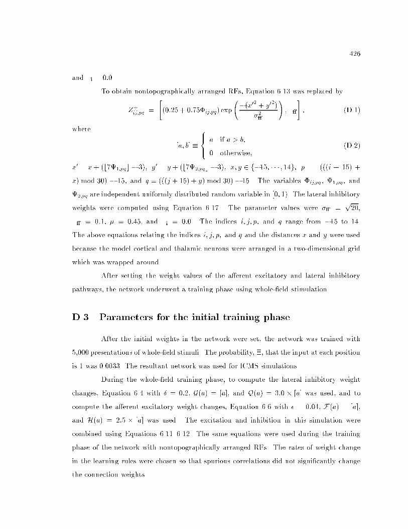
426and �i = 0:0.To obtain nontopographically arranged RFs, Equation 6.13 was replaced byZ+ij;pq = "(0:25 + 0:75�ij;pq) exp �(x02 + y02)�2� ! ;��# ; (D.1)where [a; b] � 8><>: a if a > b;0 otherwise; (D.2)x0 = x+ (b71;pqc � 3), y0 = y + (b72;pqc � 3), x; y 2 f�15; � � � ; 14g, p = (((i + 15) +x) mod 30) � 15, and q = (((j + 15) + y) mod 30)� 15. The variables �ij;pq, 1;pq, and2;pq are independent uniformly distributed random variable in [0; 1). The lateral inhibitoryweights were computed using Equation 6.17. The parameter values were �� = p20,�� = 0:1, � = 0:45, and �i = 0:0. The indices i; j; p; and q range from �15 to 14.The above equations relating the indices i; j; p; and q and the distances x and y were usedbecause the model cortical and thalamic neurons were arranged in a two-dimensional gridwhich was wrapped around.After setting the weight values of the a�erent excitatory and lateral inhibitorypathways, the network underwent a training phase using whole-�eld stimulation.D.3 Parameters for the initial training phaseAfter the initial weights in the network were set, the network was trained with5,000 presentations of whole-�eld stimuli. The probability, �, that the input at each positionis 1 was 0.0033. The resultant network was used for ICMS simulations.During the whole-�eld training phase, to compute the lateral inhibitory weightchanges, Equation 6.4 with � = 0:2, G(a) = [a], and Q(a) = 3:0 � [a] was used, and tocompute the a�erent excitatory weight changes, Equation 6.6 with � = 0:04, F(a) = [a],and H(a) = 2:5 � [a] was used. The excitation and inhibition in this simulation werecombined using Equations 6.11{6.12. The same equations were used during the trainingphase of the network with nontopographically arranged RFs. The rates of weight changein the learning rules were chosen so that spurious correlations did not signi�cantly changethe connection weights.

427D.4 Parameters for ICMS simulationsThe network obtained after the initial training phase (Section D.3) was used forICMS simulations.D.4.1 ICMS simulations in Section 6.3.1This simulation was performed on the network with topographically arranged RFs.The lateral inhibitory weight changes were governed by Equation 6.5 with � = 0:2,G(a) = [a], and Q(a) = 3:0 � [a], and a�erent excitatory weights changed according toEquation 6.7 with � = 0:04, F (a) = [a], and H(a) = 2:5� [a].The model ICMS was simulated using Equations 6.1{6.3 in Section 6.2.2 with(p0; q0) = (0; 0), (i0; j0) = (0; 0), '0 = 0:04, �1 = 10, �1 = 0:02, '1 = 0:37, �2 = 16:67,�3 = 50, �2 = 0:0037, '2 = 0:0686, �4 = 100, and �5 = 12:5. The excitationand inhibition during ICMS were combined using Equations 6.9{6.10. Model ICMS waspresented 500 times. To determine the temporal e�ects of ICMS the network was trainedwith an additional 500 presentations of ICMS.D.4.2 ICMS simulations in Section 6.3.2In all the simulations in this section, ICMS was presented 500 times. To determinethe role of a�erent excitatory synaptic plasticity in producing RF changes after ICMS,lateral inhibitory synaptic plasticity was disabled. To analyze the e�ects produced by lateralinhibitory synaptic plasticity rule, a�erent excitatory synaptic plasticity was disabled. Inthese two simulations, other parameters were the same as in Section 6.3.1 (see the previoussubsection).To determine the e�ects of the strength and distribution of direct excitation tomodel cortical neurons and excitation to a�erent excitatory synaptic terminals becauseof ICMS, the parameters in Equation 6.1 and Equation 6.2 were varied. The values ofparameters in Equation 6.1 were changed as follows. The value of '0 was independentlychanged from 0.04 to 80, and the value of '0 and �1 were simultaneously changed from0.04 to 80 and 10 to 100, respectively. The other parameter values were the same as in

428Section 6.3.1 (see the previous subsection).The values of parameters in Equation 6.2 were changed independently. The otherparameter values were the same as in Section 6.3.1 (see the previous subsection). The valueof �1 was changed from 0.02 to 0.04, '1 was changed from 0.37 to 0.555, �2 was changedfrom 16.67 to 33.34, and �3 was changed from 50 to 100.To analyze the e�ects of the strength and distribution of excitation to lateralinhibitory pathways induced by ICMS, the parameters in Equation 6.3 were independentlyvaried. The other parameter values were the same as in Section 6.3.1 (see the previoussubsection). The value of �2 was changed from 0.0037 to 0.0074, '2 was changed from0.0686 to 0.1372, �4 was changed from 100 to 200, and �5 was changed from 12.5 to 25.D.4.3 ICMS simulations in Section 6.3.3This simulation was performed on the network obtained after an initial trainingphase (Section D.3) on a network with nontopographically arranged RFs (Section D.2).The values for the parameters in Equations 6.1{6.3 were the same as those in Section 6.3.1.The ICMS was presented 500 times.D.5 Parameters for peripheral stimulation simulationsThe network obtained after the initial training phase (Section D.3) was usedfor ICMS simulations. During peripheral stimulation only lateral inhibitory learning wasenabled. To compute the lateral inhibitory weight changes, Equation 6.4 with � = 0:2,G(a) = [a], and Q(a) = 3:0� [a] was used. These parameter values are the same as in thelateral inhibitory synaptic plasticity rule during the initial training phase (Section D.3).The total excitation and inhibition to the model cortical neurons were computed usingEquations 6.11{6.12.To simulate strong localized peripheral stimulation a truncated Gaussianconvolution kernel K was centered at Layer 1 location (0; 0). To simulate weak localizedperipheral stimulation, K was scaled by a multiplicative factor of 0.15. The peripheral

429stimulation was presented 1000 times. The kernel K wasK = 266664 0:55 0:74 0:550:74 1:00 0:740:55 0:74 0:55 377775 :D.6 Parameters for RF measurementsThe RF was mapped using single-point stimulation, blurred with the kernel K,at all input positions (i; j). The activation of model cortical neurons was scaled relative tothe maximal activation of model cortical neurons in response to the RF test input, K, overall the input locations. The RF of a Layer 2 neuron (p; q) was de�ned as the collection ofpositions (i; j) at which the test input caused the scaled activation of model cortical neuronsto exceed a threshold � = 0:01.

430Bibliography[1] Abraham, W.C. & Goddard, G.V. (1983) Asymmetric relationships betweenhomosynaptic long-term potentiation and heterosynaptic long-term depression. Nature,305, 717{719.[2] Ahmed, B.A., Anderson, J.C., Douglas, R.J., Martin, K.A.C., & Nelson, J.C. (1994)Polyneuronal innervation of spiny stellate neurons in cat visual cortex. The Journal ofComparative Neurology , 341, 39{49.[3] Andersen, P., Sundberg, S.H., Sveen, O., & Wigstr�om, H. (1977) Speci�c long-lastingpotentiation of synaptic transmission in hippocampal slices. Nature, 266, 736{737.[4] Artola, A., Br�ocher, S., & Singer, W. (1990) Di�erent voltage-dependent threshold forinducing long-term depression and long-term potentiation in slices of rat visual cortex.Nature, 347, 69{72.[5] Artola, A. & Singer, W. (1987) Long-term potentiation and NMDA receptors in ratvisual cortex. Nature, 330, 649{652.[6] Atick, J. & Redlich, A. (1990) Toward a theory of early visual processing. NeuralComputation , 2, 308{320.[7] Badcock, D.R. & Westheimer, G. (1985) Spatial location and hyperacuity: Thecenter-surround localization function has two substrates. Vision Research, 25, 1259{1269.[8] Baloch, A.A. & Grossberg, S. (1997) A neural model of high-level motion processing:Line motion and formotion dynamics. Vision Research, 37 (21), 3037{3059.

431[9] Barlow, H.B., Blakemore, C., & Pettigrew, J.D. (1967) The neural mechanism ofbinocular depth discrimination. Journal of Physiology , 193, 327{342.[10] Barrionuevo, G. & Brown, T.H. (1983) Associative long-term potentiation inhippocampal slices. Proceedings of the National Academy of Sciences of the USA, 80,7347{7351.[11] Bear, M.F., Cooper, L.N., & Ebner, F.F. (1987) The physiological basis of a theory forsynapse modi�cation. Science, 237, 42{48.[12] Bear, M.F., Kleinschmidt, A., Gu, Q., & Singer, W. (1990) Disruption of experience-dependent synaptic modi�cations in striate cortex by infusion of an NMDA receptorantagonist. The Journal of Neuroscience, 10(3), 909{925.[13] Bear, M.F., Press, W.A., & Connors, B.W. (1992) Long-term potentiation in slicesof kitten visual cortex and the e�ects of NMDA receptor blockade. Journal ofNeurophysiology , 67(4), 841{851.[14] Bednar, J.A. & Miikkulainen, R. (1997) A neural network model of visual tiltaftere�ect. In Proceedings of the 19th Annual Conference of the Cognitive ScienceSociety , 37{42. Hillsdale, NJ: Erlbaum.[15] Benevento, L.A., Creutzfeldt, O.D., & Kuhnt, U. (1972) Signi�cance of intracorticalinhibition in the visual cortex. Nature, 238, 124{126.[16] Bienenstock, E.L., Cooper, L.N., & Munro, P.W. (1982) Theory for the developmentof neuron selectivity: Orientation speci�city and binocular interaction in visual cortex.The Journal of Neuroscience, 2, 32{48.[17] Blake, R. (1989) A neural theory of binocular rivalry. Psychological Review , 96, 145{167.[18] Blake, R., Fox, R., & McIntyre, C. (1971) Stochastic properties of stabilized-imagedbinocular rivalry alternations. Journal of Experimental Psychology , 88, 327{332.

432[19] Blake, R. & O'Shea, R.P. (1988) \Abnormal fusion" of stereopsis and binocular rivalry.Psychological Review , 95, 151{154.[20] Blake, R., Yang, Y., & Wilson, H.R. (1991) On the coexistence of stereopsis andbinocular rivalry. Vision Research, 31, 1191{1203.[21] Blakemore, C., Carpenter, R.H.S., & Georgeson, M.A. (1970) Lateral inhibitionbetween orientation detectors in the human visual system. Nature, 228, 37{39.[22] Blakemore, C., Fiorentini, A., & Ma�ei, L. (1972) A second neural mechanism ofbinocular depth discrimination. Journal of Physiology , 226, 725{749.[23] Blakemore, C. & Nachmias, J. (1971) The orientation speci�city of two visualafter-e�ects. Journal of Physiology , 213, 157{174.[24] Blakemore, C. & Tobin, E.A. (1972) Lateral inhibition between orientation detectorsin the cat's visual cortex. Experimental Brain Research, 15, 439{440.[25] Blakemore, C. & Van Sluyters, R.C. (1974) Reversal of the physiological e�ects ofmonocular deprivation in kittens: Further evidence for a sensitive period. Journal ofPhysiology , 237, 195{216.[26] Blakemore, C. & Van Sluyters, R.C. (1975) Innate and environmental factors in thedevelopment of the kitten's visual cortex. Journal of Physiology , 248, 663{716.[27] Blasdel, G.G. (1992a) Di�erential imaging of ocular dominance and orientationselectivity in monkey striate cortex. The Journal of Neuroscience, 12, 3115{3138.[28] Blasdel, G.G. (1992b) Orientation selectivity, preference and continuity in monkeystriate cortex. The Journal of Neuroscience, 12, 3139{3161.[29] Blasdel, G.G., Lund, J.S., & Fitzpatrick, D. (1985) Intrinsic connections of macaquestriate cortex: Axonal projections of cells outside lamina 4C. The Journal ofNeuroscience, 5, 3350{3369.

433[30] Blasdel, G.G., Obermayer, K., & Kiorpes, L. (1995) Organization of ocular dominanceand orientation columns in the striate cortex of neonatal macaque monkeys. VisualNeuroscience, 12, 589{603.[31] Blasdel, G.G. & Salama, G. (1986) Voltage sensitive dyes reveal a modular organizationin monkey striate cortex. Nature, 321, 579{585.[32] Bonds, A.B. & DeBruyn, E.J. (1985) Inhibition and spatial selectivity in the visualcortex: The cooperative neuronal network revisited. In Models of the Visual Cortex ,D. Rose & V.G. Dobson (eds.), 292{299. New York: John Wiley & Sons.[33] Bonhoe�er, T. & Grinvald, A. (1991) Iso-orientation domains in cat visual cortex arearranged in pinwheel-like patterns. Nature, 353, 429{431.[34] Bosking, W.H., Zhang, Y, Scho�eld, B., & Fitzpatrick, D. (1997) Orientation selectivityand the arrangement of horizontal connections in tree shrew striate cortex. The Journalof Neuroscience, 17(6), 2112{2127.[35] Breese, B.B. (1899) On inhibition. Psychological Review , 3(11).[36] Breese, B.B. (1909) Binocular rivalry. Psychological Review , 16, 410{415.[37] Brown, T.H. & Chattarji, S. (1995) Hebbian synaptic plasticity. In The Handbook ofBrain Theory and Neural Networks , M.A. Arbib (ed.), 454{459. Cambridge, MA: MITPress.[38] Brown, T.H., Kairiss, E.W., & Keenan, C.L. (1990) Hebbian synapses: Biophysicalmechanisms and algorithms. Annual Review of Neuroscience, 13, 475{511.[39] Buisseret, P., Gary-Bobo, E., & Imbert, M. (1982) Plasticity in the kitten's visualcortex: E�ects of the suppression of visual experience upon the orientational propertiesof visual cortical cells. Developmental Brain Research, 4, 417{426.[40] Butler, T. & Westheimer, G. (1978) Interference with stereoscopic acuity: Spatial,temporal, and disparity tuning. Vision Research, 18, 1387{1392.

434[41] Callaway, E.M. & Katz, L.C. (1990) Emergence and re�nement of clustered horizontalconnections in cat striate cortex. The Journal of Neuroscience, 10, 1134{1153.[42] Campbell, F.W. & Howell, E.R. (1972) Monocular alternation: A method for theinvestigation of pattern vision. Journal of Physiology , 225, 19{21.[43] Carew, T.J., Hawkins, R.D., Abrams, T.W., & Kandel, E.R. (1984) A test of Hebb'spostulate at identi�ed synapses which mediate classical conditioning in Aplysia. TheJournal of Neuroscience, 4, 1217{1224.[44] Carpenter, G. & Grossberg, S. (1987) A massively parallel architecture for aself-organizing neural pattern recognition machine. Computer Vision, Graphics, andImage Processing , 37, 54{115.[45] Chapman, B. & Stone, L.S. (1996) Turning a blind eye to cortical receptive �elds.Neuron, 16, 9{12.[46] Chapman, B., Stryker, M.P., & Bonhoe�er, T. (1996) Development of orientationpreference maps in ferret primary visual cortex. The Journal of Neuroscience, 16,6443{6453.[47] Chino, Y.M., Kaas, J.H., Smith III, E.L., Langston, A.L., & Cheng, H. (1992) Rapidreorganization of cortical maps in adult cats following restricted dea�erentation inretina. Vision Research, 32(5), 789{796.[48] Chino, Y., Smith, E., Hatta, S., & Cheng, H. (1997) Postnatal development ofbinocular disparity sensitivity in neurons of the primate visual cortex. The Journalof Neuroscience, 17, 1{12.[49] Clothiaux, E.E., Cooper, L.N., & Bear, M.F. (1991) Synaptic plasticity in visualcortex: Comparison of theory with experiment. Journal of Physiology , 66, 1785{1804.[50] Cohen, M.A. & Grossberg, S. (1983) Absolute stability of global pattern formationand parallel memory storage by competitive neural networks. IEEE Transactions onSystems, Man, and Cybernetics , 13(5), 815{826.

435[51] Crepel, J., Hemart, N., Jaillard, D., & Daniel, H. (1995) Long-term depression in thecerebellum. In The Handbook of Brain Theory and Neural Networks , M.A. Arbib (ed.),560{563. Cambridge, MA: MIT Press.[52] Crist, R.E., Kapadia, M.K., Westheimer, G., & Gilbert, C.D. (1997) Perceptuallearning of spatial localization: Speci�city for orientation, position, and context.Journal of Neurophysiology , 78(6), 2889{2894.[53] Cynader, M. (1983) Prolonged sensitivity to monocular deprivation in dark-reared cats:E�ects of age and visual exposure. Developmental Brain Research, 8, 155{164.[54] Dalva, M.B. & Katz, L.C. (1994) Rearrangements of synaptic connections in visualcortex revealed by laser photostimulation. Science, 265, 255{258.[55] Darian-Smith, C. & Gilbert, C.D. (1994) Axonal sprouting accompanies functionalreorganization in adult cat striate cortex. Nature, 368, 737{740.[56] Darian-Smith, C. & Gilbert, C.D. (1995) Topographic reorganization in the striatecortex of the adult cat and monkey is cortically mediated. The Journal of Neuroscience,15(3), 1631{1647.[57] Das, A. (1997) Plasticity in adult sensory cortex: A review. Network: Computation inNeural Systems , 8, R33{R76.[58] Das, A. & Gilbert, C.D. (1995a) Long-range horizontal connections and their rolein cortical reorganization revealed by optical recording of cat primary visual cortex.Nature, 375, 780{784.[59] Das, A. & Gilbert, C.D. (1995b) Receptive �eld expansion in adult visual cortexis linked to dynamic changes in strength of cortical connections. Journal ofNeurophysiology , 74(2), 779{792.[60] DeAngelis, G.C., Anzai, A., Ohzawa, I., & Freeman, R.D. (1992) Organizationof suppression in receptive �elds of neurons in cat visual cortex. Journal ofNeurophysiology , 68(1), 144{163.

436[61] DeAngelis, G.C., Anzai, A., Ohzawa, I., & Freeman, R.D. (1995) Receptive �eldstructure in the visual cortex: Does selective stimulation induce plasticity? Proceedingsof the National Academy of Sciences of the USA, 92, 9682{9686.[62] DeAngelis, G.C., Ohzawa, I., Anzai, A., & Freeman, R.D. (1994) Does an arti�cialscotoma induce plasticity of receptive �eld structure for neurons in the visual cortex?Investigative Ophthalmology & Visual Science, 35(4), 1468.[63] DeAngelis, G.C., Ohzawa, I., & Freeman, R.D. (1991) Depth is encoded in the visualcortex by a specialized receptive �eld structure. Nature, 352, 156{159.[64] Debanne, D., G�ahwiler, B.H., & Thompson, S.M. (1997) Bidirectional associativeplasticity of unitary CA3-CA1 EPSPs in the rat hippocampus in vitro. Journal ofNeurophysiology , 77, 2851{2855.[65] O'Dell, C. & Boothe, R.G. (1997) The development of stereoacuity in infant rhesusmonkeys. Vision Research, 37, 2675{2684.[66] DeSieno, D. (1988) Adding a conscience to competitive learning. In IEEE 1stInternational Conference on Neural Networks, Volume 1, M. Caudill & C. Butler (eds.),117{124. San Diego: IEEE.[67] Dews, P.B. & Wiesel, T.N. (1970) Consequences of monocular deprivation on visualbehavior in kittens. Journal of Physiology , 206, 437{455.[68] Douglas, R.J. & Martin, K.A.C. (1991) A functional microcircuit for cat visual cortex.Journal of Physiology , 440, 735{769.[69] Dudek, S.M. & Bear, M.F. (1992) Homosynaptic long-term depression in area CA1 ofhippocampus and the e�ects on NMDA receptor blockade. Proceedings of the NationalAcademy of Sciences of the USA, 89, 4363{4367.[70] Einstein, G., Davis, T.L., & Sterling, P. (1987) Pattern of lateral geniculate synapseson neuron somata in layer IV of the cat striate cortex. The Journal of ComparativeNeurology , 260, 76{86.

437[71] Engel, A.K., K�onig, P., & Singer, W. (1991) Direct physiological evidence for scenesegmentation by temporal coding. Proceedings of the National Academy of Sciences ofthe USA, 88, 9136{9140.[72] Erwin, E., Obermayer, K., & Schulten, K. (1995) Models of orientation and oculardominance columns in the visual cortex: A critical comparison. Neural Computation,7, 425{468.[73] Fahle, M. (1997) Speci�city of learning curvature, orientation, and vernierdiscriminations. Vision Research, 37(14), 1885{1895.[74] Fahle, M. & Edelman, S. (1993) Long-term learning in vernier acuity: E�ects ofstimulus orientation, range and of feedback. Vision Research, 33, 397{412.[75] Fahle, M., Edelman, S., & Poggio, T. (1995) Fast perceptual learning in hyperacuity.Vision Research, 35, 3003{3013.[76] Felleman, D.J. & Van Essen, D.C. (1991) Distributed hierarchical processing in theprimate cerebral cortex. Cerebral Cortex , 1, 1{47.[77] Favorov, O.V. & Kelly, D.G. (1994a) Minicolumnar organization within somatosensorycortical segregates: I. Development of a�erent connections. Cerebral Cortex , 4(4), 408{427.[78] Favorov, O.V. & Kelly, D.G. (1994b) Minicolumnar organization within somatosensorycortical segregates: II. Emergent functional properties. Cerebral Cortex , 4(4), 428{442.[79] Favorov, O.V. & Kelly, D.G. (1996) Local receptive �eld diversity within corticalneuronal populations. In Somesthesis and the Neurobiology of the SomatosensoryCortex , O. Franz�en, R. Johansson, & L. Terenius (eds.), 395{408. Basel, Switzerland:Birkh�auser Verlag.[80] Ferster, D.L. (1986) Orientation selectivity of synaptic potentials in neurons of catprimary visual cortex. The Journal of Neuroscience, 6(5), 1284{1301.

438[81] Ferster, D.L. (1989) The synaptic inputs to simple cells of the cat visual cortex. InProceedings of the Retina Research Foundation, Volume 2: Neural Mechanisms ofVisual Perception, D.M. Lam & C.D. Gilbert (eds.), 63{85. Texas: Portfolio.[82] Fiorentini, A. & Berardi, N. (1980) Perceptual learning is speci�c for orientation andspatial frequency. Nature, 287, 43{44.[83] Fitzpatrick, D., Lund, J.S., & Blasdel, G.G. (1985) Intrinsic connections of macaquestriate cortex: A�erent and e�erent connections of lamina 4C. The Journal ofNeuroscience, 5, 3329{3349.[84] Fox, K. & Daw, N.W. (1993) Do NMDA receptors have a critical function in visualcortical plasticity? Trends in Neurosciences , 16(3), 116{122.[85] Freeman, R.D., Mallach, R., & Hartley, S. (1981) Responsitivity of normal kitten striatecortex deteriorates after brief binocular deprivation. Journal of Neurophysiology , 45,1074{1084.[86] Freeman, R.D. & Olson, C. (1982) Brief periods of monocular deprivation in kittens:E�ects of delay prior to physiological study. Journal of Neurophysiology , 47, 139{150.[87] Fr�egnac, Y., Burke, J.P., Smith, D., & Friedlander, M.J. (1994) Temporal covarianceof pre- and postsynaptic activity regulates functional connectivity in the visual cortex.Journal of Neurophysiology, 71(4), 1403{1421.[88] Fr�egnac, Y. & Imbert, M. (1978) Early development of visual cortical cells in normaland dark-reared kittens: Relationship between orientation selectivity and oculardominance. Journal of Physiology , 278, 27{44.[89] Fr�egnac, Y. & Imbert, M. (1984) Development of neuronal selectivity in primary visualcortex of cat. Physiological Review , 64, 325{434.[90] Fr�egnac, Y., Shulz, D., Thorpe, S., & Bienenstock, E. (1988) A cellular analogue ofvisual cortical plasticity. Nature, 333, 367{370.

439[91] Frisby, J.P. & Pollard, S.B. (1991) Computational issues in solving the stereocorrespondence problem. In Computational Models of Visual Processing , M.S. Landy &J.A. Movshon (eds.), 331{358. Cambridge, MA: MIT Press.[92] Garraghty, P.E., Pons, T.P., Sur, M., & Kaas, J.H. (1989) The arbors of axonsterminating in middle cortical layers of somatosensory area 3b in owl monkeys.Somatosensory and Motor Research, 6, 401{411.[93] Garraghty, P.E. & Sur, M. (1990) Morphology of single intracellularly stained axonsterminating in area 3b of macaque monkeys. The Journal of Comparative Neurology ,294, 583{593.[94] Gil, Z. & Amitai, Y. (1996) Spatial integration and cortical dynamics. The Journal ofNeuroscience, 16(20), 6567{6578.[95] Gilbert, C.D. (1996) Plasticity in visual perception and physiology. Current Opinionin Neurobiology , 6(2), 269{274.[96] Gilbert, C.D. (1998) Adult cortical dynamics. Physiological Review , 78(2), 467{485.[97] Gilbert, C.D., Das, A., Ito, M., Kapadia, M., & Westheimer, G. (1996) Spatialintegration and cortical dynamics. Proceedings of the National Academy of Sciencesof the USA, 93, 615{622.[98] Gilbert, C.D., Hirsch, J.A., & Wiesel, T.N. (1990) Lateral interactions in visual cortex.In Cold Spring Harbor Symposia on Quantitative Biology , 55, 663{677. Cold SpringHarbor, NY: Cold Spring Harbor Laboratory Press.[99] Gilbert, C.D. & Wiesel, T.N. (1979) Morphology and intracortical projections offunctionally characterised neurones in the cat visual cortex. Nature, 280, 120{125.[100] Gilbert, C.D. & Wiesel, T.N. (1983) Clustered intrinsic connections in cat visualcortex. The Journal of Neuroscience, 3(5), 1116{1133.

440[101] Gilbert, C.D. & Wiesel, T.N. (1989) Columnar speci�city of intrinsic horizontal andcorticocortical connections in cat visual cortex. The Journal of Neuroscience, 9(7),2432{2442.[102] Gilbert, C.D. & Wiesel, T.N. (1990) The in uence of contextual stimuli on theorientation selectivity of cells in primary visual cortex of the cat. Vision Research,30, 11, 1689{1701.[103] Gilchrist, A.L. (1994) Lightness, Brightness, and Transparency . Hillsdale, NJ:Erlbaum.[104] Goda, Y. & Stevens, C.F. (1996) Long-term depression properties in a simple system.Neuron, 16, 103{111.[105] Gove, A., Grossberg, S., & Mingolla, E. (1995) Brightness perception, illusorycontours, and corticogeniculate feedback. Visual Neuroscience, 12, 1027{1052.[106] Grajski, K.A. & Merzenich, M.M. (1990) Hebb-type dynamics is su�cient to accountfor the inverse magni�cation rule in cortical somatotopy. Neural Computation, 2, 71{84.[107] Gray, C.M. & Singer, W. (1989) Stimulus-speci�c neuronal oscillations in orientationcolumns of cat visual cortex. Proceedings of the National Academy of Sciences of theUSA, 86, 1698{1702.[108] Gray, C.M., K�onig, P., Engel, A.K., & Singer, W. (1989) Oscillatory responses incat visual cortex exhibit inter-column synchronization which re ects global stimulusproperties. Nature, 338, 334{337.[109] Grossberg, S. (1972) Neural expectation: Cerebellar and retinal analogs of cells �redby learnable or unlearned pattern classes. Kybernetik , 10, 49{57.[110] Grossberg, S. (1976a) On the development of feature detectors in the visual cortexwith applications to learning and reaction-di�usion systems. Biological Cybernetics,21, 145{159.

441[111] Grossberg, S. (1976b) Adaptive pattern classi�cation and universal recoding:I. Parallel development and coding of neural feature detectors. Biological Cybernetics ,23, 121{134.[112] Grossberg, S. (1976c) Adaptive pattern classi�cation and universal recoding:II. Feedback, expectation, olfaction, and illusions. Biological Cybernetics , 23, 187{202.[113] Grossberg, S. (1978) A theory of human memory: Self-organization and performanceof sensory-motor codes, maps, and plans. In Progress in Theoretical Biology, Volume 5 ,R. Rosen & F. Snell (eds.). New York: Academic Press.[114] Grossberg, S. (1980) How does brain build a cognitive code? Psychological Review ,89, 529{572.[115] Grossberg, S. (1982) Studies of Mind and Brain: Neural Principles of Learning,Perception, Development, Cognition, and Motor Control . Boston, MA: Reidel Press.[116] Grossberg, S. (1985) The adaptive self-organization of serial order in behavior:Speech, language, and motor control. In Pattern Recognition by Humans and Machines,Volume 1: Speech Perception, E.C. Schwab & H.C. Nusbaum (eds.). New York:Academic Press.[117] Grossberg, S. (1987) Cortical dynamics of three-dimensional form, color andbrightness perception: 2. Binocular rivalry. Perception & Psychophysics , 41, 117{158.[118] Grossberg, S., Boardman, I., & Cohen, M.A. (1997a) Neural dynamics of variable-ratespeech categorization. Journal of Experimental Psychology: Human Perception andPerformance, 23, 418{503.[119] Grossberg, S. & Marshall, J.A. (1989) Stereo boundary fusion by cortical complexcells: A system of maps, �lters, and feedback networks for multiplexing distributeddata. Neural Networks , 2, 29{51.[120] Grossberg, S. & Merrill, J.W.L. (1996)The hippocampus and cerebellum in adaptivelytimed learning, recognition, and movement. Journal of Cognitive Neuroscience, 8, 257{277.

442[121] Grossberg, S. & Mingolla, E. (1985a) Neural dynamics of form perception: Boundarycompletion, illusory �gures, and neon color spreading. Psychological Review , 92, 173{211.[122] Grossberg, S. & Mingolla, E. (1985b) Neural dynamics of form perception: Textures,boundaries, and emergent and segmentations. Perception and Psychophysics , 38, 141{171.[123] Grossberg, S., Mingolla, E., & Ross, W.D. (1994) A neural theory of attentivevisual search: Interactions of boundary, surface, spatial, and object representations.Psychological Review , 101(3), 470{489.[124] Grossberg, S., Mingolla, E., & Ross, W.D. (1997b) Visual brain and visual perception:How does the cortex do perceptual grouping? Trends in Neurosciences , 20(3), 106{111.[125] Grossberg, S. & Olson, S.J. (1994) Rules for the cortical map of ocular dominanceand orientation columns. Neural Networks , 7, 883{894.[126] Grossberg, S. & Rudd, M.E. (1992) Cortical dynamics of visual motion perception:Short-range and long-range apparent motion. Psychological Review , 99(1), 78{121.[127] Grunewald, A. & Grossberg, S. (1997) Self-organization of binocular disparitytuning by reciprocal corticogeniculate interactions. In press, Journal of CognitiveNeuroscience.[128] Hammond, P., Mouat, G.S., & Smith, A.T. (1986) Motion after-e�ects in cat striatecortex elicited by moving textures. Vision Research, 26(7), 1055{1060.[129] Hammond, P., Pomfrett, C.J.D., & Ahmed, B. (1989) Neural motion after-e�ects inthe cat's striate cortex: Orientation selectivity. Vision Research, 29(12), 1671{1683.[130] Held, R., Birch, E, & Gwiazda, J. (1980) Stereoacuity of human infants. Proceedingsof the National Academy of Sciences of the USA, 77, 5572{5574.

443[131] Hendry, S.H.C., Fuchs, J., deBlas, A.J., & Jones, E.G. (1990) Distribution andplasticity of immunocytochemically localized GABAA receptors in adult monkey visualcortex. The Journal of Neuroscience, 10, 2438{2450.[132] Herzog, M.H. & Fahle, M. (1995) A recurrent model for learning a hyperacuity task.Perception, 24, S84.[133] Hess, G. & Donoghue, J.P. (1994) The in uence of prior synaptic activity on theinduction of long-term potentiation. Journal of Neurophysiology , 71(6), 2543{2547.[134] Heynen, A.J., Abraham, W.C., & Bear, M.F. (1996) Bidirectional modi�cation ofCA1 synapses in the adult hippocampus in vivo. Nature, 381, 163{166.[135] Hirsch, J. & Gilbert, C.D. (1991) Synaptic physiology of horizontal connections in thecat's visual cortex. The Journal of Neuroscience, 11, 1800{1809.[136] Hirsch, J.A. & Gilbert, C.D. (1993) Long-term changes in synaptic strength alongspeci�c intrinsic pathways in the cat visual cortex. Journal of Physiology , 461, 247{262.[137] Hodgkin, A.L. (1964) The Conduction of the Nervous Impulse. Liverpool, England:Liverpool University Press.[138] Huang, Y.Y., Colino, A., Selig, D.K., & Malenka, R.C. (1992) The in uence of priorsynaptic activity on the induction of long-term potentiation. Science, 225, 730{733.[139] Hubbard, R.S. & Marshall, J.A. (1994) Self-organizing neural network model of thevisual inertia phenomenon in motion perception. Technical Report 94{001, Universityof North Carolina at Chapel Hill, Department of Computer Science, 26 pp.[140] Hubel, D.H. & Wiesel, T.N. (1962) Receptive �elds, binocular interaction, andfunctional architecture in the cat's visual cortex. Journal of Physiology , 160, 106{154.[141] Hubel, D.H. & Wiesel, T.N. (1963) Receptive �elds of cells in striate cortex of veryyoung, visually inexperienced kittens. Journal of Neurophysiology , 26, 994{1002.

444[142] Hubel, D.H. & Wiesel, T.N. (1965) Binocular interaction in striate cortex of kittenreared with arti�cial squint. Journal of Neurophysiology , 28, 1041{1059.[143] Hubel, D.H. & Wiesel, T.N. (1970) The period of susceptibility to the physiologicale�ects of unilateral eye closure in kittens. Journal of Physiology, 206, 419{436.[144] Hubel, D.H. & Wiesel, T.N. (1972) Laminar and columnar distribution ofgeniculo-cortical �bers in the macaque monkey. The Journal of Comparative Neurology ,146, 421{450.[145] Hubel, D.H., Wiesel, T.N., & LeVay, S. (1977) Plasticity of ocular dominance columnsin monkey striate cortex. Philosophical Transactions of the Royal Society (London),278, 377{409.[146] H�ubener, M, Shoham, D., Grinvald, A., & Bonhoe�er, T. (1997) Spatial relationshipsamong three columnar systems in cat area 17. The Journal of Neuroscience, 17(23),9270{9284.[147] Humphrey, A.L., Sur, M., Ulrich, D.J., & Sherman, S.M. (1985) Receptive �elds,binocular interaction, and functional architecture in the cat's visual cortex.The Journalof Comparative Neurology , 233, 159{189.[148] Intrator, N. (1992) Feature extraction using an unsupervised neural network. NeuralComputation , 4, 98{107.[149] Intrator, N. & Cooper, L.N. (1992) Objective function formulation of the BCMtheory of visual cortical plasticity: Statistical connections, stability conditions. NeuralNetworks , 5, 3{17.[150] Intrator, N. & Cooper, L.N. (1995) BCM theory of visual cortical plasticity. InThe Handbook of Brain Theory and Neural Networks , M.A. Arbib (ed.), 153{157.Cambridge, MA: MIT Press.[151] Iwamura, Y., Tanaka, M., Sakamoto, M., & Hikosaka, O. (1983) Functionalsubdivisions representing di�erent �nger regions in area 3 of the �rst somatosensorycortex of conscious monkey. Experimental Brain Research, 51, 315{326.

445[152] Jenkins, W.M., Merzenich, M.M., Ochs, M.T., Allard, T., & Gu��c-Robles, E. (1990)Functional reorganization of primary somatosensory cortex in adult owl monkey afterbehaviorally controlled tactile stimulation. Journal of Neurophysiology, 63(1), 82{104.[153] Johansson, G. (1950) Con�gurations in Event Perception. Stockholm, Sweden:Almqvist & Wiksell.[154] Juliano, S.L. & Whitsel, B.L. (1987) A combined 2-deoxyglucose andneurophysiological study of primate somatosensory cortex. The Journal of ComparativeNeurology , 263, 514{525.[155] Kang, R., Herman, D., MacGillis, M., & Zarzecki, P. (1985) Convergence ofsensory inputs in somatosensory cortex: Interactions from separate a�erent sources.Experimental Brain Research, 57, 271{278.[156] Kalarickal, G.J. & Marshall, J.A. (1996a) Dynamic receptive �elds in visual cortex:Adaptive neural model and predictions. Investigative Ophthalmology & Visual Science,37(3), 483.[157] Kalarickal, G.J. & Marshall, J.A. (1996b) Dynamic cortical receptive �eld changes:Neuronal adaptation or connection plasticity? Society for Neuroscience Abstracts , 22,1613.[158] Kalarickal, G.J. & Marshall, J.A. (1996c) Synaptic plasticity: Comparison of EXINand BCM learning rules. Journal of Mathematical Psychology , 40(4), 355.[159] Kalarickal, G.J. & Marshall, J.A. (1997a) The role of feedforward excitatory andlateral inhibitory learning in visual classical rearing. Investigative Ophthalmology &Visual Science, 38(4), 360.[160] Kalarickal, G.J. & Marshall, J.A. (1997b) Receptive �eld dynamics in visual cortex:Models based on synaptic plasticity and neuronal adaptation. Technical Report 97-029,Department of Computer Science, University of North Carolina at Chapel Hill.[161] Kalarickal, G.J. & Marshall, J.A. (1998a)Modeling temporal and stochastic propertiesof binocular rivalry. Investigative Ophthalmology & Visual Science, 39(4), 862.

446[162] Kalarickal, G.J. & Marshall, J.A. (1998b) Modeling dynamic receptive �eld changesproduced by intracortical microstimulation. In press, Computational Neuroscience:Trends in Research, 1998, J.M. Bower (ed.).[163] Kano, M., Lino, K., & Kano, M. (1991) Functional reorganization of adult catsomatosensory cortex is dependent on NMDA receptors. NeuroReport , 2, 77{80.[164] Kano, M., Rexhausen, U., Dreessen, J., & Konnerth, A. (1996) Synaptic excitationproduces a long-lasting rebound potentiation of inhibitory synaptic signals in cerebellarPurkinje cells. Nature, 356, 601{604.[165] Kapadia, M.K., Gilbert, C.D., & Westheimer, G. (1994) A quantitative measure forshort-term cortical plasticity in human vision. The Journal of Neuroscience, 14(1),451{457.[166] Kapadia, M.K., Ito, M., Gilbert, C.D., & Westheimer, G. (1995) Improvement invisual sensitivity by changes in local context: Parallel studies in human observers andin V1 of alert monkeys. Neuron, 15, 843{856.[167] Karni, A. & Sagi, D. (1991) Where practice makes perfect in texture discrimination:Evidence for primary visual cortex plasticity. Proceedings of the National Academy ofSciences of the USA, 88, 4966{4970.[168] Kasamatsu, T., Imamura, K., & Mataga, N. (1997) Abnormal response propertiesin APV-infused, otherwise normal visual cortex of adult cats. InvestigativeOphthalmology & Visual Science, 38(4), 106.[169] Kasamatsu, T., Imamura, K., Mataga, N., Hartveit, E., Heggelund, U., &Heggelund, P. (1998a) Roles of N-methyl-D-aspartate receptors in ocular dominanceplasticity in developing visual cortex: Re-evaluation. Neuroscience, 82(3), 687{700.[170] Kasamatsu, T., Kitano, M., Sutter, E.E., & Norcia, A.M. (1998b) Lack of lateralinhibitory interactions in visual cortex of monocularly deprived cats. Vision Research,38, 1{12.

447[171] Katz, L.C. & Callaway, E.M. (1992) Development of local circuits in mammalianvisual cortex. Annual Review of Neuroscience, 15, 31{56.[172] Kelso, S.R. & Brown, T.H. (1986) Di�erential conditioning of associative synapticenhancement in hippocampal brain slices. Science, 232, 85{87.[173] Kirkwood, A. & Bear, M.F. (1994) Homosynaptic long-term depression in the visualcortex. The Journal of Neuroscience, 14(5), 3404{3412.[174] Kirkwood, A., Dudek, S.M., Gold, J.T., Aizenman, C.D., & Bear, M.F. (1993)Common forms of synaptic plasticity in hippocampus and neocortex in vitro. Science,260, 1518{1521.[175] Kobayashi, K., Manabe, T., & Takahashi, T. (1996) Presynaptic long-term depressionat the hippocampal mossy �ber{CA3 synapse. Science, 273, 648{650.[176] Kohonen, T. (1987) Self-Organization and Associative Memory. New York:Springer-Verlag.[177] Kohonen, T. (1988) The \neural" phonetic typewriter. Computer , 21, 11-22.[178] K�onig, P., Engel, A., & Singer, W. (1995) Relation between oscillatory activity andlong-range synchronization in cat visual cortex. Proceedings of the National Academyof Sciences of the USA, 92, 290{294.[179] Land, E.H. (1986) Recent advances in retinex theory. Vision Research, 26, 7{21.[180] Lane, R.D., Killackey, H.P, & Rhoades, R.W. (1997) Blockade of GABAergicinhibition reveals reordered cortical somatotopic maps in rats that sustained neonatalforelimb removal. Journal of Neurophysiology , 77, 2723{2735.[181] Law, C.C. & Cooper, L.N. (1994) Formation of receptive �elds in realistic visualenvironments according to the BCM theory. Proceedings of the National Academy ofSciences of the USA, 91, 7797{7801.[182] Lehky, S.R. (1988) An astable multivibrator model of binocular rivalry. Perception,17, 215{228.

448[183] Lehky, S.R. & Blake, R. (1991) Organization of binocular pathways: Modeling anddata related to rivalry. Neural Computation, 3, 44{53.[184] Lehky, S.R. & Maunsell, J.H.R. (1996) No binocular rivalry in the LGN of alertmacaque monkeys. Vision Research, 36, 1225{1234.[185] Leopold, D.A. & Logothetis, N.K. (1996) Activity changes in early visual cortex re ectmonkeys' percepts during binocular rivalry. Nature, 379, 549{553.[186] LeVay, S., Wiesel, T.N., & Hubel, D.H. (1980) The development of ocular dominancecolumns in normal and visually deprived monkeys. The Journal of ComparativeNeurology , 191, 1{51.[187] Levelt, W.J.M. (1965) On Binocular Rivalry . Soesterberg, The Netherlands: Institutefor Perception RVO-TNO.[188] Levy, W.B. (1985) Associative changes at the synapse: LTP in the hippocampus.In Synaptic Modi�cation, Neuron Selectivity, and Nervous System Organization,W.B. Levy, J.A. Anderson, & S. Lehmkuhle (eds.), 5{33. Hillsdale, NJ: Erlbaum.[189] Levy, W.B. & Burger, B. (1987) Electrophysiological observations which help describean associative synaptic modi�cation rule. In IEEE 1st International Conference onNeural Networks, Volume 4, M. Caudill & C. Butler (eds.), 11{15. San Diego: IEEE.[190] Levy, W.B. & Desmond, N.L. (1985) The rules of elemental synaptic plasticity.In Synaptic Modi�cation, Neuron Selectivity, and Nervous System Organization,W.B. Levy, J.A. Anderson, & S. Lehmkuhle (eds.), 105{121. Hillsdale, NJ: Erlbaum.[191] Levy, W.B. & Steward, O. (1979) Synapses as associative memory elements in thehippocampal formation. Brain Research, 175, 233{245.[192] Levy, W.B. & Steward, O. (1983) Temporal contiguity requirements for long-termassociative potentiation/depression in the hippocampus. Neuroscience, 8, 791{797.

449[193] Linsker, R. (1986a) From basic network principles to neural architecture: Emergenceof spatial opponent cells. Proceedings of the National Academy of Sciences of the USA,83, 7508{7512.[194] Linsker, R. (1986b) From basic network principles to neural architecture: Emergenceof orientation selective cells. Proceedings of the National Academy of Sciences of theUSA, 83, 8390{8394.[195] Linsker, R. (1986c) From basic network principles to neural architecture: Emergenceof orientation columns. Proceedings of the National Academy of Sciences of the USA,83, 8779{8783.[196] Linsker, R. (1988) Self-organization in a perceptual network. Computer , 21, 105{117.[197] Logothetis, N.K. & Schall, J.D. (1990) Binocular motion rivalry in macaque monkeys:Eye dominance and tracking eye movements. Vision Research, 30, 1409{1419.[198] L�owel, S. & Singer, W. (1992) Selection of intrinsic horizontal connections in thevisual cortex by correlated neuronal activity. Science, 255, 209{212.[199] Lynch, G.S., Dunwiddie, T., & Gribko�, V. (1977) Heterosynaptic depression:A postsynaptic correlate of long-term potentiation. Nature, 266, 737{739.[200] Ma�ei, L. & Fiorentini, A. (1973) The visual cortex as a spatial frequency analyzer.Vision Research, 13, 1255{1267.[201] Malinow, R. & Tsien, R.W. (1990) Presynaptic enhancement shown by whole-cellrecordings of long-term potentiation in hippocampal slices. Nature, 346, 177{180.[202] Marr, D. & Poggio, T. (1976) Cooperative computation of stereo disparity. Science,194, 283{287.[203] von der Malsburg, C. (1973) Self-organization of orientation sensitive cells in thestriate cortex. Kybernetik , 14, 85{100.

450[204] von der Malsburg, C. & Singer, W. (1988) Principles of cortical network organization.Neurobiology of Neocortex , T.P. Rakic & W. Singer (eds.), 69{99. New York: JohnWiley & Sons.[205] Marshall, J.A. (1989) Self-organizing neural network architectures for computingvisual depth from motion parallax. In Proceedings of the International Joint Conferenceon Neural Networks , Washington DC, II, 227{234.[206] Marshall, J.A. (1990a) Self-organizing neural networks for perception of visual motion.Neural Networks , 3, 45{74.[207] Marshall, J.A. (1990b) Development of length-selectivity in hypercomplex-type cells.Investigative Ophthalmology & Visual Science, 31(4), 397.[208] Marshall, J.A. (1990c) A self-organizing neural network for computing stereo disparityand transparency. Technical Digest, Optical Society of America Annual Meeting , 268.[209] Marshall, J.A. (1990d) Adaptive neural methods for multiplexing oriented edges.In Intelligent Robots and Computer Vision IX: Neural, Biological, and 3-D Methods,D.P. Casasent (ed.), Proceedings of the SPIE, 1382, Boston, MA, 282{291.[210] Marshall, J.A. (1991) Challenges of vision theory: Self-organization of neuralmechanisms for stable steering of object-grouping data in visual motion perception. InStochastic and Neural Methods in Signal Processing, Image Processing, and ComputerVision, S.-S. Chen (ed.), Proceedings of the SPIE, 1569, San Diego, CA, 200{215.[211] Marshall, J.A. (1992a) Development of perceptual context-sensitivity in unsupervisedneural networks: Parsing, grouping, and segmentation. In Proceedings of theInternational Joint Conference on Neural Networks , III, Baltimore, MD, 315{320.[212] Marshall, J.A. (1992b) Unsupervised learning of contextual constraints in neuralnetworks for simultaneous visual processing of multiple objects. In Neural andStochastic Methods in Image and Signal Processing , S.-S. Chen (ed.), Proceedings ofthe SPIE, 1766, San Diego, CA, 84{93.

451[213] Marshall, J.A. (1995a) Adaptive perceptual pattern recognition by self-organizingneural networks: Context, uncertainty, multiplicity, and scale. Neural Networks , 8,335{362.[214] Marshall, J.A. (1995b) Visual motion perception: Self-organization. In The Handbookof Brain Theory and Neural Networks , M.A. Arbib (ed.), 589{591. Cambridge, MA:MIT Press.[215] Marshall, J.A. & Alley, R.K. (1993) A self-organizing neural network that learnsto detect and represent visual depth from occlusion events. In Proceedings of theAAAI Fall Symposium on Machine Learning and Computer Vision, K. Bowyer &L. Hall (eds.), 70{74.[216] Marshall, J.A., Alley, R.K., & Hubbard, R.S. (1996a) Learning to predict visibilityand invisibility from occlusion events. In Advances in Neural Information ProcessingSystems, 8, D.S. Touretzky, M.C. Mozer, & M.E. Hasselmo (eds.), 816{822. Cambridge,MA: MIT Press.[217] Marshall, J.A. & Gupta,V.S. (1998) Generalization and exclusive allocation of creditin unsupervised category learning. Network: Computation in Neural Systems , 9, 279{302.[218] Marshall, J.A. & Kalarickal, G.J. (1995) A neural circuit for stereomatching oftransparent and oblique surfaces. Investigative Ophthalmology & Visual Science, 36(4),366.[219] Marshall, J.A. & Kalarickal, G.J. (1997) Modeling dynamic receptive �eld changesin primary visual cortex using inhibitory learning. In Computational Neuroscience:Trends in Research, 1997 , J.M. Bower (ed.), 395{401. New York: Plenum Press.[220] Marshall, J.A., Kalarickal, G.J., & Graves, E.B. (1996b) Neural model of visualstereomatching: Slant, transparency, and clouds. Network: Computation in NeuralSystems , 7, 635{669.

452[221] Marshall, J.A., Schmitt, C.P., Kalarickal, G.J., & Alley, R.K. (1998) Neural modelof transfer-of-binding in visual relative motion perception. In press, ComputationalNeuroscience '98, J.M. Bower (ed.).[222] Martin, K.A.C. (1988) From single cells to simple circuits in the cerebral cortex.Quarterly Journal of Experimental Physiology , 73, 637{702.[223] Martin, K.E. & Marshall, J.A. (1993) Unsmearing visual motion: Developmentof long-range horizontal intrinsic connections. In Advances in Neural InformationProcessing Systems Networks , 5, S.J. Hanson, J.D. Cowan, & C.L. Giles (eds.), 417{424. San Mateo, CA: Morgan Kaufmann Publishers.[224] Matsuoka, M. (1984) The dynamic model of binocular rivalry. Biological Cybernetics ,49, 201{208.[225] Maunsell, J.H.R. & Van Essen, D.C. (1983) The connections of the middle temporalvisual area (MT) and their relationship to a cortical hierarchy in the macaque monkey.The Journal of Neuroscience, 3(12), 2563{2586.[226] Mayner, L. & Kaas, J.H. (1986) Thalamic projections from electrophysiologicallyde�ned sites of body surface representations in areas 3b and 1 of somatosensory cortexof cebus monkeys. Somatosensory and Motor Research, 4, 13{29.[227] Mayo, T.H., Gilinsky, A.S., & Jochnowitz, A. (1968) Visual masking and tiltaftere�ects as a function of tilt and angular separation between test and adaptationpatterns. Proceedings of the 76th Annual Convention, American PsychologicalAssociation, 3, 97{98.[228] McGuire, B.A., Gilbert, C.D., Rivlin, P.K., & Wiesel, T.N. (1991) Targets ofhorizontal connections in macaque primary visual cortex. The Journal of ComparativeNeurology , 305, 370{392.[229] McMahon, L.L. & Kauer, J.A. (1997) Hippocampal interneurons express a novel formof synaptic plasticity. Neuron, 18, 295{305.

453[230] Merzenich, M.M. (1987) Dynamic neocortical processes and the origins of higherbrain functions. In The Neural and Molecular Bases of Learning , J.-P. Changeux &M. Konishi (eds.), 337{358. New York: John Wiley & Sons.[231] Miles, R. & Wong, R.K.S. (1987) Latent synaptic pathways revealed after tetanicstimulation in the hippocampus. Nature, 329, 724{726.[232] Miller, K.D., Keller, J.B., & Stryker, M.P. (1989) Ocular dominance columndevelopment: Analysis and simulation. Science, 245, 605{615.[233] Mioche, L., & Singer, W. (1989) Chronic recordings from single sites of kitten striatecortex during experience-dependent modi�cations of receptive �eld properties. Journalof Neurophysiology , 62, 185{197.[234] Movshon, J.A. & Lennie, P. (1979) Pattern-selective adaptation in visual corticalneurones. Nature, 278, 850{852.[235] Movshon, J.A., Thompson, I.D., & Tolhurst, D.J. (1978) Spatial summation in thereceptive �elds of simple cells in the cat's striate cortex. Journal of Physiology , 283,53{77.[236] Mueller, T.J. & Blake, R. (1989) A fresh look at the temporal dynamics of binocularrivalry. Biological Cybernetics , 61, 223{232.[237] Mulkey, R.M. & Malenka, R.C. (1992) Mechanisms underlying induction ofhomosynaptic long-term depression in area CA1 of the hippocampus. Neuron, 9, 967{975.[238] Nelson, S., Toth, L.J., Sheth, B., & Sur, M. (1994) Orientation selectivity of corticalneurons during intracellular blockade of inhibition. Science, 265, 774{777.[239] Nigrin, A. (1993) Neural Networks for Pattern Recognition. Cambridge, MA: MITPress.

454[240] Nikara, T., Bishop, P.O., & Pettigrew, J.D. (1968) Analysis of retinal correspondenceby studying receptive �elds of binocular single units in cat striate cortex. ExperimentalBrain Research, 6, 353{372.[241] Obermayer, K. & Blasdel, G.G. (1993) Geometry of orientation and ocular dominancecolumns in monkey striate cortex. The Journal of Neuroscience, 13(10), 4114{4129.[242] Obermayer, K., Blasdel, G.G., & Schulten, K. (1992) Statistical-mechanical analysisof self-organization and pattern formation during the development of visual maps.Physical Review A, 45(10), 7568{7589.[243] Ohzawa, I., DeAngelis, G.C., & Freeman, R.D. (1990) Stereoscopic depthdiscrimination in the visual cortex: Neurons ideally suited as disparity detectors.Science, 249, 1037{1041.[244] Pavlov, I. (1927) Conditioned re exes . London: Oxford University Press.[245] Pearson, J.C., Finkel, L.H., & Edelman, G.M. (1987) Plasticity in the organization ofadult cerebral cortical maps: A computer simulation based on neuronal group selection.The Journal of Neuroscience, 7(12), 4209{4223.[246] Peters, A. & Payne, B.R. (1993) Numerical relationships between geniculocorticala�erents and pyramidal cell modules in cat primary visual cortex. Cerebral Cortex , 3,69{78.[247] Petersen, R. & Taylor, J. (1997) Short-term cortical reorganisation in a lateralinhibitory neural network. In Computational Neuroscience: Trends in Research, 1997,J.M. Bower (ed.), 449{453. New York: Plenum Press.[248] Pettet, M.W. & Gilbert, C.D. (1992) Dynamic changes in receptive-�eld size in catprimary visual cortex. Proceedings of the National Academy of Sciences of the USA,89(7), 8366{8370.[249] Pettigrew, J.D., Nikara, T., & Bishop, P.O. (1968) Binocular interaction on singleunits in cat striate cortex: Simultaneous stimulation by single moving slit with receptive�elds in correspondence. Experimental Brain Research, 6, 392{410.

455[250] Poggio, T., Fahle, M., & Edelman, S. (1992) Fast perceptual learning in visualhyperacuity. Science, 256, 1018{1021.[251] Powell, T.P.S. & Mountcastle, V.B. (1959) The cytoarchitecture of the postcentralgyrus of the monkey Macaca mulatta. Johns Hopkins Hospital Bulletin, 105, 108{131.[252] Prazdny, K. (1985) Detection of binocular disparities. Biological Cybernetics , 52, 93{99.[253] Qian, N. & Sejnowski, T.J. (1989) Learning to solve random-dot stereograms of denseand transparent surfaces with recurrent backpropagation. In Proceedings of the 1988Connectionist Models Summer School , D. Touretzky, G. Hinton, & T. Sejnowski (eds.),435{443. San Mateo, CA: Morgan Kaufmann Publishers,[254] Rauschecker, J. & Singer, W. (1979) Changes in the circuitry of the kitten's visualcortex are fated by postsynaptic activity. Nature, 280, 58{60.[255] Recanzone, G.H., Jenkins, W.M., Hradek, G.T., & Merzenich, M.M. (1992a)Progressive improvement in discriminative abilities in adult owl monkeys performing atactile frequency discrimination task. Journal of Neurophysiology, 67(5), 1015{1030.[256] Recanzone, G.H., Merzenich, M.M., & Dinse, H.R. (1992b) Expansion of the corticalrepresentation of a speci�c skin �eld in primary somatosensory cortex by intracorticalmicrostimulation. Cerebral Cortex, 2, 181{196.[257] Recanzone, G.H., Merzenich, M.M., & Jenkins, W.M. (1992c) Frequencydiscrimination training engaging a restricted skin surface results in an emergence of acutaneous response zone in cortical area 3a. Journal of Neurophysiology, 67(5), 1057{1070.[258] Recanzone, G.H., Merzenich, M.M., Jenkins, W.M., Grajski, K.A., &Dinse, H.R. (1992d) Topographic reorganization of the hand representation in corticalarea 3b of owl monkeys trained in a frequency-discrimination task. Journal ofNeurophysiology, 67(5), 1031{1056.

456[259] Recanzone, G.H., Merzenich, M.M., & Schreiner, C.E. (1992e) Changes in thedistributed temporal response properties of SI cortical neurons re ect improvementsin performance on a temporally based tactile discrimination task. Journal ofNeurophysiology, 67(5), 1071{1091.[260] Reiter, H.O. & Stryker, M.P. (1988) Neural plasticity without postsynaptic actionpotentials: Less-active inputs become dominant when kitten visual cortical cells arepharmacologically inhibited. Proceedings of the National Academy of Sciences of theUSA, 85, 3623{3627.[261] Rescorla, R.A. & Wagner, A.R. (1972) A theory of Pavlovian conditioning:Variations in the e�ectiveness of reinforcement and non-reinforcement. In ClassicalConditioning II: Current Research and Theory , A.H. Black & W.F. Prokasy (eds.),64{99. New York: Appleton-Century-Crofts.[262] Rockland, K.S. & Lund, J.S. (1983) Intrinsic laminar lattice connections in primatevisual cortex. The Journal of Comparative Neurology , 216, 303{318.[263] Rose, D. & Blakemore, C.B. (1974) E�ects of bicuculline on functions of inhibition invisual cortex. Nature, 249, 375{377.[264] Rubner, J. & Schulten, K. (1990) Development of feature detectors byself-organization: A network model. Biological Cybernetics , 62, 193{199.[265] Rumelhart, D.E. & McClelland, J.L. (1986) Parallel Distributed Processing:Explorations in the Microstructure of Cognition, Volumes 1 & 2. Cambridge, MA:MIT Press.[266] Rutherford, L.C., DeWan, A., Lauer, H.M., & Turrigiano, G.G. (1997) Brain-derivedneurotrophic factor mediates the activity-dependent regulation of inhibition inneocortical culture. The Journal of Neuroscience, 17(12), 4527{4535.[267] Schmajuk, N.A. (1997)Animal Learning and Cognition: A Neural Network Approach.New York, NY: Cambridge University Press.

457[268] Schmitt, C.P. & Marshall, J.A. (1995) Development of a neural circuit for motiongrouping and disambiguation. Investigative Ophthalmology & Visual Science, 36(4),377.[269] Schmitt, C.P. & Marshall, J.A. (1996) E�ects of coherence and context on visualmotion grouping: A self-organizing neural model. Investigative Ophthalmology & VisualScience, 37(4), 483.[270] Sekuler, R. & Blake, R. (1994) Perception, 3rd (ed.). New York: McGraw-Hill.[271] Sengpiel, F., Sen, A., & Blakemore, C. (1997) Characteristics of surround inhibitionin cat area 17. Experimental Brain Research, 116, 216{228.[272] Sejnowski, T.J. (1977a) Statistical constraints on synaptic plasticity. Journal ofTheoretical Biology , 69, 385{389.[273] Sejnowski, T.J. (1977b) Storing covariance with nonlinearly interacting neurons.Journal of Mathematical Biology , 4, 303{321.[274] Sejnowski, T.J. & Stanton, P.K. (1990) Covariance storage in the hippocampus. InAn Introduction to Neural and Electronic Networks , S.F. Zornetzer, J.L. Davis, &C. Lau (eds.), 365{377. San Diego: Academic Press.[275] Sejnowski, T.J., Chattarji, S., & Stanton, P.K. (1990) Homosynaptic long-termdepression in hippocampus and neocortex. Seminars in the Neurosciences , 2, 355{363.[276] Sheth, B.R., Sharma, J., Rao, S.C., & Sur, M. (1996) Orientation maps of subjectivecontours in visual cortex. Science, 274, 2110{2115.[277] Shimojo, S. & Nakayama, K. (1990) Real world occlusion constraints and binocularrivalry. Vision Research, 30, 69{80.[278] Shimojo, S. & Nakayama, K. (1994) Interocularly unpaired zones escape localbinocular matching. Vision Research, 34, 1875{1881.

458[279] Shmuel, A. & Grinvald, A. (1996) Functional organization for direction of motionand its relationship to orientation maps in cat area 18. The Journal of Neuroscience,16(21), 6945{6964.[280] Shouval, H., Intrator, N., Law, C.C., & Cooper, L.N. (1996) E�ect of binocular corticalmisalignment on ocular dominance and orientation selectivity. Neural Computation,15(8), 1021{1040.[281] Sik, A., Penttonen, M., Ylinen, A., & Buzsaki, G. (1995) Hippocampal CA1interneurons: An in vivo intracellular labeling study. The Journal of Neuroscience,15, 6651{6665.[282] Sillito, A.M. (1975) The contribution of inhibitory mechanisms to the receptive �eldproperties of neurones in the striate cortex of the cat. Journal of Physiology , 250,305{329.[283] Sillito, A.M. (1977) Inhibitory processes underlying the directional speci�city ofsimple, complex and hypercomplex cells in the cat's visual cortex. Journal ofPhysiology , 271, 699{720.[284] Sillito, A.M. (1979) Inhibitory mechanisms in uencing complex cell orientationselectivity and their modi�cation at high resting discharge levels. Journal of Physiology ,289, 33{53.[285] Sillito, A.M., Jones, H.E., Gerstein, G.L., & West, D.C. (1994) Feature-linkedsynchronization of thalamic relay cell �ring induced by feedback from the visual cortex.Nature, 369, 479{482.[286] Sillito, A.M., Kemp, J.A., Milson, J.A., & Berardi, N. (1980) A re-evaluation of themechanisms underlying simple cell orientation selectivity. Brain Research, 194, 517{520.[287] Sillito, A.M., Kemp, J.A., & Blakemore, C. (1981) The role of GABAergic inhibitionin the cortical e�ects of monocular deprivation. Nature, 291, 318{320.

459[288] Sillito, A.M. & Versiani, V. (1977) The contribution of excitatory and inhibitoryinputs to the length preference of hypercomplex cells in layers II and III of the cat'sstriate cortex. Journal of Physiology , 273, 775{790.[289] Sirosh, J. & Miikkulainen, R. (1994a) Modeling cortical plasticity based on adaptinglateral interaction. In The Neurobiology of Computation: Proceedings of the ThirdAnnual Computational and Neural Systems Conference, J.M. Bower (ed.), 305{310.Boston, MA: Kluwer Academic Publishers.[290] Sirosh, J. & Miikkulainen, R. (1994b) Cooperative self-organization of a�erent andlateral connections in cortical maps. Biological Cybernetics , 71, 66{78.[291] Sirosh, J. & Miikkulainen, R. (1995) Ocular dominance and patterned lateralconnections in a self-organizing model of the primary visual cortex. In Advancesin Neural Information Processing Systems , 7, G. Tesauro, D.S. Touretzky, &T.K. Leen (eds.), 109{116. Cambridge, MA: MIT Press.[292] Sirosh, J. & Miikkulainen, R. (1997) Topographic receptive �elds and patterned lateralinteraction in a self-organizing model of the primary visual cortex.Neural Computation,9, 577{594.[293] Sirosh, J., Miikkulainen, R., & Bednar, J.A. (1996) Self-organization oforientation maps, lateral connections, and dynamic receptive �elds in theprimary visual cortex. In Lateral Interactions in the Cortex: Structure andFunction, J. Sirosh, R. Miikkulainen, & Y. Choe (eds.), UTCS Neural NetworksResearch Group, Austin, TX, 1996. Electronic book, ISBN 0-9647060-0-8,http://www.cs.utexas.edu/users/nn/web-pubs/htmlbook96.[294] Somers, D.C., Nelson, S.B., & Sur, M. (1995) An emergent model of orientationselectivity in cat visual cortical simple cells. The Journal of Neuroscience, 15(8), 5448{5465.

460[295] Somers, D.C., Todorov, E.V., Siapas, A.G., Toth, L.J., Kim, D-S., & Sur, M. (1998)A local circuit approach to understanding integration of long-range inputs in primaryvisual cortex. Cerebral Cortex , 8(3), 204{217.[296] Somers, D.C., Toth, L.J., Todorov, E.V., Rao, S.C., Kim, D-S., Siapas, A.G., &Sur, M. (1996) Variable gain control in local cortical circuitry supportscontext-dependent modulation by long-range connections. In Lateral Interactions inthe Cortex: Structure and Function, J. Sirosh, R. Miikkulainen, & Y. Choe (eds.),UTCS Neural Networks Research Group, Austin, TX, 1996. Electronic book, ISBN0-9647060-0-8, http://www.cs.utexas.edu/users/nn/web-pubs/htmlbook96.[297] Somogyi, P. (1989) Synaptic organization of GABAergic neurons and GABAAreceptors in the lateral geniculate nucleus and visual cortex. In Proceedings of theRetina Research Foundation, Volume 2: Neural Mechanisms of Visual Perception,D.M. Lam & C.D. Gilbert (eds.), 35{62. Woodlands, TX: Portfolio.[298] Somogyi, P., Kisv�arday, Z.F., Martin, K.A.C., & Whitteridge, D. (1983). Synapticconnections of morphologically identi�ed and physiologically characterized large basketcells in the striate cortex of cat. Neuroscience, 10, 261{294.[299] Somogyi, P. & Martin, K.A.C. (1985) Cortical circuitry underlying inhibitoryprocesses in cat area 17. In Models of the Visual Cortex, D. Rose & V.G. Dobson (eds.),514{523. New York: John Wiley & Sons.[300] Stanton, P.K. & Sejnowski, T.J. (1989) Associative long-term depression in thehippocampus induced by Hebbian covariance. Nature, 339, 215{218.[301] Sur, M., Pallas, S.L., & Roe, A.W. (1990) Cross-modality plasticity in corticaldevelopment: Di�erentiation and speci�cation of sensory neocortex. Trends inNeurosciences, 13(6), 227{233.[302] Todorov, E.V., Siapas, A.G., Somers, D.C., & Nelson, S.B. (1997) Modeling visualcortical contrast adaptation e�ects. In Computational Neuroscience: Trends inResearch, 1997, J.M. Bower (ed.), 525{531. New York: Plenum Press.

461[303] Toth, L.J., Kim, D-S., Rao, S.C., & Sur, M. (1997) Integration of local inputs in visualcortex. Cerebral Cortex , 7, 703{710.[304] Toth, L.J., Rao, S.C., Kim, D-S., Somers, D., & Sur, M. (1996) Subthresholdfacilitation and suppression in primary visual cortex revealed by intrinsic signalimaging. Proceedings of the National Academy of Sciences of the USA, 93, 9869{9874.[305] Ts'o, D., Gilbert, C.D., & Wiesel, T.N. (1986) Relationships between horizontalconnections and functional architecture in cat striate cortex as revealed bycross-correlation analysis. The Journal of Neuroscience, 6, 1160{1170.[306] Varela, J.A., Sen, K., Gibson, J., Fost, J., Abbott, L.F., & Nelson, S.B. (1997) Aquantitative description of short-term plasticity at excitatory synapses in layer 2/3 ofrat primary visual cortex. The Journal of Neuroscience, 17(20), 7926{7940.[307] Varela, F.J. & Singer, W. (1987) Neuronal dynamics in the visual corticothalamicpathway revealed through binocular rivalry. Experimental Brain Research, 66, 10{20.[308] Vidyasagar, T.R. & Urbas, J.V. (1982) Biases to oriented moving lines in cat LGNand the role of the visual cortical areas 17 and 18. Experimental Brain Research, 46,157{169.[309] Volchan, E. & Gilbert, C.D. (1995) Interocular transfer of receptive �eld expansionin cat visual cortex. Vision Research, 35, 1{6.[310] Weliky, M., Kandler, K., Fitzpatrick, D., & Katz, L.C. (1995) Patterns of excitationand inhibition evoked by horizontal connections in visual cortex share a commonrelationship to orientation columns. Neuron, 15, 541{552.[311] Weliky, M. & Katz, L.C. (1997) Disruption of orientation tuning in visual cortex byarti�cially correlated neuronal activity. Nature, 386, 680{685.[312] Westheimer, G. (1986) Spatial interaction in the domain of disparity signals in humanstereoscopic vision. Journal of Physiology , 370, 619{629.

462[313] Westheimer, G. (1989) Line orientation considered as a separate psychophysicaldomain. In Proceedings of the Retina Research Foundation, Volume 2: NeuralMechanisms of Visual Perception, D.M. Lam & C.D. Gilbert (eds.), 237{246.Woodlands, TX: Portfolio.[314] Westheimer, G. & McKee, S.P. (1977) Spatial con�gurations for visual hyperacuity.Vision Research, 17, 941{949.[315] Westheimer, G., Shimamura, K., & McKee, S.P. (1976) Interference with lineorientation sensitivity. Journal of the Optical Society of America A, 66, 332{338.[316] Wiesel, T.N. (1982) Postnatal development of the visual cortex and the in uence ofenvironment. Nature, 299, 583{591.[317] Wiesel, T.N. & Hubel, D.H. (1963) Single-cell responses in striate cortex of kittensdeprived of vision in one eye. Journal of Neurophysiology , 26, 1003{1017.[318] Wiesel, T.N. & Hubel, D.H. (1965) Comparison of the e�ects of unilateral and bilateraleye closure on cortical unit responses in kittens. Journal of Neurophysiology , 28, 1029{1040.[319] Wiesel, T.N. & Hubel, D. (1974) Ordered arrangement of orientation columns inmonkeys lacking visual experience. The Journal of Comparative Neurology , 158, 307{318.[320] Wigstr�om, H. & Gustafsson, B. (1983) Facilitated induction of hippocampallong-lasting potentiation during blockade of inhibition. Nature, 301, 603{604.[321] Willshaw, D.J. & von der Malsburg, C. (1976) How patterned neural connections canbe set up by self-organization. Proceedings of the Royal Society of London, Series B ,194, 431{445.[322] Wolfe, J.M. (1986) Stereopsis and binocular rivalry. Psychological Review , 93, 269{282.

463[323] Wolfe, J.M. (1988) Parallel ideas about stereopsis and binocular rivalry: A reply toBlake and O'Shea (1988). Psychological Review , 95, 155{158.[324] Xing, J. & Gerstein, G.L. (1994) Simulation of dynamic receptive �elds in primaryvisual cortex. Vision Research, 34, 1901{1911.[325] Yang, X.-D., Connors, J.A., & Faber, D.S. (1994) Weak excitation and simultaneousinhibition induce long-term depression in hippocampal CA1 neurons. Journal ofNeurophysiology , 71(4), 1586{1590.[326] Yang, X.-D. & Faber, D.S. (1991) Initial synaptic e�cacy in uences induction andexpression of long-term changes in transmission. Proceedings of the National Academyof Sciences of the USA, 88, 4299{4303.