variance risk premia in energy commodities
TRANSCRIPT

Variance risk premia in energy commodities
Anders B. Trolle
Ecole Polytechnique Federale de Lausanne and Swiss Finance Institute
Eduardo S. Schwartz
UCLA Anderson School of Management and NBER
Abstract
This paper investigates variance risk premia in energy commodities, particularly
crude oil and natural gas, using a robust model-independent approach. Over a
period of 11 years, we find that the average variance risk premia are significantly
negative for both energy commodities. However, it is difficult to explain the level
and variation in energy variance risk premia with systematic or commodity specific
factors. The return profile of a natural gas variance swap resembles that of a call
option, while the return profile of a crude oil variance swap, if anything, resembles
the return profile of a put option. The annualized Sharpe ratios from shorting energy
variance are sizable; although not nearly as high as the annualized Sharpe ratio of
shorting S&P 500 index variance, they are comparable to those of shorting interest
rate volatility or variance on individual stocks.
JEL Classification: G13
Keywords: Crude oil, natural gas, stochastic variance, risk premia
This version: November 2009
———————————
We thank Alejandro Balbas, Michael Brennan, Alvaro Cartea, Michel Crouhy, Peter Feldhutter, David
Lando, Mads Stenbo Nielsen, Martin Richter, Tue Tjur, and seminar participants at Copenhagen
Business School, Natixis, the Conference on Energy Finance at Kristiansand, and the Madrid Finance
Workshop on for comments, and Joann Arena of NYMEX for making data available to us. Eduardo
Schwartz: UCLA Anderson School of Management, 110 Westwood Plaza, Los Angeles, CA 90095-1481.
E-mail: [email protected]. Anders Trolle: Quartier UNIL-Dorigny, Extranef 216,
CH-1015 Lausanne, Switzerland. E-mail: [email protected].
1 Introduction
Commodities are emerging as an asset class in their own right. The range of products offered
to investors range from exchange traded funds (ETFs) to sophisticated products including
principal protected structured notes on individual commodities or baskets of commodities
and commodity range-accrual or variance swaps. More and more institutional investors are
including commodities in their asset allocation mix and hedge funds are also increasingly active
players in commodities; the most prominent example being Amaranth Advisors who lost in
excess of USD 6 billion during September 2006 from trading natural gas futures contracts,
leading to the fund’s demise.1
Concurrent with these developments, a number of recent papers have examined the risk and
return characteristics of investments in individual commodity futures or commodity indices
composed of baskets of commodity futures – see, e.g., Erb and Harvey (2006), Gorton and
Rouwenhorst (2006), Ibbotson (2006), and Kat and Oomen (2007a, 2007b). However, since all
but the most plain-vanilla investments contain an exposure to volatility, it is equally important
for investors to understand the risk and return characteristics of commodity volatilities. That
is the purpose of this paper. More specifically, our aim is to understand variance risk premia
in energy commodities, particularly crude oil and natural gas.
Our focus on energy commodities derives from two reasons. First, energy is the most im-
portant commodity sector, and crude oil and natural gas constitute the largest components of
the two most widely tracked commodity indices: the Standard & Poors Goldman Sachs Com-
modity Index (S&P GSCI) and the Dow Jones-AIG Commodity Index (DJ-AIGCI).2 Second,
our analysis is predicated upon the existence of a liquid options market, and crude oil and
natural gas indeed have the deepest and most liquid options markets among all commodities.
The methodology used in this paper to quantify energy variance risk premia is similar
to that used by Carr and Wu (2009) in their study of equity variance risk premia. The
idea is to use variance swaps on futures contracts. At maturity, a variance swap pays off
the difference between the realized variance of the futures contract over the life of the swap
and the fixed variance swap rate. And since a variance swap has zero net market value at
initiation, absence of arbitrage implies that the fixed variance swap rate equals the conditional
risk-neutral expectation of the realized variance over the life of the swap. Therefore, the
time-series average of the payoff and/or excess return on a variance swap is a measure of the
variance risk premium.
1

Variance swaps are over-the-counter products. For energy commodities, information on
variance swap rates and their liquidity is not readily available. However, following theoretical
advances in Carr and Madan (1998), Demeterfi, Derman, Kamal, and Zou (1999), Britten-
Jones and Neuberger (2000), Jiang and Tian (2005), and Carr and Wu (2009), it is possible to
very accurately compute a synthetic variance swap rate from a cross-section of liquid exchange-
traded options on futures contracts. Our study is based on daily data from January 2, 1996
until November 30, 2006 – a total of 2750 business days.3 The source of the data is NYMEX
(the New York Mercantile Exchange), which is the largest marketplace for these options.4
The risk and return characteristics of equity index volatility has been studied in a number
of papers – see, e.g., Coval and Shumway (2001), Pan (2002), Bakshi and Kapadia (2003a),
Bondarenko (2004), Bollerslev, Gibson, and Zhou (2004), and Carr and Wu (2009). It is
interesting to compare the results for energy commodities with the results reported in these
papers. To facilitate a comparison based upon a common time-period, most analyses in the
paper are also performed on the S&P 500 index.
The main findings of the paper can be summarized as follows. First, the average variance
risk premia are negative for both energy commodities but more strongly statistically significant
for crude oil than for natural gas. This holds true whether variance risk premia are defined
in dollar terms or in return terms. The annualized Sharpe ratios from shorting variance are
sizable and larger for crude oil (0.59) than for natural gas (0.35), but not nearly as high as
the annualized Sharpe ratio of shorting S&P 500 index variance (1.02). Variance swap returns
exhibit excess kurtosis and positive skewness in all three markets.
Second, it is well-known that natural gas variance exhibits strong seasonality and peaks
during the cold months of the year. We show that the natural gas variance risk premium,
whether defined in dollar terms or in return terms, is also higher during the cold months
of the year, although the difference between the cold and the warm season is not statistically
significant. The annualized Sharpe ratio of shorting natural gas variance is 0.38 during October
to March compared with 0.35 during April to September.
Third, energy variance risk premia in dollar terms are time-varying and correlated with
the level of the variance swap rate. In contrast, energy variance risk premia in return terms,
particularly in the case of natural gas, are much less correlated with the (log) variance swap
rate. This is similar to the dynamics of the S&P 500 index variance risk premium.
Fourth, it is difficult to explain the level and variation in energy variance risk premia with
systematic factors (returns on equity and commodity market portfolios) or commodity specific
2
factors (inventories).
Fifth, in the case of natural gas and the S&P 500 index, there is a strongly non-linear
relationship between the log excess return on a variance swaps and the annualized log return
on the underlying futures contracts over the lives of the swaps. However, while the return
profile of a natural gas variance swap resembles that of a call option, the return profile of an
S&P 500 index variance swap resembles the return profile of a put option. The return profile of
a crude oil variance swap has a less distinctive pattern, although if anything it also resembles
the return profile of a put option.
Hence, a strategy of shorting natural gas variance performs qualitatively differently than a
strategy of shorting S&P 500 index variance in a number of important respects – the variance
risk premium displays seasonality and the return profile resembles that of a call option rather
than a put option – whereas a strategy of shorting crude oil variance performs qualitatively
more similar to a strategy of shorting S&P 500 index variance.
Many of the results for the S&P 500 index variance risk premium reported in this paper
are very similar to those reported in Carr and Wu (2009) and are only included here in order
to benchmark the results for the energy variance risk premia. That paper also studies variance
risk premia on selected individual stocks and finds that shorting variance generate annualized
Sharpe ratios between 0 and 0.55.5 Duarte, Longstaff, and Yu (2007) study volatility risk
premia on interest rates and find that shorting interest rate volatility generate annualized
Sharpe ratios between 0.47 and 0.82. Therefore, while shorting crude oil and natural gas
variance is not quite as attractive as shorting S&P 500 index variance, the performance is
comparable to shorting interest rate volatility or variance on individual stocks.
The methodology used in this paper has the advantage that it does not rely on a partic-
ular pricing model. Doran and Ronn (2008) estimate volatility risk premia for crude oil and
natural gas using a parametric model. This makes their results conditional on the particular
parametrization of the risk premium that they employ, and any misspecification will bias their
results. Nevertheless, consistent with our results, they find that the average volatility risk
premium is negative for both energy commodities.
The rest of the paper is organized as follows: Section 2 discusses the methodology for
estimating variance risk premia, Section 3 reviews the data and various implementation issues,
Section 4 presents the results, and Section 5 concludes. An Appendix contains technical details.
3

2 Estimating variance risk premia
A variance swap is an instrument which allows investors to trade future realized variance of
a given asset against current implied variance. At maturity, the variance swap pays off the
difference between the realized variance of the reference asset over the life of the swap and the
fixed variance swap rate. More specifically, the payoff at time T of a variance swap for the
period t to T is given by
(V (t, T ) − K(t, T ))L, (1)
where V (t, T ) denotes the realized annualized return variance between time t and T , K(t, T )
denotes the fixed variance swap rate, determined at time t, and L denotes the notional of
the swap. At initiation, the variance swap has zero net market value. Therefore, absence
of arbitrage coupled with the assumption that interest rates are uncorrelated with realized
variance, implies that the fixed variance swap rate is given by
K(t, T ) = EQt [V (t, T )]. (2)
That is, the fixed variance swap rate equals the conditional risk-neutral expectation of the
realized variance over the life of the swap.
Let F (t, T1) denote the time-t price of a futures contract maturing at time T1 and suppose
that V (t, T ) is given by the realized annualized continuously sampled futures return variance
(i.e. the realized quadratic variation) over the period [t, T ], T ≤ T1. Then, K(t, T ) may be
computed from a continuum of European out-of-the-money (OTM) options. In particular
K(t, T ) =2
B(t, T )(T − t)
(∫ F (t,T1)
0
P(t, T, T1,X)
X2dX +
∫∞
F (t,T1)
C(t, T, T1,X)
X2dX
), (3)
where B(t, T ) is the time-t price of a zero-coupon bond maturing at time T , and P(t, T, T1,X)
and C(t, T, T1,X) denote the time-t price of a European put and call option, respectively,
expiring at time T with strike X on a futures contract expiring at time T1. This relation is
exact when the futures price process is continuous (see e.g. Carr and Madan (1998), Demeterfi,
Derman, Kamal, and Zou (1999) and Britten-Jones and Neuberger (2000)) and holds up to a
small approximation error, when the futures price process exhibits jumps (see e.g. Jiang and
Tian (2005) and Carr and Wu (2009)). For completeness, in the Appendix, we derive (3) in
the case where F (t, T1) follows a jump-diffusion process.6
4
In practice, V (t, T ) is the realized annualized discretely (rather than continuously) sampled
futures return variance. In a typical variance swap contract, the asset price is sampled each
business day at the official close or settlement and variance is computed in terms of log returns
assuming the mean of daily returns is zero.7 For a variance swap with N business days to
expiry, we define a set of dates t = t0 < t1 < ... < tN = T with ∆t = ti− ti−1 = 1/252. V (t, T )
is then computed as
V (t, T ) =1
N∆t
N∑
i=1
R(ti)2, (4)
where R(ti) = log(F (ti, T1)/F (ti−1, T1)).
Now, for each business day in the sample, we compute the synthetic variance swap rate,
K(t, T ), using (3), and the realized futures return variance over the life of the swap, V (t, T ),
using (4). We then compute two performance measures of a long position in a variance swap
contract with a notional amount of L = 100 USD held to expiration. The first is simply the
dollar payoff given by
(V (t, T ) − K(t, T ))100, (5)
while the second is the continuously compounded excess return (since K(t, T ) can be regarded
as the forward cost of a variance swap contract) given by
log (V (t, T )/K(t, T )) . (6)
These are the same two measures considered by Carr and Wu (2009), making our results
directly comparable to theirs. The sample mean of (5) is an estimate of the average variance
risk premium in dollar terms, while the sample mean of (6) is an estimate of the average
variance risk premium in log return terms.
3 Data
Prices of crude oil and natural gas futures and options were obtained from NYMEX (the New
York Mercantile Exchange).8 We use daily data on settlement prices from January 2, 1996
until November 30, 2006 – a total of 2750 business days.9 For both commodities, NYMEX
lists futures contracts with monthly expirations several years into the future. It also lists
American-style options on these futures, expiring slightly before the underlying contracts.10
On each business day, we select the futures contract with the shortest maturity among those
5
futures contracts for which the options have more than 10 business days to expiration. We
then select all OTM put and call options on this futures contract that have open interest in
excess on 100 contracts, and have prices larger than 0.05 USD in the case of crude oil options
and 0.005 USD in the case of natural gas options. The reason for requiring option prices to
exceed the given thresholds is that crude oil options are quoted with a precision of 0.01 USD,
and natural gas options are quoted with a precision of 0.001 USD. Generally, a large number of
options meet these selection criteria. The average number of options is 25 for crude oil and 41
for natural gas, while the maximum number of options is 73 for crude oil and 122 for natural
gas. For the interest rate, we use the three month LIBOR rate obtained from DataStream.
Since the options are American-style while the synthetic variance swap formula utilizes
European-style options, it is necessary to convert the American option prices into European
option prices by subtracting an estimate of the early exercise premium.11 This is done using
the same approach as in Trolle and Schwartz (2009) (see also Broadie, Chernov, and Johannes
(2007)).12 The estimated early exercise premium is always very small since we only use short-
maturity, OTM options.
Suppose at time t we have a range of options expiring at time T on a futures contract
maturing at time T1, and let σ denote the Black (1976a) implied volatility of the option that
is closest to at the money (ATM). In a Black (1976a) log-normal setting, for an option with
strike X, moneyness defined as
d =log(X/F (t, T1))
σ√
(T − t)(7)
approximately gives the number of standard deviations that the log strike is away from the log
futures price. We truncate the first integral in (3) at Xmin = F (t, T1)e−10σ
√(T−t), correspond-
ing to d = −10, and the second integral in (3) at Xmax = F (t, T1)e10σ
√(T−t), corresponding
to d = 10. The integrals are evaluated with “Simpson’s rule” using 999 integration points
for each integral. On a given day, options prices corresponding to the required strikes in the
integration rule are obtained by first linearly interpolating between the available Black (1976a)
implied volatilities and then converting from implied volatilities to prices. For strikes below
the lowest available strike, we use the implied volatility at the lowest strike. Similarly, for
strikes above the highest available strike, we use the implied volatility at the highest strike.
This is basically the same interpolation/extrapolation approach as that used by Carr and Wu
(2009). The approximation error caused by the extrapolation of implied volatilities is small,
since option prices are very low in the regions of strikes where extrapolation is necessary, see
6

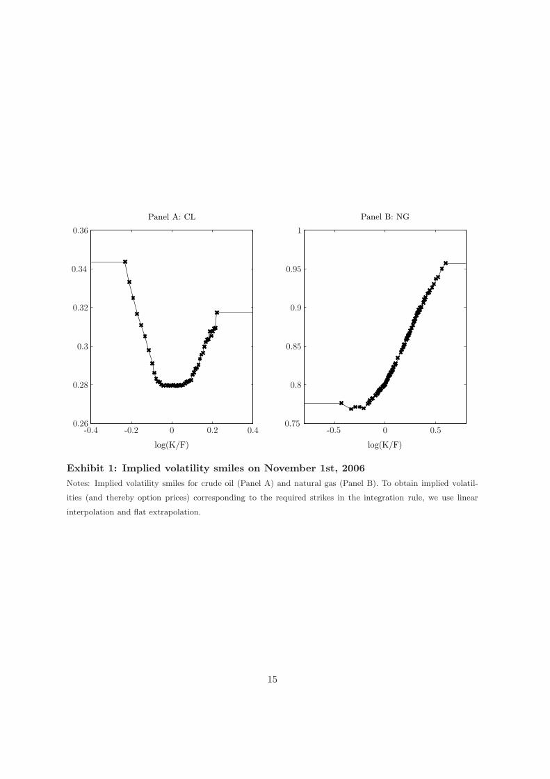
Jiang and Tian (2005) for an extensive discussion. Exhibit 1 shows the implied volatility smiles
on November 1st, 2006 and illustrates the interpolation/extrapolation scheme.
A synthetic 30 calendar day variance swap rate for the S&P 500 index (SPX) is easily
obtained by squaring the CBOE volatility index (VIX). This is because the VIX squared
approximates the conditional risk-neutral expectation of the realized 30 calendar day S&P 500
index variance. It is constructed along the lines of (3), using OTM S&P 500 index options along
with a particular discretization scheme as well as interpolation between two option maturities
to obtain a constant 30 calendar day maturity.13 Daily data on the VIX and SPX indices was
downloaded from the CBOE website.
4 Results
4.1 Properties of variance swap rates and realized variances
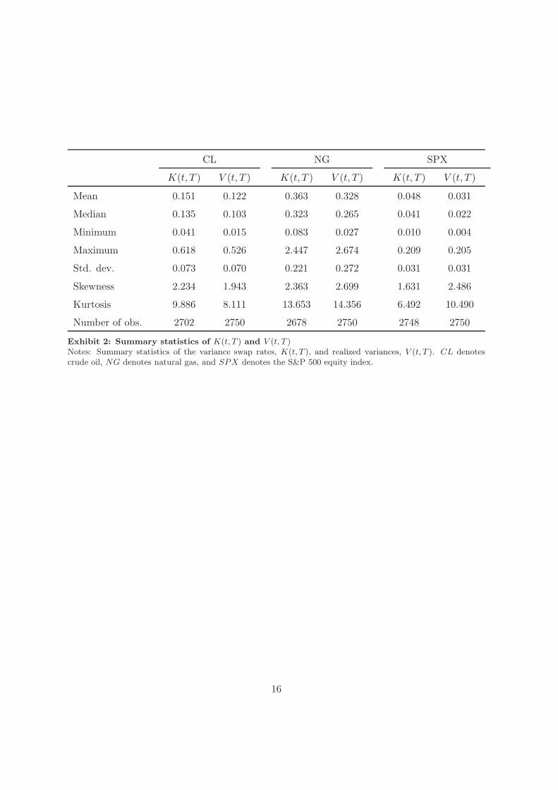
Exhibit 2 shows summary statistics of the variance swap rates and realized variances. For all
three assets, the mean variance swap rate is larger than the mean realized variance, reflecting
a negative variance risk premium in dollar terms on average. Natural gas is the most volatile
of the three markets. Not only is the variance of futures prices the largest on average, but the
volatility of the variance is also the largest. This holds true for both the variance swap rate
and realized variance. In fact, natural gas is the most volatile of all major commodity markets
except for electricity. Of the three markets analyzed, crude oil is the second most volatile,
while the S&P 500 index is the least volatile. In all three markets, the variance swap rate and
realized variance display positive skewness and excess kurtosis.14
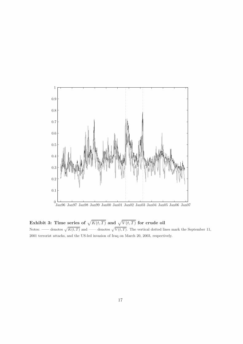
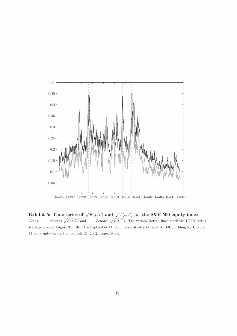
Exhibits 3 – 5 show the time-series of the variance swap rate and realized variance in
the three markets. Volatility in the crude oil market is very sensitive to geopolitical events
with the variance swap rate peaking after the September 11, 2001 terrorist attacks and in the
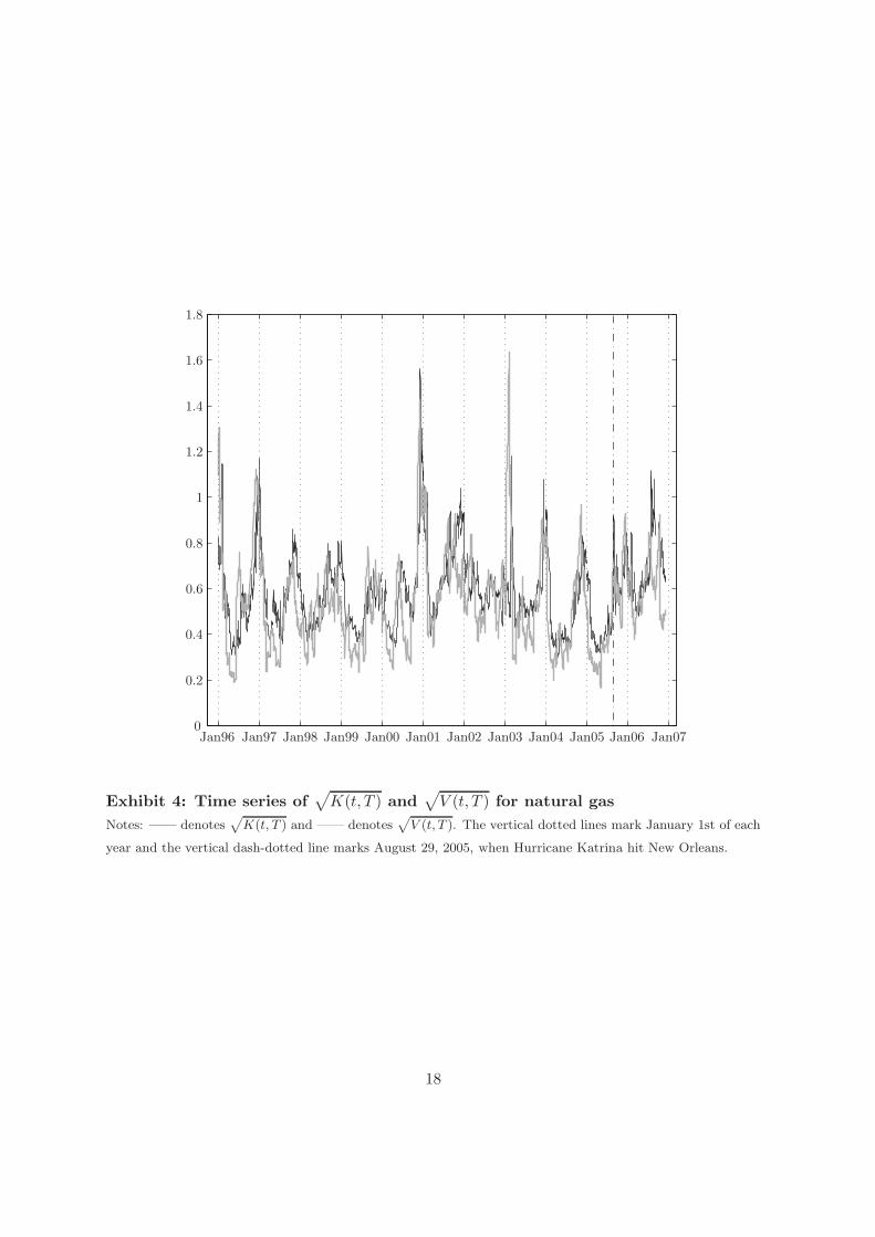
run-up to the US-led invasion of Iraq on March 20, 2003. Volatility in the natural gas market
displays a high degree of seasonality, with volatility typically peaking during the winter months
when demand for natural gas for heating purposes peaks. Since both supply and demand is
fairly price inelastic, higher-than-expected demand during the winter due to exceptionally cold
weather typically cause spikes in natural gas prices.15 The natural gas market is also exposed
to disruptions in supply. For instance, volatility rose sharply around Hurricane Katrina which
affected gas production in the Gulf of Mexico. For the S&P 500 index, the variance swap rate
7
peaks around the time LTCM disintegrated, after the September 11, 2001 terrorist attacks,
and after WorldCom filed for Chapter 11 bankruptcy protection.
Exhibit 6 displays the correlations between daily changes in variance swap rates, daily
changes in the estimated variances of the underlying contracts based on an EGARCH(1,1)
specification, and daily log returns of the underlying futures contracts. First, while changes in
the crude oil and natural gas variance swap rates display a small positive correlation (0.08),
both are virtually uncorrelated with changes in the variance swap rate for S&P 500 equity
index. Second, for crude oil, the correlation between futures returns and changes in variance
is negative but small (the correlation with changes in the variance swap rate is -0.04, and
the correlation with changes in the GARCH variance is -0.14). This is consistent with results
reported in Trolle and Schwartz (2009) who argue that crude oil volatility is largely unspanned
by the futures contracts.16 For natural gas, the correlation between futures returns and changes
in variance is moderately positive (the correlation with changes in the variance swap rate and
the GARCH variance is 0.36 and 0.43, respectively), suggesting that a larger component of
natural gas volatility is spanned by the futures contracts than is the case for crude oil. In
contrast, it is well-known that for the S&P500 index, the correlation between index returns
and changes in variance is highly negative (in our sample, the correlation with changes in the
variance swap rate and the GARCH variance is -0.77 and -0.80, respectively).17
4.2 Variance risk premia
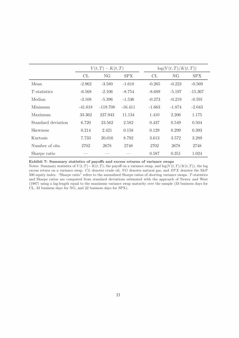
We consider a long position in a variance swap with a notional of 100 USD. Exhibit 7 shows
summary statistics of the dollar payoff, V (t, T )−K(t, T ), and log excess return, log(V (t, T )/K(t, T )),
for both energy commodities as well as the S&P 500 index. The T -statistics are adjusted for
the autocorrelation induced by the overlap in observations. The mean payoff and log excess
return is negative for all three assets. The mean payoff is most negative for natural gas (-3.58
USD), followed by crude oil (-2.96 USD) and the S&P 500 index (-1.62 USD). The mean log
excess return is most negative for the S&P 500 index (-56.9 percent) followed by crude oil
(-26.5 percent) and natural gas (-22.3 percent). The reason why the ranking between the
three assets changes, when considering returns instead of payoffs, is that the level of variance
is very different between the three assets. The mean payoffs and excess returns are statistically
significant in all three markets, with the T -statistics largest for S&P 500 index followed by
crude oil and natural gas.
8

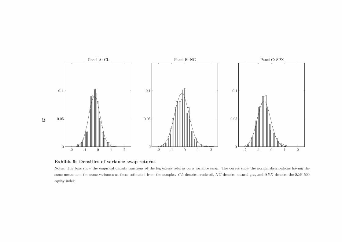
The distributions of payoffs exhibit fat tails for all three assets. It is fairly symmetric for
crude oil as well as the S&P 500 index but displays positive skewness for natural gas. In
contrast, the distributions of log excess returns are closer to normal although they do exhibit
positive skewness and excess kurtosis.
Finally, the table also reports the annualized Sharpe ratios (computed from standard de-
viations adjusted for the autocorrelation induced by the overlap in observations) of shorting
variance swaps. These are highest for the S&P 500 index (1.02) followed by crude oil (0.59) and
natural gas (0.35).18 To put these numbers into perspective, Duarte, Longstaff, and Yu (2007)
report annualized Sharpe ratios between 0.47 and 0.82 from shorting interest rate (specifically
cap) volatility, and Carr and Wu (2009) report annualized Sharpe ratios between 0 and 0.55
from shorting variance on selected individual stocks. Hence, although a strategy of shorting
variance in the two energy markets is not quite as attractive as shorting S&P 500 index vari-
ance, its performance seems comparable to a strategy of shorting interest rate volatility or
variance on individual stocks.
Exhibit 8 displays the three time series of log excess returns, and Exhibit 9 shows the
empirical density functions of log excess returns as well as the normal distributions having the
same means and the same variances as those estimated from the samples.
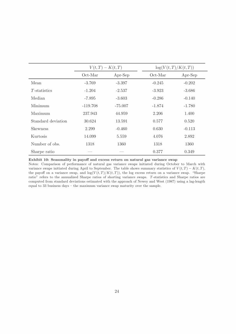
4.3 Seasonality in the natural gas variance risk premium
As mentioned above, natural gas volatility exhibits strong seasonality with volatility peaking
during the cold months. For instance, the mean variance swap rate during October to March is
44.3 percent compared with 28.6 percent during April to September. An interesting question
is whether the variance risk premium also exhibits seasonality. To this end, we compare
the performance of variance swaps initiated during October to March (the cold season) with
variance swaps initiated during April to September (the warm season). Exhibit 10 shows
summary statistics of the payoff, V (t, T )−K(t, T ), and log excess return, log(V (t, T )/K(t, T )).
The mean payoff is more negative during the cold season than during the warm season (-3.77
USD vs. -3.40 USD) and so is the mean log excess return (-24.5 percent vs. -20.2 percent).19
Also, the annualized Sharpe ratio of shorting natural gas variance swaps is higher during the
cold season than during the warm season (0.38 vs. 0.35). However, the difference between the
mean payoffs and the difference between the mean log excess returns during the cold and the
warm season is not statistically significant.20
9
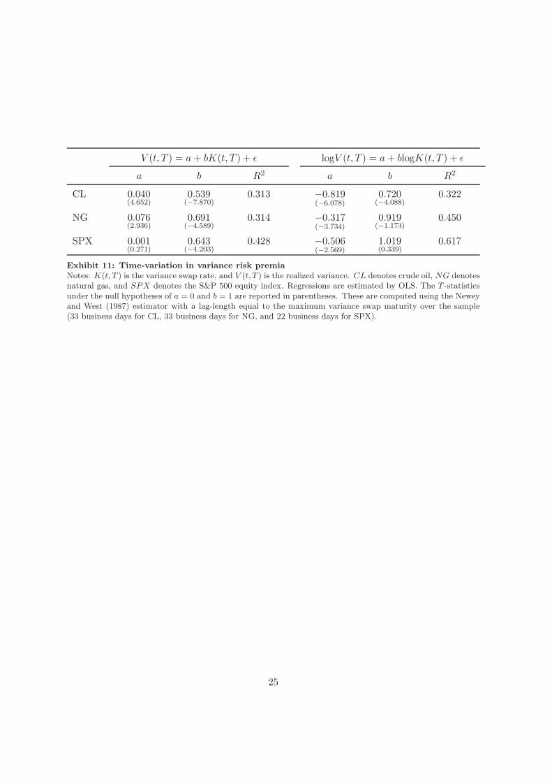
4.4 Time-variation in variance risk premia
As in Carr and Wu (2009) we test for time-variation in the variance risk premia by running
the following two regressions:
V (t, T ) = a + bK(t, T ) + ǫ (8)
and
logV (t, T ) = a + blogK(t, T ) + ǫ. (9)
Under the null hypothesis of constant variance risk premia in dollar terms, the slope in (8) is
one. Absence of variance risk premia in dollar terms would further imply that the intercept in
(8) is zero. Similarly, under the null hypothesis of constant variance risk premia in log return
terms, the slope in (9) is one. Zero variance risk premia in log return terms would further
imply that the intercept in (9) is zero.
Exhibit 11 displays estimates of both regressions. The regressions are estimated by OLS
with the T -statistics under the null hypotheses of a = 0 and b = 1 adjusted for the auto-
correlation induced by the overlap in observations. For both energy commodities, the slope
estimates in (8) are significantly less than one and are of similar magnitude. This indicates
that energy variance risk premia in dollar terms are time-varying and negatively correlated
with the level of the variance swap rate; i.e. variance risk premia in dollar terms tend to be-
come more negative when the variance swap rate increases. 21 In contrast, the slope estimates
in (9) are closer to one and only significantly different from one in the case of crude oil. This
shows that energy variance risk premia in log return terms, particularly in the case of natural
gas, are more constant over time and not highly correlated with the log variance swap rate.
The results for the S&P 500 index are very similar.
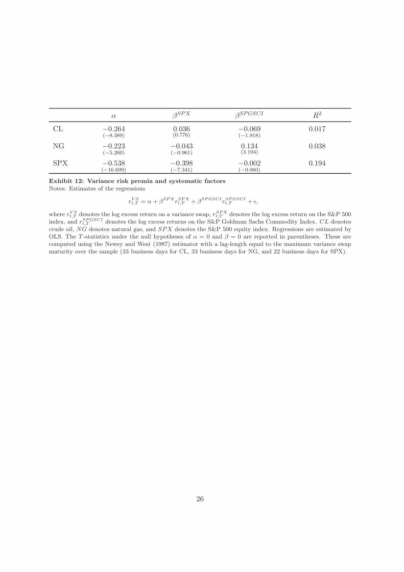
4.5 Fundamentals and variance risk premia
In this section, we first investigate the extent to which energy variance risk premia can be
explained within a standard asset pricing framework; in particular, whether the variance risk
premia reflect compensation for exposure to equity and commodity market risks. We regress
the log excess returns on variance swaps, rV St,T , on the contemporaneous log excess returns on
the S&P 500 index, rSPXt,T , and the log excess returns on the S&P Goldman Sachs Commodity
Index22, rSPGSCIt,T
rV St,T = α + βSPXrSPX
t,T + βSPGSCIrSPGSCIt,T + ǫ. (10)
10

Exhibit 12 shows that both energy variance swaps have an insignificant loading on the equity
market portfolio. However, both variance swaps load significantly on the commodity market
portfolio – crude oil with a negative sign and natural gas with a positive sign – but the R2s
are small and the alphas are significant and close to the unconditional means of log excess
returns reported in Exhibit 7. Hence, standard asset pricing models do not seem to be able
to explain energy variance risk premia.23 In the case of crude oil, this is consistent with the
finding in Trolle and Schwartz (2009) that variance risk is largely orthogonal to the underlying
futures market. The results are also consistent with studies that show the failure of standard
asset pricing models in accounting for risk premia in commodity futures; see, e.g. Jagannathan
(1985) for one such study.
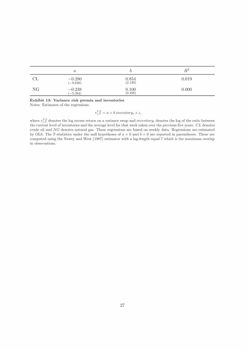
Next, we investigate if commodity specific factors may drive energy variance risk premia.
In particular, we consider inventories which have been shown to forecast excess returns on
commodity futures; see, e.g., Dincerler, Khokher, and Simin (2006) and Gorton, Hayashi, and
Rouwenhorst (2008) who find that futures risk premia tend to be larger when inventories are
low.24 We use weekly inventory data from the Energy Information Administration (EIA). For
crude oil we use the item “Crude Oil (Excluding SPR)” and for natural gas we use the item
“Working Gas in Underground Storage, Total Lower 48 States”. To control for seasonality in
inventories, we use relative inventories, which we define as the log of the ratio between the
level of inventories in a given week and the average level of inventories for that week over the
past five years. We regress the log excess returns on variance swaps from t to T , rV St,T , on the
relative inventory level at t25
rV St,T = a + b inventoryt + ǫ. (11)
Exhibit 13 shows that b has a positive sign in both regressions, implying that variance risk
premia tend to be more negative when relative inventories are low – similar to the findings
for futures risk premia. However, only in the case of crude oil is b significant and, even then,
the R2 is relatively low.26 Therefore, it seems that both systematic and commodity specific
factors have a difficult time accounting for energy variance risk premia.
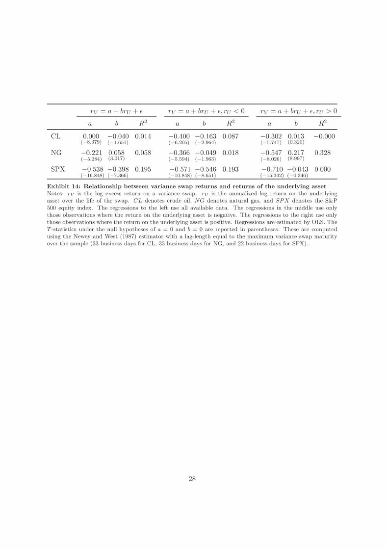
4.6 Option-like return profile of variance swaps
Exhibit 14 reports results from regressing the log excess return on a variance swap on the
annualized log return on the underlying asset over the life of the swap. In the crude oil
regression the relationship is negative but insignificant, while in the natural gas regression
11

there is a statistically significant positive relationship. In the S&P 500 regression there is a
statistically very significant negative relationship. This is consistent with the results in Section
4.1, that the correlation between daily underlying returns and changes in the GARCH variance
is negative but small for crude oil, moderately positive for natural gas and highly negative for
the S&P 500 index.
Studies on equity volatility have found that the negative correlation between index volatility
and index returns is mainly (or only) due to a negative correlation when index returns are
negative (see, e.g., Figlewski and Wang (2000)). This suggests that the relationship between
variance swap returns and returns of the underlying asset is non-linear in case of the S&P
500 index. Possibly, the relationship is also non-linear for the two energy commodities. To
see if this is the case, Exhibit 14 also reports results from running the regressions, first using
only those observations where the return on the underlying asset is negative, and then using
only those observations where the return on the underlying asset is positive. For natural gas
and the S&P 500 index, we find a strongly non-linear relationship. For natural gas, there is a
statistically highly significant positive relationship between variance swap returns and futures
returns, when the futures returns are positive, but a much weaker (negative) relationship when
the futures returns are negative. In contrast, for the S&P 500 index, there is a statistically
highly significant negative relationship between variance swap returns and the index returns,
when the index returns are negative, but an insignificant relationship when the index returns
are positive. For crude oil, the relationship is weaker although there is a statistically significant
negative relationship between variance swap returns and futures returns, when the futures
returns are negative, but virtually no relationship when the futures returns are positive.
Hence, the return profile of a natural gas variance swap resembles that of a call option,
while the return profile of an S&P 500 index variance swap resembles the return profile of
a put option. The return profile of a crude oil variance swap has a less distinctive pattern,
although if anything it also resembles the return profile of a put option. This is also evident
from Exhibit 15, which shows scatter-plots of log excess variance swap returns vs. annualized
contemporaneous log returns of the underlying assets.
5 Conclusion
This paper has investigated variance risk premia in energy commodities, particularly crude
oil and natural gas, using a robust model-independent approach. The analysis is based on 11
12
years of daily data on futures and options trading on NYMEX.
We find that the average variance risk premia are negative for both energy commodities,
but more strongly statistically significant for crude oil than for natural gas. In the case
of natural gas, we find some degree of seasonality in the risk premium, although it is not
statistically significant. Furthermore, energy variance risk premia in dollar terms are time-
varying and correlated with the level of the variance swap rate, while energy variance risk
premia in return terms, particularly in the case of natural gas, are much less correlated with
the (log) variance swap rate. Moreover, it is difficult to explain the level and variation in
energy variance risk premia with systematic factors (returns on equity and commodity market
portfolios) or commodity specific factors (inventories). Finally, the return profile of a natural
gas variance swap resembles that of a call option, while the return profile of a crude oil variance
swap has a less distinctive pattern, although if anything it resembles the return profile of a
put option.
During our sample period, the annualized Sharpe ratios from shorting variance is 0.59 for
crude oil and 0.35 for natural gas. This is not nearly as high as the annualized Sharpe ratio of
shorting S&P 500 index variance, but is comparable to the annualized Sharpe ratios, reported
in other studies, of shorting interest rate volatility or variance on individual stocks.
In future work we plan to explore the economic underpinnings of the negative energy
variance risk premia and their dynamics. It will also be interesting to investigate how energy
variance swaps fit into diversified commodity portfolios.
Appendix
Assume that the risk-neutral dynamics of the futures price F (t, T1) is given by the following
jump-diffusion process:
dF (t, T1)
F (t, T1)=√
v(t)dW (t) + (ex − 1)dN(t) −∫
R
(ex − 1)f(x)dxλ(t)dt, (12)
where W (t) is a Wiener process, v(t) is the instantaneous variance of the diffusion component,
N(t) is a Poisson process with time-varying intensity λ(t), x is the jump size conditional on a
jump occurring, and f(x) is the density of the jump-size distribution. By Ito’s lemma
dlogF (t, T1) = −1
2v(t)dt +
√v(t)dW (t) + xdN(t) −
∫
R
(ex − 1)f(x)dxλ(t)dt, (13)
13
so that
logF (T, T1) = logF (t, T1) −1
2
∫ T
t
v(s)ds +
∫ T
t
√v(s)dW (s) +
N(T )∑
i=1
x −∫
R
(ex − 1)f(x)dx
∫ T
t
λ(s)ds.(14)
The annualized realized quadratic variation of futures returns over the period [t, T ], T ≤ T1,
is given by
V (t, T ) =1
T − t
∫ T
t
v(s)ds +
N(T )∑
i=1
x2
. (15)
Combining (14) and (15) and taking expectations, we obtain
EQt [V (t, T )] = − 2
T − tEQ
t
[log
(F (T, T1)
F (t, T1)
)]− 2
T − t
∫
R
(ex − 1 − x − 1
2x2
)f(x)dx
∫ T
t
λ(s)ds(16)
From Carr and Madan (2001) it follows that for any fixed Z we can write any twice continuously
differentiable function g of F (T, T1) as
g(F (T, T1)) = g(Z) + g′(Z)(F (T, T1) − Z) +
∫ Z
0g′′(X)(X − F (T, T1))
+dX
+
∫∞
Z
g′′(X)(F (T, T1) − X)+dX. (17)
In particular, with g(F ) = logF and Z = F (t, T1), taking expectations, and rearranging, we
obtain
EQt
[log
(F (T, T1)
F (t, T1)
)]= − 1
B(t, T )
(∫ F (t,T1)
0
P(t, T, T1,X)
X2dX +
∫∞
F (t,T1)
C(t, T, T1,X)
X2dX
)(18)
Inserting this expression in (16) and ignoring the jump-induced term, which Gatheral (2006)
and Carr and Wu (2009) argue is very small for plausible parameters, gives (3).
14
Panel A: CL
log(K/F)
Panel B: NG
log(K/F)
-0.5 0 0.5-0.4 -0.2 0 0.2 0.40.75
0.8
0.85
0.9
0.95
1
0.26
0.28
0.3
0.32
0.34
0.36
Exhibit 1: Implied volatility smiles on November 1st, 2006
Notes: Implied volatility smiles for crude oil (Panel A) and natural gas (Panel B). To obtain implied volatil-
ities (and thereby option prices) corresponding to the required strikes in the integration rule, we use linear
interpolation and flat extrapolation.
15
CL NG SPX
K(t, T ) V (t, T ) K(t, T ) V (t, T ) K(t, T ) V (t, T )
Mean 0.151 0.122 0.363 0.328 0.048 0.031
Median 0.135 0.103 0.323 0.265 0.041 0.022
Minimum 0.041 0.015 0.083 0.027 0.010 0.004
Maximum 0.618 0.526 2.447 2.674 0.209 0.205
Std. dev. 0.073 0.070 0.221 0.272 0.031 0.031
Skewness 2.234 1.943 2.363 2.699 1.631 2.486
Kurtosis 9.886 8.111 13.653 14.356 6.492 10.490
Number of obs. 2702 2750 2678 2750 2748 2750
Exhibit 2: Summary statistics of K(t, T ) and V (t, T )Notes: Summary statistics of the variance swap rates, K(t, T ), and realized variances, V (t, T ). CL denotescrude oil, NG denotes natural gas, and SPX denotes the S&P 500 equity index.
16
replacemen
Jan96 Jan97 Jan98 Jan99 Jan00 Jan01 Jan02 Jan03 Jan04 Jan05 Jan06 Jan070
0.1
0.2
0.3
0.4
0.5
0.6
0.7
0.8
0.9
1
Exhibit 3: Time series of√
K(t, T ) and√
V (t, T ) for crude oil
Notes: —— denotes√
K(t, T ) and —— denotes√
V (t, T ). The vertical dotted lines mark the September 11,
2001 terrorist attacks, and the US-led invasion of Iraq on March 20, 2003, respectively.
17
Jan96 Jan97 Jan98 Jan99 Jan00 Jan01 Jan02 Jan03 Jan04 Jan05 Jan06 Jan070
0.2
0.4
0.6
0.8
1
1.2
1.4
1.6
1.8
Exhibit 4: Time series of√
K(t, T ) and√
V (t, T ) for natural gas
Notes: —— denotes√
K(t, T ) and —— denotes√
V (t, T ). The vertical dotted lines mark January 1st of each
year and the vertical dash-dotted line marks August 29, 2005, when Hurricane Katrina hit New Orleans.
18
Jan96 Jan97 Jan98 Jan99 Jan00 Jan01 Jan02 Jan03 Jan04 Jan05 Jan06 Jan070
0.05
0.1
0.15
0.2
0.25
0.3
0.35
0.4
0.45
0.5
Exhibit 5: Time series of√
K(t, T ) and√
V (t, T ) for the S&P 500 equity index
Notes: —— denotes√
K(t, T ) and —— denotes√
V (t, T ). The vertical dotted lines mark the LTCM crisis
starting around August 31, 1998, the September 11, 2001 terrorist attacks, and WorldCom filing for Chapter
11 bankruptcy protection on July 21, 2002, respectively.
19

∆KCL ∆KNG ∆KSPX ∆σ2CL ∆σ2
NG ∆σ2SPX RCL RNG RSPX
∆KCL 1.000
∆KNG 0.079 1.000
∆KSPX 0.003 -0.018 1.000
∆σ2CL 0.337 0.031 -0.021 1.000
∆σ2NG 0.013 0.409 0.027 0.060 1.000
∆σ2SPX 0.003 0.024 0.715 0.000 0.027 1.000
RCL -0.035 0.079 -0.004 -0.144 0.139 -0.013 1.000
RNG 0.006 0.358 -0.014 -0.014 0.425 0.025 0.310 1.000
RSPX -0.022 -0.008 -0.766 0.027 -0.008 -0.799 -0.022 -0.021 1.000
Exhibit 6: Correlations
Notes: Correlations between daily changes in variance swap rates (∆K), daily changes in the estimated variancesof the underlying assets based on an EGARCH(1,1) specification (∆σ2), and daily log returns of the underlyingassets (R). CL denotes crude oil, NG denotes natural gas, and SPX denotes the S&P 500 equity index.
20
V (t, T ) − K(t, T ) log(V (t, T )/K(t, T ))
CL NG SPX CL NG SPX
Mean -2.962 -3.580 -1.618 -0.265 -0.223 -0.569
T -statistics -6.568 -2.106 -8.754 -8.689 -5.197 -15.367
Median -3.108 -5.396 -1.536 -0.273 -0.219 -0.591
Minimum -41.618 -119.708 -16.411 -1.663 -1.874 -2.043
Maximum 33.362 237.943 11.134 1.410 2.206 1.175
Standard deviation 6.720 23.562 2.582 0.437 0.549 0.504
Skewness 0.214 2.421 0.158 0.129 0.299 0.393
Kurtosis 7.733 20.016 8.792 3.613 3.572 3.289
Number of obs. 2702 2678 2748 2702 2678 2748
Sharpe ratio — — — 0.587 0.351 1.024
Exhibit 7: Summary statistics of payoffs and excess returns of variance swaps
Notes: Summary statistics of V (t, T )−K(t, T ), the payoff on a variance swap, and log(V (t, T )/K(t, T )), the logexcess return on a variance swap. CL denotes crude oil, NG denotes natural gas, and SPX denotes the S&P500 equity index. “Sharpe ratio” refers to the annualized Sharpe ratios of shorting variance swaps. T -statisticsand Sharpe ratios are computed from standard deviations estimated with the approach of Newey and West(1987) using a lag-length equal to the maximum variance swap maturity over the sample (33 business days forCL, 33 business days for NG, and 22 business days for SPX).
21

Panel A: CL Panel B: NG Panel C: SPX
Jan96 Jan99 Jan02 Jan05Jan96 Jan99 Jan02 Jan05Jan96 Jan99 Jan02 Jan05-2
-1
0
1
2
-2
-1
0
1
2
-2
-1
0
1
2
Exhibit 8: Time series of variance swap returns
Notes: Time series of log (V (t, T )/K(t, T )), the log excess returns on a variance swap. CL denotes crude oil, NG denotes natural gas, and SPX denotes the
S&P 500 equity index. For crude oil, the vertical dotted lines mark the September 11, 2001 terrorist attacks, and the US-led invasion of Iraq on March 20,
2003, respectively. For natural gas, the vertical dotted lines mark January 1st of each year and the vertical dash-dotted line marks August 29, 2005, when
Hurricane Katrina hit New Orleans. For the S&P 500 index, the vertical dotted lines mark the LTCM crisis starting around August 31, 1998, the September
11, 2001 terrorist attacks, and WorldCom filing for Chapter 11 bankruptcy protection on July 21, 2002, respectively.
22
Panel A: CL Panel B: NG Panel C: SPX
-2 -1 0 1 2-2 -1 0 1 2-2 -1 0 1 20
0.05
0.1
0
0.05
0.1
0
0.05
0.1
Exhibit 9: Densities of variance swap returns
Notes: The bars show the empirical density functions of the log excess returns on a variance swap. The curves show the normal distributions having the
same means and the same variances as those estimated from the samples. CL denotes crude oil, NG denotes natural gas, and SPX denotes the S&P 500
equity index.
23
V (t, T ) − K(t, T ) log(V (t, T )/K(t, T ))
Oct-Mar Apr-Sep Oct-Mar Apr-Sep
Mean -3.769 -3.397 -0.245 -0.202
T -statistics -1.204 -2.537 -3.923 -3.686
Median -7.895 -3.603 -0.286 -0.140
Minimum -119.708 -75.007 -1.874 -1.780
Maximum 237.943 44.959 2.206 1.400
Standard deviation 30.624 13.591 0.577 0.520
Skewness 2.299 -0.460 0.630 -0.113
Kurtosis 14.099 5.559 4.076 2.892
Number of obs. 1318 1360 1318 1360
Sharpe ratio — — 0.377 0.349
Exhibit 10: Seasonality in payoff and excess return on natural gas variance swap
Notes: Comparison of performance of natural gas variance swaps initiated during October to March withvariance swaps initiated during April to September. The table shows summary statistics of V (t, T ) − K(t, T ),the payoff on a variance swap, and log(V (t, T )/K(t, T )), the log excess return on a variance swap. “Sharperatio” refers to the annualized Sharpe ratios of shorting variance swaps. T -statistics and Sharpe ratios arecomputed from standard deviations estimated with the approach of Newey and West (1987) using a lag-lengthequal to 33 business days – the maximum variance swap maturity over the sample.
24
V (t, T ) = a + bK(t, T ) + ǫ logV (t, T ) = a + blogK(t, T ) + ǫ
a b R2 a b R2
CL 0.040(4.652)
0.539(−7.870)
0.313 −0.819(−6.078)
0.720(−4.088)
0.322
NG 0.076(2.936)
0.691(−4.589)
0.314 −0.317(−3.734)
0.919(−1.173)
0.450
SPX 0.001(0.271)
0.643(−4.203)
0.428 −0.506(−2.569)
1.019(0.339)
0.617
Exhibit 11: Time-variation in variance risk premia
Notes: K(t, T ) is the variance swap rate, and V (t, T ) is the realized variance. CL denotes crude oil, NG denotesnatural gas, and SPX denotes the S&P 500 equity index. Regressions are estimated by OLS. The T -statisticsunder the null hypotheses of a = 0 and b = 1 are reported in parentheses. These are computed using the Neweyand West (1987) estimator with a lag-length equal to the maximum variance swap maturity over the sample(33 business days for CL, 33 business days for NG, and 22 business days for SPX).
25
α βSPX βSPGSCI R2
CL −0.264(−8.389)
0.036(0.776)
−0.069(−1.918)
0.017
NG −0.223(−5.260)
−0.043(−0.961)
0.134(3.194)
0.038
SPX −0.538(−16.699)
−0.398(−7.341)
−0.002(−0.060)
0.194
Exhibit 12: Variance risk premia and systematic factors
Notes: Estimates of the regressions
rV St,T = α + βSPXrSPX
t,T + βSPGSCIrSPGSCIt,T + ǫ,
where rV St,T denotes the log excess return on a variance swap, rSPX
t,T denotes the log excess return on the S&P 500index, and rSPGSCI
t,T denotes the log excess returns on the S&P Goldman Sachs Commodity Index. CL denotescrude oil, NG denotes natural gas, and SPX denotes the S&P 500 equity index. Regressions are estimated byOLS. The T -statistics under the null hypotheses of α = 0 and β = 0 are reported in parentheses. These arecomputed using the Newey and West (1987) estimator with a lag-length equal to the maximum variance swapmaturity over the sample (33 business days for CL, 33 business days for NG, and 22 business days for SPX).
26
a b R2
CL −0.280(−9.626)
0.854(2.120)
0.019
NG −0.238(−5.394)
0.100(0.498)
0.000
Exhibit 13: Variance risk premia and inventories
Notes: Estimates of the regressions
rV St,T = a + b inventoryt + ǫ,
where rV St,T denotes the log excess return on a variance swap and inventoryt denotes the log of the ratio between
the current level of inventories and the average level for that week taken over the previous five years. CL denotescrude oil and NG denotes natural gas. These regressions are based on weekly data. Regressions are estimatedby OLS. The T -statistics under the null hypotheses of a = 0 and b = 0 are reported in parentheses. These arecomputed using the Newey and West (1987) estimator with a lag-length equal 7 which is the maximum overlapin observations.
27
rV = a + brU + ǫ rV = a + brU + ǫ, rU < 0 rV = a + brU + ǫ, rU > 0
a b R2 a b R2 a b R2
CL 0.000(−8.379)
−0.040(−1.651)
0.014 −0.400(−6.205)
−0.163(−2.964)
0.087 −0.302(−5.747)
0.013(0.320)
−0.000
NG −0.221(−5.284)
0.058(3.017)
0.058 −0.366(−5.594)
−0.049(−1.963)
0.018 −0.547(−8.026)
0.217(8.997)
0.328
SPX −0.538(−16.848)
−0.398(−7.366)
0.195 −0.571(−10.848)
−0.546(−8.651)
0.193 −0.710(−15.342)
−0.043(−0.346)
0.000
Exhibit 14: Relationship between variance swap returns and returns of the underlying asset
Notes: rV is the log excess return on a variance swap. rU is the annualized log return on the underlyingasset over the life of the swap. CL denotes crude oil, NG denotes natural gas, and SPX denotes the S&P500 equity index. The regressions to the left use all available data. The regressions in the middle use onlythose observations where the return on the underlying asset is negative. The regressions to the right use onlythose observations where the return on the underlying asset is positive. Regressions are estimated by OLS. TheT -statistics under the null hypotheses of a = 0 and b = 0 are reported in parentheses. These are computedusing the Newey and West (1987) estimator with a lag-length equal to the maximum variance swap maturityover the sample (33 business days for CL, 33 business days for NG, and 22 business days for SPX).
28

Panel A: CL
r V
rU
Panel B: NG
r VrU
Panel C: SPX
r V
rU
-4 -2 0 2 4-10 -5 0 5 10-5 0 5-2.5
-2
-1.5
-1
-0.5
0
0.5
1
1.5
-2
-1.5
-1
-0.5
0
0.5
1
1.5
2
2.5
-2
-1.5
-1
-0.5
0
0.5
1
1.5
Exhibit 15: Returns on variance swaps vs. returns of the underlying assets
Notes: rV is the log excess return on a variance swap. rU is the annualized log return on the underlying asset over the life of the swap. CL denotes crude
oil, NG denotes natural gas, and SPX denotes the S&P 500 equity index. In each panel, the grey line to the left is the regression fit using only those
observations where the return on the underlying asset is negative, while the grey line to the right is the regression fit using only those observations where
the return on the underlying asset is positive.
29
Notes
1 See Davis (2006).
2 The S&P GSCI is comprised of 24 commodities with the weight of each commodity
determined by their relative levels of world production over the past five years. The DJ-
AIGCI is comprised of 19 commodities with the weight of each component determined by
liquidity and world production values, with liquidity being the dominant factor. In addition,
for this index, no single commodity may constitute more than 15 percent and no sector may
constitute more than 33 percent. Crude oil and natural gas are the largest components in both
indices. In 2007, their weights were 51.30 percent and 6.71 percent, respectively, in the S&P
GSCI and 13.88 percent and 11.03 percent, respectively, in the DJ-AIGCI.
3Upon revising the paper, we attempted to extend the sample to 2009. However, NYMEX
(now part of CME group) was not able to provide us with the latest data.
4The Chicago Board Options Exchange (CBOE) recently introduced a Crude Oil Volatility
Index (ticker symbol OVX). This index also measures the conditional risk-neutral expectation
of crude oil variance, but is computed from a cross-section of listed options on the United
States Oil Fund (ticker symbol USO), which tracks the price of WTI as closely as possible.
However, since USO options only started trading in May, 2007, the history of this index is too
short to investigate the crude oil variance risk premium.
5 Bakshi and Kapadia (2003b) also find that variance risk premia for individual stocks are
less negative than for the S&P 500 index.
6 Carr and Wu (2009)) provide a more general derivation for the case where the underlying
asset is a semi-martingale.
7See, e.g., Gatheral (2006) p. 137. Whether one computes variance in terms of log returns
or arithmetic returns and whether one demeans returns or not, makes little difference to the
results.
8 Crude oil and natural gas trade in units of 1,000 barrels and 10,000 million British thermal
units (mmBtu), respectively. Prices are quoted as US dollars and cents per barrel or mmBtu.
30
9 Settlement prices for all contracts are determined by a “Settlement Price Committee” at
the end of regular trading hours and represent a very accurate measure of the true market
prices at the time of close. Settlement prices are widely scrutinized by all market participants
since they are used for marking to market all account balances.
10 For crude oil, options expire three business days prior to the expiration of the underlying
futures contract, which in turn expires on the third business day prior to the 25th calendar
day of the month preceding the delivery month (if the 25th calendar day is a non-business day,
expiration is on the third business day prior to the business day preceding the 25th calendar
day). For natural gas, options expire one business day prior to the expiration of the underlying
futures contract, which in turn expires on the third business day prior to the delivery month.
11 NYMEX does list European-style options on both commodities. However, the trading
history is much shorter and liquidity is much lower than for the American-style options.
12 The idea is, for each option, to assume that the price of the underlying futures contract
follows a geometric Brownian motion. With this assumption, American options can be priced
using the Barone-Adesi and Whaley (1987) formula. Inverting this formula for a given Amer-
ican option price yields an implied volatility, from which the associated European option can
be priced with the Black (1976a) formula.
13 The CBOE webiste contains the details of the construction.
14 Note that due to missing options data, there are fewer than 2750 observations for the
variance swap rates.
15 Since natural gas is also used for electricity generation, higher-than-expected air condi-
tioning demand during the summer due to exceptionally warm weather may also cause sharp
increases in natural gas prices.
16 Trolle and Schwartz (2009) estimate various stochastic volatility HJM models on crude oil
futures and options data and find small negative correlations in the range −0.10 to 0 between
innovations to volatility and spot returns. Since spot returns are very highly correlated with
returns on the front futures contract, this is consistent with the correlations found here.
17 This is the so-called “leverage effect”, first discussed by Black (1976b), although changes in
leverage is probably not the main explanation for the negative correlation – see, e.g., Figlewski
31
and Wang (2000).
18 In case of the S&P 500 index, the estimated annualized Sharpe ratio is very close to the
0.98 reported by Carr and Wu (2009).
19 Note that due to large differences in the standard deviation of the payoff, the mean payoff
is statistically insignificant during the cold season but statistically significant during the warm
season. In contrast, the mean log excess return is more strongly statistically significant during
the cold season than during the warm season. Note also that both the payoff distribution and
the log excess return distribution are positively skewed during the cold season, while negatively
skewed during the warm season.
20 To see this, let µ1 and µ2 denote the estimated mean payoffs or mean log excess returns
during the cold and the warm season, respectively. Furthermore, let σ21 and σ2
2 denote the
variances estimated with the approach of Newey and West (1987) using 33 lags, and let n1
and n2 denote the number of observations. Then, under the null-hypothesis of equal means,
and assuming independence between the cold and the warm season, we have that
T =µ1 − µ2√
σ21/n1 + σ2
2/n2
(19)
is asymptotically standard normally distributed. When testing for equality between the mean
payoffs, we have T = −0.11, and when testing for equality between the mean log excess returns,
we have T = −0.51. Hence, in neither case can we reject the null-hypothesis of equality.
21A number of studies (see, e.g., Canina and Figlewski (1993)), using mostly equity data,
have run regressions similar to (8) to test the extent to which implied volatility contains
information about future realized volatility. These studies generally find b to be significantly
less than one, implying that implied volatility is a biased forecast of future realized volatility.
While this is consistent with a time-varying volatility risk premium, it is sometimes interpreted
as evidence for market frictions or even options trader irrationality.
22For the S&P GSCI, the excess return is computed from the S&P GSCI Excess Return
index which measures the return from investing in nearby S&P GSCI futures and rolling them
forward each month.
23 As already noted by Carr and Wu (2006) and Carr and Wu (2009), it also does not
seem to be able to explain the equity index variance risk premium, although the equity index
32
variance swap has a significant negative loading on the equity market portfolio.
24Another commodity specific factor that has been investigated in the literature is the net
position of hedgers in the futures market; see, e.g., Bessembinder (1992) and de Roon, Nijman,
and Veld (2000) who link futures risk premia to this factor. In a similar vein, it would
be interesting to investigate if energy variance risk premia vary with the net positions of
hedgers in the crude oil and natural gas options market. Unfortunately, while the Commodity
Futures Trading Commission does publish some information about the net position of hedgers
in options markets, this is done on a futures-equivalent basis, which implies that it groups
together long call and short put positions as well as long put and short call positions. For
our purpose, we would need information about the extent to which hedgers are long calls and
puts, and this information is not readily available.
25Inventory data for a given week are released by the EIA on the following Wednesday in
the case of crude oil and Thursday in the case of natural gas. We therefore match inventories
with returns on variance swaps initiated the following Wednesday or Thursday.
26For robustness, we also ran the regressions with absolute, rather than relative, inventories
but found no significant relationships with variance risk premia.
33
References
Bakshi, G. and N. Kapadia (2003a). Delta-hedged gains and the negative market volatility
risk premium. Review of Financial Studies 16, 527–566.
Bakshi, G. and N. Kapadia (2003b). Volatility risk premium embedded in individual equity
options: Some new insights. Journal of Derivatives 11, 45–54.
Barone-Adesi, G. and R. Whaley (1987). Efficient analytic approximation of american option
values. Journal of Finance 42, 301–320.
Bessembinder, H. (1992). Systematic risk, hedging pressure, and risk premiums in futures
markets. Review of Financial Studies 5, 637–667.
Black, F. (1976a). The pricing of commodity contracts. Journal of Financial Economics 3,
167–179.
Black, F. (1976b). Studies of stock price volatility changes. Proceedings of the 1976 Meetings
of the American Statistical Association, Business and Economic Statistics Section 1,
177–181.
Bollerslev, T., M. Gibson, and H. Zhou (2004). Dynamic estimation of volatility risk premia
and investor risk aversion from option-implied and realized volatilities. Working paper,
Duke University and Federal Reserve Board.
Bondarenko, O. (2004). Market price of variance risk and performance of hedge funds.
Working paper, University of Illinois at Chicago.
Britten-Jones, M. and A. Neuberger (2000). Option prices, implied price processes, and
stochastic volatility. Journal of Finance 55, 839–866.
Broadie, M., M. Chernov, and M. Johannes (2007). Model specification and risk premiums:
Evidence from futures options. Journal of Finance 62, 1453–1490.
Canina, L. and S. Figlewski (1993). The informational content of implied volatility. Review
of Financial Studies 6, 659–681.
Carr, P. and D. Madan (1998). Towards a theory of volatility trading. in, Robert Jarrow,
eds.: Risk Book on Volatility, Risk, New York.
Carr, P. and D. Madan (2001). Optimal positioning in derivatives securities. Quantitative
Finance 1, 19–37.
34

Carr, P. and L. Wu (2006). A tale of two indices. Journal of Derivatives 13, 13–29.
Carr, P. and L. Wu (2009). Variance risk premia. Review of Financial Studies 22, 1311–1341.
Coval, J. and T. Shumway (2001). Expected option returns. Journal of Finance 56, 983–
1009.
Davis, A. (2006). How giant bets on natural gas sank brash hedge-fund trader. Wall Street
Journal September 19.
de Roon, F., T. Nijman, and C. Veld (2000). Hedging pressure effects in futures markets.
Journal of Finance 55, 1437–1456.
Demeterfi, K., E. Derman, M. Kamal, and J. Zou (1999). A guide to volatility and variance
swaps. Journal of Derivatives 6, 9–32.
Dincerler, C., Z. Khokher, and T. Simin (2006). An empirical analysis of commodity con-
venience yields. Working paper, Pennsylvania State University.
Doran, J. S. and E. I. Ronn (2008). Computing the market price of volatility risk in the
energy commodity markets. Journal of Banking and Finance 32, 2541–2552.
Duarte, J., F. Longstaff, and F. Yu (2007). Risk and return in fixed income arbitrage:
Nickels in front of a steamroller. Review of Financial Studies 20, 769–811.
Erb, C. and C. Harvey (2006). The strategic and tactical value of commodity futures.
Financial Analysts Journal 62, 69–97.
Figlewski, S. and X. Wang (2000). Is the ‘Leverage Effect’ a Leverage Effect? Working
paper, NYU Stern School of Business.
Gatheral, J. (2006). The Volatility Surface. Wiley.
Gorton, G., F. Hayashi, and G. K. Rouwenhorst (2008). The fundamentals of commodity
futures returns. Working paper, Yale University.
Gorton, G. and G. K. Rouwenhorst (2006). Facts and fantasies about commodity futures.
Financial Analysts Journal 62, 47–68.
Ibbotson (2006). Strategic asset allocation and commodities. March 27.
Jagannathan, R. (1985). An investigation of commodity futures prices using the
consumption-based intertemporal capital asset pricing model. Journal of Finance 40,
175–191.
35
Jiang, G. and Y. Tian (2005). The model-free implied volatility and its information content.
Review of Financial Studies 18, 1305–1342.
Kat, H. and R. Oomen (2007a). What every investor should know about commodities, Part
I. Journal of Investment Management 5, 4–28.
Kat, H. and R. Oomen (2007b). What every investor should know about commodities, Part
II. Journal of Investment Management 5, 40–64.
Newey, W. and K. West (1987). A simple, positive semi-definit, heteroscedasticity and
autocorrelation consistent covariance matrix. Econometrica 55, 703–708.
Pan, J. (2002). The jump-risk premia implicit in options: Evidence from an integrated
time-series study. Journal of Financial Economics 63, 3–50.
Trolle, A. B. and E. S. Schwartz (2009). Unspanned stochastic volatility and the pricing of
commodity derivatives. Review of Financial Studies 22, 4423–4461.
36