variables important for bankruptcy prediction - a...

Bachelor Thesis

Variables Important for Bankruptcy Prediction: A Logit

Binary Approach

Bachelor’s Program in Economics

Lund University

Autumn 2012

Authors:

Oscar Taurell

Viktor Augustsson

Tutor:

Dr. Hossein Asgharian

2

Abstract

The purpose of this bachelor thesis is to estimate our own bankruptcy prediction model using

logit binary data. Our choice of variables is based on Altman’s Z-score model 1968. A

comparison is then done between results in Altman and our findings. We perform our

estimates on 114 listed Nordic companies, where 37 of them went bankrupt during 2002-

2012.

We find that our estimated model can categorize defaulting and non-defaulting firms

best, two years prior to the event of bankruptcy. This is done with a 76,8 per cent accuracy.

Finally, we show that our model can predict bankruptcy of Nordic firms better than Altman’s

Z-score model.

Keywords: bankruptcy prediction, Z-score model, logit binary, maximum likelihood

3

Table of Contents

I. Introduction.............................................................................................................................5

A. Background and Motivation............................................................................................5

B. Purpose............................................................................................................................6

C. Delimitations...................................................................................................................6

D. Outline of the Thesis.......................................................................................................6

II. Previous Research..................................................................................................................7

III. Methodology.........................................................................................................................7

A. Altman’s Z-score Model.................................................................................................8

B. Variables in Altman’s Z-score Model.............................................................................9

C. The Logit Binary Model...............................................................................................10

D. Maximum Likelihood Model........................................................................................12

E. Maximum Likelihood in the Logit Model....................................................................13

IV. Model Validation Tests.......................................................................................................14

A. Criterion for Variable Selection....................................................................................14

B. Type I and type II Error................................................................................................14

C. Chi-Squared Test...........................................................................................................15

D. Multicollinearity............................................................................................................16

E. Heteroskedasticity.........................................................................................................16

F. Hypothesis Testing........................................................................................................17

V. Analysis................................................................................................................................17

A. Data Analysis................................................................................................................17

i. Time Fluctuating Factors in our Sample...........................................................18

ii. Analysis of the Country Selection....................................................................19

iii. Logit Transformation........................................................................................19

B. Test for Misspecification..............................................................................................20

i. Test of the Model’s Accuracy...........................................................................20

4

ii. Test of the Parameters....................................................................................23

C. Our Bankruptcy Prediction Model................................................................................25

i. Significance of 𝛽!...............................................................................................25

ii. Significance of 𝛽!..............................................................................................27

iii. Marginal effects.................................................................................................28

D. Comparison to Altman’s Marginal Effects...................................................................30

i. Chi-Squared Test of Altman’s Z-score Model....................................................31

VI. Conclusion..........................................................................................................................31

References.....................................................................................................................34

i. Other References.................................................................................................35

5

I. Introduction

Throughout this chapter we give background information together with our motivation. We

then outline the purpose of the thesis, discuss the thesis delimitations and finally outline

previous research on the same topic.

A. Background and Motivation

The uncertain economic environment during the recent years have stressed the importance of

managing credit risk, i.e. the “risk that a borrower may default on his obligations; a danger

that interest payments and repayment of principal will not occur”.1 During the financial

crisis of 2008 and 2009 the correlated defaults and the resulting bankruptcy wave evolved to a

systemic risk in the financial sector, which in turn had a major negative impact on the entire

global economy. A proper prediction of firm bankruptcies might therefore be extremely

important and of great interest for a wide range of relevant financial actors.

There are many different approaches to forecast the complex problem of bankruptcy,

but the two most influential models that are worth mentioning are due to Edward I. Altman

and J. Ohlson (Standard & Poor (2012)). Altman (1968) used a multiple discrete analysis to

estimate a model called the Z-score model, which has been broadly used by risk departments

globally. Ohlson (1980) estimated another influential model using a logit binary approach

based on variables other than those used by Altman. Both studies developed a score in order

to measure firms’ probability of default. These measures have become fundamental when

assessing the credit risk of different firms. (Mester (1997))

In our thesis we have chosen to re-estimate Altman’s variables in his Z-score model

from 1968, but with modern data from Nordic firms. The estimation is completed using the

same method as Ohlson (1980), i.e. the logit binary model. This is interesting since Altman’s

parameters are calculated with data from American companies before 1968. To our

knowledge, parameters derived from Altman’s variables have never been estimated on data

from listed Nordic firms. Therefore it will be interesting to investigate differences in

significances, marginal effects, and overall prediction power of different variables, between

our estimation and that of Altman (1968).

For notice, we refer Altman’s re-estimated Z-score model on Nordic listed firms as our

model in the rest of the thesis.

1 Reuters Glossary, 1989

6

B. Purpose

The purpose of this thesis is to estimate a bankruptcy prediction model based on the variables

in Altman’s Z-score model and test it on listed Nordic firms.

C. Delimitations

We are aware that our thesis is subject to limitations such as the fact that our data contains

companies originating from three different Nordic countries. The financial statements of our

data might therefore be exposed to varying laws and regulations. Also, there is a risk of

differences in the economical environments that could affect the probability of bankruptcy.

However, since we use data from Nordic companies we assume that the markets are relatively

comparable to each other. In chapter III B we discuss how we normalize the data in order to

compare them among firms with different sizes and to eliminate the effect of local currencies.

Our sample contains of bankruptcy and non-bankruptcy firms between the years 2002-

2012. Since part of our data runs over a time span where it was affected by the global

economic crisis, this could have had an influence on the number of bankruptcies. To improve

the model further it would therefore be desirable to remove time fluctuating factors. This

would be possible by estimating a regression with data from a very short timespan.

Unfortunately, the low frequency of bankruptcies on the Nordic stock exchanges makes the

data insufficient with a shorter timespan.

The review of the Z-score model is accomplished by calculating our own parameters in

a logit binary regression. We choose the same variables as Altman but instead with data

gathered from Nordic companies. Following Altman we estimate the model using data from

one up to five years before the bankruptcies occurred.

Finally, due to lack of time we restricted our research on Altman’s and Ohlson’s models

and therefore ignored other possible methods

D. Outline of the Thesis

The thesis is outlined as follows: previous research is discussed in chapter II. (the

methodology including the models used in this thesis is presented in chapter III), chapter IV

introduces the model validation tests, chapter V lays out the analysis of our data and finally,

in chapter VI, the conclusion is presented.

7

II. Previous Research

Studies of bankruptcy predictions vary amongst each other and have diverged procedures.

Altman’s model is based on a multiple discrete analysis that have been widely used but also

criticised. Schumway for instance, argues that hazard models are more appropriate for default

prediction. His conclusions arise from the static model’s inability to calculate on explanatory

variables varying with time, the incapability of accounting for firm’s period at risk and the

hazard models advantage when calculating with large quantities of data. Schumway resembles

the hazard model with a binary choice model with the capability to account for all available

years of data for each firm. (Schumway (2001))

Moreover, James Ohlson attempted to estimate a logit binary forecasting model with

related variable selection as in Altman’s Z-score model. Ohlson added explanatory variables

and increased the data to improve the forecasting estimates. His selection of data is, just like

Altman’s, only listed manufacturing firms that had been traded over the counter (OTC), from

1970-1976. Ohlson seemed to choose firms more restrictive than Altman and succeeded to

collect 105 bankruptcy firms and 2058 non-bankruptcy firms, Ohlson for example got rid of

the matchmaking part of bankrupt and surviving firms, which he argued was arbitrary and

therefore inaccurate for precise estimates. The matchmaking part is necessary in the multiple

discriminate analysis (MDA), which Altman uses, but not in the static logit model that Ohlson

uses. Ohlsons objective critics are a major reason for our choice of static logit as a model for

estimation. (Ohlson (1980))

Nevertheless, Altman’s model has since 1968 improved and he has among other

enhancements developed a copyrighted model called the ZETA model (Altman, Haldeman,

and Narayanan (1977)). The credit score models are despite the critics widely used (Mester

(1997)). By calculating more accurate parameters on new data and practicing them on specific

markets the result can be of great interest.

III. Methodology

This section describes the substratum for our model, Altman´s Z-score model. It follows with

a presentation of the logit binary model. Then we summarize this section by giving an

exhibition of the maximum likelihood estimation.

8

A. Altman’s Z-score Model

Edward I. Altman presented a paper in 1968, where he identifies a discriminant function

(equation 1). In the model information from a company’s entire profile is evaluated and an

analysis whether a company is close to default or not is possible.

Altman’s Z-value is derived through a multiple discrete analysis (MDA). He collected

his data from 33 bankrupt firms within the manufacturing area, which he matched with 33

handpicked healthy firms in the same size and operating sector. The variables Altman chose

to derive his parameters from were selected to describe five standard ratio categories:

liquidity, profitability, leverage, solvency, and activity ratios. Altman first compiled 22

variables describing the upper standard ratio categories. He then reduced his selection to five

by the criterion: popularity in literature and potential relevancy to the study.

Because of the arrangement in Altman’s Z-score model (equation (1)) the variables X1-

X4 must be calculated as absolute percentages and only variable X5 is shown as a percentage

value. (Altman, Haldeman, and Narayanan (1977))

He then evaluated statistical significance and correlation among the variables and chose,

despite the fact that variable X5 was not statistically significant, the model as:

𝑍 = 0,012𝑋! + 0,014𝑋! + 0,033𝑋! + 0,006𝑋! + 0,999𝑋! (1)

where,

X1 = Working capital/Total assets

X2 = Retained earnings/Total assets

X3 = Earnings before interest and taxes/Total assets

X4 = Market value equity/Book value of total liabilities

X5 = Sales/Total assets, and

Z = Overall index.

9

B. Variables in Altman’s Z-score Model

Below is an explanation of the five variables that Altman use in the Z-score model. By using

quotients that provides percentages, Altman normalized his variables and they became

comparable even though the data was collected from firms with different sizes.

X1: Working capital/Total assets. This is the financial ratio that Altman founded to be

the most valuable variable to predict bankruptcies with. The ratio describes the relation

between working capital and total assets. Working capital itself is a measurement that

describes the assets in a company that is meant to be put into practice often within less than

three years and is calculated as current assets minus current liabilities. According to Altman,

a typical reaction for a company going through an economically difficult time with constant

operating losses is decreasing the current assets. (Al-Rawi, Kiani, and Vedd (2008))

X2: Retained earnings/Total assets. Retained earnings is the accumulation of all profits

retained since the company was founded (Businessdictionary (2012)). The measure is meant

to give a description of a firm’s age, where a young firm is supposed to have a low quotient

and vice versa. This gives an estimate of how companies face risk of default in reality since

older firms more rarely are declared bankrupt than younger firms.

X3: Earnings before interest and tax (EBIT)/Total assets. Earnings minus expenses from

income tax and interests states how lucrative a firm is. Earning power constitutes a

fundamental incentive to operate a firm and the ratio is therefore interesting to study as an

explainable variable to bankruptcy.

X4: Market value of equity/Book value of total debt. The market value of a firm’s equity

is the total market value of all equity and the book value of total debt that includes all

accounted debt. If the market value of equity is below the total debt the firm becomes

insolvent and eventually bankrupt. Moreover this financial ratio contributes with an important

market valuation aspect to the prediction model. (Lennox (1999))

X5: Sales/Total assets. The sales of a firm manifest the manufacturing capability of

companies’ assets. In Altman’s model this financial ratio did not deliver any statistical

significance but he still found it to be useful to default prediction because of the relationship

to other variables in the model. (Altman (1968))

With the estimated parameters from the variables above, Altman examined his model by

testing whether the model succeeded in its forecasting. He then divided the Z-values in three

categories based on the range of Z-values that fails to forecast the actual performance of the

business.

10

The most probable Z-values of making false predictions is in Altman’s model those

between 1.81 and 2.99. Hence, the Z-values between 1.81 and 2.99 are interpreted as a zone

of ignorance and are not completely trustworthy. The values larger than 2.99 avoid

bankruptcy and the values lower than 1.81 becomes bankrupt without any misclassification.

(Altman (1968))

C. The Logit Binary Model

The Y-variable that we try to explain is binary, also called dummy, meaning that the dummy

variable can only appear as 1 or as 0. A business default may be explained in econometrics

through a binary choice between bankruptcy and not bankruptcy (equation (2)). (Verbeek

(2012))

𝑌! =1 𝑖𝑓 𝑏𝑎𝑛𝑘𝑟𝑢𝑝𝑡𝑐𝑦0 𝑖𝑓 𝑛𝑜𝑡 (2)

In our thesis we use the binary model where Yi describes whether the given company

have gone bankrupt, 1, or not, 0. In a binary model it is not possible to preform a normal

regression analysis as the Y-value only have two different choices. Therefore, equation (3) is

impossible to use since the continuous variable Zi, which can take any value, the coefficients

𝛽!, 𝛽! and the residual Ui must equal exactly Yi (1 or 0). It is somewhat unrealistic to imagine

the residual to predict the values of 𝛽!,𝛽!,𝑎𝑛𝑑 𝑍! in order for the equation to match Yi.

𝑌! = 𝛽! + 𝛽!𝑍! + 𝑈! (3)

Instead, we assume Zi affect the probability that Yi equals 1 or 0, higher values of Zi

generate higher probability of default and the reverse for none default. Therefore it is

necessary to transform the Z-value into a probability. There are numerous ways of doing so,

in this thesis we will use the logit model (equation (4)) that always give values 0 <

(Pr 𝑌 = 1 ) < 1 (Dougherty (2011)). This transformation creates a distribution drawn as a S-

shaped curve (Figure (1)). According to Davidson and MacKinnon (1982) when applying the

logit model it is necessary to include at least 50 observations since data containing less rarely

have enough explanatory variables to estimate a correct regression. (Davidsson and

MacKinnon (1982))

11

𝑃𝑟 𝑌 = 1 = !!!!!!

, 𝑃𝑟 𝑌 = 0 = !!!

!!!!! (4)

Zi shapes as a linear regression (equation (5)) with help of dependent explanatory

variables Xi, which we actually observe. A cumulative Zi always increase the probability of

default, if Xi affects liquidation positively when it increases then 𝛽 > 0, but if default is less

likely when Xi increases then 𝛽 < 0.

Figure 1. Transformed Z-values into logit probabilities

𝑍! = 𝛽! + 𝛽!𝑋!! + 𝛽!𝑋!! +⋯+ 𝛽!𝑋!" (5)

In equation (5) there are no residuals, instead the unsystematic part of the equation

appears when the probability calculation (equation (4)) is drawn against a randomized value

between 1 and 0. The randomized value mirrors the estimated probability of default. With this

procedure the per cent ratio of the efficiency in our prediction will be shown. We are of

course aware of the possibility that a company with high probability of default still can

manage to survive in the model. As the random term changes from time to time the

interpretation is only to see the effectiveness of the model.

Since the actual beta values are unknown in equation (5), estimation is necessary

(equation (6)). The fitted model (equation (6)) is estimated with the maximum likelihood

estimator given the explanatory variables Xi.

𝑍! = 𝑏! + 𝑏!𝑋!! + 𝑏!𝑋!! +⋯+ 𝑏!𝑋!" (6)

The probability for Yi to equal 1 may be written as (equation (7)) which shows exactly

how the Xi variables affect the probability for a company to go insolvent. The marginal effect

0"

0,2"

0,4"

0,6"

0,8"

1"

1,2"

)5" )4" )3" )2" )1" 0" 1" 2" 3" 4" 5"

Prob

ability*

Z,value*

12

of the explanatory variables is a very practical value, which tell us what will happen with the

probability when Xi changes marginally. Derivation of our parameters in the Z-line is

interpreted as the marginal effect on the probability of a business default (equation (8)).

(Verbeek (2012)) Important to remember is that the estimated betas cannot be interpreted

except if they are derived. But, the sign of beta equals the sign of the derived value. When

using the logit model it is possible to estimate the marginal effect using b and the equation for

Zi, (equation (6)).

𝑃𝑟 𝑌 = 1 = !!!!!!!!!!!!!!!!!!!!⋯!!!!!"

(7)

! !"!!!

!!! = ! !"!!!

!"!"!"# = !!!

!!!!! ! 𝑏! (8)

When estimating the logit binary model with the maximum likelihood estimator the beta

values are not as precise as when doing it on a normal regression. The maximum likelihood

estimator demands more quantity of data in order to perform precise estimates.

D. Maximum Likelihood Model

This is a general example of how the maximum likelihood estimator estimates (equation (9)).

𝑋!~ IIDN(𝜇,𝜎) (9)

Xi is an independent normally distributed variable with unfamiliar 𝜇 and standard

deviation 𝜎, whose probability distribution looks like (equation (10)), which provides the

classic bell-curve. Because of Xi is an independent variable the product of all the observed Xi

creates a probability function (equation (11)) that is dependent of 𝜇. (Dougherty (2011))

𝑓 𝑋 = !! !!

𝑒!!!(!!!!!

)! (10)

𝑓 𝑋! +⋯+ 𝑋! = !! !!

𝑒!!!(!!!!!!

)!!!!! (11)

𝐿 𝜇 = !! !!

𝑒!!!(!!!!!!

)!!!!! (12)

13

The Maximum Likelihood principle estimates 𝜇 with the value that will maximize L

(equation (12)), where L is a function of 𝜇 instead of Xi in equation (equation (11)). There is

of interest to find the specific 𝜇 that makes the probability to observe what we actually

observe as high as possible, which is an optimization problem. Note, to make the derivation

easier we use log-likelihood (equation (13)). Through derivation of (equation (13)) we can

prove that the maximum likelihood estimator and 𝜇 equals the true mean of Xi.

ℓ𝓁 = 𝑙𝑜𝑔 𝐿 = 𝑙𝑜𝑔 !! !!

𝑒!!!(!!!!!

)!!!!! (13)

E. Maximum Likelihood in the Logit Model

As we know, the binary model is composed with the Yi variables that equal 1 or 0 and the

parameter Zi, which reflects the probability of what Yi will result in. The probability is derived

through a transformation of the linear regression Zi (equation (6)). The probability distribution

of Yi is therefore given by the multiplication of 𝑃𝑟 𝑌 = 1 times 𝑃𝑟 𝑌 = 0 (14).

Pr 𝑌 = 𝑦! = !!!!!!

!" !!!

!!!!!

(!!!") (14)

The probability distribution in our likelihood model of Yi is therefore as equation (15).

𝐿 𝛽! = !!!!!!

!! !!!

!!!!!

!! !! (15)

Zi is an artificial linear regression of the explanatory variables Xi and as explained above

derived by the parameters 𝛽! . By choosing the combination of 𝛽! that maximizes the

likelihood function will give us the estimates (Dougherty (2011)). Theoretically, in order to

maximize this function a derivation is needed. Since the likelihood function in practise is very

complicated to derive the log-likelihood function (equation (16)) is used instead. (Pampel

(2000))

ln 𝐿 𝛽 = 𝑌! ln!

!!!!!+ 1− 𝑌! ln

!!!

!!!!!!!!! (16)

When applying the binary model, as we do in our thesis, EViews uses (equation (15))

and numerically test which 𝛽! that maximizes the function. The 𝛽! that maximizes the

14

likelihood are the estimates. This estimation technique demands that the regression fulfils the

assumptions that the distribution in (equation (15)) is symmetric around its 𝜇. (Verbeek

(2012))

IV. Model Validation Tests

In this section we explain the criterion for our variable selection. It follows of a presentation

of the model validation tests we use, such as type I and type II error, chi-squared test, and

hypothesis test.

A. Criterion for Variable Selection

When choosing our variables we have gone through a procedure that is mainly based upon

James Olsson’s report from 1980. Olsson handpicked and included companies that where

classified as industrials, he excluded utilities, transportation-, and financial service companies

such as banks, insurance firms, brokerages, etc. (Ohlson (1980)). The reason for excluding

such companies is because they are structurally different and have to face eventual

bankruptcies with other conditions. Altman, in difference to Olsson and us, made a careful

selection of non-bankrupt firms where he identified two similar businesses where one was

bankrupt and the other one not. (Altman 1968))

The data is collected mainly from Datastream and complemented with data from

Retriever. Our total sample of data consist of 395 firms, 56 of them are bankrupt and 339 of

them are healthy firms. The bankrupt group consist of firms that filed for bankruptcy in

Norway, Sweden, and Denmark between 31/12/2002 and 05/09/2012. We located which firms

that went bankrupt by doing back-up research on all companies that had been delisted from

the largest stock exchanges in the chosen countries. The information in Sweden was available

from Skatteverket. In Norway and Denmark the information was acquired from historical

information letters issued by the Nasdaq OMX and Oslo Bors. The firms we were unable to

find or with insufficient data was excluded.

B. Type I and Type II Error

There are numerous ways to test a model’s accuracy. Testing the model for type I and type II

errors is one of them. A model can be inaccurate through two different ways, these mistakes

are known as type I or type II errors. In our thesis a type I error denotes when the model

incorrectly predicts a bankrupt company to survive, whereas a type II error represents when

the model predicts a surviving company to go bankrupt. (Verbeek (2012))

15

Table 1. Type I and type II error

Either of the two different errors are connected with a mistake in the model’s accuracy.

When decreasing the probability of a model’s misspecification, it leads to a low chance of a

type I error but instead higher probability for a type II error. That is the reason why it is of

great importance to be aware such errors and balance the error probability.

To elucidate, we will test how accurately our model can predict business defaults and

non-defaults. This is done by comparing the logit transformed Z-value (equation (7)), i.e. the

probability of default, with a randomized value (P*), which has a normal distribution with

restrictions to zero and one (0 ≤ 𝑋 ≤ 1) (equation (17)). If the model’s output coincides with

the reality it counts as a correct prediction, otherwise it is considered as a type I or type II

error. The comparison to the randomized value is necessary since there is an absence of a

strict rule when bankruptcies appear.

𝑃𝑟𝑒𝑑𝑖𝑐𝑡 𝑌! = 1 𝑖𝑓 𝑍! > 𝑃∗ (17)

If the diagonals for “correct predication” is summarized and divided by the total number

of observations included in the analysis, the output will, in per cent, tell how successful the

model categorize the companies. (Altman (1968))

C. Chi-Squared Test

In order to test whether the model is significant we create a similar table as the type I type II

error where we generate expected values, Eij. These are then compared to the model and the

reality, Oij, in a chi-squared test (equation (18)).

𝑋! = !!"!!!"!

!!"!!!!

!!!! (18)

The output from the chi-squared test, the p-value, is compared to the benchmark 0,05, if

the number is less than 0,05 the model is significant and we have enough evidence to say that

Bankrupt Non+BankruptBankrupt Correct/prediction Type/I/error

Non+Bankrupt Type/II/error Correct/prediction

Model

Actual

16

our model can accurately predict bankruptcy and non-bankruptcy. (Chernoff and Lehmann

(1954))

D. Multicollinearity

Marno Verbeek (2012) described multicollinearity as a problem when two or more variables

in a multivariate regression suffer from high correlation among each other with the

consequence of untrustworthy estimates.

When a model is estimated consisting of more than one explanatory variable there is

always a risk of a systematic dependency among the variables, resulting in multicollinearity.

It frequently occurs among time series data that covers observations over a certain period of

time.

A regression that suffers multicollinearity follows the problem of not knowing what

parameter that affected the change in the regression. By analysing the dependent parameters

correlation it is possible to detect multicollinearity. (Farrar and Glauber (1967))

E. Heteroskedasticity

If the disturbance term has the same variance for all observations, it suffers homoskedasticity.

If not, we say the regression suffers heteroskedasticity, which means differing dispersion. In a

linear OLS regression heteroskedasticity may be seen as a tendency in the assumed stochastic

residual variable 𝑢! to spread as the value of Xi increases. This results in an incorrect

estimation of the standard errors of the regression’s coefficient that makes inference

unfeasible. (Dougherty (2011))

In a logistic model the assumptions in OLS of normally distributed residuals with a

constant variance is incorrect. The residuals are instead dependant on the probability for an

outcome and are neither normally distributed nor homoscedastic. With heteroskedasticity in

the residuals as a required circumstance, the analysis of the residuals becomes complex. In a

logistic model heteroskedasticity is referred to the deviance residuals, which measures the

contribution of deviance of a particular outcome. That gives a measure of the overall lack of

fit in the model. These deviance residuals are used to preform hypothesis tests that correspond

to the ones in OLS regressions (Cohen, West, and Aiken (2003)). Testing for

heteroskedasticity in logistic models appears to be an inquiry that is performed when there is

reason to suspect heteroskedasticity and otherwise the test seems to be disregarded. (Hole

(2006))

17

The literature that describes test for heteroskedasticity in binary logistic models is

therefore limited and the available information is on a higher econometric level than we are

able to master (Davidsson and MacKinnon (1982)). As we do not have any reason to believe

that our variables suffers from heteroskedasticity. We can therefore assume that the data is

homoskedastic and tests regarding heteroskedasticity are not made.

F. Hypothesis Testing

The point of preforming a hypothesis test is to examine if a certain claim concerning the

parameters 𝛽! is correct or not. The null hypothesis meaning a parameter equal to zero is said

to be true until the test data shows otherwise. The alternative hypothesis claims the null

hypothesis not to be true with regards to the small probability for the null hypothesis to be

true. (Westerlund (2005)) There are no specific rules to apply when deciding to reject or stay

with the given argument, which sometimes leads to mistakes. These mistakes are known as

type I or type II errors (table (1)). A type I error denotes when the null hypothesis is true but

being rejected by the test, whereas a type II error represents when accepting the null

hypothesis even though the alternative hypothesis is true. (Verbeek (2012))

V. Analysis

This section analyses and presents our data. It follows of a discussion how accurate our model

can predict bankruptcy. We begin by exanimating the data through varying hypothesis testing.

Then follows a presentation of our Z-score model together with an analysis of the estimated

parameters. Finally, we analyse and compare the marginal effects from the estimated

variables and a comparison to Altman’s Z-score model is made.

A. Data Analysis

In order to regress our data a selection process for each regression was made. Altman

estimated data only from manufacturing firms within a certain asset size in his model. This

was done because of structural discrepancy between sectors and also firms with different

sizes. Our data selection process is less restrictive then Altman’s as an outcome of our

different estimation techniques. Altman had to match his bankrupt companies with a

corresponding healthy firm, which is not needed in a logit binary estimation. Instead we have

studied how our distribution of each variable is shaped and erased the extreme values called

black swans. This resulted in five diverse samples for each year prior to bankruptcy.

18

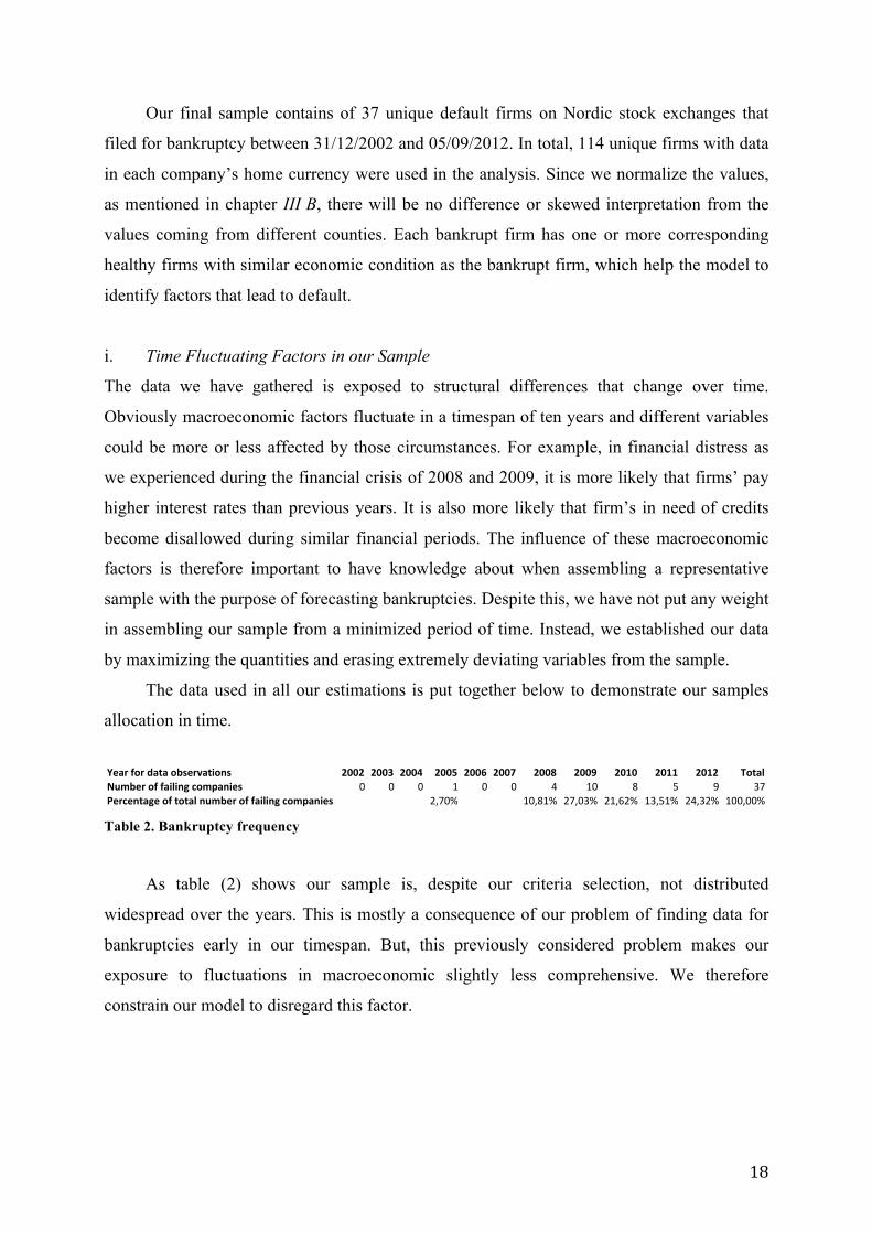
Our final sample contains of 37 unique default firms on Nordic stock exchanges that

filed for bankruptcy between 31/12/2002 and 05/09/2012. In total, 114 unique firms with data

in each company’s home currency were used in the analysis. Since we normalize the values,

as mentioned in chapter III B, there will be no difference or skewed interpretation from the

values coming from different counties. Each bankrupt firm has one or more corresponding

healthy firms with similar economic condition as the bankrupt firm, which help the model to

identify factors that lead to default.

i. Time Fluctuating Factors in our Sample

The data we have gathered is exposed to structural differences that change over time.

Obviously macroeconomic factors fluctuate in a timespan of ten years and different variables

could be more or less affected by those circumstances. For example, in financial distress as

we experienced during the financial crisis of 2008 and 2009, it is more likely that firms’ pay

higher interest rates than previous years. It is also more likely that firm’s in need of credits

become disallowed during similar financial periods. The influence of these macroeconomic

factors is therefore important to have knowledge about when assembling a representative

sample with the purpose of forecasting bankruptcies. Despite this, we have not put any weight

in assembling our sample from a minimized period of time. Instead, we established our data

by maximizing the quantities and erasing extremely deviating variables from the sample.

The data used in all our estimations is put together below to demonstrate our samples

allocation in time.

Table 2. Bankruptcy frequency

As table (2) shows our sample is, despite our criteria selection, not distributed

widespread over the years. This is mostly a consequence of our problem of finding data for

bankruptcies early in our timespan. But, this previously considered problem makes our

exposure to fluctuations in macroeconomic slightly less comprehensive. We therefore

constrain our model to disregard this factor.

Year%for%data%observations 2002 2003 2004 2005 2006 2007 2008 2009 2010 2011 2012 TotalNumber%of%failing%companies 0 0 0 1 0 0 4 10 8 5 9 37Percentage%of%total%number%of%failing%companies 2,70% 10,81% 27,03% 21,62% 13,51% 24,32% 100,00%

19

ii. Analysis of the Country Selection

Each year the World Bank put together a index based on empirical data measuring the “ease

of doing business” in different countries. The index is meant to describe how healthy the

business environment is when operating and starting a firm. This data is unfortunately based

on larger companies than the ones used in our model. Still, the data presents a description of

how equivalent the business climate is in different countries. As we gathered data from

Sweden, Norway, and Denmark the ranking between these countries are interesting to

analyse. In 2012, Sweden was ranked thirteenth, Denmark fifth and Norway sixth on the

assembled rating of all analysed countries. This is pleasant for us, as it strengthens our

primary assumption that these three countries are plausible in the explanatory power of a

bankruptcy in a regression.

Differences among the countries are nevertheless inevitable. In the index one of the

variables represent the ability of resolving insolvency where Norway is ranked as number two

and Sweden ranked eighteenth. Yet, due to limitations in our essay, we assume that the

parameters have an equally important contribution to the forecasting of bankruptcy regardless

of country in our model.

It would have been interesting for us to analyse how the index corresponds to the mean

Z-score of each country in our model. However, since our sample from both Norway and

Denmark is significant smaller than Sweden analysis is not possible. (World Bank and IFC

(2012))

iii. Logit Transformation

As we transform all Z-values from each company into probability parameters using the logit

model, our data through one to five years ahead of failure shapes as follows in figure (2). In

theory this curve is supposed to look like figure (1), which gives the best interpretation and

shows how the dataset cover both bankruptcies and non-bankruptcies. The transformed Z-

values also tell us how well the model explains failures and survivors. A misshaped S-curve

indicates a defective model.

20

Figure 2. Our transformed Z-values into logit probabilities

It is well defined in the graphs in figure (2) that the probabilities lay within the

restriction, 0 < (Pr 𝑌 = 1 ) < 1. The most important understanding of the S-curve is that the

larger value of the risk variable Zi the higher is the probability of default, which is exactly

how the plotted data in figure (2) works. The data testing values two years prior to bankruptcy

seems to have an S-curve that looks like the optimal one (figure (1)).

The intuitional interpretation of the diagram is as follows: the probability parameter is

represented on the Y-axis and the Z-value on the X-axis. When a company have a Zi value

that represents 0,5 on the Y-axis, the probability of default is fifty-fifty and the larger the Zi

value gets the higher the probability of default will be and vice verse. Again, the S-curve with

data two years prior to the event of bankruptcy have the best representation of both default

and non-default companies. We therefore suspect that our model can predict and categorize

bankruptcies and surviving companies best two years prior to the actual failure. But further

tests on the data are necessary.

B. Test for Misspecification

This sub-section tests the properties of our model.

i. Test of the Model’s Accuracy

First of all, we tested if our model could properly explain business defaults through a chi-

squared test. In order to decide how many years back the model could explain and predict

company defaults we ran the data through five tests, where each test represented one to five

years prior failure.

21

The first test, one year prior failure, is represented by 66 companies where 14 of them

went bankrupt and 52 survived. Since firms that are on the edge of bankruptcy normally show

signs of failure, a high score of accuracy is expected.

Table 3. One year prior default – type I, type II errors and chi-squared

As shown in the matrix above (table (3)) the model is accurate when classifying the

sample one year prior failure. A type II error is shown only as 9,6 per cent and a type I error

as 28,6 per cent. The chi-squared test on the sample presents a p-value, 0,0000009643, which

confirms the model with significance. The output from the results is promising, but not

enough to be convinced that our model can classify failures and surviving firms. Also, the

sample in this test consists of 52 surviving firms and only 14 bankruptcies. We must therefore

do further research.

The observations two years prior bankruptcy is our largest sample containing 82 firms

where we have 30 bankruptcies. The result is not as accurate as when modelling data one year

prior, but 70 per cent correct observations for bankruptcies profits the model and is

acknowledging evidence. The model does not only with significance classify failures

correctly but also surviving firms with 80,8 per cent accuracy.

Table 4. Two years prior default – type I, type II errors and chi-squared

Bankrupt Non+Bankrupt TOTBankrupt 10 4 14

Non+Bankrupt 5 47 52TOT 15 51 66

Number)Correct

Per)cent)Correct

Per)cent)Error n

Type)I 10 0,714 0,286 14Type)II 47 0,904 0,096 52Total 57 0,864 0,136 66 Chi8squared,)p 9.643E+07

Model

Actual



Number)Correct

Per)cent)Correct

Per)cent)Error n

Type)I 21 0,700 0,300 30Type)II 42 0,808 0,192 52Total 63 0,768 0,232 82 Chi8squared,)p 4.954E+06

Model

Actual

22

As seen in table (4) the chi-squared test of the model gives an output p-value of,

0,000004954, meaning it is significant on a 99 per cent level. Hence, the test is accurate two

years prior to the event of failure. Data tested two years after the event of failure gives a 30

per cent chance of a type I error and 19,2 per cent for a type II error, which is impressively

small and confirms our model. Even though the model is accurate two years prior bankruptcy

it is necessary to apply additional tests.

Our third test includes a total of 80 companies where 27 are failures. Since the model

have limitations we predict it not to be as accurate as it is two years prior. As shown in the

matrix in table (5) a type II error is present 43,4 per cent and a type I error 29,6 per cent. Even

though the chi-squared test’s p-value is higher than before, the test is still significant with a

level of 0,022.

Table 5. Three years prior default – type I, type II errors and chi-squared

In conclusion with table (5) the model cannot accurately categorize the groups, and the

interpretation becomes less clear.

When testing data four years prior bankruptcy, the test is not significant according to the

chi-squared p-value. The sample contains 68 firms where 23 have gone bankrupt.

Table 6. Four years prior default – type I, type II errors and chi-squared



Number)Correct

Per)cent)Correct

Per)cent)Error n

Type)I 19 0,704 0,296 27Type)II 30 0,566 0,434 53Total 49 0,613 0,388 80 Chi8squared,)p 0,022

Model

Actual



Number)Correct

Per)cent)Correct

Per)cent)Error n


Model

Actual

23

The model has a type I error 65,2 per cent, which is more like a guessing game rather

than a bankruptcy prediction model.

Since our sample five years prior to the event of bankruptcy only contains of 39

observations it does, according to Davidson and MacKinnon, not include enough information

in order to draw conclusions from the regression. Interestingly, our model estimates with 71,4

per cent accuracy the bankrupt group but as mentioned, it is impossible to make any

interpretation.

We generalize three, four, and five years prior bankruptcy as long-range predictive data,

as Altman (1968) does in his article of the Z-score model. This is done since the model’s

effectiveness decreases as the years increase from the event of bankruptcy. As a result of

tables (3-6) and the discussion above it is accurate and significant to forecast business failure

two years prior the bankruptcy event. The following years substantially decrease the chance

for our model to predict and correctly categorize failing or non-failing companies.

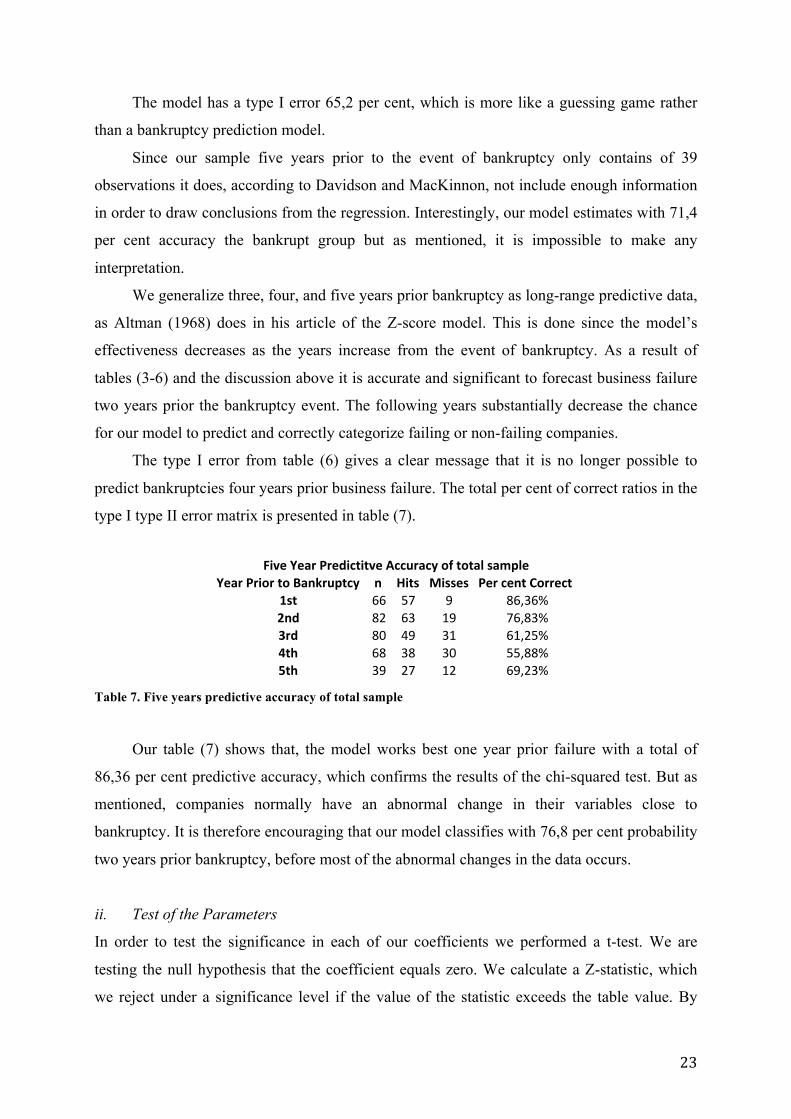
The type I error from table (6) gives a clear message that it is no longer possible to

predict bankruptcies four years prior business failure. The total per cent of correct ratios in the

type I type II error matrix is presented in table (7).

Table 7. Five years predictive accuracy of total sample

Our table (7) shows that, the model works best one year prior failure with a total of

86,36 per cent predictive accuracy, which confirms the results of the chi-squared test. But as

mentioned, companies normally have an abnormal change in their variables close to

bankruptcy. It is therefore encouraging that our model classifies with 76,8 per cent probability

two years prior bankruptcy, before most of the abnormal changes in the data occurs.

ii. Test of the Parameters

In order to test the significance in each of our coefficients we performed a t-test. We are

testing the null hypothesis that the coefficient equals zero. We calculate a Z-statistic, which

we reject under a significance level if the value of the statistic exceeds the table value. By

Year%Prior%to%Bankruptcy n Hits Misses Per%cent%Correct%1st 66 57 9 86,36%2nd 82 63 19 76,83%3rd 80 49 31 61,25%4th 68 38 30 55,88%5th 39 27 12 69,23%

Five%Year%Predictitve%Accuracy%of%total%sample

24

rejecting the null hypothesis the tested coefficient have significance in our model. The test is

executed on all our regressions from five years prior to bankruptcy until one year before with

different confidence intervals. By investigating this on our regressions we can draw

conclusions under which confidence interval our coefficients are significant. We can also see

how the significance in each coefficient fluctuates compared to the year prior to bankruptcy

and tell if there are any interesting differences.

Below you find our five hypothesis tests on the significance of the five coefficients

included in our model each year prior to bankruptcy. Important to notice is that by looking at

the p-values in table (8) it is possible to tell whether we can reject the null hypothesis or not.

It is possible to use different approaches regarding the level of accuracy. If the p-value

exceeds for example 0,05, it is more than a 5 per cent probability that the null hypothesis is

true (Dougherty (2011)). The test is generated using EViews.

Table 8. One to five years prior bankruptcy – test of parameters

With regards to the differences in the number of observations among the tests, the

significances should be interpreted with caution. For example, the last five years prior to

bankruptcy prediction do not have enough observations to draw any subjective conclusions

regarding the significances.

In line with the conclusions from the chi-squared test, the strongest predicting power for

bankruptcy is given one and two years prior the event of bankruptcy. These two models are

thus the most interesting to evaluate. Altman chose to focus his analyse on the two years prior

to bankruptcy as his one year prior to bankruptcy did not give unbiased estimates. Therefore

we have also chosen to analyse our forecasting model two years prior to bankruptcy.

Variable Coefficient. Prob. Coefficient. Prob. Coefficient. Prob. Coefficient. Prob. Coefficient. Prob.X1 0,036 0,249 0,026 0,020 0,013 0,240 0,000 0,996 0,018 0,589X2 0,043 0,111 0,022 0,165 +0,002 0,919 0,008 0,704 0,079 0,190X3 +0,246 0,011 +0,119 0,000 +0,043 0,055 +0,072 0,083 +0,588 0,048X4 +0,039 0,024 +0,011 0,008 +0,006 0,176 +0,011 0,003 +0,024 0,119X5 +1,397 0,222 +0,350 0,461 0,394 0,235 0,336 0,437 5,759 0,078

Obs.with.Dep.=.0Obs.with.Dep.=.1

5.Year.PriorTest.of.Parameters

52------------------------------------------14

52-----------------------------------------30

53---------------------------------------27-

45---------------------------------------23-

32-----------------------------------------7-

1.Year.Prior 2.Year.Prior 3.Year.Prior 4.Year.Prior

25

C. Our Bankruptcy Prediction Model

Henceforth in this thesis, we refer to the estimations based on the data from two years prior to

bankruptcy, when we analyse the results. When we discuss Altman’s model we also refer to

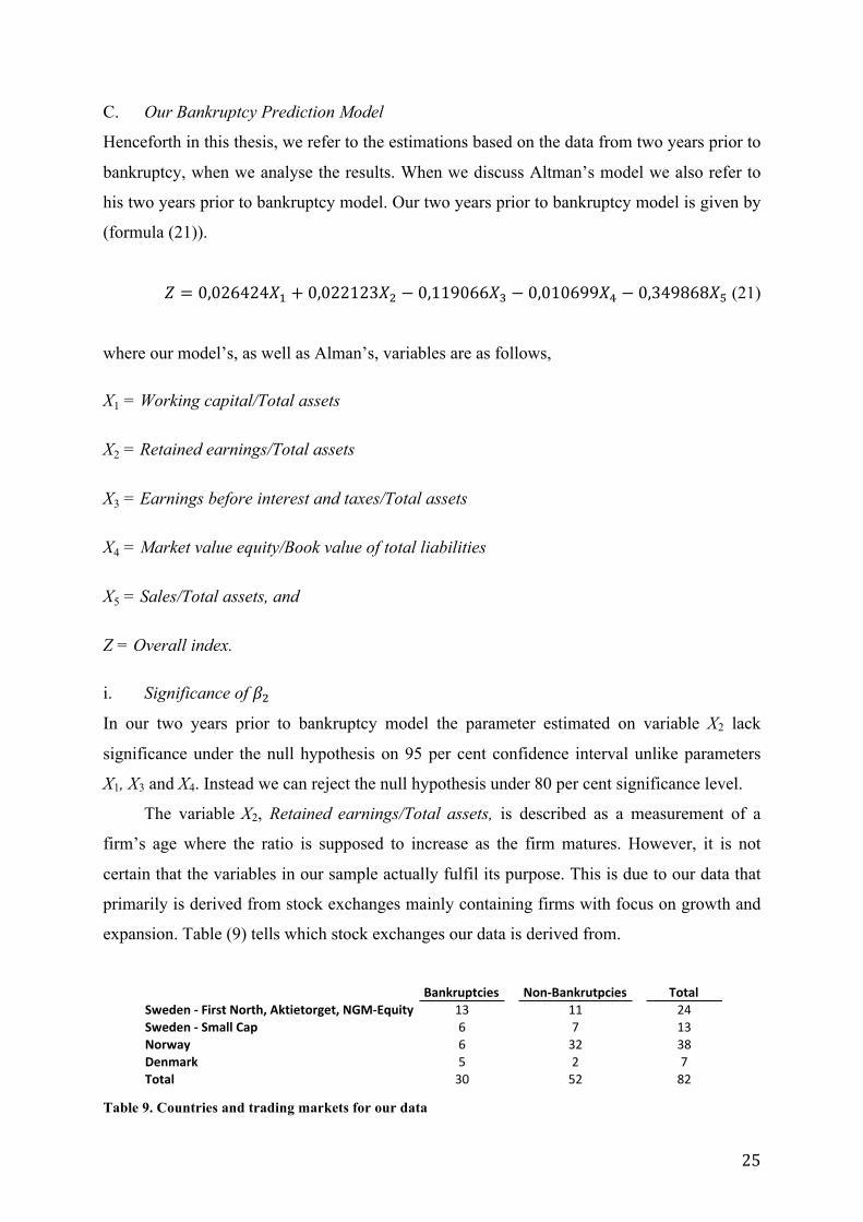
his two years prior to bankruptcy model. Our two years prior to bankruptcy model is given by

(formula (21)).

𝑍 = 0,026424𝑋! + 0,022123𝑋! − 0,119066𝑋! − 0,010699𝑋! − 0,349868𝑋! (21)

where our model’s, as well as Alman’s, variables are as follows,

X1 = Working capital/Total assets

X2 = Retained earnings/Total assets

X3 = Earnings before interest and taxes/Total assets

X4 = Market value equity/Book value of total liabilities

X5 = Sales/Total assets, and

Z = Overall index.

i. Significance of 𝛽!

In our two years prior to bankruptcy model the parameter estimated on variable X2 lack

significance under the null hypothesis on 95 per cent confidence interval unlike parameters

X1, X3 and X4. Instead we can reject the null hypothesis under 80 per cent significance level.

The variable X2, Retained earnings/Total assets, is described as a measurement of a

firm’s age where the ratio is supposed to increase as the firm matures. However, it is not

certain that the variables in our sample actually fulfil its purpose. This is due to our data that

primarily is derived from stock exchanges mainly containing firms with focus on growth and

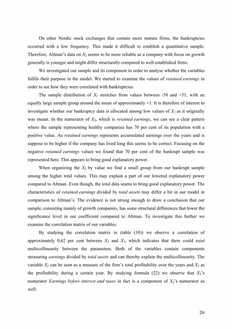
expansion. Table (9) tells which stock exchanges our data is derived from.

Table 9. Countries and trading markets for our data

Bankruptcies Non/Bankrutpcies TotalSweden5/5First5North,5Aktietorget,5NGM/Equity 13 11 24Sweden5/5Small5Cap 6 7 13Norway 6 32 38Denmark 5 2 7Total 30 52 82

26

On other Nordic stock exchanges that contain more mature firms, the bankruptcies

occurred with a low frequency. This made it difficult to establish a quantitative sample.

Therefore, Altman’s data on X2 seems to be more reliable as a company with focus on growth

generally is younger and might differ structurally compared to well-established firms.

We investigated our sample and its component in order to analyse whether the variables

fulfils their purpose in the model. We started to examine the values of retained earnings in

order to see how they were correlated with bankruptcies.

The sample distribution of X2 stretches from values between -58 and +51, with an

equally large sample group around the mean of approximately +1. It is therefore of interest to

investigate whether our bankruptcy data is allocated among low values of X2 as it originally

was meant. In the numerator of X2, which is retained earnings, we can see a clear pattern

where the sample representing healthy companies has 70 per cent of its population with a

positive value. As retained earnings represents accumulated earnings over the years and is

suppose to be higher if the company has lived long this seems to be correct. Focusing on the

negative retained earnings values we found that 70 per cent of the bankrupt sample was

represented here. This appears to bring good explanatory power.

When organizing the X2 by value we find a small group from our bankrupt sample

among the higher total values. This may explain a part of our lowered explanatory power

compared to Altman. Even though, the total data seams to bring good explanatory power. The

characteristics of retained earnings divided by total assets may differ a bit in our model in

comparison to Altman’s. The evidence is not strong enough to draw a conclusion that our

sample, consisting mainly of growth companies, has some structural differences that lower the

significance level in our coefficient compared to Altman. To investigate this further we

examine the correlation matrix of our variables.

By studying the correlation matrix in (table (10)) we observe a correlation of

approximately 0,62 per cent between X2 and X3, which indicates that there could exist

multicollinearity between the parameters. Both of the variables contain components

measuring earnings divided by total assets and can thereby explain the multicollinearity. The

variable X2 can be seen as a measure of the firm’s total profitability over the years and X3 as

the profitability during a certain year. By studying formula (22) we observe that X3’s

numerator Earnings before interest and taxes in fact is a component of X2’s numerator as

well.

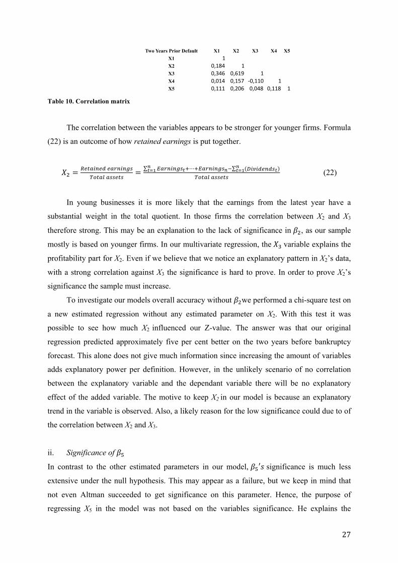
27

Table 10. Correlation matrix

The correlation between the variables appears to be stronger for younger firms. Formula

(22) is an outcome of how retained earnings is put together.

𝑋! =!"#$%&"' !"#$%$&'

!"#$% !""#$"= !"#$%$&'!!⋯!!"#$%$&'!! (!"#"$%&$'!)!

!!!!!!!

!"#$% !""#$" (22)

In young businesses it is more likely that the earnings from the latest year have a

substantial weight in the total quotient. In those firms the correlation between X2 and X3

therefore strong. This may be an explanation to the lack of significance in 𝛽!, as our sample

mostly is based on younger firms. In our multivariate regression, the 𝑋! variable explains the

profitability part for X2. Even if we believe that we notice an explanatory pattern in X2’s data,

with a strong correlation against X3 the significance is hard to prove. In order to prove X2’s

significance the sample must increase.

To investigate our models overall accuracy without 𝛽!we performed a chi-square test on

a new estimated regression without any estimated parameter on X2. With this test it was

possible to see how much X2 influenced our Z-value. The answer was that our original

regression predicted approximately five per cent better on the two years before bankruptcy

forecast. This alone does not give much information since increasing the amount of variables

adds explanatory power per definition. However, in the unlikely scenario of no correlation

between the explanatory variable and the dependant variable there will be no explanatory

effect of the added variable. The motive to keep X2 in our model is because an explanatory

trend in the variable is observed. Also, a likely reason for the low significance could due to of

the correlation between X2 and X3.

ii. Significance of 𝛽!

In contrast to the other estimated parameters in our model, 𝛽!′𝑠 significance is much less

extensive under the null hypothesis. This may appear as a failure, but we keep in mind that

not even Altman succeeded to get significance on this parameter. Hence, the purpose of

regressing X5 in the model was not based on the variables significance. He explains the

Two Years Prior Default X1 X2 X3 X4 X5X1 1X2 0,184 1X3 0,346 0,619 1X4 0,014 0,157 +0,110 1X5 0,111 0,206 0,048 0,118 1

28

insignificance as an effect of the multivariate regression where the other variables erase the

importance of X5.

Altman (1968) explained this as “Because of its unique relation to other variables in

the model, the Sales/Total assets ratio ranks second in its contribution to the overall

discriminating ability of the model”.2 Altman refers to an outcome of the high negative

correlation he found between X3 and X5 in the bankrupt group.

When we compare our correlations with Altman’s we did not find such a relationship.

Altman got a (-0,78) correlation between X3 and X5 while we received a correlation of

approximately (+0,05) (table (13)). Because of the low correlation this doesn’t appear to be a

preferable explanation to the lack of significance in X5 that we’ve received in our model.

To figure out what could cause the insignificance we examined our sample of X5. By

sorting the different observations according to size we examine whether we can observe a

pattern in the distribution. In line with our lack of significance in 𝛽!, a pattern is hard to

distinguish. This tells us that the sale rate in our data does not have any explanatory power.

The explanation may be consequences of some troubled companies practicing massive sales

in order to solve liquidity problems. These firms do therefore not break-even, examining only

their sales we disregard that the products may be sold even though making losses. The reason

to some of the high sales ratios among the bankrupt group might be found here. The

uncorrelated pattern between the dependant variable and our X5 variable could be a result of

how some firm’s solve their liquidity problems through sales and others may not have that as

an option.

iii. Marginal Effects

The marginal effect is calculated through the partial derivative of Xi. Because variables X1 to

X4 in our model are written as whole percentages, in comparison to X5, the marginal effects

among X1-X4 and X5 will differ. In order to make the marginal effect comparable we transform

them into the same unit. A unit increase for variable X1- X4 is 100 times larger than an equally

large unit change for variable X5. Therefore, we multiply the margin effect on the X1- X4

variables with 100. Our marginal effects are as follows in table (11).

2 Altman, 1968

29

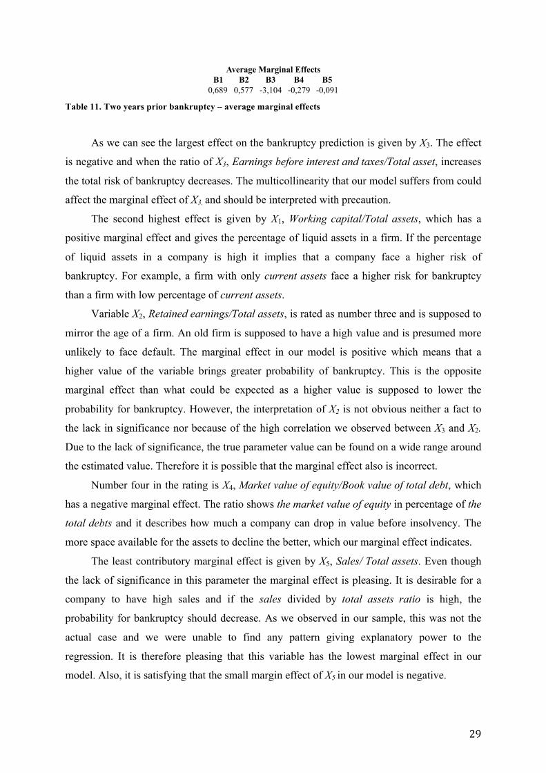
Table 11. Two years prior bankruptcy – average marginal effects

As we can see the largest effect on the bankruptcy prediction is given by X3. The effect

is negative and when the ratio of X3, Earnings before interest and taxes/Total asset, increases

the total risk of bankruptcy decreases. The multicollinearity that our model suffers from could

affect the marginal effect of X3, and should be interpreted with precaution.

The second highest effect is given by X1, Working capital/Total assets, which has a

positive marginal effect and gives the percentage of liquid assets in a firm. If the percentage

of liquid assets in a company is high it implies that a company face a higher risk of

bankruptcy. For example, a firm with only current assets face a higher risk for bankruptcy

than a firm with low percentage of current assets.

Variable X2, Retained earnings/Total assets, is rated as number three and is supposed to

mirror the age of a firm. An old firm is supposed to have a high value and is presumed more

unlikely to face default. The marginal effect in our model is positive which means that a

higher value of the variable brings greater probability of bankruptcy. This is the opposite

marginal effect than what could be expected as a higher value is supposed to lower the

probability for bankruptcy. However, the interpretation of X2 is not obvious neither a fact to

the lack in significance nor because of the high correlation we observed between X3 and X2.

Due to the lack of significance, the true parameter value can be found on a wide range around

the estimated value. Therefore it is possible that the marginal effect also is incorrect.

Number four in the rating is X4, Market value of equity/Book value of total debt, which

has a negative marginal effect. The ratio shows the market value of equity in percentage of the

total debts and it describes how much a company can drop in value before insolvency. The

more space available for the assets to decline the better, which our marginal effect indicates.

The least contributory marginal effect is given by X5, Sales/ Total assets. Even though

the lack of significance in this parameter the marginal effect is pleasing. It is desirable for a

company to have high sales and if the sales divided by total assets ratio is high, the

probability for bankruptcy should decrease. As we observed in our sample, this was not the

actual case and we were unable to find any pattern giving explanatory power to the

regression. It is therefore pleasing that this variable has the lowest marginal effect in our

model. Also, it is satisfying that the small margin effect of X5 in our model is negative.

B1 B2 B3 B4 B50,689 0,577 -3,104 -0,279 -0,091

Average Marginal Effects

30

D. Comparison to Altman’s marginal effects

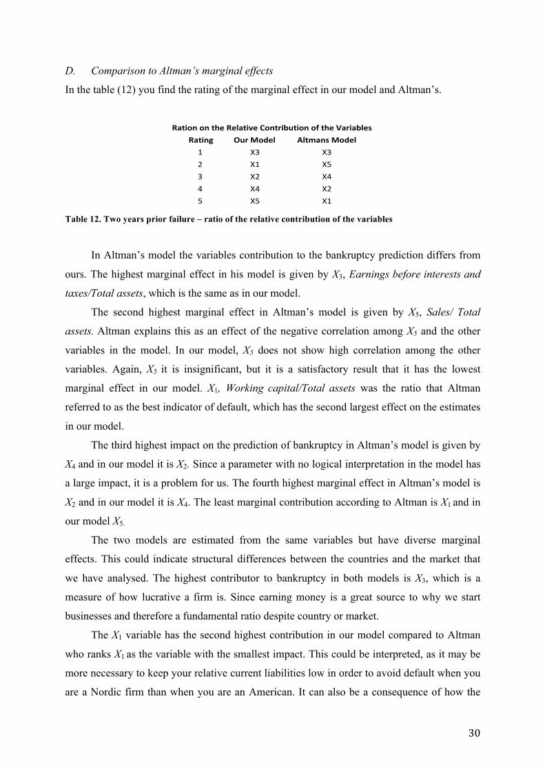
In the table (12) you find the rating of the marginal effect in our model and Altman’s.

Table 12. Two years prior failure – ratio of the relative contribution of the variables

In Altman’s model the variables contribution to the bankruptcy prediction differs from

ours. The highest marginal effect in his model is given by X3, Earnings before interests and

taxes/Total assets, which is the same as in our model.

The second highest marginal effect in Altman’s model is given by X5, Sales/ Total

assets. Altman explains this as an effect of the negative correlation among X5 and the other

variables in the model. In our model, X5 does not show high correlation among the other

variables. Again, X5 it is insignificant, but it is a satisfactory result that it has the lowest

marginal effect in our model. X1, Working capital/Total assets was the ratio that Altman

referred to as the best indicator of default, which has the second largest effect on the estimates

in our model.

The third highest impact on the prediction of bankruptcy in Altman’s model is given by

X4 and in our model it is X2. Since a parameter with no logical interpretation in the model has

a large impact, it is a problem for us. The fourth highest marginal effect in Altman’s model is

X2 and in our model it is X4. The least marginal contribution according to Altman is X1 and in

our model X5.

The two models are estimated from the same variables but have diverse marginal

effects. This could indicate structural differences between the countries and the market that

we have analysed. The highest contributor to bankruptcy in both models is X3, which is a

measure of how lucrative a firm is. Since earning money is a great source to why we start

businesses and therefore a fundamental ratio despite country or market.

The X1 variable has the second highest contribution in our model compared to Altman

who ranks X1 as the variable with the smallest impact. This could be interpreted, as it may be

more necessary to keep your relative current liabilities low in order to avoid default when you

are a Nordic firm than when you are an American. It can also be a consequence of how the

Rating Our*Model Altmans*Model1 X3 X32 X1 X53 X2 X44 X4 X25 X5 X1

Ration*on*the*Relative*Contribution*of*the*Variables

31

bankruptcy rules have changed during the years as Altman’s firms went bankrupt during the

1960s. Further differences are small among the rating of marginal effects, which make an

analysis hard to perform.

i. Chi-Squared Test of Altman’s Z-score Model

Finally, we tested Altman’s original Z-score model (formula (1)) against ours (formula (21))

in order to be sure that our estimated beta values can categorize bankruptcies and surviving

Nordic firms better than Altmans’. Since our earlier tests have showed that our model is best

two years prior the event of bankruptcy, the input for Xi was therefore the same as when we

made the test for our model. But, instead of using our estimated beta values Altman’s beta

values were used. The test was preformed through a chi-squared test, where we found out

how accurate Altmans’ classification is compared to ours.

Table 13. Two years prior default with Altman’s beta – type I, type II errors and chi-squared

When having the same input, Xi, two years prior default but with Altman’s beta values

the chi-squared p value in table (13) indicates that that the model is not significant and cannot

be used. This is strengthen by the type II error percentage error, 73,1 per cent. In other words,

our model predicts bankruptcies and categorizes non-bankruptcies on listed Nordic firms

better than Altman’s Z-score model does two years prior the event of default.

VI. Conclusion

With regards to the uncertain economical environment and the following effects such as

bankruptcies and high credit risks, it has gained importance for a precise default

measurement. We estimated our own bankruptcy prediction model based upon the variables

in Altman’s Z-score model and tested it on listed Nordic firms. We used a logit binary model

that gave us a Z-score, which measured the probability of default and non-default.



Number)Correct

Per)cent)Correct

Per)cent)Error n


Actual

32

Our sample contains of 114 unique firms where 37 of them went bankrupt between

31/12/2002 and 05/09/2012. We have used companies from Sweden, Norway, and Denmark

with normalized data to clean the differences among local currencies. We studied how

accurate our model could categorize these companies as either bankrupt or surviving.

We found that our model works best two years prior the event of bankruptcy and can

categorize defaults and non-defaults, on NGM-equity, Aktietorget, First North, and Small

Cap, with 76,8 per cent accuracy. When comparing our model to Altman’s Z-score model we

found that ours can categorize defaults and non-defaults better. With the favourable results of

our model, it could be implemented in the loan application processes in order to make more

confident and fair decisions regarding to accept loans or not.

Foremost, we have two key questions regarding our research data.

1) Did the amount of data delimitate our thesis and could our model become more

accurate with an extension of the collected data?

2) Where the parameters we used the best in order to minimize the mistakes in our

estimated bankruptcy prediction model?

We could probably have improved our estimation with a larger sample of bankrupt

firms. The fact that our data was derived from mainly growth firms was probably the reason

for lack of significance in 𝛽! as younger firms suffered from multicolinearity between 𝑋! and

X3. Financial ratios earlier than 2006 was inadequate and therefore our bankrupt sample are

clustered from 2007-2012. An archive with more comprehensive data from older companies

may therefore increase the sample and improve our model. On the other hand, a more

widespread timespan of data may expose our model to structural changes caused by

fluctuations in the macroeconomic environment that may harm our estimation. Since we

perceived our model to work best two years prior to the event of default, an extension of the

timespan would therefore not have gained any positive effect on our results. Also, as the years

increase after two years prior bankruptcy, the number of correct hits in the model decreases.

This is associated with our models increased incapability to differentiate between

bankruptcies and surviving firms over longer time spans.

Furthermore, increasing our sample to Finnish companies may have improved the

model without breaking our initial purpose of creating a bankruptcy prediction model for

Nordic firms. Due to language and time limitations the data from Finnish firms was very hard

to collect.

Another delimitation was our choice of variables. There are many interesting financial

ratios that would have explanatory power to a bankruptcy. We chose Altman’s variables as

33

delimitation despite the fact that he developed the model 1968. We believe the general factors

describing bankruptcy are gathered in the model and therefore we chose to delimitate our

estimation to those variables.

A broader and larger dataset and an increased amount of default companies would

probably improve our model and, as a result of that, improve the models accuracy. An

extension of the number of variables used would also give a clearer picture of a company’s

economical situation and improve our model. We suggest this to be subject for further

research.

34

References

Al-Rawi, K., Kiani, R., and Vedd, R. R., 2008, The use of Altman Equation For Bankruptcy

Prediction In An Industrial Firm (Case Study), International Business & Economics

Research Journal, Vol. 7.

Altman, E. I., 1968, Financial Ratios, Discriminant Analysis and the Prediction of Corporate

Bankruptcy, The Journal of FINANCE, Vol. XXIII.

Altman, E. I., Haldeman, R., and Narayanan, P., 1977, Zeta Analysis: A New Model to

Identify Bankruptcy Risk of Corporations, Journal of Banking & Finance, Vol. 1.

Chernoff, H., and Lehmann E. L., 1954, The Annuals of Mathematical Statistics, Institute of

Mathematical Statistics, Vol. 25.

Cohen, J., Cohen, P., West, S. G., and, Aiken L. S., 2003, Applied Multiple

Regression/Correlation Analysis for the Behavioral Sciences, Taylor & Francis Group,

Vol. 3.

Davidsson, R., and MacKinnon, J. G., 1982, Convenient Specification Test for Logit and

Probit Models, Journal of Econometrics, Vol. 25.

Dougherty, C., 2011, Introduction to Econometrics, Barnes & Noble, Vol. 4.

Farrar, D. E., Glauber, R., R., Multicollinearity in Regression Analysis: The Problem

Revisited, The Review of Economics and Statistics, Vol. 49.

Hole, A. R., 2006, Small-sample properties of tests for heteroscedasticity in the conditional

logit model, Economics Bulletin, Vol. 3.

Lennox, C., 1999, Identifying Failing Companies: A Revaluation of the Logit, Probit and DA

Approaches, Journal of Economics and Business, Vol. 51.

Mester, L., 1997, Whats the Point of Credit Scoring, Business Review.

Ohlson, J., 1980, Financial Ratios and the Probabilistic Prediction of Bankruptcy, Journal of

Accounting Research, Vol. 18.

Pampel, F. C., 2000, Logistic Regression – A Primer, SAGE Publications Inc., Vol. 132.

Schumway, T., 2001, Forecasting Bankruptcy More Accurately: A Simple Hazard Model, The

Journal of Business, Vol. 74.

The Reuters Glossary: A Dictionary of International Economic and Financial Terms by

Reuters Staff, 1989, Longman Publishing Group, Vol. 19.

Verbeek, M., 2012, A Guide to Modern Econometrics, Barnes & Noble, Vol. 4.

Westerlund, J., 2005, Introduktion till Ekonometri, Studentlitteratur AB, Vol. 1.

35

i. Other References

Business Dictionary, Search phrase: retained earnings, www.businessdictionary.com.

Standard & Poor’s ratings credits definitions, www.standardandpoors.com.

The World Bank, Economy Rankings, www.doingbusiness.org.

variables important for bankruptcy prediction - a...

Documents