variability of variograms and spatial estimates due to

Geoderwza, 62 (1994) 165-182 Elsevier Science B.V., Amsterdam

165

Variability of variograms and spatial estimates due to soil sampling: a case study

C . Gascuel-Odouxa,b and P. Boivinb aInstitut National de la Recherche Agronomique, Science du Sol, 65 route de Saint-Brieuc,

35042 Rennes cedex, France bORSTOM, l’Institut Français de Recherche Scientifique pour le DPveloppement en Coopèration,

Pèdologie, B.P. 1386, Dakar, SénPgal (Received July 15, 1992; accepted after revision February 24, 1993)

ABSTRACT

Measuring of electromagnetic soil conductivity (EMC) is used to follow the temporal evolution of soil salinity, because it is a rapid technique with a portable instrument. A test site of 1.2 km by 2.4 km is selected as a reference. The suitability of sampling schemes for monitoring soil salinity during the first years of irrigation is studied. An initial sampling consists of 17 rows and 33 columns of observation points 75 m apart, i.e. 561 data points, regularly spaced on 288 ha; it allows to determine the “actual variogram” of EMC on this site. This structure is complex, as is often the case in nature, with alternating strongly and weakly salted areas, due to small creeks across the site. The sample size required to get accurate estimates of soil salinity and to follow temporal changes is assessed by sub- sampling the data set.

Simulation by repeated sub-sampling is preferred because of the complexity of the data structure. Five series of 20 sub-samples are randomly taken from the initial sample, with size 50, 75, 100, 150 and 200 data points, respectively. For each sample size, the analysis consists in computing the mean squared error of the 20 sub-sample variograms relative to the “actual sample variogram”’, and similarly for the fitted models. Confidence limits for the theoretical variogram were directly estimated from the 20 fitted models. Finally, the effect of this uncertainty is studied by comparing kriged estimates with observed values.

The consistency of both experimental and fitted variograms increases with sample size. In this case, a choice of 150 data points appears to be consistent. Despite a larg$ variability in experimental variograms, the fitted models and the kriged estimates are not so different as could be expected.

INTRODUCTION

Estimation of the sample variogram and selection of an appropriate model for the theoretical variogram are essential steps in any geostatistical analysis. Kriging techniques are generally applied without any consideration on the uncertainty associated with estimating the theoretical variogram (Oliver and Webster, 199 1 ). Several sources of error may be considered: firstly, only one realization is generally available in nature and it is considered as representa- tive of all others; also, errors in the experimental variogram, due to sampling

0016-706 1/94/$07.00 O 1994 Elsevier Science B.V. All rights reserved. SSDZ O0 1 6-7 06 1 ( 9 3 ) E007 1-3

I O 1 O0 17062

Fonds Documentaire ORSTOM

c

I

166 $.

C. GASCUELODOUX AND P. BOIVIN

1

and measurement must be considered; secondly, errors may result from the choice of the model and estimation of the theoretical variogram. In the following, the term “variogram” will refer to the theoretical variogram; “sample variogram” refers to the experimental variogram.

Many investigations have studied variogram estimators (Davis and Borg- man, 1978,1982; Myers, 1985,199 1 ) and performed of how to improve their estimation. For instance, Russo ( 1984) and Warrick and Myers ( 1987) proposed a method to select an optimal sampling network; Cressie and Hawkins ( 1980) and Cressie ( 1984) introduced a method for robust estimation of a variogram; Unlü et al. (1990) compared several methods to fit a model to the sample variogram. Besides these improvements in geostatistical practices, the consistency of the sample variogram, which is the basis to determine the variogram, has also been investigated. The effect of sampling on the accur- racy of sample variograms is studied from independently generated random fields (Muñoz-Pardo, 1987; Russo and Jury; 1987,1988; Webster and Oliver, 1992) and from experimental data (Entz and Chang, 199 1 ; Van Meirvenne and Hofman, 199 1 ). More generally, Shafer and Varljen ( 1990) proposed a

about the consequences on models and estimates? The aim of this paper is to investigate the consequences of the uncertainty

introduced by the choice of a sampling scheme on sample variogram estimation and the following steps of a geostatistical study: fitting models, determining parameters such as nugget effect or autocorrelation distance, which as such are interesting aspects of the spatial structure, and kriging spatial estimates. As a matter of fact, a point of view would be that unsmoothed aspects of a sample variogram, due partly to the sampling effect, may be partly smoothed away by fitting a model, which is finally the one used in kriging. So it is necessary to examine the uncertainty at different steps of geostatistical analysis; not only at a single step such as the sample variogram estimation.

The practical purpose of this case study is to establish a reliable sampling strategy to detect temporal changes of soil salinity on test sites of 288 ha, selected as references to follow soil salinity during the first years of irrigation. These areas are located on different soil types. On each test site, a large initial sample is taken to enable optimization of subsequent sampling for temporal salinity evolution, Only one site is studied here.

More generally, chemical studies often show alternating rich and poor areas in the field. In these cases the effects of sampling should be carefully considered.

I

I

I jacknife method to establish confidence limits on sample variograms. But what !

I 1

MATERIAL AND METHODS

This study takes place in the middle part of the Senegal river valley where irrigation management for rice crops have been carried out despite some local

. ... -

. . " 1 . . . c,*,v>.

_._L .. , - Ad-*.:&- ' . ...- . . . . . . . - . . .

VARIABILITY OF VARIOGMMS AND SPATIAL ESTIMATES DUE TO SOIL SAMPLING 167

risks of soil salinisation. In this context, an early detection of a change in soil salinity allows adapting the agricultural practices. The valley is divided into successive basins with a few sedimentary depressions. The study site is located in one of these depressions and consists of Vertisols.

The variable of interest is an electromagnetic conductivity (EMC) measurement taken at the soil surface by a portable device (EM-38); it is well correlated (99%) with the soil bulk electrical conductivity measured at different depths (Rhoades and Convin, 1981). This technique is well adapted to follow soil salinity changes (Boivin et al., 1989).

The initial sampling consists of 17 rows and 33 columns of observation points 75 m apart, i.e. 561 data points regularly spaced on 288 ha. The EMC data range from O to 280 mS/m, with an average value of 88 mS/m, and a standard deviation of 69 mS/m. A chi-square goodness of fit test showed that the data may be assumed to have a log-normal distributiob (Fig. I ) , as is often the case with chemical data.

This intensive initial sampling allows to determine the structure of the variable of interest Z on this site, which will be considered as the theoretical structure. An estimate of the "actual sample variogram", denoted as ~ * ~ ( h / ) , is given by:

II where N ( h f ) is the number of pairs of points at each lag 1. The variogram appears to be complex, with alternating large and smalI val- i, I

ues

EO

60

s $40 e! U

20

O

(Fig. 2A) due to some small creeks across the

~ " ? ~ - - ~ ~ - - " , . . . - - . ¡ ~ - ~ l..._"..~̂ " "..I , _? ,,.. ~ , ~ . " - ~ - ~ _I_..._ .... ~ i... II......." ...... I .... ~ ................. 1 I

site, as it is often the

O 1 O0 200 300 400 Electromagnetic conductivity (mslm)

Fig. 1. Log-normal distribution fitted to the total data set of EMC measurements.

case

168

2- h

5 1.6-

U

u)

- m >

g 1.2- z O 5 0 . 8 . - 8 O

.- a c m .- ??i 0.4-

E I o.

(A)

+ + +

Raw A O" + 45" 0 90" X 135" + +

? 9

o x x x X O A +

A + x g A + x x

4

m > U X 135" w 1.2

ò 5 0.8

E 8

.- a I

c m 'C m

E O4 I

Distance (m) O 400 800 1200


Fig. 2. Raw and directional sample variogram for (A) the total data set (561 points); (B) without data located along creeks (400 points).

Distance (m) Fig. 3. EMC kriged map computed from the total data set (561 points).

VARIABILITY OF VARIOGRAMS AND SPATIAL ESTIMATES DUE TO SOIL SAMPLING 169

in this context. Removing the part of the data located along these creeks does not really change the spatial structure (Fig. 2B).

More generally, environmental fields in nature very often show particular features which make it impossible to deal with the sampling problem only by using simulations of random fields.

The model fitted on the “actual sample variogram” is considered as the “actual variogram”.

The kriged map, built from a linear plus a spherical model, confirms the heterogeneity of this spatial field, due to the presence of creeks (Fig. 3). De- spite this heterogeneity, the intrinsic hypothesis may be considered as locally valid according to continuous change in the major part of this field.

Sample variogram -

Because of the complexity of the data, a sub-sampling procedure is chosen to investigate the consistency of the sample variogram and spatial estimates. Five series of 20 sub-samples, with sample size 50,75, 100, 150 and 200 data points, respectively, are randomly taken from the initial sample. The sub- samples are taken independently from each other; so any results derived from them are stochastically independent, irrespective of the sampling fraction or the structure of the initial sample data (De Gruijter and Ter Braak, 1992). For each sub-sample, locations are randomly and independently selected. This choice simulates the most common procedure for which the sampling design is generally determined before any data collection, independent of the data distribution.

Sample variograms are computed from the 1 O0 sub-samples, according to:

15001 50data I Q 75data X B 5 1200- A 100data

a 150data x x c X 200data x x X x x x g 900- X

õ 600- x o O D D o o

5 A

2 b * ? * . e . o o . * . t f

O X Ll e X .-

G J D

o u âl (3 R

(u 0 3 0 0 - ’ x D n A A ~ A A A A A A A A ~

c U ~ , 4 9 ~ * * b f * : * ’ *

X

300 600 900 1200 Distance (m)

Fig. 4. Number of pairs of points per lag, averaged over 20 sub-samples, for each sample size: 50,75, 100, 150 and 200 points.

1’

i’

170 C. GASCUEL-ODOUX AND P. BOIVIN

where the indices Nand Kdenote the sample size and sub-sample, respectively. Sample variograms are all computed for a lag of 75 metres, which corre-

sponds to the mesh of the initial grid. The average distance hl per lag has been approximated by the central point in this lag in order to simplify calculations and allow comparisons. Root mean squared errors on this distance, 1.89,1.35, 0.99,0.64 and 0.37 m for the five sample sizes, respectively, can be neglected considering the lag value. Computation and fitting on sample variograms are limited to the first sixteen lags, Nlag i.e. 1200 my which is half the length of the field. For each sample size the number of pairs of points per lag increases to a distance of 700 m and then levels off (Fig. 4). From one sample size to the next larger one, the number of pairs of points per lag is approximately doubled.

The mean sample variogram of each sample size is: 1 20

Various measures of error in sub-sample variograms may be defined in ce- lation to the “actual sample variogram” rf (hl) . The following root mean squared errors are retained:

Equations (4) , (5) and (6) respectively represent: the deviation of an individual sub-sample variogram from the “actual sample variogram”, averaged over lags (eq. 4); the deviation of sub-sample variograms, averaged over lags and sub-samples, for a given sample size (es. 5); the deviation of the mean sample variogram for a given sample size, averaged over lags (eq. 6).

The results are also expressed in normalized values, the semivariance being divided by sub-sample variances.

Fitted variograms

Models are fitted by the simplex method (Chen et al., 1986). This method has the advantage to give results independent of the initial parameters, hence depending only on the data. It has been adapted here to the fitting of spatial

. _.- I


depending only on the data. It has been adapted here to the fitting of spatial structure models. Two fittings are realized: with or without taking into ac- count the number of pairs of points per lag in the sample variogram (Mc- Bratney and Webster, 1986). Two models are retained: (1 ) the model with the smallest MSE computed from model and sample variogram for three kinds of model: linear, spherical or linear plus spherical model; (2) a periodical component (Webster, 1985) is added if it improves the fitting, despite the fact that it is not an authorized model for two-dimensional fields. The idea is to examine if changing from a four- to a six-parameter model may better ac- count for the complexity of the data structure and if the accuracy on the estimated parameters of the model is improved.

The consistency of estimated parameters for each sample size is examined, according to the fitting procedure and type of model. At this step, as previ- ously, errors are measured by the RMSE of the models fitted on the sub-sample variograms and with respect to the “actual variogram”. A 95% confidence interval is calculated for each sample size.

Kriging estimates

The selected models and the data of each sub-sample are used to krige spa-

For each sample size, the RMSE, of the estimates Zi* is computed by com- tial estimates and estimated variances at the 56 1 points of the initial grid.

parison with the observations Zj:

where RMSEN is a measure of kriging error.

corresponding errors (Russo and Jury, 1987):

’

Similarly the RMRE, tests if the kriging variances are consistent with the

These two measures for kriging estimates may be defined analogously to eq. (4) for each individual sub-sample and denoted as RMSEAT,~ and RMRE,,,

y i 4 RESULTS

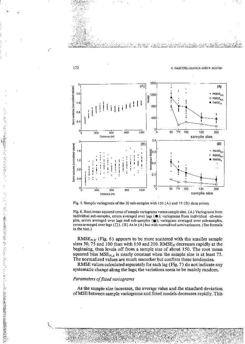
Sample variograms

k’& The 20 normalized sub-sample variograms, for sample size 50 and 150 are v 2 ’ i ; represented in Fig. 5. The former show far more scatter than the latter.

:.

J' , , .'.

172

300 600 900 120c 04 O

Distance (m)


* : 1200- RMSE,,,

cn 2 O RMSE,,, LT m RMSE,

800-

400- !

Oil 50 75 100 150 200 samde size

O O 300 600 900 1200

' RMSEN,KI

0 RMSE,,, RMSE,

n

50 75 100 150 200 Distance (m) sample size

Fig. 5. Sample variograms of the 20 sub-samples with 150 (A) and 75 (B) data points.

Fig. 6. Root mean squared error of sample variograms versus sample size. (A) Variograms from individual sub-samples, errors averaged over lags (O ); variograms 'from individual .ub-Sam- ples, errors averaged over lags and sub-samples (u); variogram averaged over sub-samples, errors averaged over lags ( O ). (B) As in (A) but with normalized semivariances. (See formula in the text.)

RMSEN,K (Fig. 6) appears to be more scattered with the smaller sample sizes 50,75 and 1 O0 than with 150 and 200. RMSEN decreases rapidly at the beginning, then levels off from a sample size of about 150. The root mean squared bias MSEN,A is nearly constant when the sample size is at least 75. The normalized values are much smoother but confirm these tendencies.

RMSE values calculated separately for each lag (Fig. 7) do not indicate any systematic change along the lags; the variations seem to be mainly random.

Parameters offitted variograms

As the sample size increases, the average value and the standard deviation of MSE between sample variograms and fitted models decreases rapidly. This

k, . .~

. . . .

1 -

VARIABILITY OF VARIOGRAMS AND SPATIAL ESTIMATES DUE TO SOIL SAMPLING

I I 4 100poinu I I I

1200- u v) z

800.-

400.-

0~ 900 1200 O 300 600

Distance (m)

+ 50points -D 150pointr (6) + 75 points d- 100ooinu

++ 200 painu

173

n w = 0.2-

z

0.1.-

300 600 900 1200 Distance (m)

Fig. 7. Root mean squared error of sample variograms versus disfance. (A) Original semivariances. (B) Normalized semivariances.

is illustrated in Fig. 8 for the simplest model, i.e. spherical plus linear component model. The structure is determined more and more accurately as the sample size increases because the sample variograms become smoother and differences between them become smaller.

Despite this better consistency of the models, according to the sample size, parameters of the fitted variograms do not seem to be determined more accurately for the three smaller sample sizes 50,75 and 100: the standard deviations of the nugget effect and, to a lesser extent, of slope, sill and range are quite similar, without any decrease. Results from normalized values do not differ anyway. However, average values of parameters are quite similar for the various sample sizes. Slope and sill seem to be slightly correlated.

Fitting with weighting variogram by the number of pairs does not really change average values and standard deviations of parameters.

Changing from a 4- to a 6-parameter model significantly reduces the MSE and their standard deviations (Fig. 9). However, this improvement must be compared to various other negative effects: the variability of the various pa-

:::::i 0.4-

0.2--

0-

-

normalized nugget effect

1 000-.

O slope

. . . . _ . . .

~.. e,. . .. ,, A'.... ~

174 C. GASCUEGODOUX AND P. BOIVIN

M.S.E. 11 600

range

0.6 '4 3000

2000 "t IT

0.4

0.6

0.4 i

ormalized sill 4 i P. sill

4 f ? o*:l

normalized slope

6E-4 t T 2E-4

o 60 76 100 160 o'SO '76 100 I60 200" fu sample sire g sample sire

Fig. 8. Parameters of a spherical plus a linear model, versus sample size: average value (a) and standard deviation for unweighted fitting; average value for weighted fitting (O ). Range is in metres. MSE mean squared error of fitted models from sample variograms, average over lags and sub-samples.


1

0.8

0.6

0.4

0.2

O

0.8

0.6

0.4

0.2

O

0.8

0.6

0.4

0.2

O

6E-4

4 E 4

2E-4

O

0.1

1200

1000

800

600

400

I 5 - 1 I - @

f -

normalized nugget effect

normalized sill

$8 i € 5

normalized slope

normalized amplitude

periodicit) T

T I

,I 1 II

$0 75 100 150 20d' fui sample size

range

2ooi nugget effect

3000

4000

2000

1 O00 I

I slop€ O

2 f- 1 4- o O amplitude

T

I l

0J'í50 75 100 150 200" full sample size

Fig. 9. Parameters of a spherical plus a linear and periodic component model, versus sample size: average value (m) and standard deviation for unweighted fitting; average value for weighted fitting (O). Range and periodicity are in metres. MSE: mean squared error of fitted models from sample variograms, average over lags and sub-samples.

. .

(A) - S*L ("p) -D. S+L (p) - S+L+P ("P) S+L+P (P) 1200

I '* c

'


900

600.-

300.

$

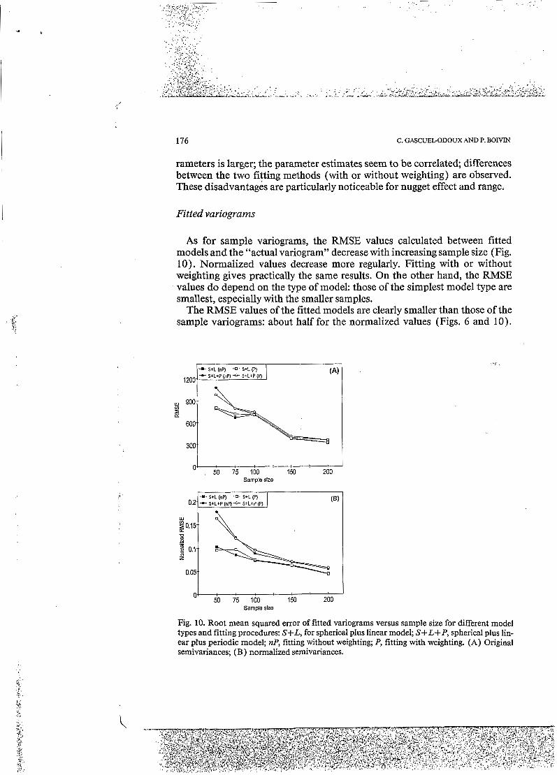
rameters is larger; the parameter estimates seem to be correlated; differences between the two fitting methods (with or without weighting) are observed. These disadvantages are particularly noticeable for nugget effect and range.

Fitted variograms

As for sample variograms, the RMSE values calculated between fitted models and the "actual variogram" decrease with increasing sample size (Fig. 10). Normalized values decrease more regularly. Fitting with or without weighting gives practically the same results. On the other hand, the RMSE values do depend on the type of model: those of the simplest model type are smallest, especially with the smaller samples.

The RMSE values of the fitted models are clearly smaller than those of the sample variograms: about half for the normalized values (Figs. 6 and 10).

o . 50 75 100 150 200 Sample size

(61 -œ- S+L (nP) -D S+L (P) 0.2 - S+L+P ("P) Q S+L+P (P)

~

150 200 o 50 75 100 Sample size

Fig. 10. Root mean squared error of fitted variograms versus sample size for different model types and fitting procedures: S+L, for spherical plus linear model; S+L+P, spherical plus linear plus periodic model; nP, fitting without weighting; P, fitting with weighting. (A) Original semivanances; (B ) normalized semivariances.

. _.- -


+ 50data U 150data (A) 1000

C 75 data * 200 dala

'O0/

300 600 900 1200 Distance (m)

G- 0.12

3 0.08 N

p 0.04

-C 75 data * 200 dala -C 75 data * 200 dala

I 300 600 900 1200

Distance (m)

Fig. 1 1. Root mean squared error of fitted variograms for a spheical plus linear model without weighting. (A) Original semivariances; (B ) normalized semivariances.

TABLE 1

Half-width of 95% confidence interval for a spherical plus linear model

Distance (m) Sample size

50 75 200

75 600 1200

280 334 360

255 238 364

127 121 179

The errors in the fitted models are largest near the autocorrelation distance and at the end of the variogram (Fig. 1 1 ); this applies particularly to the 4- parameter model.

Despite these errors, the 95% confidence interval appears to be narrow. It

i


i

is constant for nearly half distance (600 m), then increases by about 50% at 1200 m (Table 1 ). It doubles by reducing the sample size from 200 to 75.

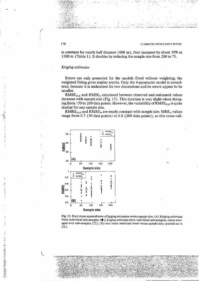
Kriging estimates

Errors are only presented for the models fitted without weighting; the weighted fitting gives similar results. Only the 4-parameter model is considered, because it is authorized for two dimensions and its errors appear to be smaller.

R M S E N K and RMSEN calculated between observed and estimated values decrease with sample size (Fig. 12 ) . This decrease is very slight when changing from 150 to 200 data points. However, the variability of RMSE,,is quite similar for any sample size.

RMREN,K and RMREN are nearly constant with sample size. MREN values range from 0.7 (50 data points) to 0.8 (200 data points), so this cross-vali-

20 - O 50 100 150 200

Sample size I 0.5

O 50 100 150 200

Sample size

Fig. 12. Root mean squared error of kriging estimates versus sample size. (A) Kriging estimates from individual sub-samples ( O ); kriging estimates from individual sub-samples, errors averaged over sub-samples (O) ; (B) root mean restricted error versus sample size; symbols as in (A).


dation test gives values reasonably close to 1. Kriging variances appear to be over-estimated, more and more as the sample size decreases.

DISCUSSION

The sub-sampling method in the way it is applied here has some limitations. Firstly, the number of 20 sub-samples per sample size appears to be low, particularly to get good estimates of variances. This is shown clearly by the discontinuities in the RMSE curves of sample variograms, particularly at 75 and 100 data points, in comparison with the same normalized curves which are much smoother. Secondly, the largest sample size (200) appears to be just enough in this complex field; the RMSE curves only level off at about 150 or 200 data points; but a larger sample size would present too many identical data from one sub-sample to the other.

Despite these limitations, this sub-sampling method seems to provide a good way of exploring the problem of inference of spatial structure in relation to sampling effects in complex fields, and to analyse its consequences for estimation.

Comparison of RMSE curves calculated at different steps of geostatistical analysis enables to quantify the influence of sample size at each step, but also shows that errors become smaller and smaller from one step to the other. Par- ticularly, comparison between RMSE of sub-sample variograms and those of corresponding fitted models clearly indicates that errors are much smaller in the second case; so fitting smoothes variability of sample variogram from lag to lag. It might be interesting to investigate confidence limits of spatial structure not on the sample variogram but directly on the structural model, using a more formal sub-sampling method such as jacknife., which allows to quantify bias, as suggested by Shafer and Varljen ( 1990). RMSE values of kriging estimates confirm this tendency. It is noticeable that mean absolute errors with 50 points (47 mS/m) are not so different from those with 200 points (36 mS/m).

In this way, a standardized fitting method is necessary to allow a comparison between fitted models. A simplex method and a MSE criterium computed from different model types are used here successfully, despite the complexity of the studied case. Comparison of a weighted and an unweighted fitting procedure does not show marked differences between the obtained results. As a matter of fact, weighting appears to be worse in the case of a 6-parameter model, which is more powerful than the simplest models to describe the whole sample variogram but at the cost of the first lags.

Practical conclusions with regard to sampling for monitoring soil salinity in the field may be drawn too. It is shown that RMSE decreases only little at the various steps of geostatistical analysis, by an increasing sample size from 150 to 200. Sub-samples of 150 points seem to be convenient for sample var-

'i

180 C. GASCUELODOUX AND P. BOIVIN

.6"

i

iogram estimation and for kriged spatial estimation of EMC, while 200 points allow for better estimation of the parameters of a spatial structure model. A marked improvement is obtained for these parameters when using 200 points instead of 150. Webster and Oliver ( 1992) found very similar results using geostatistical simulation.

Even with 200 points, kriging errors appear to be large: about 36 mS/m. There may be two reasons for this. First, the studied field has a complex structure and more sophisticated procedures could have been tried such as using log-normal transformation, or intrinsic random function of order k, or spec- tral analysis. Second, sub-samples are selected by simple random sampling, which is not optimal for geostatistical analysis; stratified random sampling would probably produce better results. Kriging errors must be compared to the range of EMC in the field - O to 280 mS/m - and to crop salt tolerance levels. For rice (FAO, 1984) no effect is noticeable up to 300 mS/m, but crops will be fully damaged from about 1 O00 mS/m. From this point of view, errors are not so large and a temporal change is easily detectable before any crop damage occurs.

CONCLUSION

The applied method illustrates the interest of sub-sampling methods to analyse the accuracy of a geostatistical analysis with respect to sampli,ng, particularly when the natural field includes alternating poor and rich areas. It would also be interesting to analyse the choice of different sampling designs. The simplex fitting method and the MSE criteria worked satisfactorily.'

Generally, 1 O0 data points is considered as sufficient for geostatistical analysis by the practitioners. In that case, it is shown that the RMSE decreases significantly up to 150 points, and that a single parameter of any model is more precisely estimated with 200 points. Finally and even with 200 data points, local variations smaller than about 36 mS/m appear to be inconsistent in comparison with obtained absolute kriging errors.

However, the RMSE due to sampling decreases from one step of the geostatistical analysis to another, so that the effect of the sample size can be considered as weak if only the final kriging step is involved. As a matter of fact, this study points out the interest of analysing the effect of the choice of a sampling scheme not only on estimation of sample variograms but primarily on fitted models and on geostatistical calculations based on such models, like kriging.

ACKNOWLEDGEMENT

The anonymous reviewers, whose comments helped improve the quality of this paper, are gratefully acknowledged.

.i I c) VARIABILITY OF VARIOGFUMS AND SPATIAL ESTIMATES DUE TO SOIL SAMPLING

REFERENCES

181 :I t,l -,:

I v!

Boivin, P., Hachicha, M., Job, J.O. and Loyer, J.Y., 1989. Une mithode de cartographie de la salinité des sols : conductivité électromagnétique et interpolation par krigeoge. Sci. Sol, 27:

Chen, D.H., Saleem, Z. and Grace, D.W., 1986. A new simplex procedure for function minim- ization. Int. J. Model. Simulation, 6(3): 81-55.

Cressie, N., 1984. Towards resistant geostatistics. In: G. Verly et al. (Editors), Geostatistics for Natural Resources Characterization, I. Proc. NATO Advanced Study Institute. NATO AS1 Series: C. Mathematical and Physical Sciences. Reidel, Dordrecht, pp. 2 1-44.

Cressie, N. and Hawkins, D.M., 1980. Robust estimation of thc variogram. Math. Geol., 12:

Davis, B.M. and Borgman, L., 1978. Some exact sampling distributions for variogram estimators. Math. Geol., 11: 643-653.

Davis, B.M. and Borgman, L., 1982. A note on the asymptotic distribution of the sample variogram. Math. Geol., 14: 643-653.

De Gruijter, J.J. and Ter Braak, C.J.F., 1992. Design-based versus model-based sampling strat- egies: comment on R.J. Barnes’ “Bounding the required sample size for geologic site characterization”. Math. Geol., 24: 859-864.

Entz, T. and Chang, C., 1991. Evaluation of soil sampling schemes for geostatistical analyses: a case study for bulk density. Can. J. Soil Sci., 71: 165-176.

FAO, 1984. FAO Soils Bulletin, 52, p. 2 16. McBratney, A.B. and Webster, R., 1986. Choosing functions for semi-variograms of soil prop-

erties and fitting them to sampling estimates. J. Soil Sci., 37: 61 7-639. Muñoz-Pardo, J.F., 1987. Approche géostatistique de la variabilité spatiale des milieux géophy-

siques. Application à l’échantillonnage de phénomènes bidimensionnels par simulation d‘une fonction alkatoire. Thèse de docteur ingénieur, INP, Grenoble, 254 pp.

69-72.

115-125.

Myers, D.E., 1985. Some aspects of robustness. Sci. Terre, 24: 63-79. Myers, D.E., 1991. On variogram estimation. In: E. Dudewicz et al. (Editors), The Frontiers of

Statistical Scientific Theory and Industrial Applications. Proc. of OCOSCO-I, Vol. II. Amer- ican Sciences Press, pp. 261-281.

Oliver, M.A. and Webster, R., 199 1. How geostatistics can help you. Soil Use Manage., 7: 206- 217.

Rhoades, J.D. and Convin, D.L., 198 1. Determining soil electrical conductivity-depth relations using an inductive electromagnetic soil conductivity meter. Soil Sci. Soc. Am. J., 45: 225- 260.

Russo, D., 1984. Design of an optimal sampling network for estimating the variogram. Soil Sci. Soc. Am. J., 48: 708-7 16.

Russo, D. and Jury, W.A., 1987. A theoretical study of the estimation of the correlation scale in spatially variable fields. 1. Stationary fields. Water Resour. Res., 23: 1257-1268.

Russo, D. and Jury, W.A., 1988. Effect of the sampling network on estimates of the covariance function of stationary fields. Soil Sci. Soc. Am. J., 52: 1228-1234.

Shafer, J.M. and Varljen, M.D., 1990. Approximation of confidence limits on sample semi- variograms from single realizations of spatially correlated random fields. Water Resour. Res.,

Unlii, K., Nielsen, D.R., Biggar, J.W. and Morkoc, F., 1990. Statistical parameters characteriz- ing the spatial variability of selected soil hydraulic properties. Soil Sci. Soc. Am. J., 54: 1537- 1547.

Van Meirvenne M. and Hofman G., 199 1. Sampling strategy for quantitative soil mapping. Pedology, 41: 263-275.

26: 1787-1802.


Warrick, A. and Myers, D.E., 1987. Optimization of sampling locations for variogram calcula-

Webster, R., 1985. Quantitative spatial analysis of soil in the field. In: B.A. Stewart (Editor),

Webster, R. and Oliver, M.A., 1992. Sample adequately to estimate variograms of soil proper-

tions. Water Resour. Res., 23: 496-500.

Advances in Soil Science, 3. Springer, New York, pp. 2-69.

ties. J. Soil Sci., 43: 177-192.

V

SPECIAL ISSUE

PEDOMETRICS-92 DEVELOPMENTS IN SPATIAL STATISTICS FOR SOIL SCIENCE

First Conference of the Working Group on Pedometrics of the International Society of Soil Science, held at the International Agricultural Centre, Wageningen, The Netherlands, 1-3 September 1992

Edited by

J.J. de Gruyter“, R. Websterb and D.E. Myers’

“DLO Winand Staring Centre for Integrated Land, Soil and Water Research, PO Box 125, 6700 AC Wageningen, The Netherlands

bETH Zürich, Institut f i r terrestrische Ökologie, Grabetistrasse 3, 8952 Schlieren, Switzerland

‘Department ofMathematics University ofArizona, Tucson, AZ 85721, USA

CONTENTS

Preface ............................................................................................................................................... vii Opening Address ................................................................................................................................ ix Sponsors ............................................................................................................................................. xii The development of pedometrics

R. Webster .................................................................................................................................. 1 Spatial interpolation: an overview

D.E. Myers ................................................................................................................................. 17 Temporal change of spatially autocorrelated soil properties: optimal estimation by cokriging

A. Papritz and H. Fliihler ........................................................................................................... 29 Splines - more than just a smooth interpolator

M.F. Hutchinson and P.E. Gessler ............................................................................................. 45 Quantification of soil textural fractions of Bas-Zaïre using soil map polygons and/or point

observations M. Van Meirvenne, K. Scheldeman, G. Baert and G. Hofman ................................................. H. Wackernagel .......................................................................................................................... 83

69 Cokriging versus kriging in regionalized multivariate data analysis

Study of spatial relationships between two sets of variables using multivariate geostatistics

Spatial interpolation of soil moisture retention curves

Factors causing field variation of direct-seeded flooded rice

A structured approach to designing soil survey schemes with prediction of sampling error

P. Goovaerts ............................................................................... : : 93

M. Voltz and M. Godard ........................................................................................................... 109

A. Dobermann ............................................................................................................................ 125

from variograms P. Domburg, J.J. De Gruijter and D.J. Brus .............................................................................. 151

C. Gascuel-Odoux and P. Boivin ............................................................................................... 165

R. Zhang, A.W. Warrick and D.E. Myers .................................................................................. 183

A. Stein ....................................................................................................................................... 199

W.J.P. Bosma, M.P.J.C. Marinussen and S.E.A.T.M. Van der Zee ........................................... 217

......................................... .....

Variability of variograms and spatial estimates due to soil sampling: a case study

Heterogeneity, plot shape effect and optimum plot size

The use of prior information in spatial statistics

Simulation and areal interpolation of reactive solute transport

vi

Improving design-based estimation of spatial means by soil map stratification. A case study of

Application of disjunctive cokriging to compare fertilizer scenarios on a field scale

Application of indicator simulation to modelling the lithological properties of a complex

phosphate saturation D.J* Brus ..................................................................................................................................... 233

P.A. Fink and A. Stein .............................................................................................................. 247

confining layer M.F.P. Bierkens and H.J.T. Weerts ............................................................................................ 265

Quantitative analysis of distribution of soil types: existence of an evolutionary sequence in Amazonia M. GEebyk and D. Dubmcq ..................................................................................................... 285

Temporal stability of spatial patterns of soil water storage in a cultivated Vesuvian soil V. Comegna and A- Basile 299 .......................................................................................................... The state of the art in uedometrics ......

P.A. Bumu&, J. Boums and S.R. Yates ................................................................................... 3 I I

variability of variograms and spatial estimates due to

Documents