vapor liquid

7/23/2019 vapor liquid

http://slidepdf.com/reader/full/vapor-liquid 1/15

Murphree tray ef Rciency is determined for such a bi-nary pair. One then has the option of either using theef Rciency so calculated for all of the remaining com-ponents or repeating the procedure for all possiblebinary pairs. Such detailed estimates of com-ponent ef Rciencies are then used as inputs to ad-vanced process simulators such as ASPEN.

Issues Relating to Scale-up

of Ef\ciency Data

Since the point ef Rciency data and correlations (likeeqn [10] are (or should be) based on local conditions,they should, in principle, remain valid on all scales.They are then integrated with Sow conditions topredict the overall tray ef Rciency. Correlations suchas eqn [11], which provide this function of integrat-ing the point ef Rciency to provide tray ef Rciency, donot remain valid at all scales. It has been well

documented that the liquid Sow patterns changequite dramatically depending on the diameter of thecolumn and the location of the weirs near the down-comer. In future one can expect computational Uuid dynamics to provide detailed Sow information usingmodels that remain scale invariant over a wide rangeof diameters.

Concluding Remarks

A series of correlations taken from the literature arepresented. They permit the evaluation of the perfor-

mance of a sieve tray, once a set of design parametershas been chosen as outlined in Part I. At the designstage of a new sieve tray column, one can embed thisdesign and performance analysis steps into an optim-ization procedure, in such a way that the designparameters may be altered until a speciRed objectivefunction is satisRed. The objective function could be

a cost function that includes the capital cost of theequipment (which determines the column diameter,tray spacing, etc.) and operating costs (which deter-mine the reSux and reboil rates and the number of ideal stages).

See also: II/Distillation: Historical Development; Instru-

mentation and Control Systems; Theory of Distillation;Tray Columns: Design; Packed Columns: Design and Per-

formance; Vapour-Liquid Equilibrium: Correlation and Pre-diction; Vapour-Liquid Equilibrium: Theory.

Further Reading

Chen GX and Chuang KT (1993) Prediction of Point Ef T-ciency for Sieve Trays in Distillation. I & EC Research,vol. 32, p. 701.

Fair JR et al . (1997) In: Perry RH and Green D (eds.),Perry’s Chemical Engineers’ Handbook } Section 14,

7th edn. New York: McGraw-Hill.Kageyama, O. Plate ef Rciency in distillation towers withweeping and entrainment, I. Chem. E. Symposium SeriesNo. 32.

Kister HZ (1992) Distillation Design. New York:McGraw-Hill.

Lockett MJ (1986) Distillation Tray Fundamentals. Cam-bridge University Press.

Mehta B, Chuang KT and Nandakumar K (1998) Modelfor liquid phase Sow on sieve trays. Transactions of theInstitute of Chemical Engineers, part A (in press).

Rose LM (1985) Distillation Design in Practice. Amster-dam: Elsevier.

Rousseau RW (1987) Handbook of Separation ProcessTechnology, New York: John Wiley & Sons.

Solari RB and Bell RL (1986) Fluid Sow patterns andvelocity distributions on commercial scale sieve trays.American Institute of Chemical Engineers Journal 32:640.

Zuiderweg FJ (1982) Sieve trays: A view of the state of theart. Chemical Engineering Science 37: 1441.

Vapour+Liquid Equilibrium: Correlation and Prediction

B. C.-Y. Lu, University of Ottawa, Ottawa,

Ontario, Canada,

D.-Y. Peng, University of Saskatchewan,

Saskatoon, Saskatchewan, Canada

Copyright^ 2000 Academic Press

Introduction

Distillation is a process used to separate liquid mix-tures into two or more streams, each of which has

a composition that is different from that of the

original mixture. The process involves both the va-porization of the original liquid in order togenerate the vapours and the subsequent condensa-tion of the vapours to form the desired liquidproducts. It is evident that vapour}liquid equilibria(VLE) are essential to this separation process.Typical temperature}composition (T }x}y) diagrams,pressure}composition (P}x}y) diagrams, and va-pour}liquid composition (x}y) diagrams for com-pletely miscible binary systems are depicted in

Figure 1.

II / DISTILLATION / Vapour}Liquid Equilibrium: Correlation and Prediction 1145



Figure 1 Four types of binary P } x } y, T } x } y and x } y equilibrium phase diagrams. Correlation curves are for: (A) System

acetone#benzene. (B) System 1-butanol#acrylic acid. (C) System cyclohexane#2-propanol. (D) System acetone#chloroform.

1146 II / DISTILLATION / Vapour}Liquid Equilibrium: Correlation and Prediction



Consider an N -component closed system in whicha liquid mixture at temperature T and pressure P is inequilibrium with a vapour mixture at the same tem-perature and pressure. The condition of thermodyn-amic equilibrium is that the chemical potentials of thecomponents in both phases must satisfy the equalityrelation:

iV"iL (i"1, 2,2, N ) (constant T ) [1]

The introduction of the quantity called fugacity byG.N. Lewis has facilitated the application of thiscondition. The fugacity of a system, f , at constanttemperature is deRned in the following two equa-tions:

dG"RT d ln f [2]

and:

lim( f / P)"1 as P approaches zero [3]

where, in eqn [2], G is the molar Gibbs energy.The fugacity of a component i in a solution is

related to the chemical potential of the same compon-ent by the equation:

di"RT d ln f Ki [4]

A practical expression for vapour}liquid equilib-rium consideration thus takes the form:

f Ki V"f Ki L [5]

where the subscripts V and L indicate fugacity in thevapour phase and liquid phase, respectively. Correla-tion and prediction of vapour}liquid equilibria mustsatisfy the equal fugacity condition. The main con-cern is to relate these fugacities to T , P, and thecompositions of the liquid and vapour phases.

Design of distillation operations requires reliableexperimental vapour}liquid equilibrium values forconditions corresponding to the desired operation.

Available data may frequently be either fragmentaryor for conditions different from the desired operatingconditions. On many occasions, the needed experi-mental values are not available at all. In order tomake suitable interpolation and extrapolation of theavailable data, and to make acceptable estimates of unavailable data, it is necessary to take advantage of the limited data available and apply predictionmethods developed on the basis of reasonable as-sumptions. In this article, discussion is limited tocorrelation and prediction of the vapour}liquid equi-librium values for organic and nonelectrolyte mix-

tures at conditions such that Raoult’s law cannot be

used to represent the behaviour of all componentsover the complete concentration range. The emphasisis placed on the equilibrium T }P}x}y.

Correlation of Vapour+Liquid

Equilibria (VLE)

The quality of the available experimental data is theRrst concern of any VLE correlation. It is known thata considerable proportion of experimental values arenot of good quality owing to the impurity of thechemicals and poor equilibrium stills used, equipmentset-ups, and operator errors. In many instances thereare quantitative discrepancies among the experi-mental results for the same system investigated underthe same thermodynamic conditions by differentauthors. Therefore, it is desirable to determinewhether the available experimental values are ther-

modynamically consistent prior to correlation. Con-sistency tests can be applied whenever the measuredproperties are more than those that are needed, on thebasis of the phase rule, to deRne the intensive proper-ties of the system under consideration. Although thethermodynamic consistency of experimental datadoes not guarantee their correctness, inconsistentdata are deRnitely not acceptable.

There are two frequently used methods in correlat-ing vapour}liquid equilibria. One is through thegamma}phi approach, and the other is by means of an equation of state. A comparison of the two

methods is presented in Table 1.

Thermodynamic Consistency Test of Data

The Gibbs}Duhem equation is a differential equationthat represents the interrelationship among the cha-nges of T , P and composition (in terms of chemicalpotentials) of an equilibrium system. The equationhas the form:

!ns dT #nv dP! ni di"0 [6]

When the Gibbs}Duhem equation is applied to theexperimental results for systems under isothermalconditions and at low to moderate pressures, eqn [6]is reduced to ni di"0. In terms of liquid activitycoef Rcient, which is deRned by:

i"f Ki L/ xi f sati [7]

the simplest expression for testing thermodynamicconsistency has the form:

xi d ln i"0 [8]




Table 1 Comparison of vapour}liquid equilibrium calculation methods

Method Gamma } phi approach Equation-of-state approach

Advantage Applicable to a wide variety of mixtures, including

polar systems, electrolytes, and polymers.

Applicable to a given system over wide ranges of

temperature and pressure, including the supercritical

region

Simple solution models suffice for the correlation

of vapour}liquid equilibrium data.

Thermodynamic properties, such as the enthalpy and

entropy, can be consistently calculated from the sameequation of state.

Disadvantage Difficult to apply to systems involving supercritical

components.

A single equation cannot represent the properties of all

components precisely at the same time.

Additional correlations must be used to represent

the volumetric behaviour and thermal properties.

Conventional mixing and combining rules are not

applicable to systems containing polar components,

polymer molecules, or electrolytes.

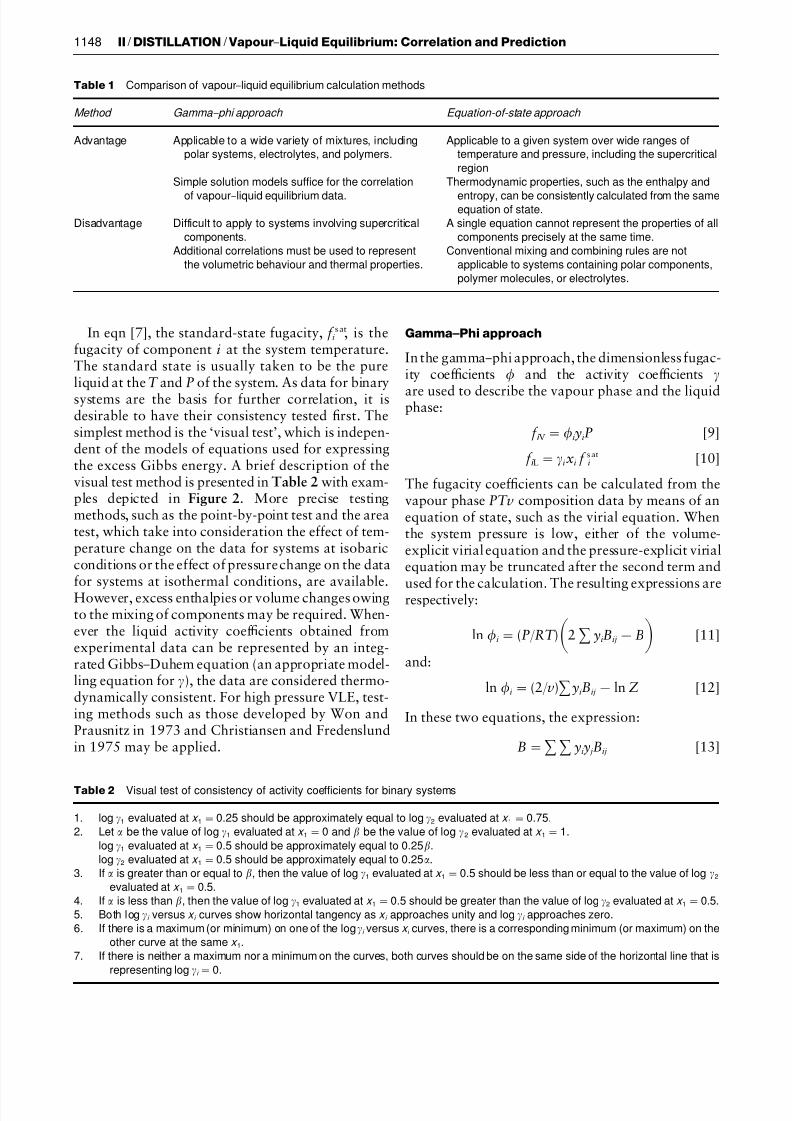
Table 2 Visual test of consistency of activity coefficients for binary systems

1. log 1 evaluated at x 1"0.25 should be approximately equal to log 2 evaluated at x 1"0.75.

2. Let be the value of log 1 evaluated at x 1"0 and be the value of log 2 evaluated at x 1"1.

log 1 evaluated at x 1"0.5 should be approximately equal to 0.25.

log 2 evaluated at x 1"0.5 should be approximately equal to 0.25.

3. If is greater than or equal to , then the value of log 1 evaluated at x 1"0.5 should be less than or equal to the value of log 2evaluated at x 1"0.5.

4. If is less than , then the value of log 1 evaluated at x 1"0.5 should be greater than the value of log 2 evaluated at x 1"0.5.

5. Both log i versus x i curves show horizontal tangency as x i approaches unity and log i approaches zero.

6. If there is a maximum (or minimum) on one of the log i versus x i curves, there is a corresponding minimum (or maximum) on the

other curve at the same x 1.

7. If there is neither a maximum nor a minimum on the curves, both curves should be on the same side of the horizontal line that is

representing log i "0.

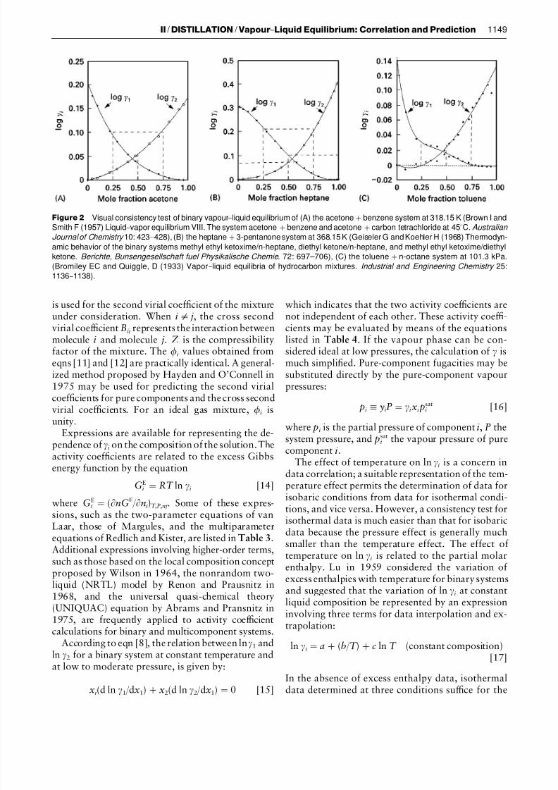
In eqn [7], the standard-state fugacity, f s ati , is thefugacity of component i at the system temperature.The standard state is usually taken to be the pureliquid at the T and P of the system. As data for binarysystems are the basis for further correlation, it isdesirable to have their consistency tested Rrst. Thesimplest method is the ‘visual test’, which is indepen-dent of the models of equations used for expressingthe excess Gibbs energy. A brief description of thevisual test method is presented in Table 2 with exam-ples depicted in Figure 2. More precise testingmethods, such as the point-by-point test and the areatest, which take into consideration the effect of tem-perature change on the data for systems at isobaricconditions or the effect of pressure change on the datafor systems at isothermal conditions, are available.However, excess enthalpies or volume changes owingto the mixing of components may be required. When-ever the liquid activity coef Rcients obtained fromexperimental data can be represented by an integ-rated Gibbs}Duhem equation (an appropriate model-ling equation for ), the data are considered thermo-dynamically consistent. For high pressure VLE, test-ing methods such as those developed by Won andPrausnitz in 1973 and Christiansen and Fredenslundin 1975 may be applied.

Gamma+Phi approach

In the gamma}phi approach, the dimensionless fugac-ity coef Rcients and the activity coef Rcients

are used to describe the vapour phase and the liquidphase:

f Ki V" KiyiP [9]

f Ki L"ixi f s ati [10]

The fugacity coef Rcients can be calculated from thevapour phase PTv composition data by means of anequation of state, such as the virial equation. Whenthe system pressure is low, either of the volume-explicit virial equation and the pressure-explicit virialequation may be truncated after the second term and

used for the calculation. The resulting expressions arerespectively:

ln Ki"(P/ RT )2 yiBij!B [11]

and:

ln Ki"(2/ v)yiBij!ln Z [12]

In these two equations, the expression:

B" yiy jBij [13]




Figure 2 Visual consistency test of binary vapour}liquid equilibrium of (A) the acetone#benzene system at 318.15 K (Brown I and

Smith F (1957) Liquid}vapor equilibrium VIII. The system acetone#benzene and acetone#carbon tetrachloride at 453C. Australian

Journal of Chemistry 10: 423I428), (B) the heptane#3-pentanone system at 368.15 K (Geiseler G and Koehler H (1968) Thermodyn-

amic behavior of the binary systems methyl ethyl ketoxime/n-heptane, diethyl ketone/n-heptane, and methyl ethyl ketoxime/diethyl

ketone. Berichte, Bunsengesellschaft fuel Physikalische Chemie . 72: 697I706), (C) the toluene#n-octane system at 101.3 kPa.

(Bromiley EC and Quiggle, D (1933) Vapor}liquid equilibria of hydrocarbon mixtures. Industrial and Engineering Chemistry 25:

1136}

1138).

is used for the second virial coef Rcient of the mixtureunder consideration. When iO j, the cross secondvirial coef Rcient Bij represents the interaction betweenmolecule i and molecule j. Z is the compressibilityfactor of the mixture. The i values obtained fromeqns [11] and [12] are practically identical. A general-ized method proposed by Hayden and O’Connell in1975 may be used for predicting the second virialcoef Rcients for pure components and the cross secondvirial coef Rcients. For an ideal gas mixture, K

i is

unity.Expressions are available for representing the de-

pendence of i on the composition of the solution. Theactivity coef Rcients are related to the excess Gibbsenergy function by the equation

GEi"RT ln i [14]

where GEi"(nGE/ ni)T ,P,nj. Some of these expres-

sions, such as the two-parameter equations of vanLaar, those of Margules, and the multiparameterequations of Redlich and Kister, are listed in Table 3.

Additional expressions involving higher-order terms,such as those based on the local composition conceptproposed by Wilson in 1964, the nonrandom two-liquid (NRTL) model by Renon and Prausnitz in1968, and the universal quasi-chemical theory(UNIQUAC) equation by Abrams and Pransnitz in1975, are frequently applied to activity coef Rcientcalculations for binary and multicomponent systems.

According to eqn [8], the relation between ln 1 andln 2 for a binary system at constant temperature andat low to moderate pressure, is given by:

xi(d ln 1/ dx1)#x2(d ln 2/ dx1)"0 [15]

which indicates that the two activity coef Rcients arenot independent of each other. These activity coef R-cients may be evaluated by means of the equationslisted in Table 4. If the vapour phase can be con-sidered ideal at low pressures, the calculation of ismuch simpliRed. Pure-component fugacities may besubstituted directly by the pure-component vapourpressures:

pi,yiP"ixi psati [16]

where pi is the partial pressure of component i, P thesystem pressure, and psat

i the vapour pressure of purecomponent i.

The effect of temperature on ln i is a concern indata correlation; a suitable representation of the tem-perature effect permits the determination of data forisobaric conditions from data for isothermal condi-tions, and vice versa. However, a consistency test forisothermal data is much easier than that for isobaricdata because the pressure effect is generally muchsmaller than the temperature effect. The effect of

temperature on ln i is related to the partial molarenthalpy. Lu in 1959 considered the variation of excess enthalpies with temperature for binary systemsand suggested that the variation of ln i at constantliquid composition be represented by an expressioninvolving three terms for data interpolation and ex-trapolation:

ln i"a#(b/ T )#c ln T (constant composition)[17]

In the absence of excess enthalpy data, isothermal

data determined at three conditions suf Rce for the




Table 3 Selected acitivity coefficient models

Name G E/ (RT ) ln i

Margules G E/ (RT )"x 1x 2(Ax 1#Bx 2) ln 1"x 22 [B #2(A!B )x 1]

ln 2"x 21 [A#2(B !A)x 2]

van Laar G E/ (RT )"ABx 1x 2/ (Ax 1#Bx 2) ln 1"A[1#Ax 1/ (Bx 2)]2

ln 2"B [1#Bx 2/ (Ax 1)]2

Redlich}Kister G E/ (RT )"x 1x 2 [A#B (x 1!x 2)#C (x 1!x 2)2

#D (x 1!x 2)3#2]

ln 1"a 1x 22#b 1x 32#c 1x 32#d 1x 42#2

ln 2"a 2x 21#b 2x 31#c 2x 31#d 2x 41#2

where: a 1"A#3B #5C #7D #2

b 1"!4(B #4C #9D )#2

c 1"12(C #5D )#2

d 1"!32D #2

a 2"A!3B #5C !7D #2

b 2"4(B !4C #9D )#2

c 2"12(C !5D )#2

d 2"32D #2

Wilson G E/ (RT )"! i x i ln ( j x j ij ) ln i "1!ln( j x j ij )!k [x k ki / ( j x j kj )]

NRTL G E

RT

"x 1x 2

21G 21

x 1#x 2G 21#

12G 12

x 2#x 1G 12

where: 12"g 12

RT , 21"

g 21

RT

ln 1"x 22

21

G 21

x 1#x 2G 212

#

12G 12

(x 2#x 1G 12)2

ln G 12"!a 1212, ln G 21"!a 1221 ln 2"x 2112

G 12

x 2#x 1G 122

#21G 21

(x 1#x 2G 21)2UNIQUAC G E"G E (combinatorial)#G E (residual) ln i "ln

i

x i #5q i ln

i

i

# j l i !r i

r j l j

G E (combinatorial)

RT "x 1 ln

1

x 1#x 2 ln

2

x 2

#5q 1x 1 ln1

1

#q 2x 2 ln2

2

!q i ln (i # j ji )# j q i ji

i # j ji !

ij j #i ij

G E (residual)

RT "!q 1x 1 ln (1#221)!q 2x 2 ln (2#112)

where: i "1, j "2 or i "2, j "1

1"x 1r 1

x 1r 1#x 2r 2, 1"

x 1q 1

x 1q 1#x 2q 2l i "

z

2(r i !q i )!(r i !1)

ln 21"!u 21

RT , ln 12"!

u 12

RT l j "

z

2(r j !q j )!(r j !1)

determination of isobaric data within a reasonable

range of temperatures. Similarly, if isobaric vapour}

liquid equilibrium data are available at three condi-tions, isothermal data can be obtained by the sameapproach and then tested for consistency. The num-ber of sets of vapour}liquid equilibrium data requiredcan be reduced when excess enthalpies are available,but generally one set of experimental values shouldbe used in the correlation. In the absence of therequired data for the determination of parameters ineqn [17], RT ln i at a given composition may beassumed to be constant as an approximation. Thecorrelated results can also be used for the prediction

purposes.

Equation-of-State Approach

Fugacities of both phases are represented in this ap-proach by the same equation of state, which providesa relationship between the intensive thermodynamicvariables T , P, v and composition. Such an equationmay be explicit in P or v. The pressure-explicit equa-tions in the form of:

P"P(T , v, x1, x2,2 , xn

1) [18]

are more useful for solving phase-equilibrium prob-lems. In terms of the fugacity coef Rcients, KiV ("f Ki V/ yiP) and KiL ("f Ki L/ xiP), formulation of

vapour}

liquid equilibria is based on the equilibrium




Table 4 Barker’s method for the determination of activity coefficients from experimental

data

At equilibrium:

f K li "f K vi

Kvi ,f K vi

y i P (by definition)

y i P Kvi "x i i f

li

Kli "f li

P , Ksati "

f sati

p sati

Therefore:

y i P Kvi "x i i li P

ln (y i P Kvi )"ln (x i i )#ln li #ln P

"ln (x i i )#ln sati #

v li

RT (P ! p sati )#ln p sati

Hence:

ln i "lny i P

x i p sati

#ln Kvi !ln sati !

v li (P ! p sati )

RT

For a binary system:

B "y 21B 11#2y 1y 2B 12#y 22B 22

Let:12"2B 12!B 11!B 22

Then:

B "y 1B 11#y 2B 22#y 1y 212

At low pressure:

Z "Pv I

RT "1#

BP

RT

ln Kv1"B 11#y 2212

RT P

For pure component i :

ln i "

P

0

(Z i !1)dP

P , Z i "1#

B ii P

RT ln sat

i " p sati

0

(Z i !1)dP

P "

B ii

RT p sati

ln 1"lny 1P

x 1 p sat1

#B 11#y 2212

RT P !B 11

RT p sat1 !

v l1(P ! p sat1 )

RT

"lny 1P

x 1 p sat1

#(B 11!v l1)(P ! p sat1 )

RT #

y 2212P

RT

Similarly:

ln 2"lny 2P

x 2 p sat2

#(B 22!v l2)(P ! p sat2 )

RT #

y 2112P

RT

Barker JA (1953) Determinationof activity coefficients from total-pressuremeasurements.

Australian Journal of Chemistry (1953) 6: 207}210.

equations:

yi KiV"xi KiL (i"1, 2,2 , N ) [19]

with both the KiV and KiL calculated from the equa-

tions:

RT ln Ki"

V

[(P/ ni)T ,V ,nj!RT / V ] dV !RT ln Z

[20]

The advantage of this approach is that it is applic-

able to calculations of VLE at high pressures and it




can also be used to obtain other conRgurational prop-erties such as enthalpy, entropy and volume changesof mixing, which are useful in the design of distilla-tion columns.

The Rrst equation of state with a theoretical foun-dation was proposed by van der Waals in 1873,several decades after the ideal gas equation of state

had been formulated. This equation not only yieldsqualitatively correct representation of the phase be-haviour of a real Suid, but also provides the basis of the principle of corresponding states. Hundreds of equations of state have been developed since the pub-lication of the van der Waals equation. They may betheoretical, semi-theoretical or empirical. However,most of the modiRcations are generally limited toa speciRc purpose.

In order to apply an equation of state to va-pour}liquid equilibrium calculations for pure compo-nents, a suitable equation should satisfy the threeconditions at a given saturation temperature:

vV,calc."vV, vL,calc."vL, f V,calc."f L,calc. [21]

Mixing and combining rules for the equation para-meters are required for extending its application tomixtures. However, most of the practical equationsavailable at present have their inherent advantagesand disadvantages and may not satisfy both of thevolumetric conditions.

The equations of state expressed in terms of poly-nomials in volume are of practical importance. ForVLE calculations, especially when the properties un-der consideration are limited to T , P and composi-tions, the simplest and frequently used form is thatwhich is cubic in v. In spite of their shortcomings,these cubic equations are the most frequently used inpractice at present. Currently, the most popular two-parameter cubic equations of state include theSoave}Redlich}Kwong equation (1972):

P"RT / (v!b)!a/ [v(v#b)] [22]

and the Peng}

Robinson equation (1976):

P"RT / (v!b)!a/ [v(v#b)#b(v!b)] [23]

Both equations can be obtained from a general formof a four-constant cubic equation of the van derWaals type:

P"RT / (v!b)!a/ [(v#c1b)(v#c2b)] [24]

Additional multiparameter cubic equations, whichare of the form represented by eqn [24] but developed

for improving the representations of pure-component

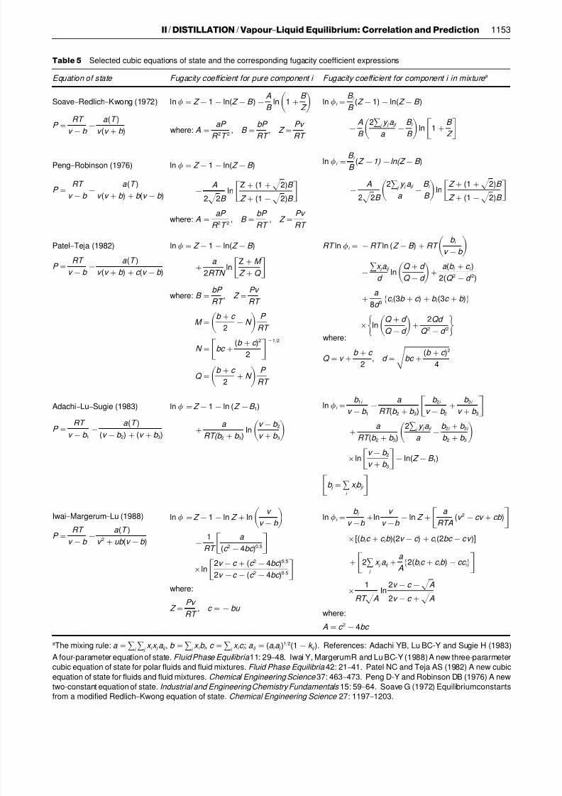
vapour pressures, saturated liquid volumes, the criti-cal compressibility factors, and phase behaviour of polar}nonpolar mixtures, appear continuously in theliterature. The maximum number of parameters ina cubic equation is Rve. A list of some selected cubicequations of state is presented in Table 5. In someof the cubic equations, different repulsion terms (the

Rrst term on the right-hand side of the equationslisted in the table) have been adopted. The forms of these equations are frequently inSuenced by the desireto improve the theoretical basis of the equation, andthat of Rtting the volumetric properties. It should alsobe mentioned that one of the inherent limitations of a two-parameter equation is that the critical com-pressibility factor is a constant for all components.The ability of a cubic equation in VLE representationis controlled by the selection of an adequate temper-ature function for the parameter ‘a’ for vapour pres-sures of pure components, and a set of suitable mix-ing and combining rules for all the parameters of theequation for mixtures.

Temperature function for ‘a ’ The importance of using a proper temperature function to represent theparameter ‘a’ cannot be overemphasized. In the1960s, Wilson began the consideration of the temper-ature effect on the parameter ‘a’ of theRedlich}Kwong equation. The expression which hasgained wider acceptance was developed by Soave forthe same equation in 1972. The parameter ‘a’ was

expressed by:

a"ac [25]

with expressed by a function involving the reducedtemperature T r ("T / T c) in the form:

"[1#m(1!T 1/ 2r )]2 [26]

where the subscript c refers to the critical-point con-dition, and m represents a quadratic function of theacentric factor of Pitzer. This form and its variations

have been adopted subsequently in many cubic equa-tions. A selected set of temperature functions for theparameter ‘a’ is listed in Table 6.

Mixing and combining rules To extend the applica-tion of his equation of state to representing the behav-iour of mixtures, van der Waals proposed that theconstants ‘a’ and ‘b’ be expressed by:

a"xix jaij [27]

a"xix jbij [28]




Table 5 Selected cubic equations of state and the corresponding fugacity coefficient expressions

Equation of state Fugacity coefficient for pure component i Fugacity coefficient for component i in mixture a

Soave}Redlich}Kwong (1972) ln "Z !1!ln(Z !B )!A

B ln 1#

B

Z ln i "B i

B (Z !1)!ln(Z !B )

!A

B 2

j y j a ji

a !

B i

B ln 1#B

Z P "RT

v !b !

a (T )

v (v #b ) where: A"aP

R

2

T

2, B "

bP

RT

, Z "Pv

RT

Peng}Robinson (1976) ln "Z !1!ln(Z !B )

!A

2 2B ln

Z#(1# 2)B

Z #(1! 2)B

ln i "B i

B (Z !1) !ln(Z !B )

!A

2 2B 2

j y j a ji

a !

B i

B ln Z #(1# 2)B

Z #(1! 2)B P "RT

v !b !

a (T )

v (v #b )#b (v !b )

where: A"aP

R 2T 2, B "

bP

RT , Z "

Pv

RT

RT ln i "!RT ln (Z !B )#RT b i

v !b !

x j a ij

d

ln

Q #d

Q !d

#

a (b i #c i )

2(Q 2

!d 2

)

#a

8d 3 c i (3b #c )#b i (3c #b )

ln Q #d

Q !d #2Qd

Q 2!d 2

Patel}Teja (1982) ln "Z !1!ln(Z !B )

#a

2RTN ln

Z#M

Z #Q P "RT

v !b !

a (T )

v (v #b )#c (v !b )

where: B "bP

RT , Z "

Pv

RT

M "b #c

2!N

P

RT

N "bc #(b #c )2

2

1/ 2 where:

Q "b #c

2#N

P

RT

Q "v #b #c

2, d " bc #

(b #c )2

4

Adachi}Lu}Sugie (1983) ln "Z !1!ln (Z !B 1)

#a

RT(b 2#b 3)ln

v !b 2

v #b 3

ln i "b 1i

v !b 1!

a

RT (b 2#b 3) b 2i

v !b 2#

b 3i

v #b 3#

a

RT (b 2#b 3) 2

j y j a ji

a !

b 2i #b 3i

b 2#b 3ln

v !b 2

v #b 3!ln(Z !B 1)

b j "i

x i b ji

P "RT

v !b 1!

a (T )

(v !b 2)#(v #b 3)

Iwai}Margerum}Lu (1988) ln "Z !1!ln Z #ln v

v !b !

1

RT a

(c 2!4bc )0.5ln

2v !c #(c 2!4bc )0.5

2v !c !(c 2!4bc )0.5

ln i "b i

v !b #ln

v

v !b !ln Z #

a

RTA(v 2!cv #cb )

[(b i c #c i b )(2v !c )#c i(2bc !cv )]

#

2

j

x j a ij #a A2(b i c #c i b )!cc i

1

RT Aln

2v !c ! A

2v !c # A

P "RT

v !b !

a (T )

v 2#ub (v !b )

where:

where:Z "

Pv

RT , c "!bu

A"c 2!4bc

aThe mixing rule: a "i

j x i x j a ij , b "

i x i b i , c "

i x i c i ; a ij "(a i a j )

1/ 2(1!k ij ). References: Adachi YB, Lu BC-Y and Sugie H (1983)

A four-parameter equation of state. Fluid Phase Equilibria 11: 29}48. Iwai Y, MargerumR and Lu BC-Y (1988) A new three-pararmeter

cubic equation of state for polar fluids and fluid mixtures. Fluid Phase Equilibria 42: 21}41. Patel NC and Teja AS (1982) A new cubic

equation of state for fluids and fluid mixtures. Chemical Engineering Science 37: 463}473. Peng D-Y and Robinson DB (1976) A new

two-constant equation of state. Industrial and Engineering Chemistry Fundamentals 15: 59}64. Soave G (1972) Equilibriumconstants

from a modified Redlich}

Kwong equation of state. Chemical Engineering Science 27: 1197}

1203.




Table 6 Some different forms of the function

Form Reference

"1#m (1!T r) 1"[1#m (1! T r)]2 2

"[1#m 1(1! T r)#m 2(1/ T r!1)]2 3

"[1#m 1(1! T r)#m 2(1!T r)(0.7!T r)]2 4

"1#m 1(1!T r)#m 2(1/ T r!1) 5"10[m (1

T r)] 6

"1#[m 1#m 2(1# T r)(0.7!T r)](1! T r)2 7

"10f (T r), f (T r)"m 3(m 0#m 1T r#m 2T 2r )(1!T r) 8

"exp[m 1(1!T r)#m 2(1! T r)2] 9

"T (m 21)m 3

r exp [m 1(1!T m 2Hm 3r )] 10

References: 1. Wilson GM (1964) VaporIliquid equilibriums, cor-

relation by means of a modified Redlich}Kwong equation of state.

Advances in Cryogenic Engineering . 9: 168}176. 2. Soave G

(1972) Equilibrium constants from a modified Redlich}Kwong

equation of state. Chemical Engineering Science 27:

1197}1203. 3. Harmens A and Knapp H (1980) Three-parameter

cubic equation of state for normal substances. Industrial and

Engineering Chemistry Fundundamentals 19: 291}

294. 4.Mathias PM (1983) A versatile phase equilibrium equation of

state. Industrial and Engineering Chemistry. Process Design and

Development 22: 385}391. 5. Soave G (1984) Improvement of

the van der Waals equation of state. Chemical Engineering

Science 39: 357}369. 6. Adachi Y and Lu BC-Y (1984) Simplest

equation of state for vapor}liquid equilibrium calculations: a modi-

fication of the van der Waals equation. American Institute of

Chemical Engineers Journal 30: 991}993. 7. Stryjek R and Vera JH

(1986) PRSV: An improved Peng}Robinson equation of state for

pure compounds and mixtures. Canadian Journal of Chemical

Engineering 64: 323}333. 8. Yu JM and Lu BC-Y (1987) A three-

parameter cubic equation of state for asymmetric mixture density

calculations. Fluid Phase Equilibria 34: 1}19. 9. Melhem GA,

Saini R and Goodwin BM (1989) A modified Peng}Robinson

equation of state. Fluid PhaseEquilibria 47: 189}237. 10. Twu CH,

Bluck D, Cunnigham JR and Coon JE (1991) A cubic equation of

state with a new alpha function and a new mixing rule. Fluid

Phase Equilibria 69: 33}50.

Table 7 Some mixing and combining rules for cubic equations

of state

van der Waals/ Berthelot

a ij "(a i a j )1/ 2

a "i

j

y i y j a ij , b "i

y i b i

Modified van der Waals/ Berthelot

a " y i y j a ij b " y i y j b ij

a ij "(a i a j )1/ 2(1!k ij )

b ij "12(b i #b j )(1!c ij )

Wong}Sandler

b !a

RT "

i

j b ij !

a ij

RT b ij "

b i #b j

2(1!k ij )

a ij "a i #a j

2(1!k ij )

a

b "

x i a i

b i !

G E

CRT

where: G E is a selected excess Gibbs energy model

C is characteristic of the equation of state

The simplest combining rules for ‘aij’ and ‘bij’ areobtained by using the geometric mean for aij and thearithmetic mean for b ij, i.e:

aij"(aia j)1/ 2 [29]

bij"(bi#b j)/2 [30]

A binary interaction parameter kij is frequently intro-duced in eqn [29] to correct the discrepancy gener-ated by the geometric mean:

aij"(aia j)1/ 2(1!kij) [31]

Occasionally, a binary interaction parameter l ij isintroduced in eqn [30] to yield improved b ij values:

bij"(bi#b j)(1!l ij)/ 2 [32]

More recently, new mixing rules, such as the one

proposed by Wong and Sandler in 1992, with im-

proved theoretical considerations have appeared inthe literature. A list of some mixing and combiningrules is presented in Table 7.

In general, vapour}liquid equilibrium of a greatvariety of mixtures, including polar}nonpolar mix-tures, can be well represented. For a given mixture,the equation-of-state mixing rules with one set of

parameters can frequently represent the data overwide ranges of temperature and pressure.

Examples of binary data representation by meansof the two approaches are depicted in Figure 3.

Prediction of Vapour}Liquid Equilibria

Although vapour}liquid equilibria have been investi-gated for more than 10 000 systems, values resultingfrom various combinations are still unknown. Itwould be impractical to determine experimentally allthe systems needed individually.

In principle, experimental values of some thermo-dynamic properties can be used to estimate otherproperties. For examples, binary vapour}liquid equi-librium can be estimated from the liquid activitycoef Rcients calculated from mutual solubility data forthe same mixture, and the inRnite-dilution activitycoef Rcients measured from gas}liquid chromatogra-phy can be used to predict the vapour}liquid equilib-ria over the complete concentration range. Some pre-diction methods are brieSy described below with em-phasis placed on binary mixtures. Extending the




Figure 3 (A) Correlating the phase behaviourof the (ethanol#benzene) systemat 323.15 K by meansof the gamma}phi approach.

The lines represent the values calculated by using the Margules equations and the points represent the experimental values reported

by ND. Litvinov (1952) Isothermal equilibrium of vapor and liquid in systems of three fully miscible liquids. Zhurnal Fizicheskoi Khimii 26: 1405}1412. (B) Predicting the phase behaviour of the (0.2654 mole fraction ethane#0.7346 mole fraction n -heptane) mixture by

means of the equation-of-state approach. The smooth curve represents the values calculated by using the Peng }Robinson equation,

and the points represent the experimental values reported by WB Kay (1938) Liquid}vapor phase equilibrium relations in the

ethane-n-heptane system. Industrial and Engineering Chemistry 30: 459}464.

application to multicomponent mixtures is feasibleonce good correlation of the vapour}liquid equilibriaof its constituent binary systems becomes available.

Prediction from Pure Component Properties

Application of the regular solution theory For mix-tures containing nonpolar components that are notmuch different in size and shape, the regular solutiontheory of Hildebrand leads to a semi-quantitativeprediction of k values of all components in a mixture.In terms of the solubility parameter, the activity co-ef Rcients of the components in a regular solution canbe calculated from the equation:

RT ln k"vk(k!)2 [33]

where the volume average solubility parameter is

given by:

"ii [34]

and the volume fraction i is deRned by:

i"xivi/ x jv j [35]

The solubility parameter for substance k, k, is de-Rned by:

k"(U V

k / vV

k )1/ 2

"[(H V

k!RT )/ vk]1/ 2

[36]

where U Vk and H Vk are, respectively, the molar en-ergy and enthalpy of vaporization of pure liquid k attemperature T . The assumption involved here is thatT is well below the critical temperature in order tomake the approximation valid. The calculated liquidactivity coef Rcients can then be used to obtainthe desired vapour}liquid equilibrium values. For abinary mixture:

RT ln 1"v122(1!2)2 [37]

RT ln 2"v221(1!2)2 [38]

Should a binary interaction parameter be requiredto improve the data representation, an extension of the approach to the prediction of multicomponentvapour}liquid equilibrium may not be practical;attempts made to correlate the binary parameters

have not been successful.

Liquid activity coef Vcients at inVnite dilution

Values of are particularly useful for obtaining theparameters of any of the two-constant equations forthe excess Gibbs energy; the values for a binarysystem are the parameter values. For example,1"A and 2"B for the van Laar and Margulesequations presented in Table 3. If a three-parameterequation is used, the third parameter must be deter-mined by an independent approach.

The modiRed separation of cohesive energy density

(MOSCED) method proposed by Thomas and Eckert




in 1984 may be used to predict values from purecomponent parameters. This method is based ona modiRed regular solution theory and the assump-tion that the forces contributing to the cohesiveenergy are additive. It has been reported that theaverage error of 3357 values predicted by thismethod was 9.1%.

In general, calculated equilibrium vapour composi-tions are relatively insensitive to moderate errors inthe used in the calculation.

Prediction of Binary Values Using Azeotropic or

Mutual Solubility Data

Prediction from azeotropic data Many binary sys-tems exhibit azeotropic behaviour. At an azeotropiccondition, the compositions of the liquid and vapourphases are identical. At low pressures, the liquid ac-tivity coef Rcients can be simply calculated by:

1"P/ psat1 and 2"P/ psat

2 [39]

The parameters of any two-parameter expression of the excess Gibbs energy can then be obtained andused for extrapolating vapour}liquid equilibriumover the complete concentration range.

Prediction of values from mutual solubility dataThe thermodynamic consideration applicable to a bi-nary system at vapour}liquid equilibrium is also ap-plicable to a partially miscible binary liquid mixture

at equilibrium. Hence, the activity coef Rcients of thetwo liquids at the temperature at which the solubili-ties were experimentally determined can be expressedby:

1x1"1x1 and 2x2"2x2 [40]

where the two superscripts refer to the two liquidphases. Applying these relationships to any two-para-meter expression of the excess Gibbs energy leads tothe determination of the parameter values, whichpermit vapour}liquid equilibrium estimation of themixture.

Prediction of from Group Contribution Methods

In group contribution methods, the calculation of thermodynamic properties of pure Suids is based onthe assumption that each molecule is an aggregate of functional groups. Langmuir in 1925 extended theconcept to mixtures. Redlich, Derr, Pierotti andPapadopoulos developed a group interaction modelfor heats of solution in 1959. Adopting the conceptspresented by these authors, Wilson and Deal sugges-

ted in 1962 a solution of the groups approach by

which liquid activity coef Rcients can be estimated onthe basis of group contributions. In this approach, thelogarithm of the activity coef Rcient of a component isassumed to be the sum of two contributions: theconRgurational contribution, which accounts for thedifferences in molecular size, and the group interac-tion contribution, which accounts for the inter-

molecular forces originating from the different func-tional groups.

The group contribution approach to calculating isattractive because through this approach it is possibleto estimate vapour}liquid equilibria of nonideal mix-tures without experimentation. Although a largenumber of mixtures can result from pure compounds,the functional groups, such as CH2, OH, CO, COOand COOH, that constitute these compounds arelimited. If the activity coef Rcients of the mixturecomponents could be obtained from a knowledge of the interactions of these groups, and with the assump-tion that the contribution to by one group withina molecule is independent of that made by any othergroup in that molecule, a relatively small number of parameters would suf Rce for the prediction of theactivity coef Rcients for mixtures containing the samegroups. This assumption implies that the contributionof the group interaction is independent of the natureof the molecule.

Two of these approaches are mentioned here.

Analytical solutions of groups (ASOG) methodFollowing the concept of the solutions of groups of Wilson and Deal, the analytical solutions of groups(ASOG) method was Rrst presented by Derr and Dealin 1969. Basically, the practical application of thesolutions of groups concept involves the reduction of liquid activity coef Rcients obtained from experi-mental data for vapourd liquid equilibria into a num-ber of binary group interaction parameters. Theworking equations of the ASOG method are present-ed in Table 8.

Kojima and Tochigi in 1979 calculated the groupinteraction parameters for 31 groups and used the

method to predict the vapour}

liquid equilibria for936 binary systems, 103 ternary systems, Rve quater-nary systems, and two quinary systems at low pres-sures. They reported that the average absolute devi-ation of the predicted vapour compositions was 1.2%.

Universal functional group activity coef Vcient(UNIFAC) method The universal functional groupactivity coef Rcient (UNIFAC) method proposed byFredenslund, Gmehling and Rasmussen and theASOG method are based on the same principle of group contributions. The main difference between

these two methods is in the equations used for




Table 8 The analytical solution of groups (ASOG) method

1. ln i "ln Si#ln Gi 2. ln Si "1!r i !ln r i

where:r i "

v i

x j v j x j "mole fraction of molecule j

v j "number of atoms other than hydrogen in mol-

ecule j

3. ln Gi "k

v ki (ln k !ln (i )k )

where: v ki "number of atoms other than hydrogen in

group k in molecule i

ln k "1!C k !ln D k ln (i )

k "1!C (i )k !ln D (i )k

C k " j

X j A jk

D j , C (i )k "

X (i ) j A jk

D j

D k "X j Akj , D (i )k "X (i ) j Akj

X L"1

S x i v Li , X (i )L"

v Li

k v ki

AkL"expm kL#n kL

T S "

i

x i k

v ki

Table 9 The UNIFAC method

1. ln i "ln ci #ln Ri

2. ln ci "1!J i #ln J i !5q i 1!J i

Li

#lnJ i

Li where:

J i "r i

j x j r j

, Li "q i

x j q j

r i "k

v (i )k R k , q i "k

v (i )k Q k

R k "volume parameter for group k

Q k "surface area parameter for group k

v (i )k "number of subgroups of type k in molecule

of species i

3. ln Ri "q i 1!k

k ik

S k !ki ln

ik

S k where:

ki "v (i )k Q k

q i ik "

m mi mk

k "

i x i q i ki

j x j q j

S k "m m mk

mk "exp!mk

T mk "group interaction parameter

representing the excess Gibbs energy. The Wilsonequation is used in the ASOG method, whereas thetwo-parameter universal quasi-chemical (UNIQUAC)equation of Abrams and Prausnitz is used in theUNIFAC method. The working equations of theUNIFAC method are presented in Table 9. There are50 main groups together with their subgroups for thedetermination of the parameters involved in the cal-culation. For calculations for multicomponent sys-tems, the adjustable binary parameters are evaluatedfrom binary vapour}liquid equilibrium data.

Prediction using Equations of State

The equations of state successfully used for correlationof binary vapour}liquid equilibria can be used for thepurposes of predicting multicomponent vapour}liquid

equilibria, provided that the binary interaction para-meters of all the constituent binary systems are avail-able. All the parameters should be obtained by regres-sion of the binary data using the same mixing andcombining rules. Interpolated and estimated values of these parameters are available for some systems, buttheir values are subject to frequent revision.

Additional Comments on Applications

There is no simple equation of state that can represent

satisfactorily the three conditions of eqn [21] over

a wide range of temperature. Experience indicatesthat equations that could meet the equal fugacitycondition as well as vV or vL would be suitable for theintended vapour}liquid equilibrium calculations.Should a situation arise such that the saturated liquidmolar volume is required in the estimation, cubicequations containing more parameters may be se-

lected for the representation. Adachi and Lu in 1990suggested that it is possible to assign different two-parameter or three-parameter cubic equations to dif-ferent components of the binary mixture underconsideration, and then use a four-parameter cubicequation to combine the equations in thevapour}liquid equilibrium calculations for mixtures.

Special case should be applied when equations of state are used to represent the experimental datameasured at or near theoretical points of the Suids.

The selection of mixing and combining rules playsa crucial role in the application of equations of stateto the correlation and prediction of vapourd liquidequilibria. The importance of selecting an appropri-ate expression for the excess Gibbs energy cannot beoveremphasized.

The prediction of binary vapour}liquid equilibriafrom pure-component properties by means of theMOSCED method is attractive. However, poor re-sults are obtained for systems where steric consider-ations are signiRcant. The general applicability of thismodel is limited due to the dif Rculties involved in




Figure 4 Algorithms for correlating and predicting vapour}liquid equilibrium values.

the determination of pure component parameters. Fur-

thermore, the approach cannot be used for aqueousmixtures, nor for systems with very large values.In general, the accuracy of prediction depends on

the availability of some reliable binary data for eitherthe system of interest or another one that is closelyrelated to it.

All the group-contribution methods are approxim-ate. The fundamental assumption involved in thegroup solution approach is additivity, and the esti-mated values are necessarily approximate.

Finally, computer software packages for vapour}liquid equilibrium calculations are available commer-

cially from a number of process engineering software

development companies. Typical algorithms for data

correlation and prediction are depicted in Figure 4.

See also: II/Distillation: Modelling and Simulation;

Multicomponent Distillation; Theory of Distillation; Vapour-

Liquid Equilibrium: Theory. III/Physico-Chemical Meas-

urements: Gas Chromatography.

Further Reading

Abrams DS and Prausnitz JM (1975) Statistical thermo-dynamics of liquid mixtures. New equation for the ex-cess Gibbs energy of partly or completely miscible sys-tems. American Institute of Chemical Engineering Jour-

nal 21: 116}

128.




Adachi Y and Lu BC-Y (1990) Taking advantage of avail-able cubic equations of state. Canadian Journal of Chemical Engineering 68: 639}644.

Christiansen LJ and Fredenslund A (1975) Thermodynamicconsistency using orthogonal collocation or compositionof equilibrium vapor compositions at high pressures.American Institute of Chemical Engineers Journal 21:

49}

57.Derr EL and Deal CH Jr (1969) Analytical solutions of groups. Correlation of activity coef Rcients throughstructural group parameters. Proceedings of Interna-tional Symposium of Distillation 3: 40}51.

Denbigh K (1981) The Principles of Chemical Equilibrium,4th edn. Cambridge: Cambridge University Press.

Fredenslund A, Gmehling J and Rasmussen P (1977) Va- pour}Liquid Equilibria Using UNIFAC. Amsterdam:Elsevier.

Gmehling J, Onken U and Arlt W (1974}1990) Vapour}Liquid Equilibrium Data Collection; Dechema Chem-istry Data Series, vol. I, parts 1}8. Frankfurt: Dechema.

Hala E, Pick J, Fried V and Vilim O (1967) Vapour}

Liquid Equilibrium, 2nd edn. Oxford: Pergamon Press.Hayden JG and O’Connell JP (1975) Generalized method

for predicting second virial coef Rcients. Industrial and Engineering Chemistry. Process Design and Develop-ment 14: 209}216.

Knapp H, Doring R, Oellrich L, Plocker U and Prausnitz JM (1982) In: Behrens D and Eckerman R (eds) Chem-istry Data Series, Vol. VI: VLE for Mixtures of LowBoiling Substances. Frankfurt: Dechema.

Kojima K and Tochigi T (1979) Prediction of Vapour}Liquid Equilibria by the ASOG Method . New York:Elsevier.

Lewis, GN and Randall M (1923) Thermodynamics and the Free Energy of Chemical Substances. New York:McGraw-Hill.

Lu BC-Y (1959) Heats of mixing and vapor}liquid equilib-rium calculations. Canadian Journal of Chemical Engine-ering 37: 193}199.

Lu BC-Y (1962) Binary vapor}liquid equilibrium data:Thermodynamic consistency tests. Canadian Journal of Chemical Engineering 40: 16}24.

Malanowski S and Anderko A (1992) Modelling PhaseEquilibria, Thermodynamic Background and Practical Tools. New York: John Wiley.

Papadopoulos MN and Derr EL (1959) Group interaction.II. A test of the group model on binary solutions of hydrocarbons. Journal of American Chemical Society81: 2285}2289.

Prausnitz JM, Lichtenthaler RN and de Azevedo EG(1999) Molecular Thermodynamics of Fluid-PhaseEquilibria, 3rd edn. Englewood Cliffs, NJ: Prentice-

Hall.Raal JD and Muhlbauer AL (1998) Phase Equilibria,Measurement and Computation. Washington, DC:Taylor & Francis.

Redlich O, Derr EL and Pierotti GJ (1959) Group interac-tion. I. A model for interaction in solutions. Journal of American Chemical Society 81: 2283}2285.

Reid RC, Prausnitz JM and Poling BE (1987) The Proper-ties of Gases and Liquids, 4th edn. New York: McGraw-Hill.

Renon H and Prausnitz JM (1968) Local compositions inthermodynamic excess functions for liquid mixtures.American Institute of Chemical Engineers Journal 14:

135}

144.Starling KE (1977) Fluid Properties for Light PetroleumSystems. Houston, TX: Gulf Publishing Co.

Thomas ER and Eckert CA (1984) Prediction of limitingactivity of coef Rcients by a modiRed separation of cohe-sive energy density model and UNIFAC. Industrial and Engineering Chemistry. Process Design and Develop-ment 23: 194}209.

Walas SM (1985) Phase Equilibria in Chemical Engineer-ing . Boston: Butterworth.

Wilson GM (1964) Vapor}liquid equilibrium. XI. A newexpression for the excess Gibbs energy of mixing. Jour-nal of American Chemical Society 86: 127}130.

Wilson GM and Deal CH (1962) Activity coef Rcients andmolecular structure} activity coef Rcients in changing en-vironments} solutions of groups. Industrial and Engin-eering Chemistry Fundamentals 1: 20}23.

Won KW and Prausnitz JM (1973) High-pressure vapor}liquid equilibriums. Calculation of partial pressuresfrom total pressure data. Thermodynamic consistency.Industrial and Engineering Chemistry Fundamentals 12:459}463.

Wong DSH and Sandler SI (1972) A theoretically correctmixing rule for cubic equations of state. American Insti-tute of Chemical Engineers Journal 38: 671}680.

Vapour}Liquid Equilibrium: Theory

A. S. Teja and L. J. Holm, Georgia Institute of

Technology, Atlanta, GA, USA

Copyright^ 2000 Academic Press

Introduction

The concept of an equilibrium stage in distillation is

based on the assumption that the vapour leaving the

stage is in equilibrium with the liquid leaving thesame stage. The use of this concept in the design of distillation columns requires a description of how thecomponents of a multicomponent mixture distributebetween the two phases in equilibrium. This descriptionis provided by phase equilibrium thermodynamics.

The equilibrium relationship for any component

i in an equilibrium stage is deRned in terms of the

II / DISTILLATION / Vapour}Liquid Equilibrium: Theory 1159

vapor liquid

Documents