valuing public sector risk exposure in transportation public … · 2018-09-28 · rafael aldrete,...

Rafael Aldrete, Arturo Bujanda and Gabriel A. Valdez-Ceniceros

DOT Grant No. DTRT06-G-0044

Valuing Public Sector Risk Exposure in Transportation Public-Private Partnerships

Final Report

Performing OrganizationUniversity Transportation Center for Mobility™Texas Transportation InstituteThe Texas A&M University SystemCollege Station, TX

Sponsoring AgencyDepartment of TransportationResearch and Innovative Technology AdministrationWashington, DC

“Improving the Quality of Life by Enhancing Mobility”

University Transportation Center for Mobility

UTCM Project # 08-41-01October 2010

Technical Report Documentation Page 1. Report No. UTCM 08-41-01

2. Government Accession No.

3. Recipient's Catalog No.

4. Title and Subtitle VALUING PUBLIC SECTOR RISK EXPOSURE IN TRANSPORTATION PUBLIC-PRIVATE PARTNERSHIPS

5. Report Date October 2010 6. Performing Organization Code Texas Transportation Institute

7. Author(s) Rafael M. Aldrete, Arturo Bujanda, and Gabriel A. Valdez-Ceniceros

8. Performing Organization Report No. Report UTCM 08-41-01

9. Performing Organization Name and Address University Transportation Center for Mobility Texas Transportation Institute The Texas A&M University System 3135 TAMU College Station, Texas 77843-3135

10. Work Unit No. (TRAIS) 11. Contract or Grant No. DTRT06-G-0044

12. Sponsoring Agency Name and Address Department of Transportation Research and Innovative Technology Administration 400 7th Street, SW Washington, DC 20590

13. Type of Report and Period Covered Final Report: 9/1/2008-10/31/2010 14. Sponsoring Agency Code

15. Supplementary Notes Supported by a grant from the U.S. Department of Transportation, University Transportation Centers Program Project Title: Developing a Methodological Framework to Value Public Sector’s Risk Exposure in PPP Agreements 16. Abstract This report presents a methodological framework to evaluate public sector financial risk exposure when delivering transportation infrastructure through public-private partnership (PPP) agreements in the United States (U.S.). The framework is based on U.S. and international best practices to quantify public sector risk exposure in infrastructure. Transportation agencies worldwide and across the U.S. are increasingly using PPPs as a mechanism to deliver much needed transportation infrastructure. The key premises behind the increased use of PPPs as project delivery mechanisms are the interdependent concepts of value for money (VfM) and the optimum allocation of project risks to the partner most capable to manage them. Internationally, countries with relatively longer experience in PPPs have devised different methodological approaches to measure and manage risk exposure, and a handful of other countries have developed more sophisticated and well-documented methodologies to value risk in the context of VfM. However, transportation agencies in the U.S. have not developed structured processes to measure risk exposure and to integrate the cost of risk bearing into the process of evaluating PPP projects. More specifically, U.S. transportation agencies—including agencies in Texas—currently lack a well-documented approach to consistently evaluate and account for public sector financial risk exposure in a PPP, and a methodology to incorporate the cost of risk bearing in the analysis of PPP projects. 17. Key Words Public-private partnerships, PPP, comprehensive development agreement, transportation reinvestment zone, TRZ, public sector risk, contingent liabilities, guarantees, policy

18. Distribution Statement Public Distribution

19. Security Classif.(of this report) Unclassified

20. Security Classif.(of this page) Unclassified

21. No. of Pages 73

22. Price n/a

Form DOT F 1700.7 (8-72) Reproduction of completed page authorized

VALUING PUBLIC SECTOR RISK EXPOSURE IN TRANSPORTATION PUBLIC-PRIVATE PARTNERSHIPS

by

Rafael M. Aldrete, Ph.D. Research Scientist

Texas Transportation Institute

Arturo Bujanda Associate Research Specialist Texas Transportation Institute

and

Gabriel A. Valdez-Ceniceros Graduate Research Assistant


Final Report Project 08-41-01

October 2010

TEXAS TRANSPORTATION INSTITUTE The Texas A&M University System College Station, Texas 77843-3135

2

DISCLAIMER

The contents of this report reflect the views of the authors, who are responsible for the facts and the accuracy of the information presented herein. This document is disseminated under the sponsorship of the U.S. Department of Transportation, University Transportation Centers Program in the interest of information exchange. The U.S. Government assumes no liability for the contents or use thereof.

ACKNOWLEDGMENTS

Support for this research was provided in part by a grant from the U.S. Department of Transportation, University Transportation Centers Program to the University Transportation Center for Mobility (DTRT06-G-0044).

Additional in-kind support for this research was provided by Castalia Strategic Advisors, who contributed crucial research and insight into the review and analysis of international practices.

The authors also acknowledge the in-kind contribution of Dr. Cesar Queiroz and Dr. Samuel Mintz, who provided invaluable feedback into the overall report.

The authors thank the project monitor, Eduardo Calvo, Director of Transportation Planning at the El Paso District of the Texas Department of Transportation, for his invaluable guidance, support and feedback in conducting this research.

3

TABLE OF CONTENTS

Page List of Figures ................................................................................................................................ 5 List of Tables ................................................................................................................................. 5 List of Boxes................................................................................................................................... 6 Executive Summary ...................................................................................................................... 7

The Problem ................................................................................................................................ 7 Research Approach and Methodology ........................................................................................ 7 Research Findings ....................................................................................................................... 8 Research Conclusions ................................................................................................................. 8 Research Recommendations ....................................................................................................... 9

Chapter 1: Introduction ............................................................................................................. 11 Research Need .......................................................................................................................... 11 Research Objective ................................................................................................................... 12 Structure of the Report .............................................................................................................. 12

Chapter 2: Value for Money and Valuing Project Risk in Public-Private Partnerships ..... 13 Public-Private Partnerships in Infrastructure, Risk, and Value for Money .............................. 13

What is a PPP? ...................................................................................................................... 13 What is Risk, Managing Risks, and Value for Money ......................................................... 15

Government Support and Risk Exposure in PPP Projects ........................................................ 19 Guarantees, Contingent Liabilities, and Risk Exposure in PPP Projects .............................. 20 The Need for a Framework to Value Risk Exposure ............................................................ 21

Chapter 3: Public Risk in Infrastructure PPPs—International Practices and Lessons Learned ........................................................................................................................................ 23

Dealing with PPP Public Sector Risk Exposure in the United States ....................................... 23 Texas Sam Rayburn Tollway ................................................................................................ 24 Texas State Highway 130 Segments 5 & 6 ........................................................................... 25 Indiana Toll Road ................................................................................................................. 26 Chicago Skyway Toll Road .................................................................................................. 27

International Experience Dealing with PPP Public Sector Risk Exposure ............................... 27 Colombia ............................................................................................................................... 28 South Africa .......................................................................................................................... 29 Chile ...................................................................................................................................... 31 Victoria, Australia ................................................................................................................. 34

Lessons from the International Practice .................................................................................... 36 Common Functions and Features of Risk Exposure Management Frameworks .................. 36 Applicability of International Experience to Valuation of Risk Exposure in U.S. PPPs ...... 37

Chapter 4: Valuing Public Sector Risk in Transportation PPP Projects .............................. 39 Risk Measurement .................................................................................................................... 39 Methods for Valuing Guarantees and Contingent Liabilities ................................................... 40

Contingent Liability Valuation Methods .............................................................................. 40 Contingent Claims Analysis Approach to Guarantee Valuation .......................................... 41

Valuing Public Sector PPP Risk Exposure as a Contingent Liability ...................................... 45 Applicability and Limitations ............................................................................................... 46

4

Methodological Framework Overview ................................................................................. 46 Methodology Application ..................................................................................................... 48

Chapter 5: Valuation of Public Sector Risk Exposure in U.S. Transportation PPP Project Case Studies ................................................................................................................................. 51

César Chávez Toll Road Project Case Study ............................................................................ 51 Toll Revenue Forecast Volatility .......................................................................................... 53 César Chávez Toll Road—Contingent Claims Analysis ...................................................... 57

Transportation Reinvestment Zone Project Case Study ........................................................... 59 Value Capture as a PPP—The Texas TRZ Model and Revenue Risk Characteristics ......... 59 The City of El Paso TRZ No. 2 and 3 ................................................................................... 61 City of El Paso TRZ No. 2 and 3—Contingent Claims Analysis ......................................... 64

Chapter 6: Conclusions and Recommendations ...................................................................... 67 Conclusions ............................................................................................................................... 67 Recommendations ..................................................................................................................... 68

References .................................................................................................................................... 71

5

LIST OF FIGURES

Page Figure 1: Amount of Risk Shared for Different Types of PPP Contracts (4) ............................... 15 Figure 2: Risk Management Process............................................................................................. 16 Figure 3: Optimal Total Project Risk Allocation (6) .................................................................... 18 Figure 4: VfM Comparison Using the Public Sector Comparator (Adapted from [7]) ................ 19 Figure 5: Sam Rayburn Tollway Economic Benefit Comparison—NTTA vs. Cintra (18) ......... 25 Figure 6: Transferrable Risk Distribution and Mean—Australia Example (29) .......................... 35 Figure 7: Measuring Risk Using Probability Distribution Functions ........................................... 40 Figure 8: Stochastic Analysis Using Monte Carlo Simulation ..................................................... 45 Figure 9: Histogram of Guarantee Values—Example .................................................................. 47 Figure 10: Step-by-Step Methodology to Value Public Sector Risk Exposure in PPPs ............... 48 Figure 11: Potential Managed Lanes on the Border Highway (El Paso Loop 375) ..................... 52 Figure 12: César Chávez Toll Road Triangular PDF of the VoT for Cars ................................... 54 Figure 13: César Chávez Toll Road PDF of Revenue for the Base Case Scenario ...................... 56 Figure 14: César Chávez Toll Road PDF Revenue for the 2020 Scenario ................................... 56 Figure 15: César Chávez Toll Road PDF of Revenue for the 2030 Scenario ............................... 57 Figure 16: Probability Distribution for Total Toll Revenue Shortfall (G) .................................... 58 Figure 17: Conceptual Flow of Funds for TRZ Financing ........................................................... 61 Figure 18: Parcels and Corridors within the TRZ No. 2 and No. 3 .............................................. 63 Figure 19: Probability Distribution for Total TRZ No. 2 Guarantee (G) ..................................... 65 Figure 20: Probability Distribution for Total TRZ No. 3 Guarantee (G) ..................................... 66

LIST OF TABLES

Page Table 1: Guarantee as a Put Option in Option Pricing Analysis ................................................... 43 Table 2: Guarantee Valuation Example—Statistics and Results .................................................. 48 Table 3: César Chávez Toll Road Guarantee—Statistics and Results .......................................... 58 Table 4: TRZ No. 2 and 3 Guarantee—Statistics and Results ...................................................... 66

6

LIST OF BOXES

Page Box 1: Guarantees and Excessive Government Risk Exposure .................................................... 21 Box 2: Charging for Guarantees ................................................................................................... 22 Box 3: Valuation of PPP Contingent Liabilities in Colombia (28) .............................................. 29 Box 4: Valuation of PPP Contingent Liabilities in South Africa (29) .......................................... 31 Box 5: Valuation of Contingent Liabilities in Chile (29) ............................................................. 33 Box 6: Victoria State Risk Valuation Example (Adapted from [32]) ........................................... 35 Box 7: Option Pricing Models for Infrastructure—Black and Scholes (36) ................................ 43 Box 8: Option Pricing Models for Infrastructure—Binomial Tree (36) ....................................... 44 Box 9: Summary of Market Valuation Requirements for Toll Roads in Texas (41) .................... 53 Box 10: Flow of Funds and Revenue Risk in Texas TRZ Financing (43) ................................... 60 Box 11: TRZ Revenue Potential Assessment ............................................................................... 64

7

EXECUTIVE SUMMARY

THE PROBLEM

Transportation agencies worldwide and across the United States (U.S.) are increasingly using public-private partnerships (PPPs) as a mechanism to finance and deliver critically needed transportation infrastructure. Privately developed and operated projects promise to lessen the pressure on the public finances as well as generate substantial revenues in terms of the upfront payments and revenue-sharing agreements.

Even though the implications of these new interfaces between the public and private sector are important and far reaching, much of the research effort has been limited to investigation of project valuation models, project financing methods, and toll pricing techniques, thus neglecting the fundamental question in developing PPP projects: What value does the public sector obtain by partnering with the private sector?

The key premises behind the increased use of PPPs as project delivery mechanisms are the interdependent concepts of value for money (VfM) and the optimum allocation of project risks to the partner that is best able to manage them cost effectively. The allocation of project risks—such as development and construction, as well as operation and maintenance risks—directly affects the ability of a PPP to deliver VfM. Therefore, to truly assess the impact of private sector involvement, transportation agencies need a comprehensive methodology to quantify not just short-term impacts of the project on the public budget, but also the long-term potential cost of the risks the government chooses to retain, and then to incorporate all these factors into the VfM analysis.

In the international context, countries with relatively longer experience in PPPs have devised different ways to quantify public sector risk exposure, and a handful of other countries have developed well-documented methodologies to assess VfM, such as the Public Sector Comparator (PSC). In a PSC analysis, the government estimates the risk-adjusted costs and benefits of a project, comparing two alternative hypothetical scenarios: one assuming a private sector delivery, and a second assuming a public sector delivery.

On the other hand, transportation agencies in the U.S. currently lack a well-documented approach to consistently evaluate and account for the cost of public sector risk exposure in a PPP and, consequently, also lack systematic approaches to compare the risk-adjusted costs and benefits of delivery of infrastructure projects as PPPs. As the PPP trend continues to increase in the U.S. and the public demands more transparency in PPP processes, VfM analyses and the valuation of public sector risk exposure in PPP projects will become increasingly necessary.

RESEARCH APPROACH AND METHODOLOGY

The objective of this research is to develop a methodological framework to value the cost of public sector risk exposure in transportation PPPs that U.S. transportation agencies can readily apply when evaluating specific PPP projects. This framework is based on international best practices, tried and tested approaches that are already in use in countries worldwide. The framework uses contingent liabilities to measure the cost of public sector risk exposure in a PPP project. As a result, the framework incorporates a contingent liability valuation method based on

8

option pricing and Monte Carlo Simulation to quantify a monetary value for risk exposure. The application of the framework is demonstrated using two U.S. transportation PPP case studies.

RESEARCH FINDINGS

This report first reviewed the U.S. and international experience with dealing with public sector risk exposure in transportation infrastructure PPP agreements in the context of VfM, a central tenet to the pursuit of PPPs. This analysis concluded with a set of lessons learned relevant to the development of transportation infrastructure through PPPs in the U.S. Among the key lessons learned was the importance of having a framework in place to evaluate and quantify public sector risk exposure to enable the integration of the cost of risk bearing into the analysis of VfM in PPP agreements.

Next, the report examined some of the methods and practices that have already been tried and tested internationally to value risk exposure in infrastructure PPPs. Based on these methods and practices, a methodological framework to value contingent liabilities as a proxy for public sector risk exposure was developed. To facilitate the understanding of the framework and its application to actual projects, a step-by-step methodology was also developed.

Finally, the report presented the application of the methodology to two different U.S. transportation PPP case studies in Texas. The first case study was a standard concession-type toll road where the analysis focused on the public sector risk exposure resulting from a hypothetical minimum revenue guarantee to a private concessionaire. The second case study was a non-standard, non-commercial form of PPP particular to the state of Texas that relies on the principle of value capture, where the analysis focuses on the public sector risk exposure resulting from property tax revenue volatility.

RESEARCH CONCLUSIONS

The main conclusions of this research are the following:

1. The cost of public sector risk bearing is an important element to consider when evaluating PPP proposals and should be introduced in the U.S. PPP practices.

• Most countries with advanced PPP programs include the valuation of public sector risk as a key step in their analysis of PPP proposals.

• The review of transportation PPP projects in several U.S. states revealed that a systematic, methodological approach to quantify in monetary terms public sector risk exposure in the analysis of PPP projects does not exist. There have been some isolated attempts at conducting analyses somewhat similar to the PSC, but these analyses have not included the cost of risk bearing, fundamental to the VfM concept that drives PSC analyses.

• Although the U.S. transportation PPP projects reviewed had a clear delineation of the risks that would be retained by the government, none of them appeared to have determined this risk allocation using an approach based on a monetary measure of the cost of risk bearing.

9

2. The methodologies that have been tried and tested internationally to value public sector risk exposure can be effectively adapted and applied to the analysis of U.S. transportation PPP projects.

• Contingent claim methods have been successfully used internationally to quantify in monetary terms public sector risk exposure in infrastructure PPP projects, including those in the transportation sector.

• A methodological framework based on a contingent claims method was developed and successfully applied to two different U.S. transportation PPP projects, demonstrating that the methodologies that have been successfully tried and tested internationally have potential to be adapted and used in U.S. projects.

RESEARCH RECOMMENDATIONS

There are three main recommendations that stem from this research. These include both policy recommendations for transportation agencies, and recommendations for future research.

1. Incorporate the concept of VfM in the analysis of U.S. transportation PPPs.

• This research demonstrated that formally adopting the use of the concept of VfM in the U.S. would be very beneficial given the expanding role that PPPs are playing in financing the development of U.S. transportation infrastructure.

• This study was limited to developing and applying a methodology to value public sector risk exposure. However, future research could complement this study by adapting a method that incorporates the concept of VfM, such as the PSC.

2. Define eligibility criteria or decision rules to determine acceptable risk exposure.

• U.S. transportation agencies can benefit from defining what risks they will retain in a PPP using an approach based on an objective measure of the cost of risk bearing. This would ensure that the preferred risk allocation is one that maximizes VfM.

• Future research could focus on analyzing case studies of U.S. PPP projects to assess the monetary cost of risk bearing associated with the actual risk allocation used in the case studies, and try to identify standard criteria decision rules that transportation agencies could develop and adapt for future projects.

3. Research the need for and viability of implementing risk management mechanisms that support pooling and diversifying public sector PPP risk exposure in U.S. states.

• The review of international experience showed that some countries have in place contingent liability management mechanisms at the national level to pool and diversify PPP infrastructure project risks, such as guarantee programs. Some of these programs rely on fees charged to beneficiaries to cover the cost of the guarantees provided, similar to the way insurance policies work.

• As states in the U.S. move toward increased use of PPPs to close the infrastructure gap, the need for and adequacy of establishing similar programs at the state and/or federal levels should be evaluated. Such guarantee programs could pool various types of contingent liabilities acquired by implementing agencies (e.g., state and local transportation agencies) in PPP projects.

11

CHAPTER 1: INTRODUCTION

Transportation agencies worldwide and across the United States (U.S.) are increasingly using public-private partnerships (PPPs) as a mechanism to finance and deliver critically needed transportation infrastructure. The key premises behind the increased use of PPPs as project delivery mechanisms are the interdependent concepts of value for money (VfM) and the optimum allocation of project risks to the partner that is best able to manage them cost effectively. The allocation of project risks—such as development and construction, as well as operation and maintenance risks—directly affects the ability of a PPP to deliver VfM. Therefore, to truly assess the impact of private sector involvement, transportation agencies need a comprehensive methodology to evaluate not just short-term impacts of the project on the public budget but also the long-term potential cost of the risks the government chooses to retain, and then to incorporate all these factors into the VfM analysis.

This report presents the findings of a research project aimed at developing a methodological framework based on international best practices that U.S. transportation agencies can use to evaluate public sector risk exposure in the delivery of infrastructure through PPPs, enabling them to account for the cost of risk bearing in the context of VfM analyses. The first section of this chapter explains the need for this research. The second section describes the objectives of the research project. The third and final section discusses the structure of the report.

RESEARCH NEED

Participation of the private sector in the delivery and operation of transportation facilities is fundamentally changing how the U.S. transportation system is developed and managed. Privately developed and operated projects promise to lessen the pressure on the public finances as well as generate substantial revenues in terms of the upfront payments and revenue-sharing agreements. Even though the implications of these new interfaces between the public and private sector are important and far reaching, much of the research effort has been limited to investigation of project valuation models, project financing methods, and toll pricing techniques, thus neglecting the fundamental question in developing PPP projects: What value does the public sector obtain by partnering with the private sector?

In the international context, countries with relatively longer experience in PPPs have devised different ways to measure public sector risk exposure, and a handful of other countries have developed well-documented methodologies to assess VfM, such as the Public Sector Comparator (PSC). The PSC method is used by government agencies in Australia, Canada, and the United Kingdom (among other countries) to make decisions by testing whether a private investment proposal offers VfM in comparison with the most efficient form of public procurement. In a PSC analysis, the government estimates the risk-adjusted costs and benefits of a project, comparing two alternative hypothetical scenarios: one assuming a private sector delivery, and a second assuming a public sector delivery.

On the other hand, transportation agencies in the U.S. currently lack a well-documented approach to consistently evaluate and account for the cost of public sector risk exposure in a PPP and, consequently, also lack systematic approaches to compare the risk-adjusted costs and benefits of delivery of infrastructure projects as PPPs. As the PPP trend continues to increase in

12

the U.S. and the public demands more transparency in PPP processes, VfM analyses and the valuation of public sector risk exposure in PPP projects will become increasingly necessary.

RESEARCH OBJECTIVE

The objective of this research is to develop a methodological framework to value the cost of public sector risk exposure in transportation PPPs that U.S. transportation agencies can readily apply when evaluating specific PPP projects. This framework is based on international best practices, tried and tested approaches that are already in use in countries worldwide. The framework uses contingent liabilities to measure the cost of public sector risk exposure in a PPP project. As a result, the framework incorporates a contingent liability valuation method based on option pricing and Monte Carlo Simulation to quantify a monetary value for risk exposure. The application of the framework is demonstrated using two U.S. transportation PPP case studies.

STRUCTURE OF THE REPORT

This report is organized in six chapters, including this introduction. Chapter 2 discusses the basic PPP and project risk concepts and principles that are used throughout this report to define the framework and process to measure public sector risk exposure. Chapter 2 also provides background on concepts such as PPPs, VfM, project risk, and contingent liabilities and reviews analytical frameworks and techniques to quantify risk in the context of project financing.

Chapter 3 presents the argument that a more systematic approach to valuation of public sector exposure in PPPs is needed in the U.S. and that tried and tested approaches used to do this internationally can offer valuable lessons learned in this regard. The chapter provides an overview of the current U.S. practices and analyzes several recent high-profile U.S. PPP transactions, focusing on how public agencies dealt with the risks they retained. Chapter 3 also reviews the experiences of several countries known for having developed formal approaches to deal with PPP explicit public sector risk exposure and examines their risk valuation practices. Finally, the chapter presents some lessons learned from the international experience that could be adapted to improve current U.S. public sector PPP risk management practices.

Chapter 4 presents a methodological framework for the valuation of public sector risk exposure in a transportation PPP project. The chapter reviews risk measurement principles and concepts, as well as some of the methods used internationally to value public sector risk exposure in infrastructure projects identified in Chapter 3. Chapter 4 also presents a practical, step-by-step methodology to apply the methodological framework to a PPP project.

Chapter 5 applies the methodological framework developed in Chapter 4 to two different case studies from the U.S. The first case study is a standard toll road PPP where the analysis focuses on the public sector risk exposure resulting from a hypothetical minimum revenue guarantee to a private concessionaire. The second case study is a non-standard, non-commercial form of PPP from the state of Texas that relies on the principle of value capture, where the analysis focuses on the public sector risk exposure resulting from property tax revenue volatility.

Finally, Chapter 6 presents the conclusions and recommendations from this research. The recommendations include both policy-level recommendations for transportation agencies, as well as recommendations for future research.

13

CHAPTER 2: VALUE FOR MONEY AND VALUING PROJECT RISK IN PUBLIC-

PRIVATE PARTNERSHIPS

This chapter discusses the basic PPP and project risk concepts and principles that are used throughout this report to define the framework and process to measure public sector risk exposure that will be applied to U.S. transportation PPP case studies. The first part of the chapter provides background on concepts such as PPPs, VfM, project risk, and contingent liabilities in the context of transportation infrastructure investments. The second part reviews widely used analytical frameworks along with techniques to measure financial risk and describes how they can be applied in the context of infrastructure project financing.

PUBLIC-PRIVATE PARTNERSHIPS IN INFRASTRUCTURE, RISK, AND VALUE FOR MONEY

Over the past years, PPPs have become a commonly discussed topic in infrastructure financing, and numerous examples of PPP initiatives can be found both in the international arena and, to a smaller extent, within the U.S. One of the primary reasons for the development of PPP initiatives worldwide has been the difficulty to continue financing infrastructure projects from traditional state budgets; furthermore, governments are unable to meet capacity needs through traditional revenue collection methods.

Other factors responsible for the emergence of innovative finance and PPP funding methods are delays in traditional public sector project delivery methods, “pay-as-you-go” financing, cost overruns, project management inefficiencies, and the recognition that PPPs allow an infusion of private sector innovation into infrastructure delivery. PPPs have been seen by governments as a tool to make possible the development of important and necessary projects that neither the government nor the private sector would be willing to undertake alone by doing the following: a) accelerating project delivery, making economic benefits from completed projects accrue sooner rather than later; and b) transferring risk to the private sector when the private sector can manage it more cost effectively (1).

The fundamental premise of the PPP concept is that an efficient allocation of risks between the public and the private partner can achieve VfM, making it possible to deliver a project at a lower total cost to the public than could be achieved by delivering it through traditional public procurement means. Efficiently allocating risk in a PPP involves identifying, evaluating, and deciding on the best possible allocation of identified project risks to the public and private partners. This research focuses on the methodologies used to evaluate project risks that may be allocated to the public sector in a transport PPP.

What is a PPP?

A PPP in infrastructure (e.g., transportation, energy, water) represents an agreement between the government and a private sector entity to deliver a particular service or infrastructure asset to the public. Typically, the public entity defines what service or asset is to be delivered while the private sector collaborates to successfully construct, design, and manage the delivery of

14

the service or project. In return for delivering the service or asset, the private sector gets the opportunity to earn a financial return over the period of the agreement.

The characteristics of each PPP project are defined by the way it is structured or designed. Structuring an infrastructure PPP is defined by Castalia as the process of deciding (2):

• how functions related to the development and implementation of the project (i.e., plan, design, finance, build, operate, maintain, transfer) are allocated between the private and public parties;

• how the private partner will be paid for undertaking the functions allocated to it; and

• how risks associated with undertaking these functions or payments to the private partnership are allocated between the private and public parties and more generally managed.

There are a number of structural options available for PPPs in infrastructure. Some of the most common options utilized in road infrastructure include the models illustrated in Figure 1 and listed below in ascending order of private sector involvement and risk allocation (3).

1. Management and maintenance contract. The private partner operates and maintains a publicly owned road under a short-term contract (2-5 years) with the sponsoring government, assuming no commercial risk.

2. Operations and maintenance concession. The private partner gets a long-term concession to operate and expand an existing road; it agrees to invest in road reconstruction or rehabilitation and can recover the investment plus a reasonable return at the end of the lease—either through government payment (shadow tolls) or charging tolls to users directly.

3. Build-Operate-Transfer (BOT) concessions. The private partner receives a franchise to finance, build, operate, and collect tolls on a road for a specified period of time, after which ownership of the facility is transferred to the public sector; this type of structure is a form of concession.

15

Figure 1: Amount of Risk Shared for Different Types of PPP Contracts (4)

Operation and management contracts are common in the U.S. for the maintenance of local roads. The Build-Own-Operate (BOO) is not strictly a PPP. In a BOO, the private partner finances, builds, owns, and operates a road in perpetuity, taking full responsibility for the project risks but also entitled to all its rewards. BOO is extremely rare because of the public sector regulation on tolls and other aspects of highway projects.

Lease-Develop-Operate (LDO), Build-Transfer-Operate (BTO), Design-Build-Finance-Operate-Transfer (DBFOT), and Design-Build-Finance-Operate (DBFO) are considered variations of the BOT scheme. At the present time, most PPPs in road infrastructure are operated under some variation of the BOT franchise scheme.

What is Risk, Managing Risks, and Value for Money

As discussed earlier, the whole notion of the PPP concept is built on the premise that the efficient allocation of risk delivers VfM. A risk that is not valued or measured cannot be allocated efficiently and therefore will not deliver VfM. However, before delving into the subject of risk valuation per se, it is important to define the basic inter-related concepts of risk, managing and allocating risk, and VfM that are utilized throughout this report.

Public‐Private Partnerships

Full Privatization(not a PPP)

Works & Services Contracts (not a PPP)

Management & Maintenance Contracts

Operation & Maintenance Concessions

Build‐Operate‐Transfer

Concessions

• Lease‐Develop‐Operate (LDO)

• Build‐Operate‐Transfer (BOT)

• Build‐Transfer‐Operate (BTO)

• Design‐Build‐Finance‐Operate‐Transfer (DBFOT)

• Design‐Build‐Finance‐Operate (DBFO)

• Build‐Own‐Operate (BOO)

Variants

HighLow Extent of private sector participation and risk transfer

16

Risk

There are numerous definitions of risk. In the context of road infrastructure PPPs and for the purpose of this research, risk is defined as the possibility of deviation in the actual project outcome—that is, the benefits and costs accruing to each party with an interest in the project—from the expected or most likely outcome (e.g., traffic forecast vs. actual traffic). A PPP project typically has a number of individual risks (e.g., construction cost, interest rates, traffic demand).1

Managing Risks

Risk allocation is an integral part of a broader risk management process (2). This risk management process comprises the five inter-dependent steps illustrated in Figure 2.

Figure 2: Risk Management Process

In general terms, the first two steps identify exposure to risks (risk identification and assessment), while the last three manage that exposure (risk allocation, mitigation, and monitoring). These five steps are explained below:

1. Risk identification. There are two common approaches to identifying project risks during the project structuring process. The first one is through risk checklists that allow the analyst to compare the characteristics of the project

2. in question to a list of risks for similar projects. The second one is through expert knowledge, where experts on each aspect of the project (e.g., traffic forecast, construction, financing) are consulted to help identify project risks.

3. Risk assessment. After risks have been identified, the nature of each identified risk must be assessed. More specifically, the likelihood of occurrence and severity of loss of risk events must be estimated to give a measure of overall risk importance—whether by quantitative or qualitative measures, or a combination of both. In this step, risk valuation is conducted; this is a requirement for risk allocation because understanding the possible cost of a risk helps prioritize risk allocation and management and can also affect each party’s willingness to accept a risk.

1 Many researchers distinguish between risk and uncertainty after Frank Knight’s work in 1921. Risk in Knight’s sense exists when

the probabilities of different outcomes are susceptible to measurement, and uncertainty exists when they are not. As Irwin points out, in most real cases, probabilities are unknown, and yet people can always assign a subjective probability; he makes the case that the distinction may not matter in practice (8). Following Irwin’s convention, this report uses the term risk to refer to both Knightian risk and Knightian uncertainty. Risk can include the possibility of unexpectedly good, as well as unexpectedly bad, outcomes.

RISKIDENTIFICATION

RISKASSESSMENT

RISKALLOCATION

RISKMITIGATION

RISKMONITORING

4 5321

DEVELOP STRATEGY TO MANAGE EXPOSURE

17

4. Risk allocation. Risk allocation involves apportioning responsibility for bearing the costs (or benefits) that may result from each identified project risk materializing. Risks in a PPP project may be allocated to one of the parties to the PPP contract or shared between those parties; some may be transferred to third parties, such as the final users. This allocation is achieved through the PPP contract, which defines who will bear each risk and by what mechanism. Mechanisms by which parties to the contract can bear risk include guarantees (e.g., as minimum traffic or revenue guarantees), availability payments, and performance bonds. One mechanism by which risk can be transferred to service users is indexation of prices or tolls to risk factors.

5. Risk mitigation. Risk mitigation is the taking of actions by a party to improve its ability (or reduce its cost) to control, anticipate and respond to, or absorb the risk. Some typical risk mitigation strategies include:

a) reducing the level of uncertainty around key variables (e.g., construction cost, traffic demand);

b) passing risks through to third parties who can control them at a lower cost (e.g., a private toll road concessionaire that contracts with a builder who would bear construction risks);

c) using financial market instruments (e.g., interest rate hedges); d) passing risks on to users through higher prices; and e) diversifying a project portfolio to limit losses in the event of the materialization

of a risk in a particular project through the distribution of its investments among different projects or securities.

6. Risk monitoring. In the last step, after risks have been allocated and a contract with a private partner has been signed, the public partner needs to establish a risk monitoring process. This typically involves tracking risk factors and other indicators of the likelihood of occurrence and potential severity of risk events.

Value for Money, Cost of Risk, and Optimal Risk Allocation

A widely accepted definition of VfM is that used by the United Kingdom’s Treasury, which defines the concept as “the optimum combination of whole-of-life costs and quality (or fitness for purpose) of the good or service to meet the user’s requirement” (5). VfM is not a selection based on the lowest cost bid.

PPPs are about achieving VfM by transferring or allocating some project risks traditionally borne by the public sector to a private partner. Where the private partner is better able than the government to manage, mitigate, or absorb the risk, this risk transfer can reduce the overall cost of risk in the project and improve VfM. The cost of risk bearing is an important component of the whole-of-life cost of a PPP road project, and estimating the project’s whole-of-life cost requires a thorough valuation of risk.2

2 To understand the concept of what the cost of risk is, consider the example of construction cost overruns—a latent risk in every

infrastructure project. In a traditional public procurement project, most risks and costs associated with the construction process (e.g., schedule delays, change orders) are borne by the public sector. On the other hand, in a PPP project, most or all of these risks and their costs are borne by a private contractor in exchange for a premium. This premium should be lower than the expected loss to the government under a traditional public procurement (to provide value to the government) but higher than the expected loss to the private contractor (to provide an opportunity to make a profit to the contractor). This is only possible because

18

Optimal risk allocation is therefore the apportionment of risk between public and private parties to a PPP (and third parties such as users) that minimizes the total cost of risk bearing to the project, maximizing value for money.3 This is very different from maximum risk transfer to the private sector, a common misperception about PPPs that public agencies should avoid. A private party will ultimately charge the cost of risk bearing to the buyer of the service (that is, the government or users). There would be no VfM in paying the private party for bearing a risk that another party (the government or an insurance company) could bear at a lower cost (2). This concept is illustrated in Figure 3.4

Figure 3: Optimal Total Project Risk Allocation (6)

There are different methods applied by various countries to perform the VfM assessment. However, one of the most frequently used by governments to determine if a PPP will offer better VfM is the PSC. This method is widely used in Australia, Canada, and Great Britain. The PSC method is used by a government to make decisions by testing whether a private investment proposal offers VfM in comparison with the most efficient form of public procurement. In a PSC analysis, the government estimates the risk-adjusted cost and benefits of a project by comparing two alternative hypothetical scenarios, one assuming a private sector delivery and the other assuming a public sector delivery. The PSC analysis estimates the net present value (NPV) of each alternative, adjusting it for the government’s cost of risk bearing (7). To illustrate this concept,

within the context of a PPP, the contractor normally has better control and influence over many of the risk factors that influence construction costs, which significantly reduces the likelihood of their occurrence.

3 Total project risk is the possibility of unpredictable variation in the total value of the project, taking account of not only the value of the project company but also the value accruing to users, the government, and other stakeholders.

4 It is important to recognize that allocating risk optimally in a PPP alone is not enough to maximize VfM. Because of the monopolistic features that transportation PPP projects tend to have, a key element in achieving maximum VfM from private sector involvement is good project governance over the life of the project. According to Queiroz and Kirali, achieving good governance requires: (i) competitively selecting the private investor; (ii) properly disclosing relevant information to the public; and (iii) having a regulatory entity oversee the contractual agreements over the life of the PPP agreement (47).

VfM max

σ max

Value for M

oney

Risk Transferred to Private Partner

19

Figure 4 presents a diagram comparing two procurement alternatives for a hypothetical project, a PPP and a traditional public procurement. The diagram shows that despite the fact that the base costing for the public procurement approach is lower than the cost of the payments to be made to the private provider, transferring the cost of risk bearing makes the PPP alternative’s VfM superior and, therefore, a better choice for the government.

Figure 4: VfM Comparison Using the Public Sector Comparator (Adapted from [7])

GOVERNMENT SUPPORT AND RISK EXPOSURE IN PPP PROJECTS

As governments throughout the world, including several U.S. state governments, have embraced PPPs as one of their preferred innovative tools to accelerate the delivery of road infrastructure, the private sector’s response has been in most cases enthusiastic but always very cautious. This is because PPP infrastructure projects are complex investments with risks that usually exceed normal private business risks for two main reasons:

1. Infrastructure is generally considered an essential public good and is subject to significant government regulation, making it prone to risks usually under the control of governments and associated with policies that may affect demand, payments, prices, etc.

2. Financial resources are locked up for long time periods, making it impossible to withdraw them in case of political unrest or economic volatility.

In this context, achieving VfM through optimal risk allocation requires that the government be prepared to retain or share some of the risk, partially or totally, through some form of support. Such government support to retain some of the risk to improve the viability of a PPP project can take many forms, including some times the form of guarantees covering specific project risks (e.g.,

EXPECTED COST

PROCUREMENT OPTION

Public Sector

Comparator

PPP Proposal

Transferable Risk

Base Costing

Net Present Cost of Service

Payments

Retained Risk Retained Risk

20

traffic demand, interest rates, exchange rates).5 However, this benefit cannot be achieved without a cost. As noted earlier, retaining and bearing a risk (i.e., providing a guarantee) has a cost for the public sector that must be measured before it is incorporated in the estimation of VfM. This is because providing a guarantee creates a contingent liability for the government, that is, an obligation to make a payment if a certain undesired event occurs.

The paragraphs that follow discuss in more detail the concept of guarantees as a contingent liability mechanism available to the public sector to retain or share risk in a PPP project and their role as a measurable indicator of the public sector’s risk exposure.

Guarantees, Contingent Liabilities, and Risk Exposure in PPP Projects

A guarantee (or guaranty or surety) is defined in finance as an agreement to accept responsibility for the payment of the debt or the performance of an obligation if the entity with primary responsibility for the payment or obligation does not fulfill it. Following the convention used by Irwin, we use the term in a broader sense to refer to something that assures a particular outcome (8). Guarantees are agreements by which the public sector bears some or all of the downside risks of a PPP project, other than as a shareholder, creditor, customer, or tax collection entity of the project.

Guarantees are considered contingent liabilities because they create an obligation to pay only if the particular risk covered materializes, representing no immediate cost to the government; furthermore, in some countries, PPP projects are considered off-balance sheet investments for the public sector because guarantees are seldom accounted for in government budgets.6 Using guarantees to help convince private investors to finance infrastructure is therefore attractive because it can allow the government to build the infrastructure without any immediate disbursements and to reap all the other benefits that PPPs can bring. This has made guarantees a very popular tool to attract private investment in transportation infrastructure throughout the world. Although most of the experience using government guarantees to facilitate private sector participation in transportation infrastructure comes from abroad (Latin America, Asia, and Europe), U.S. federal and state governments have established dedicated infrastructure guarantee facilities (see Chapter 3 for examples).

However, guarantees expose governments to risk and cause severe problems when one or more of the guaranteed risks materialize and the government is not prepared or able to meet the financial obligation.7 When a government provides one or more guarantees on multiple projects, a portfolio of contingent liabilities is created. When the risk exposure represented by the portfolio is

5 Ideally, PPP projects should not create contingent liabilities for the government. However, there may be situations where a project

is justified on economic, environmental, and social grounds but is not able to attract private investors on its own merit. In these cases, the government may consider providing certain guarantees or other forms of support to enhance the appeal of the project to potential private investors.

6 For a thorough review of infrastructure guarantees, the reader is referred to Irwin (8). 7 Moreover, as noted by Almeyda and Hinojosa, guarantees create latent fiscal risks for governments and may create a moral hazard

for several reasons: a) they are often not reported in the budget and hence lack monitoring and control; (b) their availability may encourage short-term-minded politicians to support determined projects, accumulating excessive contingent commitments that may be triggered after they have left office; and (c) they generate uncertainty about future public financial health and fiscal stability (36).

21

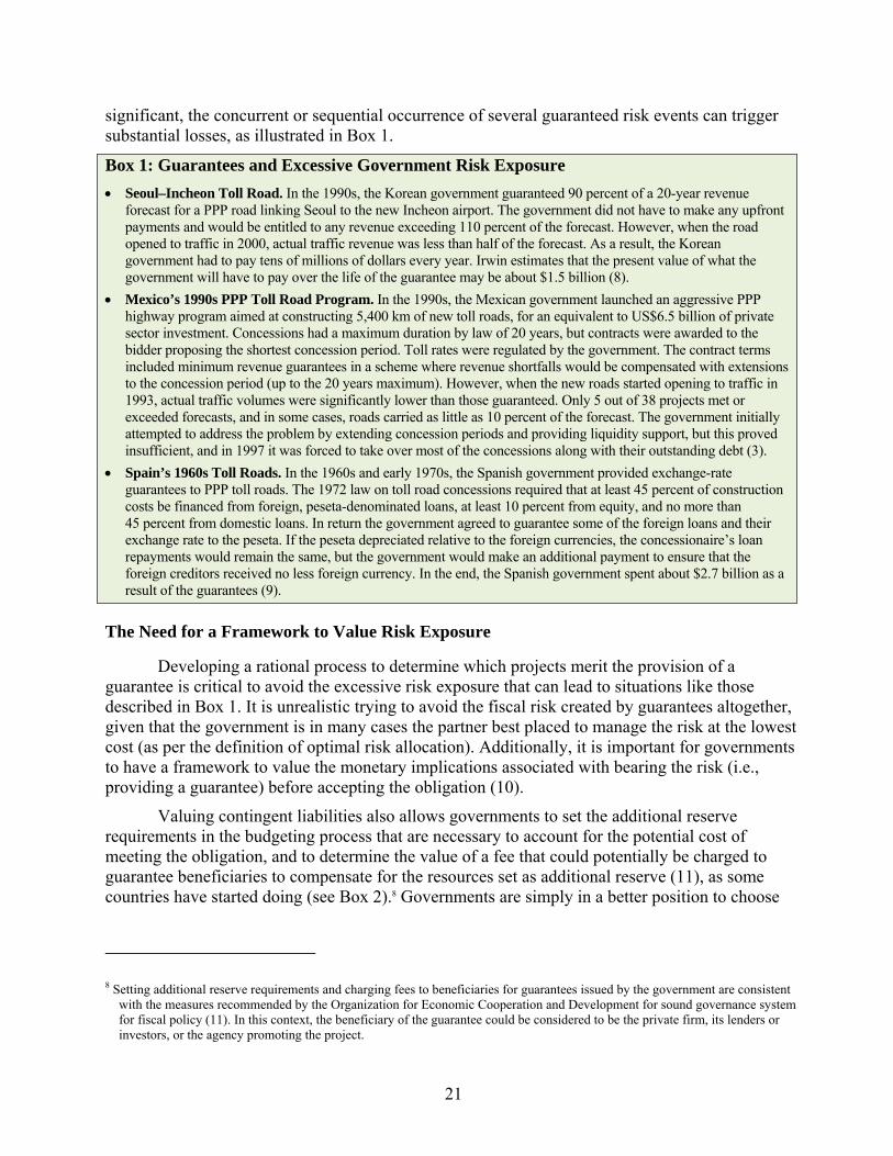
significant, the concurrent or sequential occurrence of several guaranteed risk events can trigger substantial losses, as illustrated in Box 1.

Box 1: Guarantees and Excessive Government Risk Exposure • Seoul–Incheon Toll Road. In the 1990s, the Korean government guaranteed 90 percent of a 20-year revenue

forecast for a PPP road linking Seoul to the new Incheon airport. The government did not have to make any upfront payments and would be entitled to any revenue exceeding 110 percent of the forecast. However, when the road opened to traffic in 2000, actual traffic revenue was less than half of the forecast. As a result, the Korean government had to pay tens of millions of dollars every year. Irwin estimates that the present value of what the government will have to pay over the life of the guarantee may be about $1.5 billion (8).

• Mexico’s 1990s PPP Toll Road Program. In the 1990s, the Mexican government launched an aggressive PPP highway program aimed at constructing 5,400 km of new toll roads, for an equivalent to US$6.5 billion of private sector investment. Concessions had a maximum duration by law of 20 years, but contracts were awarded to the bidder proposing the shortest concession period. Toll rates were regulated by the government. The contract terms included minimum revenue guarantees in a scheme where revenue shortfalls would be compensated with extensions to the concession period (up to the 20 years maximum). However, when the new roads started opening to traffic in 1993, actual traffic volumes were significantly lower than those guaranteed. Only 5 out of 38 projects met or exceeded forecasts, and in some cases, roads carried as little as 10 percent of the forecast. The government initially attempted to address the problem by extending concession periods and providing liquidity support, but this proved insufficient, and in 1997 it was forced to take over most of the concessions along with their outstanding debt (3).

• Spain’s 1960s Toll Roads. In the 1960s and early 1970s, the Spanish government provided exchange-rate guarantees to PPP toll roads. The 1972 law on toll road concessions required that at least 45 percent of construction costs be financed from foreign, peseta-denominated loans, at least 10 percent from equity, and no more than 45 percent from domestic loans. In return the government agreed to guarantee some of the foreign loans and their exchange rate to the peseta. If the peseta depreciated relative to the foreign currencies, the concessionaire’s loan repayments would remain the same, but the government would make an additional payment to ensure that the foreign creditors received no less foreign currency. In the end, the Spanish government spent about $2.7 billion as a result of the guarantees (9).

The Need for a Framework to Value Risk Exposure

Developing a rational process to determine which projects merit the provision of a guarantee is critical to avoid the excessive risk exposure that can lead to situations like those described in Box 1. It is unrealistic trying to avoid the fiscal risk created by guarantees altogether, given that the government is in many cases the partner best placed to manage the risk at the lowest cost (as per the definition of optimal risk allocation). Additionally, it is important for governments to have a framework to value the monetary implications associated with bearing the risk (i.e., providing a guarantee) before accepting the obligation (10).

Valuing contingent liabilities also allows governments to set the additional reserve requirements in the budgeting process that are necessary to account for the potential cost of meeting the obligation, and to determine the value of a fee that could potentially be charged to guarantee beneficiaries to compensate for the resources set as additional reserve (11), as some countries have started doing (see Box 2).8 Governments are simply in a better position to choose

8 Setting additional reserve requirements and charging fees to beneficiaries for guarantees issued by the government are consistent

with the measures recommended by the Organization for Economic Cooperation and Development for sound governance system for fiscal policy (11). In this context, the beneficiary of the guarantee could be considered to be the private firm, its lenders or investors, or the agency promoting the project.

22

whether to bear a risk if they have measured and valued their prospective exposure—that is, if they have described it quantitatively and estimated its cost (8).

Box 2: Charging for Guarantees While it has been common that the guarantees provided by governments to the private sector in PPPs do not carry any fee with them, the absence of fees on guarantees gives an incentive to the private sector to request all possible guarantees to cover any unexpected losses. Some governments (e.g., India and Korea) have started charging guarantee fees to beneficiaries to compensate for the cost of the resources committed—the additional capital set aside as a contingent liability reserve (12; 13). Some authors suggest that such a charge could be set equal to the estimated value of the guarantee (i.e., the contingent liability), plus a premium to cover the government’s administrative costs (8; 14; 11). Irwin also argues that if the beneficiary is charged, it would compare the price with the benefits of the guarantee and decide whether the guarantee is worth taking, reducing the probability of the government’s issuing guarantees less valuable to the beneficiary than they are costly to the government (8).

23

CHAPTER 3: PUBLIC RISK IN INFRASTRUCTURE PPPs—INTERNATIONAL

PRACTICES AND LESSONS LEARNED

The objective of this chapter is to validate the argument for a more systematic approach to valuing public sector exposure in U.S. PPPs, one that is based on tried and tested features from different approaches used internationally. The first section of this chapter provides an overview of the current U.S. practices, reviewing several recent high-profile U.S. PPP transactions, summarizing some of the salient risk-sharing features of each one, particularly regarding how public agencies dealt with those risks they retained in each case. The second section reviews the experiences of several countries known for having developed formal approaches to deal with PPP explicit public sector risk exposure (i.e., guarantees) and examines their risk valuation practices. The third section condenses the lessons learned from the international experience and identifies common features in their public sector risk exposure management approaches that could be adapted to improve current U.S. public sector PPP practices.

DEALING WITH PPP PUBLIC SECTOR RISK EXPOSURE IN THE UNITED STATES

Under the U.S. federal system of government, most transportation infrastructure development falls within the responsibility of state governments; similarly, policies to engage the private sector in transportation infrastructure development have largely been developed at the state level. Despite the fact that these policies are a relatively recent trend among U.S. states, a number of high-profile PPP transactions have taken place since 2005, particularly in Texas, Illinois, Indiana, and Virginia. Since traditional transportation funding constraints are unlikely to disappear anytime soon, it is very likely that this trend will only increase in the near future.

There are many lessons learned from the transportation PPP projects that have been implemented to date in the U.S. In February 2008, the U.S. Government Accountability Office (GAO) released a report to Congress entitled Highway Public-Private Partnerships: More Rigorous Up-Front Analysis Could Better Secure Potential Benefits and Protect the Public Interest, which reviewed the U.S. recent PPP experience. Although the report noted the significant benefits of PPPs, its main focus was on the risks, costs and tradeoffs that come along with private sector participation (15).

The report recognizes the systematic approaches that other countries have developed to identify and evaluate public sector interest (including risk) in PPPs, such as the VfM and the PSC concepts, and the limited use of such approaches in the U.S. Furthermore, recognizing that the PPP trend will continue in the future, the report concludes that there is a pressing need to develop and formally implement similar systematic approaches by U.S. transportation agencies.

This section presents four recent high-profile PPP transactions, describing the most significant features of each project and highlighting some of the most relevant risk allocation arrangements, indicating to what extent there has been a systematic or formal effort to evaluate public sector risk exposure. The cases presented are from the states of Texas, Illinois, and Indiana. One of the Texas cases is the controversial SH 121 project, in which a public agency was awarded the project over a private firm.

24

Texas Sam Rayburn Tollway

The need to reduce the growing congestion in Texas led to enactment of state legislation in 2003 to expand the use of innovative financing mechanisms, including tolling and PPPs by the Texas Department of Transportation (TxDOT).9 The legislation enabled TxDOT to commence a program to attract private investment to develop additional capacity on the state’s most congested corridors. One of these projects is the State Highway (SH) 121 Tollway (or Sam Rayburn Tollway), a toll facility to be built as the main lanes of SH 121, which stretches 26 miles through the counties of Collin, Dallas, and Denton.

In February 2007, a consortium led by the Spanish firm Cintra and TxDOT agreed to a US$2.8 billion, 50-year comprehensive development agreement (CDA) to build, operate, and maintain the Sam Rayburn Tollway. The consortium’s offer included a US$2.1 billion upfront payment and a series of annual payments with a present value (PV) of US$700 million; however, the project had become highly controversial in the run-up to the conclusion of the procurement process, as significant opposition to tolling and private sector participation in highway infrastructure developed in the North Texas region, and indeed throughout the state. Opponents of the agreement with Cintra had been questioning the length of the agreement and the fact that the North Texas Tollway Authority (NTTA), a public toll road operator, had been prevented from bidding on the contract after TxDOT had received complaints from private bidders. In response to the opponents to the agreement with Cintra, state legislators pressed the department to accept a proposal from NTTA (16).10

NTTA submitted its bid in May 2007, offering to pay TxDOT approximately US$3.3 billion (a US$2.5 billion upfront payment, and annual payments with a PV of US$833 million), a significantly higher amount than the private sector proposal. However, it is important to note that this bid was based on traffic forecasts and other key assumptions that were different from those used by Cintra.

A document published by NTTA recounting the history of the toll road states that their May 2007 proposal for the Sam Rayburn Tollway was prepared as a “public sector comparator” (17). However, the economic benefit analysis comparison presented by NTTA in its proposal and illustrated in Figure 5 does not indicate that adjustments were made for the cost of the risk 9 In 2003, the Texas 78th State Legislature passed HB 3588 on the Trans-Texas Corridor and retooling transportation project

finance. The bill integrated existing and recent transportation policies with new initiatives and financing mechanisms designed to accelerate project delivery and to generate additional cash flow to fund transportation projects, including tolling and PPPs. The text of the enacted bill can be found at http://www.legis.state.tx.us/tlodocs/78R/billtext/pdf/HB03588F.pdf#navpanes=0.

10 This controversy also led to the Texas State Legislature passing Senate Bill 792 in 2007, which requires conducting a process called market valuation. The market valuation process basically consists of developing “shadow bids” for highway PPPs that are used as benchmarks to accept proposals from local public tolling entities, which under the legislation have the right of first refusal to develop a toll project, before TxDOT can solicit proposals directly from the private sector (see Box 9 for more on market valuation). These shadow bids include detailed estimates of design, construction, and operating costs and a financial model, the results of which are compared against private sector proposals. The 2008 GAO report argues that Texas has used these shadow bids as a proxy to a PSC. The report also states that while there are no statutory or regulatory provisions defining the public interest in PPPs. When procuring PPPs, TxDOT develops specific evaluation procedures and criteria for each specific procurement, as well as contract provisions that are determined to be in the interest of the state. PPP proposals the department receives are then evaluated against those project criteria. However, these criteria are project-specific, and there are no standard criteria that are equally applied to all projects (15). Moreover, neither these approaches nor the market valuation process itself includes a monetary valuation of risk, leaving a fundamental part of the VfM concept of the PSC concept totally unaddressed.

25

retained by the public agency, and which the private concessionaire would have otherwise borne. In other words, the analysis was biased against Cintra by not adding to its proposal the cost of risk bearing as an economic benefit to the public.

Figure 5: Sam Rayburn Tollway Economic Benefit Comparison—NTTA vs. Cintra (18)

Texas State Highway 130 Segments 5 & 6

A second recent example from the TxDOT PPP program is SH 130 segments 5 and 6. SH 130 is a toll road in Central Texas that once completed will form a 91-mile corridor from Interstate 35 (I-35) in Georgetown (north of Austin) to I-10 near Seguin. The corridor runs parallel to I-35 between Austin and San Antonio, providing relief to this congested corridor. Segments 5 and 6 of SH 130 form a 40-mile link through the counties of Travis, Caldwell, and Guadalupe.

In June 2006, TxDOT and a consortium formed by Cintra and Zachry American Infrastructure (a Texas-based firm) agreed to a 50-year CDA to finance, design, build, operate, and maintain the 40-mile project. The offer from Cintra-Zachry for the US$1.35 billion project included an upfront payment of US$25.8 million and the prospect to share in the revenue and savings resulting from refinancing concessionaire-issued debt. The revenue-sharing provisions are laid out in seven pages of tables with three different toll revenue-share rates (from 4.65 percent through 50 percent), with thresholds rising year by year and the revenue rates depending on the posted speed limits (19).

According to TxDOT, all project risks were identified and allocated following the basic principle of allocating risks to the party best able to manage them. The risks allocated to Cintra-Zachry included financing, design, construction, right of way acquisition, hazardous material

26

costs, permits and approvals (except environmental), environmental mitigation costs, normal force majeure (labor disputes, adverse weather, floods, earthquakes, etc.), operations and maintenance, and traffic and revenue (20). TxDOT, however, indirectly retained part of the revenue risk. For example, the agreement includes non-compete clauses to compensate the concessionaire in the event of the speed limit being raised on I-35 or in case a competing facility that might compromise the toll road revenue is constructed. Also, TxDOT retained toll collection risk, as it applies to users who do not have an electronic toll tag in their vehicle and might refuse to pay. TxDOT plans to mitigate this risk by charging a toll premium to those users (who are identified by a video toll matchup system) and using the premium to compensate for those tolls that cannot be collected (21).

Although this risk allocation is reportedly the most advantageous TxDOT had ever obtained until then (20), no formal procedure or methodology was used to estimate the monetary cost of bearing the risks.

Indiana Toll Road

The 157-mile long Indiana Toll Road (ITR) has been in operation since 1956 when it first opened to traffic providing a main highway link between the Midwest and the East Coast. The Indiana Department of Transportation operated and maintained the ITR for 25 years until 2006 when the toll road was considered for lease (22). With the ITR open for bidding in January of 2006, the joint venture between a consortium formed by Cintra and Macquarie Infrastructure Group (Australia) made an offer for US$3.85 billion that easily surpassed any competing bids (Babcock & Brown offered the next highest bid of US$2.84 billion). As a result, the state of Indiana and the Cintra-Macquarie consortium signed a 75-year concession agreement starting in 2006 and concluding in 2081.

As with any other PPP agreements, the public and private partners share project risks. For example, floods in Indiana (September 2008) caused damages to several highways, forcing the state to close them down and detour traffic. During these events, the ITR was temporarily used as a toll-free highway to alleviate congestion in surrounding areas that had been affected by the floods. The flood cost the state an unknown amount of money because the Cintra-Macquarie consortium eventually demanded to be reimbursed for the traffic that did not pay for using the highway during the flood (23). The state planned to compensate the consortium from the US$3.85 billion lease agreement payment received; however, the actual compensation amount paid was unknown.

Part of the concession agreement also included that Cintra-Macquarie would be compensated for any road upgrades done by the state that could potentially reduce the income from the toll road. The road upgrade clause refers to any new comparable highway that has a minimum length of 20 miles and is located within 10 miles of the ITR (24). Furthermore, if the state decides to take action in which those previously mentioned conditions are met, then the government will have to monetarily compensate the consortium. Eventually, the need for transportation infrastructure will likely become a necessity in the area during the 75-year concession period, triggering the guarantee. However, no evidence was found of a quantitative analysis of the monetary value of this contingent liability. The GAO report further confirms that Indiana did not develop a public interest test or a PSC prior to the transaction.

27

Chicago Skyway Toll Road

In the state of Illinois, the Chicago Skyway Bridge toll road has served as an important roadway that connects the ITR to the Dan Ryan Expressway located on the Southeast side of the city. The 7.8-mile toll bridge had been operated by the City of Chicago Department of Streets and Sanitation for almost 50 years, from 1958 to 2004, when the city of Chicago called for bids from private sector developers for the right to operate the toll road. As in the ITR case, the winning bidder was the Cintra-Macquarie consortium (25). The consortium offered an upfront payment of US$1.82 billion for the right to operate the Chicago Skyway for a period of 99 years (from 2005 to 2104).

The lease agreement between the City of Chicago and the Cintra-Macquarie consortium was signed in January 2005. Under the agreement, Cintra-Macquarie can increase tolls by a maximum amount of 7.9 percent per year from 2008 through 2017, a series of substantial increases. Unlike the case of the ITR, the Skyway agreement does not contain any clauses that prevent the government from constructing competing facilities. However, the steep toll rate increases built into the agreement may deter a significant amount of commuters from using the Skyway (26). This traffic would likely divert to other city streets, significantly increasing the operations and maintenance costs of those roadways.

Using proceeds from the transaction, the City of Chicago created an emergency reserve fund of US$500 million intended to hedge expenses related to the now-leased Chicago Skyway among other things (27). However, there is no evidence that the fund amount was established as a result of an estimation of the project’s contingent liabilities, or as part of a formal risk analysis protocol.

INTERNATIONAL EXPERIENCE DEALING WITH PPP PUBLIC SECTOR RISK EXPOSURE

Along with the increasing popularity of PPPs, there has been a general international increase of interest in managing public sector risk exposure in PPPs, particularly as it relates to contingent fiscal liabilities. International standards increasingly require disclosing these liabilities in public accounts, and countries are introducing new approaches to managing and controlling their exposure. However, there is still relatively limited international consensus on managing fiscal risk specifically arising from PPP projects in infrastructure. Governments seeking to manage their exposure to risk from guarantees to infrastructure PPPs have done so in a number of ways, reflecting their specific objectives and institutional strengths or limitations.

It is nonetheless useful to consider the experiences from other countries in managing and valuing public sector risk exposure in PPPs. Therefore, lessons learned from tried-and-tested common features, and the analysis of what drives the differences that exist, are one of the key inputs in this research to develop a framework that can be applied to value public sector risk exposure in PPP projects in the U.S.

This section documents current international practices for the management of public sector PPP risk exposure, particularly as it relates to valuation of contingent liabilities resulting from risks retained by governments. There are public sector risk management frameworks in place or under development in several countries throughout the world that incorporate several key functions, including the definition of a standard approach to valuing risk exposure through

28

contingent liabilities. Although the specific mechanisms used to implement these functions differ between countries, some principles remain common. The following sections present case studies from four countries with successful PPP programs: Colombia, South Africa, Chile, and the State of Victoria, in Australia.

Colombia

During the 1990s, the Government of Colombia issued guarantees for a wide variety of risks in respect to electricity, roads, and telecommunication PPP projects. The value of the contingent liabilities to the government from having issued these guarantees was estimated at around 1.5 percent of the country’s gross domestic product (GDP) in 1997. At that time, the general consensus was that guarantees were issued indiscriminately by implementing government agencies. There were no rules on how to decide whether to issue a guarantee or not, or on how to cover the government’s exposure from these guarantees. As result, many guarantees were offered to poorly structured projects in which the government was bearing an excessive amount of risk.

Between 1998 and 2003, the Government of Colombia defined new rules and procedures for issuing PPP-related guarantees, with a series of laws, decrees, and policy documents. The primary objective of these was to manage the fiscal risks associated with future guarantees.

Overview

The provision of guarantees in Colombia is now controlled by the Risk Management Unit (RMU) in the Ministry of Finance (MoF). This unit is responsible for assessing and approving guarantee requests prepared by implementing institutions, according to well-specified criteria of acceptable risks. Budget provisions against guarantees are made by transfers from the implementing institution to a contingency fund, a special government account that is managed by a private financial institution.

Projects and Risks

Risks that the government was prepared to guarantee were clearly defined, based on the principle that risk should be allocated to the party that is best placed to value and control the risk, and that has best access to mitigation, protection, and diversification instruments. For each infrastructure sector, the government defined the specific risks that it was prepared to bear or share, as well as the mechanisms that should be used for mitigation. For example, for a toll road project, the government is only prepared to bear land acquisition risk. Traffic demand risk is borne by the concessionaire, but shortfalls are dealt with by extending the term of the contract until the concessionaire achieves a pre-agreed level of expected revenue, avoiding a fiscal cost.

Policies for Valuing and Managing Guarantees

In preparing and approving claims and managing the contingency fund, the government and contracting private financial institution are guided by policies designed to manage the fiscal risk of providing guarantees:

• Guidelines for calculating the value of the contingent liabilities—that is, the present value of the expected cost of the guarantee to the government— require

29

the use of risk-pricing modeling methods such as Binomial trees or Monte Carlo simulations (see example in Box 3)

• Mandating the implementing institutions to make transfers to the contingency fund equal to the expected value of the guarantee ensures the expected value of the total stock of guarantees does not exceed the assets of the fund. These transfers are made up front and may be topped up over time if the expected value of the guarantee changes.

The contingency fund holds a separate account for each project, funded by the transfers from the implementing institution. In the case of a payment claim, any shortfall is met by the government institution that is party to the PPP contract.

South Africa

South Africa commenced its PPP program in the late 1990s, and in 2000, its National Treasury established its PPP Unit. The program started with two toll roads, two jails, retail concessions in national parks, and power plants. Later, the program incorporated PPPs for

Box 3: Valuation of PPP Contingent Liabilities in Colombia (28) In 1996 the Colombian government and the World Bank worked together to quantify the risk exposure of three project finance transactions. The collaboration made it possible to establish a framework to value the government’s risk exposure. The study used a sophisticated contingent valuation methodology incorporating Monte Carlo simulation to value the contingent liabilities associated with three infrastructure projects, among which the El Cortijo-El Vino toll road project was included. The other two infrastructure projects included in the analysis were a telecommunication joint venture (Telecom-Siemens) and an energy sector project (CORELCA). The first step was to identify all of the risks associated with each of the projects. In addition, the exchange rates and demand volumes were assumed to follow a correlated lognormal process. Moreover, the variance estimates were calculated by examination of the variability of cash flows for each of the projects involved in the analysis. Once these estimates were made, the team employed stochastic analysis to obtain the net expected losses for each of the projects. The team also analyzed different types of risk and how bearing these specific risks impacted the government. For example, the El Cortijo-El Vino toll road project’s largest risks were identified to be traffic demand volatility and construction risks. The analysis showed that the Colombian government could lose up to US$4.2 million from those two guarantees. The team finally came up with expected losses after employing the contingent claims analysis method to value the government’s exposure. The table below shows the resulting expected losses from the three different infrastructure projects analyzed.

Type of risk El Cortijo-EI Vino Toll

Road Project (US$’000)

Telecom-Siemens Joint Venture

(US$’000)

CORELCA Energy Guarantees

(US$’000)Market risk 3,100 2,500 52,000Construction risk 1,100 9,800 0Counterparty risk 250 100 5,000Currency risk 0 -1,300 2,000Force majeure 200 300 7,000Termination risk -150 200 1,000Regulatory risk 0 10,100 0

Total 4,500 21,700 67,000

30

hospitals and health services, government office buildings, government vehicle fleets, and the Gautrain, a new railway linking Pretoria and Johannesburg (29).11

Overview

In South Africa, the public agency’s largest contingent liability in most PPP contracts is an obligation to compensate the private firm if the contract is terminated before its scheduled end. On the other hand, in case of the private firm’s default, the required compensation may be a prearranged fraction of the outstanding debt, if the outstanding debt is greater than the market value of the project. In other words, the government may bear some of the losses associated with the private firm’s default, along with shareholders and creditors.

PPP proposals and their associated contingent liabilities follow a four-stage process to be approved by the National Treasury. The objective of the first stage is to demonstrate that the public agency can afford the PPP and obtain for the project the first level of approval (called Treasury Approval I). In this stage, the public agency registers the project in the process and appoints a project officer and transaction advisors, who then perform a feasibility study. The objective of the second stage is to demonstrate VfM and secure Treasury Approval II. The second stage includes the preparation of project procurement documentation, while the third stage includes the bidding process and selection of a preferred bidder. The objective of the fourth stage is to reach financial closure and includes the negotiation of the final PPP agreement and final review by the Treasury’s fiscal liability committee.

Selection of Risks

South Africa has a standardized PPP contract provisions document that discusses the provisions that should be in PPP agreements. Among other things, the document defines in some detail the provisions that should govern early contract termination and associated compensation payments. Therefore, the document plays a key role in controlling the contingent liabilities that the public sector assumes in a PPP. The National Treasury PPP Manual also includes a detailed standardized PPP risk allocation matrix that defines the risks that the public sector is willing to retain (30).

The process for developing PPPs entails a number of analyses relevant to the management of contingent liabilities. The first one is a cost-benefit analysis for major transportation projects, which is noted not only in the PPP Manual but is also referred to in the Public Finance Management Act of 1989. The second analysis is part of the feasibility study required for Treasury approval, where departments considering a PPP must carry out a PSC analysis, comparing the costs and benefits of a PPP with the costs and benefits of a publicly financed project. Detailed guidance for this analysis is provided in the PPP Manual (30). The approach to the PSC is partly based on practice in Australia and the United Kingdom.

11 For a more thorough discussion of South Africa’s PPP program and contingent liabilities, the reader is referred to Irving and

Mokdad (29), from which this material has been summarized.

31


In its PSC analysis guidance, the PPP Manual includes a thorough analysis of risks borne by the government. The estimated costs of both the PSC and the PPP option must include the expected discounted cost to the public agency of the risks it bears. For the PSC, the underlying assumption is that there are risk-related costs that the government bears in a traditional publicly financed project, but they are seldom quantified. An example of this would be construction cost estimates that may not fully account for probable delays and budget overruns. The risk-adjusted PSC is intended to remedy this problem by adding to the “base” public-sector comparator an estimate of the expected cost overrun in the form of probability-weighted average of estimated costs associated with different scenarios. For the PPP option, the concept in the analysis is that the private firm will not bear all project risks; therefore, estimating the full cost of the PPP requires estimating not only the costs for which the private firm will charge but also the additional risk-related costs that the government will bear.

Box 4: Valuation of PPP Contingent Liabilities in South Africa (29) The Gautrain is an example of a PPP project in South Africa where the project company gets its revenue mainly from user fees, and where the public sector has also assumed contingent liabilities related to user demand. In this case, the provincial government will pay the private firm the difference between its actual revenue and a predetermined minimum level, if actual revenue is below the predetermined minimum but more than the concessionaire’s revenue forecast. The minimum revenue level is an estimate of the revenue the concessionaire needs to cover all its costs, including the cost of capital. It exceeds forecast revenue by some 360 million South African rand a year (about US$51.8 million). The Gautrain’s PPP Treasury Approval III report included a 50-page report on the contingent liabilities created by the revenue guarantee for the Gauteng province. The report described the liabilities, explained the logic behind the contractual provisions that created the liabilities, and discussed their magnitude. In some instances, the report (justifiably) declined to estimate the probability of payments or their expected value. In other cases, it quantified the maximum payments and gave rough estimates of expected payments. For example, the analysis of the possible cost of the user demand (revenue) guarantee used Monte Carlo simulation to estimate the probability distribution of the payments to be made by the government.

Chile

Chile began its PPP program in the early 1990s with highway concessions. The Concessions Law was passed in 1991, and the concessions program began in earnest in 1994. Chile’s concession program now includes highways, airports, jails, and other types of public infrastructure (such as stadiums and transit stations). The Government of Chile offers guarantees that focus mainly on traffic levels in transportation PPPs. Its goal is to reduce the risk profile of a given project in which investment decisions made by the government could lower the project’s cost of capital and thus the total cost of the project. The government is in a strong fiscal position and has been one of the best performing economies in Latin America since before 2000. Chile’s framework for managing the fiscal risk of government guarantees reflects its sound fiscal position and is geared toward minimizing and monitoring the fiscal implications of guarantees.

Overview

Chile’s framework for managing government guarantees to infrastructure projects centers around carefully structuring guarantees to limit the government’s exposure, and valuing and monitoring the contingent liabilities that arise from these guarantees. In 2003, the government instituted a policy for valuing, reporting, and monitoring all of its contingent liabilities. This

32

includes not only guarantees to infrastructure projects but also to the debt of state-owned companies, financing for higher education, and minimum pensions.

The government—through the Ministry of Public Works (MPW)—is currently party to concessions for 22 inter-city highway projects, 7 urban highway projects, 10 airports, 2 jails, and several other public buildings. All but three of the inter-city highway projects, and most of the airports, have a minimum revenue guarantee. Only two urban highways have a minimum revenue guarantee.

The value of the contingent liabilities associated with guarantees to infrastructure PPPs has been very low since the policy of valuing and reporting them began in 2003. Their value has fluctuated between 0.15 and 0.25 percent of GDP, or approximately 0.3 to 0.8 percent of the government’s annual budget. The present value of the future payments under guarantees to infrastructure PPP projects at the end of the 2009 fiscal year was US$342 million.

Projects and Risks

There are no formal rules regarding the types of risks that the government may accept through guarantees, or the projects that it may provide guarantees to. However, a clear project evaluation process is designed to ensure guarantees provide value for money. All public investment projects—including infrastructure PPPs—are subject to a thorough evaluation involving the MPW, the Ministry of Planning and Cooperation, MoF, and the Comptroller General. The objectives of this evaluation are to ensure that projects do the following: a) are consistent with the government’s national infrastructure plan; b) pass a social cost-benefit analysis; c) are undertaken by the public or private sector, depending on which is best placed to carry them out; and d) are acceptable from a macroeconomic and fiscal sustainability perspective (31). The MoF must also approve the procurement documents of any PPP contract before it goes to bid. The terms of any proposed guarantees are included in these documents. The Contingent Liabilities, Guarantees and Concessions Unit (CLGCU) in the MoF is responsible for reviewing and approving these guarantees.

Most of the guarantees provided in Chile to date have been minimum revenue guarantees for projects in which decisions made by the government have a significant effect on the revenues (e.g., toll roads).12 For these guarantees, companies bidding on a PPP project could choose whether or not to accept the guarantee offered in the procurement documents. If they chose to accept it and won the project, they were also required to make a payment to the government equal to the present value of the expected cost of the guarantee, as measured by the government.

Under more recent toll road PPPs, the Chilean government has moved away from providing minimum annual revenue guarantees, instead adopting variable-length contracts. Under this approach, the concessionaire’s required NPV of revenue over the project lifetime is the bid criterion in the tender process. The contract length varies to achieve this total level of revenue. This approach avoids creating a contingent liability for the government.13 A similar 12 Guarantees against currency devaluation were provided by the Chilean government until 2005. In these guarantees, both down-

side and up-side risks were shared with the private sector. Development of the domestic capital market has since allowed concessionaires to raise peso-denominated debt, obviating the need for these guarantees.

13 The variable length contract approach also means the timing of re-concessioning (and rehabilitating or expanding) the road responds to the level of traffic experienced.

33

approach, limiting the government’s fiscal exposure, is taken with termination payment clauses. The Chilean government typically offers a termination payment guarantee, should the project company default on its obligations. However, the payment is conditional on the government re-tendering the concession and set equal to the price obtained—this therefore also creates no contingent liability for the government.


The Chilean government’s system for managing its exposure to risk from contingent liabilities focuses on structuring its guarantees well to minimize fiscal risk and on valuing and reporting its exposure. Although payments on government guarantees come from line ministries, the government’s net exposure from minimum revenue guarantees is offset by the initial payment made by the concessionaire.14 The CLGCU of the MoF uses a spreadsheet model to value the government’s contingent liabilities using stochastic analyses through Monte Carlo simulations to measure the risk associated with the risk factors underlying the guarantees, and then uses the Black and Scholes method to value the guarantees (see Box 5).

Box 5: Valuation of Contingent Liabilities in Chile (29) The first part of the spreadsheet model used by the MoF in Chile is a mathematical representation of the clauses of a concession contract concerned with revenue guarantees and revenue sharing in a spreadsheet. The essence of the revenue guarantees is simple: if actual traffic revenue exceeds the guaranteed level, the government pays nothing; otherwise, it pays the difference between actual and guaranteed traffic revenue. The guarantee can thus be modeled by using “if–then” or maximum functions. Some of the revenue-sharing (or more accurately profit-sharing) provisions are more complicated. The second part of the spreadsheet is a model of traffic revenue for each of the roads and airports with revenue guarantees. For each concession in operation, the projection starts with actual revenue of the previous year. Estimates of expected growth may come from traffic forecasts, if they are recent and still considered useful, or from forecasts of GDP and an estimate of the income elasticity of traffic revenue. Randomness is incorporated by assuming that traffic revenue evolves as a geometric random walk with growth. The geometric aspect of the random walk means that rates of growth and volatility of revenue are assumed to be proportional to current revenue. The expected growth rate can change from year to year, as well as differing from concession to concession. The rate of volatility is assumed to be the same for all years and all roads. The main source of the estimate of volatility is historical variation in revenue on roads that have been open for a few years. A rough estimate of the correlations among the revenues on different roads is also incorporated in the model. Chile’s concessions have been operating for many years, and there were public toll roads before there were private concessions, so historical data are plentiful. For roads that have not yet been opened to traffic, initial revenue is treated as a random variable. The random variable is assumed to have a lognormal distribution, which means that initial revenue cannot be negative. To account for optimism, the mean of the random variable is allowed to be lower than the forecast of revenue prepared when the concession was developed. These two parts of the spreadsheet model estimate the frequency distribution of payments by and to the government in each future year of each concession. In most cases, the frequency distributions are derived from Monte Carlo simulation. The third part of the model estimates of the value of the government’s right to receive possible revenue-sharing payments and its obligation to make possible guarantee payments. The spreadsheet model prices the risk of revenue guarantees and revenue-sharing arrangements by estimating risk-adjusted expected payments, or certainty equivalents. The certainty equivalents are then discounted at the risk-free rate to get present values.

14 The government has considered establishing a guarantee fund for infrastructure PPPs. However, because the value of the

contingent liabilities in relation to GDP and the government’s budget is so small, the government has determined that the benefit of establishing this fund would be minimal.

34

Victoria, Australia

The State of Victoria’s PPP program is one of Australia’s best known. Since the State introduced the program in 2000, 16 projects have been successfully implemented. The PPP program’s stated primary objective is achieving VfM in public expenditure on infrastructure.

Overview

The Victorian government’s comprehensive management framework for PPPs—called “Partnerships Victoria”—aims, inter alia, to ensure that the risks the government undertakes through PPP projects are justified and provide good VfM. The Partnerships Victoria framework was outlined in a policy document and has been periodically updated with the publication of implementation guides (32). The Partnerships Victoria approach and guidance material has since formed the basis of the PPP framework for other Australian states and of a national PPP framework (33).

Risk and Project Selection

The main thrust of the Partnerships Victoria policy is the definition of those risks the government will accept in relation to PPP contracts. The initial policy document laid down the principle that, after pre-supposing that the private party bears all project risks, the government should “take back” those risks it can manage at lower cost. Two further principles were also established: a) whoever is allocated risk must have the freedom to choose how to handle and minimize it; and b) the materiality of the risk should be a consideration in its allocation.

The government set out its initial approach to the allocation of each type of PPP project risk in the Risk Allocation and Contractual Issues Guide, issued in 2001. This guidance was updated in 2005, when the government published the Standard Commercial Principles Guide, which currently acts as a basis for all PPP contracts. This guide includes an updated set of risk allocation preferences and defines how these will be reflected in the terms of a PPP contract.


The evaluation process for each PPP project is also clearly outlined in the Partnerships Victoria policy. This involves a quantitative cost-benefit analysis of PPP provision, including the cost of the guarantees incorporated in the PPP contract, in comparison with other alternatives such as public sector provision through a PSC analysis. The Partnerships Victoria policy also provides advice on measurement of risk and how to incorporate it into the PSC analysis to produce a risk-adjusted PSC.

Since most Partnerships Victoria projects are paid for by government departments, rather than users, those payments are known and must be factored into the budget of the relevant department. These kinds of PPP project obligations are reported as part of State debt as “financial leases.” Even for the limited user-pays projects (such as the EastLink toll road), the government has not borne demand risk. This means that in all cases, the risks retained by the government are very limited. The State of Victoria budgets for most of these risks, when quantifiable—which is largely during the construction period—by including an estimated value in the relevant department’s budget.

35

Box 6: Victoria State Risk Valuation Example (Adapted from [32]) The construction of a new hospital project in Victoria, Australia, is being proposed as a PPP. The costs are broken down as shown in the table below:

Category Net Present Cost (AUS$ million) Capital costs 234.60 Operating and maintenance 121.20 Third-party revenue (35.00) Competitive neutrality 15.00 Total not-risk-adjusted PSC 335.80

Using an advanced probability valuation technique based on multivariate analysis, such as Monte Carlo simulation, an artificial probability distribution for total risk is constructed, based on assumed or actual distributions for each of the individual risks. It then provides a single value for risk by simultaneously solving a number of different risk relationships. The results are shown in the table below:

Mean (AUS$ million) % of risk-adjusted PSC Total non-risk-adjusted project cost (incl. competitive neutrality but excl. taxes) 335.80 72

Retained risk 12.80 3 Transferred risk 116.00 25 Total risk-adjusted project cost (excl. taxes) 464.60 100

The costs of risks contained in the table above are mean estimates among a range of possible outcomes. Therefore, it is recommended to focus on the probability distributions generated by the advanced probability valuation technique rather than simply look at the mean result in isolation. For example, analyzing the results is done by looking at the shape of the distribution curves for retained and transferred risk, and for the total PSC minus retained risk. The transferred risk curve is shown in Figure 6, illustrating the mean, as well as the 5th and 95th percentiles. The figure shows that the most frequently occurring value during the simulation is around AUS$100 million, and the mean estimate is AUS$116 million. However, the distribution shows that transferred risk could have a cost impact of around AUS$190 million at the 95th percentile (although with a relatively low probability). These would be the measures of the risk that the public sector would transfer and no longer be exposed to if it were to pursue a PPP.

Figure 6: Transferrable Risk Distribution and Mean—Australia Example (29)

36

LESSONS FROM THE INTERNATIONAL PRACTICE

This section analyzes the commonalities and differences of the risk exposure and contingent liability management frameworks in the different countries examined. This section also examines in particular the lessons learned regarding the use of standard approaches to valuing risk exposure and the applicability of these approaches in the context of U.S. PPPs.

Common Functions and Features of Risk Exposure Management Frameworks

The examples discussed in the previous section illustrate that, despite their largely common principles, there are both similarities and differences between different countries’ systems for managing public sector risk exposure through the provision of guarantees to PPP projects. The different countries’ approaches to risk and contingent liability management are summarized in three functions: 1) defining acceptable risks; 2) setting a standard approach to valuing risk exposure; and 3) defining eligibility criteria or decision rules for acceptable contingent liabilities. These are described in the paragraphs that follow.

1. Defining acceptable risks. Since providing guarantees constitutes a cost to government, most countries seek to ensure this cost is justified. By defining the risks the government is prepared to bear, countries attempt to maximize the benefits from providing guarantees to PPPs. The level of detail to which acceptable risks are defined varies between countries and broadly increases with the country’s level of experience in planning and implementing PPP projects. In Colombia, specific acceptable risks are defined for each infrastructure sector. In Chile, there are no formal rules, but there is strong precedent as to what types of risks and projects have been approved guarantees. In Victoria and South Africa, the acceptable risks, and best methods for allocating these through contract terms, have been laid out in more detail over time in successive policy guides.

This progression may be because in the early stages of a PPP program, the total risk exposure to PPP projects is small relative to the government budget. The government may choose, at this stage, to accept risks beyond those justified by optimal efficient risk allocation in order to attract private investors and build confidence in the PPP program.

2. Setting a standard approach to valuing risk exposure. Of the possible components of a system to manage the fiscal risk arising from government guarantees mentioned above, the one consistently present across countries is a standard approach to valuing contingent liabilities. Whatever risk management structures are in place, they rest on properly valuing the expected cost of the guarantees. This is generally accomplished using option pricing methods and other simulation-based approaches across all countries in the analysis.

Both Chile and Colombia have developed and maintain sophisticated risk-related cost measurement techniques for PPP-related contingent liabilities that are used not only at the project preparation stage but throughout the project lifecycle. Australia and South Africa also do some sophisticated quantitative analysis as part of their PPP project evaluation process. However, as noted by Irwin and Mokdad, determining what level of sophistication and amount of quantification are appropriate depends to a

37

large extent on the nature of the contingent liabilities (29). For example, Chile has several concessions with revenue guarantees that added together create sizeable fiscal risks and that are also similar enough to each other to create economies of scope in measurement and valuation and to justify a level of sophistication. That is, once a revenue guarantee has been quantified, the level of effort to quantify the next one is not as significant. On the other hand, a country with few, small, and diverse PPP guarantees, or cases where the government bears only those risks that it is clearly best placed to manage, may not justify a sophisticated and large effort to measure and value guarantees.

3. Defining eligibility criteria or decision rules for acceptable contingent liabilities. The extent to which the government sets specific decision rules for acceptable contingent liabilities also varies between countries. In Victoria and South Africa, each PPP project is subject to a full cost-benefit analysis in the process of estimating the project’s VfM, which includes a detailed estimation of the cost of providing guarantees. The combination of cost-benefit and PSC analyses provides extraordinarily valuable information for decision makers and can help ensure that government support (through guarantees) is only provided to good PPP projects. However, it is a very complex process, and like any other analytical tools, its outputs are useful only to the extent that they are used to influence decisions (29). That is, if the decision to use a PPP for a particular project has in effect been made before the PSC analysis is undertaken, the value of the analysis will be limited.

Applicability of International Experience to Valuation of Risk Exposure in U.S. PPPs

It can be argued that the three functions identified in the cross-country analysis have direct applicability to the overall recommendation of the GAO report to develop and formally implement a systematic approach to identify and evaluate public sector interest (including risk) in U.S. transportation PPPs. The three functions and the extent of their applicability to the U.S. case studies in the context of this research are discussed below.

1. Defining acceptable risks. While the U.S. examples that were analyzed defined the risks that were acceptable to the public agency for the project in question, the definition of acceptability did not include an associated figure for the cost of risk. The analysis suggests that as U.S. states move toward increased use of PPPs to close the infrastructure gap, policies and guidance that define acceptable risks and best methods for allocating them through contract terms should be developed.

2. Setting a standard approach to valuing contingent liabilities. None of the U.S. examples analyzed followed a standard structured approach to valuing public sector risk exposure. The findings of the analysis, in the context of the increasingly common use of PPPs to fund transportation infrastructure in the U.S., suggest that there is also a growing need to define standard approaches to value public sector risk exposure at the state level, and arguably at the federal level.

3. Defining eligibility criteria or decision rules for acceptable contingent liabilities. The U.S. PPPs reviewed had a clear delineation of the risks that would be retained by the government. However, none of them appeared to have determined the allocation of risk using an approach based on a monetary value of the cost of risk bearing and

38

VfM. The analysis suggests that because of the similarities between the Australian and the U.S. federal structures and transportation planning policies, it would be useful for U.S. states to consider developing and adopting similar policies or guidelines.

Of these three functions, the second one is the most relevant for this research. The rest of this document builds on this argument to develop the risk valuation framework.

39

CHAPTER 4: VALUING PUBLIC SECTOR RISK IN TRANSPORTATION PPP

PROJECTS

The objective of this chapter is to present a methodological framework for the valuation of public sector risk and a step-by-step methodology to measure public sector risk exposure in a transportation PPP project. The first section of this chapter provides an overview of the risk measurement principles and concepts that are used in the risk valuation framework. The second section reviews some of the more common methods employed to value public sector risk using contingent liabilities, such as guarantees, as a proxy for risk exposure in infrastructure projects. The third section describes the methodological framework proposed in this research to value public sector risk in U.S. transportation PPPs and presents a practical step-by-step methodology to apply it.

RISK MEASUREMENT

Measuring and valuing prospective government risk exposure is essential to make informed decisions on whether to bear a risk. Risk measuring is part of risk assessment, the second step of the risk management process described in Chapter 2. This step was defined as the estimation of the likelihood of occurrence and severity of loss of risk events—whether by quantitative or qualitative measures, or a combination of these—and involves describing risk exposure in quantitative terms and estimating its cost. If the risk in question is particularly complex or ambiguous, measurement and valuation may prove too vague or complicated to be useful. If the risk is very small, measurement and valuation may be unnecessary. Nevertheless, approximate measurement and valuation are frequently possible, and if the risk is significant, approximations are better than nothing.

For the purposes of this research, risk will be measured by a mathematical description of the frequency and severity of the variability of the risk, summarized using a probability distribution function (PDF). Probability distribution functions are tools for displaying the uncertainty in a variable. There are a wide variety of forms and types of PDFs, each of which describes a range of possible values and their probability of occurrence. Most people are familiar with the normal distribution, the typical “bell curve.” There are several other PDFs that are used throughout the literature to characterize risk, which include the lognormal, beta, uniform, and triangular distributions (34). Most introductory probability and statistics textbooks describe these functions in more detail.

Most risk quantification has some degree of subjectivity. Much information is needed about a specific variable to know the exact shape of the probability function, and such precise information is seldom known; hence, the shape has to be subjectively determined or assumed. To diminish the necessity for such detailed information, uncertain information can be described in terms of particular summary parameters of the PDF. The most common summary parameters of a PDF are the mean and the standard deviation. The mean (μ) is a measure of central tendency for the variable, and the standard deviation (σ) is a measure of the dispersion of the variable. For a given mean value, the larger the range of the variable is, the larger the standard deviation will be. Hence, all other factors being equal, variables with large standard deviations are riskier than variables with small standard deviations (34). Figure 7 illustrates this concept on a normal PDF

using of tcubic feeprobabilihas a smawords, th

METHO

Tguaranteebe estimaapproachamount iguaranteesettled, b

Continge

Tto estima

the cost of twet of concreteity that the ealler standarhe dashed PD

Figure 7

ODS FOR V

To allow a goe) with the cated, accounh suggested bt would trade’s fair value

between know

ent Liability

The literatureate the marke

• Actuafutureannuatrendsadjustemplogiven metho

wo estimatese). Even thoustimate will

rd deviation DF is less ris

7: Measurin

VALUING G

overnment tocost of other nting for the rby Irwin (8)

de for if it wee, or “the amwledgeable,

y Valuation

e suggests thet value of c

arial or state loss patternal expected los in frequencted loss distroyed to estimyear (36). L

ods fail to ill

s for the cosugh both PDbe on or beland hence h

sky.

ng Risk Usin

GUARANTE

o compare thpolicies, therisk and the to value a g

ere traded. Inmount for wh

willing part

n Methods

hree differentontingent lia

istical methns based on poss distributcy and severiribution remmate the expeLewis and Mlustrate the lo

40

st of a constrDFs have a mlow the US$

higher reliabi

ng Probabil

EES AND C

he cost of bee value of thtiming of thuarantee is tn accountinghich an assetties in an arm

t methods coabilities, suc

hods. The acprevious losstion, and thenity of the expains stable oected and un

Mody (37) recoss patterns;

ruction inputmean of US$$50, the dashility on the p

lity Distribu

CONTINGE

earing a partie guarantee

he governmeto estimate itg jargon, the t could be exm’s length tr

ommonly usech as guarant

tuarial or stas experiencen it is adjustpected losse

over time, thnexpected cocognize the d; consequent

t as an examp50 per unit a

hed PDF is tiprice of the e

ution Funct

ENT LIABI

icular risk (eor contingennt’s possiblets market vaapproach is

xchanged, orransaction” (

ed in the fintees. These m

atistical methes. They apprted accordinges. Assuminge distributio

osts of the prdisadvantagetly, they are

ple (e.g., cosand 50 perceighter, that iestimate. In o

ions

ILITIES

e.g., providinnt liability me payments.

alue, that is, ts to estimate r a liability (35).

ancial indusmethods are:

hods estimatroximate an g to current g that the n can then b

rogram for aes, in that sunot suitable

st of ent s, it other

ng a must

The the the

try :

te

be ny

uch to

41

forecast nonlinear trends (e.g., when the amount of risk shared between the government and the private sector changes over time).

• Econometric methods. In their review for risk quantification, Lewis and Mody (37) suggest that econometrics can be used to illustrate the expected loss distribution of how a program may change over time. Lewis and Mody assert that based on the pattern of fundamental economic or financial parameters, econometrics allow for more dynamic projections in order to forecast nonlinear trends in loss patterns. Econometric models have significantly evolved in the last several years; however, such models require substantial amounts of good-quality data.

• Contingent claims analysis method. Contingent claims analysis (CCA) is another method widely found in the literature. Contingent claims are assets or liabilities whose values at a future point in time are determined by other traded securities. The fundamental theory was first developed to value options on financial assets and subsequently applied to value options on real assets, hence the term “real options.” By relying on simplifying assumptions on risk preferences, these options can be evaluated applying Monte Carlo simulation to a discounted cash flow (DCF) model (14).

The lack of historical data typical of infrastructure projects makes a method based on Monte Carlo simulation, like the CCA, one of the most practical to use. Monte Carlo simulation can estimate the distribution of losses and the carrying PDF for a particular guarantee analyzed. In addition, given a confidence level and a number of iterations (the number of iterations depends on the accuracy desired; however, 10,000 is often used), the maximum possible losses in a project—as well as the price of the guarantee—can be estimated.

Therefore, the remainder of this chapter will focus on using the CCA approach to value public sector risk exposure.

Contingent Claims Analysis Approach to Guarantee Valuation

Contingent claims valuation methods have been extensively used in finance to value loan guarantees. A major example of this is the deposit insurance provided by the Federal Deposit Insurance Corporation (FDIC) in the U.S. CCA usually refers to the general framework for “pricing” or costing out various claims that are contingent on certain triggering events or conditions but are not necessarily linked directly to a tradable security (38). More specifically, Almeyda and Hinojosa (36) describe the CCA approach as a combination of the concept called value at risk (VAR) and stochastic analysis using the Monte Carlo simulation technique. Option pricing is a subset of CCA methods that is associated with pricing financial option products based on an underlying tradable security. This is because contingent liabilities such as guarantees can be regarded as derivatives such as put options.

In a CCA, Monte Carlo simulation is used to approximate the price path of the put option (contingent liability) and to simulate a number of scenarios for the portfolio on a target date. VAR is directly calculated from the distribution of simulated portfolio values. The paragraphs that follow provide additional detail on the VAR approach, option pricing techniques, and stochastic analysis using Monte Carlo simulation.

42

Value at Risk

VAR measures the possible monetary losses in a risky asset or portfolio, which in this case applies to the government’s contingent liability portfolio. Some of the key elements of this approach are:

• a specified level of loss in value, • a fixed time over which the asset’s risk is analyzed, and • the confidence interval.

Given these elements, the VAR for a firm or government can be estimated for a specific asset or for a whole portfolio. The VAR method determines the probability of default and the amount of capital needed in the case where risk needs to be covered. VAR is derived from PDFs that can be drawn either empirically (based on historical data) or by approximating a normal curve distribution, and deriving VAR from the standard deviation. For assets and liabilities that lack extensive historical data, such as infrastructure projects, Monte Carlo simulation can be used to estimate VAR.

This method is often applied in order for the government to create reserve funds. Such funds would give the government the ability to cover any future possible losses while reducing the risk of fiscal crisis. This is because the risk of a portfolio of risk exposures is generally less than the sum of the risks of the component exposures.

Option Pricing Techniques

Option pricing bases its method on the similarities between the guarantees and put options to estimate the expected costs of the contingent liability. A put option gives the right, but not the obligation, to the owner to sell an asset for the face value of the loan before the maturity date. In other words, when the government issues a guarantee to cover a private firm’s loan, the firm’s assets are under a put option. In this case, the holder of the put option (the private firm) could call it whenever the market value of the asset is below the prearranged price. If the put option is called by the private firm, the government has the obligation to accept a given asset with a value below what the government had agreed to pay. In this context, it can be said that the value of the put option is the same as the value of the guarantee that is issued to the private sector. This approach to option pricing is also called structural, as it is based on the private firm’s capital structure as follows:

Value of the firm = Debt + Equity

where the value of the firm and the face value of its debt are F and D, respectively.

Whenever the value of the firm (F) is greater than the value of its total debt (D), the put option will not be called by the private sector, and thus the government will make no payment. This situation implies that the repayment of the whole debt is to be expected by the firm. However, if the debt of the firm is higher than its current value, then the put option will be called and the government will have to respond accordingly. This is illustrated in Table 1, which shows the value of both the risky debt and the put option in the two different scenarios (38). The risky debt represents the value of the risky bond; for example, when the value of the firm is less than the debt, the risky bond is F because the government now holds the assets of the firm.

43

Table 1: Guarantee as a Put Option in Option Pricing Analysis Value of: F>D F<D

Risky Debt D F Put Option 0 D-F

The guarantees granted by the public sector on infrastructure projects can be quantified by running option pricing models such as Black and Scholes and binomial tree:

• Black and Scholes model. The Black and Scholes model, illustrated in Box 7, estimates the value of an option and treats corporate liabilities as combinations of straightforward option contracts, applying the concepts of put option and call option. The put option gives the private firm the ability or option of not repaying the debt at maturity and thus selling the assets to the government (i.e., the value of the firm is less than its total debt). On the other hand, the call option scenario is when the private firm defaults on the loan acquired to pay for the asset, making the lender the asset’s new owner, yet the shareholders have the option to buy the asset back if the debt is fully paid.

Box 7: Option Pricing Models for Infrastructure—Black and Scholes (36) This example assumes a guarantee that covers a minimum income level equal to the debt obligations of a hypothetical infrastructure project, where:

V = Debt + Equity = D + S Value of a Company (1) V = Debt + Income = D + I Value of Project, given that equity equals project cash flows (2) V = MGI + I Debt equals Minimum Guaranteed Income (MGI) (3)

Following the basic relationship between calls and puts, or put-call parity: Value of Call + Present Value of Exercise Price = Value of Put + Value of Share (4); therefore: Value of Call + Present Value of Debt = Value of Put + Value of Income (5)

Where the call is the guaranteed party’s option to buy the project after repaying debt, and the put is the guarantee or an option for the guaranteed party to sell the project in case of default.

By incorporating the concept of MGI, we obtain: Value of option to buy + Present Value of MGI = Value of Guarantee + Value of Income (6)

Parting from this relationship, the call and the put (the option to buy and the guarantee) can be priced using the Black and Scholes formulas:

Call = S0 N (d

1) − Xe−rT N (d

2) = Income

T N (d

1) − MGIe−rT N (d

2) (7)

Put = Guarantee = Xe−rT N (−d2) − S

0 N (−d

1) = MGIe−rT N (−d

2) − Income

T N (−d

1) (8)

Where S0 is the current value of equity (cash flows), N is the standard normal cumulative distribution function , X is

the exercise price, T is the time of realization, r is the risk-free rate of return, and: The value of the guarantee is equal to the difference between the present value of MGI and the actual income perceived at time T, which substituted in the Black and Scholes equations (7 and 8) yields:

If IncomeT > PV of MGI, then N(d1) = N(d2) = 1 and N(-d1) = N(-d2) = 0 Call = S0- X = IncomeT – MGI Put = 0

If IncomeT < PV of MGI, then N(d1) = N(d2) = 0 and N(-d1) = N(-d2) = 1 Call = 0 Put = X - S0- = MGI - IncomeT

d2 = d1 – σ √T

ln(S0/ X ) + (r +1/2σ

2)T ln(Income

T / MGI) + (r +1/2σ

2)T

d1 = = σ √T σ √T

(9)

44

When substituting these results in the put-call parity relationship (Equation 6), the expected value of the call at maturity is: Call = e-rT E[MAX (ST – X1 0)] = e-rT E[MAX (IncomeT – MGI, 0)] (10)

And the expected value of the guarantee (put) at maturity is: Guarantee = e-rT E[MAX (0, X - ST)] = e-rT E[MAX (0, MGI - IncomeT )] (11)

Note that two variables are unknown, Income at time T and its volatility σ. The unique characteristics and nature of infrastructure projects make it very unlikely that historic data will be available to determine a project’s variance (volatility) or the likely upside and downside values of Income at time T. However, a standard deviation (σ) can be approximated from relevant proxies such as regional demand history (e.g., traffic history), past experience of other locations, income elasticity, GDP growth, etc. After calculating the σ, run a Monte Carlo simulation to come up with a PDF of returns whose mean value (μ) would be used as the input for Income at time T.

• Binomial tree. The binomial tree model can handle a variety of conditions because it can model and approach the asset over time as opposed to a specific point. In other words, the income of a specific asset can be estimated at certain time (T), over the life of the guarantee. This approach is based on a risk-neutral valuation principle, which assumes that the expected return from all assets is the risk-free interest rate and that future cash flows can be valued by discounting them at this rate. Box 8 illustrates the approach.

Box 8: Option Pricing Models for Infrastructure—Binomial Tree (36) This example assumes an infrastructure project that is expected to generate, at the end of the year, US$180 million under good economic conditions (Vu = US$180 m) or US$60 million under bad conditions (Vd = US$60). Debt held by the project is US$100 million and matures at the end of the year. A guarantee is offered to provide a US$100 million MGI to cover the project’s debt obligations in case the project cannot do it itself at the end of the year. The risk-free rate of return is 8%. The guarantee can be interpreted as a put option, giving the company the right to “sell” the project’s value and receive the guaranteed amount of US$100 million:

• Under good economic conditions, the guarantee would be worthless (Gu= 0 ) • Under bad conditions, the guarantee would cover the difference between that year’s actual income and the

MGI, so the guarantee would be worth US$40 million: Gd = MGI – Incomed = US$100 m - US$60 m = US$40 m (1)

The underlying asset (IncomeT) can take a value equal to Su with probability p, or Sd with probability (1-p), where u and d are the up or down movements of IncomeT. In a risk-neutral world, the underlying asset will yield a return r (risk-free rate):

E(ST) = pSu + (1-p) Sd = (1+ r); or (2) E(IncomeT) = p Incomeu + (1-p) Incomed = (1+ r) (3) Where:

The risk neutral probability can be estimated as: Therefore the value of the put option or the guarantee is equal to:

As in the Black and Scholes model, two variables are unknown—in this case, Incomeu and Incomed. As it is very unlikely that historic data will be available to determine an infrastructure project’s variance or the likely upside and downside values of Income at time T, the recommendation is to approximate a standard deviation (σ) from relevant proxies such as regional demand history (e.g., traffic history), past experience, GDP growth, etc. After calculating the σ, run a Monte Carlo simulation to develop a PDF of returns whose μ would be used as the input for Incomeu and Incomed at time T.

(1+r) – d p = u – d

(4)

(1+0.08) – 0.6p = 1.8 – 0.6 = 0.4

0.4 × 0 + 0.6 × 40G = 1.08 = 22.2

45

Stochastic Analysis Using Monte Carlo Simulation

The Monte Carlo method permits the stochastic analysis of the impact of changes in all possible combinations of variables that influence the financial outcome of a project. Monte Carlo simulation analysis is generally performed using a spreadsheet computer model that uses random sample techniques to characterize the PDF of each variable. The use of Monte Carlo simulation in a computer model allows structuring all available project information to simulate project cash flows and provide a detailed picture of the magnitude and likelihood of project outcome. After a large number of iterations, the combination of probability distributions for each variable allows developing a PDF of the cash flows and of the project’s financial measures, typically the NPV and the internal rate of return (IRR), as shown in Figure 8.15

Figure 8: Stochastic Analysis Using Monte Carlo Simulation

The Monte Carlo simulation method is an integral part of the CCA approach to value contingent liabilities because it allows the analyst to overcome the data challenges posed by the unique characteristics and nature of infrastructure projects (i.e., historical data is generally unavailable because each project is unique). The Colombian example described earlier in Box 3 illustrates some of the experiences using the CCA approach and Monte Carlo simulation to value infrastructure guarantees. The example claims to be the first time that a sophisticated contingent valuation methodology was applied to government infrastructure projects by the central government (28).

VALUING PUBLIC SECTOR PPP RISK EXPOSURE AS A CONTINGENT LIABILITY

This section describes in detail the methodology proposed in this research to value public sector risk in U.S. transportation PPPs. The methodology builds on the CCA approach, which as

15 For example, if a project has a 25 percent chance of having a NPV larger than US$100,000, this means that, if there were a

great number of similar projects, 25 percent of them would be expected to have an NPV larger than US$100,000.

0.1

0 75 150 225‐75‐150

Net Present Value (‘000)

Prob

ability

ProbabilityOf loss

Traffic

Construction

Operation and Maintenance

Interest Rate

46

discussed in Chapter 3, has already been extensively used internationally. Similar approaches to toll roads in Asia and Latin America have also been documented in the literature by Cheah and Liu (14) and Brandao and Saraiva (39) respectively. Nevertheless, the application of this approach to value public sector risk exposure transportation PPP projects in the U.S. has not been documented.

Applicability and Limitations

This research uses the value of a guarantee as a proxy for the contingent liability that a public agency retains by guaranteeing a certain financial outcome to the PPP project sponsor in a revenue-dependent project. For the purposes of this research, the PPP project sponsor may be a private firm or a separate independent public agency. This approach also assumes that the government guarantee is based on revenue, which is assumed to follow a stochastic process in which the value of risk is equal to a systematic component linked to lagged revenue and a random component. There are a number of PPP options for which this methodology will not be directly applicable to value public sector risk exposure because project revenue may not necessarily follow a stochastic process (e.g., projects with availability payments directly made to the sponsor but not linked to traffic volume) or for other reasons. However, the general approach proposed in this report should be useful in most traditional types of PPPs, where there is a degree of market risk described by a stochastic process.

Methodological Framework Overview

Using the option pricing technique, the value of a guarantee (contingent liability) can be analyzed using a discounted cash flow model of the PPP project in question. The guarantee is interpreted as a put option giving the beneficiary (e.g., a private firm) the right to “sell” the project’s value and receive the guaranteed amount (i.e., the annual MGI) every year over the life of the project.

When in a given year project revenue matches or exceeds the MGI, the government’s guarantee would have no value (Gu = 0). Conversely, when project revenues underperform and the MGI fails to materialize, the guarantee trigger becomes operative with a positive guarantee value equal to the difference between that year’s actual income (Incomed) and the MGI, as shown in Equation (1).

Gd = MGI – Incomed (1)

Over the life of the guarantee (e.g., the revenue producing part of the concession period), the value of the guarantee (G) is equal to the present value (PV) of the guarantees (Gd) expected to be triggered each year (t), if any, during the life of the guarantee (i.e., years 1 to n), as shown in Equation (2).

(2)

where r is the risk-free interest rate.

G = PV (Gd) = ∑ G = PV (Gd) MGI – Incomed

(1 + r)t

n

t = 1

MGI – Incomed

(1 + r)t

n

t = 1

= ∑

47

As noted earlier, the unique characteristics and nature of infrastructure projects make it very unlikely that historic data will be available to determine a project’s likely upside and downside values of project revenues in any given year. Consequently, Incomed is an unknown variable, and the value of the guarantee (G) is non-predictable. Rather, the value of G follows a probability distribution function similar to that illustrated in Figure 8.

Hence, the approach adopted for use in this research to value PPP guarantees relies on using Monte Carlo simulation to model the PDFs of the variables that affect Incomed. This is consistent with the option pricing models presented in Box 7 and Box 8, where Incomed is estimated by approximating the PDF parameters (e.g., μ and σ) from relevant proxies (e.g., traffic history) for the input variables influencing its value (e.g., traffic volumes). Once these PDF parameters have been developed for the input variables and incorporated into a discounted cash flow model that includes Equation (2), Monte Carlo simulation can be used to develop a PDF of returns whose μ would be used as the input for Incomed at time t.

The expected annual revenue projections for the project under analysis are calculated using the expected value for all simulation variables (i.e., the μ), producing a “static” pro-forma cash flow. The simulated output for the discounted cash flow model can then be used to determine the probability distribution for G, that is, the PV of the sum of the differences between the static annual cash flow values and the values simulated (as in Equation [2]). The resulting probability distribution would look like the histogram shown in Figure 9.

Figure 9: Histogram of Guarantee Values—Example

In addition to the probability distribution of G, the use of Monte Carlo simulation allows for the calculation of key statistics of G, such as the mean, median, mode, standard deviation, and percentiles, among others. Table 2 presents the statistics for the example shown in Figure 9.

0

500

1,000

1,500

2,000

2,500

3,000

3,500

4,000

4,500

5,000

$70 $1,350 $2,630 $3,920 $5,200

Freq

uency

Guarantee Values (in US$ Thousands)

48

A key issue is to determine which of the G statistics represents a fair value of the put option, which is the guarantee or contingent liability. The literature indicates the use of statistics such as the mean and the median but recognizes that the actual percentile adopted will really depend on the negotiation and bargaining that take place among the parties involved (14; 40).

Table 2: Guarantee Valuation Example—Statistics and Results G PDF Statistics Value

Mean $1,000,069

Median $177,709

Standard Deviation $1,932,485

Methodology Application

The application of the methodology to analyze public sector risk exposure in a PPP

project proposed in this research can be summarized in six broad steps, as illustrated in Figure 10

and described in the paragraphs below.

Figure 10: Step-by-Step Methodology to Value Public Sector Risk Exposure in PPPs

Build a Discounted Cash Flow Financial Model of Project

1Develop PDF for Input Variables Affecting

Income

2

Develop Static Pro‐forma Cash Flows and

MGI Flows

4

Incorporate Monte Carlo Simulation into Financial Model

3

Run Monte Carlo Simulation to

Estimate Incomed

5

Develop and Analyze PDF to Estimate G (Guarantee Value)

6

49

1. Build a discounted cash flow model of the project. Using a tool such as a spreadsheet, develop a discounted cash flow model that includes all the key variables that affect project income and expenses, such as traffic volume and annual growth rates, and interest and inflation rates. The model should cover the entire project lifecycle, which for the purposes of this research should include, at a minimum, the period of time covered by the PPP agreement, which frequently includes the design, construction, maintenance (including major rehabilitation), and operations periods (20-50 years). It is very important to determine at this stage if the focus of the analysis will be on gross revenues or on project earnings (earnings before income, taxes and depreciation, or EBITD). More detailed guidance on developing discounted cash flow models for infrastructure projects can be found in (3) and (34).

2. Develop PDF for input variables affecting income (revenue). Analyze the input variables in the model that affect revenue and determine those that are likely to follow a stochastic process. For those that are likely to follow a stochastic process, try to approximate PDFs and statistic parameters to the extent possible based on historical data, traffic simulation models, expert opinion, literature review, and past experience. PDFs utilized to characterize variables can range from the simple triangular and beta distribution, typically used to reflect more subjective judgment, to the normal and lognormal PDFs that require historical or sample data and more elaborate analysis. The PDF defines a variable by its “expected” or most likely value and a probability range around it, characterized by other parameters, such as standard deviation, maximum/minimum, etc. Examples of these PDFs can be found in Chapter 5, and more detailed guidance to develop different types of PDFs relevant to transportation projects can be found in (34).

3. Incorporate Monte Carlo simulation into financial model. Use a spreadsheet add-on tool such as Crystal Ball® or @Risk® to substitute the static deterministic values of the variables identified in Step 3 by the applicable PDF for each variable. The add-on will typically display the variable’s most likely (expected) value in the spreadsheet cell where the variable is. Once the deterministic values in the spreadsheet have been substituted by the relevant add-on PDF functions, the spreadsheet will display their expected values, and the resulting revenue stream will therefore be the expected revenue stream. The model is now equipped to run Monte Carlo simulation. However, while Monte Carlo simulation is not running, the model will function as a discounted cash flow model with deterministic values.

4. Develop static pro-forma cash flows and MGI flows. The discounted cash flow model at this stage still presents its results as deterministic, static values. It is here that the deterministic values that represent the MGI for each analysis year should be added to the cash flow model as a separate line. Keep in mind that the MGI should be in most cases less than or equal to the expected cash flow of reference in any given year. For example, if the expected toll revenue in a given year is US$3 million, the MGI should be US$3 million or less. If MGI is larger than the expected revenue, the liability is no longer contingent and becomes an actual liability. The MGI flows will remain deterministic values throughout the analysis.

5. Run Monte Carlo simulation to estimate Incomed. In this step, prepare the financial model to record the instances when actual simulated annual revenue falls below MGI

50

(Incomed). Also, incorporate Equation (2) into the model to estimate the PV of the differences between MGI and Incomed. This calculation becomes the main analysis output of the model, G, the value of the guarantee. Run the Monte Carlo simulation routine and extract the statistics for model outputs and input variables. Running the simulation for 10,000 iterations is common.

6. Develop and analyze PDF to estimate G (guarantee value). The output of the model enabled by the spreadsheet add-on includes a number of valuable statistics and charts. Two of the most important are the histogram and the cumulative probability distribution graphs of the value of G over the 10,000 iterations, along with all its statistics (mean, standard deviation, etc.). As mentioned earlier, the literature favors the use of the mean and the median, as they reflect a degree of likelihood of the value as an outcome.

51

CHAPTER 5: VALUATION OF PUBLIC SECTOR RISK EXPOSURE IN U.S.

TRANSPORTATION PPP PROJECT CASE STUDIES

The objective of this chapter is to demonstrate the application of the methodological framework introduced in Chapter 4 using two different case studies from the U.S. Both case studies are located in the El Paso, Texas, region, where the researchers had ample access to project information with sufficient level of detail to develop estimates for revenue streams. Despite their common geographical location, the case studies are very different from each other, providing an opportunity to apply the framework and methodology in two completely different sets of conditions and variables.

The first section of the chapter presents the case of the Cesar Chavez Toll Road, a project in El Paso, Texas, that is currently under review by TxDOT. The project has not yet been defined as a PPP but is rather at a review stage called market valuation. The market valuation is the process through which TxDOT and the local Regional Mobility Authority (RMA) decide whether the project should be developed as a toll road and who is to develop it. In this case study, the focus of the analysis is on toll revenue risk exposure.

The second section presents the case of the City of El Paso Transportation Reinvestment Zone (TRZ) No. 2 and 3, in El Paso, Texas. This case study is an example of value capture financing (VC), a non-commercial alternative form of PPP that is unlike any traditional form of PPP. VC is an innovative financing method that in transportation relies on leveraging the increment in real property values brought directly by investment in infrastructure improvements. The private property tax revenue streams that result from the increment in taxable property value allow adopting project bond financing, making it a non-commercial form of PPP. In this second case study, the focus of the analysis is on the property tax revenue risk exposure.

CÉSAR CHÁVEZ TOLL ROAD PROJECT CASE STUDY

TxDOT is currently reviewing a proposed project to add two toll lanes to the Border Highway portion of Loop 375 in El Paso, as part of the 2008 Comprehensive Mobility Plan (2008 CMP). The project, also called the Loop 375 Southern Corridor Phase I César Chávez Project (the César Chávez Toll Road), extends for approximately 9 miles along the Border Highway from U.S. 54 to South Zaragoza Road (see Figure 11). The proposed project scope includes rehabilitating the existing four lanes on the Cesar Chavez Highway as well as adding two toll lanes (for a total of six lanes). The new toll lanes (one per direction) would be located at the center of the corridor, inside the current main lanes. Currently, I-10 serves as the most important and utilized highway through the El Paso traffic network system due to its high capacity and easy access from nearby arterials. As a consequence, heavy congestion is present during morning and afternoon peak hours. The César Chávez Highway currently extends for 9 miles approximately along the southern border of El Paso and Mexico and parallels I-10. Commuters often choose to take the César Chávez Highway since it is the most attractive alternative route when traveling east to west (or vice versa) during rush hours. The proposed César Chávez Toll Road is expected to have heavy traffic only when there are considerable delay times on I-10 (i.e., peak hours). The main purpose of the project is therefore to provide peak-hour congestion relief to the I-10 corridor through the El Paso region.

52

Figure 11: Potential Managed Lanes on the Border Highway (El Paso Loop 375)

In coordination with TxDOT, the Camino Real Regional Mobility Authority (CRRMA) will be conducting the market valuation process, which is aimed at determining the PV of the net cash flow stream that a toll project would generate (under certain terms and conditions). After the market valuation project is concluded, the CRRMA will have the right of first refusal to develop, finance, construct, and operate the project once the project is deemed feasible (see Box 9). The CRRMA, in turn, at that point may or may not pursue a PPP through a CDA to implement the project. However, for the purposes of this research, it is assumed that the CRRMA has already decided to implement the César Chávez Toll Road as a PPP using a 20-year CDA.16 A secondary hypothetical assumption is that the CRRMA will be providing the private partner a minimum toll revenue guarantee, effectively retaining a portion of the toll revenue risk.

The analysis presented in the paragraphs that follow focuses on the valuation of the CRRMA’s hypothetical exposure to the toll revenue risk. For the purposes of this research, it is assumed that the private partner will retain all other risks. The analysis begins with a description of the traffic analysis conducted to estimate traffic volume and toll revenue volatility as a function of value of time (VoT) to the user. The resulting PDF and its statistical parameters are then used to conduct the CCA using the framework described in Chapter 4.

16 The 20-year limit for the CDA was assumed by the researchers because the travel demand model used as a basis to develop the

toll revenue forecast was limited to a horizon of 2030. Typically, Texas CDAs have a duration of 50 years.

53

Box 9: Summary of Market Valuation Requirements for Toll Roads in Texas (41) Texas Senate Bill 792 passed in 2007 requires that, for all toll projects in the state, the local toll entity (e.g., a public tolling agency like NTTA, or a Regional Mobility Authority) and TxDOT must mutually agree on business terms for development of the toll project (including initial toll rates and toll rate escalation methodology) and agree on a third party to develop a market valuation.

After a market valuation is final, the local toll project entity has 6 months to exercise first option to develop the project. If the local entity exercises this option, within 2 years after completion of environmental clearance, the entity must enter into a contract for construction of the project and commit to using surplus revenues from the project to build additional transportation projects in an amount equal to the market valuation.

If the local toll project entity does not exercise the option to develop, finance, construct, and operate the toll project, or does not enter into a contract for the construction of the project within a 2-year period, TxDOT has the option to develop, finance, construct, and operate the toll project. TxDOT has 2 months after the date the local toll project entity fails to exercise its option or enter into a construction contract to decide whether to exercise its option.

If TxDOT exercises its option, within 2 years after completion of environmental clearance, it must enter into a contract for the construction of the project and make a payment into the toll project subaccount in an amount equal to the market value of the toll project, which is to be used to finance the construction of additional transportation projects in the region in which the toll project is located.

Toll Revenue Forecast Volatility

As part of this research, a traffic simulation model was developed to estimate the volatility of toll road revenue as a function of VoT for the César Chávez Toll Road.17 The software of choice was DynusT (Dynamic Urban Systems for Transportation), one of the leading simulation-based dynamic traffic assignment (DTA) models and one of the most advanced tools to develop robust and consistent model outputs for tolling and congestion pricing situations. DynusT allows modeling driving behavior, taking into account the toll rates, VoT, and traffic congestion to determine whether or not users will use a toll road or an alternate (free) route.

One of the most important variables affecting toll road traffic volumes is VoT. Estimates of the average VoT of highway users are generally conducted using methods such as surveys or income analyses, which carry a significant amount of uncertainty. Each person values his or her time in a unique way, making it problematic to estimate just one value point for the entire population. Therefore, for the purposes of this research, the volatility of toll traffic and revenue was estimated as a function of an assumed PDF of the VoT of users, given an expected level of network traffic congestion (modeled using DynusT DTA capabilities) and a set of toll rates. Toll rates and VoT were both assumed to increase with inflation, but annual inflation was not assumed to be an uncertain variable (i.e., an even annual inflation rate was assumed throughout the analysis). The toll rates for the base year in the analysis (2010) were specified as US$0.16 per mile for passenger cars, and US$0.48 per mile for trucks.

Value of Time Uncertainty

The volatility of toll traffic volume and revenue to VoT was modeled using Monte Carlo simulation. The VoT was defined with a triangular distribution for each vehicle type in the 17 The toll revenue forecast of the César Chávez Toll Road developed for the purpose of this research is completely independent

from any forecast prepared or endorsed by TxDOT and/or the CRRMA. For more details on the toll revenue analysis developed for this research, the reader is referred to Valdez-Ceniceros (48).

54

simulation (i.e., cars and trucks) based on the data and statistics available. Figure 12 shows an example of the triangular probability distribution selected to model the VoT. In this case, the triangular distribution has a minimum value of US$10.50/hour, a most likely value of US$14.00/hour, and a maximum value of US$17.50/hour.18 The range of the VoT (i.e., the ±25% of the average VoT) was based on Standard and Poor’s traffic forecasting study’s findings published in 2005 (42). These VoT values represent the base year model only (2010). The VoT for future years was adjusted according to the consumer price index (CPI). The DynusT traffic simulation model was then run iteratively for each of the VoT values to produce a traffic and revenue forecast.

Figure 12: César Chávez Toll Road Triangular PDF of the VoT for Cars

Traffic Network Simulation

As discussed earlier, in the DynusT traffic simulation model, the driving behavior of individual vehicles in the network is influenced by the toll rate, the VoT, and traffic congestion on the network when determining whether travelers will use a less congested or congestion-free toll road or an alternate free (but congested) route. Trip makers with a higher VoT will perceive that the toll cost has a minimal impact on their trip cost. On the other hand, those with a lower VoT will be more reluctant to use and pay for the toll road. In other words, if the toll road shows a considerable amount of time savings, travelers with a higher VoT will likely use it (see Equation [3]).

18 The most likely value of US$14.00/hour is the standard value used by the El Paso District of TxDOT and the El Paso

Metropolitan Planning Organization (48).

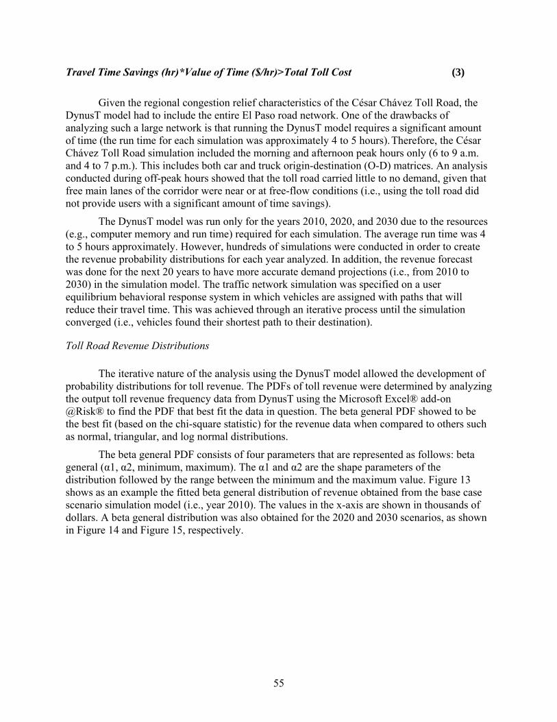
55

Travel Time Savings (hr)*Value of Time ($/hr)>Total Toll Cost (3)

Given the regional congestion relief characteristics of the César Chávez Toll Road, the DynusT model had to include the entire El Paso road network. One of the drawbacks of analyzing such a large network is that running the DynusT model requires a significant amount of time (the run time for each simulation was approximately 4 to 5 hours). Therefore, the César Chávez Toll Road simulation included the morning and afternoon peak hours only (6 to 9 a.m. and 4 to 7 p.m.). This includes both car and truck origin-destination (O-D) matrices. An analysis conducted during off-peak hours showed that the toll road carried little to no demand, given that free main lanes of the corridor were near or at free-flow conditions (i.e., using the toll road did not provide users with a significant amount of time savings).

The DynusT model was run only for the years 2010, 2020, and 2030 due to the resources (e.g., computer memory and run time) required for each simulation. The average run time was 4 to 5 hours approximately. However, hundreds of simulations were conducted in order to create the revenue probability distributions for each year analyzed. In addition, the revenue forecast was done for the next 20 years to have more accurate demand projections (i.e., from 2010 to 2030) in the simulation model. The traffic network simulation was specified on a user equilibrium behavioral response system in which vehicles are assigned with paths that will reduce their travel time. This was achieved through an iterative process until the simulation converged (i.e., vehicles found their shortest path to their destination).

Toll Road Revenue Distributions

The iterative nature of the analysis using the DynusT model allowed the development of probability distributions for toll revenue. The PDFs of toll revenue were determined by analyzing the output toll revenue frequency data from DynusT using the Microsoft Excel® add-on @Risk® to find the PDF that best fit the data in question. The beta general PDF showed to be the best fit (based on the chi-square statistic) for the revenue data when compared to others such as normal, triangular, and log normal distributions.

The beta general PDF consists of four parameters that are represented as follows: beta general (α1, α2, minimum, maximum). The α1 and α2 are the shape parameters of the distribution followed by the range between the minimum and the maximum value. Figure 13 shows as an example the fitted beta general distribution of revenue obtained from the base case scenario simulation model (i.e., year 2010). The values in the x-axis are shown in thousands of dollars. A beta general distribution was also obtained for the 2020 and 2030 scenarios, as shown in Figure 14 and Figure 15, respectively.

56

Figure 13: César Chávez Toll Road PDF of Revenue for the Base Case Scenario

Figure 14: César Chávez Toll Road PDF Revenue for the 2020 Scenario

0

0.5

1

1.5

2

2.5

3

1 2 3 4 5 6 7 8 9

Values x 10^

‐4

Values in Thousands

BetaGeneral(2.4457, 1.3815, 1970.4, 8586.5)

0

0.5

1

1.5

2

2.5

3

3.5

4

4.5

5

3 4 5 6 7 8 9 10

Values x 10^

‐4

Values in Thousands

BetaGeneral(3.392, 8.953, 3898.107, 10749.056)

57

Figure 15: César Chávez Toll Road PDF of Revenue for the 2030 Scenario

César Chávez Toll Road—Contingent Claims Analysis

A discounted cash flow financial model was developed to analyze the CRRMA’s risk exposure to toll revenue risk on the César Chávez Toll Road. A key hypothetical assumption in this analysis was that the CRRMA would be providing a traffic revenue guarantee (MGI) to a potential private concessionaire, equivalent to 75 percent of the expected toll revenue, as determined by an independent traffic and revenue forecast.19 The model was set up to evaluate traffic revenue risk using the methodological framework developed in Chapter 4.

Using the methodology developed in Chapter 4 and illustrated in Figure 10, the value of the revenue guarantee, or contingent liability assumed by the CRRMA, can be priced using Monte Carlo simulation on the toll road financial model and interpreting it as a put option. In this put option, the concessionaire has the right to “sell” the project’s value and receive the guaranteed amount (i.e., the annual MGI). When toll revenue performance matches or exceeds the MGI, the CRRMA’s contingent liability or guarantee has no value (Gu = 0). Conversely, when toll revenue underperforms and the guaranteed revenue fails to materialize, the guarantee trigger becomes operative with a positive guarantee value, as shown in Equation (1) (see Chapter 4). The value of the guarantee (G) will be equal to the PV of the total toll revenue shortfall (Gd) that the CRRMA guarantees over the life of the concession (20 years, from 2010 to 2030), as laid out in Equation (2).

Because of the uncertainties associated with toll road traffic volumes and revenue with respect to the VoT, the value of G is not predictable and follows a probability distribution. This

19 No analysis was conducted in this study to determine whether or not a guarantee was justified for the project. This study

assumes that a guarantee is justified by the project. The detailed traffic forecast can be found in Valdez-Ceniceros (48).

0

0.2

0.4

0.6

0.8

1

1.2

1.4

1.6

18 20 22 24 26 28 30 32

Values x 10^

‐4

Values in Thousands

BetaGeneral(4.3689, 16.525, 18754, 48420)

58

probability distribution was obtained by using the toll revenue model and Monte Carlo simulation on the toll revenue, using as a basis the PDFs for toll revenue in years 2010, 2020, and 2030, as illustrated in Figure 13, Figure 14, and Figure 15, respectively. The values for the PDF parameters of intermediate years had to be obtained through interpolation.

The annual revenue projections for the toll road were calculated using the expected value for the simulation variables, producing a static pro-forma cash flow. The MGI was assumed to be 75 percent of the pro-forma cash flows, that is, the expected annual toll revenue values. The simulated output from the financial model was used to determine the probability distribution for G, that is, the present value of the sum of the differences between the MGI static annual cash flow values and the values simulated. The resulting probability distribution is shown in Figure 16. In addition to the probability distribution of G, key statistics of G were calculated and are shown in Table 3.

Figure 16: Probability Distribution for Total Toll Revenue Shortfall (G)

Table 3: César Chávez Toll Road Guarantee—Statistics and Results G Statistics (at 10,000 Iterations) Value

Mean $259,294 Median $166,926 Standard Deviation $289,581 Skewness 1.31 Kurtosis 4.60 Coeff. of Variability 1.12 90th Percentile $ 670,421

0%

5%

10%

15%

20%

25%

30%

35%

$20 $230 $440 $660 $870

Prob

ability

Guarantee Values in US$ Thousands

59

As discussed in Chapter 4, a key issue is to determine which of the G statistics represents a fair value of the put option, or guarantee. Using the statistics most commonly recommended in the literature (i.e. the mean and the median), the results of this analysis indicate that the value of the CRRMA’s guarantee G to the concessionaire could be interpreted as having a value of US$259,294 (the mean) or US$166,926 (the median). Out of these two measures of risk exposure, the mean is clearly more conservative and likely the value that the guarantee underwriter (the CRRMA, in this case) would choose. On the other hand, if the 90th percentile were used (a far more conservative figure as opposed to the mean or the median), the value of the guarantee would then be $670,421.

Considering that according to the revenue analysis, the César Chávez Toll Road is expected to yield $81.9 million in PV of revenue at 90 percent confidence, the resulting $259,294 suggests it would not be too costly to provide the guarantee. However, in the context of VfM, this would mean that in a PSC analysis, the CRRMA would consider the guarantee cost as part of the retained risk (risk not transferred to the concessionaire), increasing the cost of the PPP option (reducing its VfM).

TRANSPORTATION REINVESTMENT ZONE PROJECT CASE STUDY

This section presents an analysis of public sector risk exposure in the City of El Paso TRZ No. 2 and 3, in El Paso, Texas. TRZs are a form of innovative financing recently created in the State of Texas that is based on the concept of VC. This section begins with a brief overview of VC as a non-commercial alternative form of PPP, and of the Texas TRZ concept. Next, this section describes of the City of El Paso TRZ No. 2 and 3, its geographic limits, and the institutional and financial arrangements for its implementation.20 Finally, the section closes with the CCA analysis of the City of El Paso TRZ revenue risk exposure.

Value Capture as a PPP—The Texas TRZ Model and Revenue Risk Characteristics

VC is an innovative financing method that relies on leveraging the real estate potential brought by urban asset improvements. VC can be defined as the means by which capital infrastructure investment is financed through means of “capturing” either some or all of the added value of real estate property that results directly from that investment (1). Vadali and Aldrete note that VC is a way of using and recycling transportation project public benefit revenue streams to fund specific projects within those zones. These revenue streams provide the opportunity to adopt project bond financing in designated zones. As such, it is a non-commercial form of PPP, a feature that distinguishes it from other forms of PPP (1).

Legislation adopted by the State of Texas in 2007 makes specific provisions for the development of municipal TRZs, a concept that encapsulates the principles of VC to supplement roadway project financing.21 TRZs are a mechanism for local governments to leverage local and

20 The reader is referred to Vadali et al. for a more detailed discussion on VC and TRZ revenue potential estimation in the El

Paso region (44). 21 Texas SB 1266 can be found at http://www.legis.state.tx.us/tlodocs/80R/billtext/pdf/SB01266F.pdf#navpanes=0.

60

state funds for infrastructure construction by using TxDOT’s “pass-through” mechanism.22 After designating a contiguous area along a corridor as a TRZ, a local government entity (a city or a county) can securitize the incremental tax revenues along with TxDOT pass-through financing to obtain the funds necessary to bring a project to fruition. Funds generated from the securitization will be used to pay for transportation infrastructure projects in the TRZ, and investors will be repaid from the combined revenue stream—the incremental tax revenues and TxDOT pass-through funds. Once the securitized debt is repaid, the additional revenues generated by the TRZ go back to the municipality’s general fund and are redirected toward other municipal services (1). However, with property tax revenue dependent on real estate prices and the pace of development in the region, there is a significant amount of uncertainty and risk associated with debt repayment. The flow of funds and risk allocation associated with TRZ finance is described in Box 10 and illustrated in Figure 17.

Box 10: Flow of Funds and Revenue Risk in Texas TRZ Financing (43) The flow of funds as conceptualized in the SB 1266 TRZ model is shown in Figure 17. As shown in the figure, every year during the life of the TRZ, tax revenue collected over and above an agreed-upon base would go into an ad valorem tax increment account established by the local government. From the ad valorem tax account, these funds would flow to the designated local entity (the local government itself or a Regional Mobility Authority), where they would be complemented with pass-through funds. Finally, the designated local entity would securitize this annual revenue stream to obtain debt and fund construction of the transportation facilities. In terms of revenue risk, the TRZ legislation is neither clear nor explicit regarding its allocation, while the flow of funds shown in the figure seems to implicitly allocate the risk of financial non-performance to the designated local entity issuing debt.

In practice, the annual cash flow projections from the TRZ are estimated prior to its establishment and represent simply a projection and not a binding commitment for the municipality. Rather, the municipality commits the entire tax increment in any given year over the TRZ life, regardless of whether the amount falls short or exceeds the projection. Consequently, the TRZ revenue securitized represents a contingent liability for the designated local entity, whose commitment to repay debt according to a pre-specified schedule remains. The risk to bondholders in such a situation can be defined as the risk that property values within the TRZ do not perform as expected or development does not occur as planned. In such a case, the designated local entity would face a shortfall in revenue, while keeping the obligation to meet its debt service according to schedule.

22 TxDOT defines pass-through financing as a mechanism for project developers to finance and be reimbursed for the capital

costs of constructing or expanding a state highway project. The public agency (e.g., a local government) or private entity developing the project finances, builds, maintains, and/or operates a road project, and TxDOT reimburses a portion of the project cost by making periodic payments for each vehicle that drives on the highway. The remainder of the project capital costs may be met via a combination of traditional construction funds, toll revenue, or TRZ revenue (46).

61

Figure 17: Conceptual Flow of Funds for TRZ Financing

The City of El Paso TRZ No. 2 and 3

One of the first examples of the application of the TRZ model is in El Paso, Texas. The City of El Paso established its Transportation Reinvestment Zones No. 2 and 3 in May 2010. El Paso’s RMA, the CRRMA, has entered into an agreement with TxDOT and the City of El Paso to finance a series of transportation improvement projects within the City of El Paso’s TRZ No. 2 and 3 using a mix of TRZ and pass-through funds. The CRRMA will be the entity responsible for securitizing debt backed by property tax revenues from the City of El Paso TRZs and TxDOT pass-through funds.

The total present value of the TRZ funding commitment of the City of El Paso to the CRRMA is approximately US$70 million, which is to be repaid from the proceeds of the property tax increment collected by the city each year for approximately 30 years. Given their dependence on the real estate market, these cash flows are by nature bound to be significantly uncertain. On the other hand, the City of El Paso has committed to deliver a certain cash flow stream to the CRRMA. The City of El Paso is therefore exposed to the risk that the property tax increment revenue expected does not materialize, while its obligation to the CRRMA remains firm, creating a contingent liability for the city.

Geographic Limits of the City of El Paso TRZ No. 2 and 3

Research has documented that the improvement or addition of transportation capacity along a corridor has a positive effect on real estate values within buffer zones of up to 2 miles in radius from the corridor’s centerline (44). The boundaries of the TRZ No. 2 and 3 were defined by estimating the minimum buffer from the centerline of the corridors within the 2-mile

Pass‐through Payments

TxDOT

Public Entity(City, County, RMA)

or Agent

• Pass‐throughAgreement

• Issue Bonds

Ad Valorem Tax Increment Account

City and/or County

Transportation Reinvestment Zone

Design & construction costs

Facility manager/ operator

Engineer/ construction contractor

Maintenance & operation costs

Financial institutions/ markets

Debt Repayments

Surplus upon TRZ termination may be used for other transportation projects within or outside TRZ

100% Tax increment payments

62

maximum that would allow collecting the tax increment revenue equivalent to a PV of US$70 million over the 30-year period (45).

The sizes of the buffers developed along the corridors ranged from 1/16 of a mile to 1/2 mile from the centerline, varying from corridor to corridor and within the same corridor. The resulting combined acreage of the 2,481 parcels in both TRZs is 9,947 acres, for a total 2010 taxable value of about US$1.2 billion. These parcels generated annual property tax revenues for the City of El Paso of almost US$7.6 million in 2010. About 78 percent of this acreage (7,791 acres) is currently undeveloped land, and therefore this land holds the most potential for VC over the 30-year analysis period.

The TRZ No. 2 consists of the five corridors listed below and includes a buffer zone of varying widths around each of them, as shown in Figure 18(a):

• Corridor 2.1. I-10, from Transmountain Rd to Sunland Park Dr. • Corridor 2.2. Sunland Park Dr, from I-10 to N Mesa St. • Corridor 2.3. N Mesa St, from Sunland Park Dr to Glory Rd; Glory Rd, from

N Mesa St to N Oregon St; and N Oregon St, from Glory Rd to Montana Ave. • Corridor 2.4. Montana Ave, from N Oregon St to Joe Battle Blvd. • Corridor 2.5. Loop-375, from N Loop Dr (Alameda Ave) to Montana Ave;

N Zaragoza Rd, from Tierra Este Rd to Joe Battle Blvd; and I-10, from Zaragoza Rd to the city limits.

The TRZ No. 3 consists of the three corridors listed below and includes a buffer zone of varying widths around each of them. Figure 18(b) illustrates its geographic limits.

• Corridor 3.1. NE Parkway (proposed), from the city limits of Fort Bliss to the New Mexico state line.

• Corridor 3.2. Transmountain Rd, from Railroad Dr to US-54 (Patriot Freeway). • Corridor 3.3. Dyer St, from Transmountain Rd to the NE Parkway corridor.

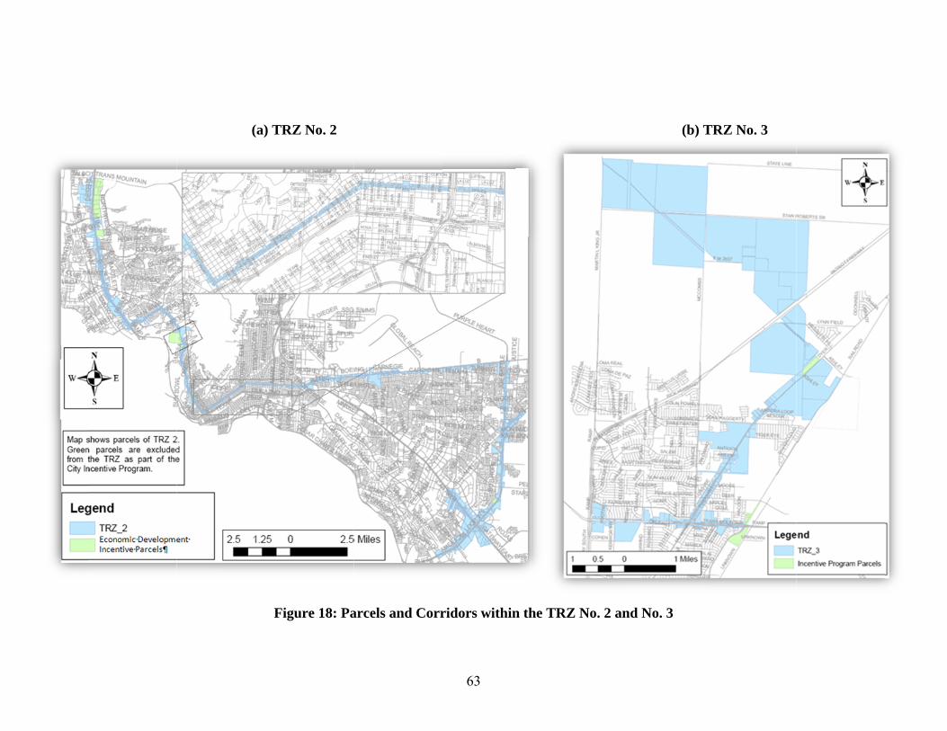
(a)) TRZ No. 2

Figure 18: Paarcels and Corr

63

ridors within th

he TRZ No. 2 a

(b) T

and No. 3

TRZ No. 3

64

Revenue Analysis of the City of El Paso TRZ No. 2 and 3

The authors assisted the City of El Paso in conducting the analysis of TRZ revenue potential and in the implementation of TRZ No. 2 and 3 (45). The analysis framework used was based on key drivers of property value growth when a capacity improvement project is implemented along a transportation corridor, as described in Box 11. Property values are sensitive to capacity improvements and macroeconomic conditions; properties located near an infrastructure project capitalize economic benefits over time. Only projects that generate large accessibility changes, cultivate economic development, and lead to regional mobility improvements foster the potential to generate TRZ revenues. Under this framework, smaller scale projects, like aesthetic improvements, are not considered significant revenue generators.

Box 11: TRZ Revenue Potential Assessment The assessment of TRZ revenue potential along each corridor required conducting the following analyses:

• Identify the geographic extent of which capacity improvements produce economic impacts on property values and development trends to determine the TRZ boundary.

• Quantify the real estate inventory within the TRZ and the associated taxable property values. • Identify the type of land uses for vacant and non-vacant parcels—commercial, industrial, residential,

agricultural, etc.—and their development trends. • Estimate the pace or speed of vacant land development—the pace of absorption. • Approximate the timing of development from the opening date of an infrastructure project. • Calculate the property values attained upon development for both existing property uses and newly

developed land.

To conduct the analysis of revenue potential and define the TRZ boundaries, a discounted cash flow model linking a geographic information systems (GIS) database with parcel information to key input parameters was developed.23 Outputs from the revenue analysis include the annual cash flows for TRZ tax increment revenue over a 30-year analysis period, along with an analysis of the PV of these cash flows, and the expected bonding capacity.

City of El Paso TRZ No. 2 and 3—Contingent Claims Analysis

Using the City of El Paso TRZ No. 2 and 3 developed by the researchers to evaluate its revenue potential, an analysis of the City of El Paso’s revenue risk exposure was conducted. The analysis assumes that the City of El Paso is providing a revenue guarantee to the CRRMA. The model was set up to evaluate revenue risk stemming exclusively from land-market responses for TRZ finance only (specifically excluding the pass-through component), using the CCA-approach methodological framework developed in Chapter 4.

Using the methodology developed in Chapter 4 and illustrated in Figure 10, the value of the TRZ revenue guarantee, or contingent liability assumed by the City of El Paso, can be priced using Monte Carlo simulation on the financial cash flow model of the TRZ and interpreting it as a put option. In such a hypothetical put option, the CRRMA has the right to “sell” the project’s value and receive the guaranteed amount (i.e., the TRZ annual cash flow). When TRZ performance matches or exceeds projections, the city’s contingent liability or guarantee has no 23 For a complete description of the analysis, the reader is referred to Bujanda et al. (45).

65

value (Gu = 0). Conversely, when the TRZ underperforms and projected revenues fail to materialize, the guarantee trigger becomes operative with a positive guarantee value, as shown in Equation (1) in Chapter 4. The value of the guarantee (G) will be equal to the PV of the total TRZ revenue shortfall (Gd) that the City of El Paso guarantees over the life of the TRZ (30 years, from 2010 to 2040), as laid out in Equation (2).

Because of the uncertainties in property values and pace of development, the value of G is not predictable and follows a probability distribution. This probability distribution was obtained by using the TRZ financial model and Monte Carlo simulation on the following three key variables: a) vacant land developed (for commercial, industrial, and residential zoning); b) pace of vacant land development (for commercial, industrial, and residential zoning); and c) property value growth rates for parcels located around transportation improvements (for commercial, industrial, and residential zoning). The PDFs for each of the variables are described in detail in Vadali et al. (44).

The annual revenue projections to be produced by the TRZ are calculated using the expected value for the simulation variables, producing a static pro-forma cash flow. The pro-forma cash flow resulting from the expected variable values is considered the MGI guaranteed by the city to the CRRMA. The simulated output from the financial model was used to determine the probability distribution for G, that is, the present value of the sum of the differences between the static annual cash flow values and the values simulated. The resulting probability distribution is shown in Figure 19 and Figure 20. In addition to the probability distribution of G, key statistics of G were calculated and are shown in Table 4.

Figure 19: Probability Distribution for Total TRZ No. 2 Guarantee (G)

0%

5%

10%

15%

20%

25%

30%

35%

40%

$50 $1,030 $2,010 $2,990 $3,980

Prob

ability


66

Figure 20: Probability Distribution for Total TRZ No. 3 Guarantee (G)

Table 4: TRZ No. 2 and 3 Guarantee—Statistics and Results G Statistics (at 10,000 Iterations) TRZ No. 2

Value TRZ No. 3

Value Mean $1,128,418 $220,697 Median $547,188 $111,550 Standard Deviation $1,375,660 $259,354 Skewness 1.36 1.26 Kurtosis 4.34 3.92 Coeff. of Variability 1.22 1.18 90th Percentile $3,232,047 $620,050

As discussed in Chapter 4, a key issue is to determine which of the G statistics represents a fair value of the put option, or guarantee. Using the statistics most commonly recommended in the literature (i.e. the mean and the median), the results of the CCA indicate that the value of the City of El Paso’s guarantee (G) to the CRRMA could be interpreted as follows:

• TRZ No. 2: o Mean value – G = US$1,128,418 o Median value – G = US$547,188

• TRZ No. 3: o Mean value – G = US$220,697 o Median value – G = US$111,550

In the case of the TRZ No. 2 and 3, the mean value is obviously more conservative and would very likely be the preferred option of the party underwriting the guarantee (the City of El Paso). Based on this analysis, the value of the City of El Paso’s cost of risk exposure to TRZ revenue would be about US$1,349,115.

0%

5%

10%

15%

20%

25%

30%

35%

$10 $210 $400 $590 $780

Prob

ability


67

CHAPTER 6: CONCLUSIONS AND RECOMMENDATIONS

This report reviewed the U.S. and international experience with dealing with public sector risk exposure in transportation infrastructure PPP agreements in the context of VfM, a central tenet to the pursuit of PPPs. This analysis concluded with a set of lessons learned relevant to the development of transportation infrastructure through PPPs in the U.S. Among the key lessons learned was the importance of having a framework in place to evaluate and quantify public sector risk exposure to enable the integration of the cost of risk bearing into the analysis of VfM in PPP agreements.

Next, the report examined some of the methods and practices that have already been tried and tested internationally to value risk exposure in infrastructure PPPs. Based on these methods and practices, a methodological framework to value contingent liabilities as a proxy for public sector risk exposure was developed. To facilitate the understanding of the framework and its application to actual projects, a step-by-step methodology was also developed.

Finally, the report presented the application of the methodology to two different U.S. transportation PPP case studies in Texas. The first case study was a standard concession-type toll road where the analysis focused on the public sector risk exposure resulting from a hypothetical minimum revenue guarantee to a private concessionaire. The second case study was a non-standard, non-commercial form of PPP particular to the state of Texas that relies on the principle of value capture, where the analysis focuses on the public sector risk exposure resulting from property tax revenue volatility.

The first section of this chapter presents the main conclusions of this study. The second and last section presents recommendations for future research. Both the conclusions and recommendations complement the findings of the 2008 GAO report to the U.S. Congress, “Highway Public-Private Partnerships: More Rigorous Up-front Analysis Could Better Secure Potential Benefits and Protect the Public Interest,” discussed in this report (15).

CONCLUSIONS

The main conclusions of this research are the following:

1. The cost of public sector risk bearing is an important element to consider when evaluating PPP proposals and should be introduced in the evaluation of U.S. PPPs.

• Most countries with advanced PPP programs include the valuation of public sector risk as a key step in their analysis of PPP proposals. The evidence for this ranges from developing countries where providing specific risk guarantees to the private sector is sometimes necessary to attract private investment, to developed countries, such as Australia, where the cost of bearing risk is a key driver of the VfM and PSC analyses performed when deciding whether a project should be implemented as a PPP or a traditional procurement.

• The review of transportation PPP projects in several U.S. states revealed that a systematic, methodological approach to quantify in monetary terms public sector risk exposure in the analysis of PPP projects does not exist. There have been some

68

isolated attempts at conducting analyses similar to the Australian PSC (e.g., Texas SH 121), but these analyses have not included the cost of risk bearing, fundamental to the VfM concept that drives PSC analyses, as a consideration when deciding to pursue a project as a PPP.

• Although the U.S. transportation PPP projects reviewed had a clear delineation of the risks that would be retained by the government, none of them appeared to have determined the preferred risk allocation using an approach based on a monetary measure of the cost of risk bearing and VfM.

2. The methodologies that have been tried and tested internationally to value public sector risk exposure can be effectively adapted and applied to the analysis of U.S. transportation PPP projects.

• Contingent liability valuation methods such as actuarial, statistical, and econometric methods have been widely used in the U.S. and internationally to measure public sector risk exposure in the financial sector (e.g., savings deposit insurance, mortgage insurance). However, their applicability to transportation infrastructure projects is not practical given their unique nature.

• Contingent claim methods, such as the CCA approach, have been successfully used internationally to quantify in monetary terms public sector risk exposure in infrastructure PPP projects, including those in the transportation sector.

• A methodological framework based on the CCA approach was developed and successfully applied to two very different U.S. transportation PPP projects, demonstrating that the methodologies that have been successfully tried and tested internationally have potential to be adapted and used in U.S. PPP projects.

RECOMMENDATIONS

There are three main recommendations that stem from this research. These include both policy recommendations for transportation agencies, as well as recommendations for future research.

1. Incorporate the concept of VfM in the analysis of U.S. transportation PPP projects.

• This research demonstrated that formally adopting the use of the concept of VfM in the U.S. would be very beneficial given the expanding role that PPPs are playing in financing the development of the U.S. transportation infrastructure network. This study also demonstrated that U.S. practice can benefit significantly from the practices that have been tried and tested internationally.

• In terms of future research, this study was limited to developing and applying a methodology to value public sector risk exposure. However, this study could be complemented or expanded by adapting a method that incorporates the concept of VfM, such as the PSC. This new research would involve adapting a method such as the PSC for use in U.S. case studies and, using the methodology developed in this research, estimating the risk-adjusted cost and benefits of a proposed PPP project by comparing two alternative hypothetical scenarios, one assuming a private sector delivery and one assuming a public sector delivery.

69

2. Define eligibility criteria or decision rules to determine acceptable risk exposure.

• U.S. transportation agencies can benefit from defining what risks they will retain in a PPP using an approach based on an objective measure of the cost of risk bearing. This approach would ensure that the preferred risk allocation is the one that maximizes VfM.

• Future research could be focused on analyzing case studies of U.S. PPP projects to assess the monetary cost of risk bearing associated with the selected risk allocation and could try to identify standard criteria decision rules that transportation agencies could develop and adapt for future projects. An example would be the cost of non-compete clauses that prevent the construction of new capacity within a certain radius of a toll road concession project. In such a case, criteria for different radii sizes could be developed to optimize the cost of risk bearing.

3. Research the need for and viability of implementing risk management mechanisms that support pooling and diversifying public sector PPP risk exposure in U.S. states.

• The risk mitigation concepts discussed in this report described how diversifying a project portfolio can limit losses in the event of the materialization of a risk in a particular project through the distribution of its investments among different projects.

• The review of international experience showed that some countries have in place contingent liability management mechanisms at the national level to pool and diversify PPP infrastructure project risks. These often take the form of guarantee funds that back the financial obligations of implementing agencies, lowering their cost of borrowing and facilitating the transaction. Some of these guarantee programs rely on fees charged to beneficiaries to cover the cost of the guarantees provided, similar to the way insurance companies charge premiums to customers.

• As states in the U.S. move toward increased use of PPPs to close the infrastructure gap, the need for and adequacy of establishing similar programs at the state and federal levels should be evaluated. Such guarantee programs would pool various types of contingent liabilities acquired by implementing agencies (e.g., state and local transportation agencies) in diverse PPP projects located throughout a particular state.

71

REFERENCES

1. Vadali, Sharada and Aldrete, Rafael M. Transportation Finance, Public Private Partnerships, and Contingent Liabilities: Case Evidence from a Value Capture Venture from Texas. Paper Presented at the 89th Transportation Research Board Annual Meeting. Washington, DC : Transportation Research Board, January 2010. 2. Castalia Strategic Advisors. Guidelines for Structuring Public-Private Partnerships. Washington, DC : Castalia Strategic Advisors, 2009. 3. Aldrete, Rafael M. Feasibility Evaluation Model for Toll Highways. Doctoral Dissertation. Austin : The University of Texas at Austin, 1998. 4. The World Bank. Tool for Public-Private Partnerships for Roads and Highways. [Online] Public Private Infrastructure Advisory Facillity. [Cited: 10 01, 2010.] http://www.ppiaf.org/ppiaf/sites/ppiaf.org/files/documents/toolkits/highwaystoolkit/1/1-13.html. 5. HM Treasury. The UK's Economics & Finance Ministry. Value for Money Assessment Guidance. [Online] November 2006. http://www.hm-treasury.gov.uk/d/vfm_assessmentguidance061006opt.pdf. 6. OCDE. Public-Private Partnerships: In Pursuit of Risk Sharing and Value for Money. Paris : Organization for Economic Co-operation and Development, 2008. 7. Department of Treasury and Finance. Public Sector Comparator Technical Note. Partnerships Victoria. [Online] [Cited: April 20, 2009.] http://www.partnerships.vic.gov.au/CA25708500035EB6/WebObj/TechnicalNote-PSCTechnicalNote1-Entire/$File/Technical%20Note%20-%20PSC%20Technical%20Note1%20-%20Entire.pdf. 8. Irwin, Timothy. Government Guarantees: Allocating and Valuing Risk in Privately Financed Infrastructure Projects. Washington, DC : The World Bank, 2007. 9. Irwin, Timothy, et al. Managing Government Exposure to Private Infrastructure Risks. The World Bank Research Observer. 1999, Vol. 14, 2. 10. Irwin, Timothy. Public Money for Private Infrastructure: Deciding When to Offer Guarantees, Output-Based Subsidies and Other Fiscal Support. Washington, DC : The World Bank, 2003. World Bank Working Paper. No. 10. 11. Blommenstein, Hans J. How to Integrate Contingent Liabilities in Public debt Management Strategies? Paris : International Monetary Fund High-level conference on Fiscal Risks, 2008. 12. Secretariat for the Committee on Infrastructure. Financing Infrastructure Projects through the India Infrastructure Finance Company Limited (IIFCL). New Delhi : Planning Commission, Government of India, 2009. 13. Shin, Sunghwan. Approaches for PPP Risk Sharing and Risk Management in Korea. Knowledge Sharing on Infrastructure Public-Private Partnerships in Asia. Seoul : Asian Development Bank, 2009. 14. Cheah, Charles Y.J. and Liu, Jicai. Valuing Governmental Support in Infrastructure Projects as Real Options Using Monte Carlo Simulation. s.l. : Journal of Construction Management and Economics, 2006. 24. 15. Government Accountability Office. Highway Public-Private Partnerships: More Rigorous Up-front Analysis Could Better Secure Potential Benefits and Protect the Public Interest. Washington, DC : United States Government Accountability Office, 2008. GAO-08-44. 16. Dallas Citizens Council. DCC plays instrumental role in NTTA/SH 121 win. Dallas Citizens Council Report. Dallas, TX : Dallas Citizens Council, 2007. Fall.

72

17. North Texas Tollway Authority. Toll Road History - State Highway (SH) 121. Collin, Dallas and Denton Counties. 2007. 18. —. Executive Summary State Highway 121 Proposal. State Highway 121 Proposal. Dallas, TX : North Texas Tollway Authority, 2007. 19. Speeds on New Texas 130 South TR major $-issue. Toll Road News. [Online] July 6, 2006. [Cited: July 6, 2010.] http://www.tollroadsnews.com/node/3433. 20. Russell, Phillip E. Comprehensive Development Agreements: SH 130 (Segments 5&6) - Testimony Before the Legislative Study Committee on Private Participation in Toll Projects. The Texas Senate. [Online] July 22, 2008. [Cited: September 9, 2009.] 21. —. Public-Private Partnerships: Texas Style. American Association of State Highway and Transportation Officials. [Online] July 23, 2008. [Cited: September 9, 2009.] http://audit.transportation.org/Documents/Wed2-PhilRussell.pdf. 22. Indiana Toll Road. About ITR. Indiana Toll Road. [Online] [Cited: January 23, 2009.] https://www.getizoom.com/aboutITR. 23. The Times of Northwest Indiana. State to pay for Indiana Toll Road Free Time. The Times of Northwest Indiana. [Online] September 20, 2008. [Cited: January 20, 2009.] http://www.nwi.com. 24. Cintra. Cintra Annual Report. Cintra. [Online] 2008. [Cited: January 15, 2009.] http://www.cintra.es/recursos/doc/Accionistas_e_Inversores/Informe_Anual/12971_2742742009155340.pdf. 25. Chicago Skyway. About the Skyway. Chicago Skyway. [Online] 2005. [Cited: January 23, 2009.] http://chicagoskyway.org/. 26. Johnson, Craig L., Luby, Martin J. and Kurbanov, Shokhrukh I. Toll Road Privatization Transactions: The Chicago Skyway and Indiana Toll Road. Washington, D.C. : Association for Budgeting and Financial Management, 2007. 27. Morallos, Dorothy, et al. Value for Money Analysis in U.S. Transportation Public–Private Partnerships. Washington DC : Transportation Research Board of the National Academies, 2009. Vol. 2115. 0361-1981. 28. Irwin, Timothy, et al. Dealing with Public Risk in Private Infrastructure. Washington, DC : The World Bank, 1997. ISBN 0-8213-4030. 29. Irwin, Timothy and Mokdad, Tanya. Managing contingent liabilities in public-private partnerships: Practice in Australia, Chile, and South Africa. Washington, DC : The World Bank, 2009. 30. Republic of South Africa National Treasury PPP Unit. South African Public Private Partnerships. PPP Manual. [Online] [Cited: 10 5, 2010.] http://www.ppp.gov.za/. 31. Public-Private Partnerships, Government Guarantees, and Fiscal Risk. International Monetary Fund. Washington, DC : International Monetary Fund, 2006. 32. Victoria, State Government of. Partnerships Victoria. [Online] 2010. http://www.partnerships.vic.gov.au. 33. New South Wales Treasury. NSW Treasury submission to Infrastructure Australia - National public private partnerships guidelines - NSW jurisdictional requirements. Working With Government. [Online] 2009. [Cited: October 3, 2010.] http://www.wwg.nsw.gov.au/__data/assets/pdf_file/0018/13509/National_PPP_guidelines_nsw_jurisdictional_requirements.pdf.

73

34. Aldrete-Sanchez, Rafael M., Tucker, Richard L. and McCullough, Ben F. Feasibility Evaluation Model for Toll Highways. College Station, TX : Southwest Region University Transportation Center - Texas Transportation Institute, 2005. Report 467502-2. 35. International Accounting Standards Board. International Financial Reporting Standards (IFRSs)—Including International Accounting Standards (IASs) and Interpretations as at 31 March 2004. London : International Accounting Standards Board, 2004. p. 2169. 36. Almeyda, Miguel and Hinojosa, Sergio. Revision of the State of the Art Contingent Liability Management. Washington, DC : The World Bank, 2001. 37. Lewis, Christopher and Mody, Ashoka. The Management of Contingent Liabilities: A Risk Management Framework for National Governments. Ashoka Mody’s Web Site of Publications. [Online] 1998. [Cited: August 1, 2009.] http://www.amody.com/pdf/lewis.pdf. 38. Mody, Ashoka and Patro, Dilip. Methods of Loan Guarantee Valuation and Accounting. s.l. : CFS Discussion Paper Series, 1995. 116. 39. Brandao, Luiz E.T. and Saraiva, Eduardo C. G. Valuing Government Guarantees in Toll Road Projects. Berkeley, CA : Annual International Conference on Real Options: Theory Meets Practice - Real Options Group, 2007. 40. Razgaitis, Richard. Dealmaking Using Real Options and Monte Carlo Analysis. Hoboken, N.J. : John Wiley & Sons, 2003. 41. State of Texas. Section 228.0111: Toll Projects of Local Toll Project Entities. Texas Transportation Code. Austin : s.n., 2009. 42. Bain, Robert and Polakovic, Lidia. Traffic Forecasting Risk Study Update. s.l. : Standard & Poor's, 2005. 43. Vadali, Sharada, et al. Planning Tools to Assess the Real Estate Leveraging Potential for Roadways and Transit. Austin, TX : Texas Department of Transportation, 2010. 0-6538. 44. Vadali, Sharada, Aldrete, Rafael M. and Bujanda, Arturo. A Financial Model to Estimate the Value Capture Potential for Roadways. Washington, DC : Transportation Research Record, 2009. 45. Bujanda, Arturo, et al. Assessment of Recalibration Needs for the City of El Paso TRZ Boundaries. El Paso : Texas Transportation Institute, 2010. 46. Texas Department of Transportation. Pass-Through Financing. TxDOT: Open for Business. Austin : Texas Department of Transportation, 2007. 47. Queiroz, Cesar and Kirali, Henry. A Review of Institutional Arrangements for Road Asset Management: Lessons for the Developing World. Washington, DC : The World Bank, 2010. 48. Valdez-Ceniceros, Gabriel A. A Risk Analysis Framework for Toll Road Revenue Forecasts. Master's Thesis. El Paso, TX : The University of Texas at El Paso, 2010.

University Transportation Center for Mobility™


The Texas A&M University System

College Station, TX 77843-3135

Tel: 979.845.2538 Fax: 979.845.9761

utcm.tamu.edu

TexasTransportationInstitute