valuing employee stock options under sfas 123r using the black–scholes–merton and lattice model...

Journal of

J. of Acc. Ed. 25 (2007) 88–101

www.elsevier.com/locate/jaccedu

AccountingEducation

Teaching and educational note

Valuing employee stock options under SFAS123R using the Black–Scholes–Merton and

lattice model approaches

Charles Baril a,*, Luis Betancourt b, John Briggs c

a Frank & Company Faculty Fellow, MSC 0203, School of Accounting, James Madison University,

Harrisonburg, VA 22807, United Statesb Office of the Chief Accountant, Office of the Comptroller of the Currency 250 E Street,

SW Washington, DC 20219, United Statesc School of Accounting, James Madison University, Harrisonburg, VA, United States

Abstract

In 2004, the Financial Accounting Standards Board (FASB) issued Statement of Financial

Accounting Standard No. 123 (revised 2004), Share-Based Payments (SFAS 123R), requiring all enti-ties to recognize as expense the fair value of stock options issued to employees for services provided.Because employee stock options cannot be traded publicly, their fair value must be estimated using amodel, with the Black–Scholes–Merton (BSM) and lattice models being the most appropriatealternatives.

This teaching note provides an overview of employee stock options, followed by a discussion ofthe BSM and lattice valuation models, including their application and limitations. A project whichhas been used in financial accounting courses is also presented. The conceptual discussion coupledwith illustrated examples will help students enhance their understanding of fair value estimationof and accounting for employee stock options under the recently adopted SFAS 123R.� 2007 Elsevier Ltd. All rights reserved.

Keywords: Option pricing; Employee stock options; FASB 123; Lattice models

0748-5751/$ - see front matter � 2007 Elsevier Ltd. All rights reserved.

doi:10.1016/j.jaccedu.2007.01.002

* Corresponding author. Tel.: +1 540 568 3092.E-mail addresses: [email protected] (C. Baril), [email protected] (L. Betancourt), briggsjw@

jmu.edu (J. Briggs).

mailto:[email protected]

mailto:[email protected]

mailto:briggsjw@

C. Baril et al. / J. of Acc. Ed. 25 (2007) 88–101 89

1. Introduction

Companies grant options to align the incentives of employees with the incentives ofstockholders. Employee stock options are call options that give the holder the right, butnot the obligation, to buy a share of their company’s stock for a fixed price, called theexercise or strike price, during a specified period of time. Both employees holding stockoptions and stockholders benefit when the stock price rises. In addition to aligning incen-tives, stock options enable companies to compensate employees without paying out cash,an advantage of particular importance to start up companies. Further, certain companiesderive tax benefits from compensating employees with stock options rather than with cash.

Typical employee stock options have several features that distinguish them fromoptions that are publicly traded. First, employee stock options cannot be sold or trans-ferred by the employee. Second, employee stock options have a long period, typically10 years, over which they can be exercised, as opposed to the shorter terms of publiclytraded options. Third, most employee stock options have vesting restrictions requiringan employee to wait a specified period of time before exercising any options. This delayencourages the employee to continue serving the company rather than forfeit the options.

When stock options are awarded, the accounting objective is to recognize their value ascompensation expense over the period the company benefits from the employee’s service.However, because employee stock options cannot be traded publicly, one cannot simplylook to the market for a price to use as fair value. Two alternatives for valuing employeestock options were accepted prior to the issuance of SFAS 123R. The intrinsic value methodbased compensation expense on the intrinsic value of the option on the grant date, theamount by which the stock’s price exceeded the option’s exercise price. Since most employeeoptions are granted ‘‘at the money’’, the resulting compensation expense was zero.

In contrast, the fair value method based compensation expense on the fair value of theoption on the date granted. An option’s fair value exceeds its intrinsic value because fairvalue incorporates the value created by the probability that the stock’s price will rise abovethe option’s exercise price at some point during the option’s term. With higher value comeshigher compensation expense. Not surprisingly, most companies elected to measure com-pensation expense using the intrinsic value method, though they were required to disclosein their footnotes the fair value of the employee stock options granted.

In December 2004, the Financial Accounting Standards Board (FASB) issued State-

ment of Financial Accounting Standard No. 123 (revised 2004) Share Based Payments

(SFAS 123R), requiring all entities to recognize as expense the fair value of equity instru-ments issued to employees for services provided. Companies can no longer measure com-pensation expense using the option’s intrinsic value. A discussion and illustrated examplesof the BSM and lattice valuation models, two alternatives specified by SFAS 123R, follow.In addition, a project which has been used in financial accounting courses is presented.The conceptual discussion and the project will help students better understand the estima-tion of fair value of employee stock options under the recently adopted SFAS 123R.

2. Description of the models

The fair value of employee stock options must be estimated because the options are nottransferable; they cannot be traded publicly. SFAS 123R allows entities to value optionsusing either the BSM or lattice model, as long as the model selected is based on established

90 C. Baril et al. / J. of Acc. Ed. 25 (2007) 88–101

principles of financial economic theory and reflects all substantive characteristics of theoption.

2.1. Black–Scholes–Merton model

The more widely used BSM model was designed to value publicly traded options withshort exercise periods. The basic model assumes that the stock does not pay dividends andthat the option can be exercised only at the expiration date. Later variations relaxed theseassumptions. The value of a call option, C, is defined as a function of five variables underthe basic BSM model:

� S is the current price of the stock.� X is the exercise price of the option.� T is the expected life of the option (in years).� r is the volatility, the annualized standard deviation of the stock’s return.� r is the risk-free interest rate.

The BSM model formula is:

(1) C = SN(d1) � Xe�rtN(d2)

where
(2) N(d1) and N(d2) refer to probabilities under the standard normal distribution,(3) e equals 2.71828, the base of the natural logarithm,
(4) d1 ¼ lnðS=X Þþðrþ½r2=2�ÞTrffiffiffi

Tp and

(5) d2 ¼ d1� rffiffiffiffi

Tp

.

While the BSM model is complex and the formulas somewhat difficult to comprehend,the model is relatively simple to implement. Fig. 3 in Section 3.2 provides guidance forusing Excel to measure an option’s value with the BSM model.

Despite the BSM model’s complexity, an understanding of the foundation ideas is easilygrasped. Consider an option with the following data:

S = $100, X = $100T = 4 yearsr = 40%, r = 5%.

In this example, the option’s intrinsic value is zero at the grant date because the stockprice is equal to the option’s exercise price. If the stock price remains constant over theoption’s life, the option’s intrinsic value remains zero. However, it is probable that thestock price will surpass the exercise price over the four-year life of the option. An option’sfair value incorporates this potential. With a risk-free rate of 5%, the stock price isexpected to increase by 5% per year compounded continuously. Under the simplified sce-nario of 0% volatility, the stock price will rise to $122.04 after four years. The benefit tothe option holder will then be $22.04, the option’s intrinsic value. To measure the option’svalue at the grant date, the $22.04 intrinsic value at the exercise date is discounted at the5% risk-free rate for four periods, generating a fair value of $18.13.


An option’s value increases with increases in both the life of the option, T, and the risk-free rate, r. The faster the stock price is expected to grow and the longer the stock price cangrow, the higher the expected stock price at the option’s exercise date.

Much of the complexity of the BSM model relates to volatility, the degree of unpredict-able change in the stock price over time. While this stock price change can be eitherincreasing or decreasing, volatility adds value to the option. Potential increases in stockprice increase the option’s intrinsic value and fair value. Conversely, potential decreasesdo not diminish value. If the stock price falls below the option’s exercise price, the optionholder will choose to let the option expire. Consequently, when 40% volatility is incorpo-rated in the example, the option’s fair value rises to $38.16.1

While relatively easy to implement and understand at a fundamental level, the BSMmodel is difficult to modify and requires satisfying specific assumptions. Option valuationusing the more adaptable lattice model is presented next.

2.2. Lattice model

The lattice model is based on a binomial probability distribution, one in which theunderlying event has only two possible outcomes. In the case of employee stock options,the underlying event is the change in the stock price and the related intrinsic value of theoption. During each period, the stock price can move either up or down. When multipleperiods are considered in sequence, a distribution of possible stock prices is created. Thisbinomial distribution is referred to as a lattice (or tree), reflecting it appearance graphi-cally. More branches are created as the time horizon lengthens. Each point (stock price)on the lattice is referred to as a ‘‘node’’.

Fig. 1 presents a stock price tree created in Excel using the same variable inputs used inthe BSM model example previously presented. For illustration purposes, it is assumed thatstock price movements occur annually. Conversely, the BSM model compounds stockprice changes continuously. As the time periods for stock price movements are shortenedunder the lattice model, the option values for the two models converge.

At the option grant date, Year 0, the stock price is $100. The stock price is assumed toincrease at the risk-free interest rate each year. Further, the stock price either increases ordecreases each year based on the stock’s volatility. Starting with a stock price of $100 atYear 0, the grant date of the option, the stock price is expected to grow during the firstyear to $105 due to the 5% risk-free rate, and either increase or decrease by 40% of$105 due to the stock’s volatility. Thus at Year 1, there are two possible stock prices,$147 ($105 · 1.40) and $63 ($105 · 0.60). The probability of the stock price being $147at Year 1 is .50, the same as the probability of the price being $63.

This logic continues through Years 2, 3, and 4, with the probability of a single node oroutcome after n periods being 0.50�n. At the end of the second period, Year 2, Fig. 1shows four possible stock prices, each with a .25 (.50�2) probability of occurring. Eight

1 The BSM valuation calculation presented in five steps follows:

d1 = ((LN($100/$100))+((.05+((.40�2)/2))*4))/(.40*(4�(1/2))) = .65d2 = .65 � (.40*((4)�(1/2))) = � .15N(d1) = N(.65) = 0.742154N(d2) = N(�.15) = 0.440382C = ($100*0.742154) � (($100*(e�(�.05*4)))*.440382) = $38.16

Fig. 1. Stock price tree, lattice model, no early exercise.


stock prices are possible at Year 3, each with a .125 (.50�3) probability, and 16 are possibleat Year 4, each with a .0625 (.50�4) probability of occurring.

After developing the stock price lattice, the next step is calculating the fair value of theoption. Assuming that the option holder will wait until Year 4, the expiration date, toexercise the option, the option’s value depends on the possible stock prices at Year 4.The option’s exercise price is subtracted from the stock price to determine the option’sintrinsic value for each of the 16 Year 4 nodes. For the Year 4 node with a stock priceof $466.95, the intrinsic value is $366.95, the amount the stock price exceeds the exerciseprice. In contrast, the option’s intrinsic value is zero for all nodes with stock prices lessthan the $100 exercise price because the option holder has no obligation to exercise theoption.


There are five nodes with non-zero intrinsic values at Year 4. Each is multiplied by itsprobability of occurring, .0625, to determine its probability-weighted intrinsic value. Eachprobability-weighted intrinsic value is then discounted to Year 0, to determine its presentvalue at the grant date of the option. The sum of these probability-weighted present val-ues, $39.46, represents this option’s fair value.

Typically, however, employees exercise their options prior to the expiration date. Cashneeds coupled with the restrictions placed on the transfer or sale of employee stock optionsmay drive this decision. Fig. 2 illustrates the lattice model adapted to reflect expected earlyexercise behavior by the option holder.

Fig. 2. Stock price tree, lattice model, early exercise allowed.


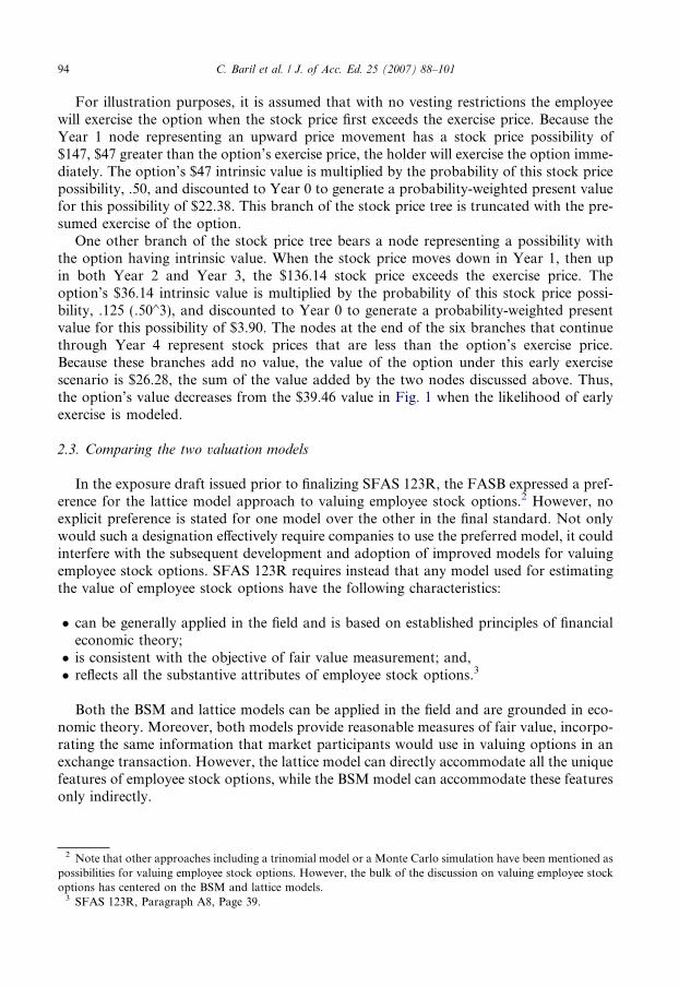
For illustration purposes, it is assumed that with no vesting restrictions the employeewill exercise the option when the stock price first exceeds the exercise price. Because theYear 1 node representing an upward price movement has a stock price possibility of$147, $47 greater than the option’s exercise price, the holder will exercise the option imme-diately. The option’s $47 intrinsic value is multiplied by the probability of this stock pricepossibility, .50, and discounted to Year 0 to generate a probability-weighted present valuefor this possibility of $22.38. This branch of the stock price tree is truncated with the pre-sumed exercise of the option.

One other branch of the stock price tree bears a node representing a possibility withthe option having intrinsic value. When the stock price moves down in Year 1, then upin both Year 2 and Year 3, the $136.14 stock price exceeds the exercise price. Theoption’s $36.14 intrinsic value is multiplied by the probability of this stock price possi-bility, .125 (.50�3), and discounted to Year 0 to generate a probability-weighted presentvalue for this possibility of $3.90. The nodes at the end of the six branches that continuethrough Year 4 represent stock prices that are less than the option’s exercise price.Because these branches add no value, the value of the option under this early exercisescenario is $26.28, the sum of the value added by the two nodes discussed above. Thus,the option’s value decreases from the $39.46 value in Fig. 1 when the likelihood of earlyexercise is modeled.

2.3. Comparing the two valuation models

In the exposure draft issued prior to finalizing SFAS 123R, the FASB expressed a pref-erence for the lattice model approach to valuing employee stock options.2 However, noexplicit preference is stated for one model over the other in the final standard. Not onlywould such a designation effectively require companies to use the preferred model, it couldinterfere with the subsequent development and adoption of improved models for valuingemployee stock options. SFAS 123R requires instead that any model used for estimatingthe value of employee stock options have the following characteristics:

� can be generally applied in the field and is based on established principles of financialeconomic theory;� is consistent with the objective of fair value measurement; and,� reflects all the substantive attributes of employee stock options.3

Both the BSM and lattice models can be applied in the field and are grounded in eco-nomic theory. Moreover, both models provide reasonable measures of fair value, incorpo-rating the same information that market participants would use in valuing options in anexchange transaction. However, the lattice model can directly accommodate all the uniquefeatures of employee stock options, while the BSM model can accommodate these featuresonly indirectly.

2 Note that other approaches including a trinomial model or a Monte Carlo simulation have been mentioned aspossibilities for valuing employee stock options. However, the bulk of the discussion on valuing employee stockoptions has centered on the BSM and lattice models.

3 SFAS 123R, Paragraph A8, Page 39.


To better understand this advantage of the lattice model it is useful to compare how thesubstantive characteristics of employee stock options are incorporated by each of the mod-els. When the underlying stock price exceeds the option’s exercise price, the fair value of anunexpired option consists of two components: intrinsic value and time value. In mostcases, an exchange-traded option is not exercised prior to expiration because the holderwould sacrifice the time value. Instead, the holder sells the exchange-traded option at aprice that incorporates this time value.

In contrast, employees often exercise their options prior to the end of the exercise per-iod. The holders forgo the time value of these options because they cannot be traded.Numerous compelling reasons have been advanced to explain why employees exercisetheir vested options early: lack of confidence in the company’s prospects, diversification,termination of employment, divorce, etc.

Early exercise behavior can be built into the lattice model directly using historical exer-cise patterns developed from company data. This behavior can be modeled to depend onthe stock price movement, how deep in the money the option is, and the length of timeuntil the option expires. Moreover, the lattice model can accommodate exercise behaviorthat varies over the term of the option.

Because the BSM model was developed for exchange-traded options assuming thatinvestors act optimally, it assumes that exercise occurs on the final day of the option’s con-tractual term. To incorporate the likelihood of early exercise, the BSM model must utilizea weighted-average life for the option rather than its contractual term. As an equation thatcan be solved for a given set of inputs, the closed form BSM model cannot directly accom-modate possible early exercise.

Another feature distinguishing employee stock options from exchange-traded optionsis their longer term, typically 10 years versus 90 days. The BSM model assumes thatboth the risk-free interest rate and the stock’s price volatility remain constant, anunreasonable assumption for employee options with 10-year terms. As a result, whenvaluing employee stock options using the BSM model, companies must input weightedaverages for the anticipated risk-free interest rate and volatility over the option’sweighted-average life. In contrast, the lattice model’s greater flexibility enables usersto assume different rates and volatilities for each time period. In fact, companies usingthe lattice model can incorporate different scenarios along selected paths of the stockprice tree.

Compared to the BSM model, the more adaptable lattice model should result in a bet-ter estimate of an option’s fair value. While commercial software is available for bothmodels, companies implementing a lattice model must make and document a numberof company specific assumptions and subjective judgments. For example, they mustextract and analyze historical data on the exercise behavior of employees holding optionsto specify and support the assumptions included in their models. And, while unable todirectly incorporate the substantive characteristics of employee stock options, companiesselecting the BSM model can do so indirectly by using the expected weighted averages asinputs.

Thus, the choice depends on the cost savings of the BSM model versus the likely supe-rior valuation estimate of the lattice model and the related financial statement impact. TheBSM model may provide a satisfactory valuation in cases where employee stock optionexpense is immaterial.


3. Option valuation project

This section describes a project requiring the use of Microsoft Excel to value a simpleemployee stock option with both the BSM and lattice models. Successfully employed atthe undergraduate (intermediate accounting) and graduate (accounting theory) levels,the project demonstrates the impact that changes in assumptions have on the fair valuesestimated. The project’s solution is presented followed by assessment data.

3.1. Microsoft Excel Project: Duke Dog Technologies

Lynn Malkani, a senior accountant in the Financial Reporting Department at DukeDog Technologies, has been assigned to assist the Controller, Tom Amico, with implemen-tation issues arising from the recently revised Statement of Financial Accounting StandardsNo. 123 (revised 2004) Share-Based Payment (FAS 123R). More specifically, Tom wouldlike Lynn to evaluate the feasibility of Duke Dog Technologies switching from valuing thecost of employee stock options using the Black–Scholes–Merton (BSM) option pricingmodel to using a lattice model.

Tom mentioned that from his understanding of the FASB’s deliberations leading up tothe issuance of the revised standard, the lattice model was considered a better approach forvaluing employee stock options than the BSM model. Tom said that as a ‘‘numbers’’ guy,he would like to see some computations, and he thought that by having Lynn do compu-tations using both models, she could gain some insight on how the models work and thenreport back to Tom with her thoughts on the merits of each approach.

Required:

1. Construct an Excel worksheet that calculates the value of a call option using the BSMmodel. Make sure the worksheet is correct by testing its calculations using the assump-tions from the example in Section 2.1. For simplicity calculate d1, d2, N(d1), N(d2) andC in progressive steps. Excel functions that will be helpful follow:� LN( ), returns the natural log function.� EXP( ), returns e raised to the power of that within the parentheses.� NORMSDIST( ), returns the standard normal cumulative distribution function.

2. Using the model you created in #1 above, calculate the value of a call option with thefollowing assumptions:

Stock price at date of grant
$80 Exercise price $80 Risk-free rate 4.5% Time to maturity 4 years Volatility 30% No dividends (a) What is the value of the call option with these assumptions? (b) What is the value of the option if volatility is increased to 40%?(c) What is the value of the option if volatility is decreased to 20%?(d) With the original volatility of 30%, what is the value of the option if time to
maturity is increased to 10 years?


(e) Using the original data, what is the value of the option when the risk free rate isdecreased to 3%?

3. Lattice approach. Construct a lattice model stock price tree in a new worksheet andvalue a call option using the following assumptions:

Stock price at date of grant
$80 Exercise price $80 Risk-free rate 4.5% Time to maturity 4 years Volatility 30% No dividends
Calculate the intrinsic value for each Year 4 node on the stock price tree. Next, prob-ability-weight the intrinsic values and determine their present values at Year 0. Finally,
aggregate these values to determine the option’s value at the grant date. Refer to Sec-tion 2.2 for further guidance.
4. The lattice model allows explicit consideration of the likelihood that option holders willexercise the option prior to its expiration date. Using the above assumptions, determinethe value of the option assuming that the option will be exercised whenever the stockprice exceeds the exercise price by 50% or more. Be sure to apply the appropriate num-ber of periods when discounting from the presumed exercise nodes.

5. Write a memorandum to Tom outlining your results in #1–4 above and then discuss thepros and cons of each employee stock option valuation approach.

3.2. Project solution

Requirements 1 and 2:

(a) What is the value of the call option with these assumptions? $24.65(b) What is the value of the option if volatility is increased to 40%? $29.95(c) What is the value of the option if volatility is decreased to 20%? $19.37(d) With the original volatility of 30%, what is the value of the option if time to maturity is

increased to 10 years? $40.78(e) Using the original data, what is the value of the option when the risk free rate is

decreased to 3%? $22.67

Requirement 3: option value: $24.07Requirement 4: option value with early exercise assumption: $22.48

Requirement 5:

Some of the key points to be included in the memorandum follow:

� Employee stock option value increases as volatility, time to maturity, and risk-free rateincrease.� Employee stock option value is most sensitive to changes in volatility and time to

maturity.� Advantages of the BSM model.� easier to implement,� less costly to implement.

Fig. 3. BSM model solution.


� Advantages of the lattice model.� allows for explicit consideration of the option being exercised prior to maturity,�more dynamic – allows for consideration of presumed changes in volatility and risk-

free rates over the option’s life.

3.3. Classroom assessment

As a means of assessing the effectiveness of the project, survey data were collected from46 undergraduate intermediate accounting students and 15 students in graduate account-ing theory. Exhibits 1 and 2 summarize the results. The survey instrument included sevenresponse items, each meant to capture the students’ level of understanding with respect toemployee stock options and the models used to estimate their fair value. Post-project datawere collected in the intermediate classes, while in the graduate theory class both pre- andpost-project data were collected. Students recorded their responses using a six-point Lik-ert-type scale.

Exhibit 1 summarizes the responses obtained from students in the undergraduate inter-mediate accounting classes. These students found that their levels of understanding withrespect to employee stock options, the BSM and lattice models, and the factors influencingvaluation increased by completing the project. For example, students indicated that theyagreed (4.96/6.0) with the fourth statement, ‘‘My understanding of the BSM option pric-ing model was increased by the case.’’

The responses received from students in the graduate theory class presented in Exhibit 2were consistent with those from the intermediate classes. The graduate theory studentsperceived the project as greatly improving their understanding of employee stock options,the BSM model, and the lattice model. For example, the average student response to

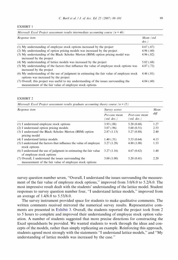
EXHIBIT 1

Microsoft Excel Project assessment results intermediate accounting course (n = 46)

Response item Mean (std.

dev.)

(1) My understanding of employee stock options increased by the project 4.67 (.67)(2) My understanding of option pricing models was increased by the project 4.96 (.60)(3) My understanding of the Black–Scholes–Merton (BSM) option pricing model was

increased by the project4.96 (.82)

(4) My understanding of lattice models was increased by the project 5.02 (.68)(5) My understanding of the factors that influence the value of employee stock options was

increased by the project4.87 (.72)

(6) My understanding of the use of judgment in estimating the fair value of employee stockoptions was increased by the project

4.46 (.81)

(7) Overall, this project was useful to my understanding of the issues surrounding themeasurement of the fair value of employee stock options

4.84 (.60)

EXHIBIT 2

Microsoft Excel Project assessment results graduate accounting theory course (n = 15)

Response item Survey scores Mean

diffPre-case mean

(std. dev.)

Post-case mean

(std. dev.)

(1) I understand employee stock options 3.93 (.88) 5.20 (0.68) 1.27(2) I understand option pricing models 3.07 (.96) 5.60 (0.51) 2.53(3) I understand the Black–Scholes–Merton (BSM) option

pricing model2.87 (1.13) 5.27 (0.88) 2.40

(4) I understand lattice models 1.40 (.51) 5.53 (0.64) 4.13(5) I understand the factors that influence the value of employee

stock options3.27 (1.28) 4.80 (1.08) 1.53

(6) I understand the use of judgment in estimating the fair valueof employee stock options

3.27 (1.16) 4.67 (0.62) 1.40

(7) Overall, I understand the issues surrounding themeasurement of the fair value of employee stock options

3.00 (1.00) 5.20 (0.41) 2.20


survey question number seven, ‘‘Overall, I understand the issues surrounding the measure-ment of the fair value of employee stock options,’’ improved from 3.0/6.0 to 5.2/6.0. Themost impressive result dealt with the students’ understanding of the lattice model. Studentresponses to survey question number four, ‘‘I understand lattice models,’’ improved froman average of 1.4/6.0 to 5.53/6.0.

The survey instrument provided space for students to make qualitative comments. Thewritten comments received mirrored the numerical survey results. Representative com-ments are presented in Exhibit 3. Overall, the students reported the project took from 2to 5 hours to complete and improved their understanding of employee stock option valu-ation. A number of students suggested that more precise directions for constructing theExcel spreadsheets be provided. We wanted students to work through the ideas and con-cepts of the models, rather than simply replicating an example. Reinforcing this approach,students agreed most strongly with the statements ‘‘I understand lattice models,’’ and ‘‘Myunderstanding of lattice models was increased by the case.’’

EXHIBIT 3

Microsoft Excel Project selected written student comments

Undergraduate intermediate course

‘‘The case definitely broadened my knowledge about stock options. Before this assignment I was clueless aboutthe different factors that go into stock options; now I have a better understanding.’’

‘‘My understanding of stock options definitely increased but it was still a little rocky getting there. It wouldhave been nice to see some actual examples of how these processes are done, rather than going in completelyfresh.’’

‘‘I think the project was useful. It allowed us to use them and understand how things affect the models. It alsohelped me understand why a company would use a certain model over another.’’

‘‘Excel programming a little tricky, but other than that a fine project.’’

Graduate theory course

‘‘The case was quite interesting to complete. I definitely learned much more about both models than I had in someprevious classes. The actual application process – constructing the models in Excel – was quite difficult though,but satisfying in the end. More clear cut and precise directions to create the models in Excel would be great.Overall, it was a challenging but good learning project.’’

‘‘Took about 2–3 h to complete; writing the memo brought everything together.’’‘‘Spent about 3 h total on the case. Excel assignments were very helpful to understand what goes on in the BSM

model and how variables affect value. Better explanation of the lattice model would have helped (with anexample).’’


4. Summary

Estimating the fair value of employee stock options for purposes of recording compen-sation expense represents one of the greatest challenges in implementing SFAS 123R. Theconceptual discussion coupled with illustrated examples of stock option accounting andvaluation will enhance student understanding of the issues.

Appendix. Accounting for stock options

The following example illustrates the accounting for employee stock options underSFAS 123R. On January 1, 2006, Duke Corporation grants 100 options to an employee.The options have an exercise price of $10, the same as the stock price on the grant date.Further, the options vest at the end of three years, expire after 10 years, and have an esti-mated fair value on the grant date of $450 (100 options · $4.50/option). Because all theoptions are expected to vest, a total compensation expense of $450 is recognized evenlyover the three-year service period, 2006–2008, the period between grant and vesting duringwhich the employee will perform services. Accordingly, Duke Corporation will make thefollowing journal entry at the end of each year.

12/31/06
Compensation expense $150
Paid-in capital-stock options
$150 (To recognize annual compensation expense: $450/3 years)
No liability is reported because the company is not obligated to sacrifice cash or otherassets when the stock options are exercised.


Next, assume that the employee exercises the options on January 31, 2009 when thestock price is $30 per share. If Duke Corporation’s common stock is no-par stock, itrecords the exercise as follows:

1/31/09
Cash ($10 exercise price · 100 options) $1000
Paid-in capital-stock options (account balance)
450
No-par common stock
$1450
(To record the issuance of stock upon exercise of options)

Because compensation expense is not continually adjusted to reflect changes in the mar-ket price of the stock, the stock’s price at the exercise date does not impact this journalentry. While the opportunity cost is $2000, the difference between the $3000 ($30/share · 100 shares) market price of the shares on the exercise date and the cash received,Duke’s total compensation expense remains unchanged at $450 as measured at the grantdate.

If the employee chooses instead to let the options expire, Duke Corporation wouldmake the following journal entry:

12/31/15
Paid-in capital-stock options (account balance) $450
Paid-in capital-expired stock options
$450
(To record the expiration of stock options)

The employee would let the options lapse if the stock’s price failed to rise above theoption’s exercise price during the exercise period. The journal entry simply re-titles DukeCorporation’s paid-in capital. As is the case when the options are exercised, the company’scompensation expense is unaffected by the expiration of the options.

This example assumes that Duke Corporation’s stock option plan qualifies as an incen-tive plan. Because the company receives no deduction upon exercise of the options, thereare no tax consequences. Alternatively, if the plan does not qualify as an incentive plan,Duke must recognize a deferred tax asset along with compensation expense, reflectingthe temporary difference between accounting and tax income. If the eventual tax savings,the market value of the shares issued upon exercise less the cash received from the optionholder, differs from the deferred tax asset created, the difference is recognized as equity.

Reference

Financial Accounting Standards Board (2004). Share-based payments (SFAS 123R). Statement of financial

accounting standard no. 123 (revised 2004). Norwalk, CT: FASB.

valuing employee stock options under sfas 123r using the black–scholes–merton and lattice model...

Documents