values of time for carpool commuting with hov lanes: a

HAL Id: halshs-02988756https://halshs.archives-ouvertes.fr/halshs-02988756

Preprint submitted on 6 Nov 2020

HAL is a multi-disciplinary open accessarchive for the deposit and dissemination of sci-entific research documents, whether they are pub-lished or not. The documents may come fromteaching and research institutions in France orabroad, or from public or private research centers.

L’archive ouverte pluridisciplinaire HAL, estdestinée au dépôt et à la diffusion de documentsscientifiques de niveau recherche, publiés ou non,émanant des établissements d’enseignement et derecherche français ou étrangers, des laboratoirespublics ou privés.

Values of Time for Carpool Commuting with HOVlanes: A Discrete Choice Experiment in France

Alix Le Goff, Guillaume Monchambert, Charles Raux

To cite this version:Alix Le Goff, Guillaume Monchambert, Charles Raux. Values of Time for Carpool Commuting withHOV lanes: A Discrete Choice Experiment in France. 2020. �halshs-02988756�

https://halshs.archives-ouvertes.fr/halshs-02988756

https://hal.archives-ouvertes.fr

www.laet.science.fr

WORKING PAPERS DU LAET

NUMÉRO 2020/02

Values of Time for Carpool Commuting with HOV lanes: A Discrete Choice Experiment in France

Alix LE GOFF

Guillaume MONCHAMBERT

Charles RAUX

We conduct a discrete choice experiment on 931 solo-driving commuters in Lyon, France to estimate the values of end-to-end travel time (VoTT) in the presence of an HOV lane for four modes: Solo Driver, Carpool Driver, Carpool Passenger and Public Transport. Mixed and latent class logit models are estimated. We find that Carpool Passenger, Carpool Driver and Public Transport median VoTTs are respectively around 20%, 40% and 60% higher than Solo Driver VoTT. The analysis of individual heterogeneity distinguishes three classes of behavior in our sample: open to carpool as a driver (41%), open to passenger modes (32%) and resistant to all alternatives to solo driving (28%). These three categories allow to identify solo drivers who could switch to carpool as drivers. We show that encouraging current solo drivers to switch to carpool as passengers will be more sensitive if public transport services are also improved.

Keywords: Values of Time, Carpool, Commuting Trips, HOV-lane, Discrete Choice Experiment

J.E.L. Classification: R41, C35

Avertissement Les Working Papers du LAET n’ont pas vocation à être une revue. En conséquent, ils ne sont

pas dotés d’un comité éditorial et les propos n’engagent que leur(s) auteur(s) avec ou sans review.

Sans review Ce WP n’a pas fait l’objet d’une review par ses pairs. Les propos n’engagent que son ou ses auteur(s).

Avec review Ce WP a fait l’objet d’une review par ses pairs en guise d’amélioration du contenu et non de contrôle éditorial. Les propos n’engagent que son ou ses auteur(s).

NUMÉRO 2020/02

Values of Time for Carpool Commuting with HOV lanes: A Discrete Choice Experiment in France

Alix LE GOFF Univ Lyon, Université Lyon 2, LAET, F‐69007, LYON, France

Guillaume MONCHAMBERT Univ Lyon, Université Lyon 2, LAET, F‐69007, LYON, France

Charles RAUX Univ Lyon, CNRS, LAET, F‐69007, LYON, France

2020 Laboratoire Aménagement Économie Transports MSH Lyon St-Etienne 14, Avenue Berthelot F-69363 Lyon Cedex 07 France

A. Le Goff, G. Monchambert, C. Raux

1

Values of Time for Carpool Commuting with HOV-lanes: A Discrete Choice 1

Experiment in France 2

Alix Le Goff1

Université de Lyon, Université Lyon 2, LAET, F‐69007, LYON, France

Guillaume Monchambert

Université de Lyon, Université Lyon 2, LAET, F‐69007, LYON, France

Charles Raux

Université de Lyon, CNRS, LAET, F‐69007, LYON, France

ABSTRACT 3

We conduct a discrete choice experiment on 931 solo-driving commuters in Lyon, France to estimate 4

the values of end-to-end travel time (VoTT) in the presence of an HOV lane for four modes: Solo Driver, 5

Carpool Driver, Carpool Passenger and Public Transport. Mixed and latent class logit models are 6

estimated. We find that Carpool Passenger, Carpool Driver and Public Transport median VoTTs are 7

respectively around 20%, 40% and 60% higher than Solo Driver VoTT. The analysis of individual 8

heterogeneity distinguishes three classes of behavior in our sample: open to carpool as a driver (41%), 9

open to passenger modes (32%) and resistant to all alternatives to solo driving (28%). These three 10

categories allow to identify solo drivers who could switch to carpool as drivers. We show that 11

encouraging current solo drivers to switch to carpool as passengers will be more sensitive if public 12

transport services are also improved. 13

Keywords: Values of Time; Carpool; Commuting Trips; HOV-lane; Discrete Choice Experiment 14

15

Declarations of interest: none 16

1 Corresponding Author

Email: [email protected]


2

1. INTRODUCTION 1

Traffic congestion is still a major issue in large cities around the world. France is no exception to this 2

observation. According to INRIX (2018), the drivers in Paris, Marseille, Lyon and Toulouse – the four 3

largest cities in the country – respectively lost on average 237, 140, 141 and 130 hours in road congestion 4

in 2018. Most of this traffic congestion appears during morning and evening peak hours. 5

Promoting carpool is seen as a cost-effective way to moderate road congestion while avoiding costly 6

investments in road expansion and also to reduce harmful gas emissions. As USA recently experienced 7

an increase in solo driving in commuting modal share (AASHTO, 2013), the objective here is to increase 8

car occupancy rate. There is a clear room for improvement as the current rate is low in France, between 9

1.2 and 1.3 individuals per vehicle on average for weekday trips (ENTD, 2008). This occupation rate 10

falls at 1.08 for commuting trips. Similar results are found in UK2, USA3 or Australia4. It implies that 11

there is a large unused transport capacity during peak hours. 12

Local policy makers in France currently consider different kinds of policies to promote carpool for 13

commuting trips. The cities of Lyon and Grenoble are expected to experiment HOV-lanes in 2020. These 14

lanes are expected to reduce travel time and to increase travel time reliability for carpoolers. The Ile-de-15

France (Paris) Region gives monetary incentives to carpool drivers (between 1.5 and 3 euros per trip), 16

and free public transport tickets for carpool passengers. Several regions have developed a carpool web 17

platform to ease the matching between drivers and passengers. Private companies are also encouraging 18

their employees to carpool. Moreover, Vinci, a toll motorway company, has launched a partnership with 19

Blablacar, the world number one carpool company (see Shaheen et al. 2017). Vinci’s subscribers 20

carpooling on the motorway benefit from lower management fees on the BlaBlaCar platform. 21

Promoting a successful carpool policy needs a better understanding and measure of carpool trips 22

attributes. In a state-of-the-art of ridesharing5, Furuhata et al. (2013) emphasized how route and time 23

matching issues between drivers and passengers can be very constraining, even in a simple situation. 24

They also identify different classes of carpools/rideshares and hence different constraints and/or 25

advantages for each one. Chaube et al. (2010) conducted a survey in an American university and found 26

that a close relationship between carpoolers was a key factor of successful ride-matching: 98% of 27

students would accept to carpool with a friend, 69% with a friend of a friend, but only 7% would accept 28

a ride with a person they do not know. Gender and age differences in the car party are also issues 29

involved. However, in spite of several studies identifying obstacles to carpool, we did not find evidences 30

of carpool-specific values of travel time in the literature. 31

This paper aims to fill this gap. We address the following research questions: what are the values of 32

travel time (VoTT) as a carpool driver or passenger? Are these values different from the values for a 33

2https://assets.publishing.service.gov.uk/government/uploads/system/uploads/attachment_data/file/457752/nts20

14-01.pdf 3 https://nhts.ornl.gov/2009/pub/stt.pdf 4 https://chartingtransport.com/2011/08/20/whats-happening-with-car-occupancy/ 5 In the following we use indifferently “carpooling” or “ridesharing”.

https://nhts.ornl.gov/2009/pub/stt.pdf

https://webmail.cnrs.fr/owa/redir.aspx?C=DsPdxzfy462IvupLogAL-rOeImj7SSRscR8GRxpMg5dUhEMQClTYCA..&URL=https%3a%2f%2fchartingtransport.com%2f2011%2f08%2f20%2fwhats-happening-with-car-occupancy%2f


3

trip made as a solo driver or a public transport user? How are the values distributed across the commuter 1

population? 2

We answer these questions by estimating end-to-end VoTT and their distributions for commuting trips 3

as a solo driver, a carpool driver, a carpool passenger and a public transport passenger. End-to-end travel 4

time (or total travel time) are valued in this paper to compare values found for carpool to the existing 5

values for car. This choice is made even though times can be valued differently in a trip – like walk or 6

wait – like Wardman (2016) showed for public transport. To this aim, a discrete choice experiment 7

survey is conducted on a sample of 931 commuters using their car to commute in the city of Lyon. We 8

use mixed and latent class logit models to consider the panel structure of our data and the heterogeneity 9

of commuters. 10

Results are of interest for several reasons. To our knowledge, we are the first to empirically measure 11

and valuate the time attributes of carpool commuting and to compare these values with those for usual 12

modes. Hence, this paper contributes to the literature by estimating mode-specific values of time. 13

Furthermore, the analysis of individual heterogeneity could allow public policies to target the profiles 14

of drivers most likely to switch from solo driving to carpooling and provide information on potential 15

subsidies to encourage this switch. We produce estimations of carpool-specific values of time which can 16

be used in transport forecasting models. They could also be used as prior values to establish official 17

guidelines in cost-benefit analysis. Finally, carpool matching platforms could be interested in our 18

estimations and in our latent class models to implement market differentiation. 19

The rest of the paper is organized as follows. Section 2 below is a literature review of carpooling issues 20

and VoTT surveys. Section 3 presents the survey design, data sampling and summary statistics. Section 21

4 shows the methodological framework and the empirical strategy used to estimate values of time. 22

Section 5 presents the results, which are discussed in Section 6 and Section 7 concludes. 23

2. LITERATURE REVIEW 24

2.1 Carpool for commuting and HOV-lanes 25

Even though the French company Blablacar substantially promoted carpooling for long distance trips, 26

this mode is still rarely used in France on a daily basis6. Several constraints may explain this fact. 27

The matching process appears to be more difficult for daily carpool than it is for occasional long-distance 28

carpool trips. More specifically, compared to long-distance carpool, schedule and spatial (i.e. nearby 29

origins and nearby destinations) constraints in daily carpool have an increased role in the matching 30

between driver and passenger. As the trip is shorter than in long distance, detour time, waiting time, 31

access or egress times represent a higher part of the end-to-end travel time. So, the temporal and spatial 32

match between a driver and a passenger has to be almost perfect to avoid this time loss. In a 33

state-of-the-art on ridesharing, Furuhata et al. (2013) showed how quickly matching can be problematic 34

when a driver and several passengers have to match at different times and places. They show that optimal 35

6 The modal share of carpooling for medium-distance commuting (20 to 80 km) in France is estimated around

10% (ADEME, 2015)


4

matching situations (which allow each passenger to find a driver and vice versa) are not always easily 1

achievable. 2

In addition to these matching issues and similarly to long-distance carpool, daily carpooling raises the 3

question of trust between carpoolers. Trust is a key element to give or take rides from others (Chaube et 4

al., 2010). Chan & Shaheen (2012) made a review of ridematching programs in North America. 5

Individuals often consider carpooling as a risky mode. The desire of independency or flexibility are also 6

reasons raised from solo drivers to stay alone in their car (Li et al., 2007). 7

In a Texan survey (Li et al., 2007) and a French survey (ADEME, 2015), carpoolers often cite 8

friendliness, ecology or a reduced stress and fatigue – in addition to economic criteria – as reasons why 9

they choose this mode. Intuitively, the economic gain or loss is an essential attribute in the transport 10

modal choice. Sharing the costs makes carpooling economically competitive compared to solo driving. 11

Some incentives can also make individuals change their transport mode choice, like “parking cash-out” 12

experienced in California Shoup (1997), or “positive toll” concept tested in Rotterdam7. Results showed 13

an increase of carpoolers in the first experiment and a reduction of traffic in the second. 14

Another incentive to carpool is to implement lanes reserved to high occupancy (HOV) lanes which offer 15

time savings to carpoolers. Necessary criteria for their proper functioning have been mentioned by 16

Schijns & Eng (2006) and Chan & Shaheen (2012). The HOV-lane has to be used by an important 17

number of people to avoid the “empty lane” phenomenon and to gain acceptance from the population. 18

It should give significant and reliable travel-time savings. An efficient HOV-lane should increase the 19

number of people using the corridor. Several studies showed these lanes can be effective, like in New 20

York where Ugolik et al. (1996) measured HOV-lanes increased the number of people in the vehicles 21

by 14%. In their survey and focus groups, they also found both HOV users and non-users support an 22

extension of the HOV-lane. Other surveys also demonstrate HOV-lanes can have a positive impact on 23

traffic too. Traffic measurements on several HOV¬ lanes in San Francisco Bay Area conducted by 24

Daganzo & Cassidy (2008) show that HOV-lanes that does not create new bottlenecks add very few 25

vehicular delay (i.e. the average time spent crossing the corridor), around 2% and reduce people delay 26

by more than 10%. 27

These past results suggest public policies should focus on three main attributes to convince people to 28

carpool: monetary gains, time savings and building trust. 29

2.2 Values of Travel Time Heterogeneities 30

Sensitivities for monetary gains and time savings and more precisely their ratio (value of travel time, 31

VoTT) are very discussed in the transport economics literature. This high consideration is due to their 32

usage in both the evaluation of transport projects - to calculate the social welfare - and also the 33

understanding of individual's mode or route choices. In a paper entirely devoted to VoTTs, Small (2012) 34

discussed VoTT heterogeneity found in the literature. This heterogeneity depends on various elements 35

such as trip purpose, discomfort in a transportation mode, traffic conditions, trip duration. However, this 36

7 https://www.rse-egis.fr/en/solution_egis/positive-tolls/


5

paper suggests that a wide part of these heterogeneities remains misunderstood and hence depends on 1

individual unobserved characteristics. 2

The empirical results show indeed a large heterogeneity in VoTTs: Jara-Diaz et al (2008) showed 3

through an analysis of work and leisure in three different countries (Chile, Switzerland and Germany), 4

that the commuting VoTT is not the same between different countries. These results are confirmed by a 5

worldwide meta-analysis proposed by Shires & De Jong (2009) and European meta-analyses (see 6

Wardman et al. 2012, 2016). Their results suggest that VoTT is correlated less than proportionally to 7

wage rate with income elasticities varying between 0.68 and 0.85. The heterogeneity of VoTT found in 8

their different studies also depends on trip purpose and traffic conditions, they are higher in congested 9

conditions than in free flow. 10

VoTTs appear heterogeneous also depending on the mode. Wardman et al. (2016) distinguished mode 11

used – relative to individual characteristics – and mode valued – relative to mode characteristics such as 12

comfort, privacy, security or externalities due to environment. Their findings show a mode valued 13

difference between bus and car for commuting trips, with a significantly lower VoTT in car trips. 14

Previous surveys tend to show that travel time values are lower for public transport users – in bus and 15

rail – than for car users (Shires & De Jong, 2009; Wardman et al., 2012; Quinet, 2013). With regard to 16

carpooling VoTT, in a SP survey, Blayac & Adjeroud (2018) compared VoTTs of bus and carpool users 17

over long distances. They found that the value of time for carpool users is more than twice the one of 18

bus users. Monchambert (2020), in a long-distance carpool survey, founds that VoTTs in carpooling are 19

higher than those as a solo driver, bus user and train user. 20

Different modeling techniques are used to capture the individual heterogeneity. The most common is to 21

use a mixed logit model that allows some attribute coefficients to be distributed throughout the 22

population (e.g. Hess et al., 2005). In our case, cost and time individual sensitivities are examined to 23

determine VoTT. However, several issues may appear as shown in Daly et al (2012) to determine the 24

ratio of two distributions. A solution is to use WTP space (see Train & Weeks, 2005) to solve the 25

problem. Multiplying the cost coefficient with time coefficients allows to estimate only one distribution. 26

Other discrete choice models allow alternative evaluations of heterogeneity and may simplify their 27

interpretation. A complementary modelling and interpretation of individual heterogeneity can be 28

provided through a latent class logit model, in which the sample is considered as represented by several 29

classes, each one having different sensitivities (see e.g. Greene and Hensher, 2003; Shen et al., 2006). 30

3. SURVEY DESIGN AND DATA SAMPLING 31

A discrete choice experiment is designed to collect data to examine the trade-off between travel time, 32

delays and cost (or gain) for trips as a driver or as a passenger. This experiment has been conducted 33

through a responsive questionnaire described below. 34


6

3.1 Study context 1

This questionnaire was designed to observe how the inhabitants of the Lyon area (1.4M inhabitants) 2

would react to the creation of a HOV-lane, a new infrastructure in France8. Indeed, the City of Lyon is 3

going to set up two HOV-lane sections on its main North-South axis, allowing shorter and more reliable 4

travel times for carpoolers than for solo drivers. These lanes will be 6 and 4-km long for the northern 5

and the southern sections respectively. The expected time savings for carpoolers are between 5 and 10 6

minutes during morning rush hours. 7

3.2. Survey design 8

The questionnaire is organized in three parts. The first part aims at collecting basic socio-demographic 9

data and the trip characteristics. The second part is the stated choice experiment. It is a dynamic 10

experiment in the sense that the choices tasks proposed to the respondent depend on her trip 11

characteristics. The third part is a questionnaire on attitudes. 12

First part: socio-demographic and trip characteristics 13

We first collect information on socio-economics variables of the respondent (gender, age, income, 14

professional position…) and on the characteristics of their “usual trip” i.e. the most frequent trip made 15

by public transport or car. These characteristics will be used to responsively build the choice tasks in 16

the second step of the survey. 17

Our aim is to place the respondent in the context of a trip he can do with the proposed modes in the 18

survey. For very short distance trips (<15 minutes by car), we consider carpooling is not a credible 19

alternative. Even a short waiting time (for the passenger) or detour time (for the driver) would 20

proportionally lengthen the trip a lot. On the other hand, trips longer than 90 minutes were also 21

considered as too long for carpooling, the time gain procured by the HOV-lane could be proportionally 22

too short to be convincing to change mode. Furthermore, the average commuting time by car in Lyon 23

area is around 30 minutes9 and the longer the trip the harder it would be to find a carpooler far from the 24

city center. Consequently, only respondents whose usual trip meets the following criteria are kept in the 25

survey: 26

- a travel time between 15 and 90 minutes 27

- driving their car 28

- during rush hours (between 6 and 10 am or between 4 and 8 pm, excluding weekends) 29

The respondent is then randomly assigned to one of two kinds of carpool organization (planned or 30

spontaneous). Planned carpool implies meeting place and time schedule arranged before the trip starts. 31

8 As HOV-lane is not a common infrastructure in France, we introduced in the survey a screen presenting this

infrastructure. 9 We remind the average commuting time by car is inferior to 30 minutes in Lyon : https://www.scot-

rivesdurhone.com/wp-

content/uploads/2016/08/EnqDeplcmt2015_plaq_generale_27062016_120dpi_pourWEB.pdf


7

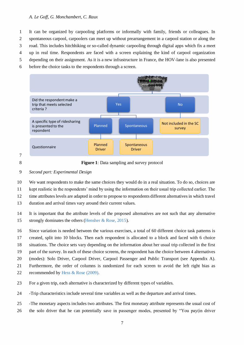
It can be organized by carpooling platforms or informally with family, friends or colleagues. In 1

spontaneous carpool, carpoolers can meet up without prearrangement in a carpool station or along the 2

road. This includes hitchhiking or so-called dynamic carpooling through digital apps which fix a meet 3

up in real time. Respondents are faced with a screen explaining the kind of carpool organization 4

depending on their assignment. As it is a new infrastructure in France, the HOV-lane is also presented 5

before the choice tasks to the respondents through a screen. 6

7

Figure 1: Data sampling and survey protocol 8

Second part: Experimental Design 9

We want respondents to make the same choices they would do in a real situation. To do so, choices are 10

kept realistic in the respondents’ mind by using the information on their usual trip collected earlier. The 11

time attributes levels are adapted in order to propose to respondents different alternatives in which travel 12

duration and arrival times vary around their current values. 13

It is important that the attribute levels of the proposed alternatives are not such that any alternative 14

strongly dominates the others (Hensher & Rose, 2015). 15

Since variation is needed between the various exercises, a total of 60 different choice task patterns is 16

created, split into 10 blocks. Then each respondent is allocated to a block and faced with 6 choice 17

situations. The choice sets vary depending on the information about her usual trip collected in the first 18

part of the survey. In each of these choice screens, the respondent has the choice between 4 alternatives 19

(modes): Solo Driver, Carpool Driver, Carpool Passenger and Public Transport (see Appendix A). 20

Furthermore, the order of columns is randomized for each screen to avoid the left right bias as 21

recommended by Hess & Rose (2009). 22

For a given trip, each alternative is characterized by different types of variables. 23

-Trip characteristics include several time variables as well as the departure and arrival times. 24

-The monetary aspects includes two attributes. The first monetary attribute represents the usual cost of 25

the solo driver that he can potentially save in passenger modes, presented by “You pay(in driver 26

Questionnaire

A specific type of ridesharing is presented to the repondent

Did the respondent make a trip that meets selected criteria ?

Yes

Planned

Planned Driver

Spontaneous

Spontaneous Driver

No

Not included in the SC survey


8

modes)/save on(in passenger modes) your usual transportation cost” in the choice screens. The second 1

attribute is the price paid for a ride in public transport or in carpool as a passenger. It may also represent 2

the gain earned in carpool as a driver. 3

-In carpool alternatives, matched carpooler’s profile is also presented in order to check for other 4

attributes who could affect mode choice such as close relationship between driver and passenger. Even 5

though these variables are expected to affect mode choice, we will mainly focus on time and monetary 6

aspects in this paper. 7

The Ngene software (ChoiceMetrics, 2012) is used with a D-efficient design (see Rose et al., 2008) to 8

build balanced choice tasks without dominated or dominant alternatives. The efficient design allows to 9

avoid strong dominance of one mode on another. For that, prior information about parameters have been 10

used from de Palma and Fontan (2000) and Quinet (2013). The mode attributes and levels used in the 11

choice tasks are presented in Table 1. 12

13

Table 1: Trip attributes and levels in stated choice design 14

Attributes Alternatives Levels

Time variables

Schedule early/late Solo Driver 0, 30, 60 minutes (earlier or later)

End-to-end travel time

(in min)

Solo Driver

Carpool Driver

Carpool Passenger

Public Transport

Min: 0.8 * usual_tt Max: 1.9 * usual_tt

Min: 0.6 * usual_tt Max: 1.5 * usual_tt + 20

Min: 0.6 * usual_tt + 10 Max: 1.5 * usual_tt + 50

Min: 0.6 * usual_tt + 10 Max: 1.5 * usual_tt + 35

Cost (in €)

Carpool Driver

Carpool Passenger

Public Transport

Receives (0, 0.02, 0.05, 0.1) * usual_tt

Pays (0, 0.02, 0.05, 0.1) * usual_tt

Pays 0.8

Carpooler profile

Carpooler matching Carpool Driver and

Carpool Passenger Planned, Spontaneous

Carpooler Gender Male, Female

(not presented if relative)

Carpooler Age 25, 45, 65 years old


Notes: Passenger modes: Carpool Passenger and Public Transport. Carpool modes: Carpool Driver and

Carpool Passenger. “usual_tt” is the usual travel time the respondent reports in the survey. Detailed attribute

levels are provided in Appendix D.

15

Third part: Attitude Questions 16

Finally, five questions are asked to evaluate the respondent’s sensitivity to environmental consequences 17

of the solo driving practice. Indeed, incentivizing carpooling involves psychological and social 18

dimensions which go beyond self-interest, this latter dimension being covered through our DCE design. 19


9

The environment or the level of congestion in the city may be seen as “commons” which deserve specific 1

behavioral adaptations. 2

Regarding the potential of motivational factors towards pro-environmental behavior, the literature offers 3

two main theories. The one is based on self-perceived cost and benefits, with the theory of planned 4

behavior (TPB; Ajzen, 1991). TPB aims at explaining behavioral intentions (viewed as the immediate 5

antecedent of actual behavior) by the attitudes (ATT), the perceived social pressure regarding this 6

behavior (subjective norms, SN) and the perceived behavioral control (PBC). The other theory is based 7

on moral and normative concerns with the norm-activation theory (NAT; Schwartz, 1977) and aims at 8

explaining altruistic behavior. Feelings of obligation, stemming from perceived norms (PN), precede 9

immediately behavior and are activated by the awareness of behavior consequences (AC) and beliefs 10

about personal responsibility. 11

These two theories are applied and compared by Wall et al. (2007) in order to explain drivers’ intentions 12

to reduce or maintain their car use for commuting. The authors show that a combination of TPB and 13

NAT constructs has a superior power of explanation when compared to the two theories separated. 14

Following Wall et al. conclusions we build a set of five statements (presented on a Likert scale) which 15

cover the basic constructs of both theories: 16

1: Car traffic is a major source of pollution and congestion (AC). 17

2: I am satisfied with my daily trip choices (ATT). 18

3: I can or could easily change the way I travel on a daily basis (PBC). 19

4: The opinion of people who matter to me is important for the way I travel on a daily basis (SN). 20

5: I feel personally responsible for contributing to reduce pollution and congestion (PN). 21

3.3. Data 22

Data was collected from an online survey. A partnership with different motorway companies, local 23

authorities, University of Lyon and a carpool-specialized company allowed us to spread a web-link of 24

the survey to many inhabitants in the Lyon area. There was a financial incentive to answer the survey 25

as respondents had a chance to win a 100€ voucher. A wide part of the sample came thanks to the 26

dissemination of the survey to electronic tolling motorway subscribers. Finally, a database containing 27

around 3,300 respondents who fully completed the survey was collected. 28

In this paper our focus is on the potential change of daily commuters from solo-driving to carpooling 29

when facing an HOV-lane. Thus, only respondents who declare an usual trip as solo drivers, at least 30

several times a week and for work purpose are kept. This commuters’ subset still represents an important 31

part of our base sample, with 2,044 respondents. 32

Finally, some adhoc data filtering is applied as recommended by Hess et al. (2010). Since response times 33

for each choice screen are available, people who answered to a choice screen at least once in less than 6 34

seconds are excluded. This allows us to remove respondents who only came to win a voucher and answer 35


10

the questionnaire as fast as they can without examining the choice sets. Furthermore, we considered as 1

our respondents are currently solo drivers, they should at least select Solo Driver mode once, to get close 2

from their revealed preferences. This filtering is detailed in Appendix C. 3

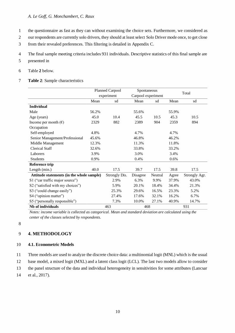
The final sample meeting criteria includes 931 individuals. Descriptive statistics of this final sample are 4

presented in 5

Table 2 below. 6

Table 2: Sample characteristics 7

Planned Carpool

experiment

Spontaneous

Carpool experiment Total

Mean sd Mean sd Mean sd

Individual

Male 56.2% 55.6% 55.9%

Age (years) 45.0 10.4 45.5 10.5 45.3 10.5

Income per month (€) 2329 882 2389 904 2359 894

Occupation

Self-employed 4.8% 4.7% 4.7%

Senior Management/Professional 45.6% 46.8% 46.2%

Middle Management 12.3% 11.3% 11.8%

Clerical Staff 32.6% 33.8% 33.2%

Laborers 3.9% 3.0% 3.4%

Students 0.9% 0.4% 0.6%

Reference trip

Length (min.) 40.0 17.5 39.7 17.5 39.8 17.5

Attitude statements (in the whole sample) Strongly Dis. Disagree Neutral Agree Strongly Agr.

S1 (“car traffic major source”) 2.9% 6.3% 9.9% 37.9% 43.0%

S2 (“satisfied with my choices”) 5.9% 20.1% 18.4% 34.4% 21.3%

S3 (“could change easily”) 25.3% 29.6% 16.5% 23.3% 5.2%

S4 (“opinion matter”) 27.4% 17.6% 32.1% 16.2% 6.7%

S5 (“personally responsible”) 7.3% 10.0% 27.1% 40.9% 14.7%

Nb of individuals 463 468 931

Notes: income variable is collected as categorical. Mean and standard deviation are calculated using the

center of the classes selected by respondents.

8

4. METHODOLOGY 9

4.1. Econometric Models 10

Three models are used to analyze the discrete choice data: a multinomial logit (MNL) which is the usual 11

base model, a mixed logit (MXL) and a latent class logit (LCL). The last two models allow to consider 12

the panel structure of the data and individual heterogeneity in sensitivities for some attributes (Lancsar 13

et al., 2017). 14


11

Multinomial Logit (MNL) 1

The probability to choose j among the K alternatives available for individual i in MNL can be written: 2

Pij =exp(Xijβj)

∑k=1K exp(Xikβk)

3

where X designate characteristics of the observable part of the utility and βk are the model’s estimates 4

for alternative k. 5

Nonetheless, this model has some limitations such as the Independence of Irrelevant Alternatives (IIA) 6

assumption. Therefore, MXL and LCL models have been proposed in the literature to allow for 7

individual heterogeneity between the respondents and to release the IIA assumption (see e.g. McFadden 8

& Train, 2000; Greene & Hensher, 2003). 9

Mixed Multinomial Logit (MXL) 10

The MXL model allows for heterogeneity through “random parameters” estimates the analyst can 11

define. The difference with the MNL is that the βk estimates become βik, varying through individuals 12

and following a distribution chosen by the analyst. 13

Following Train (2009) the mixed logit probabilities are the integrals of standard logit probabilities over 14

a density of parameters. 15

Pij = ∫Lij(β)f(β)dβ 16

where f(β) is a density function and Lij(β) the logit probability evaluated at β such that 17

Lij(β) =exp(Vij(β))

∑ exp(Vik(β))k 18

This specification is extended to take account of T repeated choices by each individual in the sample. 19

The utility for individual i in choice situation t becomes: 20

Uijt = βijXijt + εijt 21

and 22

Pij = ∫∏exp(βijXij)

∑ exp(βikXik)k

T

t=1

f(β)dβ 23

We assume individuals cannot enjoy travelling longer. Hence, lognormal distributions are estimated for 24

all time attributes to avoid negative values of time. 25

(1)

(2)

(3)

(4)

(5)


12

Latent Class Logit (LCL) 1

Contrary to the MXL, the LCL model does not need any assumption on distribution of preferences in 2

the population. This model assumes that the sample is implicitly separated into Q “latent” classes 3

characterized by homogenous intra-class preferences. Estimates for a same attribute are then different 4

between classes but remain fixed in each. The number of classes is defined by choosing the model with 5

the lowest AIC (Louviere et al. 2000, chap.10). 6

The probability to choose j among the K alternatives available for an individual i in class q in LCL can 7

be written: 8

Pi(j|q) =exp(Xijβq)

∑k=1K exp(Xikβq)

9

with βq estimates fixed for each class, but different through classes. 10

Hence, given πiq the probability for an individual i to belong to class, we have: 11

Pij = ∑πiq

Q

q=1

∏Pi(j|q)

T

t=1

12

Where πiq is calculated through a class allocation logit model such as: 13

πiq =exp(Ziγq)

∑c=1Q

exp(Ziγc) 14

Concerning the parametrization of latent classes, we let intercepts and time estimates vary through the 15

classes. Other variables remain fixed across all classes just like in the MNL model. 16

Furthermore, the analyst can define latent class parameters to explain the class allocation probability of 17

individuals (see Hess & Palma, 2020). Hence, we tried to use the “sensitivity to environment” answers 18

as explanators of the classes. 19

4.2. Generalized Costs Specifications 20

In this paper, the focus is on the valuation of different time variables presented to the respondent. We 21

use a willingness to pay space (WTP) utility specification as presented first by Train and Weeks (2005). 22

This expression of the utility is a re-parametrization, by multiplying the cost coefficient estimate by time 23

coefficients. This specification allows for a direct interpretation of time estimates as values of time. The 24

usual way to compute the willingness to pay for a given parameter is to divide this parameter estimate 25

by the monetary cost estimate. However in a MXL, the monetary cost coefficient can be equal or close 26

to 0, depending on the chosen distribution. This leads to non-defined or infinite willingness to pay. As 27

suggested by Daly et al. (2012), WTP-Space is certainly the most straightforward way to treat this issue. 28

29

Utilities for the four alternatives are presented below. 30

(6)

(7)

(8)


13

1

𝑉𝐷𝑠𝑜𝑙𝑜 = 𝛽0𝑑𝑠 + 𝛽cost(𝐶𝑜𝑠𝑡𝑑𝑠 +𝛽tt𝑑𝑠𝑇𝑇𝑑𝑠 + 𝛽earl𝑆𝑐ℎ𝑒𝑑𝐸𝑎𝑟𝑙𝑦 + 𝛽late𝑆𝑐ℎ𝑒𝑑𝐿𝑎𝑡𝑒) + 𝛽Zds𝑍 2

3

𝑉𝐷𝑐𝑎𝑟𝑝𝑜𝑜𝑙 = 𝛽0𝑑𝑐𝑝 +𝛽cost(𝐶𝑜𝑠𝑡𝑑𝑐𝑝 +𝛽tt𝑑𝑐𝑝𝑇𝑇𝑑𝑐𝑝) + 𝛽Zdcp𝑍 +𝛽CPOdcp𝐶𝑃𝑂𝑑𝑐𝑝 4

5

𝑉𝑃𝑐𝑎𝑟𝑝𝑜𝑜𝑙 = 𝛽0𝑝𝑐𝑝 + 𝛽cost(𝐶𝑜𝑠𝑡𝑝𝑐𝑝 +𝛽tt𝑝𝑐𝑝𝑇𝑇𝑝𝑐𝑝) + 𝛽Zpcp𝑍 + 𝛽CPOpcp𝐶𝑃𝑂𝑝𝑐𝑝 6

7

𝑉𝑃𝑢𝑏𝑇𝑟𝑎𝑛𝑠𝑝𝑜𝑟𝑡 = 𝛽0𝑝𝑡 +𝛽cost(𝐶𝑜𝑠𝑡𝑝𝑡 + 𝛽tt𝑝𝑡𝑇𝑇𝑝𝑡) + 𝛽Zpt𝑍 8

9

where 𝑑𝑠, 𝑑𝑐𝑝, 𝑝𝑐𝑝 and 𝑝𝑡 represent respectively the four alternatives: Solo Driver, Carpool Driver, 10

Carpool Passenger and Public Transport, respectively. 𝐶𝑜𝑠𝑡 is the cost attribute, 𝑇𝑇 is the total travel 11

time (end-to-end travel time). It regroups in-vehicle travel time, access time, waiting time, detour time 12

and egress time. 13

𝛽0𝑘 is the Alternative Specific Constants (ASCs) associated with mode 𝑘, 𝛽cost is the cost 14

coefficient,𝛽tt𝑘 the Value of Time of mode 𝑘, 𝑍 the individual variables and 𝐶𝑃𝑂 the carpool 15

organization variables. 𝛽Z and 𝛽CPO are vectors of estimates for 𝑍 and 𝐶𝑃𝑂 respectively. 𝛽0𝑑𝑠 and 𝛽Zds 16

are fixed to 0 as references. 17

At this point, it might be useful to recall that we expect VoTT to vary across individuals, but that we 18

also expect VoTT of one individual to vary across modes, due to differences in comfort or safety. 19

Therefore one VoTT coefficient per mode is estimated. 20

Focusing on the Solo Driver cost function, leaving earlier or later is considered as an option to avoid 21

road congestion. 𝑆𝑐ℎ𝑒𝑑𝐸𝑎𝑟𝑙𝑦 and 𝑆𝑐ℎ𝑒𝑑𝐿𝑎𝑡𝑒 are schedule delay time variables. 𝛽earl and 𝛽late are 22

their respective values. The 𝐶𝑜𝑠𝑡 variable is null for this alternative as it represents the cost difference 23

between the alternative and the Solo Driver situation (reference). 24

The schedule delay time variables indicate if the arrival time proposed differs from the respondent’s 25

preferred one. 26

In the MXL, travel time random parameters are defined as follows for mode k: 27

𝛽ttk = exp(𝜇𝛽𝑡𝑡𝑘 +𝜎𝛽𝑡𝑡𝑘 ∗ 𝜉𝛽𝑡𝑡𝑘) 28

where 𝜇 and 𝜎 are the estimated parameters of the lognormal distribution and 𝜉 follow standard normal 29

distribution across individuals. 30

We also introduce correlations between travel time random parameters in a second MXL model (this 31

one will be called MXL2 and the one without correlation will be called MXL1). In this model, the 𝛽tt𝑘 32

estimates are assumed log-normally distributed with the following correlations: 33

𝛽tt𝑑𝑠 = exp(𝜇𝛽𝑡𝑡𝑑𝑠 +𝜎𝛽𝑡𝑡𝑑𝑠 ∗ 𝜉𝛽𝑡𝑡𝑑𝑠) 34

𝛽tt𝑑𝑐𝑝 = exp(𝜇𝛽𝑡𝑡𝑑𝑐𝑝 + 𝜎𝛽𝑡𝑡𝑑𝑐𝑝 ∗ 𝜉𝛽𝑡𝑡𝑑𝑐𝑝 35

+𝜎𝑑𝑐𝑝𝑑𝑠 ∗ 𝜉𝛽𝑡𝑡𝑑𝑠) 36

(9)

(10)


14

𝛽tt𝑝𝑐𝑝 = exp(𝜇𝛽𝑡𝑡𝑝𝑐𝑝 + 𝜎𝛽𝑡𝑡𝑝𝑐𝑝 ∗ 𝜉𝛽𝑡𝑡𝑝𝑐𝑝 1

+𝜎𝑝𝑐𝑝𝑑𝑠 ∗ 𝜉𝛽𝑡𝑡𝑑𝑠 2

+𝜎𝑝𝑐𝑝𝑑𝑐𝑝 ∗ 𝜉𝛽𝑡𝑡𝑑𝑐𝑝) 3

𝛽tt𝑝𝑡 = exp(𝜇𝛽𝑡𝑡𝑝𝑡 + 𝜎𝛽𝑡𝑡𝑝𝑡 ∗ 𝜉𝛽𝑡𝑡𝑝𝑡 4

+𝜎𝑝𝑡𝑑𝑠 ∗ 𝜉𝛽𝑡𝑡𝑑𝑠 5

+𝜎𝑝𝑡𝑑𝑐𝑝 ∗ 𝜉𝛽𝑡𝑡𝑑𝑐𝑝 6

+𝜎𝑝𝑡𝑝𝑐𝑝 ∗ 𝜉𝛽𝑡𝑡𝑝𝑐𝑝) 7

Parameters 𝜎𝑑𝑐𝑝𝑑𝑠 ,𝜎𝑝𝑐𝑝𝑑𝑠,𝜎𝑝𝑐𝑝𝑑𝑐𝑝,𝜎𝑝𝑡𝑑𝑠,𝜎𝑝𝑡𝑑𝑐𝑝,𝜎𝑝𝑡𝑝𝑐𝑝, allow us to capture correlations between 8

VoTT. As an example, the parameter𝜎𝑑𝑐𝑝𝑑𝑠 (used in the expression of 𝛽tt𝑑𝑐𝑝) is multiplied by 𝜉𝛽𝑡𝑡𝑑𝑠, 9

already used in the expression of 𝛽tt𝑑𝑠. If𝜎𝑑𝑐𝑝𝑑𝑠 is positive, this means there is a positive correlation 10

between the distribution of 𝛽tt𝑑𝑠 and 𝛽tt𝑑𝑐𝑝 which implies that the higher the VoTT in Solo Driver mode 11

is, the higher the VoTT for Carpool Driver mode is at an individual level (see Hess & Palma 2020). 12

5. RESULTS 13

First the multinomial and mixed logit estimates are presented, second the latent class logit estimates. 14

5.1 MNL and MXL models 15

Coefficients in Equations (9) are first estimated10 with three models: a multinomial logit (MNL) 16

described in Equation (1), and two mixed multinomial logits described in Equations (2) to (5), one 17

without correlations (MXL1) one with correlations between travel time random parameters specified in 18

Equations (11) (MXL2). These estimations include controls for the type of carpool organization used in 19

the discrete choice experiment, for the carpool passenger characteristics (gender and age), and for the 20

individual characteristics (income, gender and age). These controls are included respectively in Z and 21

CPO variables in Equations (9). Full estimation results are displayed in Appendix B. 22

Estimation results are displayed in Table 3. The MXL1 and MXL2 models have been estimated with 23

1,000 Halton draws. In these models, the alternative-specific constants and the time coefficients are 24

assumed to be normally and lognormally distributed, respectively. 25

Coefficients of interest are mode-specific. Consequently, a negative (resp. positive) coefficient implies 26

a negative (resp. positive) marginal effect of the variable on the probability of choosing this specific 27

mode over the others. 28

10 The models have been estimated with the Apollo package built by Hess & Palma (2019) for the R software.

(11)


15

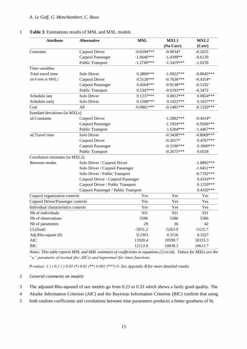
Table 3: Estimations results of MNL and MXL models 1

Attribute Alternative MNL MXL1 MXL2

(No Corr) (Corr)

Constants Carpool Driver -0.6594 *** -0.9034 * -0.2655

Carpool Passenger -1.0646 *** -1.4399 ** -0.6139

Public Transport -1.2749 *** -1.5419 *** -1.0259

Time variables

Total travel time

(in €/min in MNL)

Solo Driver 0.3806 *** -1.0922 *** -0.8645 ***

Carpool Driver 0.5126 *** -0.7636 *** -0.4354 *

Carpool Passenger 0.4564 *** -0.9138 *** -0.5192 ‘

Public Transport 0.5347 *** -0.6193 *** -0.3472

Schedule late Solo Driver 0.1237 *** 0.0812 *** 0.0824 ***

Schedule early Solo Driver 0.1568 *** 0.1422 *** 0.1637 ***

Cost All -0.0861 *** -0.1481 *** -0.1350 ***

Standard deviations (in MXLs)

sd Constants Carpool Driver -1.2882 *** -0.4414 *

Carpool Passenger -1.1924 *** -0.9266 ***

Public Transport 1.6304 *** -1.4467 ***

sd Travel time Solo Driver -0.3438 *** -0.8069 ***

Carpool Driver -0.3017 * 0.4767 ***

Carpool Passenger -0.3196 *** 0.3900 ***

Public Transport -0.2675 *** 0.0558

Correlation estimates (in MXL2)

Between modes Solo Driver / Carpool Driver -1.0892 ***

Solo Driver / Carpool Passenger -1.0451 ***

Solo Driver / Public Transport -0.7192 ***

Carpool Driver / Carpool Passenger 0.4316 ***

Carpool Driver / Public Transport 0.1259 ***

Carpool Passenger / Public Transport 0.4102 ***

Carpool organization controls Yes Yes Yes

Carpool Driver/Passenger controls Yes Yes Yes

Individual characteristics controls Yes Yes Yes

Nb of individuals 931 931 931

Nb of observations 5586 5586 5586

Nb of parameters 29 36 42

LL(final) -5931.2 -5263.9 -5125.7

Adj.Rho-square (0) 0.2303 0.3156 0.3327

AIC 11920.4 10599.7 10335.3

BIC 12112.6 10838.3 10613.7

Notes: This table reports MNL and MXL estimates of coefficients in equations (1) to (4). Values for MXLs are the

“µ” parameter of normal (for ASCs) and lognormal (for time) functions.

P-values: 1 ( ) 0.1 (‘) 0.05 (*) 0.01 (**) 0.001 (***) 0. See Appendix B for more detailed results

General comments on models 2

The adjusted Rho-squared of our models go from 0.23 to 0.33 which shows a fairly good quality. The 3

Akaike Information Criterion (AIC) and the Bayesian Information Criterion (BIC) confirm that using 4

both random coefficients and correlations between time parameters produces a better goodness of fit. 5


16

Constants 1

In MNL and MXL1, the alternative-specific constants (ASC) of all modes are significantly negative, 2

Solo Driver being the reference. It means that all other variables equaling zero, there is on average a 3

preference for Solo Driver mode over all the other modes. These preferences are high as the monetary 4

equivalent11 of the ASC in MNL go from 7.7€ (Carpool Driver) to 14.8€ (Public Transport). It means 5

that on average and other variables equaling 0, an individual in our sample (i.e. a current solo driver) is 6

willing to accept to switch to Public Transport if he receives at least 14.8€. The estimations of the ASC 7

standard deviations in MXL1 and MXL 2 also show that these preferences are largely distributed across 8

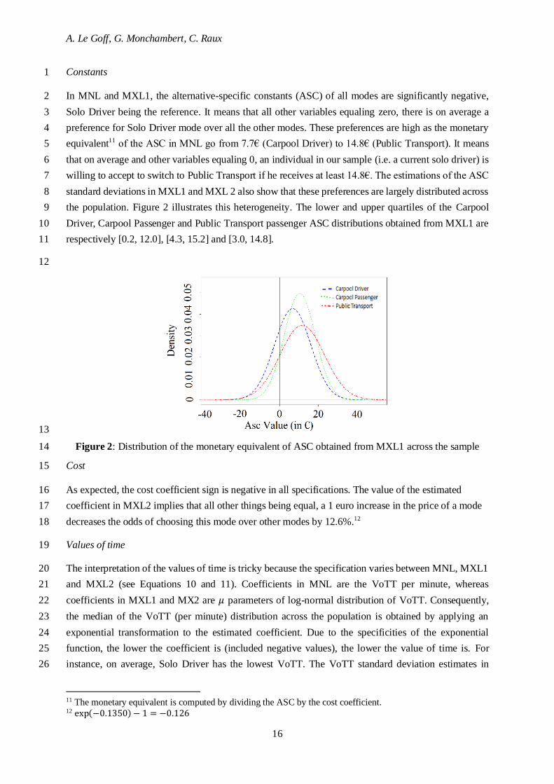
the population. Figure 2 illustrates this heterogeneity. The lower and upper quartiles of the Carpool 9

Driver, Carpool Passenger and Public Transport passenger ASC distributions obtained from MXL1 are 10

respectively [0.2, 12.0], [4.3, 15.2] and [3.0, 14.8]. 11

12

13

Figure 2: Distribution of the monetary equivalent of ASC obtained from MXL1 across the sample 14

Cost 15

As expected, the cost coefficient sign is negative in all specifications. The value of the estimated 16

coefficient in MXL2 implies that all other things being equal, a 1 euro increase in the price of a mode 17

decreases the odds of choosing this mode over other modes by 12.6%.12 18

Values of time 19

The interpretation of the values of time is tricky because the specification varies between MNL, MXL1 20

and MXL2 (see Equations 10 and 11). Coefficients in MNL are the VoTT per minute, whereas 21

coefficients in MXL1 and MX2 are 𝜇 parameters of log-normal distribution of VoTT. Consequently, 22

the median of the VoTT (per minute) distribution across the population is obtained by applying an 23

exponential transformation to the estimated coefficient. Due to the specificities of the exponential 24

function, the lower the coefficient is (included negative values), the lower the value of time is. For 25

instance, on average, Solo Driver has the lowest VoTT. The VoTT standard deviation estimates in 26

11 The monetary equivalent is computed by dividing the ASC by the cost coefficient. 12 exp(−0.1350) − 1 = −0.126


17

MXL1 and MXL2 are significant. This means that VoTTs are distributed across the population and 1

validates the assumption of heterogeneity. 2

The estimates of the 𝜇 parameters of log-normal distribution of carpool passenger and public transport 3

VoTT in MXL2 do not significantly differ from 0. However, the specification of these coefficients 4

described in Equation (11) suggests that the VoTT are driven by the correlation between travel time 5

parameters. We also observe that values of time are higher in MXL2 than in MXL1 (total travel time 6

estimates are higher for the four modes, see Table 3). Introducing correlation between modes VoTTs 7

reduces the impact of ASCs on preferences and by compensation increases the impact of VoTTs. Indeed, 8

the estimates of correlation coefficients are significantly different from 0. Their interpretation is as 9

follows: the coefficients comparing the Solo Driver mode and the others are negative, implying that 10

people who value higher the time spent as a solo driver will tend to value lower time spent in other 11

modes and vice versa. In contrast, the coefficients between the other modes are positively correlated, 12

which imply people having higher valuation of time spent in one of these modes (carpooling and public 13

transport) tends to value higher time in the other alternative modes to solo driving as well. We discuss 14

and illustrate these results in the following section. The introduction of these estimates also partly 15

explains why the Public Transport travel time parameter varies much less than others in MXL2 (see 16

Table 3), because heterogeneity of values of time in this mode is already correlated to other 17

heterogeneities in the three other modes. 18

Schedule delay 19

Schedule delay is presented only with solo driving mode in the survey. In all models, the cost of arriving 20

at destination one minute earlier than the preferred arrival time (0.16€/minute in MXL2) is found to be 21

higher than the cost of arriving one minute later (0.08€/minute in MXL2. This is an unexpected result 22

which will be discussed in the next section. Our results also suggest that the value of the schedule delay 23

early is around 40% of the VoTT value. 24

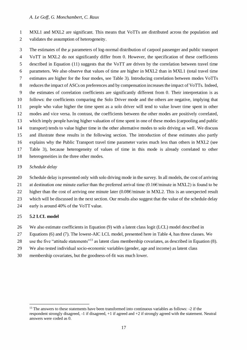
5.2 LCL model 25

We also estimate coefficients in Equation (9) with a latent class logit (LCL) model described in 26

Equations (6) and (7). The lowest-AIC LCL model, presented here in Table 4, has three classes. We 27

use the five “attitude statements”13 as latent class membership covariates, as described in Equation (8). 28

We also tested individual socio-economic variables (gender, age and income) as latent class 29

membership covariates, but the goodness-of-fit was much lower. 30

13 The answers to these statements have been transformed into continuous variables as follows: -2 if the

respondent strongly disagreed, -1 if disagreed, +1 if agreed and +2 if strongly agreed with the statement. Neutral

answers were coded as 0.


18

Table 4: Estimations results of LCL model 1

Attribute Alternative LCL

Class A Class B Class C

Constants Carpool Driver 0.4636** -3.6684*** -0.7033**

Carpool Passenger -1.0196** -3.1775* 0.3062

Public Transport -3.4962*** -6.6848*** 0.6728**

Time variables

Total travel time(in €/min) Solo Driver 0.2581*** 0.3223*** 0.5538***

Carpool Driver 0.3699*** 0.5046*** 0.6874***

Carpool Passenger 0.2264*** 0.6865* 0.6476***

Public Transport 0.2187* -0.0072 0.7023***

Schedule late Solo Driver -0.0394 -0.0533* 0.0595**

Schedule early Solo Driver 0.3172*** 0.1310*** 0.1593***

Cost -0.1097***

Latent Class Allocation Variables

Average Latent Class Allocation Probability 0.41 0.28 0.32

S1 (“car traffic major source”) 0 -0.1055 0.1165

S2 (“satisfied with my choices”) 0 0.3205*** -0.3498***

S3 (“could change easily”) 0 -0.4941*** 0.2437**

S4 (“opinion matter”) 0 -0.1899* -0.1622*

S5 (“personally responsible”) 0 -0.0541 -0.0544

Carpool organization controls Yes

Carpool Driver/Passenger controls Yes

Individual characteristics controls Yes

Nb of individuals 931

5586

55

-5027.3

0.3437

10164.7

10529.2

Nb of observations

Nb of parameters

LL(final)

Adj.Rho-square (0)

AIC

BIC

Notes: This table reports LCL estimates of coefficients in equations (1) to (4).

P-values: 1 ( ) 0.1 (‘) 0.05 (*) 0.01 (**) 0.001 (***) 0. See Appendix B for more detailed results

Latent class probability and covariates 2

The sample average probability of belonging to Class A is 41%, 28% for Class B and 32% for Class C. 3

We find that individuals who agree with the statements S2 (“I am satisfied with my daily trip choices”) 4

and disagree with statement S3 (“I can or could easily change the way I travel on a daily basis”) have a 5

higher probability of belonging to Class B. On the contrary, individuals who disagree with S2 and agree 6

with S3 are more likely to belong to Class C. Finally, individuals who agree with S4 (“The opinion of 7

people who matter to me is important for the way I travel on a daily basis”) are more likely to be in 8

Class A. 9

Mode preferences 10

Mode preferences are compared between classes taking into account VoTTs and ASCs. For instance 11

Class C has higher VoTT than other classes, but it is compensated by much lower ASC. On the contrary, 12

Class A has low VoTT but high ASC. Moreover, in class B Public Transport ASC is so high that even 13

if the VoTT estimate is not significant, the cost of this alternative will always be valued much higher 14


19

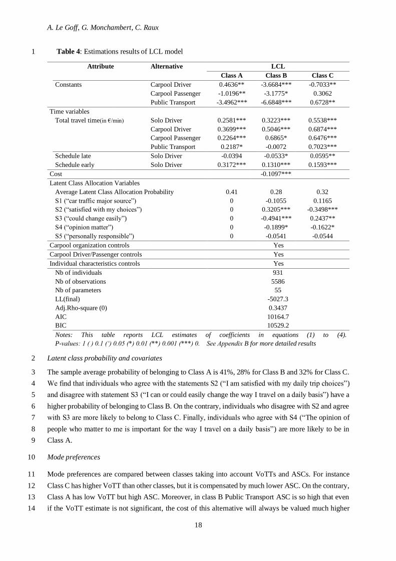
than the Solo Driver one. This is illustrated with the Table 5 below which displays generalized costs for 1

each class of the LCL model for a 40 minutes trip (average trip duration in the sample, see 2

Table 2). 3

Table 5 : Generalized costs for a 40-minute trip in each mode and class in LCL 4

5

Figure 3 shows a comparison of these generalized costs for the four modes in each class across the trip 6

duration. Class A has overall a lower generalized cost for Solo Driver than other classes. This class 7

values equally lower both Solo Driver and Carpool Driver, and higher Carpool Passenger and much 8

higher Public Transport. Class B values all the modes other than Solo Driver much higher than this one. 9

Finally, Class C presents very similar generalized costs for the four modes with a slightly higher value 10

for Carpool Driver. 11

Class A

Class B Class C

Notes: We take the values at the sample mean i.e. the representative individual14 making the representative trip to compute sample average values.

Figure 3: Generalized Costs of a trip for the representative individual depending on mode and travel time 12

14 The representative individual is defined with the mean values for each individual characteristic displayed in

Table 2

Class A Class B Class C

Solo Driver 10€ 13€ 22€

Carpool Driver 11€ 54 € 35€

Carpool Passenger 24€ 62€ 28€

Public Transport 40€ 60 € 22€


20

6. DISCUSSION 1

First the values of travel time are discussed, second the preferences stated by the individuals are 2

analyzed. Finally, we derive some policy implications. 3

Values of travel time 4

An important result is the stable ranking between modal alternatives through the models. Table 6 below 5

illustrate this ranking through relative values, 100 being the value of time in Solo Driver for each model. 6

Table 6: Relative Values of Time with Solo Driver as Reference 7

8

In the MNL and MXL models travel time by the four modes are valued from the lowest to the highest 9

as follows: Solo Driver, Carpool Passenger, Carpool Driver and Public Transport. These results suggest 10

time in Carpool Driver is valued around 40% higher than solo driving, Carpool Passenger around 20% 11

higher and Public Transport around 60% higher, based on MXL1 results. 12

As respondents are currently solo drivers, there is no surprise in finding Solo Driver VoTT as the lowest. 13

An interesting result in this ranking is that the Carpool Driver travel time is valued higher than Carpool 14

Passenger, even though our respondents are current drivers. This result shows that the longer the travel, 15

the more the Carpool Passenger alternative is likely to be chosen compared to the Carpool Driver one. 16

This could be explained by several facts: driving can be stressful, the time spent as a passenger can be 17

used in a different and more pleasant way than the time spent as a driver (reading or consulting one's 18

smartphone for instance). 19

Values of time found in this survey are higher than what Wardman et al. (2016) and Shires & De Jong 20

(2009) found for commuting by car in France, respectively 11.8€2019/h and 15.4€2019/h. Several reasons 21

may explain this. First, our sample is composed only of currently solo drivers, who may have higher 22

incomes than the whole population and hence higher values of time. Another explanation could be that 23

the values we find can be considered from a willingness to accept (WTA) perspective since the exercises 24

challenge whatsolo drivers are willing to accept to switch to another mode (see also Monchambert, 25

2020). In the VoTT field, De Borger and Forsgerau (2008) found an important gap between WTP and 26

WTA with a 1 to 4 factor. 27

Attribute Alternative MNL MXL1

(No Corr)

MXL2

(Corr)

TT Solo Driver

100

(22.8€/h)

100

(20.1€/h*)

100

(25.3€/h*)

Carpool Driver 135 139 153

Carpool Passenger 120 120 141

Public Transport 141 161 167

Notes: For each model, 100 represent the value of 1 hour spent in the Solo Driver mode

* Values for MXL are the median values of the estimated lognormal distribution


21

The schedule late delay is valued lower than schedule early delay. This result is unexpected and opposite 1

to what is found in the literature (de Palma & Fontan, 2000). It could be explained because respondents 2

may have misunderstood schedule delay. They could have only observed that their departure time was 3

later than usual and hence thought their total travel time was lower, thinking all the alternatives were 4

arriving on time. We can also assume respondents may have a lot of flexibility, no time constraints they 5

cannot override. However, the scheduled early value is found around 40% of the Solo Driver VoTT. 6

This result is consistent with what was found in de Palma & Fontan (2000) in Paris, around 35%. 7

Other perspectives on the heterogeneity of preferences 8

Figure 4 below combines results from MXL2 and LCL models. Each individual is represented by a point 9

showing its VoTT, estimated with the MXL2 model. Each point is characterized by the latent class to 10

which the individual is most likely to belong in LCL. A black line of slope 1 representing points with 11

equal VoTTs is added. 12

It can be observed that these points are organized in an increasing way. This means that the larger the 13

VoTT is for the Solo Driver mode, the larger it is for the other modes as well. One can also see that the 14

points associated with class C are distributed in a rather heterogeneous way, some with values of time 15

among the lowest and others among the highest. Points associated with the two other classes are more 16

homogeneous with lower values for class A and higher for class B. 17

Furthermore, notice that some points are clearly distinguishable from the others on the right part of the 18

plots. They are associated with class B and far below the black line. This means these individuals 19

therefore tend to value very high every other mode and value proportionally lower the Solo Driver. This 20

result is consistent with what was found in the MXL correlation estimates. Individuals associated with 21

Class C are in the upper part of scatterplots in the graphs which compare Solo Driver and passenger 22

modes VoTT. This means these individuals have the lowest VoTT for passenger modes proportionally 23

to their Solo Driver VoTT. Similarly, the points associated with class A can be found in the upper part 24

of the scatterplot on graph comparing Solo Driver VoTT and Carpool Driver VoTT and hence they value 25

the Carpool Driver proportionally lower. 26


22

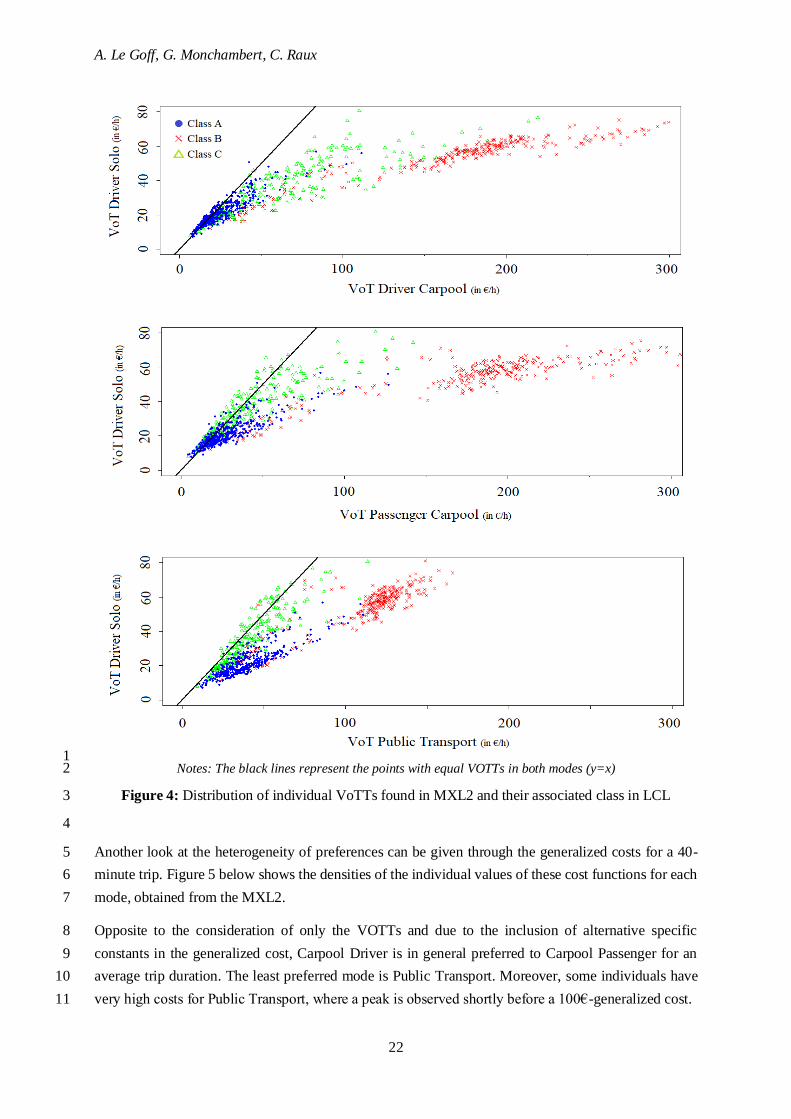
1 Notes: The black lines represent the points with equal VOTTs in both modes (y=x) 2

Figure 4: Distribution of individual VoTTs found in MXL2 and their associated class in LCL 3

4

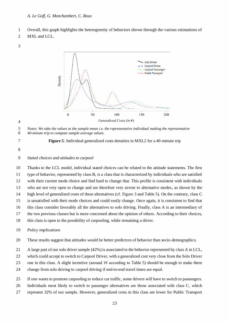
Another look at the heterogeneity of preferences can be given through the generalized costs for a 40-5

minute trip. Figure 5 below shows the densities of the individual values of these cost functions for each 6

mode, obtained from the MXL2. 7

Opposite to the consideration of only the VOTTs and due to the inclusion of alternative specific 8

constants in the generalized cost, Carpool Driver is in general preferred to Carpool Passenger for an 9

average trip duration. The least preferred mode is Public Transport. Moreover, some individuals have 10

very high costs for Public Transport, where a peak is observed shortly before a 100€-generalized cost. 11


23

Overall, this graph highlights the heterogeneity of behaviors shown through the various estimations of 1

MXL and LCL. 2

3

4

Notes: We take the values at the sample mean i.e. the representative individual making the representative 5 40-minute trip to compute sample average values. 6

Figure 5: Individual generalized costs densities in MXL2 for a 40-minute trip 7

8

Stated choices and attitudes to carpool 9

Thanks to the LCL model, individual stated choices can be related to the attitude statements. The first 10

type of behavior, represented by class B, is a class that is characterized by individuals who are satisfied 11

with their current mode choice and find hard to change that. This profile is consistent with individuals 12

who are not very open to change and are therefore very averse to alternative modes, as shown by the 13

high level of generalized costs of these alternatives (cf. Figure 3 and Table 5). On the contrary, class C 14

is unsatisfied with their mode choices and could easily change. Once again, it is consistent to find that 15

this class consider favorably all the alternatives to solo driving. Finally, class A is an intermediary of 16

the two previous classes but is more concerned about the opinion of others. According to their choices, 17

this class is open to the possibility of carpooling, while remaining a driver. 18

Policy implications 19

These results suggest that attitudes would be better predictors of behavior than socio-demographics. 20

A large part of our solo driver sample (42%) is associated to the behavior represented by class A in LCL, 21

which could accept to switch to Carpool Driver, with a generalized cost very close from the Solo Driver 22

one in this class. A slight incentive (around 1€ according to Table 5) should be enough to make them 23

change from solo driving to carpool driving if end-to-end travel times are equal. 24

If one wants to promote carpooling to reduce car traffic, some drivers will have to switch to passengers. 25

Individuals most likely to switch to passenger alternatives are those associated with class C, which 26

represent 32% of our sample. However, generalized costs in this class are lower for Public Transport 27


24

than for Carpool Passenger. As a result, Public Transport is likely to be the preferred shift mode of solo 1

drivers in class C in the case that the introduction of a HOV lane increases the generalized cost of Solo 2

Driver. Having more former solo drivers in public transport would indeed decrease the share of solo 3

driving but this would also make more difficult the setting-up of carpool parties. There is a risk of 4

scarcity of carpool passengers, who are the limiting resource in carpool matching. Specific incentives 5

should be designed to ease the recruitment of carpool passengers. 6

Finally, there are some people for whom it will be complicated, if not impossible, to change their minds. 7

Fortunately, these people who are resistant to change represent only 28% of our sample. 8

7. CONCLUSION 9

This paper has estimated values of travel time of four modes (Solo Driver, Carpool Driver, Carpool 10

Passenger and Public Transport) for commuting trips. A stated choice survey conducted on a 11

931-respondent sample allowed us to understand modal choices through two different types of models 12

allowing for heterogeneous tastes: mixed multinomial and latent class logits. 13

The originality of this paper is the focus on carpool specific values of time for daily trips, both as a 14

driver and as a passenger. A comparison of these values is also provided with VoTT by more classic 15

modes found in the literature: solo driving and public transport. It gives us a ranking of mode-specific 16

values of time for currently solo-driving commuters, which is from the lowest to the highest: Solo 17

Driver, Carpool Passenger (around 20% higher than Solo Driver), Carpool Driver (around 40% higher) 18

and Public Transport (around 60% higher). 19

Individuals also react heterogeneously in their mode choice behavior. The latent-class analysis reveals 20

these heterogeneities are explained better by the attitude statements than by socio-economic variables. 21

Besides, it shows that finding carpool drivers seems easier than finding carpool passengers due to the 22

competition from public transport for individuals who agree to become passengers. Incentives will 23

therefore have to be adapted to the population to convince car commuters to switch to carpooling, 24

especially as a passenger, which should be the scarce resource. 25

Finally, we know carpool organization and individual variables may impact carpool choices. This raises 26

the question of how impactful matching between individuals can be on the decision to carpool or not. 27

Besides, the different stages that compose end-to-end travel time can be valued differently, such as 28

access to carpool meeting or waiting times. These effects on commuting mode choice need to be 29

explored through further research. 30

31

Aknowledgements 32

This research was funded by the Auvergne-Rhône-Alpes region (Pack ambition recherche 2018: Projet 33

Covoit’AURA). The authors acknowledge the support of IRT SystemX and the partners of the Lyon 34

Carpooling Experimentation project (LCE): Métropole de Lyon, Vinci Autoroutes, APRR, Ecov who 35


25

participated in the dissemination of the survey. We also thank the participants in of the ITEA 2019 1

conference in Paris and ERSA 2019 conference in Lyon for their valuable comments. 2

3

REFERENCES 4

AASHTO (2013) Commuting in America 2013. The National Report on Commuting Patterns and 5

Trends. Brief 10. Commuting Mode Choice. 32 p. 6

ADEME-INDDIGO, S. A. S. (2015). Leviers d’actions pour favoriser le covoiturage de courte distance, 7

évaluation de l’impact sur les polluants atmosphériques et le CO2. Leviers d’actions, benchmark 8

et exploitation de l’enquête nationale Transports et déplacements (ENTD), Rapport final, Paris, 9

ADEME. 10

Ajzen, I. (1991). The theory of planned behavior. Organizational behavior and human decision 11

processes, 50(2), 179-211. Blayac, T., & Adjeroud, F. (2018). Perception du temps de transport 12

par les usagers de l’autocar et du covoiturage: quelle valeur du temps pour les déplacements 13

longue distance en France (No. hal-02099824). 14

Chan, N. D., & Shaheen, S. A. (2012). Ridesharing in North America: Past, present, and 15

future. Transport reviews, 32(1), 93-112. 16

Chaube, V., Kavanaugh, A. L., & Perez-Quinones, M. A. Leveraging social networks to embed trust in 17

rideshare programs. In 2010 43rd Hawaii International Conference on System Sciences, 2010. 18

1-8. IEEE. 19

ChoiceMetrics Ngene 1.1.1 User Manuel & Reference Guide, Australia, 2012. 20

Daganzo, C. F., & Cassidy, M. J. (2008). Effects of high occupancy vehicle lanes on freeway 21

congestion. Transportation Research Part B: Methodological, 42(10), 861-872. 22

Daly, A., Hess, S. & Train, K. (2012) Assuring finite moments for willingness to pay in random 23

coefficient models. Transportation 39, 19 – 31 24

De Borger, B., & Fosgerau, M. (2008). The trade-off between money and travel time: A test of the 25

theory of reference-dependent preferences. Journal of urban economics, 64(1), 101-115. 26

de Palma, A. Fontan, C. (2000). Enquête MADDIF. http://temis.documentation.developpement-27

durable.gouv.fr/docs/Temis/0072/Temis-0072657/RMT00-040.pdf Acessed Feb. 2019 28

ENTD, 2008. Enquête nationale transport et déplacements. 29

Furuhata, M., Dessouky, M., Ordóñez, F., Brunet, M. E., Wang, X., & Koenig, S. Ridesharing: The 30

state-of-the-art and future directions. Transportation Research Part B: Methodological, 2013. 31

57: 28-46. 32

Greene, W.H., Hensher, D.A., (2003) A latent class model for discrete choice analysis: contrasts with 33

mixed logit Transportation research Part B 37, 681 – 698 34

Hensher, D. A., Rose, J. M., & Greene, W. H. Applied choice analysis. Second Edition. Cambridge 35

University Press, 2015. 36

Hess, S., Bierlaire, M., & Polak, J. W. (2005). Estimation of value of travel-time savings using mixed 37

logit models. Transportation Research Part A: Policy and Practice, 39(2-3), 221-236. 38

http://temis.documentation.developpement-durable.gouv.fr/docs/Temis/0072/Temis-0072657/RMT00-040.pdf%20Acessed%20Feb.%202019

http://temis.documentation.developpement-durable.gouv.fr/docs/Temis/0072/Temis-0072657/RMT00-040.pdf%20Acessed%20Feb.%202019


26

Hess, S. & Rose, J. M. (2009). Allowing for intra-respondent variations in coefficients estimated on 1

repeated choice data. Transportation Research Part B: Methodological, 43(6), 708-719. 2

Hess, S., Rose, J.M. & Polak, J.W. (2010) Non-Trading, lexicographic and inconsistent behaviour in 3

stated choice data. Transportation research Part D, 15, 405 – 417 4

Hess, S. & Palma, D. Apollo: a flexible, powerful and customisable freeware package for choice model 5

estimation and application, Journal of Choice Modelling, 2019. 6

Hess, S. & Palma, D. Apollo version 0.1.0, user manual, www.ApolloChoiceModelling.com, 2020. 7

INRIX. Global Traffic Scorecard, 2019. 8

Jara-Díaz, S. R., Munizaga, M. A., Greeven, P., Guerra, R., & Axhausen, K. (2008). Estimating the 9

value of leisure from a time allocation model. Transportation Research Part B: 10

Methodological, 42(10), 946-957. 11

Li, J., Embry, P., Mattingly, S. P., Sadabadi, K. F., Rasmidatta, I., & Burris, M. W. (2007). Who chooses 12

to carpool and why? Examination of Texas carpoolers. Transportation Research 13

Record, 2021(1), 110-117. 14

Louviere, J. J., Hensher, D. A., & Swait, J. D. Stated choice methods: analysis and applications. 15

Cambridge university press, 2000. 16

McFadden, D. and Train, K. (2000) Mixed MNL models for discrete response. Journal of Applied 17

Econometrics 15: 447-470. 18

Monchambert, G. (2020). Why do (or don’t) people carpool for long distance trips? A discrete choice 19

experiment in France. Transportation Research Part A: Policy and Practice, 132, 911-931. 20

Quinet, E. L’évaluation socio-économique en période de transition. Valeurs du temps. 2013. 21

https://www.strategie.gouv.fr/sites/strategie.gouv.fr/files/archives/Valeur-du-temps.pdf 22

Accessed Feb. 2019. 23

Rose, J. M., Bliemer, M. C., Hensher, D. A., & Collins, A. T. (2008). Designing efficient stated choice 24

experiments in the presence of reference alternatives. Transportation Research Part B: 25

Methodological, 42(4), 395-406.Schijns, S., & Eng, P. (2006). High occupancy vehicle lanes–26

worldwide lessons for European practitioners. WIT Transactions on the Built Environment, 89. 27

Schwartz, S. H. (1977). Normative influences on altruism. Advances in experimental social 28

psychology, 10(1), 221-279.. 29

Shaheen, S., Stocker, A. & Mundler, M. (2017) Online and app-based carpooling in France: Analyzing 30

users and practices - A study of BlaBlaCar. Disrupting Mobility, 181 – 196 31

Shen, J., Sakata, Y., Hashimoto, Y., (2006) Discussion Papers In Economics And Business. A 32

Comparison between Latent Class Model and Mixed Logit Model for Transport Mode Choice: 33

Evidences from Two Datasets of Japan. 20. 34

Shires, J. D., & De Jong, G. C. (2009). An international meta-analysis of values of travel time 35

savings. Evaluation and program planning, 32(4), 315-325. 36

Shoup, D. C. (1997). Evaluating the effects of cashing out employer-paid parking: eight case 37

studies. Transport Policy, 4(4), 201-216. 38

Small, K. A. (2012). Valuation of travel time. Economics of transportation, 1(1-2), 2-14. 39

Train, K. E. (2009). Discrete choice methods with simulation. Second Edition. Cambridge university 40

press. 41


27

Train, K., Weeks, M. (2005) Discrete choice models in preference space and willingness-to-pay space. 1

In: Application of Simulation Methods in Environmental and Resource Economics, chap. 1, 1 2

– 16 3

Ugolik, W., O'Connell, N., Gluck, J. S., & Sookram, A. (1996). Evaluation of high-occupancy-vehicle 4

lanes on Long Island Expressway. Transportation research record, 1554(1), 110-120. 5

Wall, R., Devine-Wright, P., & Mill, G. A. (2007). Comparing and combining theories to explain 6

proenvironmental intentions: The case of commuting-mode choice. Environment and 7

behavior, 39(6), 731-753. 8

Wardman, M., Chintakayala, P., de Jong, G., & Ferrer, D. (2012). European wide meta-analysis of 9

values of travel time. 10

Wardman, M., Chintakayala, V. P. K., & de Jong, G. (2016). Values of travel time in Europe: Review 11

and meta-analysis. Transportation Research Part A: Policy and Practice, 94, 93-111. 12

13


28

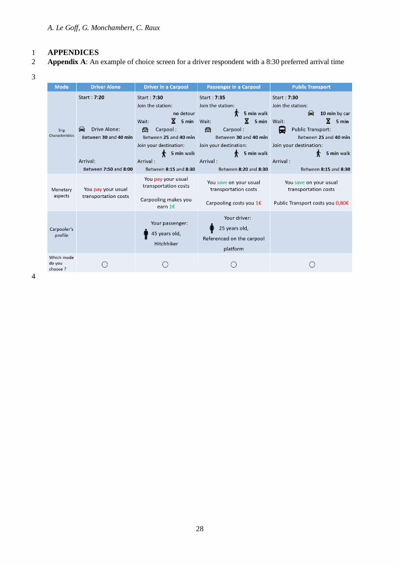
APPENDICES 1

Appendix A: An example of choice screen for a driver respondent with a 8:30 preferred arrival time 2

3

4


29

Appendix B: Results with Individual Parameters & Carpool Organization Controls 1

Attribute Alternative MNL MXL1 MXL2 LCL

(No Corr) (Corr) Class A Class B Class C

Constants Carpool Driver -0.6594 *** -0.9034 * -0.2655 0.4636** -3.6684*** -0.7033**

Carpool Passenger -1.0646 *** -1.4399 ** -0.6139 -1.0196** -3.1775* 0.3062

Public Transport -1.2749 *** -1.5419 *** -1.0259 -3.4962*** -6.6848*** 0.6728**

Time variables

Total travel time Solo Driver 0.3806 *** -1.0922 *** -0.8645 *** 0.2581*** 0.3223*** 0.5538***

Carpool Driver 0.5126 *** -0.7636 *** -0.4354 * 0.3699*** 0.5046*** 0.6874***

Carpool Passenger 0.4564 *** -0.9138 *** -0.5192 ‘ 0.2264*** 0.6865* 0.6476***

Public Transport 0.5347 *** -0.6193 *** -0.3472 0.2187* -0.0072 0.7023***

Schedule late Solo Driver 0.1237 *** 0.0812 *** 0.0824 *** -0.0394 -0.0533* 0.0595**

Schedule early Solo Driver 0.1568 *** 0.1422 *** 0.1637 *** 0.3172*** 0.1310*** 0.1593***

Cost All -0.0861 *** -0.1481 *** -0.1350 *** -0.1097***

Standard deviations (in MXLs)

sd Constants Carpool Driver -1.2882 *** -0.4414 *

Carpool Passenger -1.1924 *** -0.9266 ***

Public Transport 1.6304 *** -1.4467 ***

sd Travel time Solo Driver -0.3438 *** -0.8069 ***

Carpool Driver -0.3017 * 0.4767 ***

Carpool Passenger -0.3196 *** 0.3900 ***

Public Transport -0.2675 *** 0.0558

Correlation estimates (in MXL2)

Between modes Solo Driver / Carpool Driver -1.0892 ***

Solo Driver / Carpool Passenger -1.0451 ***

Solo Driver / Public Transport -0.7192 ***

Carpool Driver / Carpool Passenger 0.4316 ***

Carpool Driver / Public Transport 0.1259 ***

Carpool Passenger / Public Transport 0.4102 ***

Latent Class Allocation Variables

Average Latent Class Allocation Probability 0.41 0.28 0.32

S1 (“car traffic major source”) 0 -0.1055 0.1165

S2 (“satisfied with my choices”) 0 0.3205 *** -0.3498***

S3 (“could change easily”) 0 -0.4941*** 0.2437**

S4 (“opinion matter”) 0 -0.1899* -0.1622*

S5 (“personally responsible”) 0 -0.0541 -0.0544

Gender

(1 = male)

Carpool Driver -0,193** -0,335* -0,16 0,008

Carpool Passenger -0,274** -0,371* -0,23 0,005

Public Transport -0,185 ‘ -0,379 ‘ -0,265 0,164

Age

(1 = 46yo

or more)

Carpool Driver -0,415*** -0,672*** -0,413** -0,247*

Pass Cp -0,43*** -0,591*** -0,368 ‘ -0,143

Pub T 0,01 -0,098 0,127 0,39**

Income

Driv Cp 0,148*** 0,195* 0,169 ‘ 0,085 ‘

Pass Cp 0,041 0,013 -0,044 -0,113 ‘

Pub T 0,119* 0,151 0,009 -0,115

Male Passenger Driv Cp -0,242*** -0,365*** -0,35*** -0,317***

Age Passenger Driv Cp 0,032 0,13 0,108 0,08

Male Driver Pass Cp -0,162 -0,274 ‘ -0,292* -0,219*

Age Driver Pass Cp 0,037 0,072 0,083 0,039


30

1

2

3

Appendix C: Non-traders & Fast answerers in the sample

Caracteristics Answered in < 6 sec Answered in > 6 sec Total

Never Choose

Solo Driver 60 625 685

Choose Solo Driver

at least once 220 931 1151

Total 280 1556 1836

4

Carpool Organization

Relative Driv Cp 0 (ref) 0 (ref) 0 (ref) 0 (ref)

Planif Platform -0,141 -0,24 ‘ -0,176 -0,204

Spont Platform 0,15 0,224 0,181 0,139

Hitchhiker -0,12 -0,211 -0,256 -0,245 ‘

Relative Pass Cp 0 (ref) 0 (ref) 0 (ref) 0 (ref)

Planif Platform -0,14 -0,263 -0,279 -0,277 ‘

Spont Platform 0,103 0,121 0,017 0,025

Hitchhiker -0,37* -0,542* -0,566 ‘ -0,453**

Carpool organization controls Yes Yes Yes Yes

Carpool Driver/Passenger controls Yes Yes Yes Yes

Individual characteristics controls Yes Yes Yes Yes

Nb of individuals 931 931 931 931

Nb of observations 5586 5586 5586 5586

Nb of parameters 29 36 42 55

LL(final) -5931.2 -5263.9 -5125.7 -5027.3

Adj.Rho-square (0) 0.2303 0.3156 0.3327 0.3437

AIC 11920.4 10599.7 10335.3 10164.7

BIC 12112.6 10838.3 10613.7 10529.2

P-values: 1 ( ) 0.1 (‘) 0.05 (*) 0.01 (**) 0.001 (***) 0.


31

Appendix D: Trip attributes and levels in stated choice design 1

Attributes Alternatives Levels

Time variables

Schedule early/late Solo Driver 0, 30, 60 minutes (earlier or later)

Access time Passenger modes* 5 minutes walking (ref), 10 minutes by car, 20 minutes

by car

Detour time Carpool Driver 0, 5, 10 minutes

Waiting time Passenger modes and

Driver in Spontaneous Carpool 0, 5, 10 minutes

In vehicle travel time All Solo Driver: (0.8, 1.1, 1.5) * usual_tt Other modes:

(0.6, 0.9, 1.2) *usual_tt

Travel time variability All (0.1, 0.3, 0.5) * TT

Egress time Passenger modes

Carpool passenger: 5 min walking (ref), 10/20 min by

Public Transport

Public transport: 5 min walking

Cost (in €) Carpool modes* and Public

Transport

Carpool Driver: receives (0, 0.02, 0.05, 0.1) * usual_tt

Carpool Passenger: pays (0, 0.02, 0.05, 0.1) * usual_tt

Public transport: pays 0.8

Carpooler profile

Carpooler matching Carpool modes Planned, Spontaneous

Carpooler Gender Male, Female


Carpooler Age 25, 45, 65 years old


Notes: Passenger modes: Carpool Passenger and Public Transport. Carpool modes: Carpool Driver and

Carpool Passenger. “usual_tt” is the usual travel time the respondent reports in the survey

2

values of time for carpool commuting with hov lanes: a

Documents