validation of supersonic film cooling modeling for … · a flat plate 32.28 inchesin length. ......
TRANSCRIPT

Validation of Supersonic Film Cooling Modeling for Liquid Rocket Nozzle Applications
Christopher I. Morris and Joseph H. Ruf
NASA/George C. Marshall Space Flight CenterER42/Fluid Dynamics Branch
Marshall Space Flight Center, AL 35812
ABSTRACT
Submitted to The 46th AIAA/ASME/SAE/ASEE Joint Propulsion Conference & Exhibit
Film cooling is used to protect walls in several aerospace applications, such as turbine blades, combustors, and rocket nozzles. In the latter application, the freestream flow, and often the film itself, are supersonic. Supersonic Film Cooling (SSFC) has been used in several liquid rocket engine designs, such as the F-1, LE-5A, LE-5B and, now under development, the J-2X. Due to the comparatively large film-cooled nozzle extension on the J-2X design, there is a critical need to assess the accuracy of CFD models in representative SSFC flowfields.
In this paper, a CFD analysis is reported for several Helium and Hydrogen SSFC experimentsdescribed in Refs. 1-4. These experiments were performed during the NASP program in the late 1980s and early 1990s. The experiments employed a reflected shock tunnel to generate the Mach 6.4 freestream flow. The approach boundary layer for the freestream flow developed over a flat plate 32.28 inches in length. The coolant flow was provided by an array of 40 2-D coolant nozzles, each 0.12 inches in height, and 0.404 inches in width at the exit plane. Mixing of the coolant and freestream flows occurred over another 17 inches of flat plate. The Helium coolant cases (Refs. 1-3) were designed to be velocity-matched with the freestream flow, while the Hydrogen coolant cases (Ref. 4) had substantial shear with the freestream. These experiments have previously been modeled in Refs. 5-6. All analysis in this work was performed using the Loci-CHEM CFD code, version 3.2-beta-10 (Ref 7). Loci-CHEM is a robust, parallelizable, multi-species viscous flow solver with the capability of using several different RANS turbulence models (Menter’s SST and BSL, Wilcox’s k-ω, and a realizable k-ε). Additionally, a hybrid RANS-LES mode is available for the SST, BSL and k-ω models.
Initially, a number of parametric studies were performed examining the influence of turbulence model, turbulence model compressibility correction, and turbulent Schmidt numbers on the results. These studies were carried out on a 2-D version of the grid, employing a coolant inflow profile specified at the injection plane, and extracted from the center of a separate 3-D nozzle simulation (a strategy suggested by Ref. 6). The studies found that all of these parameters can have a significant effect on the results.
Additionally, full 3-D simulations of the experiments have been conducted. In these cases, the computational domain comprises a single coolant nozzle in width, and employs periodic boundary conditions to simulate the large array of nozzles in the actual experiments. An example of a full 3-D calculation using the SST turbulence model for case 45 of Ref. 3 is shown
https://ntrs.nasa.gov/search.jsp?R=20100033432 2018-07-29T04:40:47+00:00Z

in Figure 1. The colormap depicts surface heat flux contours downstream of the coolant injection plane. As expected, the heat flux generally increases downstream of the coolant injection plane. However, the 3-D results also show that there is significant variation in the heat flux spanwise across each coolant nozzle width. These results are compared with the experimental data of Ref. 3 in Figure 2. While the model appears to capture the adiabatic cooling length reasonably well, it is evident that the SST turbulence model predicts significantly faster mixing than occurs in the experiment. Better agreement with experimental data has been obtained for the Hydrogen coolant cases of Ref. 4, possibly due to the considerable coolant-freestream shear present in those cases.
As none of the RANS models have yielded a consistently good model of the experimental heat flux data for all test cases, additional studies have been conducted to determine whether a time-averaged hybrid RANS-LES model will yield better agreement. These results will be reported in the final paper.
REFERENCES
1. Holden, M. S., Nowak, R. J., Olsen, G. C. and Rodriguez, K. M., “Experimental Studies of Shock Wave/Wall Jet Interaction in Hypersonic Flow”, AIAA Paper No. 90-0607, 1990.
2. Olsen, G. C., Nowak, R. J., Holden, M. S. and Baker, N. R., “Experimental Results for Film Cooling in 2-D Supersonic Flow Including Coolant Delivery Pressure, Geometry, and Incident Shock Effects”, AIAA Paper No. 90-0605, 1990.
3. Holden, M. S. and Rodriguez, K. M., “Experimental Studies of Shock-Wave/Wall-Jet Interaction in Hypersonic Flow,” NASA CR 195197, May 1994. See also NASA CR 195844, May 1994.
4. Olsen, G. C. and Nowak, R. J., “Hydrogen Film Cooling With Incident and Swept-Shock Interactions in a Mach 6.4 Nitrogen Free Stream”, NASA TM 4603, June 1995
5. Chamberlain, R., “Computation of Film Cooling Characteristics in Hypersonic Flow,” AIAA Paper No. 92-0657, 1992.
6. Chen, Y. S., Chen, C. P. and Wei, H., “Numerical Analysis of Hypersonic Turbulent Film Cooling Flows,” AIAA Paper No. 92-2767, 1992.
7. Luke, E. A., Tong, X., Wu, J., Tang, L. and Cinnella, P., “A Step Towards 'Shape-Shifting' Algorithms: Reacting Flow Simulations Using Generalized Grids,” AIAA Paper No. 2001-0897, 2001.
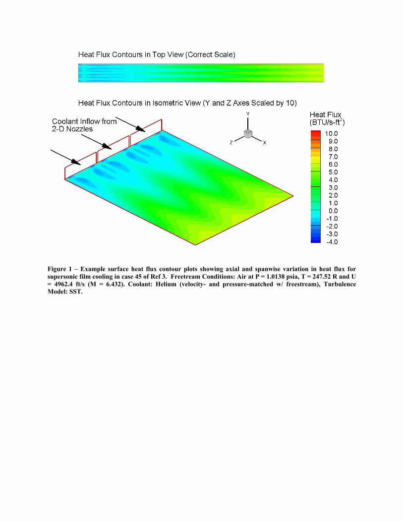
Figure 1 – Example surface heat flux contour plots showing axial and spanwise variation in heat flux for supersonic film cooling in case 45 of Ref 3. Freetream Conditions: Air at P = 1.0138 psia, T = 247.52 R and U = 4962.4 ft/s (M = 6.432). Coolant: Helium (velocity- and pressure-matched w/ freestream), Turbulence Model: SST.

Figure 2 – Comparison of CFD and experimental surface heat flux results for supersonic film cooling in case 45 of Ref 3. 2-D CFD simulation uses a coolant inflow profile extracted from a separate 3-D nozzle simulation. 3-D heat flux results are extracted from the nozzle centerline. Freetream Conditions: Air at P = 1.0138 psia, T = 247.52 R and U = 4962.4 ft/s (M = 6.432). Coolant: Helium (velocity- and pressure-matched w/ freestream), Turbulence Model: SST.
Validation of Supersonic Film Cooling Modeling for
Liquid Rocket Nozzle Applications
C. I. Morris∗ and J. H. Ruf∗
NASA Marshall Space Flight Center, Huntsville, AL, 35812, USA
Supersonic film cooling (SSFC) of nozzles has been used in several liquid rocket enginedesigns, and is being applied to the nozzle extension of the J-2X upper stage engine nowunder development. Due to the large size and challenging thermal load of the nozzleextension, there was a critical need to assess the accuracy of CFD models in representativeSSFC flowfields. This paper reports results from a CFD analysis of SSFC experimentsperformed at Calspan in the late 1980s and early 1990s. 2-D and 3-D CFD simulations of flatplate heating, coolant nozzle flow, and film cooling flowfields are discussed and comparedwith the experimental data. For the film cooling cases studied, the 3-D simulations predictthe initial mixing of the coolant and freestream in the adiabatic cooling region reasonablywell. However, the CFD simulations generally predict faster mixing in the developed flowregion of the flowfield than indicated by the experimental data. Hence, from an engineeringperspective, the CFD tool and modeling assumptions used are conservative.
Nomenclature
m mass flow rateq heat fluxa sound speedd deflectionI synthetic schlieren image intensityk specific turbulence kinetic energyM Mach number, U/ap pressures slot heightT temperatureU velocityx axial distance along test article, x = 0 at the coolant injection planey vertical distance from test article, y = 0 on the flat plate downstream of the coolant injection planey+ distance from wall in inner-law variables,
√ρwτwy/µw
z spanwise distance across test article, z = 0 on the centerline axis of symmetry of a coolant nozzle
Subscripts
0 stagnation∞ freestreamaw adiabatic wallc coolantt turbulentw wall
Symbols
δ99 boundary layer thickness (99% velocity)
∗Aerospace Engineer, Fluid Dynamics Branch/ER42, Senior Member AIAA.
1 of 21
American Institute of Aeronautics and Astronautics

ε specific turbulence dissipationµ viscosityω specific turbulence dissipation rateρ densityτ shear stressε scaling factor in deflection equation
I. Introduction
Film cooling is used to protect structures in several aerospace applications, such as gas turbine blades,rocket and scramjet combustors, and rocket nozzles. In scramjet combustors and rocket nozzles, the
freestream flow, and often the film itself, are supersonic. Supersonic film cooling (SSFC) of nozzles has beenused in several liquid rocket engine designs, such as Vulcain, LE-5A, LE-5B and, now under development,theJ-2X. The J-2X engine is an upper stage engine with a large area ratio nozzle. The nozzle consists of twosections: a regeneratively cooled section and a radiatively cooled section called the nozzle extension (NE).Between the two sections, the turbine exhaust gas is injected as a film barrier to reduce the heat load to theNE.
SSFC has been studied since the 1960s, with early research being primarily experimental. The pioneeringstudy of Goldstein et al.,1 at the University of Minnesota, investigated air and helium as coolants with aMach 3 air freestream. Parthasarathy and Zakkay,2 at New York University, investigated several coolantgases: air, helium, hydrogen and argon injected into a Mach 6 freestream. Further work at that facility, byZakkay et al.,3 investigated the effect of an adverse pressure gradient on SSFC effectiveness.
In the late 1980s and 1990s, several experimental studies were conducted examining SSFC. An inves-tigation of film cooling on a tetracone test article in a Mach 8 freestream was reported by Majeski andWeatherford4 of McDonnell Douglas. A study using nitrogen and hydrogen coolants in a Mach 3 freestreamwas conducted by Bass et al.5 at United Technologies Research Center. Studies using helium coolant in aMach 6.4 air freestream at Calspan were reported by Holden et al.6 and Olsen et al.7 A more detailed reportof this effort was provided by Holden and Rodriguez in Ref. 8. A later study using the same Calspan testarticle and facility, with both hydrogen and helium coolants, was reported by Olsen and Nowak.9 Air andhelium coolants, in a Mach 2.4 freestream, were studied in experimental works by Juhany and Hunt10 andJuhany et al.11 at Caltech. The effect of shock impingement on film cooling, of particular importance tothe scramjet engine application, was investigated in the Calspan and Caltech efforts. It was also a key focusof the experimental studies, using argon coolant in a Mach 2.35 nitrogen freestream, of Kanda et al.12 andKanda and Ono13 at National Aerospace Laboratory in Japan. A combined experimental and numericalstudy, using a mixture of cooled nitrogen and air as coolant in a Mach 2.78 air freestream, was conductedby Aupoix et al.14 at ONERA in France, with a view toward validating analysis tools for nozzle cooling inthe Vulcain engine.
Several efforts to numerically model these experiments with CFD have been reported. Chamberlain15 andChen et al.16 simulated the helium coolant Calspan experiments (Refs. 6–8). O’Connor and Haji-Sheikh17
simulated the earlier work of Ref. 1. Several recent studies have also investigated SSFC from a numericalmodeling standpoint. Takita and Musuya18 numerically investigated shock wave and combustion effects onSSFC using hydrogen. Peng and Jiang19 have also studied shock waves effects on film cooling, using nitrogen,methane and helium as coolants. Yang et al.20 have studied both laminar and turbulent film cooling. Recentwork by Martelli et al.21 has numerically investigated SSFC in an advanced dual-bell nozzle design.
The purpose of this paper is to investigate the ability of the Loci-CHEM CFD code22 to accurately predictSSFC effectiveness in an environment relevant to the J-2X NE. Loci-CHEM is the primary compressible-flow production CFD code in use at NASA Marshall Space Flight Center. CFD analysis was being usedextensively during the design cycle of the NE. Due to its large size and challenging thermal load, it wascritical to understand the level of accuracy of the CFD simulations of the SSFC fluid dynamics. Recentwork by Dellimore et al.23 has compared the accuracy of subsonic film cooling numerical simulations usingLoci-CHEM, and the Spalart-Allmaras turbulence model, with experiments at the University of Maryland.However, early in the NE design cycle it was decided to benchmark Loci-CHEM for SSFC effectiveness in aflow environment similar to that of the J-2X NE. The most representative and best-documented experimentaldata available were the Calspan film coolant studies (Refs. 6–9).
An overview of the Calspan experiments modeled is given first, followed by a brief summary of Loci-
2 of 21
American Institute of Aeronautics and Astronautics

Table 1. Test conditions for helium film cooling experiments, reproduced from Ref. 8
Freestream Conditions Helium Coolant Conditions
Run p∞ T∞ U∞ M∞ p0,c T0,c pc mc per nozzle
No. (psia) (◦R) (ft/s) (psia) (◦R) (psia) (lbm/s)
4 1.1309 258.44 5063.7 6.423
43 1.0879 250.66 4994.8 6.433
44 1.0697 251.81 5003.7 6.430 13.38 530 0.8191 1.629× 10⁻³
45 1.0138 247.52 4962.4 6.432 18.32 530 1.042 2.398× 10⁻³
46 1.0739 252.90 5015.6 6.431 28.12 530 1.498 3.665× 10⁻³
47 1.0573 251.09 4995.7 6.429 38.24 530 1.944 5.071× 10⁻³
CHEM. Comparisons of numerical results with the experimental data are then given for flat plate heatingwithout coolant, the coolant nozzles themselves, and then complete integrated cases with film cooling.
II. Overview of Calspan Experiments
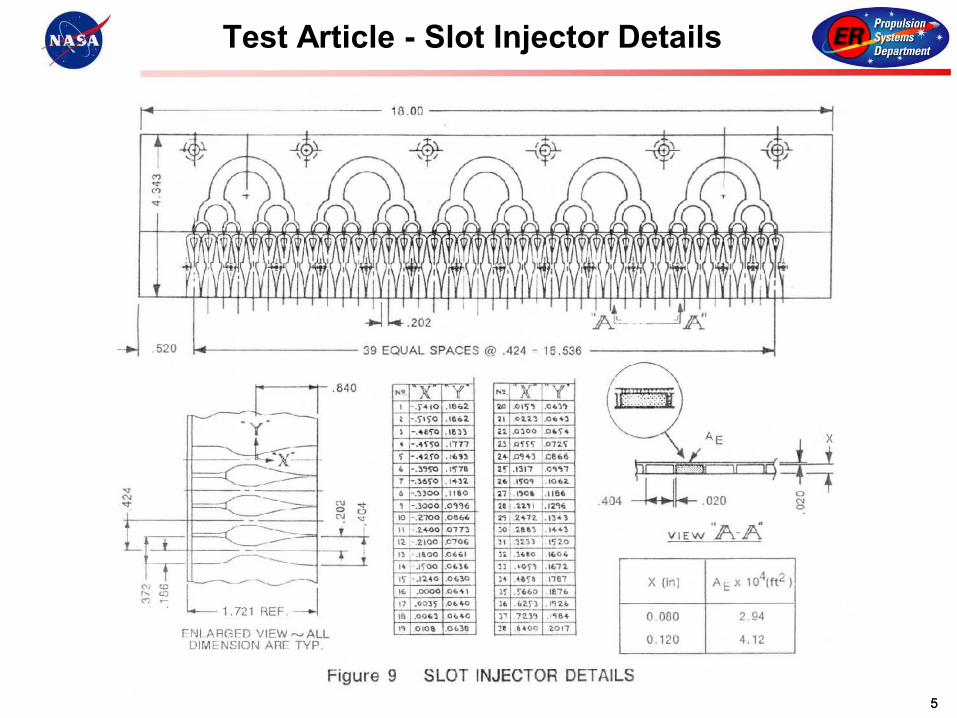
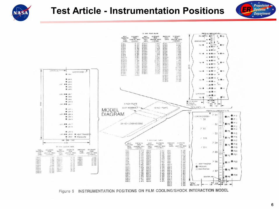
In this paper, the CFD simulation of the Calspan helium SSFC experiments is described. The hydrogencoolant work in Ref. 9 was modeled as well, and will be reported in a future paper. The Calspan experimentsemployed a reflected shock tunnel to generate a Mach 6.4 freestream flow around a test article. The freestreamgas was air during the helium cooling experiments (Refs. 6–8). Figures 1 and 2, reproduced from Ref. 8,depict the film cooling test article. The approach boundary layer for the freestream flow developed overa flat plate 32.28 inches long. The coolant flow was provided by an array of 40 coolant nozzles, each 0.12inches high, and 0.404 inches in width at their exit plane. The nozzles used an ideal 2-D contour designedto expand helium to Mach 3. The total step height at the injection plane is 0.14 inches, which includes the0.12 inch nozzle height and a 0.02 inch lip above the nozzles. Mixing of the film coolant and freestream flowsoccurred over another 17 inches of flat plate. Note that figure 1 shows the test article set up with a shockgenerator. The experimental data of interest in this work were the cases without the shock generator. Thehelium coolant injection was designed to be velocity-matched with the freestream flow.
Flowfield properties for the helium coolant cases modeled in this work are given in table 1. Run number4 was a flat plate case in which the 17 inch plate downstream of the injection plane was elevated to thesame height as the upstream 32.28 inch flat plate. Run number 43 was a case in the nominal film coolingconfiguration, but without coolant injection. Run numbers 44 through 47 had progressively increasingamounts of helium coolant flow injection.
III. Modeling Approach
The CFD analysis was performed using the Loci-CHEM CFD code, version 3.2-beta-10 (Ref.22). Loci-CHEM is a finite-volume flow solver for generalized grids developed at Mississippi State University in partthrough NASA and NSF funded efforts. It uses high resolution approximate Riemann solvers to solveturbulent flows with finite-rate chemistry. Loci-CHEM is comprised entirely of C and C++ code and issupported on all popular UNIX variants and compilers. Efficient parallel operation is facilitated by theLoci24 framework which exploits multi-threaded and MPI libraries. The code supports the use of a severaldifferent RANS turbulence models (Menter’s SST and BSL,25 Wilcox’s k-ω,26 a realizable k-ε,27 and Spalart-Allmaras28). Additionally, a hybrid RANS-LES mode is available for the SST, BSL and k-ω models.
In this work, three species were used: helium (for the coolant) and nitrogen and oxygen (as a basic airmodel). Thermodynamic properties were obtained using a standard partition function formulation whichcalculates the specific heats, internal energies and entropies of each individual perfect gas species. Laminar
3 of 21
American Institute of Aeronautics and Astronautics

Figure 1. Schematic diagram of test article and shock generator in the Calspan experiments, reproduced from AppendixA of Ref. 8. Note that, in this work, only experiments conducted without the shock generator present were simulated.Dimensions given are in inches.
Figure 2. Schematic diagram of injector section of the test article in the Calspan experiments, reproduced from figure13 of Ref. 8. Dimensions given are in inches.
4 of 21
American Institute of Aeronautics and Astronautics

transport property curve fits were obtained using TRANFIT in the CHEMKIN-II software package,29 andincorporated as inputs into Loci-CHEM. No finite-rate chemistry model was used, and the simulations wererun to steady state. Constant turbulent Prandtl and Schmidt numbers of 0.9 and 0.7, respectively, wereused in all turbulent CFD simulations. A constant wall temperature, Tw = 530◦R, was used for the no-slipwalls in all simulations.
IV. Results and Discussion
In this study, both 2-D and 3-D simulations were conducted. 2-D simulations of flat plate heating withoutcoolant flow are presented first, with a view toward understanding the basic grid resolution requirements andturbulence model characteristics. The 3-D simulations of the helium coolant nozzles, in which significant3-D viscous effects developed, are then discussed. Outflow properties from the 3-D nozzle simulations wereused to define coolant inflow profiles for 2-D simulations of the film cooling test article flowfield. The 2-D simulations investigated a number of coolant inflow approaches, turbulence models and compressibilitycorrections. Finally, 3-D simulations of the coupled coolant nozzles and film cooling domain are discussedand compared with the 2-D results.
IV.A. Flat Plate Heating Without Coolant Flow
In this section we examine baseline heating on the test article without film coolant present. All CFD resultspresented here are obtained with 2-D simulations. The x-y planar grid used for the simulations is shown infigure 3. Loci-CHEM is an unstructured 3-D code, and requires a fully 3-D grid. In the following discussions,2-D results were obtained by projecting a planar grid one cell in an orthogonal direction. The 2-D grid is ahybrid, unstructured mesh consisting of quadrilaterals near the test model surfaces, and triangles in the farfield. The inflow boundaries were set to a supersonic inflow boundary condition, while the outflow boundarywas set to a simple extrapolation. A slip wall boundary condition was applied for a short (0.01 inch) lengthof surface immediately downstream of the left inflow boundary, and upstream of the flat plate leading edge.The remaining surfaces were set to viscous no-slip walls.
The configuration shown in figure 3 applies to run numbers 43 through 47. For the flat plate heatingcase, run number 4, the backward facing step at the coolant injection plane was eliminated by elevating theplate downstream of the injection plane. The axial grid refinement near the injection plane is eliminated aswell.
As is evident in figure 3, the grid spacing is stretched vertically away from the test article surfaces.Near the leading edge of the flat plate, the axial grid spacing is also stretched to better capture the earlydevelopment of the flat plate boundary layer and the hypersonic viscous interaction in that region. In thebaseline grid, the vertical grid spacing was 1.0 × 10⁻⁴ inches next to the wall. The vertical spacing grewover 32 cells, and 0.02 inches, to 2.0× 10⁻³ inches, and again over 38 cells, and 0.4 inches, to 0.05 inches atthe edge of the quadrilateral/triangle transition. There were thus a total of 70 cells in the vertical direction.The axial grid spacing was 1.0 × 10⁻³ inches at the leading edge of the test article, and stretched over 50cells, and 1 inch, to a spacing of 0.1 inches. The hyperbolic tangent distribution was used, and the numberof grid cells specified was set to limit the stretching rate to ∼ 1.1.
The effect of different near-wall vertical spacing, as well as axial spacing, on the computed axial heat fluxprofile was examined. The SST turbulence model and default Wilcox compressibility correction were used.Calculations with wall vertical spacings of 2.0× 10⁻⁴ and 5.0× 10⁻⁵ inches, with an appropriate decrease orincrease in stretched cells, were performed. Typical heat flux values changed by 0.8% when the wall verticalspacing changed from 2.0× 10⁻⁴ to 1.0× 10⁻⁴ inches, and 0.4% going from 1.0× 10⁻⁴ to 5.0× 10⁻⁵ inches.This observation is consistent with the relatively low y+ values present: typical values for the baseline gridwere ∼ 0.3, and were ∼ 0.6 and ∼ 0.15 for the coarser and finer near-wall spacings, respectively. No effectwas seen by varying axial spacing. The axial spacing at the leading edge was held constant, but the largestaxial spacing downstream was tested at 0.05 and 0.2 inches.
The effect of turbulence model on the flat plate heating profiles was studied. Results are shown in theleft panel of figure 4 for several of the turbulence models available in Loci-CHEM. Calculated profiles for theSST, BSL, and the 1998 and 2008 versions of the Wilcox turbulence models are shown. The k-ε and Spalart-Allmaras turbulence models were also tested for this case, but did not result in heat flux profiles sufficientlyclose to the experimental data to consider using further in this study. The Wilcox compressibility correction,
5 of 21
American Institute of Aeronautics and Astronautics
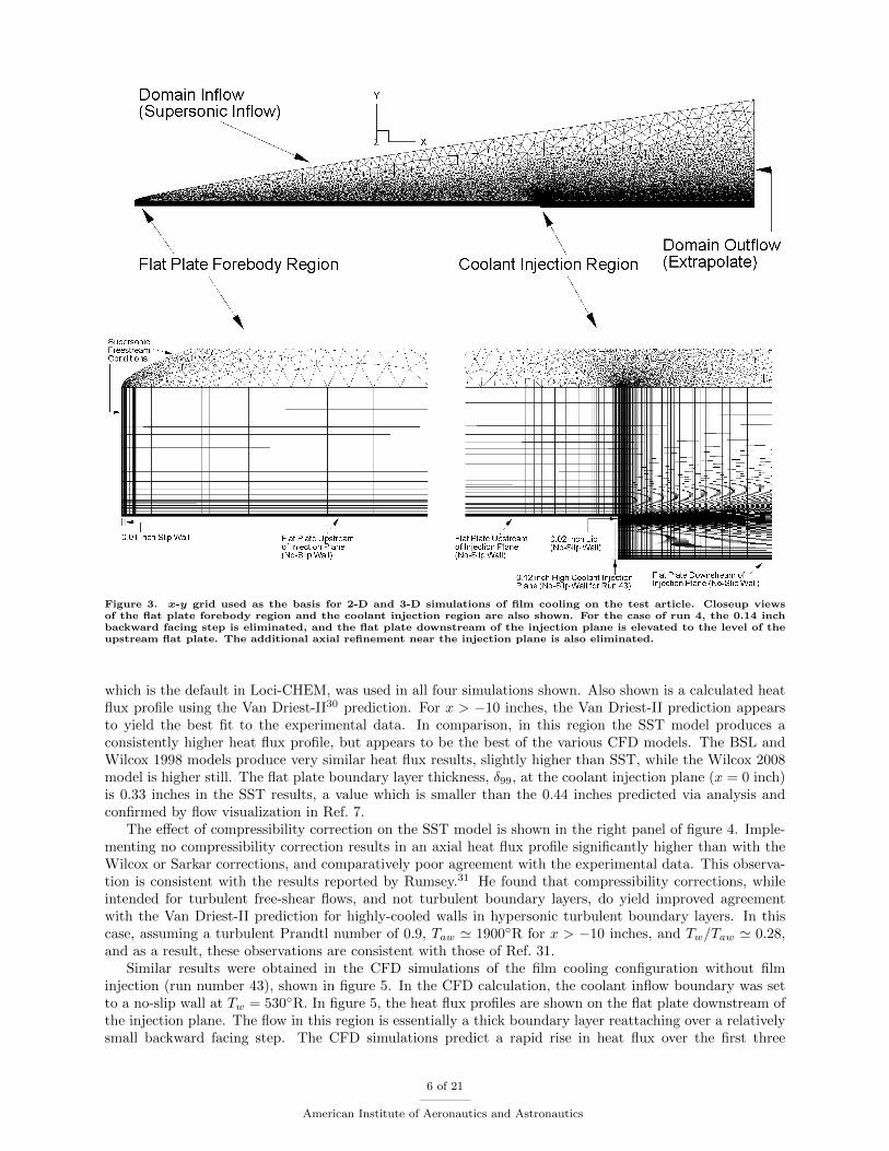
Figure 3. x-y grid used as the basis for 2-D and 3-D simulations of film cooling on the test article. Closeup viewsof the flat plate forebody region and the coolant injection region are also shown. For the case of run 4, the 0.14 inchbackward facing step is eliminated, and the flat plate downstream of the injection plane is elevated to the level of theupstream flat plate. The additional axial refinement near the injection plane is also eliminated.
which is the default in Loci-CHEM, was used in all four simulations shown. Also shown is a calculated heatflux profile using the Van Driest-II30 prediction. For x > −10 inches, the Van Driest-II prediction appearsto yield the best fit to the experimental data. In comparison, in this region the SST model produces aconsistently higher heat flux profile, but appears to be the best of the various CFD models. The BSL andWilcox 1998 models produce very similar heat flux results, slightly higher than SST, while the Wilcox 2008model is higher still. The flat plate boundary layer thickness, δ99, at the coolant injection plane (x = 0 inch)is 0.33 inches in the SST results, a value which is smaller than the 0.44 inches predicted via analysis andconfirmed by flow visualization in Ref. 7.
The effect of compressibility correction on the SST model is shown in the right panel of figure 4. Imple-menting no compressibility correction results in an axial heat flux profile significantly higher than with theWilcox or Sarkar corrections, and comparatively poor agreement with the experimental data. This observa-tion is consistent with the results reported by Rumsey.31 He found that compressibility corrections, whileintended for turbulent free-shear flows, and not turbulent boundary layers, do yield improved agreementwith the Van Driest-II prediction for highly-cooled walls in hypersonic turbulent boundary layers. In thiscase, assuming a turbulent Prandtl number of 0.9, Taw ' 1900◦R for x > −10 inches, and Tw/Taw ' 0.28,and as a result, these observations are consistent with those of Ref. 31.
Similar results were obtained in the CFD simulations of the film cooling configuration without filminjection (run number 43), shown in figure 5. In the CFD calculation, the coolant inflow boundary was setto a no-slip wall at Tw = 530◦R. In figure 5, the heat flux profiles are shown on the flat plate downstream ofthe injection plane. The flow in this region is essentially a thick boundary layer reattaching over a relativelysmall backward facing step. The CFD simulations predict a rapid rise in heat flux over the first three
6 of 21
American Institute of Aeronautics and Astronautics
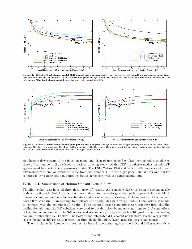
Figure 4. Effect of turbulence model (left panel) and compressibility correction (right panel) on calculated axial heatflux profiles for run number 4. The Wilcox compressibility correction was used for all four turbulence models in theleft panel. The turbulence model used in the right panel is SST.
Figure 5. Effect of turbulence model (left panel) and compressibility correction (right panel) on calculated axial heatflux profiles for run number 43. The Wilcox compressibility correction was used for all four turbulence models in theleft panel. The turbulence model used in the right panel is SST.
step-heights downstream of the injection plane, and then relaxation to flat plate heating values similar tothose of run number 4 (i.e., without a backward facing step). Of the CFD turbulence models tested, SSTagain agreed best with the experimental data. The BSL, Wilcox 1998 and Wilcox 2008 models yield heatflux results with similar trends to those from run number 4. In the right panel, the Wilcox and Sarkarcompressibility corrections again produce better agreement with the experimental data.
IV.B. 3-D Simulations of Helium Coolant Nozzle Flow
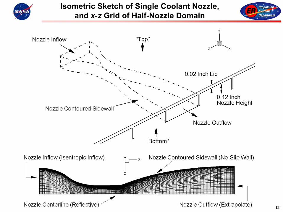
The film coolant was injected through an array of nozzles. An isometric sketch of a single coolant nozzleis shown in figure 6. Ref. 7 states that the nozzle contour was designed to ideally expand helium to Mach3 using a combined method-of-characteristics and viscous analysis strategy. 2-D simulations of the coolantnozzle flow were run in an attempt to duplicate the original design strategy, and 3-D simulations were runto compare with the experimental results. These isolated nozzle simulations were separate from the filmcooling domain, and the 3-D solutions were used to obtain inflow boundary conditions for 2-D simulationsof the film cooling domain. The 3-D nozzle grid is completely integrated with a 3-D grid of the film coolingdomain in subsection IV.D below. The isolated and integrated 3-D coolant nozzle flowfields are very similar,except for minor differences that creep up through the boundary layers near the nozzle exit planes.
The x-z planar half-nozzle grid used as the basis for constructing both the 2-D and 3-D nozzle grids is
7 of 21
American Institute of Aeronautics and Astronautics

Figure 6. Isometric sketch of a single coolant nozzle
Figure 7. 229 × 85 cell half-nozzle grid in the x-z plane.
shown in figure 7. The grid was 229 cells in the axial direction, and 85 cells in the transverse direction.The nozzle sidewall contour was generated from the “X” and “Y” coordinates shown in figure 2, with splineinterpolation between the points. This contour was set to a no-slip wall. The nozzle inflow boundary was setto an isentropic inflow boundary condition with stagnation pressure and temperature specified. The nozzleoutflow exit plane was set to simple extrapolation. The nozzle centerline was set to a reflective plane.
The grid spacing near the nozzle contour was consistent with the values used in the previous subsection:1.0× 10⁻⁴ inches off the wall, and increasing through a hyperbolic tangent distribution to 2.0× 10⁻³ inchesover 32 cells, and 0.02 inches. The 2-D grid was constructed by projecting the grid in the x-z plane one cell,for 0.12 inches, in the y-direction. Symmetry boundary conditions were specified on the top and bottomsurfaces. The 3-D grid was constructed by projecting the x-z planar grid 90 cells, for 0.12 inches, in they-direction. No-slip walls were specified for the top and bottom surfaces. The near wall grid spacing on bothends of this projection was consistent with the values described above.
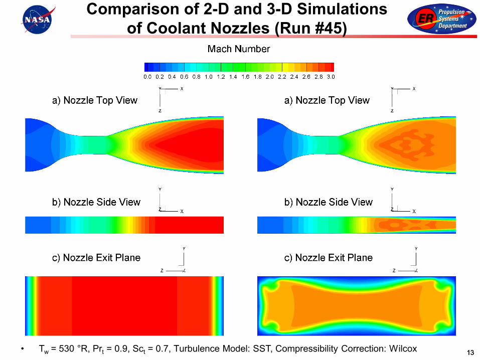
Figure 8 compares the 2-D and 3-D simulations of the nozzle flow. The nozzle stagnation conditions atthe inflow plane were set to those for run number 45 of Ref. 8: p0 = 18.32 psia and T0 = 530 ◦R. In allimages shown, the solution was reflected across the nozzle centerline to depict the actual physical situationmore clearly. The nozzle top view (a) presents a constant-y plane at y = 0.06 inches, halfway up the 0.12inch height of the nozzle. The nozzle side view (b) presents a constant-z plane at z = 0 inches (the nozzlecenterline), and the nozzle exit plane view (c) is at x = 0 inch, the end the nozzle.
The SST turbulence model with the Wilcox compressibility correction was used for both the 2-D and the3-D simulations. The default k and ω values for the isentropic inflow boundary condition are 0.001 and 9000,
8 of 21
American Institute of Aeronautics and Astronautics

Figure 8. Top, side and exit plane views showing Mach number contours in the helium coolant nozzles. The top view(a) depicts the y = 0.06 inch plane, halfway up the nozzle. The side view (b) shows the z = 0 inch plane, along thenozzle centerline. The nozzle exit plane view shows the x = 0 inch plane; it is not to scale with the top and side views.Left panel: idealized 2-D nozzle flow with slip walls on the top and bottom surfaces. Right panel: actual 3-D nozzleflow with no-slip walls on top and bottom surfaces. Helium inflow conditions are those for run45: p0 = 18.32 psia, T0
= 530 ◦R. Turbulence Model: SST
Figure 9. Plots showing nozzle centerline (z = 0, y = 0.06 inches) flow Mach number (left panel) and pressure ratio(right panel) as a function of axial displacement from the nozzle exit plane. 3-D nozzle flow with no-slip wall boundaryconditions on the top and bottom surfaces is compared to idealized 2-D nozzle flow with symmetry boundary conditionson the top and bottom surfaces. Helium inflow conditions are those for run number 45: p0 = 18.32 psia, T0 = 530 ◦R.Turbulence Model: SST
9 of 21
American Institute of Aeronautics and Astronautics

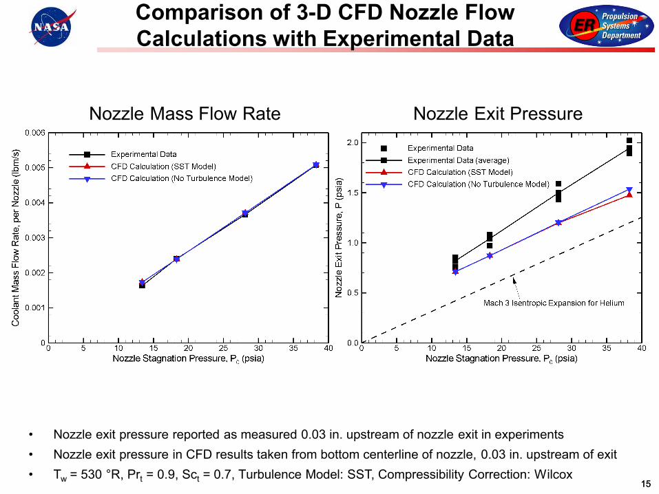
Figure 10. Plots comparing 3-D CFD model results with the experimental data for the helium coolant nozzles. Leftpanel: coolant nozzle mass flow rate, per nozzle. Right panel: nozzle exit pressure.
respectively, resulting in an inflow turbulence intensity of ∼ 2 × 10⁻⁸. For this geometry, and these inflowturbulence intensities, none of the turbulence models generated turbulence intensities sufficient to alter theflow from laminar flow for the stagnation conditions of run numbers 44–46. There are some small differencesbetween turbulent and laminar simulations for the conditions of run number 47.
It is evident from the left panel of figure 8 that the 2-D CFD results effectively reproduce the originaldesign strategy for the helium coolant nozzles. The ideal nozzle wall contour produces a relatively uniformMach 3 core flow free of shock waves. This is also evident from figure 9, in which Mach number (left panel)and pressure ratio, P/P0, (right panel) are plotted along the nozzle centerline (z = 0, y = 0.06 inches). TheMach number is slightly higher than Mach 3, and the pressure ratio slightly lower than 0.03125 (the nominalvalue for an isentropic expansion of helium to Mach 3), for the final half-inch of the nozzle before the exitplane. The nozzle sidewall boundary layer thickness, δ99, at the exit plane is 0.026 inches in the CFD results,a value which is slightly larger than the 0.024 inches predicted in Ref. 7.
In contrast, it is seen in the right panel of figure 8 that, in the 3-D simulation, viscous effects on the topand bottom walls have a significant effect on the core flow. Boundary layer growth constricts the core flow,and prevents expansion of the helium to Mach 3. The effects of weak oblique shocks, emanating from theboundary layers, are evident in the nozzle top and side views. The boundary layer growth is largest along thenozzle centerline. The core Mach number is ∼ 2.7 over the final half-inch of the nozzle, with a correspondingpressure ratio of 0.046−0.049 (figure 9). Similar 3-D effects were also observed in the computational studyof Ref. 16.
A comparison of the CFD results of the nozzles with the experimental measurements for run numbers44–47 is shown in figure 10. Coolant mass flow rate, per nozzle, is shown in the left panel, and nozzle exitpressure is shown in the right panel. The method by which the coolant mass flow rate was experimentallydetermined is described in detail in Ref. 8. The nozzle exit pressure was measured in the coolant nozzlesat an axial location 0.03 inches upstream of the nozzle exit plane. Geometry strongly suggests that themeasurement was on the bottom surface of the coolant nozzles, however the exact size and spanwise locationof the pressure transducers within the nozzle is uncertain. From examination of the data tables for each run(Appendix A of Ref. 8), it appears that the reported exit pressure was the average of the measured valuesin five different nozzles.
In figure 10, there is good agreement between the experimental mass flow rate per nozzle and the valuecalculated from the 3-D CFD results. However, there are significant discrepancies between the experimentalnozzle exit pressures and the results from the CFD calculations. The pressure shown in figure 10 for theCFD calculations was extracted along the nozzle centerline, on the bottom (y = 0 inch) surface, 0.03inches upstream from the exit plane. The CFD nozzle exit pressures range from 13% to 24% less thanthe experimental values. Figure 10 shows, as discussed previously, that the SST model did not generateturbulence intensities sufficient to change the pressure from the corresponding non-turbulent (laminar flow)results with the exception of the highest-pressure condition (run number 47). Note that both the experimentaland the CFD results have nozzle exit pressures significantly higher than those predicted for an ideal, isentropic
10 of 21
American Institute of Aeronautics and Astronautics
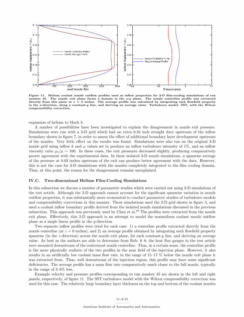
Figure 11. Helium coolant nozzle outflow profiles used as inflow properties for 2-D film-cooling simulations of runnumber 45. The nozzle exit plane forms a domain in the z-y plane. The nozzle centerline profile was extracteddirectly from this plane at z = 0 inches. The average profile was calculated by integrating each flowfield propertyin the z-direction, along a constant-y line, and deriving an average value. Turbulence model: SST, with the Wilcoxcompressibility correction.
expansion of helium to Mach 3.A number of possibilities have been investigated to explain the disagreement in nozzle exit pressure.
Simulations were run with a 3-D grid which had an extra 0.34 inch straight duct upstream of the inflowboundary shown in figure 7, in order to assess the effect of additional boundary layer development upstreamof the nozzles. Very little effect on the results was found. Simulations were also run on the original 3-Dnozzle grid using inflow k and ω values set to produce an inflow turbulence intensity of 1%, and an inflowviscosity ratio µt/µ = 100. In these cases, the exit pressures decreased slightly, producing comparativelypoorer agreement with the experimental data. In these isolated 3-D nozzle simulations, a spanwise averageof the pressure at 0.03 inches upstream of the exit can produce better agreement with the data. However,this is not the case for 3-D simulations with the nozzles completely integrated to the film cooling domain.Thus, at this point, the reason for the disagreement remains unexplained.
IV.C. Two-dimensional Helium Film-Cooling Simulations
In this subsection we discuss a number of parametric studies which were carried out using 2-D simulations ofthe test article. Although the 2-D approach cannot account for the significant spanwise variation in nozzleoutflow properties, it was substantially more economical to conduct parametric studies of turbulence modelsand compressibility corrections in this manner. These simulations used the 2-D grid shown in figure 3, andused a coolant inflow boundary profile derived from the isolated nozzle simulations discussed in the previoussubsection. This approach was previously used by Chen et al.16 The profiles were extracted from the nozzleexit plane. Effectively, this 2-D approach is an attempt to model the nonuniform coolant nozzle outflowplane as a single linear profile in the y-direction.
Two separate inflow profiles were tried for each case: 1) a centerline profile extracted directly from thenozzle centerline (at z = 0 inches), and 2) an average profile obtained by integrating each flowfield propertyspanwise (in the z-direction) across the nozzle exit plane, for each constant-y line, and deriving an averagevalue. As best as the authors are able to determine from Refs. 6–8, the heat flux gauges in the test articlewere mounted downstream of the centermost nozzle centerline. Thus, in a certain sense, the centerline profileis the more physically realistic of the two profiles in the near field of the injection plane. However, it alsoresults in an artificially low coolant mass flow rate, in the range of 15–17 % below the nozzle exit plane itwas extracted from. Thus, well downstream of the injection region, this profile may have some significantdeficiencies. The average profile has a mass flow rate comparatively much closer to the full nozzle, typicallyin the range of 3–6% less.
Example velocity and pressure profiles corresponding to run number 45 are shown in the left and rightpanels, respectively, of figure 11. The SST turbulence model with the Wilcox compressibility correction wasused for this case. The relatively large boundary layer thickness on the top and bottom of the coolant nozzles
11 of 21
American Institute of Aeronautics and Astronautics
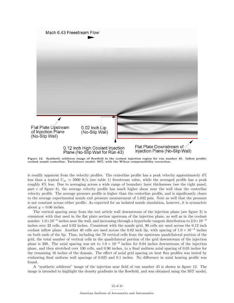
Figure 12. Synthetic schlieren image of flowfield in the coolant injection region for run number 45. Inflow profile:coolant nozzle centerline. Turbulence model: SST, with the Wilcox compressibility correction.
is readily apparent from the velocity profiles. The centerline profile has a peak velocity approximately 4%less than a typical U∞ ' 5000 ft/s (see table 1) freestream value, while the averaged profile has a peakroughly 8% less. Due to averaging across a wide range of boundary layer thicknesses (see the right panel,part c of figure 8), the average velocity profile has much higher shear near the wall than the centerlinevelocity profile. The average pressure profile is higher than the centerline profile, and is significantly closerto the average experimental nozzle exit pressure measurement of 1.042 psia. Note as well that the pressureis not constant across either profile. As expected for an isolated nozzle simulation, however, it is symmetricabout y = 0.06 inches.
The vertical spacing away from the test article wall downstream of the injection plane (see figure 3) isconsistent with that used in the flat plate section upstream of the injection plane, as well as in the coolantnozzles: 1.0×10⁻⁴ inches near the wall, and increasing through a hyperbolic tangent distribution to 2.0×10⁻³
inches over 32 cells, and 0.02 inches. Consistent with the nozzle grid, 90 cells are used across the 0.12 inchcoolant inflow plane. Another 40 cells are used across the 0.02 inch lip, with spacing of 1.0 × 10⁻⁴ incheson both ends of the lip. Thus, including the 70 vertical cells from the upstream quadrilateral portion of thegrid, the total number of vertical cells in the quadrilateral portion of the grid downstream of the injectionplane is 200. The axial spacing was set to 1.0 × 10⁻³ inches for 0.04 inches downstream of the injectionplane, and then stretched over 100 cells, and 0.96 inches, to a final uniform axial spacing of 0.05 inches forthe remaining 16 inches of the domain. The effect of axial grid spacing on heat flux profiles was tested byevaluating final uniform wall spacings of 0.025 and 0.1 inches. No difference in axial heating profile wasfound.
A “synthetic schlieren” image of the injection near field of run number 45 is shown in figure 12. Theimage is intended to highlight the density gradients in the flowfield, and was obtained using the SST model,
12 of 21
American Institute of Aeronautics and Astronautics
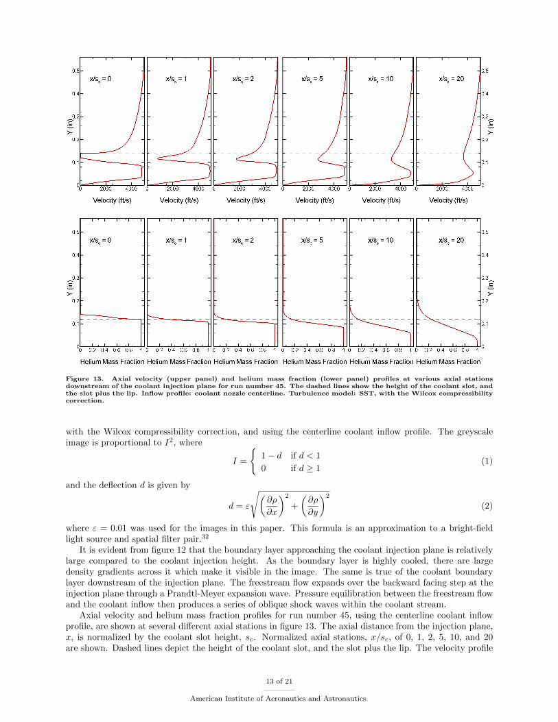
Figure 13. Axial velocity (upper panel) and helium mass fraction (lower panel) profiles at various axial stationsdownstream of the coolant injection plane for run number 45. The dashed lines show the height of the coolant slot, andthe slot plus the lip. Inflow profile: coolant nozzle centerline. Turbulence model: SST, with the Wilcox compressibilitycorrection.
with the Wilcox compressibility correction, and using the centerline coolant inflow profile. The greyscaleimage is proportional to I2, where
I =
{1− d if d < 1
0 if d ≥ 1(1)
and the deflection d is given by
d = ε
√(∂ρ
∂x
)2
+
(∂ρ
∂y
)2
(2)
where ε = 0.01 was used for the images in this paper. This formula is an approximation to a bright-fieldlight source and spatial filter pair.32
It is evident from figure 12 that the boundary layer approaching the coolant injection plane is relativelylarge compared to the coolant injection height. As the boundary layer is highly cooled, there are largedensity gradients across it which make it visible in the image. The same is true of the coolant boundarylayer downstream of the injection plane. The freestream flow expands over the backward facing step at theinjection plane through a Prandtl-Meyer expansion wave. Pressure equilibration between the freestream flowand the coolant inflow then produces a series of oblique shock waves within the coolant stream.
Axial velocity and helium mass fraction profiles for run number 45, using the centerline coolant inflowprofile, are shown at several different axial stations in figure 13. The axial distance from the injection plane,x, is normalized by the coolant slot height, sc. Normalized axial stations, x/sc, of 0, 1, 2, 5, 10, and 20are shown. Dashed lines depict the height of the coolant slot, and the slot plus the lip. The velocity profile
13 of 21
American Institute of Aeronautics and Astronautics

Figure 14. Effect of turbulence model on 2-D calculated axial heat flux profiles for run number 45. The Wilcoxcompressibility correction, which is the default one in Loci-CHEM, was used for all four turbulence models. Left panel:coolant nozzle centerline inflow profile. Right panel: coolant nozzle average inflow profile.
Figure 15. Effect of turbulence model on 2-D calculated axial heat flux profiles for run number 47. The Wilcoxcompressibility correction, which is the default one in Loci-CHEM, was used for all four turbulence models. Left panel:coolant nozzle centerline inflow profile. Right panel: coolant nozzle average inflow profile.
at the injection plane (x/sc = 0) is as expected: the centerline coolant velocity profile from the left panelof figure 11 may be seen in the lower part of the profile from y = 0 to 0.12 inches. The velocity is zeroalong the lip wall surface, and then rapidly increases toward the freestream value through a comparativelylarge turbulent boundary layer profile. The incoming boundary layer thickness in the coolant stream isapproximately twice the lip width, while the freestream turbulent boundary layer thickness is over 16 timeslarger than the lip. At one slot height downstream (x/sc = 1), the velocity profile is similar to that at theinjection plane, but a wake-like mixing of the two streams is evident. Due to the size of the boundary layersin the two streams, this wake-like mixing initially occurs at velocities much lower than the U∞ ' 5000 ft/sfreestream and coolant core velocities. At x/sc = 1 the velocity defect (with respect to the freestream) isquite large, 84%. It is 65% at x/sc = 2, 45% at x/sc = 5, and 35% at x/sc = 10. At x/sc = 20, the defect isstill evident, though at this point the coolant stream core velocity has decreased to roughly 4500 ft/s, andthe coolant boundary layer on the lower wall has fully transitioned to a turbulent profile. By this point, itmay be seen from the lower panel that the freestream gas has penetrated about two-thirds of the way acrossthe coolant flow. Thus, in contrast to a classic mixing layer velocity profile, the near-field turbulent mixingbetween the coolant and freestream here is dominated by a wake-like mixing process. The same phenomenais seen in the 2-D results for the other film cooling cases.
The effect of coolant inflow profile and turbulence model on the axial film cooling heating profiles wasstudied. Results are shown in figures 14 (run number 45) and 15 (run number 47) for the SST, BSL, and the
14 of 21
American Institute of Aeronautics and Astronautics

1998 and 2008 versions of the Wilcox turbulence models. The default Wilcox compressibility correction wasused for all turbulence models. It should be noted that for each run number and turbulence model studied, aseparate nozzle case was run using that turbulence model. Results using the centerline coolant inflow profileare presented in the left panels of figures 14 and 15, while results using the average coolant inflow profile aredepicted in the right panels. Also shown in the figures is a reference flat plate heating profile used in Ref. 7.The equation is
q(x) = 9.14− 0.119x+ 0.0034x2 (3)
where q is in BTU/ft2-s and x is in inches. As it is based on a nominal freestream condition, this relationdoes not exactly represent the flat plate heating for a specific run. However, it does provide a representativereference point in the figures.
It may be seen from figures 14 and 15 that, in both the CFD simulations and the experimental data,there is initially a length of minimal heat flux in which the coolant at the wall is uncontaminated by thefreestream gas (i.e., the adiabatic cooling length). Note that neither coolant inflow profile in the CFD resultsfor run number 45 exactly predicts the adiabatic cooling length in the experimental data, while the CFDresults for run number 47 predict this length more accurately. For both runs, the centerline coolant profiledoes a better job at predicting this length than the average coolant profile. However, the centerline inflowprofile also has a comparatively worse agreement with the slope of the data in the developed flow region (thedownstream region in which the freestream gas has mixed to the wall and is increasing the heat flux). Thisis likely due to the lower coolant mass flow rate of this profile. Overall, neither coolant inflow profile, withany of the turbulence models, produced good agreement with the experimental data in the developed flowregion for run number 45, while, again the agreement for run number 47 is considerably better. It appearsthat the experimental data for run number 45 exhibit, at the end of the adiabatic cooling length, a sharprise in heat flux, followed by a gradual relaxation of the slope. The CFD calculations fail to predict thedecreased slope in the experimental heat flux profile after the initial rise. The reason for the poor agreementfor run number 45 is currently unknown.
The SST, BSL and 2008 Wilcox models produce similar heat flux profiles. All three have nearly identicaladiabatic cooling lengths, with relatively minor differences in the slope of the heat flux profile in the developedflow region. For both runs, the 1998 Wilcox model consistently produces a longer adiabatic cooling lengththan the other three models, and a more gradual slope for the heat flux profile in the developed flow region.
The effect of turbulence model compressibility correction on the film cooling heat flux profiles was alsoinvestigated. Results are shown in figure 16 for run number 45, and figure 17 for run number 47. Allsimulations were run with the SST turbulence model. Again, for each run number and compressibilityimplementation, a separate nozzle case was run. As was seen in the earlier flat plate heating results,implementing either the Wilcox or Sarkar corrections results in a lower heat flux profile than the use of nocorrection. The Sarkar correction yields the lowest slope of the heat flux profile in the developed region, andhas the best agreement with the experimental data. The two coolant inflow profiles exhibit the same trendshere as was the case in the turbulence model comparisons above.
IV.D. Three-dimensional Helium Film-Cooling Simulations
It is evident from the previous section that the flow nonuniformities present in the coolant outflow makeaccurate 2-D simulations of the Calspan experiments a challenging task. After gaining insight and experiencewith the 2-D simulations, we conducted 3-D simulations of the film-cooling experiments. The 3-D grid wasgenerated from the 2-D x-y grid shown in figure 3. Spanwise, the computational domain comprises half of asingle coolant nozzle (0.202 inches at the nozzle exit, and see figure 7), plus half of the wall width betweenthe coolant nozzles (0.01 inches), for a total spanwise width of 0.212 inches. By setting reflective boundaryconditions on both sides of the spanwise direction, effectively an infinite array of cooling nozzles is simulated.In this approach, flowfield symmetry across the nozzle centerline, and from nozzle to nozzle, is assumed. 100cells total were used in the spanwise direction, with 85 dedicated to the half-nozzle, and 15 to half of theinter-nozzle wall. Clustering was used in the vicinity of the nozzle sidewall (see figure 7). This clusteringwas relaxed away from the coolant nozzles: for x > 1 inch, the spanwise spacing was uniform at 2.12× 10⁻³
inches. The resulting 3-D grid comprised ∼ 16.5 million cells.The previous sections have shown that the SST turbulence model with a compressibility correction
performed reasonably well at predicting flat plate heat flux distribution. Although none of the turbulencemodels did a consistently good job of predicting the film cooling data in the 2-D film cooling simulations,
15 of 21
American Institute of Aeronautics and Astronautics
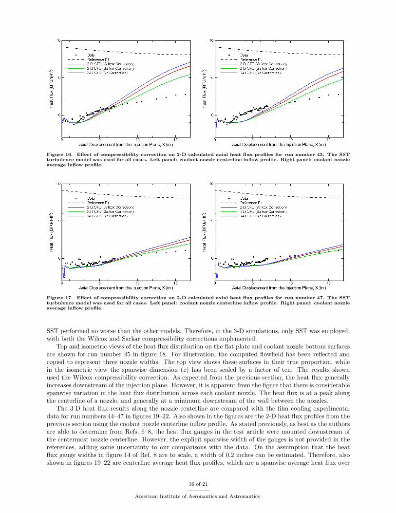
Figure 16. Effect of compressibility correction on 2-D calculated axial heat flux profiles for run number 45. The SSTturbulence model was used for all cases. Left panel: coolant nozzle centerline inflow profile. Right panel: coolant nozzleaverage inflow profile.
Figure 17. Effect of compressibility correction on 2-D calculated axial heat flux profiles for run number 47. The SSTturbulence model was used for all cases. Left panel: coolant nozzle centerline inflow profile. Right panel: coolant nozzleaverage inflow profile.
SST performed no worse than the other models. Therefore, in the 3-D simulations, only SST was employed,with both the Wilcox and Sarkar compressibility corrections implemented.
Top and isometric views of the heat flux distribution on the flat plate and coolant nozzle bottom surfacesare shown for run number 45 in figure 18. For illustration, the computed flowfield has been reflected andcopied to represent three nozzle widths. The top view shows these surfaces in their true proportion, whilein the isometric view the spanwise dimension (z) has been scaled by a factor of ten. The results shownused the Wilcox compressibility correction. As expected from the previous section, the heat flux generallyincreases downstream of the injection plane. However, it is apparent from the figure that there is considerablespanwise variation in the heat flux distribution across each coolant nozzle. The heat flux is at a peak alongthe centerline of a nozzle, and generally at a minimum downstream of the wall between the nozzles.
The 3-D heat flux results along the nozzle centerline are compared with the film cooling experimentaldata for run numbers 44–47 in figures 19–22. Also shown in the figures are the 2-D heat flux profiles from theprevious section using the coolant nozzle centerline inflow profile. As stated previously, as best as the authorsare able to determine from Refs. 6–8, the heat flux gauges in the test article were mounted downstream ofthe centermost nozzle centerline. However, the explicit spanwise width of the gauges is not provided in thereferences, adding some uncertainty to our comparisons with the data. On the assumption that the heatflux gauge widths in figure 14 of Ref. 8 are to scale, a width of 0.2 inches can be estimated. Therefore, alsoshown in figures 19–22 are centerline average heat flux profiles, which are a spanwise average heat flux over
16 of 21
American Institute of Aeronautics and Astronautics
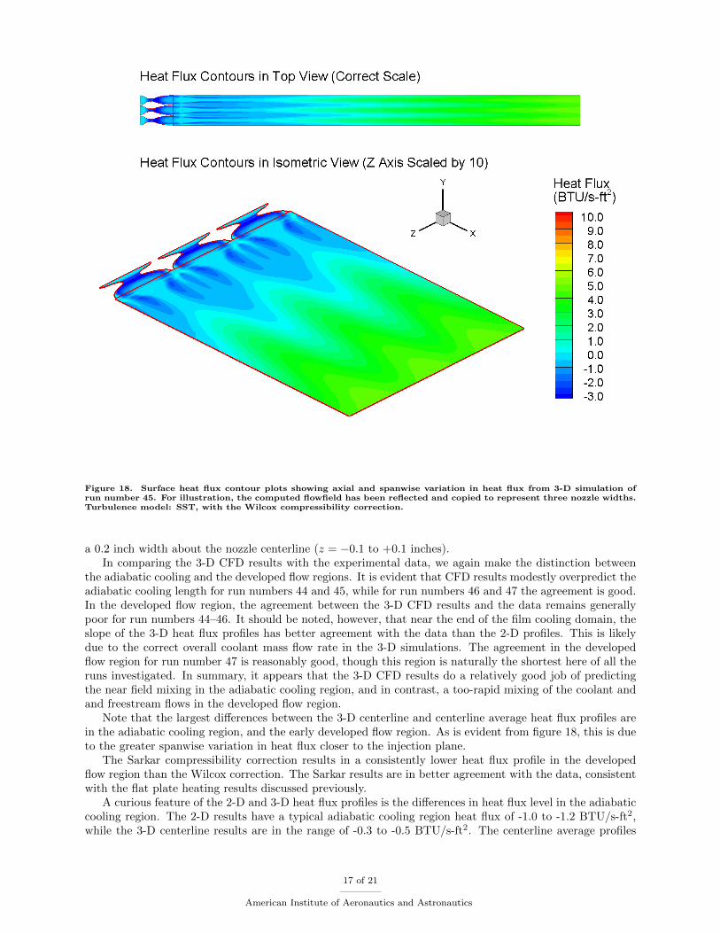
Figure 18. Surface heat flux contour plots showing axial and spanwise variation in heat flux from 3-D simulation ofrun number 45. For illustration, the computed flowfield has been reflected and copied to represent three nozzle widths.Turbulence model: SST, with the Wilcox compressibility correction.
a 0.2 inch width about the nozzle centerline (z = −0.1 to +0.1 inches).In comparing the 3-D CFD results with the experimental data, we again make the distinction between
the adiabatic cooling and the developed flow regions. It is evident that CFD results modestly overpredict theadiabatic cooling length for run numbers 44 and 45, while for run numbers 46 and 47 the agreement is good.In the developed flow region, the agreement between the 3-D CFD results and the data remains generallypoor for run numbers 44–46. It should be noted, however, that near the end of the film cooling domain, theslope of the 3-D heat flux profiles has better agreement with the data than the 2-D profiles. This is likelydue to the correct overall coolant mass flow rate in the 3-D simulations. The agreement in the developedflow region for run number 47 is reasonably good, though this region is naturally the shortest here of all theruns investigated. In summary, it appears that the 3-D CFD results do a relatively good job of predictingthe near field mixing in the adiabatic cooling region, and in contrast, a too-rapid mixing of the coolant andand freestream flows in the developed flow region.
Note that the largest differences between the 3-D centerline and centerline average heat flux profiles arein the adiabatic cooling region, and the early developed flow region. As is evident from figure 18, this is dueto the greater spanwise variation in heat flux closer to the injection plane.
The Sarkar compressibility correction results in a consistently lower heat flux profile in the developedflow region than the Wilcox correction. The Sarkar results are in better agreement with the data, consistentwith the flat plate heating results discussed previously.
A curious feature of the 2-D and 3-D heat flux profiles is the differences in heat flux level in the adiabaticcooling region. The 2-D results have a typical adiabatic cooling region heat flux of -1.0 to -1.2 BTU/s-ft2,while the 3-D centerline results are in the range of -0.3 to -0.5 BTU/s-ft2. The centerline average profiles
17 of 21
American Institute of Aeronautics and Astronautics
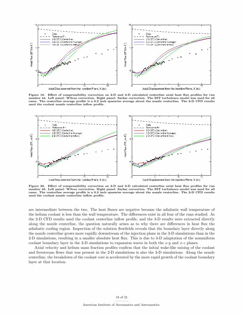
Figure 19. Effect of compressibility correction on 2-D and 3-D calculated centerline axial heat flux profiles for runnumber 44. Left panel: Wilcox correction. Right panel: Sarkar correction. The SST turbulence model was used for allcases. The centerline average profile is a 0.2 inch spanwise average about the nozzle centerline. The 2-D CFD resultsused the coolant nozzle centerline inflow profile.
Figure 20. Effect of compressibility correction on 2-D and 3-D calculated centerline axial heat flux profiles for runnumber 45. Left panel: Wilcox correction. Right panel: Sarkar correction. The SST turbulence model was used for allcases. The centerline average profile is a 0.2 inch spanwise average about the nozzle centerline. The 2-D CFD resultsused the coolant nozzle centerline inflow profile.
are intermediate between the two. The heat fluxes are negative because the adiabatic wall temperature ofthe helium coolant is less than the wall temperature. The differences exist in all four of the runs studied. Asthe 2-D CFD results used the coolant centerline inflow profile, and the 3-D results were extracted directlyalong the nozzle centerline, the question naturally arises as to why there are differences in heat flux theadiabatic cooling region. Inspection of the solution flowfields reveals that the boundary layer directly alongthe nozzle centerline grows more rapidly downstream of the injection plane in the 3-D simulations than in the2-D simulations, resulting in a smaller absolute heat flux. This is due to 3-D adaptation of the nonuniformcoolant boundary layer in the 3-D simulations to expansion waves in both the x-y and x-z planes.
Axial velocity and helium mass fraction profiles confirm that the initial wake-like mixing of the coolantand freestream flows that was present in the 2-D simulations is also the 3-D simulations. Along the nozzlecenterline, the breakdown of the coolant core is accelerated by the more rapid growth of the coolant boundarylayer at that location.
18 of 21
American Institute of Aeronautics and Astronautics

Figure 21. Effect of compressibility correction on 2-D and 3-D calculated centerline axial heat flux profiles for runnumber 46. Left panel: Wilcox correction. Right panel: Sarkar correction. The SST turbulence model was used for allcases. The centerline average profile is a 0.2 inch spanwise average about the nozzle centerline. The 2-D CFD resultsused the coolant nozzle centerline inflow profile.
Figure 22. Effect of compressibility correction on 2-D and 3-D calculated centerline axial heat flux profiles for runnumber 47. Left panel: Wilcox correction. Right panel: Sarkar correction. The SST turbulence model was used for allcases. The centerline average profile is a 0.2 inch spanwise average about the nozzle centerline. The 2-D CFD resultsused the coolant nozzle centerline inflow profile.
V. Summary
In an effort to benchmark Loci-CHEM for SSFC flowfields for the J-2X program, SSFC experimentsconducted at Calspan in the late 1980s and early 1990s were simulated and analyzed. These experimentswere selected for study because they were well-documented, readily available, and physically relevant toSSFC on the J-2X NE. However, in the course of this investigation, some key knowledge gaps about theexperiments arose: specifically, the precise size and spanwise location of the coolant nozzle exit pressuretransducers, and the spanwise width of the heat flux gauges.
This study investigated the experiments in a building-block approach, first simulating the flat plateheating results without film cooling present on a 2-D grid. The hypersonic turbulent boundary layers presentin the experiments were highly cooled, and compressibility corrections were found to improve agreementbetween the CFD heat flux results and the experimental data.
Next, a single coolant nozzle was simulated on a 3-D grid, with a view toward gaining insight in thatflowfield, as well as providing a nozzle exit plane from which physically relevant profiles could be extracted asinflow boundary conditions for 2-D film cooling simulations. 3-D viscous effects were observed in the coolantnozzles, leading to significant flow nonuniformities at the nozzle exit plane. The experimental coolant massflow rates were well-predicted by the CFD simulations. However, there were unresolved discrepancies between
19 of 21
American Institute of Aeronautics and Astronautics
the CFD results and nozzle exit pressure data.The effect of several CFD modeling parameters were then investigated using 2-D simulations of the film
cooling domain. Given the coolant nozzle flow nonuniformities, reducing the nozzle exit plane to a singlelinear profile for an inflow boundary is a crude approximation. However, two different coolant inflow profileapproaches were investigated: a coolant nozzle centerline profile, and a coolant nozzle average profile. Thecenterline profile produced a better prediction of the adiabatic cooling length than the average profile, buta poorer prediction of the slope of the heat flux profile in the developed region of the flowfield. The SST,BSL and 2008 Wilcox turbulence models performed similarly, and compressibility corrections again improvedagreement with the experimental data.
After gaining insight and experience with the 2-D simulations, we conducted 3-D simulations of the film-cooling experiments. Significant spanwise variation in the film cooling heat flux distribution was noted in the3-D results. The lack of precise heat flux gauge width information adds uncertainty to comparisons of of theCFD results with the experimental data. However, the 3-D results generally provide a reasonable predictionof the adiabatic cooling length. Agreement with the slope of the experimental heat flux data in the developedflow region is less good. However, the 3-D simulations do give a better prediction of the experimental slopehere than in comparable 2-D simulations. This is likely due to better modeling of the coolant mass flowrate in the 3-D approach. From an engineering perspective, in these 3-D simulations Loci-CHEM and themodeling assumptions employed were conservative.
A key feature observed in both the 2-D and 3-D film cooling simulations was the initial wake-like mixingbetween the freestream and coolant streams. The core of the coolant flowstream is nearly velocity matchedwith the freestream. However, the freestream boundary layer is large compared to the height of the coolantstream, so that the coolant flow is initially mixing with a much slower freestream gas. The wake-like velocityprofile persists through at least 20 coolant slot heights downstream.
Acknowledgments
This work was supported by the J-2X program at NASA Marshall Space Flight Center.
References
1Goldstein, R. J., Eckert, E. R. G., Tsou, F. K., and Haji-Sheikh, A., “Film Cooling with Air and Helium Injectionthrough a Rearward-Facing Slot into a Supersonic Air Flow,” AIAA Journal , Vol. 4, No. 6, 1966, pp. 981–985.
2Parthasarathy, K. and Zakkay, V., “An experimental Investigation of Turbulent Slot Cooling at Mach 6,” AIAA Journal ,Vol. 8, No. 7, 1970, pp. 1302–1307.
3Zakkay, V., Wang, C. R., and Miyazawa, M., “Effect of Adverse Pressure Gradient on Film Cooling Effectiveness,” AIAAJournal , Vol. 12, No. 5, 1974, pp. 708–709.
4Majeski, J. A. and Weatherford, R. H., “Development of an Empirical Correlation for Film-Cooling Effectiveness,” AIAAPaper 88-2624, June 1988.
5Bass, R., Hardin, L., Rodgers, R., and Ernst, R., “Supersonic Film Cooling,” AIAA Paper 90-5239, Oct. 1990.6Holden, M. S., Nowak, R. J., Olsen, G. C., and Rodriguez, K. M., “Experimental Studies of Shock Wave/Wall Jet
Interaction in Hypersonic Flow,” AIAA Paper 90-0607, Jan. 1990.7Olsen, G. C., Nowak, R. J., Holden, M. S., and Baker, N. R., “Experimental Results for Film Cooling in 2-D Supersonic
Flow Including Coolant Delivery Pressure, Geometry, and Incident Shock Effects,” AIAA Paper 90-0605, Jan. 1990.8Holden, M. S. and Rodriguez, K. M., “Experimental Studies of Shock Wave/Wall Jet Interaction in Hypersonic Flow,”
NASA CR 195197, May 1994. See also NASA CR 195844, May 1994.9Olsen, G. C. and Nowak, R. J., “Hydrogen Film Cooling With Incident and Swept-Shock Interactions in a Mach 6.4
Nitrogen Free Stream,” NASA TM 4603, June 1995.10Juhany, K. A., Hunt, M. L., and Sivo, J. M., “Influence of Injectant Mach Number and Temperature on Supersonic Film
Cooling,” Journal of Thermophysics and Heat Transfer , Vol. 8, No. 1, 1994, pp. 59–67.11Juhany, K. A. and Hunt, M. L., “Flowfield Measurements in Supersonic Film Cooling Including the Effect of Shock-Wave
Interaction,” AIAA Journal , Vol. 32, No. 3, 1994, pp. 578–585.12Kanda, T., Ono, F., and Saito, T., “Experimental Studies of Supersonic Film Cooling with Shock Wave Interaction,”
AIAA Paper 96-2663, July 1996.13Kanda, T. and Ono, F., “Experimental Studies of Supersonic Film Cooling with Shock Wave Interaction (II),” Journal
of Thermophysics and Heat Transfer , Vol. 11, No. 4, 1997, pp. 590–593.14Aupoix, B., Mignosi, A., Viala, S., Bouvier, F., and Gaillard, R., “Experimental and Numerical Study of Supersonic Film
Cooling,” AIAA Journal , Vol. 36, No. 6, 1998, pp. 915–923.15Chamberlain, R., “Computation of Film Cooling Characteristics in Hypersonic Flow,” AIAA Paper 92-0657, Jan. 1992.16Chen, Y. S., Chen, C. P., and Wei, H., “Numerical Analysis of Hypersonic Turbulent Film Cooling Flows,” AIAA Paper
92-2767, May 1992.
20 of 21
American Institute of Aeronautics and Astronautics
17O’Connor, J. P. and Haji-Sheikh, A., “Numerical Study of Film Cooling in Supersonic Flow,” AIAA Journal , Vol. 30,No. 10, 1992, pp. 2426–2433.
18Takita, K. and Masuya, G., “Effects of Combustion and Shock Impingement on Supersonic Film Cooling by Hydrogen,”AIAA Journal , Vol. 38, No. 10, 2000, pp. 1899–1906.
19Peng, W. and Jiang, P.-X., “Influence of Shock Waves on Supersonic Film Cooling,” Journal of Spacecraft and Rockets,Vol. 46, No. 1, 2009, pp. 67–73.
20Yang, X., Badcock, K. J., Richards, B. E., and Narakos, G. N., “Numerical Simulation of Film Cooling in HypersonicFlows,” AIAA Paper 2003-3631, June 2003.
21Martelli, E., Nasuti, F., and Onofri, M., “Numerical Analysis of Film Cooling in Advanced Rocket Nozzles,” AIAAJournal , Vol. 47, No. 11, 2009, pp. 2558–2566.
22Luke, E. A., Tong, X., Wu, J., Tang, L., and Cinnella, P., “A Step Towards ’Shape-Shifting’ Algorithms: Reacting FlowSimulations Using Generalized Grids,” AIAA Paper 2001-0897, Jan. 2001.
23Dellimore, K. H., Marshall, A. W., Trouve, A., and Cadou, C. P., “Numerical Simulation of Subsonic Slot-Jet FilmCooling of an Adiabatic Wall,” AIAA Paper 2009-1577, Jan. 2009.
24Luke, E. A., A Rule-Based Specification System for Computational Fluid Dynamics, Ph.D. thesis, Mississippi StateUniversity, Mississippi, 1999.
25Menter, F. R., “Two-Equation Eddy-Viscosity Turbulence Models for Engineering Applications,” AIAA Journal , Vol. 32,No. 8, 1994, pp. 1598–1605.
26Wilcox, D. C., Turbulence Modeling for CFD , DCW Industries, Inc., 2006, pp. 124–128.27Shih, T.-H., Liou, W. W., Shabbir, A., Yang, Z., and Zhu, J., “A New k-ε Eddy Viscosity Model for High Reynolds
Number Turbulent Flows,” Computers & Fluids, Vol. 24, No. 3, 1995, pp. 227–238.28Spalart, P. R. and Allmaras, S. R., “A One-Equation Turbulence Model for Aerodynamic Flows,” AIAA Paper 92-0439,
Jan. 1992.29Kee, R. J., Dixon-Lewis, G., Warnatz, J., Coltrin, M. E., and Miller, J. A., “A Fortran Computer Code Package for
the Evaluation of Gas-Phase Multicomponent Transport Properties,” Sandia National Laboratories Report SAND86-8246,December 1986.
30Van Driest, E. R., “The Problem of Aerodynamic Heating,” Aeronautical Engineering Review , Vol. 15, No. 10, 1956,pp. 26–41.
31Rumsey, C. L., “Compressibility Considerations for k−ω Turbulence Models in Hypersonic Boundary-Layer Applications,”Journal of Spacecraft and Rockets, Vol. 47, No. 1, 2010, pp. 11–20.
32Settles, G. S., Schlieren and Shadowgraph Techniques: Visualizing Phenomena in Transparent Media, Springer, 2001,pp. 116–118.
21 of 21
American Institute of Aeronautics and Astronautics

Chris Morris and Joe Ruf
July 26, 2010
Validation of Supersonic Film Cooling Modeling for Liquid Rocket Engine Applications

22
Upper Stage Engine Key Requirementsand Design Drivers
Nominal Vacuum Thrust
• Nominal = 294,000 Ibs
• Open-loop control
Mixture Ratio
• Nominal = 5.5
• Open-loop control
Altitude Start and Orbital Re-Start
• Start at > 100,000 feet (fl.)
• Second start after 5 days on orbit
Secondary Mode OIlI~r;UI(m
• Thrust = -82%
• MR = 4.5
• Vacuum Thrust 242,000 Ibs
Natural and Induced Environments
• first-stage loads on Ares I
• in-space environments for Ares V
Operational Life = 4 starts and 2,000 seconds (post-delivery)
Engine Gimbal
• 4-degree square
• drives design of flexible inlet ducts and gimbal block
Health and Status Monitoring and Reporting Data Collection for Post-Flight Analysis Engine Failure Notification
• drives towards controller versus sequencer
• drives software development and Validation and Verification N&V)
____ Minimum Vacuum Isp = 448 sec
.-- • drives size of nozzle extension
• drives increased need for altitude simUlation test facility
• Nozzle Area Ratio 92: 1
33
Calspan “Stage 1” ResultsHe Slot Injection into Hypersonic Flow (Air)
References: [1] Michael S. Holden, “A Data Base of Experimental Studies of Shock Wave/Wall Jet
Interaction in Hypersonic Flow”, Calspan Report, April 1990
[2] Michael S. Holden, Robert J. Nowak, George C. Olsen, and Kathleen M. Rodriguez, “Experimental Studies of Shock Wave/Wall Jet Interaction in Hypersonic Flow”, AIAA Paper No. 90-0607, 1990.
[3] George C. Olsen, Robert J. Nowak, Michael S. Holden, and N.R. Baker, “Experimental Results for Film Cooling in 2-D Supersonic Flow Including Coolant Delivery pressure, Geometry, and Incident Shock Effects”, AIAA Paper No. 90-0605, 1990.
[4] Michael S. Holden and Kathleen M. Rodriguez, “Experimental Studies of Shock-Wave/Wall-Jet Interaction in Hypersonic Flow,” NASA CR 195197, May 1994. See also NASA CR 195844, May 1994.
Also: [5] R. Chamberlain, “Computation of Film Cooling Characteristics in Hypersonic Flow,” AIAA
Paper No. 92-0657, 1992.
[6] Y.S. Chen, C.P Chen and H. Wei, “Numerical Analysis of Hypersonic Turbulent Film Cooling Flows,” AIAA Paper No. 92-2767, 1992.

44
Test Article - Shock Generator Diagram
SHOCK GENERATOR
f-ciI '~-;,:--__ -=
shock generator angle
Q'..<t, °C.-r- Y ... 32.28"
x
Figure 8 SHOCK GENERATOR DIAGRAM
55
Test Article - Slot Injector Details
, .. 18.00 --------------------------------------------~~1
J .520 f+----------------- 39 EQUAL SPACES @ .424 - 16.536
[ "I .840
.y -N' X 'rf I - .)410 . 18(.2 , - ·f'50 . I6 .. :t I -. 'Ufo .Ien
N!! • X 'rI' "" ,01"1' ,041'
" o 2.1.~ ,0 6.)
2:' ,olO O .0 4 f +
<'""-X--• - ,"HO .1171
f - ... UO .,. 'n • -. 3',)0 ,I'"in
l.> .eH') ,012. '»
2+ .Q'j < ) .c8 66
2~ .131'7 ,()"" T -, )6rO . ,",",'2. .. 1'5'0 ", . 1062.
v
'" --'<t '" ..,. ~---
0 0 N "
6 -:))00 , 1180 , -.lOOO .o"t <l<6 10 -.2.'100 ,086'
11 1. I,el .1166
a l 1.\1 ' ,1 2-,6
>'I 2. .1 2. .IJ ·q ------- ! i
Ft --- 1 --- I -------. !
N CD L 1.721 ::~-J " <.0 <')
" .2..440 .O'77"l
1'2. -.2100 ,0'70 '
" .Iloo .04.1
" .1'f OO ,0 (.14
I~ -.rHo .O~30
" .0000 .o(,~\
17 ,003'5' .Ot.~o
I. ,00 (.3 0(,40
'" .ar. ') . 1"-",)
It I ,'!2.l1 . 1~2.0 ,. 'H.lo . 16 0 ",
" . 'Of' . 16,2. ,. .1t 'fa ne1 If . f6(.O , 1676
" ."2-D • '"\'2."
11 72.), ,1 ,6+
VIEW 'lA-fA.
X (in ) A t: x 1 04(ft2 )
o 000 2.94 ENLARGFD VIEW ~ALL
DIMENSION Anr TYP . " 0 10& ,0 6 38 " ,6 " 00 .2..011
0.120 4.12
Figure 9 SLOT INJECTOR DETAILS
66
Test Article - Instrumentation Positions
" •
.. -._. · ...... •• J ....
• .J''''' • ,u-.
~.l'; •• ut->' a LI ... -._. • ....... ·0
:0'; •• J •
• .,J ....
I.t - ' •• u ...
• \.J"~ · " ... , · ........ ,
• ., ... .. <,)t o.' • "" .r TIto.NSF
~ ___________ ~l~ _'_M ________ --<
,VI ' "L.I .... ~L ,IUq-... t_
:;.<~ u..;,..;. gx., .... ...... !i'\C~UI
.~ .. , U .. , llitl ~H" u,,~
~IJ" UH' U ... 1.1'" lll. n L1UII
. ~; . " \O~ .. , , .. 00'
11M II C. II O'
l: ~:
~u.~ OIJ1 ~ ~:t. "".~r:~ "';'1'0 "0' .u.r.:.; Ql; t
.... ~: "re .... )
f,r..lo;;JOr m\'l'''~ ~ ,L,.o.K"_ ,~ ••• ;Il"'; UJ"A " " .. ,,,,. ,
Utf) • o. U.,I !to) " .. , p ~ Ufo, 10 0 ) UfI) 1I g.)
n u t 11 Co:)
uu ~ ,UIU • u u m:: .,tt. Ulo ' PlI" ' 1'" 'JI.,~ . 1/"1
m:n ' I '~" :!:::i ,. I.: ~ Oi ly" ' 11.;' '1:.; ,: ~.: rll,,:;
MODEL DIAGRAM
"
" Ill. · ". · , .. : :'.: • H' D ••••
:.!:: 1 . ' tI I 011 I U. I n : · ,.. I. " 1m I ~~ ,
,''' ~m le'l
.u.r lu nYCl ..... 1: _ _ c..c, '--toe oD<lt
. ~:: ... ..!!~.!.-• . u : ' .... :.!:: '11" ' .~ " ' . JH • 'u : . ~: ; I U :
:! !:~ I,· e l ~:~ c. , . , I J'~
,: !::
~[ Ill " ...... ' _. -u..u. ~ . .. gCl<
--.. - .. !!~!~ ..
", ., '1'-'" ~I ~.;..o. It:H:-.t ""'''''1 ::;: ... 0::11: n..o...:~' n&- ......... ~r"' n~ (;~, t o:..
' .. '" •
. ,. • ", •
.. .. ... , T .
.. .. ...n
"J •• -
"'le. ~, . " ... ,.--,
. 'j •• ' J ' . ....• ~~ , .. . .... " , ' .. . ." ,., , .. • • 11 ...•. ~
, ~'O
""', UoAoII.I ..... .. lJI.n ..... t.:.
(.JII;l I..UO! .... 0;1 I..J..IL " ...... .. ur~ ~!~ ... ~I & ' 511
' 1.; Co' I ': WI " . / t "101 " UI '1... "H' .: .. ~ " .. ) ,~.... II '.n ""- ... ~ .:~. g -'" ,~., 0 . ~
••• a " on r!~l: • ,.~
n:~~ :~.u nOl,' 1 I. ' ' ..... D l . lI) ' lMl* I.J n _ :1 I II ' ...... , . • to, . lOO l1 I t n ' ''U 111. ..... n I _ ..
I.' ,~ 1 (. " Z Itt J : .. Jill 1 . l ,
u;: , ,.' I U • J Tn
~ i~~ J . U' J . fU
!.m • H' I ,., · ~ , • 11'1
- ~[IT 'g'-N I 'UI
• "JIC~$<IA!"
,<:I_'''C10001
.... 56
, S,
0 - ·
0 -
Figure 5 INSTRUMENTATION POSITIONS ON FILM COOLING/SHOCK INTERACTION MODEL

77
Test Conditions
Freestream Conditions Helium Coolant Conditions
Run No.
P
(psia)T
(°R)U
(ft/s)M P0
(psia)T0
(°R)Pc
(psia)mc, per nozzle (lbm/s) 1990 [1] / 1994 [4]
4 1.1309 258.44 5063.7 6.423
43 1.0879 250.66 4994.8 6.433
44 1.0697 251.81 5003.7 6.430 13.38 530 0.8191 1.493E-3 1.629E-3
45 1.0138 247.52 4962.4 6.432 18.32 530 1.042 2.138E-3 2.398E-3
46 1.0739 252.90 5015.6 6.431 28.12 530 1.498 3.465E-3 3.665E-3
47 1.0573 251.09 4995.7 6.429 38.24 530 1.944 4.987E-3 5.071E-3
• Note difference in coolant mass flow rates reported in 1994 [4] and 1990 [1] reports• The later work documented the same data, but reported coolant mass flow rate based on
an improved method (time-dependent calculation and experimental calibration)

88
Modeling Approach
Loci-CHEM is the primary production CFD code in use for compressible flow problems at NASA MSFC
Key characteristics of the code: Developed at Mississippi State University Utilizes unstructured, generalized 3-D grids Efficient parallel operation using Loci framework and MPI 2nd-order accurate in space (and time in time-accurate mode) Adaptive approximate Riemann solver (Roe/HLLE) Several turbulence model options: Spalart-Allmaras, Menter’s BSL and SST,
k-ω (Wilcox’s 1998 and 2006 versions), realizable k-ε 3 species used: He, N2 and O2
Thermodynamic properties obtained using a harmonic oscillator model, assuming vibrational equilibrium
Laminar transport properties obtained from curve-fits generated by TRANFIT in CHEMKIN-II
Steady state simulations only

99
2-D Grid Used for Film Cooling Simulations of Test Article
Domain Inflow (Supersonic Inflow)
~
\ Flat Plate Forebody Region
\
Hi 0.01 Inch Slip Wall
I Flat Plate Upstream of Injection Plane (No-Slip Wall)
y
h-x
\ Coolant Injection Region
I Flat Plate Upstream of Injection Plane (No-Slip Wall)
\
0.12 inch High Coolant Injection Plane (No-Slip Wall for Run 43)
Domain Outflow ( Extrapolate)
Flat Plate Downstream of / Injection Plane (No-Slip Wall)

1010
Heat Flux Profiles from 2-D Flat Plate Simulations (Run #4)
• Tw = 530 °R, Prt = 0.9, Sct = 0.7• P = 1.1309 psia, T = 258.44 °R, U = 5063.7 ft/s (M = 6.423)
Effect of Turbulence Model Effect of Compressibility Correction
Compressibility Correction: Wilcox Turbulence Model: SST

1111
Heat Flux Profiles from 2-D Backward Facing Step Simulations (Run #43)
Effect of Turbulence Model Effect of Compressibility Correction
Compressibility Correction: Wilcox Turbulence Model: SST
• Tw = 530 °R, Prt = 0.9, Sct = 0.7• P = 1.0879 psia, T = 250.66 °R, U = 4994.8 ft/s (M = 6.433)
1212
Isometric Sketch of Single Coolant Nozzle,and x-z Grid of Half-Nozzle Domain
Nozzle Inflow "Top"
+
- --..... -.... ~ -.... - -.... "-"- --"- -..... "- "-
"- "- .... "-~
Nozzle Contoured Sidewall .... ....
"Bottom"
---0.02 Inch Lip
0.12 Inch Nozzle Height
Nozzle Outflow
Nozzle Inflow (Isentropic Inflow) p-x Nozzle Contoured Sidewall (No-Slip Wall)
L z
l Nozzle Outflow (Extrapolate) Nozzle Centerline (Reflective) /
1313• Tw = 530 °R, Prt = 0.9, Sct = 0.7, Turbulence Model: SST, Compressibility Correction: Wilcox
Comparison of 2-D and 3-D Simulationsof Coolant Nozzles (Run #45)•
Mach Number
0.0 0.2 0.4 0.6 0.8 1.0 1.2 1.4 1.6 1.8 2.0 2.2 2.4 2.6 2.8 3.0
a) Nozzle Top View a) Nozzle Top View p-x
z z
y y
b) Nozzle Side View Lx b) Nozzle Side View Lx
y y
c) Nozzle Exit Plane z~ c) Nozzle Exit Plane z~

1414
Mach Number Pressure Ratio, p/p0
Flowfield Properties AlongCoolant Nozzle Centerline (Run #45)
• Tw = 530 °R, Prt = 0.9, Sct = 0.7, Turbulence Model: SST, Compressibility Correction: Wilcox
• 3
2.5
~_ 2 Q) ..c E ::J Z 1.5 ..c () ctl ~
0.5
2-D Nozzle Flow (Idealized) 3-D Nozzle Flow
Mach 3
2-D Nozzle Flow (Idealized) 3-D Nozzle Flow
Mach 3 Isentropic Expansion for Helium
1515
• Nozzle exit pressure reported as measured 0.03 in. upstream of nozzle exit in experiments• Nozzle exit pressure in CFD results taken from bottom centerline of nozzle, 0.03 in. upstream of exit• Tw = 530 °R, Prt = 0.9, Sct = 0.7, Turbulence Model: SST, Compressibility Correction: Wilcox
Nozzle Mass Flow Rate Nozzle Exit Pressure
Comparison of 3-D CFD Nozzle Flow Calculations with Experimental Data

1616
Axial Velocity Pressure
Nozzle Exit Plane Reduced to Linear Profile for Use in 2-D Film-Cooling Simulations (Run #45)
• Tw = 530 °R, Prt = 0.9, Sct = 0.7, Turbulence Model: SST, Compressibility Correction: Wilcox
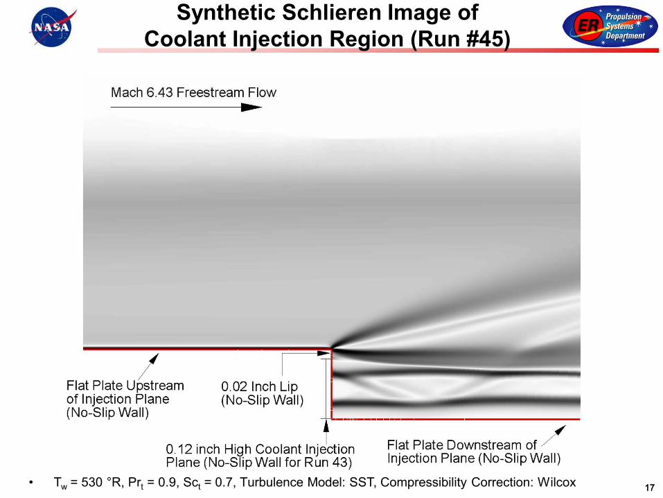
1717
Synthetic Schlieren Image ofCoolant Injection Region (Run #45)
• Tw = 530 °R, Prt = 0.9, Sct = 0.7, Turbulence Model: SST, Compressibility Correction: Wilcox
Mach 6.43 Freestream Flow
•
I Flat Plate Upstream of Injection Plane (No-Slip Wall)
0.02 Inch Lip (No-Slip Wall)
0.12 inch High Coolant Injection Plane (No-Slip Wall for Run 43)
Flat Plate Downstream of / Injection Plane (No-Slip Wall)
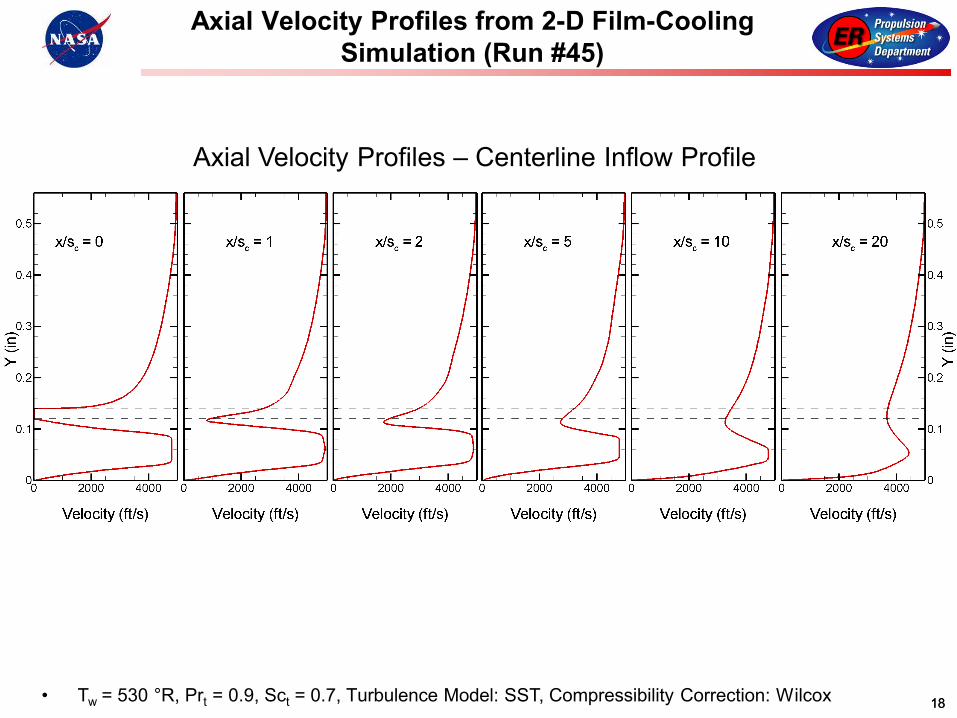
1818
Axial Velocity Profiles – Centerline Inflow Profile
Axial Velocity Profiles from 2-D Film-Cooling Simulation (Run #45)
• Tw = 530 °R, Prt = 0.9, Sct = 0.7, Turbulence Model: SST, Compressibility Correction: Wilcox

1919
Coolant Mass Fraction Profiles – Centerline Inflow Profile
Coolant Mass Fraction Profiles from 2-D Film-Cooling Simulation (Run #45)
• Tw = 530 °R, Prt = 0.9, Sct = 0.7, Turbulence Model: SST, Compressibility Correction: Wilcox
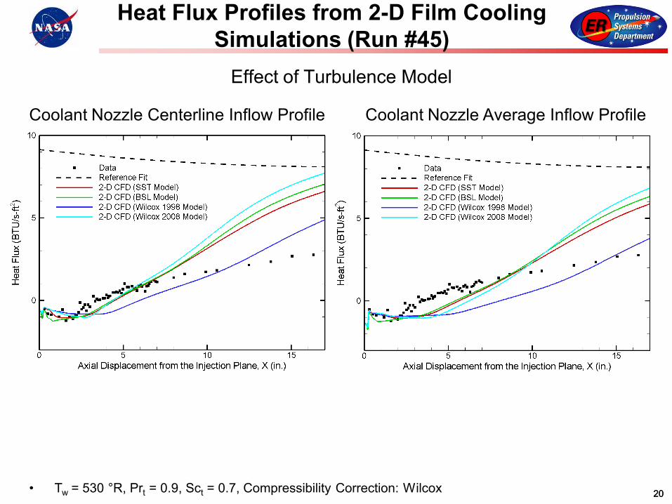
2020
Coolant Nozzle Centerline Inflow Profile Coolant Nozzle Average Inflow Profile
Heat Flux Profiles from 2-D Film Cooling Simulations (Run #45)
• Tw = 530 °R, Prt = 0.9, Sct = 0.7, Compressibility Correction: Wilcox
Effect of Turbulence Model
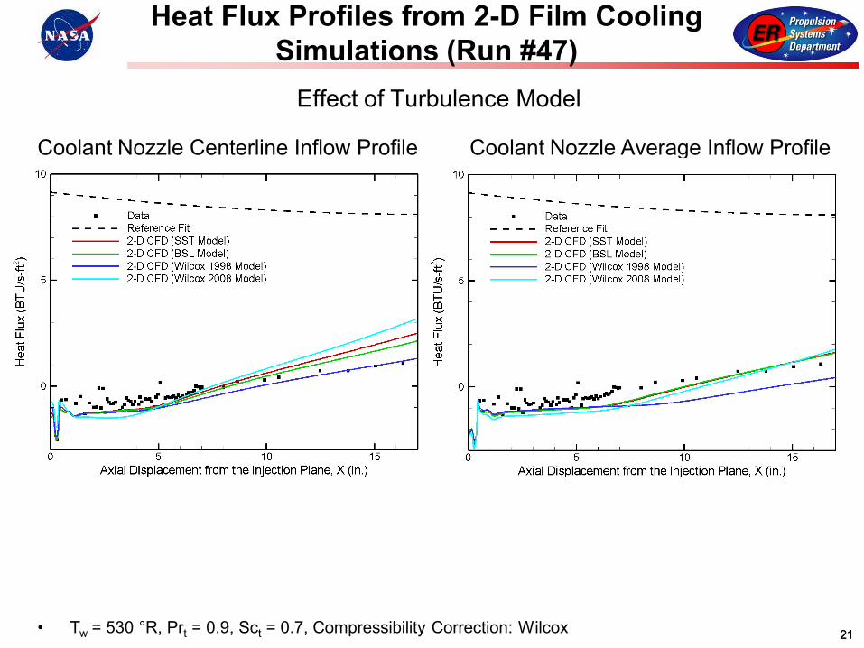
2121
Coolant Nozzle Centerline Inflow Profile Coolant Nozzle Average Inflow Profile
Heat Flux Profiles from 2-D Film Cooling Simulations (Run #47)
• Tw = 530 °R, Prt = 0.9, Sct = 0.7, Compressibility Correction: Wilcox
Effect of Turbulence Model

2222
Coolant Nozzle Centerline Inflow Profile Coolant Nozzle Average Inflow Profile
Heat Flux Profiles from 2-D Film Cooling Simulations (Run #45)
• Tw = 530 °R, Prt = 0.9, Sct = 0.7, Turbulence Model: SST
Effect of Compressibility Correction

2323
Coolant Nozzle Centerline Inflow Profile Coolant Nozzle Average Inflow Profile
Heat Flux Profiles from 2-D Film Cooling Simulations (Run #47)
• Tw = 530 °R, Prt = 0.9, Sct = 0.7, Turbulence Model: SST
Effect of Compressibility Correction

2424
3-D Grid Used for Film Cooling Simulations of Test Article

2525
Heat Flux Contours from 3-D Film-Cooling Simulation (Run #45)
• Tw = 530 °R, Prt = 0.9, Sct = 0.7, Turbulence Model: SST, Compressibility Correction: Wilcox
Heat Flux Contours in Top View (Correct Scale)
Heat Flux Contours in Isometric View (Z Axis Scaled by 10) y
/~,x Heat Flux (BTU/s-ff)
10.0 9.0 8.0 7 .0 6.0 5.0 4.0 3.0 2.0 1.0 0.0
-1 .0 -2.0 -3.0
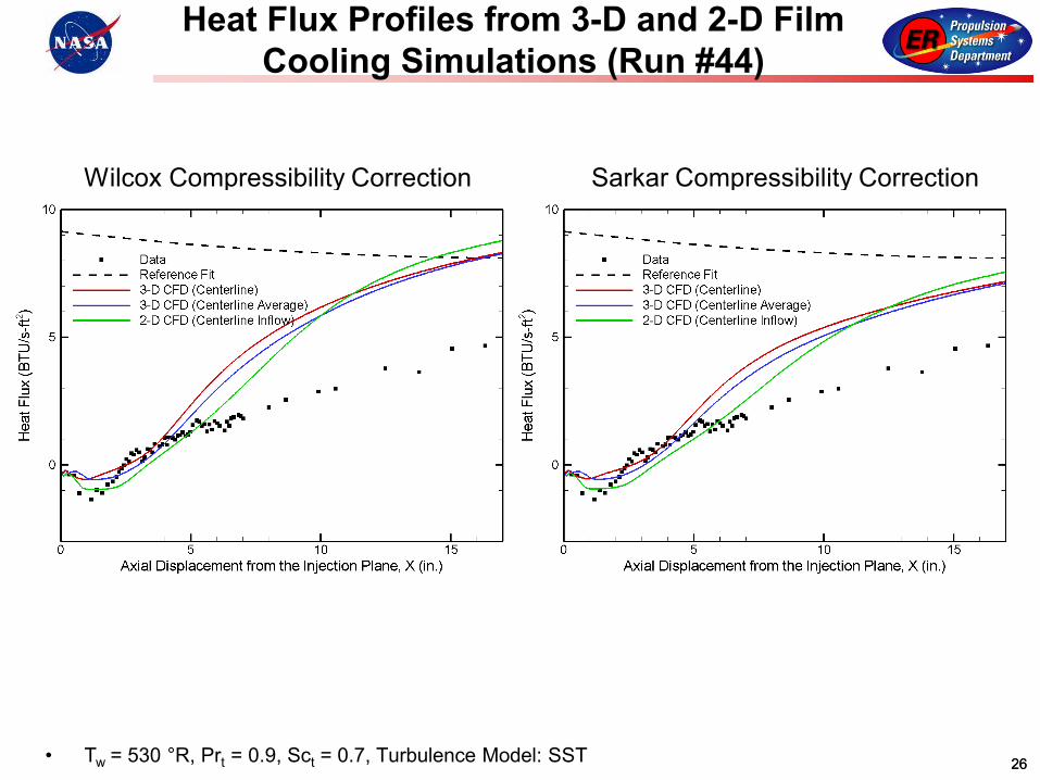
2626
Wilcox Compressibility Correction Sarkar Compressibility Correction
Heat Flux Profiles from 3-D and 2-D Film Cooling Simulations (Run #44)
• Tw = 530 °R, Prt = 0.9, Sct = 0.7, Turbulence Model: SST
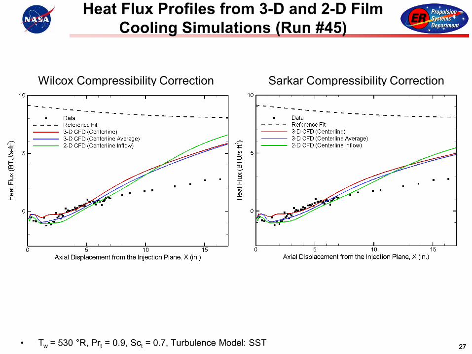
2727
Wilcox Compressibility Correction Sarkar Compressibility Correction
Heat Flux Profiles from 3-D and 2-D Film Cooling Simulations (Run #45)
• Tw = 530 °R, Prt = 0.9, Sct = 0.7, Turbulence Model: SST
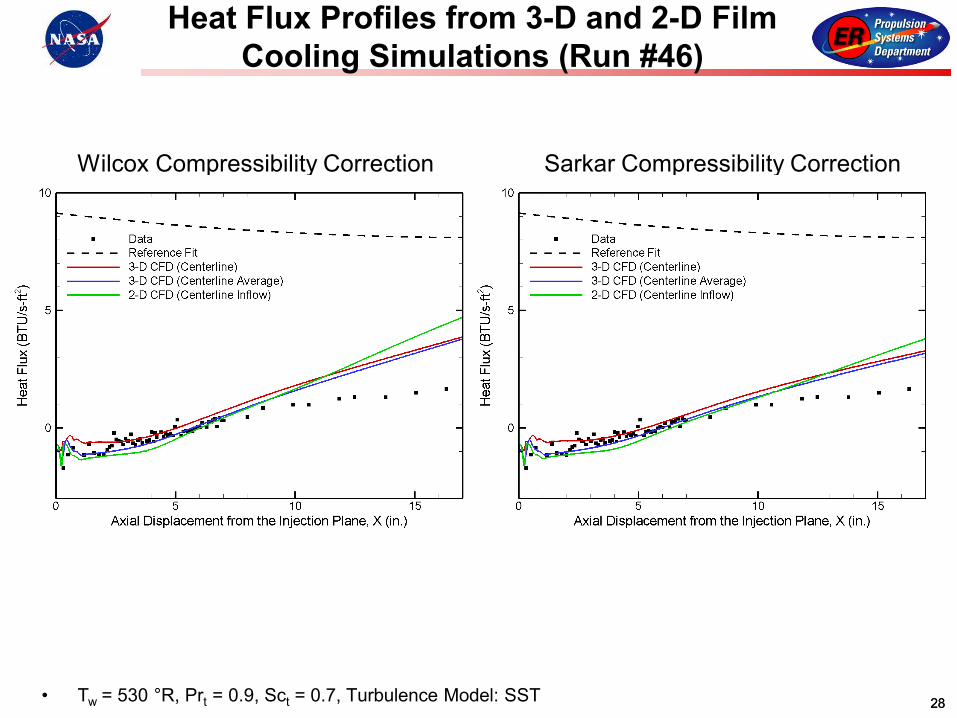
2828
Wilcox Compressibility Correction Sarkar Compressibility Correction
Heat Flux Profiles from 3-D and 2-D Film Cooling Simulations (Run #46)
• Tw = 530 °R, Prt = 0.9, Sct = 0.7, Turbulence Model: SST

2929
Wilcox Compressibility Correction Sarkar Compressibility Correction
Heat Flux Profiles from 3-D and 2-D Film Cooling Simulations (Run #47)
• Tw = 530 °R, Prt = 0.9, Sct = 0.7, Turbulence Model: SST

3030
Summary and Status
Turbulence model compressibility corrections can improve agreement between CFD and the experimental flat plate cases (wall is highly cooled)
3-D simulations of the helium coolant nozzles indicate 3-D viscous effects result in significant flow nonuniformities at the nozzle exit planes
Coolant nozzle mass flow rate is well-predicted by the CFD simulations, but there are unresolved discrepancies with respect to the nozzle exit pressures
Coolant nozzle outflow was approximated as two different profiles for 2-D film-cooling simulations, with mixed results
Compressibility corrections again improve agreement with experimental results 3-D film-cooling simulations indicate significant spanwise variations in heat flux are
present 3-D simulations generally provide a reasonable prediction of the adiabatic cooling
region, but less-good agreement with slope of data in the developed flow region Comparatively large thickness of flat plate boundary layer leads to a wake-like
mixing between the coolant and freestream flows Efforts are underway to resolve knowledge gaps about experiments in consultation
with CUBRC Hydrogen coolant cases have also been run (Ref. NASA TM 4603) and will be
reported in the future