validation of oil trajectory and fate modeling of the

University of Rhode Island University of Rhode Island

DigitalCommons@URI DigitalCommons@URI

Ocean Engineering Faculty Publications Ocean Engineering

2-2021

Validation of Oil Trajectory and Fate Modeling of the Deepwater Validation of Oil Trajectory and Fate Modeling of the Deepwater

Horizon Oil Spill Horizon Oil Spill

Deborah P. French-McCay

Malcolm Spaulding

Deborah Crowley

Daniel Mendelsohn

Jeremy Fontenault

See next page for additional authors

Follow this and additional works at: https://digitalcommons.uri.edu/oce_facpubs

https://digitalcommons.uri.edu/

https://digitalcommons.uri.edu/oce_facpubs

https://digitalcommons.uri.edu/oce

https://digitalcommons.uri.edu/oce_facpubs?utm_source=digitalcommons.uri.edu%2Foce_facpubs%2F32&utm_medium=PDF&utm_campaign=PDFCoverPages

Authors Authors Deborah P. French-McCay, Malcolm Spaulding, Deborah Crowley, Daniel Mendelsohn, Jeremy Fontenault, and Matthew Horn

fmars-08-618463 February 22, 2021 Time: 20:20 # 1

ORIGINAL RESEARCHpublished: 23 February 2021

doi: 10.3389/fmars.2021.618463

Edited by:Robert Hetland,

Texas A&M University, United States

Reviewed by:Thadickal V. Joydas,

King Fahd University of Petroleumand Minerals, Saudi Arabia

Edward Eric Adams,Massachusetts Institute

of Technology, United StatesMatthieu Le Hénaff,

University of Miami, United States

*Correspondence:Deborah P. French-McCay

[email protected]

Specialty section:This article was submitted to

Marine Pollution,a section of the journal

Frontiers in Marine Science

Received: 17 October 2020Accepted: 02 February 2021Published: 23 February 2021

Citation:French-McCay DP, Spaulding ML,

Crowley D, Mendelsohn D,Fontenault J and Horn M (2021)

Validation of Oil Trajectory and FateModeling of the Deepwater HorizonOil Spill. Front. Mar. Sci. 8:618463.

doi: 10.3389/fmars.2021.618463

Validation of Oil Trajectory and FateModeling of the Deepwater HorizonOil SpillDeborah P. French-McCay1* , Malcolm L. Spaulding2, Deborah Crowley1,Daniel Mendelsohn1, Jeremy Fontenault1 and Matthew Horn1

1 RPS, Ocean Science, South Kingstown, RI, United States, 2 Department of Ocean Engineering, University of Rhode Island,Narragansett, RI, United States

Trajectory and fate modeling of the oil released during the Deepwater Horizon blowoutwas performed for April to September of 2010 using a variety of input data sets,including combinations of seven hydrodynamic and four wind models, to determine theinputs leading to the best agreement with observations and to evaluate their reliabilityfor quantifying exposure of marine resources to floating and subsurface oil. Remotesensing (satellite imagery) data were used to estimate the amount and distribution offloating oil over time for comparison with the model’s predictions. The model-predictedlocations and amounts of shoreline oiling were compared to documentation of strandedoil by shoreline assessment teams. Surface floating oil trajectory and distribution waslargely wind driven. However, trajectories varied with the hydrodynamic model usedas input, and was closest to observations when using specific implementations of theHYbrid Coordinate Ocean Model modeled currents that accounted for both offshoreand nearshore currents. Shoreline oiling distributions reflected the paths of the surfaceoil trajectories and were more accurate when westward flows near the MississippiDelta were simulated. The modeled movements and amounts of oil floating over timewere in good agreement with estimates from interpretation of remote sensing data,indicating initial oil droplet distributions and oil transport and fate processes producedoil distribution results reliable for evaluating environmental exposures in the water columnand from floating oil at water surface. The model-estimated daily average water surfacearea affected by floating oil >1.0 g/m2 was 6,720 km2, within the range of uncertainty forthe 11,200 km2 estimate based on remote sensing. Modeled shoreline oiling extendedover 2,600 km from the Apalachicola Bay area of Florida to Terrebonne Bay areaof Louisiana, comparing well to the estimated 2,100 km oiled based on incompleteshoreline surveys.

Keywords: Deepwater Horizon, oil spill model, oil trajectory, oil fate, model validation, deep water blowout, oilexposure, Lagrangian model

INTRODUCTION

Given the catastrophic nature of the Deepwater Horizon (DWH) oil spill of April–July 2010,considerable effort has been applied by many to understand the oil movements and fate, exposureof environmental resources, and potential impacts on biota and ecosystems. Under United Stateslaw, the Natural Resource Damage Assessment (NRDA) was undertaken by the Deepwater Horizon

Frontiers in Marine Science | www.frontiersin.org 1 February 2021 | Volume 8 | Article 618463

https://www.frontiersin.org/journals/marine-science

https://www.frontiersin.org/journals/marine-science#editorial-board

https://www.frontiersin.org/journals/marine-science#editorial-board

https://doi.org/10.3389/fmars.2021.618463

http://creativecommons.org/licenses/by/4.0/

https://doi.org/10.3389/fmars.2021.618463

http://crossmark.crossref.org/dialog/?doi=10.3389/fmars.2021.618463&domain=pdf&date_stamp=2021-02-23

https://www.frontiersin.org/articles/10.3389/fmars.2021.618463/full


https://www.frontiersin.org/

https://www.frontiersin.org/journals/marine-science#articles


French-McCay et al. Deepwater Horizon Oil Spill Trajectories

Natural Resource Damage Assessment Trustee Council (2016)to evaluate exposures to oil and quantify injuries to biota andthe Gulf of Mexico (GOM) ecosystem resulting from the spill,supported by hundreds of studies and thousands of scientists andengineers. As logistics constrained obtaining enough field datato completely characterize the contamination in space and timeduring and after the period of oil and gas release, as part of theNRDA effort in support of the trustees, we pursued a numericalmodeling effort to quantify oil movements, concentrations,exposures of water column biota and biological effects. As afirst step, oil trajectory and fate modeling was performed usingthe established and verified model SIMAP (Spill Impact ModelApplication Package; French McCay, 2003, 2004; French McCayet al., 2015a, 2018b). The results of the oil trajectory and fatemodeling were then used to evaluate exposure and biologicaleffects of fish and invertebrates in the GOM (French McCay et al.,2015a,b,c,d,e). Subsequent to the NRDA settlement in 2016, theoil trajectory and fate modeling was refined as part of modelvalidation studies (French McCay et al., 2018a,c) and pursuantto on-going efforts to evaluate the environmental effects ofthe spill.

The extent of oil contamination from the DWH was visiblyevident during 2010 across the northern GOM in remotesensing imagery (Garcia-Pineda et al., 2013a,b; MacDonald et al.,2015; Svejkovsky et al., 2016) and based on field observations(see review in Deepwater Horizon Natural Resource DamageAssessment Trustee Council, 2016). Oil released from thebroken riser both dispersed at depth and rose through nearlya mile of water column before reaching the surface. Thereare substantial uncertainties in the spill trajectory and spatial-temporal distributions of oil arising from the differences anduncertainties in wind and ocean current model data used toforce the oil spill model, as is evident when comparing publishedoil spill model trajectories (Adcroft et al., 2010; MacFadyenet al., 2011; Liu et al., 2011; Mariano et al., 2011; North et al.,2011, 2015; Dietrich et al., 2012; Paris et al., 2012; Le Heìnaffet al., 2012; Kourafalou and Androulidakis, 2013; Jolliff et al.,2014; Boufadel et al., 2014; Goni et al., 2015; Testa et al.,2016; Özgökmen et al., 2016; Weisberg et al., 2017). Hence,we examined implications of using various wind and currentdata sets, as well as assumptions related to wind drift ofsurface oil, to determine the inputs yielding the most accuratetrajectory for evaluating the oil fate and environmental exposuresresulting from the spill. The trajectories were compared toobservational data such as floating oil distributions based onremote sensing, shoreline oil surveys, chemical analyses of fieldsamples, and sensor data. It is important to consider the influenceof uncertainties in the input data driving transport, as wellas other model inputs, on exposure concentrations relevant toevaluating biological effects.

Thus, the objective of this article was to evaluate the accuracyof DWH model trajectories and oil distributions in the watercolumn and at the surface based on various input data setsand implications to quantification of oil fate and exposureconcentrations. The details of the modeled mass balance,exposure concentrations and biological effects are to be describedin other publications (in preparation).

MATERIALS AND METHODS

ApproachModel simulations were performed using four availablemeteorological and seven hydrodynamic model productscovering the northeastern GOM. In addition, measured currentswere used to evaluate transport along the continental slope.Model trajectories were also performed with winds alone toevaluate the influence of the currents. Wind drift and horizontaldispersion coefficients were altered to evaluate sensitivity tothose assumptions. The model trajectories and concentrationdistributions were compared to observations of surfacingoil, remote sensing data-based observations, shoreline oilingdistributions, fluorescence and other sensor data indicatingthe path of the deep plume, and chemistry sample results. Thefocus of this article is on the influence of physical forcing data(currents and winds) on distributions of surface and shoreline oil.Subsurface oil and oil component concentrations were comparedto field measurement data in French McCay et al. (2018a,c),demonstrating sensitivity to the current data used as input.

Model DescriptionSpill Impact Model Application Package quantifies oilmovements and concentrations of pseudo-componentsrepresenting groups of petroleum compounds of like propertiesin droplet and dissolved phases in the water column, in floatingoil slicks, emulsions and residuals, and as mass stranded onshorelines, settling to sediments, volatilized to the atmosphere,degraded in/on the water, shorelines and sediments, and asremoved by response activities (i.e., mechanical removal andburning). Processes modeled included spreading (gravitationaland by shearing), evaporation of volatile and semi-volatile oilpseudo-components from surface oil, current transport on thesurface and in the water column, randomized dispersion fromsmall-scale motions (mixing), emulsification, entrainment of oilas droplets into the water (natural and facilitated by dispersantapplication), dissolution of soluble and semi-soluble pseudo-components, volatilization of dissolved compounds from thesurface wave-mixed layer, adherence of oil droplets to suspendedparticulate matter (SPM), adsorption of semi-soluble compoundsto SPM, sedimentation, stranding on shorelines, and degradation(using pseudo-component-specific first-order biodegradationand photo-oxidation rates). Sublots of the discharged oil arerepresented by Lagrangian Elements (LEs, called “spillets”), eachcharacterized by location, state (floating, subsurface droplet, onsediment, and ashore), mass of the various pseudo-components,water content of the oil, thickness, diameter (i.e., a floating spillis treated as a flat cylinder with increasing area as oil spreadslocally), density, viscosity, and associated SPM mass. A separateset of LEs is used to track mass, spatial distribution of thediffusing mass, and movements of the dissolved components.

The SIMAP model’s algorithms and assumptions are fullydescribed in French McCay et al. (2018b). The surface oilentrainment algorithm is described in Li et al. (2017a,b).Brief descriptions of the SIMAP oil trajectory and fate model,along with validation studies for two major oil spills, theNorth Cape and the Exxon Valdez oil spills, are available







in French McCay (2003, 2004). Thus, only the most pertinentalgorithms to this reported effort are described here.

Transport is modeled as the sum of advective velocities bycurrents input to the model, wind-driven drift of floating oil,vertical movement of subsurface particles according to (dropletand SPM) buoyancy (using modified Stokes Law; White, 2005),and randomized turbulent diffusive velocities in two (floatingoil) or three (subsurface oil) dimensions (French McCay, 2004;French McCay et al., 2018b). The wind-driven drift due to waves(i.e., Stokes drift) and Ekman transport at the surface was eithermodeled, based on the results of Stokes drift and Ekman transportmodeling by Youssef (1993) and Youssef and Spaulding (1993),which indicates about 3.5% of wind speed 20 degrees to the rightof downwind for a fully developed sea offshore, or assumed aconstant (range 1–4%) of wind speed and either downwind or at aspecified angle. Environmental data such as temperature, salinity,SPM concentrations, water depth, and habitat characteristicswere input as spatial data sets, varying temporally as appropriate(e.g., temperature and salinity).

Another key input influencing oil trajectory is the dropletsize distribution (DSD) of the oil released at depth. The oiland gas from the DWH were released as part of a momentum-dominated jet, which became a buoyant plume (Camilli et al.,2010; Socolofsky et al., 2011, 2015a,b; Johansen et al., 2013;Spaulding et al., 2015, 2017; Gros et al., 2017). As seawaterentrained into the buoyant plume and gas dissolved or escaped,the plume became neutrally buoyant with the surroundingseawater at about 200–400 m above the release point, as wasevident in observational data (Camilli et al., 2010; Diercks et al.,2010; Valentine et al., 2010; Reddy et al., 2012; Spier et al., 2013;Payne and Driskell, 2016, 2017, 2018; Driskell and Payne, 2018).Thus, oil droplets were initialized in the SIMAP model at this“trap height” in droplet sizes estimated by Spaulding et al. (2015;2017; using the Li et al., 2017a algorithm) based on daily estimatesof the oil volume released, the percentage of gas and dispersant(from subsea injection) in the oil and gas plume, the depth ofthe release, the orifice configurations, and the environmentalconditions, all of which are important controlling variables to theDSD (National Academies of Sciences Engineering and Medicine,2020).

Model developments reflected by the DWH analysisherein include the updated oil entrainment algorithm (Liet al., 2017a,b), increased numbers of pseudo-componentstracked (from 7 to 19), refinements in biodegradation andphotolysis rates, the ability to utilize 4-dimentionally varyingenvironmental data sets provided in a variety of grid types,and increased resolution via the numbers of spillets usedand the concentration outputs. The Li et al. (2017a,b) modelallowed the implications of both surface and subsea dispersantapplications on oil droplet size to be addressed. The laterfour developments were needed to address the vast extent ofthe GOM affected, including resolving concentrations over∼2,000 m of water column. Instantaneous, surface spillspreviously addressed (e.g., French McCay, 2003, 2004) hadnot required as much resolution, given that most of theoil was on/in surface waters and many of the componentsevaporated immediately.

Model InputsWindsFour wind reanalysis products covering 2010 in the northeasternGOM obtained from National Oceanic and AtmosphericAdministration (NOAA) and United States Navy governmentwebsites were used as model inputs.

• The North American Mesoscale Forecast System (NAM)data set provided by NOAA National Center forEnvironmental Prediction (NCEP)1 was at approximately12 km resolution and 1-h time steps.• The North American Regional Reanalysis (NARR) data set

provided by NOAA NCEP2 was available at 3-h time stepsand approximately 0.3◦ (32 km) resolution.• The Climate Forecast System Reanalysis (CFSR) data set

provided by NOAA NCEP was a reanalysis of 2010 at ahorizontal resolution of 0.5◦3.• The Navy Operational Global Atmospheric Prediction

System (NOGAPS) data set provided by the United StatesNavy had horizontal resolution of 0.5◦, with a time step of6 h4.

CurrentsCurrent measurements. Acoustic Doppler Current Profiler(ADCP) data meeting quality criteria (French McCay et al.,2018a,c) were available for April–September 2010 from 17locations along the continental slope of the NortheasternGOM (Figure 1). Four ADCPs were deployed near the DWHwellhead site: Development Driller 3 (#42916 at 88.363◦W,28.731◦N sampling 65–1,184 m), Discoverer Enterprise (#42868at 88.356◦W, 28.745◦N sampling 78–1,166 m), and a pair(88.434◦W, 28.742◦N) sampling the upper water column(<100 m) and waters deeper than 1,000 m (1,021–1,501 m) setout by a cooperative NRDA plan on June 18, 2010 (Mulcahy,2010). During the period from April–July 2010, the temporallyaveraged current velocity at station 42,916 was 2.2 cm/s (0.04 kt)to the northeast and 3.9 cm/s (0.08 kt) to the southwest at 64 and1,087 m below the water surface, respectively. The maximumcurrent was 51 cm/s in the surface layer.

The ADCP data meeting quality criteria were used in SIMAPmodel simulations for comparison with simulations run withhydrodynamic model results. The velocity at the location ofeach spillet used for transport calculations at each time step wasinterpolated from the data taken at the 17 ADCP stations usingan inverse distance-weighted scheme employing all sensors. TheADCP coverage extended along the continental slope in the areaof concern, but there were no data on the shelf. In addition,the interpolation provided a smoothed current field, and didnot resolve smaller scale features and shear less than the scaleof the distance between ADCP moorings (order of 30–100 km).

1https://www.ncdc.noaa.gov/data-access/model-data/model-datasets/north-american-mesoscale-forecast-system-nam2http://www.emc.ncep.noaa.gov/mmb/rreanl/3https://www.ncdc.noaa.gov/data-access/model-data/model-datasets/climate-forecast-system-version2-cfsv24https://www.ncdc.noaa.gov/data-access/model-data/model-datasets/navy-operational-global-atmospheric-prediction-system


https://www.ncdc.noaa.gov/data-access/model-data/model-datasets/north-american-mesoscale-forecast-system-nam

https://www.ncdc.noaa.gov/data-access/model-data/model-datasets/north-american-mesoscale-forecast-system-nam

http://www.emc.ncep.noaa.gov/mmb/rreanl/

https://www.ncdc.noaa.gov/data-access/model-data/model-datasets/climate-forecast-system-version2-cfsv2

https://www.ncdc.noaa.gov/data-access/model-data/model-datasets/climate-forecast-system-version2-cfsv2

https://www.ncdc.noaa.gov/data-access/model-data/model-datasets/navy-operational-global-atmospheric-prediction-system

https://www.ncdc.noaa.gov/data-access/model-data/model-datasets/navy-operational-global-atmospheric-prediction-system






FIGURE 1 | Map of the northern Gulf of Mexico region exposed to floating and shoreline oil from the DWH spill, showing 17 ADCP locations. (The DWH wellhead isindicated by the crossed circle. Three ADCP locations are close to the wellhead).

Also, ADCPs do not provide estimates of surface currents. Thus,simulations using ADCPs were realistic only for oil transportbelow the 40 m mixed layer in areas where ADCP data wereavailable, i.e., over the continental slope.

Hydrodynamic models. Seven data sets of currents predicted byhydrodynamic models were evaluated. The wind data from themodel used to force the hydrodynamics, along with the currentdata, was used in the oil spill modeling.

• HYCOM-FSU: Florida State University (FSU) performeda HYbrid Coordinate Ocean Model (HYCOM) hindcastsimulation for 2010 forced with NARR winds. Dataprovided had 3–4 km horizontal resolution, 20 hybridlayers in the vertical, and current predictions every 3 h(Chassignet and Srinivasan, 2015).• HYCOM-NRL Reanalysis: The United States Naval

Research Laboratory’s (NRL) HYCOM + NCODA GOM1/25◦ Reanalysis product GOMu0.04/expt_50.1 for 2010

forced with CFSR winds, ∼3.5 km resolution at mid-latitudes, 36 coordinate surfaces in the vertical, and currentpredictions every 3 h, was downloaded in March 201556.• HYCOM-NRL Real-time: The NRL Real-time operational

forecast GLOBAL HYCOM (Chassignet et al., 2009)simulations for 2010 (HYCOM + NCODA GOM 1/25◦Analysis GOMl0.04/expt_31.0) were forced with NOGAPSwinds. Model resolution is 1/25◦ (∼3.5 km) in thehorizontal, with 20 vertical layers, and hourly data7.• SABGOM: The South Atlantic Bight and Gulf of Mexico

(SABGOM) Regional Ocean Modeling System (ROMS)application was developed by North Carolina StateUniversity (NCSU) for the GOM (Hyun and He, 2010; Xueet al., 2013). The horizontal resolution is ∼5 km with 36

5http://tds.hycom.org/thredds/catalog/datasets/GOMu0.04/expt_50.1/data/netcdf/catalog.html6http://hycom.org/data/gomu0pt04/expt-50pt17https://www.hycom.org/data/goml0pt04/expt-31pt0


http://tds.hycom.org/thredds/catalog/datasets/GOMu0.04/expt_50.1/data/netcdf/catalog.html

http://tds.hycom.org/thredds/catalog/datasets/GOMu0.04/expt_50.1/data/netcdf/catalog.html

http://hycom.org/data/gomu0pt04/expt-50pt1

https://www.hycom.org/data/goml0pt04/expt-31pt0






terrain-following vertical layers. SABGOM was forced withNARR winds. Current predictions were provided every 3 h.• IAS ROMS: The Intra-Americas Sea Regional Ocean

Modeling System (IAS ROMS) was developed fromSABGOM. It was applied with a grid resolution of ∼6 kmin the horizontal and 30 levels in the vertical. An IASROMS simulation (version “4C”) for 2010, that included a2-km nested grid within the larger IAS ROMS domain, wasrun as part of the trustees’ NRDA program and providedby Chao et al. (2014) in April 2014 (model described inChao et al., 2009). This simulation forced with NAM windsprovided hourly data.• NCOM Real Time: The Naval Oceanographic Office

(NAVOCEANO) ran the three-dimensional operationalglobal nowcast/forecast system Global NCOM through2013. NCOM was based on the Princeton Ocean Model(POM) with time invariant hybrid (sigma over Z)vertical coordinates with 40 levels8. Predictions wereprovided every 3 h.• NGOM: The NOAA National Ocean Service (NOAA/NOS)

Coast Survey Development Laboratory (CSDL) ran theNOS GOM Nowcast/Forecast Model (NGOM), a GOMimplementation of the POM, in real time during thespill, forced by NAM winds. The resolution is 5–6 km inthe northeastern and central GOM, with 37 levels in thevertical. Predictions were provided every 3 h.

Geographical dataA rectilinear grid was used to designate the location of theshoreline, the water depths (bathymetry), and the habitat or shoretypes. NOAA Office of Response and Restoration, EnvironmentalSensitivity Index data9 were used to define shoreline habitat types,reclassifying Environmental Sensitivity Index codes to a simplerhabitat classification, i.e., rocky, cobble, sand, mud, wetland,and artificial (man-made) shore types. Bathymetric data wereobtained from the General Bathymetric Chart of the OceansDigital Atlas (General Bathymetric Chart of the Oceans, 2009)one arc-minute gridded data set, which is based on quality-controlled ship depth soundings interpolated using satellite-derived gravity data as a guide.

Oil loading onto shorelines was assumed to occur up to amaximum holding capacity that was related to shore type (andso shoreline wave climate, slope, width, and grain size) and thebeaching oil’s viscosity. Shore holding capacities as a functionof oil viscosity were developed for each shore type based onobservations from the Amoco Cadiz spill in France and theExxon Valdez spill in Alaska, as described in French et al. (1996)and French McCay et al. (2018c).

Environmental conditionsIn order to utilize the same temperature and salinity distributionsfor all model runs, and given the uncertainties in the subseadistributions and currents predicted by the hydrodynamicmodels, monthly mean water temperature and salinity data fromthe World Ocean Atlas (Boyer et al., 2004) were input on a

8http://ecowatch.ncddc.noaa.gov/global-ncom/9http://response.restoration.noaa.gov/esi

three-dimensional grid. The floating oil model trajectory was notsensitive to the difference in resolution between the atlas dataand the hydrodynamic model data, since most of the oil surfacedwithin hours of release. A synoptic map of SPM concentrationswas defined for use in the oil spill modeling by combining resultsfrom field and modeling studies with satellite imagery depictingSPM plumes (French McCay et al., 2018a,c).

For the base cases, the horizontal diffusion (randomizedturbulent diffusion) coefficient was assumed 100 m2/s for floatingoil, 2 m2/s in surface waters (above 40 m), and 0.1 m2/s inwaters below 40 m. The vertical diffusion coefficient was assumed10 cm2/s in surface and 1–0.1 cm2/s in deep waters. Thecoefficients were also varied in sensitivity analyses up to oneorder of magnitude larger and smaller. These values are based onempirical data reviewed for the deep-water GOM (French McCayet al., 2015a; based on Okubo and Ozmidov, 1970; Okubo, 1971,Csanady, 1973; Socolofsky and Jirka, 2005, Ledwell et al., 2016).

Oil properties, composition, and degradationThe spilled oil was a light GOM crude oil. The liquid “dead” oil(i.e., oil without the C1 to C4 natural gas hydrocarbons) densitiesat 5, 15, and 30◦C were 0.8560, 0.8483, and 0.8372 g/cm3,respectively; dynamic viscosity was 10.93 cp at 5◦C, 7.145 cp at15◦C, and 4.503 cp at 30◦C; and IFT was 19.63 mN/m (Stout,2015b). Based on its asphaltene (0.27%) and resin (10.1%) content(in un-weathered dead oil, Stout, 2015b) and behavior of similarlight crude oils (Fingas and Fieldhouse, 2012), the fresh oilwould form an unstable emulsion. After weathering concentratedasphaltenes and resins sufficiently, the oil was observed andassumed to form a mesostable water-in-oil emulsion (mousse) upto a maximum water content of 64% water (Belore et al., 2011).

Concentrations of volatile-insoluble and soluble to semi-soluble hydrocarbons and related compounds were calculatedfor 18 pseudo-components used to characterize the dead oil[including nine soluble/semi-soluble and volatile/semi-volatilecomponents defined by octanol-water partition coefficient(Kow) range, eight insoluble and volatile/semi-volatile aliphaticcomponents defined by boiling ranges, and one residual oilcomponent; French McCay et al., 2015a, 2018b] and input to theSIMAP oil fates model, along with fractions of the oil volatilizedin boiling cut temperature ranges (Stout, 2015a; Stout et al.,2016a). Physical-chemical properties of each pseudo-componentwere developed by French McCay et al. (2015a).

First-order biodegradation rates in the water column usedas model input were based on reviews by French McCay et al.(2015a, 2018a,b) to develop pseudo-component-specific rates.Photo-oxidation rates of polycyclic aromatic compounds byultraviolet light were developed by French McCay et al. (2018d).

Amounts and droplet sizes of released oilThe DWH spill location (88.367◦W, 28.740◦N in MississippiCanyon Block 252, MC252; Figure 1) was ∼80 km southeast ofthe mouth of the Mississippi River in ∼1,500 m of water. Theamount of oil (C5+) released to the environment (totaling 4.1million bbl, ∼554 thousand metric tons, MT; i.e., not includingthe amount recovered at the release site) was specified fromApril 22, 2010 at 10:30AM CDT (local time) for 2015 hours (i.e.,


http://ecowatch.ncddc.noaa.gov/global-ncom/

http://response.restoration.noaa.gov/esi






84 days until July 15, 2010 at 2:30PM CDT) in 15-min time-stepincrements using daily estimates based on information providedby the Flow Rate Technical Group (McNutt et al., 2011, 2012),as summarized by Lehr et al. (2010). The oil mass was initializedin the SIMAP model at depths and in DSDs calculated via thenearfield and droplet size models, reflecting subsea dispersantapplication activities (Li et al., 2017a; Spaulding et al., 2017).

From April 28 to June 3, oil and gas flowed from both thebroken end of the fallen riser and holes in a kink in the riserpipe just above the blowout preventor. After June 3 (when thefallen riser pipe section was sawed off and Top Hat #4 with arecovery pipe was placed over the riser), oil was released onlyfrom the riser pipe, around the top hat immediately above theblowout preventor. The median droplet diameters of the riserflows (∼2–3 mm) were significantly larger than those fromthe kink release (∼300–500 µm), due to the much higher exitvelocity from the kink relative to the larger diameter riser release.For most model simulations, the best estimate of the DSDwas used, which was a bimodal distribution based on partialdispersant treatment of the oil in the blowout plume (detailsin Spaulding et al., 2015, 2017). Sensitivity to the boundingrange DSDs resulting from assumed high (100%) and low (50%)effectiveness of the subsea dispersant injections (Spaulding et al.,2015, 2017) was examined for simulations using HYCOM-FSU.

Response activitiesModeled response activities at the water surface included removalby in situ burning and dispersant application to floating oil fromthe air and vessels. Spatially explicit quantitative measurements ofoil volume mechanically removed were not available; therefore,mechanical cleanup was not included in the model simulations.Polygons were input to the model specifying amounts of oilburned or treated by dispersant, and where and when theresponse activities occurred. Details are provided in FrenchMcCay et al. (2018c).

Quantitative estimates of oil volume removed by in situburning were obtained from the Response After-Action Reportby Mabile and Allen (2010; summarized by Lehr et al., 2010; Allenet al., 2011). Time ranges for burns each day were compositedinto a daily burn time window. The mass rate of removal on agiven date was calculated as the total burn volume times typicalfloating oil density in the areas of the burns, 0.97 g/cm3, dividedby the time range of burning that day. The model removed oilmass at this daily rate within each time and spatial window up tothe maximum daily mass prescribed by the model input.

Surface dispersant application data were obtained fromresponse records (NOAA, 2013). The volume of oil treated perdispersant volume applied (i.e., the dispersant-to-oil ratio) wasbased on assumptions in Lehr et al. (2010), who assumed thatthe minimum, median, and maximum ratios were 5, 10, and 20by weight of oil, not including the water in mousse. The medianvalue (1:10) was used as the base case. The fraction of oil dispersedinto the water column (i.e., efficiency) was calculated using theentrainment algorithm (Li et al., 2017b) based on the assumeddispersant-to-oil ratio and resulting interfacial tension (based ondata from Venkataraman et al., 2013).

Analysis of ResultsTo evaluate model agreement with observations, modeledfloating oil distributions were compared to interpretations ofremote sensing imagery, modeled shoreline oiling was comparedto field survey data, and modeled subsea concentrations werecompared to chemistry sample data and sensor-based indicators(e.g., fluorescence peaks).

Floating OilRemote sensing (satellite) imagery data were used to evaluatethe distributions of surface oil over time. Remote sensinginterpretations, developed as part of the trustees’ NRDA programin support of the Deepwater PDARP/PEIS (Deepwater HorizonNatural Resource Damage Assessment Trustee Council, 2016)for April to August 2010 were downloaded from the NOAAGOM ERMA website (http://gomex.erma.noaa.gov/erma.html)on January 27, 2016 (ERMA, 2016). Data from four sensorswere available: Satellite Synthetic Aperture Radar (SAR), MODISVisible, MODIS Thermal IR Sensor data (MTIR), and LandsatThematic Mapper (TM).

Synthetic Aperture Radar images were analyzed for presenceand thickness category (thick or thin) of floating oil by DeepwaterHorizon Natural Resource Damage Assessment Trustee Council(2016; based on Garcia-Pineda et al., 2009, 2010, 2013a,b;Graettinger et al., 2015). MacDonald et al. (2015) used a neuralnetwork analysis of SAR images to quantify the magnitude(averaging 70 µm for thick and 1 µm for thin) and distributionof surface oil in the GOM from persistent, natural seeps and fromthe DWH discharge. SAR resolutions ranged from 25 to 100 mper pixel, with a few images at 6 m per pixel (Graettinger et al.,2015; ERMA, 2016).

MODIS Visible data were available for 18 days depictingsurface oil, at a pixel resolution of 250 or 500 m, depending on thespectral band. The images were classified into three oil thicknessclasses: thin oil class (primarily silver sheen and rainbow, usingNOAA, 2016), a thick oil class (transitional dark to dark color),and a moderately thick oil class (metallic sheen) that falls betweenthe other two classes (Graettinger et al., 2015; ERMA, 2016).

MODIS Thermal IR data at a pixel resolution of 1,000 m wereavailable for 25 days during the spill period. The images wereclassified into a thin oil class [primarily silver sheen and rainbow,using NOAA (2016) nomenclature], a thick oil class (transitionaldark to dark color), and a moderately thick oil class that fallsbetween the other two classes (Graettinger et al., 2015; ERMA,2016).

Useful Landsat TM data were available over a spatially limitedarea on 8 days when DWH oil was on the surface of the northernGOM. Landsat TM satellite data have a pixel resolution of about30 m. Ocean Imaging estimated the areal coverage per pixel ofthree oil thickness classes: a very thick class comprising heavyemulsions, a moderately thick class of dark/opaque oil, and athin oil category that is thicker than sheen but thinner thandark/opaque oil. The Landsat TM oil thickness analyses did notclassify oil sheens (Graettinger et al., 2015; ERMA, 2016).

For comparisons with model results, floating oil distributionsfrom 84 dates and times were used, these being times wherethe image was judged sufficiently synoptic of the area of the


http://gomex.erma.noaa.gov/erma.html






floating oil. These included 34 SAR, 18 MODIS Visible, 25MODIS Thermal IR, and 7 Landsat TM images (SupplementaryTable 1). The three thickness classes of the MODIS Visible,MODIS Thermal IR, and Landsat TM images were assumed 1,10, and 50 µm thick on average, based on ranges estimated byGraettinger et al. (2015). Graettinger et al. (2015) and MacDonaldet al. (2015) aggregated the pixelated data as gridded data in a5 × 5 km2 geographic grid and developed statistical models tointerpolate between observations in space and time. However,since the interpolations may have missed weather-related andother events between actual observations, comparisons of theSIMAP model results to imagery results were made using thepixelated data based on the observational data, without use ofthe interpolations. These non-interpolated data were gridded inthe same 5 km by 5 km grid used by the Deepwater HorizonNatural Resource Damage Assessment Trustee Council (2016;Graettinger et al., 2015; ERMA, 2016).

For both the remote sensing data and the model, at eachobservation time for the remote sensing, the percentage offloating oil present in each grid cell was calculated in three ways.

• The relative area of oil in each grid cell indicated thedistribution of oil cover. For remote sensing data, the areawithin the cell covered by oil was divided by the total areaof oil in all cells estimated from the imagery. For the model,the area covered by spillets falling in the cell was dividedby the total area covered by all floating spillets at thattime step (accounting for overlapping spillet areas, avoidingdouble-counting).• The estimated volume of oil in each grid cell was calculated

for remote sensing data from the area covered by eachthickness category. For the model, the total mass in spilletsfalling in the cell was used as an index of volume.• The relative volume of oil in each grid cell accounts for

the relative distribution of oil, irrespective of the actualamounts, which are subject to the assigned oil thickness.For remote sensing data, the volume of oil in each cell wasdivided by the total volume of oil in all cells estimated fromthe imagery. For the model, the total mass in spillets fallingin the cell was divided by the total mass of all floating spilletsin all cells at that time step. The mass was not correctedfor oil density to convert to volume. Thus, all spillets wereassumed to be of equal density for this index.

The Root Mean Square Error (RMSE) was calculated foreach date/time there was an observation available. The RMSEis a frequently used measure of the differences between valuespredicted by a model and the values observed, and thus isa measure of accuracy. The individual differences (residuals)are aggregated in the RMSE as a single measure of predictivepower (Fitzpatrick, 2009). For each pair of grids, the RMSE wascalculated by summing the squares of the differences betweenmodeled and the observed over all cells of the grid, where n = totalnumber of cells in each grid:

RMSE =

√∑(observed −modeled

)2

n

RMSE values were averaged over all dates, in order to judgerelative fit comparing dates and/or among simulations, theminimum RMSE indicating the best fit.

Shoreline Oil DistributionsAvailable data for shore oiling consisted of maps of where oil wasfirst observed on various shoreline segments and assessments bythe Shoreline Cleanup and Assessment (SCAT) program duringResponse. A binary discriminator test (Fitzpatrick, 2009) wasused to evaluate the timing of oil coming ashore in the model,as compared with observations made by the SCAT program. Thepresence or absence of oil according to SCAT observations andthe model predictions were gridded using the 5 km by 5 kmAlbers grid (ERMA, 2016) employed by the Deepwater HorizonNatural Resource Damage Assessment Trustee Council (2016) intheir evaluations of oil exposure after the DWH spill. A cell wasconsidered to have oil presence if any shore segment within thecell was observed oiled by the SCAT teams.

SCAT data were downloaded from ERMA in July of 2014 asshape files10. The observational data were binned into 10-dayintervals, from April 22 to September 30, 2010. In the analysis,only those SCAT segments where oil was observed to arrivebefore September 30 were considered as oiled. Segments checkedduring the 10-day interval, but where no oil was observed toarrive, were considered as “no oil.” Segments where oil wasobserved to arrive after September 30, but earlier observationsshowed it did not arrive there before September 30, were coded as“no oil.” Note that the shorelines were not searched synoptically,and areas were not visited for days or weeks; thus, the time oil wasfirst observed could have been a considerable time after the actualinitial oiling. Also, the Deepwater Horizon Natural ResourceDamage Assessment Trustee Council (2016) used additionalobservations and SAR to identify where oil came ashore, todevelop more comprehensive maps of the locations where oilcame ashore during and after (including after September 30) thespill. However, we relied solely on the SCAT survey data, as theSAR-based data were localized analyses at specific instances.

Subsea OilModeled subsea concentrations were compared to chemistrysample data and sensor-based indicators (e.g., fluorescencepeaks) both qualitatively, to evaluate oil locations, andquantitatively, to evaluate concentrations. We used chemicalmeasurements of samples taken May 11 (the first date available) –July 15, 2010 and processed by the trustees’ quality-controlledNRDA program (Deepwater Horizon Natural Resource DamageAssessment Trustee Council, 2016; described in Horn et al.,2015; Payne and Driskell, 2015b, 2016, 2017, 2018; Driskelland Payne, 2018). The NRDA sample data set is available inERMA (2016). Details of the model comparisons to subseachemistry data are in French McCay et al. (2015a, 2018a). Wesummarize those findings below as part of the present analysisof the influence of physical forcing on the model trajectories andoil distributions.

10http://gomex.erma.noaa.gov/erma.html


http://gomex.erma.noaa.gov/erma.html






RESULTS AND DISCUSSION

The model trajectory selected as the base case for waters above200 m was that forced with the hydrodynamic and wind inputcombination (i.e., HYCOM-FSU currents and NARR winds)yielding the best agreement with floating oil distributions andshoreline oiling over time. In deep water, ADCP data yielded thebest agreement with oil contaminant distributions >200 m anddefining the deep plume. Videos of the floating oil movementscolor-coded by “age” (time since release) and of the oil droplettrajectory below 900 m are in Supplementary Material.

Floating OilIn prior modeling examining mass balance and fate of oil releasedfrom hypothetical oil and gas blowouts in nearby locations of theGOM (French McCay et al., 2018d, 2019), the initial DSD was themost influential input controlling the amount of oil surfacing. Fora spill at 1,400 m, with a trap height at 1,100 m (i.e., similar to theDWH spill), a DSD with a median droplet size <700 µm reducedthe amount of surfacing oil dramatically, whereas the amount ofoil surfacing was similar for all DSDs with larger median dropletsizes (French McCay et al., 2019). As the breadth of (range ofdroplet sizes in) the DSD has been found to be narrow (Li et al.,2017a), most of the mass in the DSD is in droplet sizes close tothe median droplet diameter.

In all model simulations, oil droplets >0.7 mm diameter,weathered by dissolution such that their density when theyreached the surface approached 940 kg/m3 (in agreement withmeasurements of “fresh” floating oil by Stout et al., 2016a), roseto the surface in <17 h. Droplets 1 and 3 mm in diametersurfaced in 11 and 3 h, respectively. ADCP-measured currentsat the wellhead averaged <5 cm/s between 40 and 1,400 m.Assuming a mean current of 5 cm/s during their rise, 0. 7-, 1-,and 3-mm droplets would travel ∼2, 3 and 0.5 km horizontally,respectively. Svejkovsky and Hess (2012); Svejkovsky et al. (2016)and Payne and Driskell (2015d, 2018) observed fresh oil surfacing<4 km from the wellhead on various dates in May and June 2010.Ryerson et al. (2012) observed fresh (as evidenced by measuredvolatiles in the air above) oil surfacing at 1.0 ± 0.5 km from thewellhead June 8–10, 2010, which based on ADCP measurementsat that time implied a 10-h surfacing time. Ryerson et al. (2012)noted that visual observations from response vessels suggested a∼3-h lag time between deliberate intervention at the well and theonset of changes in the freshly surfaced oil. These observationsimply that much of the surfaced oil was comprised of droplets∼1–3 mm in diameter. Droplets smaller than 0.7 mm roseover a longer period and so were carried progressively fartherfrom the release point. Droplets less than ∼100 µm did notrise appreciably and formed the deep-water plume along withdissolved hydrocarbons. Thus, the DSD could affect the surfacinglocations of the oil, and the floating oil distribution, dependingon the relative amounts of mass in these size ranges. Floating oilwould be more spread out from the well if most of the mass wasin droplet sizes <700 µm than it would be if most of the masswere in droplets >700 µm.

Figure 2 shows the cumulative days of oil presenceon the water surface based on SAR analysis (data from

ERMA, 2016, produced by Graettinger et al., 2015). Figure 3and Supplementary Figures 1–10 summarize the oiled footprints(north of 27◦N and east of 92◦W, the domain used forcomparisons to focus on most of the oil and limit the numberof null cells) for the model trajectories forced by various windsand currents as cumulative days of oil presence on the watersurface in each grid cell over the simulation. The average RSMEvalues over all dates of comparison for these runs, assumingthe floating oil horizontal dispersion coefficient was 100 m2/sand using the modeled wind drift, are in Table 1. For the basecase using HYCOM-FSU and NARR winds, and all simulationsusing other hydrodynamics, the DSD was the best estimate, asdescribed in Spaulding et al. (2015, 2017). High and low cases inTable 1 represent the potential range of DSDs (Spaulding et al.,2015, 2017).

Considering the RSME means for all three metrics, thebase case using HYCOM-FSU with NARR winds produced atrajectory that best fit the remote sensing data. IAS ROMSshowed second best agreement to the remote sensing in termsof the relative spatial distribution of floating oil (relative areaand relative volume). However, the HYCOM-NRL Reanalysiswith CFSR winds showed the same degree of agreement withthe remote-sensing data as the HYCOM_FSU/NARR simulationin terms of oil volume distribution (Table 1). SABGOM movedmore oil northeast toward Florida in June than did the otherhydrodynamics (Supplementary Figure 3). The HYCOM-NRLReal-time hydrodynamics transported more oil southeast towardsouthern Florida (Supplementary Figure 2) than was observedin the remote sensing (Figure 2). The RMSE values show pooreragreement of the model with the remote sensing products whenno currents and only winds are used, than for when any ofthe hydrodynamic models are used (Table 1), indicating thatthe hydrodynamic model currents improved the trajectoriesover wind drift alone. Use of ADCP data for surface transport(extrapolated from below 40 m) resulted in better agreementto the observational data than without currents, suggestingthat transport of droplets rising from depth, and thus theDSD, influenced the floating oil distribution. While the mappedcomparison (Supplementary Figure 7) showed the floating oildistribution reasonably agreed with the observations, there wasno ADCP data on the shelf or nearshore, such that along-shoretransport was not captured and there was not enough eastwardor westward spread of the oil. Thus, the simulations usinghydrodynamic modeled currents produced better agreement withthe observed floating oil distributions than simulations usingADCP data for currents. However, as will be discussed in section“Subsea Oil,” modeled oil distributions below 40 m were in betteragreement with ADCP-based observational data than simulationsusing any of the hydrodynamic models.

Across the range of potential subsea dispersant effectivenessassumptions (high and low cases in Table 1), the DSDs influencedthe volume distribution of the floating oil to a similar degree asvarying the hydrodynamic model input. However, the relativearea and relative volume RMSE values did not change much withchange in DSD within the potential range (Spaulding et al., 2015,2017), whereas those metrics were sensitive to the hydrodynamicinput. The best-estimate DSD used for the base case with







FIGURE 2 | Cumulative days of oil presence on the water surface, based on remote sensing (SAR) analysis (data from ERMA, 2016).

HYCOM-FSU yielded the lowest RMSEs overall (Table 1). Thus,the floating oil spatial and volume distributions were sensitive tothe hydrodynamics used. The relative spatial distribution of thefloating oil was not sensitive to the plausible DSD inputs becausethe substantial mass in large droplets (>0.7 mm) surfaced closeto the well and resulted in similar trajectories, regardless of theamount in those droplet sizes. If the DSD were skewed to muchsmaller sizes than those examined, the relative spatial distributionwould be affected, and floating oil would be more broadlydistributed since smaller droplets would be carried farther fromthe well before surfacing. However, such DSDs are not realisticfor the DWH spill where the conditions and dispersant volumesapplied at depth were not conducive to creating smaller dropletsizes (Adams et al., 2013; Zhao et al., 2014, 2015; Socolofskyet al., 2015b; Spaulding et al., 2015, 2017; Nissanka and Yapa,2016; Testa et al., 2016; Gros et al., 2017; Li et al., 2017a; Daaeet al., 2018; National Academies of Sciences Engineering andMedicine, 2020). The extremely low estimates of the median(<100 µm) and maximum (<300 µm) droplet diameters (forboth untreated and treated oil) of Paris et al. (2012) and Amanet al. (2015) were not representative of the DWH conditions (see

Adams et al., 2013; Testa et al., 2016), nor are they consistent withthe field evidence.

As SIMAP is a Lagrangian model, the diffusion coefficientsmoved the spillet centers randomly each time step at a scaledetermined by the coefficient. Those displacement distanceswere small relative to the ∼5-km concentration grid used tocompare the model to the remote sensing data. Thus, theRMSE values changed slightly (<10%) with differing floating oilhorizontal dispersion coefficients from 5 to 200 m2/s, indicatingthis assumption had little influence on the results at the scaleof a 5 km grid. The hydrodynamic models did not resolvethe surface oil drift in the upper wave-mixed layer resultingfrom wave motions and Ekman flow. Simulations using theYoussef and Spaulding (1993) model of these processes, aswell as varying percentages-of-wind-speed drift rates (2–4%)and angles (0–20◦) to the right of downwind, showed that thebest fit was consistently that using the Youssef and Spaulding(1993, 1994) model, as opposed to using a constant wind driftpercentage and angle for all dates, although the differencesbetween the results were small on most days (results notshown). Moreover, there was much more variation between







FIGURE 3 | Cumulative days of oil presence on the water surface, based on the base case model simulation using HYCOM-FSU currents and NARR winds.

runs with different currents and winds used for forcing thanthe differences due to variation in wind drift model or thehorizontal dispersion coefficient. Thus, variations of wind driftand horizontal dispersion coefficient assumptions were notexamined further. Use of 800,000 spillets instead of 100,000spillets (as used for the simulations presented) to representthe floating oil slightly improved the model agreement withthe observed for the HYCOM-FSU base case, as the additionalspillets filled in some of the areas where remote sensing dataindicated oil was present. However, model run time was increasedconsiderably in the tests using more spillets.

Snapshots of surface oil distributions over time, predicted bythe model using HYCOM-FSU currents and based on remotesensing data, are compared in the Supplementary Material.Comparative snapshots for other model simulations are availablein French McCay et al. (2018c). Figure 3 and SupplementaryFigures 1–10 summarize the trajectories and comparisons. Theremote sensing data indicate the floating oil was primarily ina circular area near and just north of the DWH wellhead.The simulations using HYCOM-FSU (Figure 3), HYCOM-NRL Reanalysis (Supplementary Figure 1), and IAS ROMS

(Supplementary Figure 6) show similar patterns. The resultsof the simulations with other currents show excursions too farnortheast (SABGOM, Supplementary Figure 3; NCOM Real-time, Supplementary Figure 4), and too much dispersion in alldirections (HYCOM-NRL Real-time, Supplementary Figure 2;NGOM, Supplementary Figure 5). The three simulationsusing no currents and NAM, NARR or NOGAPS winds(Supplementary Figures 8–10) are similar, and do not transportof the floating oil enough to the east or west. Otherwise, theno-current simulations result in realistic floating oil patternscentered just north of the wellhead. The simulation using ADCPcurrents and NARR winds generates results similar to no currentsand NARR winds (Supplementary Figure 7), because the ADCPcurrents are relatively weak in the offshore area and do not coverthe shelf or nearshore. These results indicate the importance ofthe wind drift in transporting the floating oil, but that the currentsused can change the patterns dramatically.

The modeled number of days of oil cover for the base caseusing HYCOM-FSU (Figure 3) is of the same range as the SAR-based estimates (Figure 2) in the area of the wellhead and off theMississippi River Delta. However, the duration of oil cover in the







TABLE 1 | RMSE (mean over all dates) comparing modeled to remote sensingdata for floating oil distributions, varying currents and winds used as input.

Currents Winds RMSE:relative

area

RMSE:relativevolume

RMSE:volume (m3)

HYCOM-FSU (base case) NARR 0.00053 0.00082 17.3

HYCOM-FSU (high) NARR 0.00052 0.00080 17.7

HYCOM-FSU (low) NARR 0.00054 0.00083 19.6

SABGOM NARR 0.00057 0.00090 21.2

HYCOM-NRL Reanalysis CFSR 0.00061 0.00100 17.3

HYCOM-NRL Real-time NARR 0.00058 0.00088 19.4

NCOM Real-time NARR 0.00060 0.00090 21.3

NGOM-NOAA Real-time NARR 0.00059 0.00088 19.1

IAS ROMS NAM 0.00056 0.00087 19.7

ADCP NARR 0.00068 0.00107 21.6

None NAM 0.00070 0.00104 22.9

None NARR 0.00072 0.00109 25.3

None NOGAPS 0.00075 0.00112 25.5

For all model simulations except those noted as high or low, the best estimate ofthe droplet size distribution was used. High and low represent the range of potentialdroplet size distributions by varying subsea dispersant effectiveness from high tolow (Relative area and relative volume are unitless).

area near the coast of Mississippi and Alabama is higher in themodel than the SAR data indicate. Also, floating oil trapped nearshore in the model remained longer than observed. Mechanicalremoval, on water or on shorelines, was not included in thesimulations, and this could potentially account for at least someof the observed reduction in the nearshore floating oil.

The RMSE values for the base case using HYCOM-FSUcurrents (Figure 4) show the best agreement in terms of relativearea or relative volume distribution in early June, whereasthe model estimated volume of oil was most similar to theremote-sensing based estimates in April-early May and inJuly. The results for other current-wind combinations showedsimilar temporal patterns. The relatively high RMSE values forspatial coverage in April were because the modeled distributionremained more localized around the wellhead than the remotesensing indicated. The relatively high RMSE value for relativevolume on May 17 was for the MODIS visual image of that date,when the “Tiger Tail” feature (i.e., the extension to the southeastas oil sheen was drawn into a cyclonic eddy) was seen in theimagery (Walker et al., 2011; Olascoaga and Haller, 2012) butnot indicated by the model (i.e., the hydrodynamic model did notlocate the eddy in the same location at that time).

The modeled maximum amount of oil in each grid cell atany time in the simulation is shown in Figure 5. Using griddingwith a cell size of 25 km2, MacDonald et al. (2015) estimatedthe footprint of aggregated floating oil and oil emulsions, whereoil coverage exceeded ∼1 g/m2 at some time during the spill,which extended over 149,000 km2. By comparison, the basecase model prediction, using the same resolution and threshold,was 194,000 km2. The model predictions included some lowconcentrations of floating oil in areas far from the well whereoil was not detected by the remote sensing. These small patchesof highly weathered oil residuals (>20 days old) in the outskirts

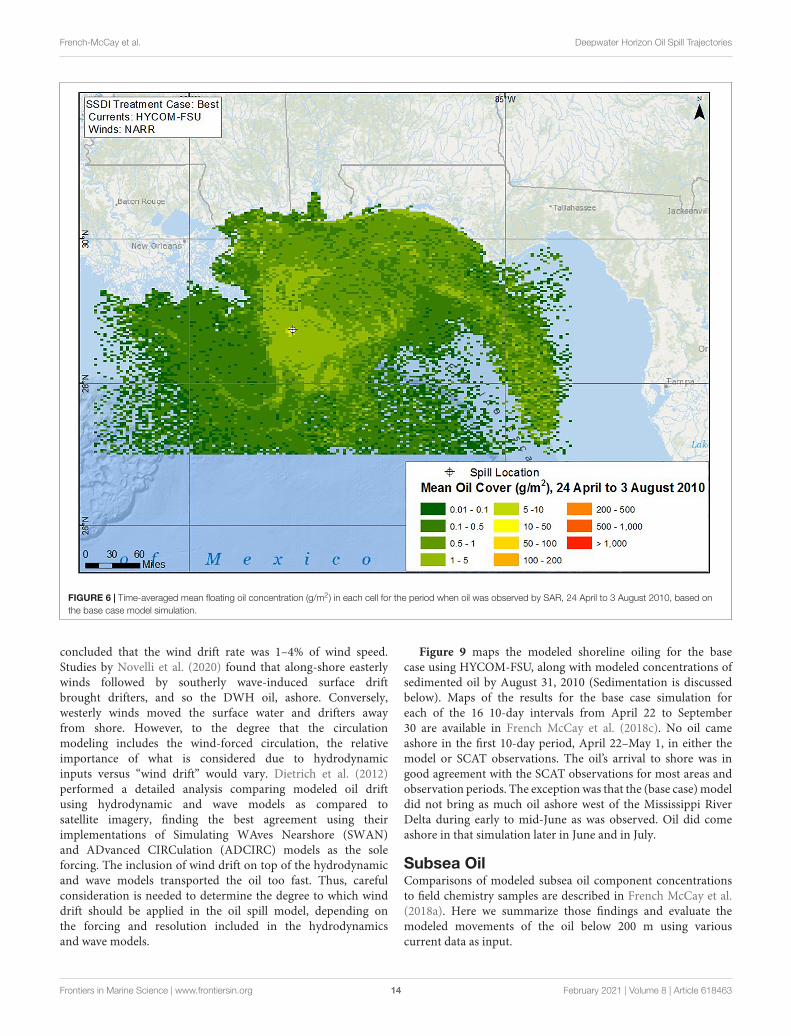
(see the video of the floating oil movements color-coded byage in Supplementary Material) were likely undetected in theremote sensing analyses because of the resolution of thosesensors. The modeled time-averaged mean oil cover (Figure 6)is similar in pattern and of the same magnitudes as theestimates made by MacDonald et al. (2015) based on SARanalysis. Their estimated daily average footprint was 11,200 km2

(SD = 8,430 km2). The model estimate (base case) of the dailyaverage surface area affected by floating oil >1.0 g/m2 was6,720 km2 (SD = 4,960 km2), not significantly different from theremote sensing daily estimate.

Note that the gridded summaries of floating oil distributions,both for the model and for the remote sensing data, providedaverage amounts of oil mass over the cell area. They should notbe interpreted as an actual oil thickness, as the oil is patchyand of varying thicknesses within the cells. The remote sensingdata are typically expressed as volumes per cell for this reason.Furthermore, the total area of the cells where oil is present islarger than the actual oil coverage at any given time. The modeledareas covered by oil, the sum of the areas covered by spillets(representing patches) at a single time step, were an order ofmagnitude lower than those estimated from the gridding. Themean swept area from April 24 to August 3, 2010 (101 days) was1,960 km2/day for the model base case.

The modeled amount of floating oil for the base casesimulation is compared to remote-sensing based estimates inFigure 7. The modeled floating oil volumes, and to somedegree the remote-sensing-based estimates, are inversely relatedto wind speed, as wind events entrain oil into the water and oilaccumulates on the water surface during calm periods. Whilethere is considerable variability in the remote-sensing basedestimates, in large part due to uncertainty in the oil thicknessestimates (Graettinger et al., 2015) used, the model predictionsover time are within the range of the remote-sensing estimates.From May 1 to July 31, 2010, the modeled floating oil volumesaveraged 27,100 m3 (26,500 MT), whereas the remote-sensingbased estimates averaged 25,900 m3. The average floating oilvolumes were 27,700 m3 (27,200 MT) and 29,400 m3 (28,800 MT)for the high and low effectiveness cases, respectively. Withno subsea dispersant use, the model predicted an average of29,800 m3 (29,200 MT) of floating oil in May–July 2010.

Shoreline Oil DistributionsApproximately 2,100 km of beaches and coastal wetlands wereexposed to MC252 oil in 2010, according to the DeepwaterHorizon Natural Resource Damage Assessment Trustee Council(2016; Nixon et al., 2016). The oil was documented by shorelineassessment teams as stranding on 1,773 km of shoreline.Deepwater Horizon Natural Resource Damage AssessmentTrustee Council (2016) mapped maximum observed oiling,categorized as not surveyed, no oil seen, or various degrees ofoiling. Many areas were not surveyed, including much of MobileBay and considerable areas of wetlands in Louisiana. Thus, the2,100 km estimate likely underestimates the actual length ofshoreline affected by oil.

Modeled shoreline oiling results are summarized in Table 2.For simulations run without currents, the length of shoreline







FIGURE 4 | RMSE of relative area and volume (as fractions, panel A) and of oil volume (m3, panel B) for the base case model simulation (using HYCOM-FSU)compared to remote sensing-based data.

oiled is smaller and focused on the area between the MississippiRiver Delta and Alabama. The total length of shore oiledestimated by the Deepwater Horizon Natural Resource DamageAssessment Trustee Council (2016; Nixon et al., 2016) was2,113 km. The categories of degree of oiling used by the Trusteescannot be translated to oil loading amounts (g/m2). The totallengths of shoreline oiling predicted by the model using most ofthe hydrodynamic model currents (except NGOM) are 2,000–2,700 km oiled, with the base case predicting 2,568 km oiled.These results are in good agreement with the observations,considering some areas were not surveyed.

Figure 8 and Supplementary Figures 11–16 summarize thecomparisons of the modeled shoreline oiling with SCAT-basedobservations, showing the variability resulting from differentcurrent and wind inputs. These maps color code where oil cameashore in the model but where the shoreline had not beensurveyed (“no observed coverage, modeled oil”), as well as where

both modeled and observed indicate oil (“match”), where bothobserved and the model indicate no oil (“no observed oil”), wherethere are false negatives (observed only), and where there are falsepositives (modeled only).

The modeled shoreline oiling for the base case compares wellwith the observations (Figure 8), the model showing oiling fromthe Apalachicola Bay area of Florida to Terrebonne Bay areaof Louisiana. Note that the model predicted shore oiling insideMobile Bay in areas where it was not observed. However, as mostof Mobile Bay’s shoreline areas were not surveyed, oiling of thoseareas is unknown. No oil was reported in some of the smallbays along the Florida panhandle. However, booming may haveprevented oil from entering those inlets, whereas booming wasnot included in these model simulations.

Simulations using HYCOM-NRL Reanalysis currents withCFSR winds (Supplementary Figure 11), HYCOM-NRL Real-time currents with NARR winds (Supplementary Figure 12),







FIGURE 5 | Modeled maximum amount of oil in each grid cell at any time in the simulation (as g/m2 averaged over the grid cell), based on the base case modelsimulation.

and NCOM Real-time with NARR winds (SupplementaryFigure 14), predict similar oiling patterns to the base caseusing HYCOM-FSU currents and NARR winds (Figure 8).SABGOM spreads oil to shorelines too far to the east and intowestern Louisiana where no oiling was observed (SupplementaryFigure 13). NGOM currents with NARR winds and the IASROMS simulations carry too much oil to western Louisianaand Texas but otherwise show good agreement with the SCATobservations (Supplementary Figures 15, 16). Simulations madewith no currents, forced with winds only, and those forcedwith ADCP currents and NARR winds, do not bring as muchoil ashore west of the Mississippi River Delta as was observed.Thus, coastal currents prevailing toward the west apparentlytransported the oil to those areas. Also, currents brought theoil east to Florida, as winds alone do not account for thatshoreline oiling.

The shoreline oil distributions were more accurate whenwestward flows near the Mississippi Delta were simulatedin the forcing hydrodynamic model. Novelli et al. (2020)identified westward flows as due to easterly winds. Kourafalouand Androulidakis (2013); Androulidakis and Kourafalou

(2013), and Androulidakis et al. (2015, 2018) examinedand stressed the importance of the Mississippi outflow incontrolling nearshore oil movements and shoreline oilingdistributions. The HYCOM models seemed to have capturedthese dynamics reasonably well in simulating conditions inthe summer of 2010, whereas the ROMS implementationsexamined did not reflect those dynamics. It is possible thatMobile Bay was protected by freshwater outflows not capturedin any of the hydrodynamic models. However, oiling datain Mobile Bay were insufficient to determine how muchentered the bay.

Weisberg et al. (2017) concluded that the general circulationfrom the hydrodynamics modeling could account fortransporting the Deepwater Horizon oil to near shore, butthat the waves, via Stokes drift, were responsible for theactual beaching of the oil. In our analysis, we found the winddrift (i.e., including Ekman flow and Stokes drift) was theprimary driver for bringing oil to shore. Le Heìnaff et al.(2012) and Boufadel et al. (2014) also concluded that winddrift was the most important factor bringing oil ashore. Usingseveral hydrodynamic models as input, Boufadel et al. (2014)







FIGURE 6 | Time-averaged mean floating oil concentration (g/m2) in each cell for the period when oil was observed by SAR, 24 April to 3 August 2010, based onthe base case model simulation.

concluded that the wind drift rate was 1–4% of wind speed.Studies by Novelli et al. (2020) found that along-shore easterlywinds followed by southerly wave-induced surface driftbrought drifters, and so the DWH oil, ashore. Conversely,westerly winds moved the surface water and drifters awayfrom shore. However, to the degree that the circulationmodeling includes the wind-forced circulation, the relativeimportance of what is considered due to hydrodynamicinputs versus “wind drift” would vary. Dietrich et al. (2012)performed a detailed analysis comparing modeled oil driftusing hydrodynamic and wave models as compared tosatellite imagery, finding the best agreement using theirimplementations of Simulating WAves Nearshore (SWAN)and ADvanced CIRCulation (ADCIRC) models as the soleforcing. The inclusion of wind drift on top of the hydrodynamicand wave models transported the oil too fast. Thus, carefulconsideration is needed to determine the degree to which winddrift should be applied in the oil spill model, depending onthe forcing and resolution included in the hydrodynamicsand wave models.

Figure 9 maps the modeled shoreline oiling for the basecase using HYCOM-FSU, along with modeled concentrations ofsedimented oil by August 31, 2010 (Sedimentation is discussedbelow). Maps of the results for the base case simulation foreach of the 16 10-day intervals from April 22 to September30 are available in French McCay et al. (2018c). No oil cameashore in the first 10-day period, April 22–May 1, in either themodel or SCAT observations. The oil’s arrival to shore was ingood agreement with the SCAT observations for most areas andobservation periods. The exception was that the (base case) modeldid not bring as much oil ashore west of the Mississippi RiverDelta during early to mid-June as was observed. Oil did comeashore in that simulation later in June and in July.

Subsea OilComparisons of modeled subsea oil component concentrationsto field chemistry samples are described in French McCay et al.(2018a). Here we summarize those findings and evaluate themodeled movements of the oil below 200 m using variouscurrent data as input.







FIGURE 7 | Volume of surface floating oil, including the oil only or with the water in emulsions, for the base case model and calculated from remote sensing data;wind speeds at NOAA buoy 42040.

Camilli et al. (2010) detected the deep plume at ∼1,000–1,200 m during June 23–27, 2010. Their Sentry’s methane m/zsignal at 35 km from the source was only 53% less than thatat 5.8 km, suggesting that plume extended considerably beyondthe 35 km survey bound at that time. The model using ADCPdata simulated the plume as extending to the southwest 60 kmon June 23 and 82 km on June 27 (video of spillet movementsbelow 900 m in Supplementary Material), consistent with theobservations by Camilli et al. (2010).

While the oil-affected volume has been described as aninverted cone over the well with large droplets rising in thecenter and progressively smaller ones further from the well(e.g., Ryerson et al., 2012; Spier et al., 2013), due to ADCP-documented current shear and varying rise rates for different

TABLE 2 | Shoreline oiling results for model cases, varying currents andwinds used as input.

Currents Winds Length of shoreoiled (km)

Mass of oilashore (MT)

HYCOM-FSU NARR 2,568 64,407

HYCOM-NRL Reanalysis CFSR 1,993 25,045

HYCOM-NRL Real-time NARR 2,698 58,164

SABGOM NARR 2,658 91,677

NCOM Real-time NARR 2,385 85,485

NGOM-NOAA Real-time NARR 3,540 91,089

IAS ROMS NAM 2,507 67,850

ADCPs NARR 1,857 56,189

None NAM 1,436 38,306

None NARR 1,550 49,039

None NOGAPS 1,013 33,483

diameter droplets, “plumes” of rising oil droplets followeddifferent trajectories during their ascent toward the surface, abehavior captured in our model simulations (French McCayet al., 2018a,c). In addition, while rising, the intermediate-sized droplets lost some of their relative buoyancy dueto weathering (dissolution and biodegradation), as well aspotentially combining with SPM in the water column. Theambient current higher in the water column is increasinglystronger than in deep water (Hyun and He, 2010), suchthat the intermediate sized droplets would have separated toform “multiple plumes” of slowly rising droplets in the upperlayers mimicking the deep water plume. Fluorescence anomalies(peaks) and water column hydrocarbon chemistry data (Camilliet al., 2010; Valentine et al., 2010; Spier et al., 2013; as well asNRDA data, Horn et al., 2015 and Payne and Driskell, 2015a,c,2018) showed relatively high concentrations in finite “clouds”of particulate- and dissolved-phase oil at various depths abovethe intrusion at ∼1,100–1,200 m. The SIMAP model simulatedthese behaviors and distribution. Sensitivity analyses by Northet al. (2011, 2015) and Paris et al. (2012) showed similar behavior:droplets with diameters of <50 µm formed distinct subsurfaceplumes that were transported horizontally and remained in thesubsurface for >1 month; while droplets with diameters≥90 µmrose to the surface, more rapidly at larger diameters.

Fluorescence peaks (relative high values) and dissolved oxygen“sags” (relatively low values) in vertical profiles associatedwith elevated hydrocarbon concentrations in water sampleswere consistently observed at depths ∼1,000–1,300 m mainlysouthwest of the wellhead (Joint Analysis Group, 2010; FrenchMcCay et al., 2015a, 2018a; Horn et al., 2015). In the deep plume,the ADCP-measured speeds averaged 3.9 cm/s to the southwest.Measured current speeds were consistently <10 cm/s at all depths







FIGURE 8 | Comparison of model predictions, for the base case simulation using HYCOM-FSU Reanalysis currents and NARR winds, to SCAT-based observationsof cumulative amount of oil coming ashore by September 30, 2010.

and for most of the period of the oil release. ADCP data in ∼30–60 m vertical bins throughout the upper ∼1,000 m of the watercolumn showed currents in adjacent depths differing by as muchas 120◦ in direction during May–June 2010 (French McCay et al.,2015a, 2018a).

In contrast, in the area of the DWH wellhead, allof the hydrodynamic models examined (three HYCOMs:HYCOM_FSU, HYCOM-NRL Reanalysis, HYCOM-NRL Real-time; two ROMS: SABGOM, IAS ROMS; and two POMs:NCOM Real-time, NGOM) calculated much higher speeds forthe currents in the deep plume and water column below 200 mthan is indicated by the ADCPs. Furthermore, the movementswere less consistently toward the southwest than indicated by theADCP and field observation data. This was evident in trajectoriesof oil droplets below 200 m. The video of the oil droplet trajectorybelow 900 m using ADCP data in the Supplementary Materialsummarizes the movements of oil in the deep plume. Snapshotsin the deep plume and at intermediate depths from trajectoriesusing the hydrodynamic models are available in French McCayet al. (2018a,c).

The hydrodynamic models produced current fields below200 m that at times agreed with the ADCP data, and in othertimes diverged in direction and speed. The HYCOM-FSU modelproduced a trajectory of small droplets in deep water (FrenchMcCay et al., 2018a,c) that was most similar to that using theADCP data (video of the oil droplet trajectory below 900 m usingADCP data in Supplementary Material). The ROMs modelstended to transport the small droplets along the bathymetrytoward the southwest in narrow smooth flows much fasterthan indicated by the ADCP data. The IAS ROMS simulation(described in French McCay et al., 2015a, 2016) was very similarto the SABGOM simulation (in French McCay et al., 2018a,c).The HYCOM-NRL Real-time and HYCOM-NRL Reanalysis bothpredicted the deep plume moved primarily northeastward fromApril through July of 2010, such that the modeled deep plumedid not extend southwestward in July as observed (FrenchMcCay et al., 2018c). The POM models (NGOM is shown inFrench McCay et al., 2018a) predicted movements at timesto the northeast and other times to the southwest, but thetiming of movements in these directions did not agree with







FIGURE 9 | Cumulative amount of oil coming ashore and settling to sediments (in g/m2) by August 31, 2010 for the base case simulation using HYCOM-FSUcurrents and NARR winds.

the ADCP and observational data. The NRL NCOM model wassuperseded by NRL’s HYCOM, which produced more realistic(slower) currents at depth, and so the NCOM simulations werenot considered further.

Given the more narrow and accurate surfacing locations (seesection “Floating Oil”), the simulation using ADCPs was the mostrealistic for depths below 200 m. While the interpolation of theADCP data was not a hydrodynamic model, which conservedmass and momentum, the ADCP current data does indicate theactual flow field and which of the hydrodynamic models mostclosely simulated it (i.e., the HYCOM-FSU model).

In the SIMAP model simulations using the ADCP dataand using HYCOM-FSU, the concentrations of droplets anddissolved constituents were highest close to the source (i.e.,∼1,200 or ∼1,300 m). Because the smaller oil droplets werespread out by spatially and time-varying currents as they rosethrough the water column, the modeled concentrations decreasedconsiderably higher in the water column. Oil concentrations inthe deep water were low and in a narrow cylinder stretching

toward the surface in April, when the release was not treatedwith dispersants at the release point and the oil was mostly inthe form of large droplets >0.7 mm in diameter. During Maywhen the kink holes appeared and subsea dispersant began tobe applied, such that small droplets were formed in addition todroplets >0.7 mm in diameter (Spaulding et al., 2015, 2017), themodeled subsurface concentrations were much higher, and thecontamination was dispersed over a wider area. As shown by thesample data (Horn et al., 2015; Payne and Driskell, 2018), thedeep plume of small droplets and dissolved components persistedfrom May to July. The model results show more extensive plumesin deep water in June–July when more effective subsea dispersantapplications were used than prior to June 3. See French McCayet al. (2015a, 2016, 2018a,c) for further detail and maps depictingthe concentration distributions in space and time.

Oil SedimentationOil from the DWH spill was identified in the sediments inthe offshore area surrounding and down-stream of the well site







(Joye et al., 2011; Montagna et al., 2013; Valentine et al., 2014;Romero et al., 2015; Stout and Payne, 2016a; Stout et al., 2016b).Valentine et al. (2014) noted that the pattern of contaminationindicates deep-ocean intrusion layers as the source, consistentwith deposition of a “bathtub ring” formed from an oil-rich layerof water impinging laterally upon the continental slope (at adepth of∼900–1,300 m) and a higher-flux “fallout plume” whereoil-SPM aggregates sank to underlying sediment (at a depth of∼1,300–1,700 m).

Figure 9 maps the modeled sedimentation by August 31,2010 for the base case using HYCOM-FSU for surface watersand ADCP data in deep water. The modeled sedimentationin deep water due to fallout by interactions with SPMand the bathtub ring impingement was in consistentlocations to those mapped by Valentine et al. (2014),Stout et al. (2016a), and Romero et al. (2015). The modelalso predicted considerable sedimentation in the nearshorewaters of Louisiana.

CONCLUSION

Summary of FindingsThe modeled spatial distribution of surface oil was validatedby comparison to remote sensing data. As the model rancontinuously from April 22 through September of 2010,disagreement would be expected for older oil. However, freshlysurfacing oil reset the modeled origin of the slicks on acontinuous basis. The results indicate the importance of thewind drift in transporting the floating oil northward towardshore (consistent with Dietrich et al., 2012; Le Heìnaff et al.,2012; Boufadel et al., 2014; Weisberg et al., 2017), but thatthe currents used can change the patterns considerably. Themodel-predicted amount of floating oil agreed with remote-sensing based estimates, confirming the modeled DSDs and fateprocesses were realistic.

The modeled shoreline oiling for the base case (∼2,600 kmoiled) compares well with the observations (∼2,100 km oiled;Nixon et al., 2016), with the model showing oiling from theApalachicola Bay to Terrebonne Bay. The model predicted oilingon shore in areas that were not surveyed, so oiling of those areasbased on observations is unknown. Other model simulationsdemonstrated the variability resulting from different current andwind inputs. Shoreline oiling events were discontinuous andoccurred when winds (via wind drift) carried oil onshore.

Simulations of subsurface oil movements using current datafrom seven hydrodynamic models resulted in very differenttrajectories, and to varying degrees the hydrodynamic modelsgenerally over-estimated the speed of the currents in the areaof the wellhead. Published DWH oil trajectory simulations(MacFadyen et al., 2011; Mariano et al., 2011; North et al.,2011, 2015; Dietrich et al., 2012; Le Heìnaff et al., 2012;Paris et al., 2012; Boufadel et al., 2014; Lindo-Atichati et al.,2014; Testa et al., 2016; Weisberg et al., 2017) show highlyvariable paths and concentrations as well. MacFadyen et al.(2011); Mariano et al. (2011), Le Heìnaff et al. (2012); Dietrichet al. (2012), Boufadel et al. (2014), and Weisberg et al. (2017)

compared their predicted surface oil movements to field data,finding wind drift to be important to transport, along withthe hydrodynamic model produced currents. However, they didnot analyze subsea movements of the oil in comparison toobservations. In our modeling studies, the base case simulationusing currents generated by the HYCOM-FSU hydrodynamicsmodel (Chassignet and Srinivasan, 2015) consistently resulted inboth a subsea trajectory and concentration fields most similarto that predicted by the ADCP measurement-based current fieldbelow 200 m. The flow was generally toward the southwest, asthe ADCPs indicated occurred (French McCay et al., 2018a).The HYCOM used by Paris et al. (2012), which was apparentlythe same HYCOM-NRL Real-time product we used, also showedsimilar movements of small droplets in the deep plume.

Because most of oil forming the surface slicks was from largedroplets that surfaced near well, it was not very displaced bydeep currents. Thus, use of the various hydrodynamic modelsfor transport below 200 m did not greatly influence the surfacinglocations to the point where it would be perceptible in the overalldistribution of floating oil (i.e., as compared to synoptic remote-sensing based maps of oil distributions). Thus, the modelingproblem can be treated in two domains: waters below 200 m inthe offshore and surface waters above 200 m both offshore andover the shelf to nearshore.

Implications for Modeling EnvironmentalExposuresThis modeling effort is unique and ground-breaking in severalways. The objective is to quantify by modeling oil transport,fate, exposure concentrations, and (as part of follow-on studies)biological effects (French McCay et al., 2015a,b,c,d,e being thefirst syntheses of these efforts). Thus, the modeling predicted oiltransport, fate and exposures continuously over the entire spillperiod, including in deep water and surface waters. Transportmodeling evaluated nine potential hydrodynamic inputs (sevenmodels, measurement data and an assumption of no currents).The complexities of the oil composition and weatheringwere tracked using pseudo-components, such that exposureconcentrations could be characterized by concentrations of eachpseudo-component in the mixtures. Most fate processes werequantified as well, as opposed to evaluating implications ofcertain assumed inputs, such as droplet size or biodegradationrates. However, some fate processes could not be quantifiedfor lack of sufficient information, such as related to marineoil snow formation and its flux to the sea floor. The exposuremodeling (French McCay et al., 2015b,c) involved distribution,behavioral analysis and simulation of movements of manybiological groups and life stages, recording their exposurehistories to oil components, the results of which are beinganalyzed. We have also made a concerted effort to validate themodel simulations at each stage of the overall effort. Such acomprehensive modeling and validation exercise has not beenattempted previously.

The importance of data assimilation is well-established forcalibrating physical models with observational information, andthe tested and literature-reported hydrodynamic models do







include assimilation of such information as sea surface heightand temperature. However, data assimilation techniques havenot been applied in oil spill models. Rather, many of theliterature-reported oil trajectory model exercises (such as someof those noted above) ran short-term trajectories from knownoil positions, as opposed to long simulations where displacementerrors would compound. MacFadyen et al. (2011) describedtheir approach for modeling during the response period wheretrajectories were reinitialized from identified remote sensing-based observations, and different hydrodynamic models wereused over time, in order to obtain the more accurate trajectories.

While such a nudging-based initialization approach wasconsidered and tested, whereby oil positions were updated withremote sensing observations, as was done for the responsemodeling (MacFadyen et al., 2011), this led to discontinuities inthe concentrations of oil on the surface and in the water columnbeneath it. Thus, the exposures to biota were not reflective ofreality and under-estimated when oil was repositioned. Further,weathering history of each oil spillet was needed to evaluatethe composition of the exposure concentrations. Remote sensinganalyses did identify thick and thin oil but did not provideenough information to track which parcel of oil moved where,such that weathered versus fresh oil could be tracked andrepositioned appropriately. Thus, a more sophisticated “nudging”approach would be needed to improve the oil trajectory over whatwould be predicted from the hydrodynamic modeled currentsand meteorological models wind products.

However, the predicted surface oil distributions werereasonable as compared to the remote sensing and shorelineoiling data. This suggests that the data assimilation techniquesemployed by the hydrodynamic and meteorological modelswere sufficient to produce reliable oil trajectories. On-goingimprovements in hydrodynamic modeling and data assimilationtechniques should continue to improve oil spill model predictionsof oil movements in the surface layer.

On the whole, the predictions of subsurface oil movementbelow 200 m were not nearly as reliable as for the floatingoil. A major limitation is the availability of measurementdata to assimilate into the hydrodynamic models. ADCP,temperature and salinity measurements throughout the watercolumn in deep water over the full domain of interest couldallow data assimilation to tune the hydrodynamics to betterreflect the field conditions. Data assimilative techniques havebeen included in all seven of the hydrodynamic modelsevaluated, but likely these will need more developmentto handle the deep-water three-dimensional flow fields. Inaddition, analysis techniques are needed for evaluating modelperformance in simulating deep-water flows, analogous tothose used for surface water dynamics (e.g., Halliwell et al.,2014).

With respect to quantifying exposures and biological effects,the results will depend on the areas and volumes affected atexposure concentrations that potentially could cause adverseeffects (French McCay et al., 2004; French McCay, 2009). Ifbiota have similar densities in areas affected by the model,as in areas oiled in the field, then the modeling results willbe reliable, even if the specific path of the floating oil or

subsurface plume is not precisely located. For wildlife, themodeled swept area by surface oil determines numbers ofanimals affected. For water column biota, the effects arerelated to the volume exceeding concentrations of concern.Biological densities are more uniform (on average) in offshorepelagic waters than they would be near the coast. Thus,accuracy of the trajectory and exposure concentrations aremore important nearshore than in open waters offshore. Themodeled movements and amounts of oil floating over timewere found to be in good agreement with estimates frominterpretation of remote sensing data, indicating initial oildroplet distributions and oil transport and fate processesproduced oil distribution results reliable for evaluatingenvironmental exposures in the water column and fromfloating oil at water surface.

Both organisms and oil components are highly patchy andvariable over time. Present models cannot deterministicallypredict these fine scale dynamics. Further, biological distributiondata are not available to precisely quantify fine scale distributionsof all species and life stages. However, statistically describing theoil exposures, toxicological effects, and biological distributionsshould lead to reliable results. This approach also allowsquantification of the uncertainties related to potential adverseeffects. Model analyses have demonstrated the importance ofthe currents, winds and initial DSD to exposure concentrations,and have provided best estimates and uncertainty bounds forassessments. Analyses of potential exposures and biologicaleffects based on these validated oil fate simulations usingHYCOM-FSU and ADCP data are being developed, usingmethods and data similar to those described in French McCayet al. (2015b,c,d), such that the impacts of the DWH oil spill canbe better understood.

DATA AVAILABILITY STATEMENT

Publicly available datasets were analyzed in this study. Thisdata can be found here: The remote sensing, ShorelineCleanup and Assessment, sensor and chemistry datasetsanalyzed for this study can be found in the ERMA Repository:The ERMA R© Deepwater Gulf Response Web Application.https://erma.noaa.gov/gulfofmexico/erma.html#/layers=3+10717+16023+17774+32237+32238+32239+32240&x=−89.48747&y=27.92566&z=6.4&panel=layer and https://erma.noaa.gov/admin/folder/4481. Folder Name DWH Remote Sensing ProductsFolder Path Deepwater Horizon MC 252 Incident > Imagery &Remote Sensing Products > DWH Remote Sensing Products.

AUTHOR CONTRIBUTIONS

DF, MS, and DM designed the study. DF, MS, DC, DM, MH, andJF analyzed the data. DF wrote the manuscript. All authors listedhave made a substantial, direct and intellectual contribution tothe work, and approved it for publication.


https://erma.noaa.gov/gulfofmexico/erma.html#/layers=3+10717+16023+17774+32237+32238+32239+32240&x=-89.48747&y=27.92566&z=6.4&panel=layer



https://erma.noaa.gov/admin/folder/4481

https://erma.noaa.gov/admin/folder/4481






FUNDING

Funding of this research was provided in part by the NationalOceanic and Atmospheric Administration Damage Assessment,Remediation and Restoration Program (NOAA Contract No.AB133C-11-CQ-0050), and in part by the United StatesDepartment of the Interior, Bureau of Ocean EnergyManagement, Environmental Studies Program, Washington,DC (BOEM Contract Number M11PC00028). Some of theinformation developed was used in the development of the DraftProgrammatic Damage Assessment and Restoration Plan/DraftProgrammatic Environmental Impact Statement (pDARP,Deepwater Horizon Natural Resource Damage AssessmentTrustee Council, 2016) for the DWH spill. The opinionsexpressed by the authors are their own and do not necessarilyreflect the opinion or policy of the U.S. Government. Any use oftrade, firm, or product names is for descriptive purposes only anddoes not imply endorsement by the U.S. Government.

ACKNOWLEDGMENTS

The authors acknowledge the contributions of Katherine Jayko,Cheryl Morse, and Tatsu Isaji of RPS for model code preparation,testing and debugging. Zhengkai Li and Yong Kim, formerlyof RPS, contributed to data collection, quality control, andcompilation efforts used to provide model inputs. RachelShmookler, also formerly of RPS, performed computationsrelated to the shoreline oiling data. We thank three reviewersfor their constructive comments, which improved the clarity ofthis manuscript.

SUPPLEMENTARY MATERIAL

The Supplementary Material for this article can be foundonline at: https://www.frontiersin.org/articles/10.3389/fmars.2021.618463/full#supplementary-material

REFERENCESAdams, E. E., Socolofsky, S. A., and Boufadel, M. (2013). Comment on “Evolution

of the macondo well blowout: simulating the effects of the circulation andsynthetic dispersants on the subsea oil transport”. Environ. Sci. Technol. 47,11905–11905. doi: 10.1021/es4034099

Adcroft, A., Hallberg, R., Dunne, J. P., Samuels, B. L., Galt, J. A., Barker, C. H., et al.(2010). Simulations of underwater plumes of dissolved oil in the Gulf of Mexico.Geophys. Res. Lett. 37:L18605. doi: 10.1029/2010GL044689

Allen, A. A., Mabile, N. J., Jaeger, D., and Costnzo, D. (2011). The use of controlledburning during the Gulf of Mexico Deepwater Horizon MC-252 oil spillresponse. Int. Oil Spill Conf. Proc. 2011:abA194. doi: 10.7901/2169-3358-2011-1-194

Aman, Z. M., Paris, C. B., May, E. F., Johns, M. L., and Lindo-Atichati, D. (2015).High-pressure visual experimental studies of oil-in-water dispersion dropletsize. Chem. Eng. Sci. 127, 392–400.

Androulidakis, Y., Kourafalou, V., Ozgokmen, T., Garcia-Pineda, O., Lund, B.,Le Hénaff, M., et al. (2018). Influence of river-induced fronts on hydrocarbontransport: a multiplatform observational study. J. Geophys. Res. Oceans 123,3259–3285. doi: 10.1029/2017JC013514

Androulidakis, Y. S., and Kourafalou, V. H. (2013). On the processes that influencethe transport and fate of Mississippi waters under flooding outflow conditions.Ocean Dyn. 63, 143–164. doi: 10.1007/s10236-012-0587-8

Androulidakis, Y. S., Kourafalou, V. H., and Schiller, R. V. (2015). Process studieson the evolution of the Mississippi River plume: impact of topography, windand discharge conditions. Cont. Shelf Res. 107, 33–49. doi: 10.1016/j.csr.2015.07.014

Belore, R. C., Trudel, B. K., and Morrison, J. (2011). Weathering, emulsification,and chemical dispersibility of Mississippi Canyon 252 crude oil: field andLaboratory studies. Int. Oil Spill Conf. Proc. 2011:abs247. doi: 10.7901/2169-3358-2011-1-247

Boufadel, M. C., Abdollahi-Nasab, A., Geng, X., Galt, J., and Torlapati, J. (2014).Simulation of the landfall of the deepwater horizon oil on the shorelines of theGulf of Mexico. Environ. Sci. Technol. 48, 9496–9505. doi: 10.1021/es5012862

Boyer, T., Levitus, S., Garcia, H., Locarnini, R. A., Stephens, C., and Antonov, J.(2004). Objective analyses of annual, seasonal, and monthly temperature andsalinity for the World Ocean on a 1

4 E Grid. Int. J. Climatol. 25, 931–945.Camilli, R., Reddy, C. M., Yoerger, D. R., Van Mooy, B. A. S., Jakuba, M. V., Kinsey,

J. C., et al. (2010). Tracking hydrocarbon plume transport and biodegradationat Deepwater Horizon. Science 330, 201–204. doi: 10.1126/science.1195223

Chao, Y., He, R., Farrara, J., and Zhang, C. (2014). ROMS Hydrodynamic Modeling.Report to NOAA OR&R NRDA Program. Saint Petersburg, FL: National Oceanicand Atmospheric Administration, 64.

Chao, Y., Li, Z., Farrara, J. D., McWilliams, J. C., Bellingham, J., Capet,X., et al. (2009). Development, implementation and evaluation of a

data-assimilative ocean forecasting system off the central Californiacoast. Deep Sea Res. II 56, 100–126. doi: 10.1016/j.dsr2.2008.08.011

Chassignet, E. P., Hurlburt, H. E., Metzger, E. J., Smedstad, O. M., Cummings,J. A., Halliwell, G. R., et al. (2009). US GODAE: global ocean prediction withthe HYbrid Coordinate Ocean Model (HYCOM). Oceanography 22, 64–75.doi: 10.5670/oceanog.2009.39

Chassignet, E. P., and Srinivasan, A. (2015). Data Assimilative Hindcast for the Gulfof Mexico. US Dept. of the Interior, Bureau of Ocean Energy Management, OCSStudy BOEM 2015-035. Sterling VA: BOEM, 40.

Csanady, G. T. (1973). Turbulent Diffusion in the Environment. Dordrecht: D.Reidel Publishing Company.

Daae, R. L., Skancke, J., Brandvik, P. J., and Faksness, L.-G. (2018). The sensitivityof the surface oil signature to subsurface dispersant injection and weatherconditions. Mar. Pollut. Bull. 127, 175–181. doi: 10.1016/j.marpolbul.2017.11.067

Deepwater Horizon Natural Resource Damage Assessment TrusteeCouncil, (2016). The Deepwater Horizon Oil Spill Final ProgrammaticDamage Assessment and Restoration Plan and Final ProgrammaticEnvironmental Impact Statement. National Oceanic and AtmosphericAdministration, Office of Response and Restoration. Available online at:http://www.gulfspillrestoration.noaa.gov/restoration-planning/gulf-plan/(accessed July 10, 2016).

Diercks, A. R., Highsmith, R. C., Asper, V. L., Joung, D., Zhou, Z., Guo, L.,et al. (2010). Characterization of subsurface polycyclic aromatic hydrocarbonsat the Deepwater Horizon site. Geophys. Res. Lett. 37:L20602. doi: 10.1029/2010GL045046

Dietrich, J. C., Trahana, C. J., Howard, M. T., Fleming, J. G., Weaver, R. J., Tanakae,D. S., et al. (2012). Surface trajectories of oil transport along the northerncoastline of the Gulf of Mexico. Cont. Shelf Res. 41, 17–47. doi: 10.1016/j.csr.2012.03.015

Driskell, W. B., and Payne, J. R. (2018). Macondo oil in northern Gulf of Mexicowaters – part 2: dispersant-accelerated PAH dissolution in the DeepwaterHorizon plume. Mar. Pollut. Bull. 129, 412–419. doi: 10.1016/j.marpolbul.2018.02.057

ERMA, (2016). The ERMA§Deepwater Gulf Response Web Application. Tokyo:ERMA.

Fingas, M., and Fieldhouse, B. (2012). Studies on water-in-oil products from crudeoils and petroleum products. Mar. Pollut. Bull. 64, 272–283. doi: 10.1016/j.marpolbul.2011.11.019

Fitzpatrick, J. J. (2009). Assessing skill of estuarine and coastal eutrophicationmodels for water quality managers. J. Mar. Syst. 76, 195–211. doi: 10.1016/j.jmarsys.2008.05.018

French, D., Reed, M., Jayko, K., Feng, S., Rines, H., Pavignano, S., et al. (1996).The CERCLA type A Natural Resource Damage Assessment Model for Coastal


https://www.frontiersin.org/articles/10.3389/fmars.2021.618463/full#supplementary-material

https://www.frontiersin.org/articles/10.3389/fmars.2021.618463/full#supplementary-material

https://doi.org/10.1021/es4034099

https://doi.org/10.1029/2010GL044689

https://doi.org/10.7901/2169-3358-2011-1-194

https://doi.org/10.7901/2169-3358-2011-1-194

https://doi.org/10.1029/2017JC013514

https://doi.org/10.1007/s10236-012-0587-8

https://doi.org/10.1016/j.csr.2015.07.014


https://doi.org/10.7901/2169-3358-2011-1-247

https://doi.org/10.7901/2169-3358-2011-1-247

https://doi.org/10.1021/es5012862

https://doi.org/10.1126/science.1195223

https://doi.org/10.1016/j.dsr2.2008.08.011


https://doi.org/10.5670/oceanog.2009.39

https://doi.org/10.1016/j.marpolbul.2017.11.067


http://www.gulfspillrestoration.noaa.gov/restoration-planning/gulf-plan/

https://doi.org/10.1029/2010GL045046

https://doi.org/10.1029/2010GL045046







https://doi.org/10.1016/j.jmarsys.2008.05.018







and Marine Environments (NRDAM/CME), Technical Documentation, Vol. I -V. Final Report, submitted to the Office of Environmental Policy and Compliance,U.S. Dept. of the Interior, Washington, DC, April, 1996. Springfield, VA: NationalTechnical Information Service,

French McCay, D., Horn, M., Li, Z., Crowley, D., Spaulding, M., Mendelsohn, D.,et al. (2018c). Simulation Modeling of Ocean Circulation and Oil Spills in theGulf of Mexico, Volume III: Data Collection, Analysis and Model Validation. NewOrleans, LA: US Department of the Interior, 313.

French McCay, D., Jayko, K., Li, Z., Horn, M., Isaji, T., and Spaulding, M. (2018b).“Volume II: appendix II – oil transport and fates model technical manual,” inSimulation Modeling of Ocean Circulation and Oil Spills in the Gulf of Mexico,eds C. W. Galagan, D. French McCay, J. Rowe, and L. McStay, (New Orleans,LA: US Department of the Interior), 422.

French McCay, D., Whittier, N., Sankaranarayanan, S., Jennings, J., and Etkin, D. S.(2004). Estimation of potential impacts and natural resource damages of oil.J. Hazardous Mater. 107, 11–25. doi: 10.1016/j.jhazmat.2003.11.013

French McCay, D. P. (2003). Development and application of damage assessmentmodeling: example assessment for the north cape oil spill. Mar. Pollut. Bull. 47,341–359. doi: 10.1016/s0025-326x(03)00208-x

French McCay, D. P. (2004). Oil spill impact modeling: development andvalidation. Environ. Toxicol. Chem. 23, 2441–2456. doi: 10.1897/03-382

French McCay, D. P., Jayko, K., Li, Z., Horn, M., Kim, Y., Isaji, T., et al. (2015a).Technical Reports for Deepwater Horizon Water Column Injury Assessment –WC_TR14: Modeling Oil Fate and Exposure Concentrations in the DeepwaterPlume and Cone of Rising Oil Resulting from the Deepwater Horizon OilSpill. DWH NRDA Water Column Technical Working Group Report. Preparedfor National Oceanic and Atmospheric Administration by RPS ASA, SouthKingstown, RI, USA. September 29, (2015a). Administrative Record no. DWH-AR0285776. Washington, DC: U.S. Department of the Interior.

French McCay, D. P., Li, Z., Horn, M., Crowley, D., Spaulding, M., Mendelsohn, D.,et al. (2016). “Modeling oil fate and subsurface exposure concentrations fromthe Deepwater Horizon oil spill,” in Proceedings of the 39th AMOP TechnicalSeminar on Environmental Contamination and Response, Vol. 39, (Ottawa, ON:Environment Canada), 115–150.

French McCay, D., Crowley, D., and McStay, L. (2019). Sensitivity of modeled oilfate and exposure from a subsea blowout to oil droplet sizes, depth, dispersantuse, and degradation rates. Mar. Pollut. Bull. 146, 779–793. doi: 10.1016/j.marpolbul.2019.07.038

French McCay, D., Crowley, D., Rowe, J., Bock, M., Robinson, H., Wenning, R.,et al. (2018d). Comparative risk assessment of spill response options for adeepwater oil well blowout: Part I. Oil spill modeling. Mar. Pollut. Bull. 133,1001–1015. doi: 10.1016/j.marpolbul.2018.05.042

French McCay, D., Horn, M., Li, Z., Jayko, K., Spaulding, M., Crowley, D., et al.(2018a). “Modeling distribution fate and concentrations of deepwater horizonoil in subsurface waters of the Gulf of Mexico,” in Chapter 31 in Oil SpillEnvironmental Forensics Case Studies, eds S. Stout, and Z. Wang, (Amsterdam:Elsevier), 683–736. doi: 10.1016/b978-0-12-804434-6.00031-8

French McCay, D., Rowe, J., Balouskus, R., Morandi, A., and McManus,R. C. (2015e). Technical Reports for Deepwater Horizon Water ColumnInjury Assessment – WC_TR.28: Injury Quantification for Planktonic Fishand Invertebrates in Estuarine, Shelf and Offshore Waters. DWH NRDAWater Column Technical Working Group Report. Prepared for NationalOceanic and Atmospheric Administration by RPS ASA, South Kingstown, RI,USA. Administrative Record no. DWH-AR0172019.pdf, DWH-AR0172219.xlsx-DWH-AR0172227.xlsx. Washington, DC: U.S. Department of the Interior.

French McCay, D. P. (2009). “State-of-the-art and research needs for oil spillimpact assessment modeling,” in Proceedings of the 32nd AMOP TechnicalSeminar on Environmental Contamination and Response, Emergencies ScienceDivision, (Ottawa, ON: Environment Canada), 601–653.

French McCay, D. P., Balouskus, R., McManus, M. C., Schroeder, M., Rowe,J. J., and Bohaboy, E. (2015d). Technical Reports for Deepwater HorizonWater Column Injury Assessment – WC_TR.12: Evaluation of ProductionForegone as the Result of Direct Kill of Fish and Invertebrate Individuals. DWHNRDA Water Column Technical Working Group Report. Prepared for NationalOceanic and Atmospheric Administration by RPS ASA, South Kingstown, RI,USA. Administrative Record no. DWH-AR0285169.pdf, DWH-AR0285305.xlsx-DWH-AR0285361.xlsx. Washington, DC: U.S. Department of the Interior.

French McCay, D. P., McManus, M. C., Balouskus, R., Rowe, J. J., Schroeder, M.,Morandi, A., et al. (2015c). Technical Reports for Deepwater Horizon WaterColumn Injury Assessment: WC_TR.10: Evaluation of Baseline Densities for

Calculating Direct Injuries of Aquatic Biota During the Deepwater Horizon OilSpill. DWH NRDA Water Column Technical Working Group Report. Preparedfor National Oceanic and Atmospheric Administration by RPS ASA, SouthKingstown, RI, USA. Administrative Record no. DWH-AR0285021.pdf, DWH-AR0285141.xlsx, DWH-AR02851412.xlsx. Washington, DC: U.S. Departmentof the Interior.

French McCay, D. P., Morandi, A., McManus, M. C., Schroeder Gearon, M.,Jayko, K., and Rowe, J. J. (2015b). Technical Reports for Deepwater HorizonWater Column Injury Assessment – WC_TR.09: Vertical Distribution Analysisof Plankton. DWH NRDA Water Column Technical Working Group Report.Prepared for National Oceanic and Atmospheric Administration by RPS ASA,South Kingstown, RI, USA. DWH NRDA Water Column Technical WorkingGroup Report. Prepared for National Oceanic and Atmospheric Administrationby RPS ASA, South Kingstown, RI, USA. Administrative Record no. DWH-AR0195958.pdf, DWH-AR0171921.xlsx, DWH-AR0171922.xlsx. Washington,DC: U.S. Department of the Interior.

Garcia-Pineda, O., MacDonald, I., Hu, C., Svejkovsky, J., Hess, M., Dukhovskoy,D., et al. (2013a). Detection of floating oil anomalies from the DeepwaterHorizon oil spill with synthetic aperture radar. Oceanography 26, 124–137.doi: 10.5670/oceanog.2013.38

Garcia-Pineda, O., MacDonald, I., Zimmer, B., Shedd, B., and Roberts, H. (2010).Remote sensing evaluation of geophysical anomaly sites in the outer continentalslope, northern Gulf of Mexico. Deep Sea Res. II Top. Stud. Oceanogr. 57,1859–1869. doi: 10.1016/j.dsr2.2010.05.005

Garcia-Pineda, O., MacDonald, I. R., Li, X., Jackson, C. R., and Pichel, W. G.(2013b). Oil spill mapping and measurement in the Gulf of Mexico with texturalclassifier neural network algorithm (TCNNA). IEEE J. Select. Top. Appl. EarthObserv. Rem. Sens. 6, 2517–2525. doi: 10.1109/jstars.2013.2244061

Garcia-Pineda, O., Zimmer, B., Howard, M., Pichel, W., Li, X., and MacDonald,I. R. (2009). Using SAR images to delineate ocean oil slicks with a textureclassifying neural network algorithm (TCNNA). Can. J. Rem. Sens. 35, 411–421.doi: 10.5589/m09-035

General Bathymetric Chart of the Oceans, (2009). Centenary Edition of the GEBCODigital Atlas. Published on behalf of the Intergovernmental OceanographicCommission (IOC) and the International Hydrographic Organization (IHO)as part of the General Bathymetric Chart of the Oceans. Liverpool: BritishOceanographic Data Centre.

Goni, G. J., Trinanes, J. A., MacFadyen, A., Streett, D., Olascoaga, M. J., Imhoff,M. L., et al. (2015). “Variability of the deepwater horizon surface oil spill extentand its relationship to varying ocean currents and extreme weather conditions,”in Mathematical Modelling and Numerical Simulation of Oil Pollution Problems,ed. M. Ehrhardt, (Cham: Springer International Publishing Switzerland), 1–22.doi: 10.1007/978-3-319-16459-5_1

Graettinger, G., Holmes, J., Garcia-Pineda, O., Hess, M., Hu, C., Leifer, I., et al.(2015). Integrating Data from Multiple Satellite Sensors to Estimate Daily Oilingin the Northern Gulf of Mexico during the Deepwater Horizon Oil Spill. DWHNatural Resource Exposure NRDA Technical Working Group Report, FE_TR.31.Washington, DC: NOAA, 46.

Gros, J., Socolofsky, S. A., Dissanayake, A. L., Jun, I., Zhao, L., Boufadel, M. C.,et al. (2017). Petroleum dynamics in the sea and influence of subsea dispersantinjection during Deepwater Horizon. Proc. Natl. Acad. Sci. U.S.A. 114, 10065–10070. doi: 10.1073/pnas.1612518114

Halliwell, G. R. Jr., Srinivasan, A., Kourafalou, V., Yang, H., Willey, D., Le Hénaff,M., et al. (2014). Rigorous evaluation of a fraternal twin ocean OSSE systemfor the open Gulf of Mexico. J. Atmos. Oceanic Technol. 31, 105–130. doi:10.1175/JTECH-D-13-00011

Horn, M., French McCay, D., Payne, J., Driskell, W., Li, Z., Grennan, M.,et al. (2015). Technical Reports for Deepwater Horizon Water Column InjuryAssessment –Volume III. Water Column Chemical and Physical Data fromthe Deepwater Horizon Blowout. RPS ASA, South Kingstown, RI, USA,August (2015). DWH-AR0024617.pdf (main), DWH-AR0024364.pdf (AppendixB), DWH-AR0024462.pdf (Appendix C), DWH-AR0023990.pdf (Appendix D).Washington, DC: U.S. Department of the Interior.

Hyun, K. H., and He, R. (2010). Coastal upwelling in the South Atlantic Bight: arevisit of the 2003 cold event using long term observations and model hindcastsolutions. J. Mar. Syst. 83, 1–13. doi: 10.1016/j.jmarsys.2010.05.014

Johansen, O., Brandvik, P., and Farook, U. (2013). Droplet breakup in subsea oilreleases – Part 2: predictions of droplet size distributions with and withoutinjection of chemical dispersants. Mar. Pollut. Bull. 73, 327–335. doi: 10.1016/j.marpolbul.2013.04.012


https://doi.org/10.1016/j.jhazmat.2003.11.013

https://doi.org/10.1016/s0025-326x(03)00208-x

https://doi.org/10.1897/03-382




https://doi.org/10.1016/b978-0-12-804434-6.00031-8



https://doi.org/10.1109/jstars.2013.2244061

https://doi.org/10.5589/m09-035

https://doi.org/10.1007/978-3-319-16459-5_1

https://doi.org/10.1073/pnas.1612518114

https://doi.org/10.1175/JTECH-D-13-00011

https://doi.org/10.1175/JTECH-D-13-00011









Joint Analysis Group, (2010). Joint Analysis Group (JAG) Review of R/V BrooksMcCall Data to Examine Subsurface Oil. Available online at: http://www.ncddc.noaa.gov/activities/healthy-oceans/jag/reports/ (accessed November 1, 2011).

Jolliff, J. K., Smith, T. A., Ladner, S., and Arnone, R. A. (2014). Simulating surfaceoil transport during the Deepwater Horizon oil spill: experiments with theBioCast system. Ocean Modell. 75, 84–99. doi: 10.1016/j.ocemode.2014.01.004

Joye, S. I, MacDonald, R., Leifer, I., and Asper, V. (2011). Magnitude and oxidationpotential of hydrocarbon gases released from the bp oil well blowout. Nat.Geosci. 4, 160–164. doi: 10.1038/ngeo1067

Kourafalou, V. H., and Androulidakis, Y. S. (2013). Influence of Mississippi Riverinduced circulation on the Deepwater Horizon oil spill transport. J. Geophys.Res. 118, 3823–3842. doi: 10.1002/jgrc.20272

Le Heìnaff, M., Kourafalou, V. H., Paris, C. B., Helgers, J., Aman, Z. M., Hogan,P. J., et al. (2012). Surface evolution of the Deepwater Horizon oil spill patch:combined effects of circulation and wind-induced drift. Environ. Sci. Technol.46, 7267–7273. doi: 10.1021/es301570w

Ledwell, J. R., He, R., Xue, Z., DiMarco, S. F., Spencer, L. J., and Chapman, P. (2016).Dispersion of a tracer in the deep Gulf of Mexico. J. Geophys. Res. Oceans 121,1110–1132. doi: 10.1002/2015jc011405

Lehr, W., Bristol, S., and Possolo, A., (2010). Oil Budget Calculator,Deepwater Horizon, Technical Documentation. A Report to the NationalIncident Command. The Federal Interagency Solutions Group, OilBudget Calculator Science and Engineering Team. Available onlineat: http://www.restorethegulf.gov/sites/default/files/documents/pdf/OilBudgetCalc_Full_HQ-Print_111110.pdf (accessed on April 1, 2012)

Li, Z., Spaulding, M., and French McCay, D. (2017b). An algorithm for modelingentrainment and naturally and chemically dispersed oil droplet size distributionunder surface breaking wave conditions. Mar. Pollut. Bull. 119, 145–152. doi:10.1016/j.marpolbul.2017.03.048

Li, Z., Spaulding, M. L., French McCay, D., Crowley, D., and Payne, J. R. (2017a).Development of a unified oil droplet size distribution model with applicationto surface breaking waves and subsea blowout releases considering dispersanteffects. Mar. Pollut. Bull. 114, 247–257. doi: 10.1016/j.marpolbul.2016.09.008

Lindo-Atichati, D., Paris, C. B., Le Hénaff, M., Schedler, M., Valladares Juárez,A. G., and Müller, R. (2014). Simulating the effects of droplet size, high-pressurebiodegradation, and variable flow rate on the subsea evolution of deep plumesfrom the Macondo blowout. Deep Sea Res. II Top. Stud. Oceanogr. 129, 301–310.doi: 10.1016/j.dsr2.2014.01.011

Liu, Y., Weisberg, R. H., Hu, C., and Zheng, L. (2011). Tracking the DeepwaterHorizon Oil spill: a modeling perspective. Eos Trans. Am. Geophys. Union 92,45–46. doi: 10.1029/2011eo060001

Mabile, N., and Allen, A. (2010). Controlled Burns After Action Report, Burns onMay 28th - August 3, 2010, Contolled Burn Group, Report prepared by Nere’Mabile & Al Allen, August 8, 2010. 28. Available online at: https://www.erma.noaa.gov/dwh/erma.html (accessed August 16, 2017).

MacDonald, I. R., Garcia-Pineda, O., Beet, A., Daneshgar Asl, S., Feng, L.,Graettinger, G., et al. (2015). Natural and unnatural oil slicks in the Gulf ofMexico. J. Geophys. Res. Oceans 120, 364–368. doi: 10.1002/2015JC011062

MacFadyen, A., Watabayashi, G. Y., Barker, C. H., and Beegle-Krause, C. J. (2011).“Tactical modeling of surface oil transport during the Deepwater Horizonspill response,” in Monitoring and Modeling the Deepwater Horizon Oil Spill:A Record-Breaking Enterprise, eds Y. Liu, A. MacFadyen, Z.-G. Ji, and R. H.Weisberg, (Washington, DC: American Geophysical Union), 167–178. doi:10.1029/2011GM001128

Mariano, A., Kourafalou, V., Srinivasan, A., Kang, H., Halliwell, G., Ryan, E., et al.(2011). On the modeling of the 2010 Gulf of Mexico oil spill. Dyn. Atmos.Oceans 52, 322–340. doi: 10.1016/j.dynatmoce.2011.06.001

McNutt, M., Camilli, R., Guthrie, G., Hsieh, P., Labson, V., Lehr, B., et al. (2011).Assessment of Flow Rate Estimates for the Deepwater Horizon / MacondoWell Oil Spill. Flow Rate Technical Group report to the National IncidentCommand, Interagency Solutions Group, March 10, 2011. Washington, DC: U.S.Department of the Interior.

McNutt, M. K., Camilli, R., Crone, T. J., Guthrie, G. D., Hsieh, P. A., Ryerson, T. B.,et al. (2012). Review of flow rate estimates of the Deepwater Horizon oil spill,science applications in the Deepwater horizon oil spill special feature. Proc. Natl.Acad. Sci. U.S.A. 109, 20260–20267. doi: 10.1073/pnas.1112139108

Montagna, P. A., Baguley, J. G., Cooksey, C., Hartwell, I., Hyde, L. J., Hyland, J. L.,et al. (2013). Deep-sea benthic footprint of the deepwater horizon blowout.PLoS One 8:e70540. doi: 10.1371/journal.pone.0070540

Mulcahy, R. (2010). Water Column Injury Ephemeral Data Collection: ADCPMonitoring Plan (M/V Bunny Bordelon) (May 26, 2010). Originated as aRequirement by D. French McCay, Y. Kim, and Laurie Sullivan, (2010).Deepwater Horizon NRDA > Administrative Record > Pre-assessment –Water Column. Available online at: http://www.doi.gov/deepwaterhorizon/adminrecord/Pre-assessment-Water-Column.cfm (accessed October 21, 2015).

National Academies of Sciences, Engineering, and Medicine, (2020). The Useof Dispersants in Marine Oil Spill Response. Washington, DC: The NationalAcademies Press, 340. doi: 10.17226/25161

Nissanka, I. D., and Yapa, P. D. (2016). Calculation of oil droplet size distributionin an underwater oil well blowout. J. Hydraulic Res. 54, 307–320. doi: 10.1080/00221686.2016.1144656

Nixon, Z., Zengel, S. A., Baker, M., Steinhoff, M., Fricano, G., Rouhani, S., et al.(2016). Shoreline oiling from the Deepwater Horizon oil spill. Mar. Pollut. Bull.107, 170–178. doi: 10.1016/j.marpolbul.2016.04.003

NOAA, (2013). Deepwater Horizon MC 252 Incident/ResponseOperations/Dispersant Operations/Aerial Dispersant Applications. Washington,DC: NOAA.

NOAA, (2016). Open Water Oil Identification Job Aid for Aerial Observation.Washington, DC: U.S. Department of Commerce.

North, E. W., Adams, E. E., Schlag, Z., Sherwood, C. R., He, R., Hyun, K. H., et al.(2011). “Simulating oil droplet dispersal from the Deepwater horizon spill witha Lagrangian approach,” in Monitoring and Modeling the Deepwater HorizonOil Spill: A Record-Breaking Enterprise, eds Y. Liu, A. MacFadyen, Z.-G. Ji, andR. H. Weisberg, (Washington, DC: American Geophysical Union), 217–226.doi: 10.1029/2011gm001102

North, E. W., Adams, E. E., Thessen, A., Schlag, E. Z., He, R., Socolofsky, S.,et al. (2015). Assessing the influence of droplet size and biodegradation on thetransport of subsurface oil droplets during the Deepwater Horizon spill: a modelsensitivity study. Environ. Res. Lett. 10:024016. doi: 10.1088/1748-9326/10/2/024016

Novelli, G., Guigand, C. M., Boufadel, M. C., and Özgökmen, T. M. (2020). Onthe transport and landfall of marine oil spills, laboratory and ?eld observations.Mar. Pollut. Bull. 150:110805. doi: 10.1016/j.marpolbul.2019.110805

Okubo, A. (1971). Oceanic diffusion diagrams. Deep Sea Res. 8, 789–802. doi:10.1016/0011-7471(71)90046-5

Okubo, A., and Ozmidov, R. V. (1970). Empirical dependence of the coefficient ofhorizontal turbulent diffusion in the ocean on the scale of the phenomenon inquestion. Atmos. Ocean Phys. 6, 534–536.

Olascoaga, M., and Haller, G. (2012). Forecasting sudden changes in environmentalpollution patterns. Proc. Natl. Acad. Sci. U.S.A. 109, 2738–2743.

Özgökmen, T. M., Chassignet, E. P., Dawson, C. N., Dukhovskoy, D., Jacobs, G.,Ledwell, J., et al. (2016). Over what area did the oil and gas spread duringthe 2010 Deepwater Horizon oil spill? Oceanography 29, 96–107. doi: 10.5670/oceanog.2016.74

Paris, C. B., Hénaff, M. L., Aman, Z. M., Subramaniam, A., Helgers, J., Wang, D.-P.,et al. (2012). Evolution of the Macondo well blowout: simulating the effects ofthe circulation and synthetic dispersants on the subsea oil transport. Environ.Sci. Technol. 46, 13293–13302. doi: 10.1021/es303197h

Payne, J. R., and Driskell, W. B. (2015a). “2010 DWH offshore watercolumn samples—forensic assessments and oil exposures,” in PECI TechnicalReport to the Trustees in Support of the PDARP, Available online at:www.doi.gov/deepwaterhorizon/admin/record (accessed October 21, 2015).

Payne, J. R., and Driskell, W. B. (2015b). “Deepwater Horizon oil spill NRDAoffshore adaptive sampling strategies and field observations,” in PECI TechnicalReport to the Trustees in support of the PDARP, Available online at:www.doi.gov/deepwaterhorizon/admin/record (accessed October 21, 2015).

Payne, J. R., and Driskell, W. B. (2015c). “Forensic fingerprinting methodsand classification of DWH offshore water samples,” in PECI TechnicalReport to the Trustees in Support of the PDARP, Available online at:www.doi.gov/deepwaterhorizon/admin/record (accessed October 21, 2015).

Payne, J. R., and Driskell, W. B. (2015d). “Dispersant effects on waterborne oilprofiles and behavior during the Deepwater Horizon Oil Spill,” in DWH NRDAChemistry Technical Working Group Report, August 30, 2015, (Washington, DC:U.S. Department of the Interior), 22. (accessed October 21, 2015).

Payne, J. R., and Driskell, W. B. (2016). “Water column sampling for forensics,”in Standard Handbook Oil Spill Environmental Forensics – Fingerprinting andSource Identification, 2 Edn, eds S. Stout, and Z. Wang, (Amsterdam: Elsevier),983–1014.


http://www.ncddc.noaa.gov/activities/healthy-oceans/jag/reports/

http://www.ncddc.noaa.gov/activities/healthy-oceans/jag/reports/

https://doi.org/10.1016/j.ocemode.2014.01.004

https://doi.org/10.1038/ngeo1067

https://doi.org/10.1002/jgrc.20272

https://doi.org/10.1021/es301570w

https://doi.org/10.1002/2015jc011405

http://www.restorethegulf.gov/sites/default/files/documents/pdf/OilBudgetCalc_Full_HQ-Print_111110.pdf

http://www.restorethegulf.gov/sites/default/files/documents/pdf/OilBudgetCalc_Full_HQ-Print_111110.pdf





https://doi.org/10.1029/2011eo060001

https://www.erma.noaa.gov/dwh/erma.html

https://www.erma.noaa.gov/dwh/erma.html

https://doi.org/10.1002/2015JC011062

https://doi.org/10.1029/2011GM001128

https://doi.org/10.1029/2011GM001128

https://doi.org/10.1016/j.dynatmoce.2011.06.001


https://doi.org/10.1371/journal.pone.0070540

http://www.doi.gov/deepwaterhorizon/adminrecord/Pre-assessment-Water-Column.cfm

http://www.doi.gov/deepwaterhorizon/adminrecord/Pre-assessment-Water-Column.cfm

https://doi.org/10.17226/25161

https://doi.org/10.1080/00221686.2016.1144656

https://doi.org/10.1080/00221686.2016.1144656


https://doi.org/10.1029/2011gm001102

https://doi.org/10.1088/1748-9326/10/2/024016

https://doi.org/10.1088/1748-9326/10/2/024016

https://doi.org/10.1016/j.marpolbul.2019.110805

https://doi.org/10.1016/0011-7471(71)90046-5

https://doi.org/10.1016/0011-7471(71)90046-5



https://doi.org/10.1021/es303197h

http://www.doi.gov/deepwaterhorizon/admin








Payne, J. R., and Driskell, W. B. (2017). Water-column measurements andobservations from the Deepwater Horizon oil spill natural resource damageassessment. Int. Oil Spill Conf. Proc. 2017, 3071–3090. doi: 10.7901/2169-3358-2017.1.3071

Payne, J. R., and Driskell, W. B. (2018). Macondo oil in northern Gulf ofMexico waters – part 1: assessments and forensic methods for DeepwaterHorizon offshore water samples. Mar. Pollut. Bull 129, 399–411. doi: 10.1016/j.marpolbul.2018.02.055

Reddy, C. M., Arey, J. S., Seewald, J. S., Sylva, S. P., Lemkau, K. L., Nelson,R. K., et al. (2012). Composition and fate of gas and oil released to the watercolumn during the Deepwater Horizon oil spill. Proc. Natl. Acad. Sci. U.S.A.109, 20229–20234.

Romero, I. C., Schwing, P. T., Brooks, G. R., Larson, R. A., Hastings, D. W., Flower,B. P., et al. (2015). Hydrocarbons in Deep-sea sediments following the 2010Deepwater Horizon blowout in the Northeast Gulf of Mexico 1-23. PLoS One10:e0128371. doi: 10.1371/journal.pone.0128371

Ryerson, T. B., Camilli, R., Kessler, J. D., Kujawinski, E. B., Reddy, C. M., Valentine,D. L., et al. (2012). Chemical data quantify Deepwater Horizon hydrocarbonflow rate and environmental distribution. Proc. Natl. Acad. Sci. U.S.A. 109,20246–20253.

Socolofsky, S. A., Adams, E. E., Boufadel, M. C., Aman, Z. M., Johansen, Ø,Konkel, W. J., et al. (2015b). Intercomparison of oil spill prediction modelsfor accidental blowout scenarios with and without subsea chemical dispersantinjection. Mar. Pollut. Bull. 96, 110–126.

Socolofsky, S. A., Adams, E. E., and Sherwood, C. R. (2011). Formation dynamics ofsubsurface hydrocarbon intrusions following the Deepwater Horizon blowout.Geophys. Res. Lett. 38:L09602.

Socolofsky, S. A., Dissanayake, A. L., Jun, I., Gros, J., Arey, J. S., and Reddy, C. M.(2015a). “Texas A&M Oilspill Calculator (TAMOC) modeling suite for subseaspills.” in Proceedings of the Thirty-Eighth AMOP Technical Seminar. (Ottawa,ON: Environment Canada), 153–168.

Socolofsky, S. A., and Jirka, G. H. (2005). Environmental Fluid Mechanics. Part I:Mass Transfer and Diffusion. Engineering – Lectures. College Station, TX: TexasA&M University, 184.

Spaulding, M., Li, Z., Mendelsohn, D., Crowley, D., French McCay, D., and Bird,A. (2017). Application of an integrated blowout model system, OILMAP DEEP,to the Deepwater Horizon (DWH) spill. Mar. Pollut. Bull. 120, 37–50.

Spaulding, M. L. (1988). A state-of-the-art review of oil spill trajectory and fatemodeling. Oil Chem. Pollut. 4, 39–55.

Spaulding, M. L., Mendelsohn, D., Crowley, D., Li, Z., and Bird, A. (2015). DraftTechnical Reports for Deepwater Horizon Water Column Injury Assessment:WC_TR.13: Application of OILMAP DEEP to the Deepwater HorizonBlowout. DWH NRDA Water Column Technical Working Group Report.Prepared for National Oceanic and Atmospheric Administration by RPS ASA,South Kingstown, RI 02879. Administrative Record no. DWH-AR0285366.pdf.Washington, DC: U.S. Department of the Interior.

Spier, C., Stringfellow, W. T., Hazen, T. C., and Conrad, M. (2013). Distribution ofhydrocarbons released during the 2010 MC252 oil spill in deep offshore waters.Environ. Pollut. 173, 224–230.

Stout, S. A. (2015a). Physical and Chemical Properties of the Fresh MC252 Macondo-1 well crude oil. NewFields Technical Report to the Trustees in support of thepDARP. Washington, DC: U.S. Department of the Interior, 21.

Stout, S. A. (2015b). Bulk Chemical and Physical Properties of Fresh and WeatheredMacondo Crude Oil. Washington, DC: U.S. Department of the Interior, 18.

Stout, S. A., and Payne, J. R. (2016a). Macondo oil in deep-sea sediments: Part1 – sub-sea weathering of oil deposited on the seafloor. Mar. Pollut. Bull. 111,365–380.

Stout, S. A., and Payne, J. R. (2016b). Chemical composition of floating and sunkenin-situ burn residues from the Deepwater horizon oil spill. Mar. Pollut. Bull.108, 186–202. doi: 10.1016/j.marpolbul.2016.04.031

Stout, S. A., and Payne, J. R. (2017). Footprint, weathering, and persistenceof synthetic-base drilling mud olefins in deep-sea sediments following theDeepwater Horizon disaster. Mar. Pollut. Bull. 118, 328–340.

Stout, S. A., Payne, J. R., Emsbo-Mattingly, S. D., and Baker, G. (2016a). Weatheringof field-collected floating and stranded Macondo oils during and shortly afterthe Deepwater Horizon oil spill. Mar. Pollut. Bull. 105, 7–22. doi: 10.1016/j.marpolbul.2016.02.044

Stout, S. A., Payne, J. R., Ricker, R. W., Baker, G., and Lewis, C. (2016b).Macondo oil in deep-sea sediments: Part 2 – distribution and distinction from

background and natural oil seeps. Mar. Pollut. Bull. 111, 381–401. doi: 10.1016/j.marpolbul.2016.07.041

Stout, S. A., Rouhani, S., Liu, B., Oehrig, J., Ricker, R. W., Baker, G., et al.(2017). Assessing the footprint and volume of oil deposited in deep-seasediments following the Deepwater Horizon oil spill. Mar. Pollut. Bull. 114,327–342.

Svejkovsky, J., and Hess, M. (2012). Expanding the utility of remote sensing datafor oil spill response. Photogram. Eng. Rem. Sens. 78, 1011–1014.

Svejkovsky, J., Hess, M., Muskat, J., Nedwed, T. J., McCall, J., and Garcia, O. (2016).Characterization of surface oil thickness distribution patterns observed duringthe Deepwater Horizon (MC-252) oil spill with aerial and satellite remotesensing. Mar. Pollut. Bull. 110, 162–176.

Testa, J. M., Eric Adams, E., North, E. W., and He, R. (2016). Modeling thein?uence of deep water application of dispersants on the surface expression ofoil: a sensitivity study. J. Geophys. Res. Oceans 121, 5995–6008. doi: 10.1002/2015JC011571

Valentine, D. L., Fisher, G. B., Bagby, S. C., Nelson, R. K., Reddy, C. M., Sylva, S. P.,et al. (2014). Fallout plume of submerged oil from Deepwater Horizon. Proc.Natl. Acad. Sci. U.S.A. 111, 15906–15911. doi: 10.1073/pnas.1414873111

Valentine, D. L. K., Kessler, J. D., Redmond, M. C., Mendes, S. D., Heintz, M. B.,Farwell, C., et al. (2010). Propane respiration jump-starts microbial response toa deep oil spill. Science 330, 208–211.

Venkataraman, P., Tang, J., Frenkel, E., Mcpherson, G. L., He, J., Raghavan,S. R., et al. (2013). Attachment of a hydrophobically modified biopolymer atthe oil-water interface in the treatment of oil spills. Appl. Mater. Interf. 5,3572–3580.

Walker, N., Pilley, C., D’Sa, E., Leben, R., Coholan, P., Brickley, P., et al. (2011).Impacts of loop current frontal cyclonic eddies and wind forcing on the 2010Gulf of Mexico oil spill. Geophys. Monogr. Ser. 195, 103–116.

Weisberg, R. H., Zheng, L., and Liu, Y. (2017). On the movement of DeepwaterHorizon Oil to northern Gulf beaches. Ocean Model. 111, 81–97. doi: 10.1016/j.ocemod.2017.02.002

White, F. M. (2005). Viscous Fluid Flow, 3rd Edn. New York, NY: McGraw-Hill.Xue, Z., He, R., Fennel, K., Wei, C., Lorentz, S., and Hopskinson, C. (2013).

Modeling ocean circulation and biogeochemical variability in the Gulf ofMexico. Biogeosciences 10, 7219–7234.

Youssef, M. (1993). The Behavior of the Near Ocean Surface Under the CombinedAction of Waves and Currents in Shallow Water. 212. Ph. D. Thesis, Universityof Rhode Island, Kingston RI.

Youssef, M., and Spaulding, M. L. (1993). “Drift current under the action of windwaves,” in Proceedings of the 16th Arctic and Marine Oil Spill Program TechnicalSeminar, Calgary, Alberta, Canada, Emergencies Science Division, (Ottawa, ON:Environment Canada), 587–615.

Youssef, M., and Spaulding, M. L. (1994). “Drift current under the combinedaction of wind and waves in shallow water,” in Proceedings of the SeventeenthArctic and Marine Oilspill Program (AMOP) Technical Seminar, (Ottawa, ON:Environment Canada), 767–784.

Zhao, L., Boufadel, M. C., Adams, E., Socolofsky, S. A., King, T., Lee, K., et al.(2015). Simulation of scenarios of oil droplet formation from the DeepwaterHorizon blowout. Mar. Pollut. Bull. 101, 304–319.

Zhao, L., Boufadel, M. C., Socolofsky, S. A., Adams, E., King, T., and Lee, K.(2014). Evolution of droplets in subsea oil and gas blowouts: developmentand validation of the numerical model VDROP-J. Mar. Pollut. Bull. 83,58–69.

Conflict of Interest: DF, DC, DM, JF, and MH were employed by RPS Group whileperforming this research.

The remaining authors declare that the research was conducted in the absence ofany commercial or financial relationships that could be construed as a potentialconflict of interest.

Copyright © 2021 French-McCay, Spaulding, Crowley, Mendelsohn, Fontenault andHorn. This is an open-access article distributed under the terms of the CreativeCommons Attribution License (CC BY). The use, distribution or reproduction inother forums is permitted, provided the original author(s) and the copyright owner(s)are credited and that the original publication in this journal is cited, in accordancewith accepted academic practice. No use, distribution or reproduction is permittedwhich does not comply with these terms.


https://doi.org/10.7901/2169-3358-2017.1.3071

https://doi.org/10.7901/2169-3358-2017.1.3071



https://doi.org/10.1371/journal.pone.0128371






https://doi.org/10.1002/2015JC011571

https://doi.org/10.1002/2015JC011571


https://doi.org/10.1016/j.ocemod.2017.02.002

https://doi.org/10.1016/j.ocemod.2017.02.002









validation of oil trajectory and fate modeling of the

Documents