Validation in the Cluster Analysis ofGene Expression Data

Jens Jäkel, Martin NöllenburgForschungszentrum Karlsruhe GmbH, Institut für Angewandte Informatik

Postfach 3640, D-76021 KarlsruheTel.: (07247) 825726, Fax: (07247) 825786, E-Mail: jens.jaekel@iai.fzk.de

1 IntroductionIn the early 1990s, a new technology called DNA microarrays was developed that allowsfor a simultaneous measurement of the expression levels, i. e. activity levels, of severalthousand genes at specific conditions. During the last years many genome-scale experi-ments for various species and conditions were conducted. Most of the resulting data ispublicly available in internet databases.

There are several questions that can be tackled by analysing data from microarrayexperiments. In the research field of functional genomics one goal is to annotate geneswith their respective functions. This can be approached by gene expression analysis us-ing the hypothesis that co-expressed genes are often co-regulated and thus might share acommon function or are at least involved in the same biological process. So identifyinggroups of co-expressed genes over a number of different experiments can give hints forthe putative functions of genes whose function were previously unknown by looking atthe known functions of genes in the same group. Another example is the inference of reg-ulatory networks and the identification of regulatory motifs in the sequences from groupsof co-expressed genes.

For all these questions it is necessary to identify genes with similar expression pat-terns, which is usually done using different clustering techniques known from the area ofunsupervised machine learning.

After the publication of the first large scale cluster analysis by Eisen et al. [8] many dif-ferent approaches for the clustering of gene expression data have been made and provento be successful in their respective situations. Nevertheless, no single clustering algo-rithm, similarity measure or validation criterion has yet become accepted as being theoptimal choice for clustering genes based on microarray data. Former general results onclustering in literature cannot be taken over in any case because many of the theoreticalstudies assume well separable data. This is not the case for microarray data since clustersoften overlap and cannot be easily identified. Some of the problems in clustering gene ex-pression data are discussed in [4]. Only few works systematically evaluate and comparedifferent clustering methods and results. In [7] six clustering algorithms are compared,but the choice of the number of clusters or the dissimilarity measure is not addressed. [3]discusses three validation indices and evaluates them on Kohonen’s Self Organizing Mapsalgorithm. [9] presents a framework for validation of clusterings using external biologicalinformation. In [22] an overview of several clustering algorithms and dissimilarities formicroarray data is given.

In this article we show on an example how to select good clusterings step-by-stepbased on several validation criteria. This includes choice of the algorithm, the dissimilar-ity measure and the number of clusters. In Section 2 some basic background on microar-ray technology and the pre-processing of microarray data is given. Next, in Section 3different dissimilarity measures for gene expression profiles are introduced followed bythe description of two popular clustering algorithms and the discussion of several valida-tion techniques. Section 4 finally gives the results of applying these clustering algorithms

on a sample data set. The resulting clusterings are systematically compared and severalcandidates are selected for further visual and external validation using biological infor-mation about the clustered genes. Conclusions are presented in Section 5.

2 Measuring gene expression with microarraysGene expression is the process by which a gene’s information is converted into a func-tional protein of a cell. It involves two main steps according to the central dogma ofmolecular biology: The section of the DNA corresponding to the gene is first transcribedinto a single-stranded complementary messenger RNA (mRNA) molecule. Thereafter themRNA is translated into a protein.

It is widely believed that regulation of gene expression is largely controlled at thetranscriptional level [29], so studying the abundance of the mRNA can give insight intohow the corresponding genes control the function of the cell. Microarrays are a newtechniques to measure the mRNA abundance for several thousand genes in parallel.

Microarrays are based on the fact that two complementary DNA (or RNA) moleculescan hybridize, i. e. they can bind together. When the sequence of the genome (entiretyof all genes) of an organism is known, it is possible to synthesize millions of copies ofDNA fragments of each gene. These are then able to hybridize with the correspondingcomplementary molecules.

Microarrays are small glass slides with thousands of spots printed on it in a grid-like fashion. Each spot corresponds to one gene and consists of thousands of identicaland gene-specific single-stranded DNA sequences fixed to the glass surface. The mRNAabundance in a sample is measured indirectly by reverse transcribing the mRNA intocDNA1. Then the cDNA molecules are able to stick to the spots on the microarray thatcorrespond to their respective genes. Although measuring transcript abundance is notexactly the same as measuring gene expression, it is very common to use both termssynonymously.

Usually the abundance of mRNA transcripts is measured relatively to a control sample.To this end the cDNA prepared from the mRNA of the experiment sample is labeled with afluorescent dye (usually red Cy5) and the control cDNA is labeled with green-fluorescentdye (Cy3) or vice versa. When both samples are mixed at equal amounts and washedover the glass slide the target cDNA will hybridize on the spot with its complementarysequences (called probes).

Each dye can emit light at a specific wave length and thus, using a laser scanner, theintensity of fluorescence is measured for both dyes.

The construction of a microarray, sample preparation and scanning of the slides isillustrated schematically in Figure 1.

The resulting images can be overlayed and show whether a gene is over- or underex-pressed relative to the control sample. Further, from these images an intensity value foreach spot and both color channels, denoted by Rg and Gg, g = 1, . . . ,n, n the number ofgenes, can be extracted. Their log-ratio Mg := log2(Rg/Gg) is related directly to the foldchange, a common measure of differential expression. In case Rg ≥ Gg the fold change issimply Rg/Gg and otherwise the fold change is defined as −Gg/Rg. In that sense a foldchange of 2 means that the corresponding gene is overexpressed by a factor 2 and a foldchange of -2 means it is underexpressed by a factor 2.

In order to identify differentially expressed genes it is necessary to get rid off thesystematic error which is present in microarray data. A well-known source of error is e. g.the different labelling efficiency of Cy3 and Cy5.

1Complementary DNA (abbreviated cDNA) denotes single-stranded DNA molecules that are comple-mentary to their mRNA templates. cDNA is assembled by the enzyme reverse transcriptase.

Figure 1: Schematic overview of a microarray experiment. Figure taken from [1].

One method to minimize the systematic variation in the data is by applying a globalintensity-dependent normalization [27, 28] using local regression (e.g. performed by loess[18, 6]):

Mnormg = Mg − c(Ag), Ag := log2

√

RgGg.

This regression method performs a robust locally linear fit and is not affected by a smallnumber of outliers due to differentially expressed genes. Hence, it is applicable when themajority of the genes is assumed to be not differentially expressed.

3 Background on cluster analysisCluster analysis is a data mining technique concerned with grouping a set of objects hav-ing certain attributes into subsets called clusters. The objective is to arrange the groupssuch that all objects within the same cluster are, based on their attribute values, similar toeach other and objects assigned to different clusters are less similar. So clustering is aboutrevealing a hidden structure in a given set of data, usually without any external knowledgeabout the objects.

Not always well-separated groups are present in a data set. In this case clustering issometimes referred to as segmentation [10]. For such problems it is considerably moredifficult to assess the results of cluster analysis and decide which is the correct number ofclusters.

The following notation is used throughout the paper: Let S := {s1, . . . ,sn} be a set ofobjects si. For each si there are p attributes A1, . . . ,Ap observable. Here we can assumeall attributes to be real-valued. The object-attribute matrix M := (mi j) contains the valuesmi j of attribute A j for object si, where i = 1, . . . ,n, j = 1, . . . , p. A clustering C of size kof the set S is then a partition of S into pairwise disjoint non-empty clusters C1, . . . ,Ck.

3.1 Dissimilarity measures

There are many different dissimilarities for cluster analysis listed in the literature (see forexample [13]). The choice of a dissimilarity measure is highly dependent on the datathat is to be analysed. In the context of gene expression profiles we will only considerEuclidean distance and a dissimilarity based on Pearson’s correlation coefficient.

3.1.1 Euclidean distance

Probably the most widely used dissimilarity measure for numeric attributes is the Eu-clidean distance. The objects si are considered as points in the p-dimensional space andthe standard Euclidean metric is used:

di j := d(si,s j) :=

√

p

∑l=1

(mil −m jl)2

In case of missing values all incomplete attribute pairs are discarded in the above sum andthe sum is scaled by p

pcwhere pc is the number of complete attribute pairs.

3.1.2 Pearson Correlation

Another common dissimilarity measure, especially for gene expression data, based on thePearson correlation, is

di j := d(si,s j) := 1−

∣

∣

∣

∣

∣

∣

∑pl=1(mil −mi)(m jl −m j)

√

∑pl=1(mil −mi)2 ∑p

l=1(m jl −m j)2

∣

∣

∣

∣

∣

∣

,

where mi := mi1+···+mipp is the arithmetic mean of si’s attributes and m j for s j respectively.

Note that this measure treats positively and negatively correlated objects equally.Attribute pairs with at least one missing value are discarded from the calculation of

the correlation coefficient.

3.2 Characteristics of clusterings

Given a clustering C = (C1, . . . ,Ck) of S and the underlying dissimilarity measure d, twocharacteristic values can be defined as in [10]:

W (C ) :=12

k

∑l=1

∑i, j∈Cl

d(si,s j),

the so-called (total) within cluster point scatter and the (total) between cluster point scat-ter

B(C ) :=12

k

∑l=1

∑i∈Clj/∈Cl

d(si,s j).

W (C ) characterizes the internal cohesion as it measures the pairwise dissimilarities withineach cluster, whereas B(C ) characterizes external isolation of clusters.

They both are related through T =W (C )+B(C ). T , which is nothing else but the sumof all pairwise dissimilarities, is called total point scatter and is constant for all clusteringsof S given d. Because the natural aims of clustering are to produce well-isolated andinternally similar clusters, this task can be seen as minimizing W (C ) or maximizing B(C ).

Therefore W and B will play a role in assessing the quality of different clusterings inSection 3.4.

3.3 Clustering methods

There is a large number of clustering algorithms known in pattern recognition and datamining. For this work we restricted ourselves to two widely used combinatorial algo-rithms. Combinatorial is used here in the sense of [10], i. e. each observation si is uniquelyassigned to a cluster C j based solely on the data without making any assumption about anunderlying probabilistic model.

Combinatorial clustering algorithms are often divided into partitioning and hierarchi-cal methods [14]. The former construct k clusters for a given parameter k whereas thelatter construct a hierarchy covering all possible values for k at the same time. In eachgroup of methods we picked one algorithm, namely partitioning around medoids (PAM)and agglomerative clustering using Ward’s method.

3.3.1 Partitioning around medoids

Partitioning methods cluster the data into k groups, where k is a user-specified parameter.It is important to know that a partitioning method will find k groups in the data for anyk provided as a parameter, regardless of whether there is a “natural” clustering with kclusters or not. This leads to different criteria for choosing an optimal k. Some arediscussed in Section 3.4.

Partitioning around medoids (PAM), also called k-medoids clustering2, is an algo-rithm described by Kaufman and Rousseeuw [14] and is implemented in the R packagecluster [18]. Its objective, seen as an optimization problem, is to minimize the withincluster point scatter W (C ). The resulting clustering of S is usually only a local minimumof W (C ).

The idea of PAM is to select k representative objects, or medoids, among S and as-sign the remaining objects to the group identified by the nearest medoid. Initially, in themedoids can be chosen arbitrarily, although the R implementation of PAM distributesthem in a way that S is well covered. Then, all objects s ∈ S are assigned to the nearestmedoid. In an iterative loop as a first step a new medoid is determined for each clusterby finding the object with minimum total dissimilarity to all other cluster elements. Next,all s ∈ S are reassigned to their clusters according to the new set of medoids. This looprepeats until no more changes of the clustering appear.

Because the R implementation of PAM assigns the initial clustering deterministicallythe results of PAM will always be identical and repeated runs to cope with random effectsare not necessary.

3.3.2 Agglomerative clustering

Agglomerative methods are very popular in microarray data analysis. For example thefirst genome-wide microarray clustering study [8] used agglomerative hierarchical clus-tering.

Hierarchical clustering methods do not partition the set S into a fixed number k ofclusters but construct a tree-like hierarchy that encodes implicitly all possible values ofk. At each level j ∈ {1, . . . ,n} there are j clusters encoded. The lowest level consists ofthe n singleton clusters and at level one there is just one cluster containing all objects.However, hierarchical clustering imposes a nested tree-like cluster structure on the dataregardless of whether the data really have this property. Therefore one has to be carefulwhen drawing conclusions from hierarchical clustering.

2There is a close relationship to the popular k-means clustering algorithm. The advantage of k-medoidsis that it can be used with any dissimilarity and not only with Euclidean distance.

In agglomerative clustering, at each level j the two “closest” clusters are merged toform level j− 1 with one less cluster. Agglomerative methods vary only in terms of thedissimilarity measure between clusters. In any case the dissimilarity d : S×S →R≥0 mustbe extended to D : P (S)×P (S) → R≥0, such that D({s},{t}) = d(s, t) for s, t ∈ S. Notethat the dissimilarity matrix for D would be of exponential size, but only few values areactually needed. Therefore, in practice the values of D will be computed on-demand. Thegeneral agglomerative hierarchical clustering algorithm proceeds as follows.

Initially, the set A is the trivial partition of S into singleton sets. Then in an iterationfrom j = n down to 1 the current partition A is assigned to the clustering C ( j). Further,the two clusters with the smallest dissimilarity are determined, merged and replaced in Aby their union.

There are several dissimilarity measure between clusters, e. g.

• single linkage, leading mainly to large, elongated clusters,

• complete linkage, yielding rather compact clusters,

• average linkage, being a compromise between these two extremes, or

• the dissimilarity measure used by Ward’s method [25].

The latter method uses the increment in the within cluster point scatter, which wouldresult from merging two clusters, as the dissimilarity between them. When defining thewithin cluster point scatter

W (G) :=12 ∑

i, j∈Gd(si,s j)

for a single cluster G analogously to the total within cluster point scatter (see Section 3.2),the dissimilarity is given as

D(G,H) =2

nG +nHW (G∪H)−

2nG

W (G)−2

nHW (H).

Since the within cluster point scatter is a measure for the internal cohesion of clusters,Ward’s method tends to create compact clusters with very similar objects. In the caseof squared Euclidean distance this method is also known as incremental sum of squares.Merging clusters that minimize D is equivalent to minimizing the within cluster variance.

A problem with Ward’s method is that it minimizes the objective function locally sothat decisions taken at lower levels of the hierarchy do not necessarily mean optimality athigher levels. The other agglomerative methods suffer from this fact as well. After twoclusters have been merged on a certain level there is no way of reversing this decisionat a later step of the algorithm although it might be favorable. Especially when ratherfew clusters are sought this might be disadvantageous because many previous mergingdecisions are influencing the shape of higher level clusters.

When comparing the results of different agglomerative methods using the functionhclust from the R package mva for our gene expression data, Ward’s method is per-forming best. Several comparative studies, mentioned in [12], also suggest that Ward out-performs other hierarchical clustering methods. Thus for our experiments in Section 4 wechose to compare the PAM algorithm and agglomerative clustering using Ward’s method.

3.4 Cluster validation

In most applications of clustering techniques it is impossible to speak of the correct clus-tering and therefore it is necessary to use some validation criteria to assess the quality of

the results of cluster analysis. These criteria may then be used to compare the adequacy ofcertain algorithms and dissimilarity measures or to choose the best number k of clusters.This is especially important when the correct number of clusters is unknown a-priori asit is the case in this study. When using PAM, the algorithm is run with different valuesfor the parameter k and when using agglomerative clustering, this refers to finding theoptimal level in the hierarchy.

Following [12], validation measures are grouped into internal, relative and externalcriteria. Internal criteria assess the quality of a given clustering based solely on the datathemselves or on the dissimilarity used. Four internal criteria are introduced in Section3.4.1.

Relative criteria are used to directly compare the agreement between two clusterings,for example to examine how similar two k-clusterings resulting from different algorithmsor dissimilarities are. Section 3.4.2 describes two relative criteria.

External criteria are measuring the quality of a clustering by bringing in some kind ofexternal information such as a-priori class labels when available. Here we denote criteriabased on visualization of the cluster data as external criteria too. Visualization of clusterscan help the user to assess the adequacy of a given clustering. Despite this is less objectivethan an internal criterion, visualization is often preferred in the final evaluation of theclustering results. Further, gene clusters based on expression profiles can be evaluated bylooking at the functional annotations for their constituent genes. If certain properties areshared by many genes this might be a sign for a “good” cluster. Because external criteriaare more domain specific they are described in Section 4 when the data and experimentsare covered.

3.4.1 Internal validation

Silhouettes Rousseeuw [20] proposed the silhouette statistic which assigns to each ob-ject a value describing how well it fits into its cluster. Let a(si) denote the average dissim-ilarity of si to all points in its own cluster and let b(si) denote the minimum of all averagedissimilarities to the other clusters, i. e. the average dissimilarity to the second best clusterfor si. Then

sil(si) =b(si)−a(si)

max(a(si),b(si))

is the silhouette value for si. Object si matches its cluster well if sil(si) is close to one andpoorly matches it if sil(si) is close to zero or even negative. Negative values only occurwhen an object is not assigned to the best fitting cluster.

A natural measure for the quality of the whole clustering is

sil(C ) =1n ∑

si∈Ssil(si), (1)

the average silhouette for all objects in S. According to this criterion choose the numberof clusters k as the value maximizing the average silhouette.

Measure of Calinski and Harabasz In [17] the authors compare 28 validation criteriaand found that in their experiments the measure by Calinski and Harabasz [5] performedbest. It assesses the quality of a clustering with k clusters via the index

CH(k) =BSS(k)/(k−1)

WSS(k)/(n− k)(2)

where WSS(k) and BSS(k) are the within and between cluster sums of squares definedanalogously to W and B in Section 3.2 but using squared dissimilarities. The optimalvalue k for the number of clusters is again the value k maximizing the criterion.

The idea is to choose clusterings with well isolated and coherent clusters but at thesame time keeping the number of clusters as small as possible.

Originally this index was meant for squared Euclidean distance. Because our opti-mization criterion is not based on squared dissimilarities we used W and B instead ofWSS and BSS in the definition of CH. This still follows the same motivation as usingsquared dissimilarities and is more robust against outliers.

Measure of Krzanowski and Lai Krzanowski and Lai [15] defined an index based onthe decrease of the within cluster sums of squares. First, they defined

DIFF(k) = (k−1)2/p WSS(k−1)− k2/p WSS(k)

and then the index

KL(k) =

∣

∣

∣

∣

DIFF(k)DIFF(k +1)

∣

∣

∣

∣

(3)

which should be maximized again.Let g be the correct number of groups in the data. Then the idea of KL is based on

the assumption that WSS(k) decreases rapidly for k ≤ g and it decreases only slightly fork > g. This is justified by the hypothesis that for k ≤ g at every successive step largeclusters that do not belong together are separated resulting in a strong decrease of WSS.Conversely for k > g good clusters are split resulting in a very small decrease of the withincluster sum of squares. Thus one can expect that DIFF(k) is small for all k but k = g andconsequently KL(k) is largest for the optimal k.

The same intuition holds when replacing WSS by W as in the case of Calinski andHarabasz’ measure. Thus we used W in the definition of DIFF for our experiments be-cause again the measure was originally designed for use with squared Euclidean distance.

Prediction strength A more recent approach to assessing the number of clusters is themeasure of prediction strength proposed by Tibshirani et al. [24]. It uses cross-validationof the clustering process and determines how well the clusters formed in the training setagree with the clusters in the test set. More precisely, the set S is divided into a test setSte and a training set Str. Then both sets are clustered individually into k clusters yieldingtwo clusterings Cte and Ctr. For each cluster a suitable representative element is chosen,e.g. the cluster medoid. Finally the elements in Ste are assigned to the training set clustersby minimizing the dissimilarity to the representative elements of the clusters in Ctr.

Then for each pair of elements belonging to the same cluster in Cte it is checkedwhether they fall into the same cluster again when using the training clusters. If this is thecase for most pairs the prediction strength should be high otherwise it should be lower.So formally the prediction strength is defined as

ps(k) =1k

k

∑j=1

1nC j(nC j −1) ∑

i,i′∈C ji6=i′

D[Ctr,Ste]ii′ , (4)

where D[Ctr,Ste] is a matrix with the (i, i′)th entry equal to one if the elements si and si′

fall into the same cluster when assigned to the training clusters as described above andzero otherwise. Thus, ps(k) is the average proportion of test pairs correctly classified bythe training clusters.

[24] shows that 2-fold cross-validation has no disadvantages compared to higher ordercross-validation. Therefore we used 2-fold cross-validation to measure the quality of aclustering given the parameter k.

3.4.2 Relative validation

Rand index The Rand index [19] for comparing two clusterings C and C ′ of the samedata S is based on four counts of the pairs (si,s j) of objects in S.

N11 number of pairs that are in the same cluster both in C and in C ′

N00 number of pairs that are in different clusters both in C and in C ′

N10 number of pairs that are in the same cluster in in C but not in C ′

N01 number of pairs that are in the same cluster in in C ′ but not in CThe Rand index is defined as the relative proportion of identically classified pairs

R(C ,C ′) =N11 +N00

N11 +N00 +N10 +N01

and lies between zero and one.It has the disadvantage that its expected value is not equal to zero for two random

partitions. Therefore [11] introduced the adjusted Rand index

R′(C ,C ′) =R(C ,C ′)−E(R(C ,C ′))

1−E(R(C ,C ′))(5)

as a normalized form of Rand’s criterion. It is explicitly given in [12]. The maximumvalue is still one and reached only if the two clusterings are identical.

Variation of information A recent work by [16] introduces an information theoreticalcriterion called variation of information. It is defined as

V I(C ,C ′) = H(C )+H(C ′)−2I(C ,C ′), (6)

where H is the entropy of a clustering and I is the mutual information of two clusterings.The probabilities needed for these terms are estimated by the relative cluster sizes. [16]shows that V I is a metric on the space of all clusterings and gives upper bounds for itsvalue. V I(C ,C ′) can be seen as a measure for the uncertainty about the cluster in C of anelement s knowing its cluster in C ′.

4 Experiments and results4.1 Yeast cell-cycle data

A very popular data source for comparative gene expression studies is the cell cycle dataset for the yeast Saccharomyces cerevisiae published by Spellman et al. [21]. S. cerevisiaeis the most studied eukaryotic model organism and has about 6300 potential genes. It hasthe advantage that many details about its individual genes are available helping to verifythe results of a cluster analysis using this external information.

Spellman et al. conducted three different time series microarray experiments. We se-lected the cdc15 series consisting of 24 measurements of the expression levels for 6283open reading frames3 (ORFs). The yeast strain was grown and then arrested at a certain

3An open reading frame is a DNA sequence that has the potential to encode a protein or polypeptide. Itdoes not necessarily correspond to a gene.

state of the cell cycle by incubating it at 37◦C. The synchronized sample was then re-leased from the arrest and measurements were taken every 10 or 20 minutes over a totalperiod of 300 minutes corresponding to about three cell cycles. Part of the same originalculture was grown unsynchronized and served as the control sample in the microarrayexperiments.

The raw data for our analyses were retrieved from the Stanford Microarray Database4

and consist of absolute intensity values for both color channels as well as a quality flagfor each gene on the array. Then the data were transformed into log-ratios and normalizedas described in Section 2.

A subset of 238 genes was preselected for further processing based on several criteria.First, all genes having three or more missing values were excluded. Next, genes showingnot enough differential expression over time were discarded. We chose to set a thresholdof at least two time points showing an absolute fold change5 of two or higher. Finally, weonly considered genes that exhibit a periodic behavior and thus are likely to be cell cycledependent. This was done using a statistical method introduced in [26] and implementedin the R package GeneTS.

4.2 Clustering and internal validation

The general procedure is to compute the pairwise Euclidean distances (see Section 3.1.1)and the correlation based dissimilarities (see Section 3.1.2). Note that the Euclidean dis-tances are computed from standardized profiles6. Then we apply PAM clustering andagglomerative clustering using Ward’s method.

When clustering gene expression data, in most cases the number of clusters k is un-known in advance. Thus determining the number of clusters is a very important task.Evaluating the internal validation measures discussed in Section 3.4.1 for a range of pos-sible k-values we can choose a couple of good candidate clusterings. By visualizing theclusterings, the homogeneity and separation of the clusters can be assessed. Differencesbetween the candidate clusterings are quantified using the relative validation measuresof Section 3.4.2. Only the best clusterings from these candidates are kept and evaluatedfurther with external methods, which is discussed in Section 4.3.

The subset to be clustered contained 238 genes as given in Section 4.1. Thereforewe chose to compare clusterings with 2 to 40 clusters. Further increasing the numberof clusters would only result in a growing number of singletons clusters which is notdesirable.

We used both Euclidean distance and the correlation based dissimilarity measure. Themain difference between the two is that two expression profiles that are strongly negativelycorrelated have a high Euclidean distance but a very low correlation based dissimilarity.Hence, the genes will almost never be in the same cluster using Euclidean distance andthey are very likely to end up in the same cluster using the correlation dissimilarity. Thebiological justification for using the correlation based measure is that genes that regulatebiological processes can either be activating or repressing. So for the initiation of sucha process the activator genes must be highly expressed whereas the expression of therepressor genes must be scaled back. Nevertheless it makes sense to put both groups ofgenes into the same cluster because they launch the same process.

Figure 2 shows the internal validation measures applied to the four different types ofclusterings. The general tendency is that prediction strength and silhouette propose rather

4http://genome-www5.stanford.edu5See definition in Section 2.6Standardization means that for each profile the profile’s mean value is subtracted and then it is divided

by its standard deviation. Thus the standardized profiles have zero mean and unity standard deviation.

10 20 30 40

0.4

0.5

0.6

0.7

0.8

0.9

prediction strength

(a)

pam.pearpam.euclhclust.pearhclust.eucl

10 20 30 40

300

350

400

450

500

550

CH

(b)

10 20 30 40

020

4060

8010

014

0

KL

(c)10 20 30 40

0.15

0.20

0.25

0.30

0.35

0.40

Silhouette

(d)

Figure 2: Plots of the internal validation measures for clusterings with k = 2, . . . ,40 clus-ters. Each plot shows the respective values for one of four validation measures appliedto PAM and hierarchical clustering (hclust) using both Euclidean and Pearson correlationbased dissimilarities. (a) prediction strength, (b) measure of Calinski and Harabasz, (c)measure of Krzanowski and Lai and (d) silhouette.

small cluster numbers whereas the CH criterion prefers clusterings with more clusters.The plot (c) shows strong peaks at certain positions and has a much smaller range for therest of the values. When looking closer at how these peaks originate from eq. (3) one cansee that they don’t always reflect a good clustering. For example the peak at k = 20 witha KL value of about 140 arises from dividing DIFF(20) = 1.636 by DIFF(21) = 0.012.This is of course a relatively high decrease in the DIFF-values. But in comparison toDIFF-values in the order of 104 for the first k = 2,3,4,5 considered here, these smallDIFF-values for larger k do not mean any true improvement in the clustering at all. Thissuggests that the KL index is not very useful for poorly separated data such as geneexpression profiles.

For agglomerative clustering the dendrograms also give hints for good clusterings. InFigure 3 the dendrograms for both dissimilarities are shown. In plot (a) up to five clusterscan be easily distinguished and about 13 clusters still have a reasonable dissimilarity when

05

1015

2025

30

Genes(a)

Hei

ght

050

100

150

200

Genes(b)

Hei

ght

Figure 3: Dendrograms from agglomerative clustering using Ward’s method and (a) cor-relation based dissimilarities or (b) Euclidean distances.

they are merged, suggesting that they really represent different groups of genes. Plot (b),showing the dendrogram for Euclidean dissimilarity, indicates slightly more clusters thanplot (a) when using similar arguments. This follows the motivation for the correlationbased dissimilarity given at the beginning of this section: One can expect that a clustercombining positively and negatively correlated expression profiles in (a) corresponds toat least two clusters in (b).

Taking into account all four validation measures and their local behavior we iden-tified for each combination of algorithm and dissimilarity a set of candidate values forfurther investigation. The selected values are given in Table 1. As an example k = 8for agglomerative clustering with Euclidean dissimilarity was chosen because in Figure2(a) the prediction strength at k = 8 forms a local maximum with a good value of 0.73.Further CH in part (b) of the figure has a local maximum with a high value at k = 8 andthe silhouette in Figure 2(d) is still in a stable range before falling for k ≥ 10. For thesecandidate values we displayed the clusterings as Eisenplots and cluster profile plots. Hereonly two examples are given in figures 4 and 5.

algorithm dissimilarity candidate values for kPAM correlation based 6, 8, 10, 12, 15, 17, 20PAM Euclidean 6, 8, 10, 13, 18agglomerative correlation based 5, 6, 10, 13agglomerative Euclidean 6, 8, 15

Table 1: Candidate values for the number of clusters. The bold values are selected as“good” by visual examination.

Eisenplots (see Figure 4(a)) are named after M. B. Eisen who introduced this type ofdisplay in [8]. The expression data contained in the matrix M (see Section 2) are plottedas a table where row i and column j encodes the expression value for gene gi at time pointt j by a color similar to the original color of its spot on the microarray. This means thathigh expression is coded as red and low expression as green. If the value is zero, meaningno differential expression, it is displayed in black. Note that in case of correlation baseddissimilarity, profiles negatively correlated in respect to the medoid profile are multipliedby −1 because otherwise the plots would become messy. The rows are ordered such that

the elements of each cluster appear next to each other. To help identifying the clusterboundaries we included an additional column on the right hand side of the plot wherealternating black and white bars mark the individual clusters.

The cluster profile plots show for each cluster the profile of the cluster medoid to-gether with a vertical bar giving the standard deviation within the cluster at each timepoint. Further, in light grey all profiles of genes in the cluster are plotted and the sizeof the cluster is given. Note that again in case of correlation based dissimilarity, profilesnegatively correlated with respect to the medoid are inverted before calculating the stan-dard deviations. However, these profiles are plotted without change in a very light grey inthe background. This enables the viewer to distinguish between positively and negativelycorrelated profiles.

Cluster visualization allows the viewer to assess the adequacy of the selected clus-terings. One can make statements about the compactness and the isolation of the givenclusters by verifying how similar the plotted profiles within each cluster and how dissim-ilar the medoid profiles are. If multiple clusters have very similar medoids the clusteringparameter k might be chosen too large. In contrast, if clusters show a large within clustervariance it might be better to increase k in order to split those clusters.

cdc15: pam, euclidean, 8 clusters

Experiments

Gen

es

(a)

0 50 150 250

−3−1

01

23

cluster 1 (size 28)

time [min]

log(

R/G

)

0 50 150 250

−3−1

01

23

cluster 2 (size 30)

time [min]

log(

R/G

)

0 50 150 250

−3−1

01

23

cluster 3 (size 29)

time [min]

log(

R/G

)

0 50 150 250

−3−1

01

23

cluster 4 (size 40)

time [min]

log(

R/G

)

0 50 150 250

−3−1

01

23

cluster 5 (size 12)

time [min]

log(

R/G

)

0 50 150 250

−3−1

01

23

cluster 6 (size 44)

time [min]

log(

R/G

)

0 50 150 250

−3−1

01

23

cluster 7 (size 33)

time [min]

log(

R/G

)

0 50 150 250

−3−1

01

23

cluster 8 (size 22)

time [min]

log(

R/G

)

(b)Figure 4: Visualization of PAM clustering with Euclidean dissimilarity and eight clusters.In the Eisenplot in (a) the individual clusters are marked on the right side of the plot.Cluster 1 is on the bottom and Cluster 8 on the top of the plot. In (b) the correspondingcluster profile plots are shown.

It is impossible to discuss the visualization for all candidate clusterings, so we justgive two illustrative examples. In Figure 4 the result of PAM clustering with Euclideandissimilarity and eight clusters is displayed. Three different types of clusters can be iden-tified in the Eisenplot in (a) and the cluster profiles in (b):

Clusters 1 and 6 group together profiles that oscillate with a period of 20 minutes.Note that the first four time points and the last three time points are 20 minutes apart

cdc15: hclust, pearson, 6 clusters

Experiments

Gen

es

(a)

0 50 150 250−3

−11

23

cluster 1 (size 73)

time [min]

log(

R/G

)0 50 150 250

−3−1

12

3

cluster 2 (size 33)

time [min]

log(

R/G

)

0 50 150 250

−3−1

12

3

cluster 3 (size 32)

time [min]

log(

R/G

)

0 50 150 250

−3−1

12

3

cluster 4 (size 8)

time [min]

log(

R/G

)

0 50 150 250−3

−11

23

cluster 5 (size 63)

time [min]lo

g(R

/G)

0 50 150 250

−3−1

12

3

cluster 6 (size 29)

time [min]

log(

R/G

)

(b)Figure 5: Visualization of agglomerative clustering with correlation based dissimilarityand 6 clusters. In the Eisenplot in (a) the individual clusters are marked on the right sideof the plot. Cluster 1 is on the bottom and Cluster 6 on the top of the plot. In (b) thecorresponding cluster profile plots are shown.

instead of 10 minutes for the rest of the time points. Thus the profiles look different in thebeginning and in the end. The clusters are not merged because the profiles are stronglynegatively correlated between both clusters resulting in large Euclidean distances.

Cluster 3 is distinct from the others by grouping profiles that have a slowly increasingbehavior over the full range of measurements. Possibly these profiles have been identifiedas periodic with a period longer than 300 minutes.

Finally clusters 2, 4, 5, 7 and 8 show a cyclic behavior matching the approximately 2.5cell cycles studied in the experiment. They can be subdivided into clusters 4 and 8, whichconsist of profiles that start off with low expression. The peaks in Cluster 4 appear about30 minutes before those in Cluster 8 and therefore it seems reasonable not to merge them.The second group consists of clusters 2, 5 and 7, which have profiles increasing first. Herethe profiles in Cluster 2 take their maxima about 20 minutes earlier than those in Cluster7. Cluster 7 in turn is left-shifted in comparison to Cluster 5 by about 20 minutes.

The second example is given in Figure 5. To cover both algorithms and dissimilaritiesthis figure shows agglomerative clustering with correlation based dissimilarity and 6 clus-ters. In contrast to the previous example, profiles that can be transferred into each otherby mirroring them on the x-axis are likely to end up in the same cluster because they arestrongly negatively correlated and thus have a small dissimilarity now.

As expected, Cluster 1 represents all the “zigzag” profiles that were in different clus-ters beforehand. Cluster 3 contains the slowly increasing profiles as before whereas Clus-ter 4, the smallest one with only eight elements, cannot be found in the previous example.

Clusters 2, 5 and 6 group the cell cycle dependant profiles. They can again be distin-guished by the positions of the peaks over time. But here the clusters group together both

positively and negatively correlated genes, which is shown by the grey-shaded curves inthe background of the plots in Figure 5(b).

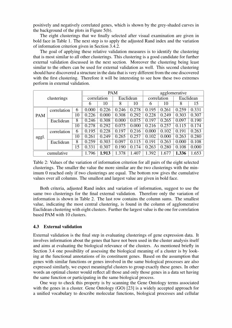
The eight clusterings that we finally selected after visual examination are given inbold face in Table 1. The next step is to apply the adjusted Rand index and the variationof information criterion given in Section 3.4.2.

The goal of applying these relative validation measures is to identify the clusteringthat is most similar to all other clusterings. This clustering is a good candidate for furtherexternal validation discussed in the next section. Moreover the clustering being leastsimilar to the others can be used for external validation as well. This second clusteringshould have discovered a structure in the data that is very different from the one discoveredwith the first clustering. Therefore it will be interesting to see how these two extremesperform in external validation.

PAM agglomerativeclusterings correlation Euclidean correlation Euclidean

6 10 8 10 6 10 8 156 0.000 0.226 0.246 0.278 0.195 0.261 0.259 0.331correlation10 0.226 0.000 0.308 0.292 0.228 0.249 0.303 0.307PAM8 0.246 0.308 0.000 0.075 0.197 0.265 0.097 0.190Euclidean10 0.278 0.292 0.075 0.000 0.216 0.257 0.115 0.1746 0.195 0.228 0.197 0.216 0.000 0.102 0.191 0.263correlation10 0.261 0.249 0.265 0.257 0.102 0.000 0.263 0.280aggl.8 0.259 0.303 0.097 0.115 0.191 0.263 0.000 0.108Euclidean15 0.331 0.307 0.190 0.174 0.263 0.280 0.108 0.000

cumulative 1.796 1.913 1.378 1.407 1.392 1.677 1.336 1.653

Table 2: Values of the variation of information criterion for all pairs of the eight selectedclusterings. The smaller the value the more similar are the two clusterings with the min-imum 0 reached only if two clusterings are equal. The bottom row gives the cumulativevalues over all columns. The smallest and largest value are given in bold face.

Both criteria, adjusted Rand index and variation of information, suggest to use thesame two clusterings for the final external validation. Therefore only the variation ofinformation is shown in Table 2. The last row contains the column sums. The smallestvalue, indicating the most central clustering, is found in the column of agglomerativeEuclidean clustering with eight clusters. Further the largest value is the one for correlationbased PAM with 10 clusters.

4.3 External validation

External validation is the final step in evaluating clusterings of gene expression data. Itinvolves information about the genes that have not been used in the cluster analysis itselfand aims at evaluating the biological relevance of the clusters. As mentioned briefly inSection 3.4 one possibility of assessing the biological meaning of a cluster is by look-ing at the functional annotations of its constituent genes. Based on the assumption thatgenes with similar functions or genes involved in the same biological processes are alsoexpressed similarly, we expect meaningful clusters to group exactly these genes. In otherwords an optimal cluster would reflect all those and only those genes in a data set havingthe same function or participating in the same biological process.

One way to check this property is by scanning the Gene Ontology terms associatedwith the genes in a cluster. Gene Ontology (GO) [23] is a widely accepted approach fora unified vocabulary to describe molecular functions, biological processes and cellular

components of genes or gene products. The terms used for the description of genes andgene products are organized as a directed acyclic graph (DAG) and become more preciseat the lower levels of the graph. It is possible that a single gene has multiple functions,takes part in different processes and appears in several components of the cell. Further,each term in the ontology can have several (less specialized) parent terms and the termsthemselves follow the “true path rule”. This means that a gene product described by achild term is also described by all parent terms.

Many tools exist for accessing the Gene Ontology. For our purpose of evaluating thegenes in a cluster relative to a reference set FatiGO [2] is suitable. It is a web-basedapplication (http://fatigo.bioinfo.cnio.es) that extracts the GO terms for aquery and a reference group of genes and further computes several statistics for the querygroup. We used FatiGO to access the biological process annotations for each cluster Ciin the clusterings selected in the last section. As reference set we used the union of thecorresponding complementary clusters, i. e. all of the clustered genes that do not fall intothis cluster Ci. The GO level to be used in the analysis has to be fixed in advance between2 and 5. We used level 5 because most of the genes under study actually have annotationsat this level7. As a consequence only the subset of a cluster consisting of genes that havelevel 5 annotations can be evaluated this way.

We used two criteria for validating clusters externally. First the cluster selectivity isassessed. This means that the proportion of genes with a certain annotation in the clusterrelative to all genes in the data having this annotation is determined. A high selectivitythus indicates that the clustering algorithm is able to distinguish these genes well, basedon their expression profiles, among all genes.

The second criterion is the cluster sensitivity, the proportion of genes with a certainannotation relative to all genes within the same cluster. If the sensitivity of a cluster ishigh then most genes in the cluster have the same annotation, in this case they participatein the same process. This is important for annotating previously unknown genes. Theputative biological process for an unknown gene found in a very sensitive cluster canbe given with a higher confidence compared to unknown genes in a cluster representinggenes from many different processes.

For the cell cycle data we have selected the two clusterings “agglomerative with Eu-clidean distance and eight clusters” and “PAM with correlation dissimilarity and 10 clus-ters”. It is not possible to give the validation results for each cluster. Rather we give onlyselected results which have some interesting properties.

It must be stated that most clusters are neither very selective nor very sensitive. Thismay be caused on the one hand by using GO annotations from a too high level. Whenthe level is too high, the categories are too coarse so that genes participating in subpro-cesses with rather different expression properties still have the same annotation from thecommon ancestor node in the GO tree. Of course this results in a rather low selectivitybecause the clustering algorithm will not group genes from these subprocesses togetherdue to their different expression profiles. On the other hand when the level is too low,meaning that the annotations are very specific, only few genes actually have a annotationat this level and therefore only a few can have a common annotation. In this case thesensitivity of a cluster is generally low unless the cluster sizes are very small and conse-quently the number of clusters is undesirably large. This shows that there is a trade-offbetween cluster selectivity, sensitivity and the number of clusters.

Figure 6 shows the results of FatiGO8 for Cluster 3 of the hierarchical Euclidean

7Actually almost all genes not being annotated at level 5 have the annotation “molecular function un-known” at level 2.

8Note that the three p-values given in the figure are computed by FatiGO to assess the significance ofthe differences between query and reference set. The first value is the unadjusted p-value, the second and

Figure 6: Part of the output of FatiGO for Cluster 3 of hierarchical Euclidean clusteringwith eight clusters. The six most significant differences between Cluster 3 and the refer-ence set are given. For each GO term the upper bar gives the percentage of genes in thequery cluster and the lower bar in the reference set.

clustering with eight clusters. Cluster 3 contains 25 annotated genes and the referenceset has 134 annotated genes. The figure shows that this cluster is very selective for genesinvolved in protein folding. When looking at the absolute numbers it groups 10 out of 11genes having this annotation. However, it is not very sensitive for protein folding, since60 percent of the cluster is constituted by genes not using this term.

Figure 7: The six most significant differences between Cluster 5 and the reference set forthe same clustering as used in Figure 6.

In Figure 7 Cluster 5, a very sensitive cluster, is shown. Seven of the eight annotatedgenes are labeled with cell organization and biosynthesis. However, it does not have ahigh selectivity for this feature because only 7 out of 45 genes involved in this processhave been selected.

When considering the second clustering, PAM with correlation dissimilarity and 10clusters, the clusters are generally less selective and sensitive, probably caused by thedifferent dissimilarity measure and its properties. Nevertheless for example Cluster 10shown in Figure 8 is both selective and sensitive for protein folding. As in the exampleof Figure 6, it contains 10 out of 11 protein folding genes. But since it is made up by

third value are computed using the false discovery rate adjustment procedure by Benjamini and Hochbergassuming independence and arbitrary dependence between GO terms respectively.

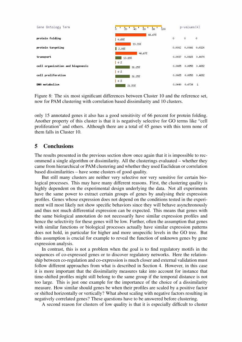
Figure 8: The six most significant differences between Cluster 10 and the reference set,now for PAM clustering with correlation based dissimilarity and 10 clusters.

only 15 annotated genes it also has a good sensitivity of 66 percent for protein folding.Another property of this cluster is that it is negatively selective for GO terms like “cellproliferation” and others. Although there are a total of 45 genes with this term none ofthem falls in Cluster 10.

5 ConclusionsThe results presented in the previous section show once again that it is impossible to rec-ommend a single algorithm or dissimilarity. All the clusterings evaluated – whether theycame from hierarchical or PAM clustering and whether they used Euclidean or correlationbased dissimilarities – have some clusters of good quality.

But still many clusters are neither very selective nor very sensitive for certain bio-logical processes. This may have many different reasons. First, the clustering quality ishighly dependent on the experimental design underlying the data. Not all experimentshave the same power to extract certain groups of genes by analysing their expressionprofiles. Genes whose expression does not depend on the conditions tested in the experi-ment will most likely not show specific behaviors since they will behave asynchronouslyand thus not much differential expression can be expected. This means that genes withthe same biological annotation do not necessarily have similar expression profiles andhence the selectivity for these genes will be low. Further, often the assumption that geneswith similar functions or biological processes actually have similar expression patternsdoes not hold, in particular for higher and more unspecific levels in the GO tree. Butthis assumption is crucial for example to reveal the function of unknown genes by geneexpression analysis.

In contrast, this is not a problem when the goal is to find regulatory motifs in thesequences of co-expressed genes or to discover regulatory networks. Here the relation-ship between co-regulation and co-expression is much closer and external validation mustfollow different approaches from what is described in Section 4. However, in this caseit is more important that the dissimilarity measures take into account for instance thattime-shifted profiles might still belong to the same group if the temporal distance is nottoo large. This is just one example for the importance of the choice of a dissimilaritymeasure. How similar should genes be when their profiles are scaled by a positive factoror shifted horizontally or vertically? What about scaling with negative factors resulting innegatively correlated genes? These questions have to be answered before clustering.

A second reason for clusters of low quality is that it is especially difficult to cluster

microarray data because the expression profiles tend to fill the feature space in a way thatthe data points are not well separated. This leads to the absence of “natural” clusters andclustering becomes segmentation. The known difficulties with the measuring precisionof microarrays are partly overcome by sophisticated normalization methods. Still, theprecision could be greatly improved by repeated measurements at the same conditionsand a better temporal resolution of time series experiments.

The bottom line is that clustering gene expression data from microarrays is a powerfultool in bioinformatics and can reveal biologically relevant information. But it is importantto compare multiple clusterings and not run one algorithm with one parameter setting andthen take the results as the true structure of the data. Only the comparison of carefullychosen clusterings can result in reliable conclusions drawn from cluster analysis.

In this article we have shown how to choose and compare clusterings from differentalgorithms and parameter settings. After selecting meaningful dissimilarity measures a setof candidate clusterings can be chosen by evaluating several internal validation criteria.This includes specifying the number of clusters. Next, relative validation indices can helpto determine the differences between clusterings and identify relatively stable clusters thatappear in several clusterings. These clusters are likely to be more reliable as their structureis extracted from the data by several algorithms or dissimilarity measures. Finally, ifpossible suitable external biological information should be used to assess the quality ofthe clusterings. The Gene Ontology annotations used in this work are of course just oneexample of a source of external information.

However, even conclusions drawn from “good” clusters can only be seen as indica-tions of biological meaning. The power of cluster analysis of gene expression data isthat it can greatly reduce the search space and thus can lead biologists towards promisingpresumptions which are worth further biological examination. The verification of thesepresumptions by biological experiments is not replaceable.

References[1] Chipping Forecast. Nature Genetics Supplement (1999).[2] Al-Shahrour, F.; Diaz-Uriarte, R.; Dopazo, J.: FatiGO: a web tool for finding signif-

icant associations of Gene Ontology terms with groups of genes. Bioinformatics 20(2004) 4, pp. 578–580.

[3] Bolshakova, N.; Azuaje, F.: Cluster validation techniques for genome expressiondata. Signal Processing 83 (2003) 4, pp. 825–833.

[4] Bryan, J.: Problems in gene clustering based on gene expression data. J. Multivari-ate Analysis 90 (2004) 1, pp. 44–66.

[5] Calinski, R. B.; Harabasz, J.: A dendrite method for cluster analysis. Communica-tions in statistics 3 (1974), pp. 1–27.

[6] Cleveland, W. S.; Grosse, E.; Shyu, W. M.: Statistical Models in S, chap. 8.Wadsworth & Brooks/Cole. 1992.

[7] Datta, S.; Datta, S.: Comparisons and validation of statistical clustering techniquesfor microarray gene expression data. Bioinformatics 19 (2003) 4, pp. 459–466.

[8] Eisen, M. B.; Spellman, P. T.; Brown, P. O.; Botstein, D.: Cluster analysis anddisplay of genome-wide expression patterns. Proc. Natl. Acad. Sci. USA 95 (1998),pp. 14863 – 14868.

[9] Gat-Viks, I.; Sharan, R.; Shamir, R.: Scoring clustering solutions by their biologicalrelevance. Bioinformatics 19 (2003) 18, pp. 2381–2389.

[10] Hastie, T.; Tibshirani, R.; Friedman, J.: The Elements of Statistical Learning: DataMining, Inference, and Prediction. Springer. 2001.

[11] Hubert, L.; Arabie, P.: Comparing partitions. Journal of Classification 2 (1985),pp. 193–218.

[12] Jain, A. K.; Dubes, R. C.: Algorithms for clustering data. Prentice-Hall, Inc. 1988.[13] Janowitz, M. F.: Short Course: A Combinatorial Introduction to

Cluster Analysis. Classification Society of North America. URLhttp://www.pitt.edu/˜csna/reports/janowitz.pdf. 2002.

[14] Kaufman, L.; Rousseeuw, P. J.: Finding groups in data. John Wiley & Sons. 1990.[15] Krzanowski, W. J.; Lai, Y. T.: A criterion for determining the number of groups in a

data set using sum of squares clustering. Biometrics 44 (1985), pp. 23–44.[16] Meila, M.: Comparing Clusterings. Tech. Rep. 418, University of Washington.

2002.[17] Milligan, G. W.; Cooper, M. C.: An examination of procedures for determining the

number of clusters in a data set. Psychometrika 50 (1985), pp. 159–179.[18] R Development Core Team: R: A language and environment for statistical

computing. R Foundation for Statistical Computing, Vienna, Austria. URLhttp://www.R-project.org. 2003.

[19] Rand, W. M.: Objective criteria for the evaluation of clustering methods. Journal ofthe American Statistical Association 66 (1971), pp. 846–850.

[20] Rousseeuw, P. J.: Silhouettes: a Graphical Aid to the Interpretation and Validationof Cluster Analysis. Journal of Computational and Applied Mathematics 20 (1987),pp. 53–65.

[21] Spellman, P. T.; Sherlock, G.; Zhang, M. Q.; Iyer, V. R.; Anders, K.; Eisen, M. B.;Brown, P. O.; Botstein, D.; Futcher, B.: Comprehensive Identification of Cell Cycle-regulated Genes of the Yeast Saccharomyces cerevisiae by Microarray Hybridiza-tion. Molecular Biology of the Cell 9 (1998), pp. 3273–3297.

[22] Sturn, A.: Cluster analysis for large scale gene expression studies. Master’s the-sis, Technische Universität Graz and The Institute for Genomic Research (TIGR)Rockville. 2001.

[23] The Gene Ontology Consortium: Gene ontology: tool for the unification of biology.Nature Genetics 25 (2000), pp. 25–29.

[24] Tibshirani, R.; Walther, G.; Botstein, D.; Brown, P.: Cluster validation by predictionstrength. Tech. rep., Stanford University. 2001.

[25] Ward, J. H.: Hierarchical grouping to optimize an objective function. J. Amer.Statist. Assoc. 58 (1963), pp. 236–244.

[26] Wichert, S.; Fokianos, K.; Strimmer, K.: Identifying periodically expressed tran-scripts in microarray time series data. Bioinformatics 20 (2004) 1, pp. 5–20.

[27] Yang, Y. H.: Statistical methods in the design and analysis of gene expression datafrom cDNA microarray experiments. Ph.D. thesis, University of California, Berke-ley. 2002.

[28] Yang, Y. H.; Dudoit, S.; Luu, P.; Lin, D. M.; Peng, V.; Ngai, J.; Speed, T. P.: Nor-malization for cDNA microarray data: a robust composite method addressing singleand multiple slide systematic variation. Nucl. Acids. Res. 30 (2002) 4, pp. e15–.

[29] Zhang, M. Q.: Large-Scale Gene Expression Data Analysis: A New Challenge toComputational Biologists. Genome Research 9 (1999) 8, pp. 681–688.