validating mcnp for leu fuel design via power distribution

ORNL/TM-2008/126

Validating MCNP for LEU Fuel Design via Power Distribution Comparisons

November 2008

D. Chandler R. T. Primm, III G. I. Maldonado

DOCUMENT AVAILABILITY

Reports produced after January 1, 1996, are generally available free via the U.S. Department of Energy (DOE) Information Bridge. Web site http://www.osti.gov/bridge Reports produced before January 1, 1996, may be purchased by members of the public from the following source. National Technical Information Service 5285 Port Royal Road Springfield, VA 22161 Telephone 703-605-6000 (1-800-553-6847) TDD 703-487-4639 Fax 703-605-6900 E-mail [email protected] Web site http://www.ntis.gov/support/ordernowabout.htm

Reports are available to DOE employees, DOE contractors, Energy Technology Data Exchange (ETDE) representatives, and International Nuclear Information System (INIS) representatives from the following source. Office of Scientific and Technical Information P.O. Box 62 Oak Ridge, TN 37831 Telephone 865-576-8401 Fax 865-576-5728 E-mail [email protected] Web site http://www.osti.gov/contact.html

This report was prepared as an account of work sponsored by an agency of the United States Government. Neither the United States Government nor any agency thereof, nor any of their employees, makes any warranty, express or implied, or assumes any legal liability or responsibility for the accuracy, completeness, or usefulness of any information, apparatus, product, or process disclosed, or represents that its use would not infringe privately owned rights. Reference herein to any specific commercial product, process, or service by trade name, trademark, manufacturer, or otherwise, does not necessarily constitute or imply its endorsement, recommendation, or favoring by the United States Government or any agency thereof. The views and opinions of authors expressed herein do not necessarily state or reflect those of the United States Government or any agency thereof.

ORNL/TM-2008/126

Research Reactors Division

VALIDATING MCNP FOR LEU FUEL DESIGN VIA

POWER DISTRIBUTION COMPARISONS

D. Chandler

R. T. Primm, III

G. I. Maldonado

November 2008

Prepared by

OAK RIDGE NATIONAL LABORATORY

Oak Ridge, Tennessee 37831-6283

managed by

UT-BATTELLE, LLC

for the

U.S. DEPARTMENT OF ENERGY

under contract DE-AC05-00OR22725

iii

CONTENTS

Page

LIST OF FIGURES ............................................................................................................................... iv

LIST OF TABLES .................................................................................................................................. v

ABSTRACT ........................................................................................................................................... vi

1. OBJECTIVE .............................................................................................................................. 1

1.1 Motivation ..................................................................................................................... 1

2. INTRODUCTION ..................................................................................................................... 3

2.1 HFIR Description .......................................................................................................... 3

2.2 MCNP5 Description ................................................................................................... 10

2.3 HFIR Cycle 400 MCNP Model .................................................................................. 10

2.4 Critical Experiments ................................................................................................... 18

3. METHODOLOGY .................................................................................................................. 20

3.1 MCNP Changes to Reflect HFIRCE-3 ....................................................................... 20

3.2 Foil Locations ............................................................................................................. 27

3.3 KCODE ....................................................................................................................... 28

3.4 F4 Tallies .................................................................................................................... 29

3.5 Relative Power Density Calculations .......................................................................... 29

4. RESULTS ................................................................................................................................ 33

4.1 Clean Core Conditions ................................................................................................ 33

4.2 Fully Poisoned Core Conditions ................................................................................. 39

5. CONCLUSIONS ..................................................................................................................... 47

6. REFERENCES ........................................................................................................................ 49

Appendix A HFIRCE-3 Data ....................................................................................................... A-1

iv

LIST OF FIGURES

1. HFIR cross section at horizontal midplane ........................................................................... 4

2. Schematic representation of the reactor core ........................................................................ 4

3. HFIR fuel elements ............................................................................................................... 5

4. HFIR flux trap assembly ....................................................................................................... 6

5. HFIR control elements .......................................................................................................... 7

6. HFIR core and beryllium reflector ........................................................................................ 8

7. MCNP model of HFIR cycle 400 at horizontal midplane .................................................. 11

8. Flux trap as loaded in cycle 400 ......................................................................................... 11

9. Involute IFE plate ............................................................................................................... 12

10. IFE 235

U concentration loading and radial modeling .......................................................... 13

11. OFE plate ............................................................................................................................ 14

12. OFE 235

U concentration loading and radial modeling ......................................................... 14

13. Control element dimensions ............................................................................................... 15

14. Control element positions during cycle .............................................................................. 16

15. MCNP model of beryllium reflector at horizontal midplane .............................................. 17

16. MCNP model of radiation barriers ..................................................................................... 17

17. HB-4 as modeled in HFV4.0 .............................................................................................. 21

18. HB-4 as modeled for HFIRCE-3 ........................................................................................ 21

19. HB-2 as modeled in HFV4.0 .............................................................................................. 22

20. HB-2, EF-3, and EF-4 as modeled for HFIRCE-3 .............................................................. 23

21. Horizontal midplane of HFIR as modeled in FHV4.0 ........................................................ 23

22. Horizontal midplane of HFIRCE-3 ..................................................................................... 24

23. Flux trap, fuel elements, and removable beryllium as modeled in HFV4.0 ....................... 25

24. Flux trap, fuel elements, and removable beryllium as modeled for HFIRCE-3 ................. 25

25. (PI+W) flux trap as modeled in MCNP .............................................................................. 26

26. (PI+W) flux trap drawing.................................................................................................... 26

27. Location of foi8ls punched out of removable plates ........................................................... 27

28. Actual versus modeled 235

U concentration of foils in the IFE ............................................ 30

29. Actual versus modeled 235U concentration of foils in the OFE ........................................ 31

30. Radial relative power profile at horizontal midplane under clean core conditions ............. 36

31. Axial relative power profile of foil 1 in IFE under clean core conditions .......................... 36



34. Axial relative power profile of foil 1 in OFE under clean core conditions ......................... 38



37. Radial relative power profile at horizontal midplane under fully poisoned core

conditions ............................................................................................................................ 42

38. Axial relative power profile of foil 1 in IFE under fully positioned core conditions ......... 42

39. Axial relative power profile of foil 4 in IFE under fully poisoned core conditions ............ 43

40. Axial relative power profile of foil 6 in IFE under fully poisoned core conditions ............ 43

41. Axial relative power profile of foil 1 in OFE under fully poisoned core conditions .......... 44



v

LIST OF TABLES

1. Summary of HFIR characteristics ......................................................................................... 9

2. Radial boundaries of core components ................................................................................. 9

3. IFE radial region boundaries ............................................................................................... 13

4. OFE radial region boundaries ............................................................................................. 15

5. Summary of critical experiments ........................................................................................ 18

6. Summary of HFV4.0 and HFIRCE-3 ................................................................................. 20

7. Radial distances to foil’s center from the core axis ............................................................ 28

8. Percent difference of 235

U modeled in IFE.......................................................................... 30

9. Percent difference of 235

U modeled in OFE ........................................................................ 31

10. Average keff, and 68, 95, and 99% confidence intervals for clean core condition .............. 33

11. Experimental and calculated relative power densities under clean core conditions ........... 35

12. Average keff, and 68, 95, and 99% confidence intervals for fully poisoned core

condition .......................................................................................................................... 39

13. Experimental and calculated relative power densities under fully poisoned core

conditions......................................................................................................................... 41

vi

ABSTRACT

The mission of the Reduced Enrichment for Research and Test Reactors (RERTR) Program is to

minimize and, to the extent possible, eliminate the use of highly enriched uranium (HEU) in civilian

nuclear applications by working to convert research and test reactors, as well as radioisotope production

processes, to low enriched uranium (LEU) fuel and targets. Oak Ridge National Lab (ORNL) staff is

reviewing the design bases and key operating criteria including fuel operating parameters, enrichment-

related safety analyses, fuel performance, and fuel fabrication in regard to converting the fuel of the High

Flux Isotope Reactor (HFIR) from HEU to LEU. The purpose of this study is to validate Monte Carlo

methods currently in use for conversion analyses. The methods have been validated for the prediction of

flux values in the reactor target, reflector, and beam tubes, but this study focuses on the prediction of the

power density profile in the core. A current three dimensional (3-D) Monte Carlo N-Particle (MCNP)

model was modified to replicate the HFIR Critical Experiment 3 (HFIRCE-3) core of 1965. In this

experiment, the power profile was determined by counting the gamma activity at selected locations in the

core. “Foils” (chunks of fuel meat and clad) were punched from the fuel elements in HFIRCE-3 following

irradiation and experimental relative power densities were obtained by measuring the activity of these

foils and comparing each foil’s activity to the activity of a normalizing foil. The current work consisted of

calculating corresponding activities by inserting volume tallies into a modified, existing MCNP model to

represent the punchings. The average fission density was calculated for each foil location and then

normalized to the reference foil. Power distributions were obtained for the clean core (no poison in

moderator and symmetrical rod position at 17.5 inches) and fully poisoned-moderator (1.35 g B/liter in

moderator and control elements fully withdrawn) conditions. The observed deviations between the

experimental and calculated values for both conditions were within the reported experimental

uncertainties except for some of the foils located on the top and bottom edges of the fuel plates.

1

1. OBJECTIVE

The purpose of this work is to validate MCNP for implementation of converting the fuel in the HFIR

from HEU to LEU. Monte Carlo methods are currently being utilized for studies including fuel operating

parameters, enrichment-related safety analyses, and fuel performance in regard to converting the fuel of

the HFIR.1 The methods have been validated for the prediction of flux values in the reactor target,

reflector, and beam tubes, but this document focuses on the prediction of the power density profile in the

reactor core.

In order to validate MCNP via power density comparisons, a set of experimentally measured results

are to be utilized. Two data sets of relative power densities that were obtained during the HFIRCE-3

experiments are provided in Tables A.1 and A.2 in ref. 2. The core conditions corresponding to each of

the two experiments are different and therefore provide two unique scenarios to model. The data in Table

A.1 were obtained for a clean core condition in which no boron was present in the moderator and the

control elements were withdrawn at symmetrical positions of approximately 17.5 inches relative to the

core axial midplane. This configuration corresponds to reactor startup. The set of data listed in Table A.2

were measured under fully poisoned core conditions in which 1.35 grams of boron per liter of moderator

was present and the control elements were fully withdrawn. This configuration corresponds to the end-of-

life conditions in the reactor with the uranium loss during the cycle and the poisoning effect of fission

products approximated by the addition of boron to the coolant.

The first objective of this study is to develop a 3-D model that replicates the HFIRCE-3 experiment

configuration. This will be done by modifying the HFV4.0 model, which is a 3-D MCNP model that

replicates HFIR as loaded in cycle 400.3 The next step is to utilize this modified model of the HFIRCE-3

reactor configuration to compute the relative power density of each foil. Finally, the computational results

are to be compared to the experimental results.

1.1 MOTIVATION

The Reduced Enrichment for Research and Test Reactors (RERTR) program was established with the

intent of minimizing and, to the extent possible, eliminating the use of HEU in civilian nuclear

applications by working to convert research and test reactors and radioisotope production processes to the

use of LEU fuel and targets throughout the world. Below is a list of the key analyses needed to be

performed before converting from HEU to LEU fuel:

1. ensure that the ability of the reactor to perform its scientific mission is not significantly

diminished,

2. work to ensure that an LEU fuel alternative is provided that maintains a similar service lifetime

for the fuel assembly,

3. ensure that conversion to a suitable LEU fuel can be achieved without requiring major changes in

reactor structures or equipment,

4. determine, to the extent possible, that the overall costs associated with conversion to LEU fuel

does not increase the annual operating expenditure for the owner/operator, and

5. demonstrate that the conversion and subsequent operation can be accomplished safely and the

LEU fuel meets safety requirements.

Experiments and expert-based opinions were used in order to finalize the design for the current HFIR

production core. Today however, numerical analysis programs are available and are able to accurately

predict pertinent physics parameters, and are thus utilized for studies such as converting to LEU fuel.

Additionally, utilizing computationally based programs is useful and economical for safety assessments in

which it is undesirable to experimentally determine the transient behavior of the reactor and similarly, to

minimize the risk of failure of a specimen proposed for irradiation and the consequences of such a failure

should it occur. For design and safety purposes, it is vital to validate computer codes before relying on

their results, and thus is the basis of this report.

2

In order to convert the HFIR core from HEU to LEU without changing the geometry of the core, the

fuel must be much denser and, therefore, metallic rather than ceramic. This change can easily be modeled

by modifying the atom densities in the fuel elements in HFV4.0 or the models created in this study. The

determination of the required modification (new atom densities) is not performed or documented in this

study, but is the basis of other studies currently being performed at ORNL.

In the past, diffusion codes such as BOLD VENTURE and DORT have been used to calculate power

densities in the reactor core, but these models were, of necessity, approximations to the core geometry

and 2-D. 3-D diffusion codes have been used, but only power profiles calculated from 2-D diffusion

codes have been documented. Also, all of the previous power density calculations have been compared to

data fitted from the measured results reported in Tables A.1 and A.2 in ref. 2. This study focuses on using

a transport code rather than a diffusion code, using a detailed 3-D geometry of the reactor rather than a

less complex 2-D geometry, and calculating power densities to be directly compared to the measured

results rather than to data interpolated and extrapolated from these measured values.

3

2. INTRODUCTION

A detailed 3-D MCNP model (HFV4.0) has previously been developed to accurately represent the

HFIR as loaded in cycle 400.3 HFV4.0 was developed in order to accurately predict data such as the

reactivity worth and heat generation rate of specimens to be irradiated in the reactor. In the past, direct

measurements and expert-based opinions were the primary source of this data, but now, numerical

analysis programs are available and are able to better predict these physics parameters, especially for

novel applications of reactor facilities. Additionally, utilizing computational estimates is required for

safety assessments in which it is undesirable to experimentally determine the transient behavior of the

reactor due to specimen irradiation and similarly, to minimize the risk of failure of a specimen proposed

for irradiation and the consequences of such a failure should it occur.

Currently, a great deal of research is going on at HFIR, such as converting the fuel from HEU to

LEU, extending the cycle length from 23 days to beyond 30 days, and increasing the power from 85 MW

to 100 MW. Converting to LEU will increase the total amount of fuel in the core from 10 kg of HEU to

approximately 130 kg of LEU. To accomplish this increase, it will be necessary to increase the density of

the fuel by using metallic fuel rather than ceramic fuel. This document was written for the purpose of

validating Monte Carlo methods which are being used in the design of an LEU fuel cycle. The methods

and the model had been validated for the prediction of flux values in the reactor, target region, and

reflector4 but had never been validated for the prediction of the power density profile in the reactor core.

The HFV4.0 model is to be modified in order to accurately replicate the HFIR configuration during

Critical Experiment 3 (HFIRCE-3).

Relative power densities are to be computed and compared to the experimental results collected in the

fall of 1965. Previous calculations have been performed with other computational methods (deterministic

methods) in order to compare calculated power distributions to the power distribution profiles

interpolated and extrapolated from data measured during the critical experiments in 1965.5 The

calculation-to-experiment differences found in those studies were greater than the reported uncertainties

in the experimental measurements for many locations in the reactor core. The Monte Carlo method,

examined here, coupled with point energy data for neutron cross sections, should provide the most

accurate computational model possible of the critical experiments. The reported, calculated, relative

power distributions were derived such that they could be compared to the data directly measured in the

critical experiments.

2.1 HFIR DESCRIPTION

The High Flux Isotope Reactor is a multipurpose isotope production and test reactor with a rated

power of 100 MW (currently operating at 85 MW) and the capability of performing a variety of

irradiation experiments. The HFIR first achieved criticality on August 25, 1965. This versatile flux-trap

reactor had (and still has with its decrease in power) the highest neutron flux in the western world with a

peak thermal-neutron flux in the flux trap of 5.5 x 1015

neutrons/cm2•s at its maximum steady-state power

of 100 MW. HFIR was originally designed primarily for producing transplutonium isotopes. Plutonium-

242 and heavier recycle materials are placed in the central flux trap and are irradiated in order to produce

californium-252 and other lighter transplutonium isotopes. Besides the flux trap, numerous other

experimental facilities such as the removable beryllium facilities, control rod access plug facilities, and

the vertical experiment facilities are used for isotope production. A horizontal and a vertical depiction of

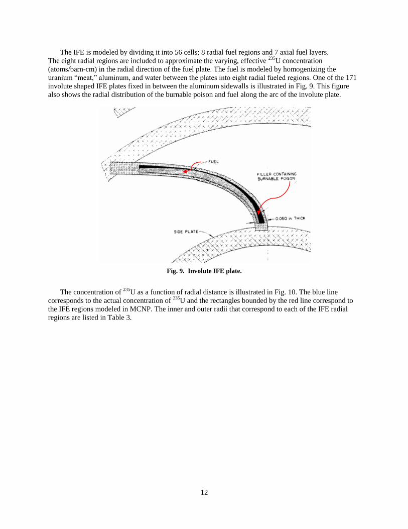
HFIR are illustrated in Fig. 1 and Fig. 2 respectively.

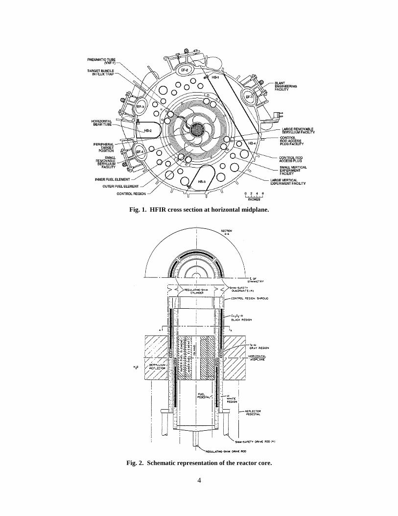
4

Fig. 1. HFIR cross section at horizontal midplane.

Fig. 2. Schematic representation of the reactor core.

5

Following a shutdown at the end of 1986, pressure vessel embrittlement was assessed and questions

about procedural adequacy were answered. The reactor was then restarted in January of 1990 at a power

level of 85 MW. Still, at 85 MW, HFIR is capable of a peak thermal neutron flux of 2.6 x 1015

neutrons/cm2•s. Today HFIR has three main purposes. Besides producing isotopes such as californium-

252, the reactor provides neutron activation analysis and neutron scattering capabilities. Neutron

scattering is the primary purpose of HFIR today and is used to study the molecular and magnetic behavior

and structure of materials such as high-temperature superconductors, polymers, metals, and biological

samples.

HFIR is a beryllium-reflected, light water-cooled and moderated, pressurized flux-trap type reactor

that utilizes highly enriched (~93%) uranium fuel. HFIR isn’t used to generate electricity, and the heat

created is dissipated through heat exchangers to a cooling tower. The reactor core consists of two

concentric annular regions labeled as the Inner Fuel Element (IFE) and the Outer Fuel Element (OFE).

The IFE contains 171 involute-shaped fuel plates and the OFE contains 369 involute-shaped fuel plates,

which are all held in place by aluminum side walls. The HFIR fuel elements are depicted in Fig. 3. The

fuel consists of U3O8-Al cermet with aluminum clad, which is nonuniformly distributed along the arc of

the involute to minimize the radial peak-to-average power density ratio. A single IFE and OFE fuel plate

contains approximately 15.18 and 18.44 grams of 235

U respectively, which yields a total core loading of

9.4 kilograms of 235

U. The IFE also contains 2.8 grams of 10

B which is primarily used to shift the power

distribution from the IFE to the OFE. With this fuel, the average core life varies between 19 and 26 days

depending on the amount and type of material being irradiated.

Fig. 3. HFIR fuel elements.

6

A cylindrical cavity is located in the center of the core and is referred to as the flux trap. The flux trap

consists of 37 experimental sites; 31 of these sites are located in the interior of a basket; the other 6 are

located on the periphery of the basket and are referred to as the peripheral target positions (PTPs). One of

the interior sites is connected to a hydraulic tube that allows for the insertion and removal of capsules.

These capsules are irradiated for a short duration (minutes to hours) and are typically utilized for medical

isotope production. The other interior positions are typically occupied by target rods used for the

production of transplutonium elements. The PTPs, located at the outer radial edge of the flux trap where

the highest fast-neutron flux exists, are primarily used for materials irradiation studies. The thermal

neutron flux in the flux trap is primarily due to the moderation in the trap of high energy neutrons that

leak out of the fuel region. A mockup of the flux trap, as well as the IFE and OFE is shown in Fig. 4.

Fig. 4. HFIR flux trap assembly.

Two poison-bearing concentric control plates are located between the OFE and the beryllium

reflector. The inner control plate consists of one thin cylindrical tube and is used for shimming and

regulation and thus not used for a fast safety function. The outer control plate consists of four separate

quadrants, each having an independent drive and safety release mechanism. Each of the control plates has

three regions of different poison content. The top and bottom of the control plates known as the white

region are composed of aluminum and provide flow (they are perforated) and structural stability. The grey

region is made up of tantalum-aluminum (Ta-Al) which is a moderately absorbing material and the black

region is composed of europium oxide-aluminum (Eu2O3-Al) which is a strong neutron absorber. The

inner control element cylinder and one of the outer control element quadrants are shown in Fig. 5. During

the course of starting the reactor, the inner control plate is driven downward (driving the black region

away from the core) and the outer control plate driven upward (also driving the black region away from

the core). Thus, positive reactivity is inserted as the plates are driven in opposite directions. The drive

mechanisms are located under the pressure vessel in a sub-pile room, which provides shielding to workers

below the core and access to the pressure vessel, reactor core, and reflector regions.

7

Fig. 5. HFIR control elements.

On the outside of the fuel region and the control blades is a concentric ring of beryllium reflector,

which is composed of a removable reflector, a semi-permanent reflector, and a permanent reflector, as

illustrated in Fig. 6. As the name suggests, the function of the beryllium reflector is to reflect the neutrons

that leak out of the fuel region back into the fuel region. Four small removable beryllium facilities (small

RB) and eight large removable beryllium facilities (large RB) are located in the removable beryllium

region and are used primarily for the production of radioisotopes. Four control rod access plug facilities

(CRAP) are located in the semi-permanent beryllium reflector and are also used for isotope production.

Sixteen small vertical experiment facilities (VXF) and six large vertical experiment facilities penetrate the

permanent reflector and normally un-instrumented experiments are irradiated in these facilities. Water of

effectively infinite thickness is located on the outside of the beryllium reflector, as well as above and

below the reactor and within the pressure vessel walls.

8

Fig. 6. HFIR core and beryllium reflector.

The beamlines supply neutrons to a wide variety of instruments including HB-1 (Polarized Triple-

Axis Spectrometer), HB-1A (Fixed Incident Energy Triple-Axis Spectrometer), HB-2A (Neutron Powder

Diffractometer), HB-2B (NRS2 – Neutron Residual Stress Mapping Facility), HB-2C (Wand - U.S. –

Japan Wide Angle Neutron Diffractometer), HB-3 (Triple Axis Spectrometer), HB-3A (Single-Crystal

Four-Circle Diffractometer), CG-2(Small Angle Neutron Scattering Diffractometer), CG-3(BIO-SANS –

Biological Small-Angle Neutron Scattering Instrument), and CG-4C (U.S. – Japan Cold Neutron Triple

Axis Spectrometer). HFIR is equipped with four horizontal beam tubes that extend outward from the

reactor core at the midplane and through the pool wall. HB-2 extends radially from the reactor’s vertical

centerline, with its inner end penetrating the permanent reflector. HB-3 extends tangentially from the core

(approximately 10 ½ inches from the vertical centerline), and like HB-2, penetrates the permanent

reflector. HB-1 and HB-4 are aligned on a tangential line approximately 15 1/8 inches away from the

vertical centerline and are separated by beryllium. Two slant engineering facilities (SEF) provide

additional neutron beams for experiments and are inclined 49° from the horizontal. The inner end of a

SEF terminates at the outer periphery of the Be reflector and the upper end terminates at the outer face of

the pool wall in an experiment room. Fig. 1 provides a schematic illustration of the HFIR horizontal

midplane, and shows the location of the four horizontal beam tubes.

Two other experimental facilities at HFIR include the neutron activation analysis lab (NAA) and the

gamma irradiation facility (GIF). Some of the applications of NAA at HFIR include nuclear

nonproliferation, forensics, ultra-trace metrology, environmental, isotope production, and materials

irradiation. Sample irradiation and environmental qualification of materials used in radioactive fields are

performed in the GIF by lowering the specimen into the HFIR pool and irradiating it with the gamma flux

generated from the decay of fission products from the spent fuel.

A summary of the HFIR characteristics including fuel specifications are listed in Table 1 and the

radial dimensions (cylindrical boundaries) of the core components of the reactor are listed in Table 2.

9

Table 1. Summary of HFIR characteristics

Parameter Units Value

Reactor Power MW 85

Maximum Thermal Neutron Flux neutrons/cm2•s 2.6 x 10

15

Active Core Height cm 50.8

Number of Fuel Elements - 2

Fuel Type - U3O8-Al

Total 235

U Loading kg 9.40

Enrichment % 235

U 93

Fuel Element - IFE OFE

Number of Fuel Plates - 171 369 235

U per Plate g 15.18 18.44

Average Fuel U Density gU/cm3 0.776 1.151

235U Loading kg 2.60 6.80

Burnable Poison in Element g 10

B 2.8 0

Fuel Plate Thickness cm 0.127 0.127

Coolant Channel Between Plates cm 0.127 0.127

Minimum Al Clad Thickness mm 0.25 0.25

Fuel Plate Width cm 8.1 7.3

Coolant and Moderator - H2O

Fuel Cycle Length days 19-26

Coolant Inlet Temperature °F 120

Coolant Outlet Temperature °F 169

Fuel Plate Centerline Temperature °F 323

Table 2. Radial boundaries of core components

Region Inner Radius (cm) Outer Radius (cm)

Flux Trap 0 6.43

IFE Side Plate 6.43 13.45

IFE Active Element 7.14 12.60

OFE Side Plate 14.29 21.76

OFE Active Element 15.13 20.98

Control Elements 21.76 23.97

Removable Reflector 23.97 30.17

Permanent Reflector 30.17 54.61

Water Reflector 54.61 119.38

Pressure Vessel 119.38 121.92

10

2.2 MCNP5 DESCRIPTION

MCNP is a three-dimensional general-purpose code that was developed and is maintained by Los

Alamos National Laboratory (LANL).6 MCNP can be used to simulate neutron, photon, electron, or

coupled neutron/photon/electron transport. MCNP is typically used in areas such as nuclear criticality

safety, fission and fusion reactor design, decontamination and decommissioning, radiation

protection/shielding, dosimetry, radiography, and medical physics.

MCNP utilizes three-dimensional geometry and has powerful source modeling capabilities. The code

treats an arbitrary three-dimensional configuration of materials in geometric cells bounded by first- and

second-degree surfaces and fourth-degree elliptical tori. Or more simply, three-dimensional objects are

constructed by bounding the surfaces of the cell while filling the cell with the appropriate material.

The latest version of MCNP, MCNP5, is used throughout this study. The geometry of the HFIR was

modeled in MCNP and volume tallies were inserted into the fuel elements such that the average fission

densities (fissions/cm3) could be calculated. Continuous energy cross section data from ENDF/B-VI are

used with MCNP in this study.

The Visual Editor code, which is part of the MCNP5 package, was used for assistance in the creation

of MCNP input files. Visual Editor reads the MCNP input file and displays cross sectional views of the

model.

2.3 HFIR CYCLE 400 MCNP MODEL

The 3-D MCNP model, HFV4.0, accurately represents the HFIR as loaded in cycle 400 (see Fig. 7).

HFV4.0 is based on an older model that was previously developed at ORNL and was documented in

ref. 3. The model is set up such that the user can modify the input cards to reflect any changes to the

model or future experimental rearrangements such as the flux trap loading. Continuous energy neutron

ENDF/B-VI cross-section data libraries are utilized in the model. The MCNP model is broken up into six

regions (parts), as follows:

Region 1: Flux Trap Target Region (FTT)

Region 2: Inner Fuel Element Region (IFE)

Region 3: Outer Fuel Element Region (OFE)

Region 4: Control Element Region (CE)

Region 5: Removable Beryllium Reflector Region (RB)

Region 6: Permanent Beryllium Reflector Region

11

Fig. 7. MCNP model of HFIR cycle 400 at horizontal midplane.

The FTT consists of 37 experimental sites; 31 of these sites are located in the interior of the basket

and the other 6 are located on the periphery of the basket and are referred to as the peripheral target

positions (PTPs). Refer to Fig. 8 for the flux trap loading of cycle 400. The cycle 400 loading consists of

7 solid aluminum dummy targets (orange regions), 21 shrouded aluminum dummy targets (pink with

green rings surrounded by blue annuli), 2 stainless steel targets (solid light pink), 1 hydraulic tube

(containing green, pink, and green concentric annuli), and 6 PTP tubes (different colors located on the

periphery at 60° intervals).

Fig. 8. Flux trap target as loaded in cycle 400.

12

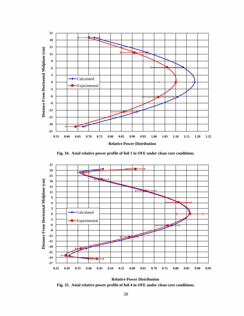
The IFE is modeled by dividing it into 56 cells; 8 radial fuel regions and 7 axial fuel layers.

The eight radial regions are included to approximate the varying, effective 235

U concentration

(atoms/barn-cm) in the radial direction of the fuel plate. The fuel is modeled by homogenizing the

uranium “meat,” aluminum, and water between the plates into eight radial fueled regions. One of the 171

involute shaped IFE plates fixed in between the aluminum sidewalls is illustrated in Fig. 9. This figure

also shows the radial distribution of the burnable poison and fuel along the arc of the involute plate.

Fig. 9. Involute IFE plate.

The concentration of 235

U as a function of radial distance is illustrated in Fig. 10. The blue line

corresponds to the actual concentration of 235

U and the rectangles bounded by the red line correspond to

the IFE regions modeled in MCNP. The inner and outer radii that correspond to each of the IFE radial

regions are listed in Table 3.

13

Fig. 10. IFE

235U concentration loading and radial modeling.

Table 3. IFE radial region boundaries

Radial Fueled Region Inner Radius (cm) Outer Radius (cm)

1 7.14 7.50

2 7.50 8.00

3 8.00 8.50

4 8.50 9.50

5 9.50 10.50

6 10.50 11.50

7 11.50 12.00

8 12.00 12.60

The OFE is modeled by dividing it into 63 cells; 9 radial fueled regions, and 7 axial fueled layers. The

nine radial regions represent the different effective 235

U concentrations (atoms/barn-cm) in the radial

direction of the fuel plate. One of the 369 involute shaped OFE plates fixed in between the aluminum

sidewalls is depicted in Fig. 11, and a plot that represents the concentration of 235

U as a function of radial

distance in an OFE plate is shown in Fig. 12. The blue line corresponds to the actual concentration of 235

U

and the rectangles bounded by the red line correspond to the OFE regions modeled in MCNP. The inner

and outer radii that correspond to each of the OFE radial regions are listed in Table 4.

14

Fig. 11. OFE plate.

Fig. 12. OFE

235U concentration loading and radial modeling.

15

Table 4. OFE radial region boundaries

Radial Fueled Region Inner Radius (cm) Outer Radius (cm)

1 15.13 15.50

2 15.50 16.00

3 16.00 16.50

4 16.50 17.50

5 17.50 18.50

6 18.50 19.50

7 19.50 20.00

8 20.00 20.50

9 20.50 20.98

The control element region (CE) consists of two thin-walled (0.25-in.) concentric cylindrical zones.

The inner control element and outer control elements are both composed of three axial regions. The top

and bottom of the control plates known as the white region are composed of aluminum. The grey region is

made up of tantalum-aluminum (Ta-Al), and the black region is composed of europium oxide-aluminum

(Eu2O3-Al). Gaps between the four quadrants in the outer safety element are explicitly modeled, and the

“flow holes” in the control elements are homogenized. The layout and dimensions of the control elements

are shown in Fig. 13 and the positions of the control elements during various stages throughout the cycle

are illustrated in Fig. 14.

Fig. 13. Control element dimensions.

16

Fig. 14. Control element positions during cycle.

The composition of the beryllium in all of the reflectors is the same; however the presence of cooling

water channels causes homogenized atom densities for the three reflector regions to differ. Twenty

experiment facilities are located in this region and include:

eight large RB positions designated in pairs, e.g., RB1 and RB1*, located in the removable

beryllium zone,

four small RB positions located in the semi-permanent beryllium reflector, and

eight control-rod access plug (CRAP) facilities located in the semi-permanent beryllium reflector.

The permanent beryllium reflector extends approximately 20 cm beyond the outside radius of the

semi-permanent reflector. It is surrounded by approximately 50 cm of water and then the steel pressure

vessel. The permanent beryllium includes:

six large VXFs,

eleven inner small VXFs,

five outer small VXFs,

two engineering facilities (vertical slant tubes),

HB-1/HB-4 through tube,

HB-2 radial beam tube, and

HB-3 tangential beam tube.

Equilibrium poisons (Li-6 and He-3) resulting from fast neutron reactions in beryllium are modeled in a

zone-wise fashion in the reflector.

The beryllium reflector, as modeled in MCNP, is illustrated in Fig. 15. This figure represents the

horizontal midplane of the reflector and illustrates the locations of the above experimental facilities. See

Fig. 1 for the schematic illustration of the reactor core horizontal midplane with all of the facilities

labeled.

17

Fig. 15. MCNP model of beryllium reflector at horizontal midplane.

On the outside of the permanent beryllium reflector is approximately 50 cm of water (blue in Fig. 16).

On the outside of the water is the steel pressure vessel and concrete (peach in Fig. 16). The pink area in

Fig. 16 represents an outside void, i.e. reactor structures are not modeled in this region.

Fig. 16. MCNP model of radiation barriers.

18

2.4 CRITICAL EXPERIMENTS

During the early stages of HFIR, four sets of critical experiments were conducted. The first critical

experiment, HFIRCE-1, was performed in order to explore the basic characteristics of the flux trap

geometry. The second critical experiment, HFIRCE-2, included a full mockup of the core essentials and

data including power distributions, control-rod integral and differential worths, shutdown margins,

temperature coefficients, void coefficients, fuel coefficients, neutron lifetimes, worths of simulated

plutonium targets, flux distributions, and worth of beam tube flooding was measured and calculated.

From this experiment, it was concluded that the amount of 235

U was to be increased from 8.01 kg to 9.4

kg and the radial distributions of the fuel and burnable poisons were also to be altered. The third

experiment, HFIRCE-3, was conducted because of some concern over having the ability to extrapolate

with sufficient accuracy from the second critical experiment to the final design. The HFIRCE-3

components were essentially the same as the production components, and the information obtained from

this set of experiments was similar to that obtained by HFIRCE-2 minus the temperature and void

reactivity coefficients and the worth of beam tube flooding. The fourth set of experiments, HFIRCE-4,

was conducted primarily to verify that adequate simulations existed between the critical facility and the

reactor facility. No changes resulted from these experiments.

The HFIRCE-2 fuel elements contained 8.01 kg of 235

U and the inner fuel element contained 1.7 g 10

B. Aluminum, nickel, and silver-copper were used for the white, grey, and black regions of the control

elements, respectively. Nickel, however, has a large scattering cross section, and was therefore rejected as

the grey region. The second set of control elements utilized in HFIRCE-2 was the same as the previous,

except that the nickel region was replaced by a silver-aluminum region. As discussed above, the amount

of 235

U was increased to 9.4 kg from HFIRCE-2 to HFIRCE-3, and therefore the amount of boron

increased from 1.7 g 10

B to 2.12 g 10

B. Due to the increase in 235

U and 10

B, the distribution of the fuel and

poison along the arc on the involute fuel plates had to be changed. The 10

B loading in the IFE of the

HFIRCE-3 core was originally 2.12 g, but was eventually increased to 3.60 g before decreasing to 2.80 g.

The 10

B loading was decreased from 3.60 g to 2.80 g because of the introduction of the tantalum-

aluminum (Ta-Al) and europium oxide-aluminum (Eu2O3-Al) control elements which have a larger worth

than the Ag-Al and Ag-Cu elements. A summary of the 235

U and 10

B loadings, as well of the control

elements utilized in the critical experiments are listed in Table 5.

Table 5. Summary of critical experiments

Experiment ~ 235

U Loading (kg) 10

B Loadinga (g) Control Elements

b

CE-2 8.01 1.7 Al, Ni, Ag-Cu

CE-2 8.01 1.7 Al, Ag-Al, Ag-Cu

CE-3 9.40 2.12 Al, Ag-Al, Ag-Cu

CE-3 9.40 3.60 Al, Ag-Al, Ag-Cu

CE-3c 9.40 2.80 Al, Ta-Al, Eu2O3-Al

CE-4 9.40 2.80 Al, Ta-Al, Eu2O3-Al

Today 9.40 2.80 Al, Ta-Al, Eu2O3-Al

a Only in Inner Fuel Element

b In the form white, grey, black regions

c The basis of this study

In order to obtain the relative power distributions, some removable fuel plates of the same fuel and

poison loading were inserted in place of some of the fixed plates in the IFE and OFE. Chunks of the fuel

meat and clad were punched from the plates and were then reinserted into the plate. These chunks are

referred to as foils in ref. 2 and will be referred to as foils in this report. The foils were punched out of the

plates in order to measure the fission densities which would eventually be converted to and documented

19

as the relative power densities. The locations and dimensions of the foils are depicted in Fig. 27 of

Section 3.2. Three foils are distributed axially along the inner edge, center, and outer edge in order to

obtain a 2-D power distribution. Since the axial midplane is expected to have the highest power density,

six foils were punched at the axial center of the plate in order to better obtain a representation of the

power distribution at the center. Up to six plates in each element were used, but due to the symmetry of

the core, it was determined that only three plates in each fuel element were necessary to obtain

satisfactory power distribution data. The fuel plates were located in positions such that the perturbations

associated with the beam tubes, longitudinal gaps in the control elements, and other irradiation facilities

could be analyzed. From these experiments, it was determined that the beam tubes had essentially no

impact on the power distribution and the circumferential locations 97a in the IFE and 207b in the OFE

constituted the best average removable plate locations. Refer to Fig. A3 in the Appendix for the locations

of these plates. Power distributions were obtained for different control rod positions, different poisoned

moderator conditions, and different flux trap loadings.

Before the removable plates and foils were inserted into the core and irradiated, the foils were

counted in a scintillation counter, and the weight of 235

U was determined. After irradiation, the foils were

counted in a high pressure well-type gamma ionization chamber. The relative power densities were

obtained by comparing the total gamma activity of each of the foils with the time interpolated activity of a

normalizing foil that had been irradiated at the same time and was counted periodically during the

counting of the other foils.

20

3. METHODOLOGY

3.1 MCNP CHANGES TO REFLECT HFIRCE-3

In order to accurately reproduce the power distribution data from HFIRCE-3, it is necessary to first

modify the current MCNP model, HFV4.0, to replicate the core and components as they were during

HFIRCE-3. The main differences (and some similarities) between the cycle 400 production core and

HFIRCE-3 core are listed in Table 6.

Table 6. Summary of HFV4.0 and HFIRCE-3

HFV4.0 HFIRCE-3

2.80 g 10

B Loading in IFE 2.80 g 10

B Loading in IFE

9.40 kg 235

U 9.40 kg 235

U

Target Bundle in Flux Trap (Plastic Island + Water) in Flux Trap

HB-2 was Enlarged and Upgraded HB-2 was of Nominal Size

2 Engineering Facilities (Slant Tubes) 4 Engineering Facilities (Slant Tubes)

HB-4 was Enlarged and Cold Source Inserted HB-4 was of Nominal Size

8 Large Removable Beryllium Facilities 4 Large Removable Beryllium Facilities

Pressurized Open to Atmosphere

Water Flow to Remove Heat Stagnant Flow

85 MW Essentially Zero Power

At the time of the critical experiments, there were three horizontal beam tubes with 10.16 cm inner

diameter that extended outward from the reactor core at the midplane (HB-2, HB-3, and HB-1/HB-4).

HB-2 extends radially from the reactor’s vertical centerline with its inner end penetrating the permanent

beryllium reflector. HB-3 extends tangentially from the core, offset approximately 26.67 cm from the

reactor’s vertical centerline and also penetrates the permanent reflector. Also, a through tube with

designated ends of HB-1 and HB-4 is a tube that is aligned on a tangential line approximately 38.42 cm

from the reactor’s vertical centerline and is separated by beryllium, which in the model is assumed to be

of the same composition as the beryllium reflector in that area.

HB-4 was originally designed as a 30-m small angle neutron scattering facility as a tool for the

characterization of long-range fluctuations in scattering density, as well as materials science and

engineering, solid state physics, polymer research, and the biological sciences. During the six month

outage that began in May of 2000, HB-4 was enlarged and, later, in 2007, transformed into a high

performance hydrogen cold source. The cold source is used to slow down the neutron beam and thus,

decrease the beam’s energy. HB-4 as modeled in MCNP for cycle 400, which includes the cold source, is

depicted in Fig. 17, and HB-4 as modeled in the critical experiments is depicted in Fig. 18.

21

Fig. 17. HB-4 as modeled in HFV4.0.

Fig. 18. HB-4 as modeled for HFIRCE-3.

22

HB-2, originally a triple-axis spectrometer, was also enlarged and altered during the outage that

ended in 2000, and now supports a neutron powder diffractometer, a neutron residual stress mapping

facility, and a wide angle neutron diffractometer. During the enlargement of HB-2, two of the four slant

engineering facilities were eliminated. The slant engineering facilities are located about the periphery of

the beryllium reflector and were designed to accommodate experiments that require relatively low

neutron fluxes. The slant facilities are 10.16 cm OD tubes that enter the pressure vessel at an elevation of

251.5 m, extend downward at an angle of about 41°, and terminate at the outer face of the pool wall in the

experiment room. An x-y cross section of HB-2 as modeled in cycle 400 is illustrated in Fig. 19, and HB-

2 as modeled in HFIRCE-3 is shown in Fig. 20. Fig. 20 illustrates the locations of EF-3 and EF-4 before

they were removed during the enlargement of HB-2, which is illustrated in Fig. 19. Fig. 21 and Fig. 22

better show these changes with a “zoomed out” view of the reactor core, reflector, and pool at the

horizontal midplane.

Fig. 19. HB-2 as modeled in HFV4.0.

23

Fig. 20. HB-2, EF-3, and EF-4 as modeled for HFIRCE-3.

Fig. 21. Horizontal midplane of HFIR as modeled in HFV4.0.

24

Fig. 22. Horizontal midplane of HFIRCE-3.

The number of large removable beryllium (RB) facilities was increased from the original number of

four to eight. The four original large RB facilities (RB-1, RB-3, RB-5, and RB-7) were installed in the

removable beryllium reflector located 27.31 cm from the vertical centerline of the reactor. The large RB

facilities have an aluminum liner with an inner diameter of 3.56 cm and have been primarily utilized for

HTGR fuel irradiations and the production of isotopes. When these facilities aren’t occupied for

experimental purposes, beryllium plugs are inserted into the facility. Recently, four more large RB

facilities were installed and are located next to the original facilities such that they are grouped in pairs at

90° intervals. The facilities are now designated as RB-1A and RB-1B, RB-3A and RB-3B, RB-5A and

RB-5B, and RB-7A and RB-7B. For the cycle 400 loading, RB-1A was loaded with an aluminum target,

and the liner and target loading of RB-7A was europium. Thus, these materials were changed in the

MCNP model such that an aluminum liner and a beryllium plug were modeled. The increase of large RB

facilities can be viewed by comparing Fig. 23 to Fig. 24. These figures also show the change in the flux

trap as viewed at the horizontal midplane.

25

Fig. 23. Flux trap, fuel elements, and removable beryllium as modeled in HFV4.0.

Fig. 24. Flux trap, fuel elements, and removable beryllium as modeled for HFIRCE-3.

26

During the critical experiments, a flux trap target referred to as a plastic island filled with water (PI

+W) flux trap was utilized. The (PI + W) flux trap consisted of a polyethylene insert that was located

within an aluminum tube, which sat on top of a stainless steel sinker plate. The polyethylene target was

either a solid polyethylene target or filled with water. The original drawing of the (PI +W) flux trap is

illustrated in Fig. 26, and the y-z plane of the MCNP model of the (PI +W) flux trap is depicted in Fig.

25. The central (neon green) area in Fig. 25 is the water region, the blue region is the polyethylene insert,

the red top and bottom regions represent the aluminum tube lifting plate and the aluminum end plate, and

the light blue area at the bottom of the flux trap is the steel sinker plate. An important point to notice is

that the diameter of the water region is greater in Fig. 25 than the water region in Fig. 26. Two (PI + W)

flux traps were designed; one with a 9.287 cm (3 21/32 inch) diameter and one with a 6.191 cm (2 7/16

inch) diameter. The flux trap in Fig. 25 includes the 9.287 cm diameter water gap and the flux trap in Fig.

26 includes the 6.191 cm diameter water gap. Since it is unclear which flux trap was used, both diameters

were analyzed. The deviation between calculated k-effectives for the two configurations was statistically

insignificant.

Fig. 25. (PI +W) flux trap as modeled in MCNP.

Fig. 26. (PI +W) flux trap drawing.

27

3.2 FOIL LOCATIONS

A schematic of a removable plate is illustrated in Fig. 27 and shows the placement of the removable

foils that were previously described. Since the plates are symmetric about the vertical centerline, only half

of the plate is shown. The foils that are located below the centerline are suffixed with the letters E, F, G,

HH, and H. Note that the drawing is not to scale and the dimensions are recorded in centimeters. Also, the

dimensions correspond to the axial height and the arc distance from the involute generating circle rather

than the radial distance from the side walls. The radial distances between the core centerline and the

center of the foils for both the inner and outer fuel elements are listed in Table 7.

Fig. 27. Location of foils punched out of removable plates.

28

Table 7. Radial distances to foil's center from the core axis

Foil ρ(cm), IFE ρ(cm), OFE

1 7.38632 15.38986

2 8.40232 16.46936

3 9.41832 17.54886

4 10.43432 18.62836

5 11.45032 19.70786

6 12.46632 20.78736

As described earlier in this report, the fuel elements have been divided into multiple radial and

axial zones; 8 radial fuel regions and 7 axial fuel layers for the IFE, and 9 radial fuel regions and 7

axial fuel layers for the OFE. The fuel plates were modeled by homogenizing the uranium fuel,

aluminum clad, boron poison (only in IFE), and water between the plates into radial fueled regions. In

order to correctly and accurately model the foils, a coordinate transformation was performed and

volume tallies were inserted into the model. By using the radial distance from the foil center to the

core axis, the radius of the involute generating circle, and the arc distance from the edge of the

involute generating circle to the center of the foil, a coordinate transformation was performed.

Due to the symmetry of the fuel elements, the foils were modeled as cylinders inside of the fuel

elements. The inner and outer radii were calculated using involute geometry and the dimensions listed

above. The cross sectional area of the modeled foils is thus equal to the outer radius minus the inner

radius multiplied by the height of the foil (3.810 cm for all vertical foils and 0.3175 for all horizontal

foils). A cell was created by “wrapping” the foil’s cross section around the fuel elements by bounding

it radially by the foil’s corresponding inner and outer radii and axially by the foil’s axial bottom and

top. By utilizing volume tallies, the average fission density in fissions/cm3 can be calculated by

MCNP for each cell. The locations of these volume tallies in the IFE and the OFE can be viewed in

Fig. 25.

3.3 KCODE

The KCODE card (Criticality Source Card) was utilized in this analysis in order to calculate the

k-effective for each of the conditions analyzed. It is necessary to calculate the effective eigenvalue

because it is essential to know whether the system of interest is subcritical, critical, or supercritical.

The criticality source card takes on the following form:

KCODE NSRCK RKK IKZ KCT MSRK KNRM MRKP KC8

Where: NSRCK is the number of source histories per cycle

RKK is the initial guess for keff

IKZ is the number of cycles to be skipped before beginning tally accumulation

KCT is the number of cycles to be done

MSRK is the maximum number of cycle values on MCTAL or RUNTPE

KC8 is the summary and tally information average over

(0 for all cycles or 1 for active cycles only)

For this study, it was determined that approximately 50 x 106 histories had to be processed in

order to obtain relative errors less than 0.5%, which was the target error. Therefore, a typical KCODE

entry for this project was as follows:

KCODE 16000 1.00 40 3040

The above entry processes 48.64 x 106 histories and sets the initial eigenvalue guess to one

29

because a critical system is expected. The MSRK, KNRM, MRKP, and KC8 entries were left blank

such that the default values were utilized.

3.4 F4 TALLIES

Tallies are used in MCNP calculations to specify the parameters the user desires, such as flux

averaged over a cell, current across a surface, flux at a point, energy deposition averaged over a cell,

etc. For this study, the fission density averaged over each of the foil’s volume was desired, so a F4:N

tally was utilized. The following is an example of a tally used in this analysis:

fc164 Foil 6 IFE

f164:n 733

fm164 -1 208 -6

fq164 f m

The FCn card is a comment card and has no impact on the results. The comment entered after

FCn will appear as the title heading of the Fn tally. The F4:n card specifies that the neutron flux over

cell 733 is desired. The FMn is a tally multiplier card where -1 is a normalization factor, 208 is the

material number corresponding to cell 733, and -6 is the ENDF reaction number that corresponds to

the total fission cross section. The FQn card is a print hierarchy card and simply lists the order in

which the output is printed. For this case, the cell is printed first, and then the multiplier.

3.5 RELATIVE POWER DENSITY CALCULATIONS

After the MCNP model finished running, the results were extracted and inserted into a

spreadsheet where the average fission density of each foil was calculated and normalized to foil 3 of

the IFE. The pertinent results computed by MCNP and utilized in this study included the effective

eigenvalue, the volumes corresponding to each cell that is occupied by a foil, and the average fission

densities corresponding to each cell that is occupied by a foil. With this information, the average

fission density for each foil was calculated using the following equation:

< ∅ >𝑗 𝑓𝑖𝑠𝑠𝑖𝑜𝑛𝑠

𝑐𝑚3 =

∅𝑖 𝑓𝑖𝑠𝑠𝑖𝑜𝑛𝑠

𝑐𝑚3 × 𝑉𝑖 𝑐𝑚3

𝑉𝑖 𝑐𝑚3

In this equation, < ∅ >𝑗 is the average fission density for foil j, ∅𝑖 is the average fission density

of cell i, 𝑉𝑖 is the volume of cell i, and i denotes the cells enclosed by foil j. The summations are

required because some of the foil’s volumes incorporate more than one region inside of the fuel

element, and thus some foils are made up of multiple cells.

Next, the fission density for each foil was normalized according to the 235

U concentration percent

difference between its actual loading (during the experiment) and its modeled loading (in the MCNP

model). Since the fuel elements are modeled utilizing 8 radial regions for the IFE and 9 radial regions

for the OFE (refer to Fig. 10 and Fig. 12), the 235

U concentration modeled for each foil is not equal to

the actual 235

U concentration. Fig. 28 is a plot of the 235

U loading in the inner fuel element with the

positions of the foils illustrated. The yellow regions represent foils 1 through 6 from left to right, and

the large green region represents foils 4A, 4AA, 4HH, and 4H. The blue and maroon lines correspond

to the fuel distribution as a function of radial distance from the center of the core. The blue line

defines the actual fuel loading as a function of radial distance from the center of the core and the

30

maroon line defines the 8 radial regions and their corresponding modeled fuel concentrations. Fig. 29

is the same as Fig. 28, but is representative of the outer fuel element.

It is important to note the deviations between the actual and modeled average fuel concentrations,

which are depicted within the red ovals that were inserted into these figures. The 235

U concentration

percent differences (between actual and modeled) that were calculated and utilized to normalize the

fission densities of the foils are listed in Table 8 and Table 9.

Fig. 28. Actual versus modeled 235

U concentration of foils in the IFE.

Table 8. Percent Difference of 235

U Modeled in IFE

Foil Actual

(atoms/b-cm)

Modeled

(atoms/b-cm)

Act. –Mod.

(atoms/b-cm) % Difference

1 2.13403E-04 2.10202E-04 3.20094E-06 1.49995

2 3.18892E-04 3.11260E-04 7.63201E-06 2.39329

3 4.12780E-04 3.86333E-04 2.64478E-05 6.40723

4 4.62314E-04 4.49159E-04 1.31547E-05 2.84539

5 4.36756E-04 4.45758E-04 -9.00188E-06 -2.06108

6 3.57157E-04 3.71800E-04 -1.46435E-05 -4.10001

A, AA, HH, H 4.42420E-04 4.38301E-04 4.12233E-06 0.93176

31

Fig. 29. Actual versus modeled 235

U concentration of foils in the OFE.

Table 9. Percent Difference of 235

U Modeled in OFE

Foil Actual

(atoms/b-cm)

Modeled

(atoms/b-cm)

Act. –Mod.

(atoms/b-cm) % Difference

1 4.46150E-04 4.33139E-04 1.30114E-05 2.91637

2 6.36438E-04 6.25508E-04 1.09304E-05 1.71743

3 6.83048E-04 6.57861E-04 2.51869E-05 3.68742

4 5.73625E-04 5.29200E-04 4.44254E-05 7.74468

5 4.22050E-04 4.14500E-04 7.55016E-06 1.78892

6 2.60472E-04 2.69800E-04 -9.32814E-06 -3.58125

A, AA, HH, H 5.68618E-04 5.66674E-04 1.94412E-06 0.34190

Finally, after the foils were normalized according to the 235

U concentrations, they were

normalized to foil 3 of the IFE. Foil 3 was chosen to be the normalizing foil in the critical

experiments and thus was utilized for this study for comparison purposes.

32

This page blank.

33

4. RESULTS

Two conditions were analyzed during this study; a clean core condition and a fully poisoned

condition. The clean core condition consisted of no boron in the moderator and the control elements

at a symmetrical position of 44.536 cm (17.534 in) withdrawn with respect to the core axial midplane

for reactivity control. For the fully poisoned condition, the control elements were fully withdrawn and

1.35 grams of B per liter in the moderator was used to control reactivity. The results for the two

conditions are detailed in Sections 4.1 and 4.2.

4.1 CLEAN CORE CONDITIONS

The calculated eigenvalue (keff) under the clean core condition (no boron in moderator and control

elements at 44.536 cm) was 0.99561 ± 0.00013. The results of the final MCNP criticality calculations

for the clean core condition are listed in Table 10. The model accurately predicts the multiplication

factor for the reactor to within 1%. The less than 1% underestimation of keff could be due to the

spatially dependent atom densities and the nuclear cross section data utilized. Many regions were

homogenized, and the lack of exact atom densities of many materials and the presence and

concentrations of trace elements could also affect the value of keff. However, per ref. 2, criticality was

not always achieved during the critical experiments, and per ref. 7, eigenvalues for critical systems

are typically calculated within ± 1 % accuracy for systems utilizing HEU fuel, which was observed

during the validation of KENO-VI, another Monte Carlo code.

Table 10. Average keff, and 68, 95, and 99% confidence intervals for clean core condition

keff

estimator keff

standard

deviation

68%

confidence

95%

confidence

99%

confidence

collision 0.99546 0.00019 0.99527 to 0.99565 0.99508 to 0.99584 0.99496 to 0.99596

absorption 0.99565 0.00013 0.99551 to 0.99578 0.99538 to 0.99592 0.99529 to 0.99601

track length 0.99543 0.00020 0.99523 to 0.99562 0.99503 to 0.99582 0.99490 to 0.99595

col/abs/trk len 0.99561 0.00013 0.99548 to 0.99574 0.99535 to 0.99587 0.99526 to 0.99596

Pertinent benchmarked values are listed below:

the final estimated combined collision/absorption/track-length keff = 0.99561 ± 0.00013,

the final combined (col/abs/tl) prompt removal lifetime = 1.4676 x 10-04

± 9.5564 x 10-08

seconds,

the average neutron energy causing fission = 2.3371 x 10-02

MeV,

the energy corresponding to the average neutron lethargy causing fission = 1.6438 x 10-07

MeV,

the percentages of fissions caused by neutrons in the thermal, intermediate, and fast neutron

ranges are:

(<0.625 eV): 83.26% (0.625 eV – 100 keV): 15.26% (>100 keV): 1.48%,

the average fission neutrons produced per neutron absorbed (capture + fission) in all cells

with fission = 1.7361,

the average fission neutrons produced per neutron absorbed (capture + fission) in all the

geometry cells = 9.7752 x 10-01

, and

the average number of neutrons produced per fission = 2.438.

34

The experimental and calculated relative power densities under the clean core condition along

with their associated standard deviations and percent differences are listed in Table 11. The foils are

listed from top to bottom and from the inside of the fuel element to the outside. It is important to

remember that the power densities have been normalized to foil 3, not to the average core power

density. The average power density of foil 3 is approximately 25 % greater than the average core

power density, which was determined by a previous run that has not been documented. Thus, the

listed relative-to-foil-3 values are less than the relative to core average power densities.

The calculated results (labeled C in Table 11) correspond to the results obtained via MCNP, and

the experimental results (labeled E in Table 11) correspond to the results measured in HFIRCE-3 on

September 9, 1965. It is also important to note that the experimental relative power densities being

compared in this analysis correspond to plate positions 97a and 207b for the IFE and OFE

respectively. See Fig. A3 of this report for the locations of these removable plates. The standard

deviations reported in Table 11 represent 3 standard deviations.

To better visualize the results in Table 11, Fig. 30 through Fig. 36 were created. Fig. 30 shows the

radial relative power profile at the horizontal midplane, and is composed of data derived from foils 1

through 6 for both the inner and outer fuel elements. The axial relative power profiles corresponding

to foils 1B-1G, 4A-4H, and 6B-6G for both the inner and outer fuel elements are shown in

Fig. 31 through Fig. 36. Reflector savings can be observed in Fig. 30, Fig. 32, and Fig. 35 because

foils located at the edges are analyzed in these figures, and water (the reflector) is located at these

edges.

-21

-18

-15

-12

-9

-6

-3

0

3

6

9

12

15

18

21

0.65 0.70 0.75 0.80 0.85 0.90 0.95 1.00 1.05 1.10 1.15 1.20 1.25 1.30 1.35 1.40

Dis

tan

ce F

rom

Ho

rizo

nta

l M

idp

lan

e (c

m)

Relative Power Distribution

Calculated

Experimental

35

Table 11. Experimental and calculated relative power densities under clean core conditions

Foil Inner Fuel Element Outer Fuel Element

Ca

σc Eb

σE % Diffc σ%Diff C σc E σE % Diff σ%Diff

4A 0.686 0.002 0.860 0.061 25.36 8.91 0.466 0.001 0.614 0.043 31.87 9.41

4AA 0.528 0.002 0.588 0.042 11.41 7.98 0.360 0.001 0.375 0.027 4.26 7.56

1B 0.813 0.002 0.826 0.058 1.55 7.21 0.726 0.002 0.701 0.050 -3.41 6.87

4B 0.622 0.002 0.641 0.045 3.04 7.35 0.445 0.001 0.459 0.032 3.14 7.44

6B 0.709 0.002 0.706 0.050 -0.48 7.08 0.240 0.001 0.251 0.018 4.57 7.82

1C 1.062 0.003 1.090 0.077 2.64 7.27 0.966 0.002 0.909 0.064 -5.91 6.67

4C 0.828 0.002 0.832 0.059 0.49 7.14 0.653 0.002 0.662 0.047 1.39 7.22

6C 0.938 0.002 0.912 0.064 -2.76 6.90 0.470 0.001 0.507 0.036 7.78 7.69

1D 1.237 0.003 1.250 0.088 1.08 7.16 1.134 0.003 1.060 0.075 -6.53 6.62

4D 0.960 0.003 1.000 0.071 4.15 7.39 0.810 0.002 0.813 0.057 0.31 7.13

6D 1.094 0.003 1.060 0.075 -3.14 6.86 0.659 0.002 0.715 0.051 8.47 7.70

1 1.286 0.003 1.270 0.090 -1.27 6.99 1.187 0.003 1.100 0.078 -7.35 6.56

2 1.065 0.003 1.090 0.077 2.33 7.25 1.079 0.002 1.030 0.073 -4.53 6.76

3 1.000 0.003 1.000 0.071 0.00 7.09 0.969 0.002 0.941 0.067 -2.85 6.89

4 1.006 0.003 1.000 0.071 -0.63 7.05 0.863 0.002 0.865 0.061 0.26 7.12

5 1.023 0.003 1.010 0.071 -1.30 7.00 0.815 0.002 0.911 0.064 11.81 7.93

6 1.145 0.003 1.090 0.077 -4.81 6.74 0.749 0.002 0.836 0.059 11.60 7.91

1E 1.209 0.003 1.200 0.085 -0.71 7.03 1.107 0.003 1.020 0.072 -7.88 6.53

4E 0.947 0.003 0.920 0.065 -2.81 6.90 0.782 0.002 0.762 0.054 -2.57 6.93

6E 1.075 0.003 1.010 0.071 -6.09 6.66 0.611 0.001 0.635 0.045 3.87 7.39

1F 1.022 0.003 1.010 0.071 -1.13 7.01 0.922 0.002 0.861 0.061 -6.61 6.63

4F 0.791 0.002 0.777 0.055 -1.81 6.98 0.609 0.002 0.586 0.041 -3.83 6.87

6F 0.898 0.002 0.857 0.061 -4.57 6.77 0.418 0.001 0.418 0.030 0.01 7.18

1G 0.770 0.002 0.748 0.053 -2.82 6.91 0.674 0.002 0.639 0.045 -5.18 6.75

4G 0.587 0.002 0.581 0.041 -0.96 7.08 0.389 0.001 0.363 0.026 -6.69 6.82

6G 0.668 0.002 0.650 0.046 -2.67 6.94 0.166 0.001 0.144 0.010 -13.37 7.33

4HH 0.488 0.002 0.525 0.037 7.56 7.74 0.312 0.001 0.294 0.021 -5.67 6.98

4H 0.627 0.002 0.710 0.050 13.19 8.07 0.398 0.001 0.437 0.031 9.80 7.91

a C is short for calculated

b E is short for experimental

c % Diff is short for percent difference and was calculated as [(E-C)/C]x100

36

Fig. 30. Radial relative power profile at horizontal midplane under clean core conditions.

Fig. 31. Axial relative power profile of foil 1 in IFE under clean core conditions.

0.70

0.75

0.80

0.85

0.90

0.95

1.00

1.05

1.10

1.15

1.20

1.25

1.30

1.35

1.40

7 8 9 10 11 12 13 14 15 16 17 18 19 20 21

Rel

ati

ve

Po

wer

Dis

trib

uti

on

Radial Distance From Centerline (cm)

IFE Calculated

IFE Experimental

OFE Calculated

OFE Experimental

-21

-18

-15

-12

-9

-6

-3

0

3

6

9

12

15

18

21

0.65 0.70 0.75 0.80 0.85 0.90 0.95 1.00 1.05 1.10 1.15 1.20 1.25 1.30 1.35 1.40

Dis

tan

ce F

rom

Ho

rizo

nta

l M

idp

lan

e (c

m)


Calculated

Experimental

37



-27

-24

-21

-18

-15

-12

-9

-6

-3

0

3

6

9

12

15

18

21

24

27

0.45 0.50 0.55 0.60 0.65 0.70 0.75 0.80 0.85 0.90 0.95 1.00 1.05 1.10

Dis

tan

ce F

rom

Ho

rizo

nta

l M

idp

lan

e (c

m)


Calculated

Experimental

-21

-18

-15

-12

-9

-6

-3

0

3

6

9

12

15

18

21

0.60 0.65 0.70 0.75 0.80 0.85 0.90 0.95 1.00 1.05 1.10 1.15 1.20

Dis

tan

ce F

rom

Ho

rizo

nta

l M

idp

lan

e (c

m)


Calculated

Experimental

38

Fig. 34. Axial relative power profile of foil 1 in OFE under clean core conditions.


-21

-18

-15

-12

-9

-6

-3

0

3

6

9

12

15

18

21

0.55 0.60 0.65 0.70 0.75 0.80 0.85 0.90 0.95 1.00 1.05 1.10 1.15 1.20 1.25

Dis

tan

ce F

rom

Ho

rizo

nta

l M

idp

lan

e (c

m)


Calculated

Experimental

-27

-24

-21

-18

-15

-12

-9

-6

-3

0

3

6

9

12

15

18

21

24

27

0.25 0.30 0.35 0.40 0.45 0.50 0.55 0.60 0.65 0.70 0.75 0.80 0.85 0.90 0.95

Dis

tan

ce F

rom

Ho

rizo

nta

l M

idp

lan

e (c

m)


Calculated

Experimental

39


4.2 FULLY POISONED CORE CONDITIONS

The calculated eigenvalue (keff) under the fully poisoned condition (1.35 g B per liter in

moderator and elements fully withdrawn) was 1.00593 ± 0.00013. The results of the final MCNP

criticality calculations for the fully poisoned core condition are listed in Table 12. The model

accurately predicts the multiplication factor for the reactor to within 1 %. The less than 1 %

overestimation of keff could be due to the spatially dependent atom densities and the nuclear cross

section data utilized. Many regions were homogenized, and the lack of exact atom densities of many

materials, and the presence and concentrations of trace elements could also affect the value of keff.

However, per ref. 7, eigenvalues for critical systems are typically calculated within ± 1 % accuracy

for systems utilizing HEU fuel, which was observed during the validation of KENO-VI, another

Monte Carlo code.

Table 12. Average keff, and 68, 95, and 99% confidence intervals for fully poisoned core condition

keff

estimator keff

standard

deviation

68%

confidence

95%

confidence

99%

confidence

collision 1.00595 0.00018 1.00577 to 1.00613 1.00559 to 1.00630 1.00548 to 1.00642

absorption 1.00593 0.00013 1.00580 to 1.00606 1.00567 to 1.00619 1.00558 to 1.00628

track length 1.00593 0.00019 1.00574 to 1.00612 1.00556 to 1.00631 1.00544 to 1.00643

col/abs/trk len 1.00593 0.00013 1.00581 to 1.00606 1.00568 to 1.00618 1.00560 to 1.00626

-21

-18

-15

-12

-9

-6

-3

0

3

6

9

12

15

18

21

0.10 0.15 0.20 0.25 0.30 0.35 0.40 0.45 0.50 0.55 0.60 0.65 0.70 0.75 0.80 0.85 0.90 0.95

Dis

tan

ce F

rom

Ho

rizo

nta

l M

idp

lan

e (c

m)


Calculated

Experimental

40

Pertinent benchmarked values are listed below:

the final estimated combined collision/absorption/track-length keff = 1.00593 ± 0.00013,

the final combined (col/abs/tl) prompt removal lifetime = 1.9343 x 10-04

± 1.2738 x 10-07

seconds,

the average neutron energy causing fission = 2.2789 x 10-02

MeV,

the energy corresponding to the average neutron lethargy causing fission = 1.6314 x 10-07

MeV,

the percentages of fissions caused by neutrons in the thermal, intermediate, and fast neutron

ranges are:

(<0.625 eV): 83.37% (0.625 eV – 100 keV): 15.20% (>100 keV): 1.44%,

the average fission neutrons produced per neutron absorbed (capture + fission) in all cells

with fission = 1.6195,

the average fission neutrons produced per neutron absorbed (capture + fission) in all the

geometry cells = 9.8580 x 10-01

, and

the average number of neutrons produced per fission = 2.439.

Table 13 contains the experimental and calculated relative power densities under the fully

poisoned core condition along with their associated standard deviations and percent differences. The

foils are listed from top to bottom and from the inside of the fuel element to the outside. The

calculated results (labeled C in Table 13) correspond to the results obtained via MCNP, and the

experimental results (labeled E in Table 13) correspond to the results measured in HFIRCE-3 on

October 5, 1965. It is also important to note that the experimental relative power densities being

compared to in this analysis correspond to plate positions 97a and 207b for the IFE and OFE

respectively. The standard deviations reported in Table 13 represent 3 standard deviations. To better

visualize the results in Table 13, Fig. 37 through Fig. 43 were created. Fig. 37 shows the radial

relative power profile at the horizontal midplane, and is composed of data derived from foils 1

through 6 for both the inner and outer fuel elements. The axial relative power profiles corresponding

to foils 1B-1G, 4A-4H, and 6B-6G for both the inner and outer fuel elements are shown in Fig. 38

through Fig. 43.

41

Table 13. Experimental and calculated relative power densities under fully poisoned core conditions

Foil Inner Fuel Element Outer Fuel Element

Ca

σc Eb

σE % Diffc σ%Diff C σc E σE % Diff σ%Diff

4A 0.590 0.002 0.670 0.047 13.65 8.13 0.634 0.002 0.800 0.057 26.26 8.97

4AA 0.513 0.002 0.510 0.036 -0.62 7.17 0.560 0.002 0.590 0.042 5.31 7.52

1B 0.794 0.002 0.770 0.054 -3.00 6.90 0.764 0.002 0.760 0.054 -0.50 7.08

4B 0.636 0.002 0.610 0.043 -4.12 6.86 0.691 0.002 0.740 0.052 7.09 7.63

6B 0.711 0.002 0.670 0.047 -5.78 6.72 0.819 0.002 0.890 0.063 8.68 7.71

1C 1.043 0.003 1.050 0.074 0.71 7.14 1.012 0.003 0.980 0.069 -3.14 6.87

4C 0.842 0.003 0.810 0.057 -3.80 6.84 0.918 0.003 0.960 0.068 4.60 7.42

6C 0.941 0.003 0.690 0.049 -26.69 5.22 1.061 0.002 1.150 0.081 8.43 7.68

1D 1.205 0.003 1.220 0.086 1.21 7.17 1.167 0.003 1.120 0.079 -3.99 6.80

4D 0.972 0.003 0.960 0.068 -1.27 7.01 1.060 0.003 1.070 0.076 0.91 7.16

6D 1.093 0.003 1.030 0.073 -5.79 6.68 1.219 0.003 1.320 0.093 8.26 7.66

1 1.262 0.003 1.280 0.091 1.45 7.19 1.226 0.003 1.130 0.080 -7.86 6.53

2 1.040 0.003 1.060 0.075 1.93 7.23 1.190 0.003 1.140 0.081 -4.21 6.79

3 1.000 0.003 1.000 0.071 0.00 7.10 1.148 0.003 1.120 0.079 -2.48 6.91

4 1.019 0.003 1.010 0.071 -0.91 7.03 1.105 0.003 1.100 0.078 -0.43 7.06

5 1.041 0.003 1.000 0.071 -3.94 6.81 1.169 0.003 1.160 0.082 -0.76 7.03

6 1.143 0.003 1.080 0.076 -5.52 6.70 1.271 0.003 1.310 0.093 3.06 7.30

1E 1.203 0.003 1.220 0.086 1.40 7.18 1.171 0.003 1.120 0.079 -4.32 6.78

4E 0.971 0.003 0.960 0.068 -1.16 7.01 1.057 0.003 1.090 0.077 3.14 7.31

6E 1.090 0.003 1.050 0.074 -3.69 6.83 1.218 0.003 1.330 0.094 9.24 7.73

1F 1.039 0.003 1.060 0.075 2.02 7.23 1.016 0.003 0.990 0.070 -2.56 6.91

4F 0.848 0.003 0.830 0.059 -2.09 6.96 0.920 0.003 0.950 0.067 3.25 7.33

6F 0.941 0.003 0.910 0.064 -3.30 6.86 1.071 0.002 1.160 0.082 8.35 7.67

1G 0.790 0.002 0.730 0.052 -7.56 6.58 0.766 0.002 0.780 0.055 1.78 7.24

4G 0.636 0.002 0.630 0.045 -0.98 7.08 0.694 0.002 0.730 0.052 5.23 7.50

6G 0.711 0.002 0.680 0.048 -4.41 6.81 0.827 0.002 0.910 0.064 10.02 7.80

4HH 0.511 0.002 0.530 0.037 3.64 7.47 0.562 0.002 0.570 0.040 1.40 7.25

4H 0.591 0.002 0.610 0.043 3.20 7.40 0.628 0.002 0.730 0.052 16.18 8.27

a C is short for calculated

b E is short for experimental

c % Diff is short for percent difference and was calculated as [(E-C)/C]x100

42

Fig. 37. Radial relative power profile at horizontal midplane under fully poisoned core conditions.

Fig. 38. Axial relative power profile of foil 1 in IFE under fully poisoned core conditions.

0.70

0.75

0.80

0.85

0.90

0.95

1.00

1.05

1.10

1.15

1.20

1.25

1.30

1.35

1.40

1.45

7 8 9 10 11 12 13 14 15 16 17 18 19 20 21

Rel

ati

ve

Po

wer

Dis

trib

uti

on

Radial Distance From Centerline (cm)

IFE Calculated

IFE Experimental

OFE Calculated

OFE Experimental

-21

-18

-15

-12

-9

-6

-3

0

3

6

9

12

15

18

21

0.65 0.70 0.75 0.80 0.85 0.90 0.95 1.00 1.05 1.10 1.15 1.20 1.25 1.30 1.35 1.40

Dis

tan

ce F

rom

Ho

rizo

nta

l M

idp

lan

e (c

m)


Calculated

Experimental

43



-27

-24

-21

-18

-15

-12

-9

-6

-3

0

3

6

9

12

15

18

21

24

27

0.45 0.50 0.55 0.60 0.65 0.70 0.75 0.80 0.85 0.90 0.95 1.00 1.05 1.10

Dis

tan

ce F

rom

Ho

rizo

nta

l M

idp

lan

e (c

m)


Calculated

Experimental

-21

-18

-15

-12

-9

-6

-3

0

3

6

9

12

15

18

21

0.60 0.65 0.70 0.75 0.80 0.85 0.90 0.95 1.00 1.05 1.10 1.15 1.20

Dis

tan

ce F

rom

Ho

rizo

nta

l M

idp

lan

e (c

m)


Calculated

Experimental

44

Fig. 41. Axial relative power profile of foil 1 in OFE under fully poisoned core conditions.


-21

-18

-15

-12

-9

-6

-3

0

3

6

9

12

15

18

21

0.70 0.75 0.80 0.85 0.90 0.95 1.00 1.05 1.10 1.15 1.20 1.25

Dis

tan

ce F

rom

Ho

rizo

nta

l M

idp

lan

e (c

m)


Calculated

Experimental

-27

-24

-21

-18

-15

-12

-9

-6

-3

0

3

6

9

12

15

18

21

24

27

0.50 0.55 0.60 0.65 0.70 0.75 0.80 0.85 0.90 0.95 1.00 1.05 1.10 1.15 1.20

Dis

tan

ce F

rom

Ho

rizo

nta

l M

idp

lan

e (c

m)


Calculated

Experimental

45


-21

-18

-15

-12

-9

-6

-3

0

3

6

9

12

15

18

21

0.80 0.85 0.90 0.95 1.00 1.05 1.10 1.15 1.20 1.25 1.30 1.35 1.40 1.45

Dis

tan

ce F

rom

Ho

rizo

nta

l M

idp

lan

e (c

m)


Calculated

Experimental

46

This page blank.

47

5. CONCLUSIONS

Critical experiments for the High Flux Isotope Reactor (HFIR) were modeled for two

configurations - clean core and fully poisoned core (designated as configurations from the series

HFIRCE-3). Multiplication factors and power density distributions were calculated and relatively

good agreement between the analytical and experimental measurements was found. Power density

profiles revealed that MCNP can calculate power densities with reasonable confidence within the core

interior. For the future, in order to possibly better predict the relative power profiles, more radial

regions could be modeled and the ENDF/B-VII cross section library could be implemented.

48

This page blank.

49

REFERENCES

1. R. T. Primm, III, R. J. Ellis, J. C. Gehin, G. Ilas, J. H. Miller, J. D. Sease, and C. Galvez

Velit, Design Study for a Low-Enriched Uranium Core for the High Flux Isotope Reactor,

Annual Report for 2007, ORNL/TM-2007/45, November 2007.

2. R. D. Cheverton and T. M. Sims, HFIR Core Nuclear Design, ORNL-4621, July 1971.

3. R. T. Primm, III III and N. Xoubi, Modeling of the High Flux Isotope Reactor Cycle 400,

ORNL/TM2004-251, August 2005.

4. D. E. Peplow, A Computational Model of the High Flux Isotope Reactor for the Calculation

of Cold Source, Beam Tube, and Guide Hall Nuclear Parameters, ORNL/TM-2004/237,

November 2004.

5. R. T. Primm, III III, Reactor Physics Input to the Safety Analysis Report for the High Flux

Isotope Reactor, ORNL/TM-11956, March 1992.

6. X-5 Monte Carlo Team, MCNP—A General Monte Carlo N-Particle Transport Code,

Version 5, LA-CP-03-0245, Los Alamos National Laboratory, April 24, 2003.

7. P. B. Fox and D. F. Hollenbach, KENO-VI Validation ORNL/TM-2004/60, May 2005.

8. J. A. Bucholz, HFIR Upgrade Reflector on Core Nuclear Performance, C-HFIR-97-25,

November 1997.

9. L. L. Carter and R. A. Schwarz, MCNP Visual Editor Computer Code Manual.

10. DWG. NO. D-42015, Horizontal Beam Tubes HB-1, HB-2, HB-3, & HB-4, Reflector

Penetration Tube Sub-Assemblies, 1963.

11. DWG. NO. D-42017, Permanent and Semi-Permanent Reflector Assembly, 1963.

12. S. G. Goluoglu and H. L. Dodds (University of Tennessee) and R. B. Rothrock (Oak Ridge

National Lab), Improved Neutronics Calculations of the High-Flux Isotope Reactor, ANS

Transaction, Volume 70, TANSAO 70 1-458, 1994.

13. S. Goluoglu and H. L. Dodds, Improved Neutronics Model of the High Flux Isotope Reactor,

University of Tennessee, nuc_tec_v112_oct, 1994.

14. B. T. Lawrence, DWG. NO, M-11517-OH-001-E, Experimental Flux Trap Insert Details,

1991.

15. B. T. Lawrence, DWG. NO, M-11517-OH-002-E, Experimental Flux Trap Insert Assembly –

Installation, 1991.

16. T. M. Sims and J. H. Swanks, High Flux Isotope Reactor (HFIR) Experiment Facilities and

Capabilities, November 1979.

50

This page blank.

A-1

APPENDIX A

HFIRCE-3 DATA

(FROM REF. 3)

The removable fuel plates used in the HFIRCE-3 experiments are shown in detail in Fig. A1 and

Fig. A2. The power densities were only measured and documented for the rectangular foils in these

figures.

Fig. A1. Location of foils in removable fuel plate from IFE of HFIRCE-3 core.

A-2

Fig. A2. Location of foils in removable fuel plate from OFE of HFIRCE-3 core.

A schematic illustration of the removable plate locations in the HFIRCE-3 core is shown in Fig.

A3. Due to the high degree of symmetry in the core, as few as three positions in the IFE and OFE

gave satisfactory relative power distribution data. Plate positions were selected to look at possible

perturbations associated with the horizontal beam tubes and the longitudinal gaps in the control

elements, as well as to look at the typical core. The circumferential locations constituting the best

average core positions were 97A and 207B in the IFE and OFE respectively. The two locations are

circled in Fig. A3.

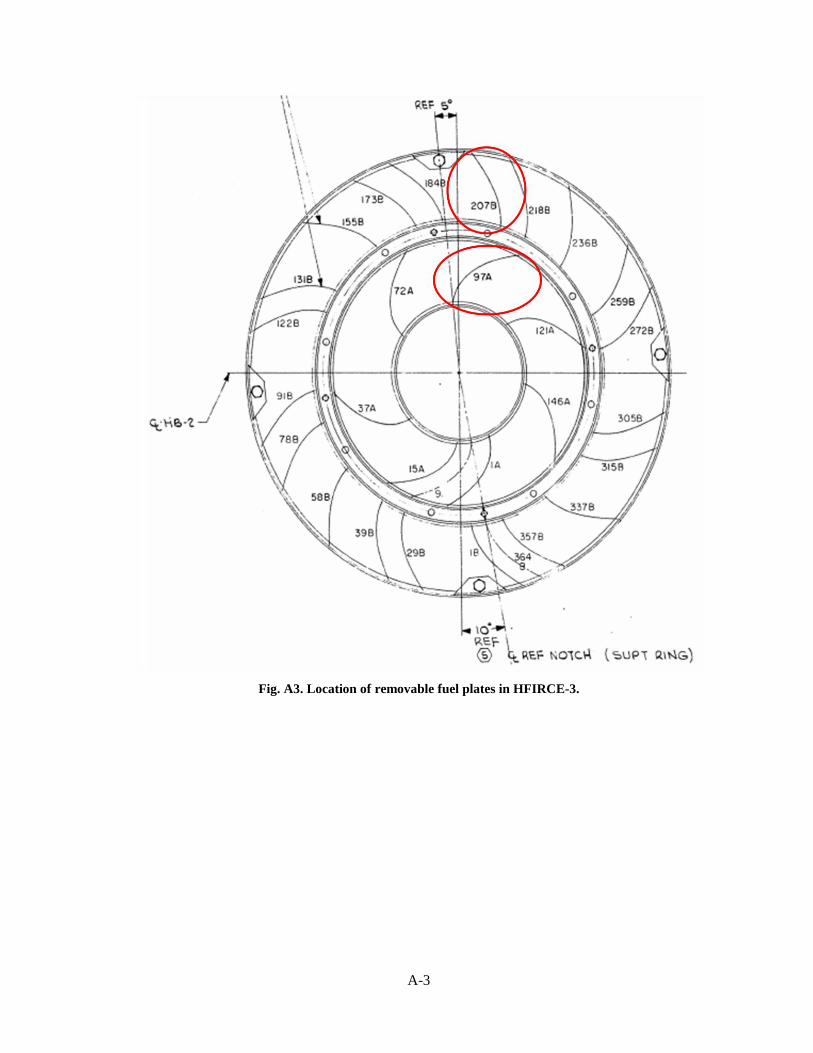
A-3

Fig. A3. Location of removable fuel plates in HFIRCE-3.

A-4

Table A1 lists the relative power densities corresponding to the clean core condition and

removable plates 97a and 207b in the IFE and OFE respectively, along with comparisons to other

measurements taken under the same clean core conditions, but on different days. Note the deviations

between the experiments. The data of September 8 had a negative bias because of a high-reading

normalizing foil and the data of October 21 showed a negative bias for foil positions 3, 4, 5, and 6 of

the OFE because of several acid rinses changing the clean core symmetrical rod positions.

Table A1. Comparison of power distribution data for the clean core condition and a (PI +W) target.

A-5

Table A2 lists the relative power densities corresponding to the fully poisoned core condition and

removable plates 97a and 207b in the IFE and OFE respectively, along with comparisons to another

measurement taken under fully poisoned core conditions, but on a different day. Note the deviations

between the experiments. The deviations between the two sets of data were caused by several

applications of boron and several acid rinses in between the two experiments and the elements being

inserted further on October 13.

Table A2. Comparison of power distribution data for the fully poisoned core condition and a (PI +W)

target.

A-6

This page blank.

A-7

ORNL/TM-2008/126

INTERNAL DISTRIBUTION

1. S. E. Burnette 10. R. W. Hobbs

2-4. D. Chandler 11. G. Ilas

5. R. A. Crone 12-14. R. T. Primm III

6. R. J. Ellis 15. K. A. Smith

7. M. B. Farrar 16. RRD-DCC-RC

8. J. C. Gehin 17. Laboratory Records-OSTI

9. G. J. Hertz

EXTERNAL DISTRIBUTION

18. R. D. Cheverton, 2703 West Gallaher Ferry Road, Knoxville, TN 37932.

19. Dr. H. D. Gougar, Manager, Fission and Fusion Systems, Idaho National Laboratory,

P.O. Box 1625, MS 3860, Idaho Falls, ID 83415-3860.

20. D. Kutikkad, Ph.D., Assistant Reactor Manager-Physics, University of Missouri Research

Reactor Facility, Columbia, MO 65211.

21. Dr. G. I. Maldonado, Associate Professor, University of Tennessee, Department of Nuclear

Engineering, 311 Pasqua Engineering Building, Knoxville, TN 37996-2300.

22. T. Newton, MIT Nuclear Reactor Laboratory, 138 Albany St., Cambridge, MA 02139.

23. R. D. Rothrock, 705 Cordova Lane, Lenoir City, TN 37771.

24. R. E. Williams, NIST Center for Neutron Research, 100 Bureau Drive, Stop 8560,

Gaithersburg, MD 20899.

25. Dr. John Christenson, Dept. of Mechanical Engineering, University of Cincinnati, Room 592,

Rhodes Hall, ML 72, P.O. Box 210072 Cincinnati, OH 45221-0072.

26. Dr. Henry Spitz, Dept. of Mechanical Engineering, University of Cincinnati, Room 592,

Rhodes Hall, ML 72, P.O. Box 210072 Cincinnati, OH 45221-0072.

27. A. Adams, U.S. Nuclear Regulatory Commission, One White Flint North, 11555 Rockville

Pike, Rockville, Maryland 20852-2738 ([email protected]).

38. G. S. Chang, Idaho National Laboratory, P.O. Box 1625, Idaho Falls, ID 83415-3885

([email protected]).

35. D. Diamond, Brookhaven National Laboratory, P.O. Box 5000, Upton, NY 11973-5000


41. J. Matos, Argonne National Laboratory, 9700 S. Cass Avenue, Argonne, IL 60439


mailto:[email protected]




validating mcnp for leu fuel design via power distribution

Documents