vad är entropi? - ifm...vad ar entropi?¨ i avsnitt 1.2 sysslade vi med system med m˚anga...
TRANSCRIPT

Vad är entropi?

2Exempel 4.1:Vi ar intresserade av ogonsumman; dvs summan av tarningarnas varden.Tva tarningar kan ge ogonsummorna 2, 3, 4, . . . , 12. Varje ogonsummautgor ett makrotillstand. Vilken ogonsumma far man oftast om mankastar tva tarningar? Att fa tva sexor sker inte ofta, det vet den somspelat tarningsspel. Visst hander det att man far tva sexor tva ganger irad. Men allteftersom man kastar fler ganger kommer ogonsumman 7oftast dyka upp. Varfor blir det sa? —Darfor att det ar mest sannolikt!Och varfor ar ogonsumman 7 mest sannolik? —Jo, darfor att man kan faogonsumman 7 pa flest olika satt!Ogonsumman 4 kan man fa pa flera olika satt, t ex om ena tarningenvisar 3 och den andra 1, eller genom att bada tarningarna visar 2. Ettannat satt ar kombinationen 3 och 1.
Tva tarningar kan bilda ogonsumman 4 pa tre olika satt, som visas ovan.Inom statistisk fysik skulle man kalla de tre tillstanden for mikrotillstand.De tre mikrotillstanden som visas svarar mot samma makrotillstand. Vihar alltsa ⌦ = 3 for makrotillstandet att ogonsumman ar 4.
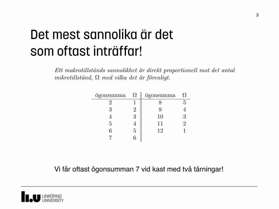
ogonsumma ⌦ ogonsumma ⌦2 1 8 53 2 9 44 3 10 35 4 11 26 5 12 17 6
Om man kastar tva tarningar sa far man oftast makrotillstandet attogonsumman ar 7 eftersom det ar forenligt med flest mikrotillstand!
4.2 Ordning och kaos
Betrakta en tepase. Vi vet fran vardagliga erfarenheter att om en tepaseplaceras i varmt vatten sa di↵underar temolekyler fran tepasen till resten avkoppen av varmt vatten. Pa samma satt om vi droppar nagra droppar black iett vattenbad, sa kommer blacket inte forbli koncentrerat till en droppe utanmoelkyulerna kommer att strava efter att blanda sig med vattnet och spridasig over hela vettenvolymen., jamnt fordelat. Vi kan forsoka tolka exempletmed tepasen utifran statistisk fysik.
Ögonsumman 4 kan skapas på 3 sätt:
Makrotillståndet ögonsumman 4.
3 mikrotillstånd är förenliga med makrotillståndet att ögonsumman är 4.
Mikrotillstånd och makrotillstånd
3
Exempel 4.1:Vi ar intresserade av ogonsumman; dvs summan av tarningarnas varden.Tva tarningar kan ge ogonsummorna 2, 3, 4, . . . , 12. Varje ogonsummautgor ett makrotillstand. Vilken ogonsumma far man oftast om mankastar tva tarningar? Att fa tva sexor sker inte ofta, det vet den somspelat tarningsspel. Visst hander det att man far tva sexor tva ganger irad. Men allteftersom man kastar fler ganger kommer ogonsumman 7oftast dyka upp. Varfor blir det sa? —Darfor att det ar mest sannolikt!Och varfor ar ogonsumman 7 mest sannolik? —Jo, darfor att man kan faogonsumman 7 pa flest olika satt!Ogonsumman 4 kan man fa pa flera olika satt, t ex om ena tarningenvisar 3 och den andra 1, eller genom att bada tarningarna visar 2. Ettannat satt ar kombinationen 3 och 1.
Tva tarningar kan bilda ogonsumman 4 pa tre olika satt, som visas ovan.Inom statistisk fysik skulle man kalla de tre tillstanden for mikrotillstand.De tre mikrotillstanden som visas svarar mot samma makrotillstand. Vihar alltsa ⌦ = 3 for makrotillstandet att ogonsumman ar 4.
ogonsumma ⌦ ogonsumma ⌦2 1 8 53 2 9 44 3 10 35 4 11 26 5 12 17 6
Om man kastar tva tarningar sa far man oftast makrotillstandet attogonsumman ar 7 eftersom det ar forenligt med flest mikrotillstand!
4.2 Ordning och kaos
Betrakta en tepase. Vi vet fran vardagliga erfarenheter att om en tepaseplaceras i varmt vatten sa di↵underar temolekyler fran tepasen till resten avkoppen av varmt vatten. Pa samma satt om vi droppar nagra droppar black iett vattenbad, sa kommer blacket inte forbli koncentrerat till en droppe utanmoelkyulerna kommer att strava efter att blanda sig med vattnet och spridasig over hela vettenvolymen., jamnt fordelat. Vi kan forsoka tolka exempletmed tepasen utifran statistisk fysik.
DEL 4
Vad
¨
ar entropi?
I avsnitt 1.2 sysslade vi med system med manga partiklar. Vi sag att vi kundesaga en hel del om systemet som helhet, utan att veta nagot om de enskildapartiklarnas rorelser. Man kan aven undersoka hur ett stort antal partiklar betersig sig statistiskt. Utgangspunkten ar att det mest sannolika ar det som troligenintra↵ar!
4.1 Mikro- och makrotillstand
Vi forestaller oss att vi har att gora med ett system som bestar av ett mycketstort antal identiska partiklar. Systemets tillstand kan beskrivas av storhetersasom energi, tryck, volym, eller temperatur. Ett visst varde pa en sadan storhetkallar vi makrotillstand. Makrotillstandet beskriver systemet som helhet, utanatt vi haller ordning pa varenda ingaende partikels lage och hastighet.
Den exakta konfigurationen for systemet kallas mikrotillstand, och ar enfullstandig beskrivning av varje ingaende partikels tillstand. Till varjemakrotillstand hor alltsa ett visst antal mikrotillstand.
Ett makrotillstands sannolikhet ar direkt proportionell mot det antalmikrotillstand, ⌦ med vilka det ar forenligt.
Det mest sannolika ar alltsa det som oftast sker.
39
Vi får oftast ögonsumman 7 vid kast med två tärningar!
Det mest sannolika är det som oftast inträffar!

4
Entropi
Logaritmen av antalet förenliga mikrotillstånd!
Magnetism
6
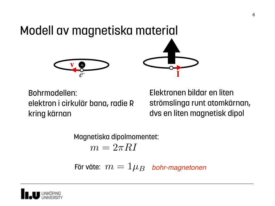
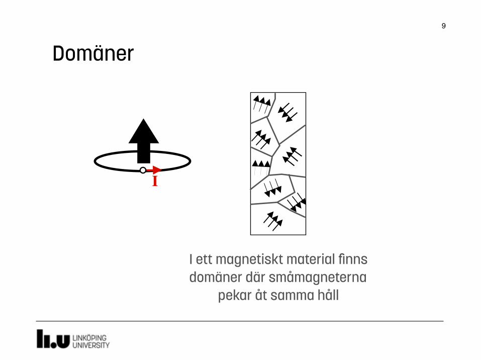
Elektronen bildar en liten strömslinga runt atomkärnan, dvs en liten magnetisk dipol
Modell av magnetiska material
DEL 5
Magnetism
Atomens magnetiska moment
5.1 Ferromagneter
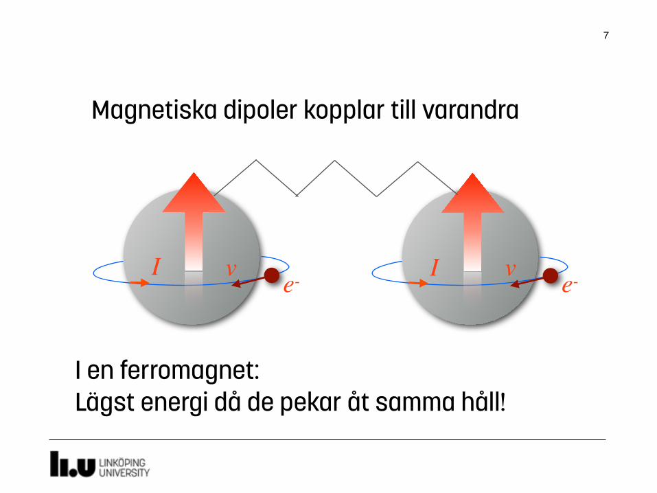
Ferromagnetism innebar att ett material uppvisar en spontan magnetisering,aven utan ett yttre palagt falt. Men vad orsakar ferromagnetism? Detta ar enbra fraga som egentligen inte kan fa nagot svar utan kvantmekanik ochrelativitetsteori. Man kan se varje atom som en liten stromslinga. Detta ger ettmagnetfalt, en magnetisk dipol, med en nord- och en sydande.
I en ferromagnet kan vi tanka oss att alla dipolerna ligger at samma hall,vilket ger ett starkt magnetfalt runt magneten. Nar vi hojer temperaturenupptacker vi nagot intressant. Vid en viss temperatur upphor magnetens falt!Detta kallas Curietemperaturen.
For att studera detta kan vi anvanda oss av en beromd modell: isingmodellen.
e-
e-+v
I
Friday, December 25, 2015
(a)
e-
e-+v
I
Friday, December 25, 2015
(b)
Figur 5.1
43
Bohrmodellen: elektron i cirkulär bana, radie R kring kärnan
m = 2⇡RI
För väte: m = 1µB
Magnetiska dipolmomentet:
bohr-magnetonen
7
Magnetiska dipoler kopplar till varandra
Ie-v I e-v
I en ferromagnet: Lägst energi då de pekar åt samma håll!

8
3.6 Finite temperature magnetism 25
(a) Ferromagnetic (b) 1Q antiferromagnetic
(c) 2Q antiferromagnetic (d) 3Q antiferromagneic
Figure 3.4. Di�erent ordered magnetic states shown on the fcc-lattice. (a) and (b)show ferromagnetic and 1Q anti-ferromagnetic arrangements, which are collinear. In thenon-collinear 2Q configuration (c), magnetic moments in alternating planes point towarda common center within the plane. In 3Q (d) all four moments in the magnetic unit cellpoint toward a common center.
Ferromagnet
9
I ett magnetiskt material finns domäner där småmagneterna
pekar åt samma håll
DEL 5
Magnetism
Atomens magnetiska moment
5.1 Ferromagneter
Ferromagnetism innebar att ett material uppvisar en spontan magnetisering,aven utan ett yttre palagt falt. Men vad orsakar ferromagnetism? Detta ar enbra fraga som egentligen inte kan fa nagot svar utan kvantmekanik ochrelativitetsteori. Man kan se varje atom som en liten stromslinga. Detta ger ettmagnetfalt, en magnetisk dipol, med en nord- och en sydande.
I en ferromagnet kan vi tanka oss att alla dipolerna ligger at samma hall,vilket ger ett starkt magnetfalt runt magneten. Nar vi hojer temperaturenupptacker vi nagot intressant. Vid en viss temperatur upphor magnetens falt!Detta kallas Curietemperaturen.
For att studera detta kan vi anvanda oss av en beromd modell: isingmodellen.
e-
e-+v
I
Friday, December 25, 2015
(a)
e-
e-+v
I
Friday, December 25, 2015
(b)
Figur 5.1
43
Domäner
10
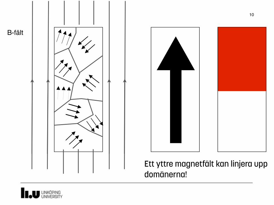
Externt magnetfält
Ett yttre magnetfält kan linjera upp domänerna!
B-fält
11
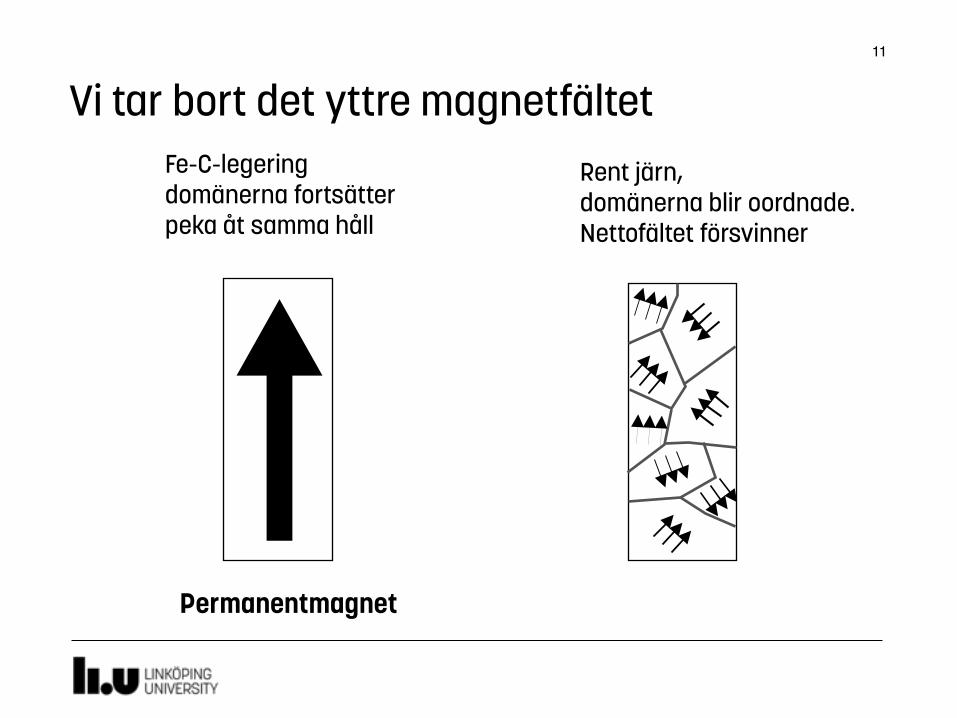
Fe-C-legering domänerna fortsätter peka åt samma håll
Rent järn, domänerna blir oordnade. Nettofältet försvinner
Vi tar bort det yttre magnetfältet
Permanentmagnet

12
=N
S
=N
S
En magnet har alltid två poler

13
3.6 Finite temperature magnetism 25
(a) Ferromagnetic (b) 1Q antiferromagnetic
(c) 2Q antiferromagnetic (d) 3Q antiferromagneic
Figure 3.4. Di�erent ordered magnetic states shown on the fcc-lattice. (a) and (b)show ferromagnetic and 1Q anti-ferromagnetic arrangements, which are collinear. In thenon-collinear 2Q configuration (c), magnetic moments in alternating planes point towarda common center within the plane. In 3Q (d) all four moments in the magnetic unit cellpoint toward a common center.

Ferromagnetism vid hög temperaturStatistisk mekanik

15
Curie-temperatur
Magnetiska egenskaperna uppträder under Curie-temperaturen

16
Magnetisering som funktion av temperatur
Curie-temperaturen
Ni
17
3.6 Finite temperature magnetism 27
(a)
(b)
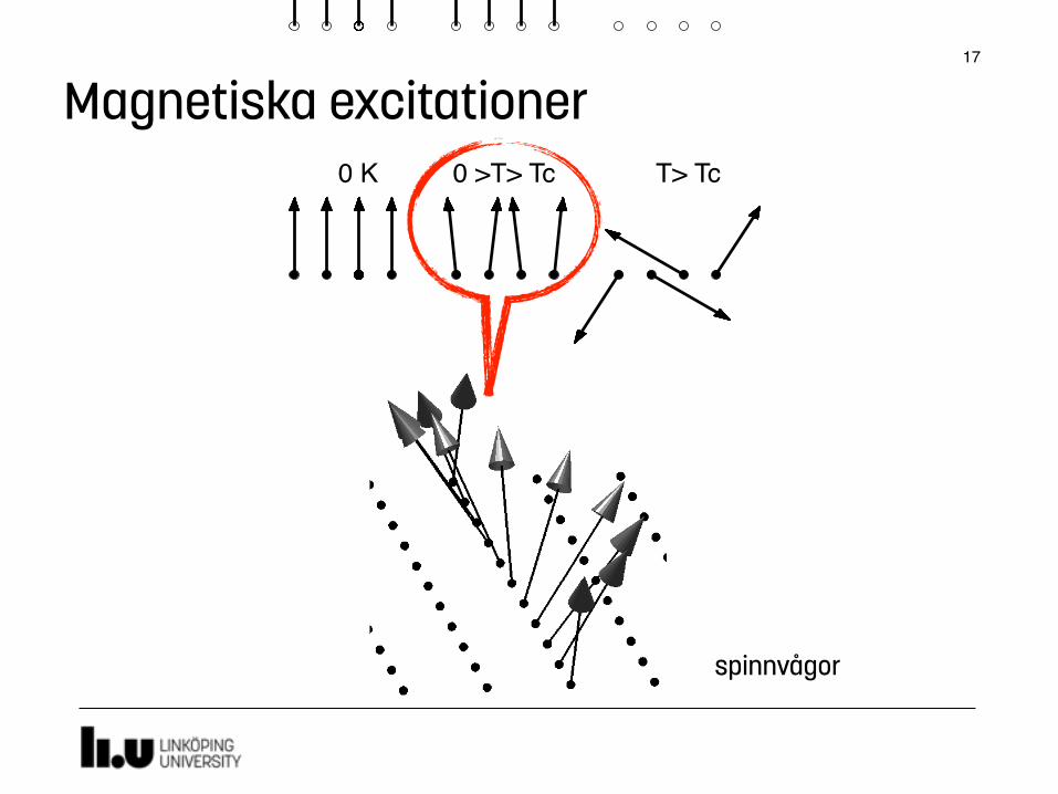
Figure 3.6. Two models of magnetic excitations in ferromagnets at finite temperature T ,relative to the Curie temperature, TC, in terms of local moments at the lattice sites. Leftpart shows the ferromagnetic ground state state at T = 0, middle part shows excitationsoccuring at 0 < T < TC, and the right part shows the paramagnetic state at T > TC.
debated in theory. Two mutually opposed pictures have emerged: the Stoner andthe Heisenberg pictures, which are illustrated in Figure 3.6, and will be furtherdiscussed in Sections 3.6.1 and 3.6.2.
3.6.1 Excitations in the ordered regime
Although the appearance of ferromagnetism in the ground states of Fe, Co andNi is correctly predicted by Stoner’s theory at T = 0 K, its extension to T > 0 Kfails badly, predicting extremely high Curie temperatures [40]. In this regime,these systems show many characteristics associated with the Heisenberg modelof localised magnetic moments. The fractional change of magnetisation at lowtemperature, with respect to the 0 K value, M0, has been verified experimentallyto obey:
M(T ) = M0
⇤1�
�T
TC
⇥3/2⌅
(3.13)
called the Bloch T 3/2 law [41]. Stoner theory fails to reproduce the Bloch law ofEquation (3.13), which has been confirmed for these materials.
0 K T> Tc 0 >T> Tc
Magnetiska excitationer
spinnvågor
IsingmodellenFerromagnetism vid hög temperatur

19
5.2 Isingmodellen
I Isingmodellen tanker vi oss att varje dipol endast kan anta vardena upp ellerned. Den totala magnetiseringen ar summan av dessa:
M =X
i
m
i
(5.1)
Da temperaturen hojs kan dipolerna flippa.FeNi modelled as 3-component alloy:
E0 = E[n0]
n(r) =X
i
��i
�i
�1
2�2 + Ve↵(r)
��
i
= �i
�i
Ve↵(r) = Vext(r) +
Zn(r�)
|r � r�|dr� + Vxc(r)
E[n] = Ts +
Zn(r)Vext(r)dr +
1
2
Z Zn(r)n(r�)
|r � r�| drdr� + Exc
e�
Vxc(r) =�Exc[n]
�n(r)
Ts
=X
i
h�i
| � 1
2�2|�
i
i
Fe1�c
Nic
! Fe1�c
Nic
FeNi ! Fe�(1+m)/2 Fe�
(1�m)/2 Ni
FeNi ! Fe�1�y
Fe�y
Nim = 1 � 2y We adopt a simple model.
Hconf =1
2
X
p
V (2)p
X
i,j�p
�ci
�cj
+1
3
X
q
V (3)q
X
i,j,k�q
�ci
�cj
�ck
+1
4
X
r
V (4)r
X
i,j,k,l�r
�ci
�cj
�ck
�cl
+ . . .
Hconf =1
2
X
p
V (2)p
X
i,j�p
�ci
�cj
+1
3
X
q
V (3)q
X
i,j,k�q
�ci
�cj
�ck
+1
4
X
r
V (4)r
X
i,j,k,l�r
�ci
�cj
�ck
�cl
+ . . .
1
78 Model Hamiltonians for finite temperature simulations
(a) Non-collinear disordered system. (b) Collinear disordered system.
Figure 8.2. Illustration of the principle behind the DLM model. A completely dis-ordered system of non-collinear magnetic moments can be modelled by a completelydisordered collinear system.
8.2.1 Disordered Local Moments
As discussed in the previous section, in a Heisenberg system, the local magneticmoments are insensitive to the local environment. It can be shown that a com-pletely disordered system of non-collinear local magnetic moments, can be mod-elled by a collinear state of disordered up and down local moments [170], as shownin Figure 8.2. This is called the disordered local moment model (DLM) [170],which provides a good representation of the Heisenberg picture of the paramag-netic state, shown in Figure 3.6(b). A magnetic atom, A, is then substituted by adisordered mixture of spin up and spin down atoms:
A ! A
"0.5A
#0.5 (8.11)
This fictitious alloy is e�ciently modelled with the CPA medium.However, not many systems can be considered Heisenberg systems, and this
approximation has its limitations. Ni is more di�cult than Fe in ab initio cal-culations because the exchange-interactions are more sensitive to the local envi-ronment. The experimentally verified paramagnetic state of Ni actually collapsesin DLM, but has been shown to be stabilised by inclusion of longitudinal spinfluctuations [169].
8.3 Cluster expansion of configurational energy
In order for the total energy of the system to be calculated e�ciently in eachMonte-Carlo cycle it is convenient to expand the configurational part of the total
G�1 = G�1KS � �
Gloc = P (C)GP (C)
Gimp
Gimp = Gloc
C
�� ⇡ �imp � �DC
�� � �imp � �DC
� = P (C)��P (C)
y (1)
y = 1y = 0.25y = 0.5
2
G�1 = G�1KS � �
Gloc = P (C)GP (C)
Gimp
Gimp = Gloc
C
�� ⇡ �imp � �DC
�� � �imp � �DC
� = P (C)��P (C)
y (1)
y = 1y = 0.25y = 0.5
2
G�1 = G�1KS � �
Gloc = P (C)GP (C)
Gimp
Gimp = Gloc
C
�� ⇡ �imp � �DC
�� � �imp � �DC
� = P (C)��P (C)
y (1)
y = 0y = 0.25y = 0.5
2
Paramagnetic state of a Heisenberg system
78 Model Hamiltonians for finite temperature simulations
(a) Non-collinear disordered system. (b) Collinear disordered system.
Figure 8.2. Illustration of the principle behind the DLM model. A completely dis-ordered system of non-collinear magnetic moments can be modelled by a completelydisordered collinear system.
8.2.1 Disordered Local Moments
As discussed in the previous section, in a Heisenberg system, the local magneticmoments are insensitive to the local environment. It can be shown that a com-pletely disordered system of non-collinear local magnetic moments, can be mod-elled by a collinear state of disordered up and down local moments [170], as shownin Figure 8.2. This is called the disordered local moment model (DLM) [170],which provides a good representation of the Heisenberg picture of the paramag-netic state, shown in Figure 3.6(b). A magnetic atom, A, is then substituted by adisordered mixture of spin up and spin down atoms:
A ! A
"0.5A
#0.5 (8.11)
This fictitious alloy is e�ciently modelled with the CPA medium.However, not many systems can be considered Heisenberg systems, and this
approximation has its limitations. Ni is more di�cult than Fe in ab initio cal-culations because the exchange-interactions are more sensitive to the local envi-ronment. The experimentally verified paramagnetic state of Ni actually collapsesin DLM, but has been shown to be stabilised by inclusion of longitudinal spinfluctuations [169].
8.3 Cluster expansion of configurational energy
In order for the total energy of the system to be calculated e�ciently in eachMonte-Carlo cycle it is convenient to expand the configurational part of the total
Disordered local moments (DLM)
Magnetic excitations
Wednesday, June 25, 2014
(a) Ferromagnet vid T = 0 K.
FeNi modelled as 3-component alloy:
E0 = E[n0]
n(r) =X
i
��i
�i
�1
2�2 + Ve↵(r)
��
i
= �i
�i
Ve↵(r) = Vext(r) +
Zn(r�)
|r � r�|dr� + Vxc(r)
E[n] = Ts +
Zn(r)Vext(r)dr +
1
2
Z Zn(r)n(r�)
|r � r�| drdr� + Exc
e�
Vxc(r) =�Exc[n]
�n(r)
Ts
=X
i
h�i
| � 1
2�2|�
i
i
Fe1�c
Nic
! Fe1�c
Nic
FeNi ! Fe�(1+m)/2 Fe�
(1�m)/2 Ni
FeNi ! Fe�1�y
Fe�y
Nim = 1 � 2y We adopt a simple model.
Hconf =1
2
X
p
V (2)p
X
i,j�p
�ci
�cj
+1
3
X
q
V (3)q
X
i,j,k�q
�ci
�cj
�ck
+1
4
X
r
V (4)r
X
i,j,k,l�r
�ci
�cj
�ck
�cl
+ . . .
Hconf =1
2
X
p
V (2)p
X
i,j�p
�ci
�cj
+1
3
X
q
V (3)q
X
i,j,k�q
�ci
�cj
�ck
+1
4
X
r
V (4)r
X
i,j,k,l�r
�ci
�cj
�ck
�cl
+ . . .
1
78 Model Hamiltonians for finite temperature simulations
(a) Non-collinear disordered system. (b) Collinear disordered system.
Figure 8.2. Illustration of the principle behind the DLM model. A completely dis-ordered system of non-collinear magnetic moments can be modelled by a completelydisordered collinear system.
8.2.1 Disordered Local Moments
As discussed in the previous section, in a Heisenberg system, the local magneticmoments are insensitive to the local environment. It can be shown that a com-pletely disordered system of non-collinear local magnetic moments, can be mod-elled by a collinear state of disordered up and down local moments [170], as shownin Figure 8.2. This is called the disordered local moment model (DLM) [170],which provides a good representation of the Heisenberg picture of the paramag-netic state, shown in Figure 3.6(b). A magnetic atom, A, is then substituted by adisordered mixture of spin up and spin down atoms:
A ! A
"0.5A
#0.5 (8.11)
This fictitious alloy is e�ciently modelled with the CPA medium.However, not many systems can be considered Heisenberg systems, and this
approximation has its limitations. Ni is more di�cult than Fe in ab initio cal-culations because the exchange-interactions are more sensitive to the local envi-ronment. The experimentally verified paramagnetic state of Ni actually collapsesin DLM, but has been shown to be stabilised by inclusion of longitudinal spinfluctuations [169].
8.3 Cluster expansion of configurational energy
In order for the total energy of the system to be calculated e�ciently in eachMonte-Carlo cycle it is convenient to expand the configurational part of the total
G�1 = G�1KS � �
Gloc = P (C)GP (C)
Gimp
Gimp = Gloc
C
�� ⇡ �imp � �DC
�� � �imp � �DC
� = P (C)��P (C)
y (1)
y = 1y = 0.25y = 0.5
2
G�1 = G�1KS � �
Gloc = P (C)GP (C)
Gimp
Gimp = Gloc
C
�� ⇡ �imp � �DC
�� � �imp � �DC
� = P (C)��P (C)
y (1)
y = 1y = 0.25y = 0.5
2
G�1 = G�1KS � �
Gloc = P (C)GP (C)
Gimp
Gimp = Gloc
C
�� ⇡ �imp � �DC
�� � �imp � �DC
� = P (C)��P (C)
y (1)
y = 0y = 0.25y = 0.5
2
Paramagnetic state of a Heisenberg system
78 Model Hamiltonians for finite temperature simulations
(a) Non-collinear disordered system. (b) Collinear disordered system.
Figure 8.2. Illustration of the principle behind the DLM model. A completely dis-ordered system of non-collinear magnetic moments can be modelled by a completelydisordered collinear system.
8.2.1 Disordered Local Moments
As discussed in the previous section, in a Heisenberg system, the local magneticmoments are insensitive to the local environment. It can be shown that a com-pletely disordered system of non-collinear local magnetic moments, can be mod-elled by a collinear state of disordered up and down local moments [170], as shownin Figure 8.2. This is called the disordered local moment model (DLM) [170],which provides a good representation of the Heisenberg picture of the paramag-netic state, shown in Figure 3.6(b). A magnetic atom, A, is then substituted by adisordered mixture of spin up and spin down atoms:
A ! A
"0.5A
#0.5 (8.11)
This fictitious alloy is e�ciently modelled with the CPA medium.However, not many systems can be considered Heisenberg systems, and this
approximation has its limitations. Ni is more di�cult than Fe in ab initio cal-culations because the exchange-interactions are more sensitive to the local envi-ronment. The experimentally verified paramagnetic state of Ni actually collapsesin DLM, but has been shown to be stabilised by inclusion of longitudinal spinfluctuations [169].
8.3 Cluster expansion of configurational energy
In order for the total energy of the system to be calculated e�ciently in eachMonte-Carlo cycle it is convenient to expand the configurational part of the total
78 Model Hamiltonians for finite temperature simulations
(a) Non-collinear disordered system. (b) Collinear disordered system.
Figure 8.2. Illustration of the principle behind the DLM model. A completely dis-ordered system of non-collinear magnetic moments can be modelled by a completelydisordered collinear system.
8.2.1 Disordered Local Moments
As discussed in the previous section, in a Heisenberg system, the local magneticmoments are insensitive to the local environment. It can be shown that a com-pletely disordered system of non-collinear local magnetic moments, can be mod-elled by a collinear state of disordered up and down local moments [170], as shownin Figure 8.2. This is called the disordered local moment model (DLM) [170],which provides a good representation of the Heisenberg picture of the paramag-netic state, shown in Figure 3.6(b). A magnetic atom, A, is then substituted by adisordered mixture of spin up and spin down atoms:
A ! A
"0.5A
#0.5 (8.11)
This fictitious alloy is e�ciently modelled with the CPA medium.However, not many systems can be considered Heisenberg systems, and this
approximation has its limitations. Ni is more di�cult than Fe in ab initio cal-culations because the exchange-interactions are more sensitive to the local envi-ronment. The experimentally verified paramagnetic state of Ni actually collapsesin DLM, but has been shown to be stabilised by inclusion of longitudinal spinfluctuations [169].
8.3 Cluster expansion of configurational energy
In order for the total energy of the system to be calculated e�ciently in eachMonte-Carlo cycle it is convenient to expand the configurational part of the total
Disordered local moments (DLM)
Magnetic excitations
Wednesday, June 25, 2014
(b) Temperaturen ar underCurietemperaturen: 0 < T < TC .FeNi modelled as 3-component alloy:
E0 = E[n0]
n(r) =X
i
��i
�i
�1
2�2 + Ve↵(r)
��
i
= �i
�i
Ve↵(r) = Vext(r) +
Zn(r�)
|r � r�|dr� + Vxc(r)
E[n] = Ts +
Zn(r)Vext(r)dr +
1
2
Z Zn(r)n(r�)
|r � r�| drdr� + Exc
e�
Vxc(r) =�Exc[n]
�n(r)
Ts
=X
i
h�i
| � 1
2�2|�
i
i
Fe1�c
Nic
! Fe1�c
Nic
FeNi ! Fe�(1+m)/2 Fe�
(1�m)/2 Ni
FeNi ! Fe�1�y
Fe�y
Nim = 1 � 2y We adopt a simple model.
Hconf =1
2
X
p
V (2)p
X
i,j�p
�ci
�cj
+1
3
X
q
V (3)q
X
i,j,k�q
�ci
�cj
�ck
+1
4
X
r
V (4)r
X
i,j,k,l�r
�ci
�cj
�ck
�cl
+ . . .
Hconf =1
2
X
p
V (2)p
X
i,j�p
�ci
�cj
+1
3
X
q
V (3)q
X
i,j,k�q
�ci
�cj
�ck
+1
4
X
r
V (4)r
X
i,j,k,l�r
�ci
�cj
�ck
�cl
+ . . .
1
78 Model Hamiltonians for finite temperature simulations
(a) Non-collinear disordered system. (b) Collinear disordered system.
Figure 8.2. Illustration of the principle behind the DLM model. A completely dis-ordered system of non-collinear magnetic moments can be modelled by a completelydisordered collinear system.
8.2.1 Disordered Local Moments
As discussed in the previous section, in a Heisenberg system, the local magneticmoments are insensitive to the local environment. It can be shown that a com-pletely disordered system of non-collinear local magnetic moments, can be mod-elled by a collinear state of disordered up and down local moments [170], as shownin Figure 8.2. This is called the disordered local moment model (DLM) [170],which provides a good representation of the Heisenberg picture of the paramag-netic state, shown in Figure 3.6(b). A magnetic atom, A, is then substituted by adisordered mixture of spin up and spin down atoms:
A ! A
"0.5A
#0.5 (8.11)
This fictitious alloy is e�ciently modelled with the CPA medium.However, not many systems can be considered Heisenberg systems, and this
approximation has its limitations. Ni is more di�cult than Fe in ab initio cal-culations because the exchange-interactions are more sensitive to the local envi-ronment. The experimentally verified paramagnetic state of Ni actually collapsesin DLM, but has been shown to be stabilised by inclusion of longitudinal spinfluctuations [169].
8.3 Cluster expansion of configurational energy
In order for the total energy of the system to be calculated e�ciently in eachMonte-Carlo cycle it is convenient to expand the configurational part of the total
G�1 = G�1KS � �
Gloc = P (C)GP (C)
Gimp
Gimp = Gloc
C
�� ⇡ �imp � �DC
�� � �imp � �DC
� = P (C)��P (C)
y (1)
y = 1y = 0.25y = 0.5
2
G�1 = G�1KS � �
Gloc = P (C)GP (C)
Gimp
Gimp = Gloc
C
�� ⇡ �imp � �DC
�� � �imp � �DC
� = P (C)��P (C)
y (1)
y = 1y = 0.25y = 0.5
2
G�1 = G�1KS � �
Gloc = P (C)GP (C)
Gimp
Gimp = Gloc
C
�� ⇡ �imp � �DC
�� � �imp � �DC
� = P (C)��P (C)
y (1)
y = 0y = 0.25y = 0.5
2
Paramagnetic state of a Heisenberg system
78 Model Hamiltonians for finite temperature simulations
(a) Non-collinear disordered system. (b) Collinear disordered system.
Figure 8.2. Illustration of the principle behind the DLM model. A completely dis-ordered system of non-collinear magnetic moments can be modelled by a completelydisordered collinear system.
8.2.1 Disordered Local Moments
As discussed in the previous section, in a Heisenberg system, the local magneticmoments are insensitive to the local environment. It can be shown that a com-pletely disordered system of non-collinear local magnetic moments, can be mod-elled by a collinear state of disordered up and down local moments [170], as shownin Figure 8.2. This is called the disordered local moment model (DLM) [170],which provides a good representation of the Heisenberg picture of the paramag-netic state, shown in Figure 3.6(b). A magnetic atom, A, is then substituted by adisordered mixture of spin up and spin down atoms:
A ! A
"0.5A
#0.5 (8.11)
This fictitious alloy is e�ciently modelled with the CPA medium.However, not many systems can be considered Heisenberg systems, and this
approximation has its limitations. Ni is more di�cult than Fe in ab initio cal-culations because the exchange-interactions are more sensitive to the local envi-ronment. The experimentally verified paramagnetic state of Ni actually collapsesin DLM, but has been shown to be stabilised by inclusion of longitudinal spinfluctuations [169].
8.3 Cluster expansion of configurational energy
In order for the total energy of the system to be calculated e�ciently in eachMonte-Carlo cycle it is convenient to expand the configurational part of the total
78 Model Hamiltonians for finite temperature simulations
(a) Non-collinear disordered system. (b) Collinear disordered system.
Figure 8.2. Illustration of the principle behind the DLM model. A completely dis-ordered system of non-collinear magnetic moments can be modelled by a completelydisordered collinear system.
8.2.1 Disordered Local Moments
As discussed in the previous section, in a Heisenberg system, the local magneticmoments are insensitive to the local environment. It can be shown that a com-pletely disordered system of non-collinear local magnetic moments, can be mod-elled by a collinear state of disordered up and down local moments [170], as shownin Figure 8.2. This is called the disordered local moment model (DLM) [170],which provides a good representation of the Heisenberg picture of the paramag-netic state, shown in Figure 3.6(b). A magnetic atom, A, is then substituted by adisordered mixture of spin up and spin down atoms:
A ! A
"0.5A
#0.5 (8.11)
This fictitious alloy is e�ciently modelled with the CPA medium.However, not many systems can be considered Heisenberg systems, and this
approximation has its limitations. Ni is more di�cult than Fe in ab initio cal-culations because the exchange-interactions are more sensitive to the local envi-ronment. The experimentally verified paramagnetic state of Ni actually collapsesin DLM, but has been shown to be stabilised by inclusion of longitudinal spinfluctuations [169].
8.3 Cluster expansion of configurational energy
In order for the total energy of the system to be calculated e�ciently in eachMonte-Carlo cycle it is convenient to expand the configurational part of the total
Disordered local moments (DLM)
Magnetic excitations
Wednesday, June 25, 2014
(c) Over Curietemperaturen T > TC ,totala magnetiseringen ar M = 0.
Figur 5.5: Isingmodellen av magnet da temperaturen hojs.
E
ij
= �Jm
i
· m
j
(5.2)
Vi betraktar en 1-dimensionell isingmodell av en ferromagnet, dar varjedipol vaxelverkar med sina narmsta grannar. Utbyteskonstanten ar alltsaJ > 0 mellan narmsta grannar och 0 annars. Konfigurationsenergi mellan tvapar ar alltsa: E = �Jm1m2. Antag att vi har periodiska randvillkor.
Exempel 5.1:
Isingmodellen Endast upp/ner
Kan göras på ett sätt=> entropin = 0
Kan göras på många sätt=> entropin maximal
ordning
oordning

20
TCurie
M=1
M=0
T=0 K
1-dimensionell ferromagnet, 10 magnetiska momentT
Två tävlande effekter i systemet• minimera interaktionsenergin => parallella moment• maximera entropin => oordnade moment
Temperaturen avgör vilken effekt som dominerar!
21
T1
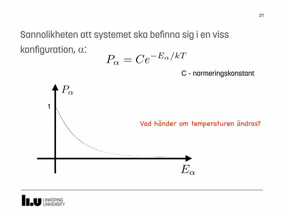
P↵ = Ce�E↵/kT
1
P↵ = Ce�E↵/kT
E↵
Sannolikheten att systemet ska befinna sig i en viss konfiguration, ⍺:
C - normeringskonstant
Vad händer om temperaturen ändras?

22
P⍺→β
T1
22
T2>T1
Eβ-E⍺
Sannolikheten för en ofördelaktig flipp är ökar med ökande T!
>0
P↵!� =e�E↵/kT
e�E�/kT= e�(E��E↵)/kT
Sannolikheten att systemet övergår till en konfiguration β där Eβ>E⍺

Monte Carlo-metodenSimulera magnetism

24
Kasinot i Monte Carlo, Monaco
Monte Carlo-metoder
25
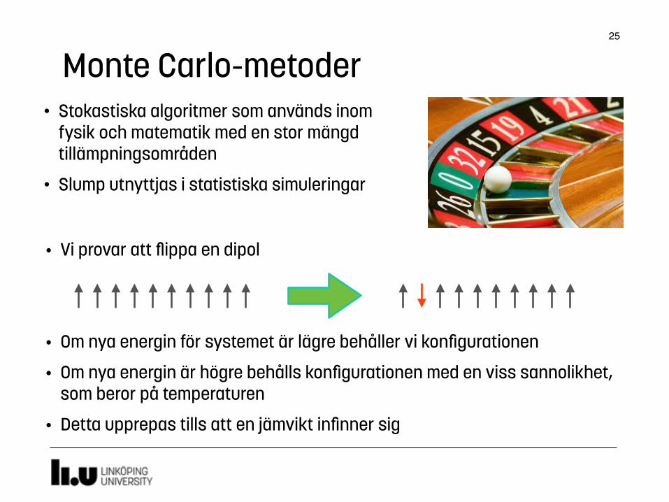
Monte Carlo-metoder• Stokastiska algoritmer som används inom
fysik och matematik med en stor mängd tillämpningsområden
• Slump utnyttjas i statistiska simuleringar
• Vi provar att flippa en dipol
• Om nya energin för systemet är lägre behåller vi konfigurationen
• Om nya energin är högre behålls konfigurationen med en viss sannolikhet, som beror på temperaturen
• Detta upprepas tills att en jämvikt infinner sig

flippa
välj en dipol
Eny < Egammal?Ja behåll
e-ΔE/kT? > slumptal
flippa tillbaka
Ja
Nej Nej
Monte Carlo-metoden