UvA-DARE is a service provided by the library of the University of Amsterdam (http://dare.uva.nl)

UvA-DARE (Digital Academic Repository)

Pulse dynamics in a three-component system: Existence analysis

Doelman, A.; van Heijster, P.; Kaper, T.J.

Published in:Journal of Dynamics and Differential Equations

DOI:10.1007/s10884-008-9125-2

Link to publication

Citation for published version (APA):Doelman, A., van Heijster, P., & Kaper, T. J. (2009). Pulse dynamics in a three-component system: Existenceanalysis. Journal of Dynamics and Differential Equations, 21(1), 73-115. https://doi.org/10.1007/s10884-008-9125-2

General rightsIt is not permitted to download or to forward/distribute the text or part of it without the consent of the author(s) and/or copyright holder(s),other than for strictly personal, individual use, unless the work is under an open content license (like Creative Commons).

Disclaimer/Complaints regulationsIf you believe that digital publication of certain material infringes any of your rights or (privacy) interests, please let the Library know, statingyour reasons. In case of a legitimate complaint, the Library will make the material inaccessible and/or remove it from the website. Please Askthe Library: https://uba.uva.nl/en/contact, or a letter to: Library of the University of Amsterdam, Secretariat, Singel 425, 1012 WP Amsterdam,The Netherlands. You will be contacted as soon as possible.

Download date: 19 Jun 2020

J Dyn Diff Equat (2009) 21:73–115DOI 10.1007/s10884-008-9125-2

Pulse Dynamics in a Three-Component System:Existence Analysis

Arjen Doelman · Peter van Heijster · Tasso J. Kaper

Received: 4 August 2007 / Revised: 5 June 2008 / Published online: 5 September 2008© The Author(s) 2008. This article is published with open access at Springerlink.com

Abstract In this article, we analyze the three-component reaction-diffusion system origi-nally developed by Schenk et al. (PRL 78:3781–3784, 1997). The system consists of bistableactivator-inhibitor equations with an additional inhibitor that diffuses more rapidly than thestandard inhibitor (or recovery variable). It has been used by several authors as a proto-type three-component system that generates rich pulse dynamics and interactions, and thisrichness is the main motivation for the analysis we present. We demonstrate the existenceof stationary one-pulse and two-pulse solutions, and travelling one-pulse solutions, on thereal line, and we determine the parameter regimes in which they exist. Also, for one-pulsesolutions, we analyze various bifurcations, including the saddle-node bifurcation in whichthey are created, as well as the bifurcation from a stationary to a travelling pulse, which weshow can be either subcritical or supercritical. For two-pulse solutions, we show that the thirdcomponent is essential, since the reduced bistable two-component system does not supportthem. We also analyze the saddle-node bifurcation in which two-pulse solutions are created.The analytical method used to construct all of these pulse solutions is geometric singularperturbation theory, which allows us to show that these solutions lie in the transverse inter-sections of invariant manifolds in the phase space of the associated six-dimensional travellingwave system. Finally, as we illustrate with numerical simulations, these solutions form the

A. Doelman · P. van HeijsterCentrum voor Wiskunde en Informatica (CWI), P.O. Box 94079, 1090 GB Amsterdam, The Netherlands

P. van Heijstere-mail: heijster@cwi.nl

A. DoelmanKorteweg-de Vries Instituut, Universiteit van Amsterdam, Plantage Muidergracht 24,1018 TV Amsterdam, The Netherlandse-mail: doelman@cwi.nl

T. J. Kaper (B)Department of Mathematics & Center for BioDynamics, Boston University, 111 Cummington Street,Boston, MA 02215, USAe-mail: tasso@math.bu.edu

123

74 J Dyn Diff Equat (2009) 21:73–115

backbone of the rich pulse dynamics this system exhibits, including pulse replication, pulseannihilation, breathing pulses, and pulse scattering, among others.

Keywords Three-component reaction-diffusion systems · One-pulse solutions · Travellingpulse solutions · Two-pulse solutions · Geometric singular perturbation theory ·Melnikov function

AMS (MOS) Subject Classifications Primary: 35K55 · 35B32 · 34C37 · Secondary:35K40

1 Introduction

Spatially localized structures, such as fronts, pulses and spots, have been found to exhibit awide variety of interesting dynamics in dissipative systems. These dynamics include repul-sion, annihilation, attraction, breathing, collision, scattering, self-replication, and spontane-ous generation. The richness of the observed dynamics typically increases with the complexityand the size of the system. Localized structures, that do not exist in reaction-diffusion (RD)systems with a small number of components, may readily exist when more components andmore terms are added to the system. Likewise, solutions that are unstable in small or simpleRD systems may become stable with such additions.

The aim of this article is to report on the mathematical analysis of a paradigm exam-ple that exhibits this increased richness. In particular, we study the three-component modelintroduced in [22] and studied further in [2,15,17,18,24,25]. In one space dimension, theequations are

⎧⎨

⎩

Ut = DU Uxx + f (U ) − κ3V − κ4W + κ1

τ Vt = DV Vxx + U − VθWt = DW Wxx + U − W.

(1.1)

where we used the notation of [15] and we note that (1.1) has the reversibility symmetryx → −x . Here, the (U, V )-subsystem is a classical, bistable two-component RD system,which exhibits dynamics similar to the classical FitzHugh–Nagumo equations (although hereDV �= 0, whereas DV = 0 in FHN), and the variable W denotes an added inhibitor compo-nent. We will show that it is responsible for increasing the richness of the types of solutionsthe model possesses.

In (1.1), U, V , and W are real-valued functions of x ∈ R and t ∈ R+, and the subscripts

indicate partial derivatives. The parameters τ and θ are positive constants, and the primaryinterest is in using τ as the bifurcation parameter. The diffusivities of the respective compo-nents are denoted by DU , DV , and DW , f (U ) is a bistable cubic reaction function (oftentaken to be f (U ) = 2U − U 3), κ3 and κ4 denote reaction rates, and κ1 denotes a constantsource term.

The fundamental discovery reported in [22] is that, in this three-component model, theadded component W can stabilize stationary and travelling single spot solutions and multi-spot solutions in two space dimensions, which otherwise are inherently unstable in the classi-cal two-component (U, V )-bistable model. This stabilization was shown to occur when DW

is sufficiently large relative to DU and DV , because then the presence of W prevents spotsfrom extending in the directions perpendicular to their directions of motion. In this manner,W suppresses the instability that spots undergo in two-component systems [22].

123

J Dyn Diff Equat (2009) 21:73–115 75

The dynamics of pulses in the one-dimensional model (1.1) is also known to be richer thanin the corresponding one-dimensional version of the two-component model. Pulses collide,scatter, annihilate, among others, as has been shown in [15,16], whereas the dynamics ofpulses in the restricted two-component system is much less rich. A special class of unsta-ble two-pulse solutions, called scattors or separators, is identified for (1.1) in [15,16]. It isshown that their stable and unstable manifolds organize the evolution in phase space of allnearby solutions. More precisely, during the course of a collision between two pulses, theyconverge to a separator state, and the location of the initial data relative to the stable andunstable manifolds of this separator determines how and when the pulses scatter off eachother. Furthermore, in some parameter regimes, the scattering process may be directed bya combination of two separators, where the colliding pulses first approach one separator,spend a long time near it, and then approach a second separator state, and then finally repelor annihilate, see [15,16].

Our work is inspired by the results from [18,22] and [15,16]. We carry out a complemen-tary, rigorous analysis of the existence of certain pulse solutions for a scaled version of thethree-component model, see (1.6) below. The model has a rich geometric structure that willbe studied using geometric singular perturbation theory, and we note that the application ofthis theory is challenging due to the fact that the associated ordinary differential equationsare six-dimensional.

1.1 Statement of the Model Equations

In [2,15,17,18,22,24,25], the numerical values of the diffusivities of the three species dif-fer by several orders of magnitude. For example, in [15], the values are DU = 5 × 10−6,DV = 5 × 10−5, and DW = 10−2. Therefore, we are motivated to introduce a scaled spatialvariable

x = x√DV

. (1.2)

For computational convenience we also scale out the factor two in the nonlinearity f (U ) =2U − U 3. Therefore, we introduce

t = 2t, (U , V , W ) = 1

2

√2(U, V, W ), (τ , θ ) = 2(τ, θ),

(κ1, κ3, κ4) = 1

2

(1

2

√2κ1, κ3, κ4

)

. (1.3)

In terms of these scaled quantities, the system (1.1) is

⎧⎨

⎩

Ut = ε2Ux x + U − U 3 − κ3V − κ4W + κ1

τ Vt = Vx x + U − VθWt = D2Wx x + U − W ,

(1.4)

with the nondimensional diffusivities ε2 = DU /(2DV ) � 1 and D2 = DW /DV � 1.As to the parameters in the reaction terms, the numerical values that are used in [15] are

(κ1, κ3, κ4) = (−7, 1, 8.5), and very similar values are used in [22]. While these are O(1)

with respect to ε, it is helpful to first study the system with O(ε) values of these parameters;i.e., to introduce scaled parameters, as follows:

κ1 = −εγ, κ3 = εα, κ4 = εβ, (1.5)

123

76 J Dyn Diff Equat (2009) 21:73–115

where α, β, and γ are O(1) quantities and where we have taken κ1 to be negative, since it isnegative in all of the above cited articles.

The rationale for this choice of scalings (1.5) is threefold. First, this choice was madeto facilitate the mathematical analysis, since in this regime the terms in the U -equationcorresponding to the source and to the coupling from the inhibitor components are weak, yetnot too weak. In fact, the effects of the source and the coupling terms are too weak whenthey are of O(ε2) [6]. Second, it turns out that much of the rich pulse dynamics exhibitedby system (1.4) exists also when the parameters have O(ε) values, as we will show in thisarticle (see also [19]). Therefore, one might reasonably hope to understand the origins of thedynamics observed in [15] by beginning with the present analysis. Third, in the numericalsimulations of [22,15], which were done on bounded domains, the W variable stays near−0.8, approximately. Hence, in a very approximate (and rough) sense one might argue, asfollows, that there is an effective impact of the parameters in the U -equation of (1.4) that isof O(ε). Since κ3 = 0.5 and ε = 1

10

√5 ≈ 0.22, the effect of V in this equation can indeed

be considered to be O(ε). Moreover, by the scalings (1.3), κ4W − κ1 ≈ 0.07 for W = −0.8(and κ1,4 as in [15]), which is clearly also O(ε). Thus, it appears that the impact of the sourceand coupling terms are indeed small.

In light of the above scalings, the model equations that we study are⎧⎨

⎩

Ut = ε2Uxx + U − U 3 − ε(αV + βW + γ )

τ Vt = Vxx + U − VθWt = D2Wxx + U − W,

(1.6)

where we dropped the tildes. Furthermore, we require that 0 < ε � 1, 0 < τ, θ � 1/ε3,D > 1, and α, β, γ ∈ R, where the upper bound on τ and θ is derived in Sect. 3.1. Moreover,we assume that the solutions (U (x, t), V (x, t), W (x, t)) are bounded over the entire domain.

At various stages throughout the analysis, we will see that it is also useful to examine thethree-component model in a stretched (or ‘fast’) spatial variable ξ = x/ε:

⎧⎪⎨

⎪⎩

Ut = Uξξ + U − U 3 − ε(αV + βW + γ )

τ Vt = 1ε2 Vξξ + U − V

θWt = D2

ε2 Wξξ + U − W.

(1.7)

We refer to this system as the fast system, and to system (1.6) as the slow system.The system (1.6) or (1.7) is well-suited as a paradigm for the analysis of three-component

RD systems. On the one hand, it is sufficiently nonlinear and complex so that it supports arich variety of localized structures, and on the other hand it is sufficiently simple, with linearreaction functions in the second and third components and with linear coupling, so that muchof the dynamics can be computed analytically, including certain bifurcations. See also [23].In this respect, we believe that the results presented here also provide a basis to establish atheory of interacting pulses in this paradigm model.

1.2 Outline of the Main Results

We begin in Sect. 2 with examining the stationary, or standing, one-pulse solutions. Forthese solutions, the U -component consists of a front, which connects the (quiescent) stateU = −1 +O(ε) to the (active) state U = 1 +O(ε), and a back, which provides the oppositeconnection, concatenated together to form a pulse (or homoclinic orbit). Both the front andthe back are sharp, so that the pulse is highly localized, due to the asymptotically small valueof ε2 in (1.6). The V -component of the one-pulse solutions consists of a smooth pulse that

123

J Dyn Diff Equat (2009) 21:73–115 77

−1000 −500 0 500 1000−1.5

−1

−0.5

0

0.5

1

1.5

−1000 −500 0 500 1000−1.5

−1

−0.5

0

0.5

1

1.5

WV

UU

V

W

x x

Fig. 1 Stable stationary one-pulse and two-pulse solutions of system (1.6) obtained via numerical simula-tion. For the one-pulse the system parameters are (α, β, γ, D, τ, θ, ε) = (3, 1, 2, 5, 1, 1, 0.01), and for thetwo-pulse we had (α, β, γ, D, τ, θ, ε) = (2, −1, −0.25, 5, 1, 1, 0.01)

is centered on the middle of the interval in which the U -component is in the active stateand that varies over slightly wider interval than the U -pulse. Finally, the W -component alsoconsists of a single, smooth pulse, but it varies on a wider interval than either of the othertwo components due to the fact that D > 1. See Fig. 1. The standing one-pulse solutions areformally constructed in Sect. 2.2. Then, we make this construction rigorous in Theorem 2.1,which states that the three-component model (1.6) possesses standing one-pulse solutionswhenever the system parameters satisfy (2.22). See Sect. 2.3 for the statement of this theoremand Sect. 2.4 for its proof.

Next, we analyze the existence of travelling one-pulse solutions. This analysis, presentedin Sect. 3, follows the same two-step procedure: we first construct solutions formally (seeSect. 3.1) and then we prove their existence rigorously (see Sects. 3.2 and 3.3). The mainresult is Theorem 3.1, which states that there exist travelling pulse solutions whenever eitherτ or θ (or both) is O(1/ε2) and the system parameters satisfy (3.13).

Given these results about standing and travelling one-pulse solutions, it is of interest toinvestigate the bifurcation of the former into the latter. We do so in Sect. 4. The leadingorder results are given by (4.2) in Sect. 4.1, and then the rigorous, high-order asymptoticsfor the main bifurcation parameter τ as a function of the other parameters is summarizedin Lemma 4.1, see Sect. 4.2. It turns out that this bifurcation can be supercritical, as well assubcritical, depending on the parameters, see Corollaries 4.2 and 4.3. This result contrastswith the bifurcation result for the two-dimensional version of this model, obtained in [18],where it was shown that this bifurcation is supercritical.

Having completed our analysis of the one-pulse solutions, we next turn our attention totwo-pulse solutions of (1.6). The main result is Theorem 5.1, which guarantees the existenceof two-pulse solutions whenever the system parameters satisfy (5.6). These two-pulse solu-tions have U -components that consist of two copies of the U -component of the single pulses,while the V - and W -components exhibit two peaks as well, but are not near equilibrium inthe interval between their two peaks. See Fig. 1. In this sense, the interaction between thepulses is semi-strong, according to the terminology of [3]. We also note that (5.6) is rathercomplex, and we present investigations of it when D = 2, and when D is general. Moreover,we give the asymptotics of the key quantities as D → ∞. See Sects. 5.2 and 5.3, respectively.

123

78 J Dyn Diff Equat (2009) 21:73–115

After completing the analysis of these pulse solutions, we examine in Sect. 6 the two-com-ponent (U, V )-subsystem, obtained from (1.6) by setting W constant at −1. This analysis ofthe two-component system enables us to make observations about the differences between thetwo-component and the three-component systems. For instance, for the two-pulse solutions,we observe that the inclusion of the third component is essential, because the two-componentversion of the model cannot possess two-pulse solutions. Simply put, there is not enough free-dom in the two-component model to permit for the construction of these solutions, and ouranalysis reveals why the third component—which naturally makes the phase space of the asso-ciated ODE problem six-dimensional—creates sufficient space/freedom for their existence.

In Sect. 7.1 we present the results of a series of numerical simulations of (1.6). Thesesimulations confirm the various analytical existence and bifurcation results presented herein,and they also reveal the presence of rich pulse interactions, including pulse reflection andannihilation, stable breathing single and double pulses (which bifurcate from stationary pulsesolutions), pulse scattering, as well as combinations of these. See Figs. 14–18. The single anddouble pulses analyzed in this article are key building blocks to understand these rich pulseinteractions. Finally, in Sect. 7.2, we summarize our analysis and discuss some related items.

Remark 1.1 The two-pulse solutions constructed in [7,10] for the FHN system differ inseveral respects from those constructed here. In FHN, these are essentially copies of the one-pulse solution, that must be very far apart, and that exhibit oscillatory behavior in the intervalbetween the pulses. The mechanism responsible for their existence is related to the classicalShilnikov mechanism.

Remark 1.2 Other examples of stabilization via the inclusion of an additional componentin a model are given for instance by the Gray–Scott and Gierer–Meinhardt systems. In these,one-pulse (homoclinic) solutions that are unstable with respect to the scalar RD equation forthe activator component are stabilized in certain parameter regimes by the coupling to theequation for the inhibitory component. The diffusive flux of inhibitor into the pulse domainshelps to localize the activator concentration, hence stabilizing one-pulse solutions, and werefer to [3,5] for the mathematical analysis using the Evans function and the stability index.Moreover, it is is worth noting that the converse may also arise; namely in [6] it is shown thatstable fronts of a bistable, scalar RD equation are destabilized through coupling to a secondcomponent when the parameters are chosen so that either the essential spectrum approachesthe origin or an eigenvalue emerges from the essential spectrum and becomes unstable.

2 Stationary One-Pulse Solutions

2.1 Basic Observations

First, we look at stationary pulses of system (1.7), i.e., we put (Ut , Vt , Wt ) = (0, 0, 0). Byintroducing p = uξ , q = 1

εvξ and r = D

εwξ , we transform system (1.7) into a six-dimen-

sional singular perturbed ordinary differential equation (ODE)⎧⎪⎪⎪⎪⎪⎪⎨

⎪⎪⎪⎪⎪⎪⎩

uξ = ppξ = −u + u3 + ε(αv + βw + γ )

vξ = εqqξ = ε(v − u)

wξ = εD r

rξ = εD (w − u).

(2.1)

123

J Dyn Diff Equat (2009) 21:73–115 79

Although ξ is the spatial variable, it will play the role of ‘time’ in our analysis. The systempossesses two symmetries

ξ → −ξ, p → −p, q → −q, r → −r

u → −u, p → −p, v → −v, q → −q, w → −w, r → −r, γ → −γ. (2.2)

Note that the first symmetry corresponds to the reversibility symmetry (x, ξ) → (−x,−ξ)

in (1.6) and (1.7), respectively. The fixed points of system (2.1) have p = q = r = 0, andu = v = w with u3 + u(−1 + ε(α + β)) + εγ = 0. Solving this last equation yields

u±ε = ±1 ∓ 1

2ε (α + β ± γ ) + O(ε2), u0

ε = εγ + O(ε2). (2.3)

Hence, there are three fixed points,

P±ε = (u±

ε , 0, u±ε , 0, u±

ε , 0), P0ε = (u0

ε, 0, u0ε, 0, u0

ε, 0). (2.4)

It can be checked [23] that P±ε , respectively P0

ε , represent stable, respectively unstable, trivialstates of the PDE (1.6) and (1.7).

The fast reduced system (FRS) is obtained by letting ε ↓ 0 in (2.1),{

uξ = ppξ = −u + u3,

(2.5)

as well as (vξ , qξ , wξ , rξ ) = (0, 0, 0, 0), i.e., (v, q, w, r) ≡ (v∗, q∗, w∗, r∗) with v∗, q∗, w∗,r∗ ∈ R constants. The fixed points of the FRS are given by (u, p) ∈ {(±1, 0), (0, 0)}. Theformer are saddles. The latter, (0, 0), is a center that corresponds to P0

ε and thus to an unstabletrivial state of (1.6)—we will therefore not consider it.

We define the four-dimensional invariant manifolds M±0 by

M±0 := {(u, p, v, q, r, w) ∈ R

6 : u = ±1, p = 0},which are the unions of the saddle points over all possible v∗, q∗, w∗, r∗ ∈ R. Planar system(2.5) is integrable with Hamiltonian

H(u, p) = 1

2(p2 + u2) − 1

4(u4 + 1), (2.6)

which is chosen such that H(u, p) = 0 on M±0 . The FRS possesses heteroclinic orbits

(u0,±h (ξ), p0,±

h (ξ)) that connect the fixed points (u, p) = (±1, 0) to (u, p) = (∓1, 0),

u0,±h (ξ) = ∓ tanh

(1

2

√2ξ

)

, p0,±h (ξ) = ∓1

2

√2sech2

(1

2

√2ξ

)

. (2.7)

See Fig. 2. The manifolds M±0 are normally hyperbolic, and they have five-dimensional stable

and unstable manifolds W u,s(M±0 ) that are the unions of the four-parameter (v∗, q∗, w∗, r∗)-

families of one-dimensional stable and unstable manifolds of the saddle points (u, p) =(±1, 0) in (2.5).

Fenichel’s first persistence theorem [8,11,14] implies that for ε small enough, system(2.1) has locally invariant slow manifolds M±

ε which are O(ε) C1-close to M±0 , i.e., M±

ε

can be represented by

M±ε := {u = ±1 + εu±

1 (v, q, w, r; ε), p = εp±1 (v, q, w, r; ε)}, (2.8)

123

80 J Dyn Diff Equat (2009) 21:73–115

-2 -1 1 2

-2

-1

1

2

Fig. 2 The phase portrait of the fast reduced Hamiltonian system (2.5)

where the graphs u1 and p1 can be computed by an expansion in ε,

M±ε = {u = ±1 − 1

2ε (αv + βw + γ ) + O(ε2), p = O(ε2)}. (2.9)

The application of Fenichel’s second persistence theorem establishes that M±ε have five-

dimensional stable and unstable manifolds, W s,u(M±ε ), that are O(ε) C1-close to their ε = 0

counterparts W u,s(M±0 ). Observe that the critical points P±

ε have three-dimensional stableand unstable manifolds W u,s(P±

ε ) which are contained in W u,s(M±ε ).

There are two slow reduced limit systems (SRS), both of which we write in terms of thefast variable ξ : one that governs the flow on M−

ε ,{

vξξ = ε2(v + 1 + O(ε)),

wξξ = ε2

D2 (w + 1 + O(ε)),(2.10)

and one that governs the flow on M+ε ,

{vξξ = ε2(v − 1 + O(ε)),

wξξ = ε2

D2 (w − 1 + O(ε)).(2.11)

Observe that (v, q, w, r) = (±1, 0,±1, 0)+O(ε) are saddle points on M±ε that correspond

to the fixed points P±ε (2.4). Also note that the v- and w-equations are decoupled, so that

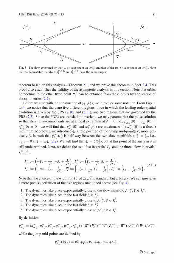
both ODEs can be considered separately. See also Remark 2.1. Hence, we have a (v, q)-subsystem and a (w, r)-subsystem, both with two saddle points. These four saddle pointseach have one-dimensional stable and unstable manifolds, lu,s,±

v,w , that are given to leadingorder by

u,±v = {q = ∓1 + v}, u,±

w = {r = ∓1 + w},s,±v = {q = ±1 − v}, s,±

w = {r = ±1 − w}. (2.12)

In Fig. 3, we sketch some orbits on the manifolds M±ε .

2.2 The Construction of One-Pulse Solutions γ −h, j (ξ) Homoclinic to P−

ε

In this section, we consider symmetric standing one-pulse solutions γ −h, j (ξ) that are homo-

clinic to P−ε . Here, we present the formal derivation. Then, in Sect. 2.3, we formulate a

123

J Dyn Diff Equat (2009) 21:73–115 81

Fig. 3 The flow generated by the (v, q)-subsystem on M−ε and that of the (w, r)-subsystem on M+

ε . Notethat stable/unstable manifolds lu,s,±

v and lu,s,∓w have the same slopes

theorem based on this analysis—Theorem 2.1, and we prove this theorem in Sect. 2.4. Thisproof also establishes the validity of the asymptotic analysis in this section. Note that orbitshomoclinic to the other fixed point P+

ε can be obtained from these orbits by application ofthe symmetries (2.2).

Before we start with the construction of γ −h, j (ξ), we introduce some notation. From Figs. 1

to 4, we notice that there are five different regions, three in which the leading order spatialevolution is given by the SRS (2.10) and (2.11), and two regions that are governed by theFRS (2.5). Since the PDEs are translation invariant, we may parametrize the pulse solutionso that its u, v, w-components are at a local extremum at ξ = 0, i.e., p−

h, j (0) = q−h, j (0) =

r−h, j (0) = 0—we will find that v−

h, j (0) and w−h, j (0) are maxima, while u−

h, j (0) is a (local)minimum. Moreover, we introduce ξ∗ as the position of the ‘jump mid-point(s)’, more pre-cisely ξ∗ is such that γ −

h, j (ξ) is half-way between the two slow manifolds at ξ = ξ∗, i.e.,

u−h, j = 0 at ξ = ±ξ∗ (2.2). We will find that ξ∗ = O( 1

ε), but at this point of the analysis it is

still undetermined. Next, we define the two ‘fast intervals’ I ∓f and the three ‘slow intervals’

I ∓s , I 0

s ,

I −f :=

(−ξ∗ − 1√

ε,−ξ∗ + 1√

ε

), I +

f :=(ξ∗ − 1√

ε, ξ∗ + 1√

ε

),

I −s :=

(−∞,−ξ∗ − 1√

ε

], I 0

s :=[−ξ∗ + 1√

ε, ξ∗ − 1√

ε

], I +

s :=[ξ∗ + 1√

ε,∞

).

(2.13)

Note that the choice of the width for I ±f of 2/

√ε is standard, but arbitrary. We can now give

a more precise definition of the five regions mentioned above (see Fig. 4).

1. The dynamics take place exponentially close to the slow manifold M−ε : ξ ∈ I −

s .2. The dynamics take place in the fast field: ξ ∈ I −

f .

3. The dynamics take place exponentially close to M+ε : ξ ∈ I 0

s .4. The dynamics take place in the fast field: ξ ∈ I +

f .5. The dynamics take place exponentially close to M−

ε : ξ ∈ I +s .

By definition,

γ −h, j = (u−

h, j , p−h, j , v

−h, j , q−

h, j , w−h, j , r−

h, j ) ∈ W u(P−ε ) ∩ W s(P−

ε ) ⊂ W u(M−ε ) ∩ W s(M−

ε ),

while the jump mid-points are defined by

γ −h, j (±ξ∗) = (0,∓p∗, v∗,∓q∗, w∗,∓r∗).

123

82 J Dyn Diff Equat (2009) 21:73–115

Fig. 4 A schematic sketch of a standing pulse solution γ −h, j (ξ) in the six-dimensional (u, p, v, q, w, r)—

phase space. In region 1, the pulse is exponentially close to M−ε for a long ‘spatial time’ and approaches P−

ε

as ξ → −∞. It ‘takes off’ from M−ε at ξ = −ξ∗ − 1√

ε(by definition) and ‘jumps’ through the fast field

(ξ ∈ I−f ) towards M+

ε —this is region 2. In region 3, γ −h, j (ξ) touches down near M+

ε at ξ = −ξ∗ + 1√ε

and remains exponentially close to M+ε until ξ = ξ∗ − 1√

ε, from where it jumps back towards M−

ε , which

defines region 4 (ξ ∈ I+f ). In the final region, 5, γ −

h, j (ξ) is again exponentially close to M−ε and approaches

P−ε as ξ → ∞. See also Fig. 1 in which γ −

h, j (ξ) exhibits the same structure

Furthermore, since γ −h, j (ξ) remains exponentially close to M+

ε for ξ ∈ I 0s , γh, j (ξ) is also

exponentially close to W u(P−ε )∩W s(M+

ε ) and to W s(P−ε )∩W u(M+

ε ) for sufficiently longtime. Note that γ −

h, j (ξ) /∈ W u(M−ε ) ∩ W s(M+

ε ) or W s(M−ε ) ∩ W u(M+

ε ), since it has to beable to jump back again from M+

ε to M−ε .

By considering possible take off and touch down points of jumps through the fast field andby studying, in fact explicitly solving, the slow flows on M−

ε (2.10) and on M+ε (2.11), we

obtain relations between the coordinates (v∗,∓q∗, w∗,∓r∗) of the jump mid-points and theirspatial positions ±ξ∗ that uniquely determine the homoclinic orbit(s) γ −

h, j (ξ); see Remark2.1.

For ε �= 0, the Hamiltonian H(u, p) (2.6) is not conserved

d

dξH(u(ξ), p(ξ)) = uuξ + ppξ − u3uξ

= up + p(−u + u3 + ε(αv + βw + γ )

)− u3 p (2.14)

= εp(αv + βw + γ ).

Since (u−h, j (ξ), p−

h, j (ξ)) must be O(ε) close to the heteroclinic solution (u0,−h (ξ), p0,−

h (ξ))

(2.7) of the FRS (2.5) in the fast field I −f , the total change in H for an orbit γ −

h, j (ξ) thatjumps from M−

ε to M+ε is approximated by

−f H(v∗, q∗, w∗, r∗) =

∫

I −f

Hξ dξ

=∫

I −f

εp0,−h (ξ + ξ∗)(αv∗ + βw∗ + γ )dξ + O(ε

√ε)

123

J Dyn Diff Equat (2009) 21:73–115 83

= ε(αv∗ + βw∗ + γ )

∞∫

−∞p0,−

h (ξ)dξ + O(ε√

ε)

= 2ε(αv∗ + βw∗ + γ ) + O(ε√

ε),

where we have used (2.7), (2.14), and assumed that ξ∗ = O( 1ε). Note that −

f H in principledepends on (v∗, q∗, w∗, r∗), the slow (v, q, w, r)-coordinates of the jump mid-points, andthat these coordinates do not vary to leading order during a jump through the fast field,

−f v = ∫

I −f

vξ dξ = ∫

I −f

εqdξ = 2q∗√

ε + O(ε) = O(√

ε),

−f q = ∫

I −f

qξ dξ = ∫

I −f

ε(v − u)dξ = 2v∗√

ε + O(ε) = O(√

ε),

−f w = ∫

I −f

wξ dξ = ∫

I −f

εD rdξ = 2r∗ 1

D

√ε + O(ε) = O(

√ε),

−f r = ∫

I −f

rξ dξ = ∫

I −f

εD (w − u)dξ = 2w∗ 1

D

√ε + O(ε) = O(

√ε).

(2.15)

On the other hand, such an orbit γ −h, j (ξ) cannot have a total change of more than O(ε2) over

a jump through the fast field I −f , since

H(u, p)|M±ε

= 1

2

((

±1 − 1

2ε(αv + βw + γ ) + O(ε2)

)2

+ O(ε2)2

)

−1

4

((

±1 − 1

2ε(αv + βw + γ ) + O(ε2)

)4

+ 1

)

= 1

2∓ 1

2ε(αv + βw + γ ) − 1

4± 1

2ε(αv + βw + γ ) − 1

4+ O(ε2) = O(ε2),

(2.16)

where we recall (2.8) and (2.9). Thus, we conclude that for an orbit γ −h, j (ξ) that jumps from

M−ε to M+

ε the following relation for the slow (v∗, q∗, w∗, r∗)-coordinates of the jumpmid-point must hold to leading order

αv∗ + βw∗ + γ = 0. (2.17)

Note that −f H(v∗, q∗, w∗, r∗) is in fact a Melnikov function that measures the distance

between W u(M−ε ) and W s(M+

ε ) as they intersect the {u = 0} hyperplane (see [3,6,20]).Condition (2.17) determines the three-dimensional set of initial conditions in {u = 0} thatdefines the four-dimensional intersection of the two five-dimensional manifolds W u(M−

ε )

and W s(M+ε ) (recall that the phase space is six-dimensional and that the p-coordinates of

these initial conditions are necessarily O(ε) close to p0,−h (0) = 1

2

√2 (2.7)).

By the reversibility symmetry (2.2), we know that (2.17) also must hold for the (v∗,−q∗,w∗,−r∗)-coordinates, which are the coordinates of the jump mid-points of the orbits thatjump from M+

ε to M−ε near ξ = ξ∗.

Next, we study the slow flows on M±ε . The Eqs. 2.10 and 2.11 for these flows are linear

and decoupled, thus we may solve for v and w separately. Based on the above analysis, wewrite down the following boundary conditions for the solutions in regions 1, 3, and 5:

123

84 J Dyn Diff Equat (2009) 21:73–115

vh(±∞) = −1, vh

(−ξ∗ ± 1√

ε

)= vh

(ξ∗ ∓ 1√

ε

)= v∗ + O(

√ε),

qh(±∞) = 0, qh

(−ξ∗ ± 1√

ε

)= −qh

(ξ∗ ∓ 1√

ε

)= q∗ + O(

√ε),

wh(±∞) = −1, wh

(−ξ∗ ± 1√

ε

)= wh

(ξ∗ ∓ 1√

ε

)= w∗ + O(

√ε),

rh(±∞) = 0, rh

(−ξ∗ ± 1√

ε

)= −rh

(ξ∗ ∓ 1√

ε

)= r∗ + O(

√ε),

(2.18)

see Figs. 1 and 4. Note that there are more (boundary) conditions than free parameters in thegeneral solutions of (2.10) and (2.11). As a consequence, we find that both v∗ and q∗, as wellas w∗ and r∗, must be related,

q∗ = v∗ + 1, r∗ = w∗ + 1, (2.19)

which in geometrical terms is equivalent to (v∗, q∗) ∈ u,−v , and (w∗, r∗) ∈ u,−

w (2.12), seealso Fig. 3. Moreover, (2.18) yields additional relations between v∗ and ξ∗ and between w∗and ξ∗,

v∗ = −A2, w∗ = −A2D where A = e−εξ∗ . (2.20)

Observe that, since ξ∗ > 0, A ∈ (0, 1), so that v∗, w∗ ∈ (−1, 0). For (v∗, q∗, w∗, r∗) and ξ∗that satisfy (2.18), (2.19) and (2.20), we obtain the explicit (slow) solutions,

vh(ξ) =⎧⎨

⎩

2eεξ sinh εξ∗ − 1 in 1,−2e−εξ∗ cosh εξ + 1 in 3,

2e−εξ sinh εξ∗ − 1 in 5,wh(ξ) =

⎧⎨

⎩

2eεD ξ sinh ε

D ξ∗ − 1 in 1,−2e− ε

D ξ∗ cosh εD ξ + 1 in 3,

2e− εD ξ sinh ε

D ξ∗ − 1 in 5(2.21)

to leading order in ε. Thus, together with the Melnikov condition (2.17), the boundary con-ditions (2.18) imply three relations between v∗, w∗, and ξ∗. These relations combine into thefollowing jump condition on A,

αA2 + β A2D = γ + O(

√ε). (2.22)

A solution A ∈ (0, 1) of this equation uniquely determines the jump mid-points (v∗,∓q∗, w∗,∓r∗) in phase space of a homoclinic solution γ −

h, j (ξ), as well as their spatial positions ±ξ∗(2.20).

Remark 2.1 We comment briefly on the coupling between the V - and W -components andon the related fact that the homoclinic orbits are isolated. In the PDE (1.7), the variables Vand W seem to be only coupled through the equation for U . In the construction of γ −

h, j (ξ),this coupling induces the Melnikov condition (2.17) and gives a natural relationship betweenthe v∗- and w∗-coordinates of the jump mid-points. However, we observe that there is anadditional geometrically induced coupling between these two components that is not directlyobvious from the equations. In particular, the jump mid-points ξ∗ must be the same for boththe v- and w-components in (2.1), which implies that also the ‘time-of-flight’ along the slowmanifolds must be the same for both the v- and w-components, since the parametrizationsof all of the components of a homoclinic orbit γ −

h, j (ξ) are of course the same. Hence, fromamong the entire one-parameter set of pairs (v∗, w∗) that satisfy the Melnikov condition(2.17), a unique pair, with v∗ = −(−w∗)D (2.20), is selected by this ‘time-of-flight’ con-straint. Together, the two constraints determine the values of v∗ and w∗ uniquely and thusestablish that the homoclinic orbits are isolated.

123

J Dyn Diff Equat (2009) 21:73–115 85

2.3 Existence Theorem

Based on the analysis of the previous section, we can formulate the following existence result:

Theorem 2.1 Let (α, β, γ, D, τ, θ, ε) be such that (2.22) has K solutions A j ∈ (0, 1) (K ∈{0, 1, 2}), and let ε be small enough. If K = 0, there are no symmetric orbits homoclinic toP−

ε in system (2.1). If K > 0, then there are K symmetric homoclinic orbits γ −h, j (ξ), j ∈

{1, K } to P−ε that have a structure as sketched in Fig. 4, i.e., the orbits γ −

h, j (ξ) consist offive distinct parts, two fast parts in which it is O(ε) close to a fast reduced heteroclinicorbits (u0,∓

h (ξ ∓ ξ∗), p0,±h (ξ ∓ ξ∗), v∗,±q∗, w∗,±r∗) (2.7) with (v∗, q∗, w∗, r∗) given by

(2.19) and (2.20), and three slow parts in which (u−h, j (ξ), p−

h, j (ξ)) = (±1, 0) + O(ε) and

(v−h, j (ξ), q−

h, j (ξ), w−h, j (ξ), r−

h, j (ξ)) are given by (2.21), up to O(√

ε)-corrections, with

ξ∗ = ξ∗, j = −1

εlog A j = O

(1

ε

)

. (2.23)

The orbits γ −h, j (ξ) correspond to stationary pulse solutions

(U (ξ, t), V (ξ, t), W (ξ, t)) ≡ (uh, j (ξ), vh, j (ξ), wh, j (ξ)),

of (1.7).Moreover, if |αD| > |β| and sgn(α) �= sgn(β), then a saddle-node bifurcation of homo-

clinic orbits occurs, to leading order in ε, as γ crosses through

γc1(α, β, D) = (−α)−1

D−1 βD

D−1

(D− 1

D−1 − D− DD−1

)> 0 for α < 0 < β,

γc2(α, β, D) = α− 1D−1 (−β)

DD−1

(D− D

D−1 − D− 1D−1

)< 0 for β < 0 < α.

(2.24)

The explicit expressions for the values γc1,2 of the saddle-node bifurcations are based on astraightforward leading order analysis: set the partial derivative of (2.22) with respect to Aequal to zero to obtain

Ac = A1(α, β, D) =(

−αD

β

)− 12

DD−1 ∈ (0, 1), (2.25)

and then insert this expression back into formula (2.22) to obtain γc1,2 (2.24).In Fig. 5, the relations between A j and γ as solutions of (2.22) have been plotted. The

two saddle-node cases at Ac described by the theorem are also clearly visible. Two other

Fig. 5 A graphical representation of the jump condition (2.22) and the associated saddle-node bifurcationsas described by Theorem 2.1 for α < 0 < β (with α + β > 0) and for β < 0 < α (also with α + β > 0).Note that AK ∈ (0, 1) for all parameter combinations

123

86 J Dyn Diff Equat (2009) 21:73–115

bifurcations occur: one at γ = A = 0, which corresponds to ξ∗ = ∞ (2.23), i.e., the plateauat which the U -component of the one-pulse solution is near 1 becomes infinitely long; theother at γ = α + β, A = 1, where the pulse becomes infinitely thin – see also Lemma 2.1below.

2.4 The Proof of Theorem 2.1

The existence of the homoclinic orbit γ −h, j (ξ) ⊂ W u(P−

ε ) ∩ W s(P−ε ) will be established by

studying W u(M−ε ) and W u(P−

ε ) as they pass along M+ε . The reversibility symmetry (2.2)

plays a crucial role in the proof.The manifold W u(P−

ε ) is three-dimensional, so that all orbits γ −P (ξ) ⊂ W u(P−

ε ) can berepresented by a two-parameter family, γ −

P (ξ) = γ −P (ξ ; v∗, w∗), where (v∗, w∗) represents

the jump mid-point. Of course, we only consider the part of W u(P−ε ) that is spanned by

orbits γ −P (ξ) that are O(ε) close to a heteroclinic solution of the FRS (2.5) away from M−

ε

and M+ε , i.e., we do not pay attention to the other ‘half’ of W u(P−

ε ) that is spanned bysolutions with a monotonically decreasing u-coordinate—see Fig. 2. More precisely, γ −

P (ξ)

is exponentially close to M−ε for asymptotically large, negative values of ξ , jumps away as

ξ increases, and crosses through the {u = 0} hyperplane at

γ −P (−ξP,∗) = γ −

P (−ξP,∗(v∗, w∗)) = (0, p∗, v∗, q∗, w∗, r∗). (2.26)

Note thatγ −P (ξ ; v∗, w∗)must be exponentially close to the slow unstable manifold W u

slow(P−ε )

⊂ M−ε that is spanned by u,−

v and u,−w (2.12), so that q∗ = v∗ + 1, r∗ = w∗ + 1 as in

(2.19). Moreover, we note that this family of orbits γ −P (ξ ; v∗, w∗) with finite pairs (v∗, w∗)

has as its natural geometric completion the slow unstable manifold W uslow(P−

ε ) ⊂ Mε in thelimit that |v∗| → ∞ and |w∗| → ∞ such that their ratio remains fixed.

Within W u(P−ε ), there is a priori a one-parameter family of orbits that is forward asymp-

totic to M+ε , because W u(P−

ε ) ∩ W s(M+ε ) is the intersection of a three- and a five-dimen-

sional manifold in a six-dimensional space, i.e., W u(P−ε ) ∩ W s(M+

ε ) is expected to betwo-dimensional. The Melnikov calculus [3,6,20] of the previous section implies that γ −

P (ξ ;v∗, w∗) ⊂ W u(P−

ε ) ∩ W s(M+ε ) if v∗ and w∗ are related by (2.17). By construction,

W u(P−ε ) ∩ W s(M+

ε ) is spanned by γ −het(ξ ; v∗) = γ −

P (ξ ; v∗, w∗(v∗)) with w∗(v∗) givenby (2.17).

The evolution of γ −het(ξ ; v∗) near M+

ε is governed by the linear SRS (2.11). If v∗, w∗ ∈(−1, 0), then γ −

het(ξ) intersects the {q = 0}-hyperplane (Fig. 3). We may assume that theintersection γ −

het(ξ ; v∗)∩{q = 0} takes place at ξ = 0. This assumption determines the jumpmid-point ξhet,∗(v∗) = ξP,∗(v∗, w∗(v∗)). Moreover, it follows that ξhet,∗(v∗) > 0 (2.26).For ξ > −ξhet,∗(v∗) + O(1/

√ε), i.e., if γ −

het(ξ ; v∗) is exponentially close to M+ε , the evo-

lution of the r -coordinate r−het(ξ ; v∗) of γ −

het(ξ ; v∗) can be computed explicitly. For generalv∗, r−

het(0; v∗) �= 0, but there are special values of v∗ such that r−het(0; v∗) = 0. In fact,

r−het(0; v∗) = 0 if and only if v∗ = −A2

0,∗, where A0,∗ solves an algebraic equation that isto leading order given by (2.22). Note that this is in essence how (2.22) has been obtained.However, also note that the relation (2.22) has been deduced for the so far only formallyconstructed homoclinic orbit γ −

h, j (ξ) ⊂ W u(P−ε ) ∩ W s(P−

ε ), while A0,∗ corresponds to

the heteroclinic orbit γ −het(ξ ; v∗) ⊂ W u(P−

ε ) ∩ W s(M+ε ). This is explained by the fact that

ξ j,∗, the position of the jump mid-point of γ −h, j (ξ), is of O(1/ε) (2.23). Thus γ −

h, j (ξ) must beexponentially close to M+

ε for an asymptotically long ‘time’. Hence, it must be exponentiallyclose to W s(M+

ε ). We define the (rigorously constructed) critical heteroclinic orbit γ −0,∗(ξ)

by γ −0,∗(ξ) = γ −

het(ξ ; v∗) with v∗ determined by A0,∗. Moreover, we observe that γ −0,∗(ξ)

123

J Dyn Diff Equat (2009) 21:73–115 87

is such that ‖γ −h, j (ξ) − γ −

0,∗(ξ)‖ is exponentially small for ξ < 0; and |A j − A0,∗| is also

exponentially small, but nonzero. Note that γ −0,∗(ξ) cannot be symmetric, since it remains

exponentially close to M+ε for ξ > 0; this necessarily implies that p−

0,∗(0) �= 0.Now assume that K �= 0, i.e., that there exits at least one solution A = A j ∈ (0, 1) of

(2.22), and that (α, β, γ, D) are such that W u(M−ε ) and W s(M+

ε ) intersect transversely,i.e., that γ is not asymptotically close to γc1,c2(α, β, D), the values at which the saddle-nodebifurcations occur (2.24). The above arguments imply that the heteroclinic orbit γ −

0,∗(ξ) ⊂W u(P−

ε ) ∩ W s(M+ε ) with A0,∗ = A j to leading order, exists and, by construction, that

γ −0,∗(0) ∈ {q = r = 0}.

By definition, the orbit γ −0,∗(ξ) for ξ ∈ (a, b) spans a curve �−

0,∗(a, b) ⊂ R6, and

there is a three-dimensional tube T −0,∗ ⊂ W u(P−

ε ) around �−0,∗(a, b) (for any −∞ < a <

b ≤ ∞) which consists of all orbits γ −(ξ ; v∗, w∗) ⊂ W u(P−ε ) with (v∗;w∗) so close to

(−A20,∗, w∗(−A2

0,∗)) that

supξ≤− 1

2 ξ0,∗‖γ −(ξ ; v∗, w∗) − γ −

0,∗(ξ)‖ < e− 1√

ε ,

where −ξ0,∗ = −ξhet,∗(v∗), the position of the jump mid-point of γ −0,∗(ξ). The existence

of T −0,∗ follows from the continuous dependence on the initial conditions of solutions of

smooth ODEs (as (2.1) clearly is); T −0,∗ defines an open neighborhood of �−

0,∗(a, b) for any

−∞ < a < b ≤ ∞ in the relative topology of W u(P−ε ). Note that T −

0,∗ contains both

orbits that jump away from M+ε O(

√ε) close to γ −

0,∗(− 12 ξ0,∗)—these are the orbits close

to ∂T −0,∗ that only remain close to M+

ε up to ξ = − 12 ξ0,∗ + O(1/

√ε)—and orbits that are

exponentially close to M+ε for arbitrarily long ‘time’—the orbits that are close enough to

γ −0,∗(ξ). Note also that the ‘secondary’ jump mid-points, i.e., the points at which the orbits

γ −(ξ ; v∗, w∗) take off again from M+ε , of all orbits in T −

0,∗ must be exponentially close to

the curve �−0,∗(− 1

2 ξ0,∗,∞), that is itself exponentially close to M+ε and is approximated, or

represented, by a part of a solution curve of (2.11)—compare to region 3 in Fig. 4 in whichthe curve �−

0,∗(−ξ∗, ξ∗) is approximated.

The tube T −0,∗ is stretched by the fast dynamics near M+

ε into a three-dimensional mani-fold that is no longer exponentially small in the direction of the fast unstable eigenvalue ofM+

ε —see Remark 2.2. In fact, T −0,∗ is exponentially close and parallel to W u(M+

ε ). SinceW u(M+

ε ) intersects W s(M−ε ) transversely—which can be shown by the same Melnikov-

type arguments that established the intersection of W u(M−ε ) and W s(M+

ε )—it follows thatT −

0,∗ ∩ W s(M−ε ) exists as a two-dimensional submanifold of T −

0,∗. We label this manifold as

S−0,∗; it consists of a one-parameter family of orbits γ −(ξ ; v∗, w∗) ⊂ W u(P−

ε ) ∩ W s(M−ε ),

i.e., orbits in W u(P−ε ) that are homoclinic to M−

ε . Since T −0,∗ is exponentially close to γ −

0,∗(ξ)

for ξ ≤ − 12 ξ0,∗, and since γ −

0,∗(ξ) takes off from M−ε at W u

slow(P−ε ), it follows by the revers-

ibility symmetry (2.2) that the orbits in S−0,∗ touch down on M−

ε close to W sslow(P−

ε ), theslow stable manifold of P−

ε in M−ε that is spanned by s,−

v,w .The existence of the homoclinic orbit γ −

h, j (ξ) is established if it can be shown that there is

an orbit γ −(ξ ; v∗, w∗) ⊂ S−0,∗ that indeed touches down exactly on W s

slow(P−ε ). This result

will follow from another application of the reversibility symmetry. The above construction ofthe two-dimensional manifold S−

0,∗ ⊂ W u(P−ε )∩ W s(M−

ε ), that is based on the heteroclinic

orbit γ −0,∗(ξ) ⊂ W u(P−

ε ) ∩ W s(M+ε ) and on the tube T −

0,∗, has a symmetric counterpart in

123

88 J Dyn Diff Equat (2009) 21:73–115

the two-dimensional manifold S+0,∗ ⊂ W s(P−

ε )∩ W u(M−ε ), that is based on the heteroclinic

orbit γ +0,∗(ξ) ⊂ W s(P−

ε ) ∩ W u(M+ε ) and on the tube T +

0,∗. Note that by construction all

orbits in S+0,∗ touch down (or: take off in backward ‘time’) on W s

slow(P−ε ) ⊂ M−

ε . Thus,

γ −h, j (ξ) exists if it can be shown that S−

0,∗ and S+0,∗ intersect.

To show this, we first note that

S−0,∗ ∩ S+

0,∗ = T −0,∗ ∩ T +

0,∗ ⊂ W u(P−ε ) ∩ W s(P−

ε ),

since orbits in T −0,∗ that are also in T +

0,∗ ⊂ W s(P−ε ) ⊂ W s(M−

ε ) must, by definition, lie

inside S−0,∗. Moreover,

dim(S−

0,∗ ∩ S+0,∗)

= dim(T −

0,∗ ∩ T +0,∗)

= 1.

Since both S±0,∗ consist of solutions of (2.1), the dimension of S−

0,∗ ∩S+0,∗ cannot be zero, i.e.,

S−0,∗ ∩ S+

0,∗ cannot be a point. It also cannot be two, which would imply that the two-dimen-

sional sets S±0,∗ coincide. This is not the case, since S±

0,∗ are, as subsets of T ±0,∗, stretched

like T ±0,∗, thus S−

0,∗ is parallel to W u(M+ε ) and S+

0,∗ to W s(M+ε ). Hence, we may conclude

that we have proved the existence of the (locally) uniquely determined homoclinic orbitγh, j (ξ) ⊂ W u(P−

ε ) ∩ W s(P−ε ), if we have shown that T −

0,∗ and T +0,∗ intersect.

This follows from the local stretching of the tubes T −0,∗ and T +

0,∗ near M+ε . To see

this, we consider the curves �−0,∗(− 1

2 ξ0,∗, 12 ξ0,∗) and �+

0,∗(− 12 ξ0,∗, 1

2 ξ0,∗) that are associ-

ated to γ −0,∗(ξ) and γ +

0,∗(ξ) (note that γ +0,∗(ξ) jumps at +ξ0,∗ by (2.2)). By construction,

�−0,∗(− 1

2 ξ0,∗, 12 ξ0,∗) and �+

0,∗(− 12 ξ0,∗, 1

2 ξ0,∗) are exponentially close to each other and expo-

nentially close to M+ε . The tube T −

0,∗ is stretched in the direction of the fast unstable eigen-

value of M+ε near �±

0,∗(− 12 ξ0,∗, 1

2 ξ0,∗) and is exponentially close to W u(M+ε ), while T +

0,∗is stretched in the direction of the fast stable eigenvalue of M+

ε near �±0,∗(− 1

2 ξ0,∗, 12 ξ0,∗)

and is exponentially close to W u(M+ε ). Moreover, both three-dimensional manifolds T ±

0,∗extend to two sides – {u < 1} and {u > 1} – of M+

ε near �±0,∗(− 1

2 ξ0,∗, 12 ξ0,∗), since they

both contain orbits that are asymptotic to M+ε . Thus, T −

0,∗ and T +0,∗ must have a nontrivial

intersection. This completes the proof for K > 0.Observe that the left hand side of (2.22) has at most one extremum for A ∈ (0, 1), namely

A =(

−αD

β

)− 12

DD−1

,

see (2.25). Therefore, K cannot be more than two.Finally, we briefly consider the situation in which K = 0, i.e., in which there is no solution

A ∈ (0, 1) of (2.22). In this case, the critical heteroclinic orbits γ ∓0,∗(ξ) cannot be constructed,

and it follows immediately that W u(P−ε )∩W s(P−

ε ) = ∅. The saddle-node bifurcations occurat the transition from K = 2 to K = 0 and must be locally unique by the C1-smoothnesswith respect to ε of the stable and unstable manifolds of M±

ε and P±ε [8,9]. ��

Remark 2.2 In [12,13], the stretching and squeezing associated to the passage of an invari-ant manifold along a slow manifold are described by the Exchange Lemma. This lemma canbe used to study the deformation of W u(P−

ε ) as it passes along M+ε . Indeed, one may verify

explicitly that the sets of touch down points of the tracked manifold on the slow manifoldsare transverse to the flows on those manifolds. However, we have chosen for a somewhatmore direct approach here.

123

J Dyn Diff Equat (2009) 21:73–115 89

2.5 Explicit Analysis of the Number K of Stationary One-Pulse Solutions

Theorem 2.1 above establishes that K ≤ 2. In this section, we carry out a straightforwardanalysis of the jump condition (2.22) to derive explicit results for the number (K ) of station-ary one-pulse solutions in (1.6) for a given set of parameters. The following lemma is anexample; it is stated without proof.

Lemma 2.1 Let (α, β, γ, D, τ, θ, ε) be such that |αD| > |β|. Then, for ε > 0 small enough,and γc1,c2 as given in (2.24), we have

(a1) if sgn(α) = sgn(β), sgn(γ ) = sgn(α), and |γ | < |α + β|, then K = 1.(a2) if sgn(α) = sgn(β), sgn(γ ) = sgn(α), and |γ | > |α + β|, then K = 0.(a3) if sgn(α) = sgn(β) and sgn(γ ) �= sgn(α), then K = 0.(b1) if sgn(α) = −1 = −sgn(β), α + β > 0, and sgn(γ ) = −1, then K = 0.(b2) if sgn(α) = −1 = −sgn(β), α + β > 0, and 0 < γ < α + β, then K = 1.(b3) if sgn(α) = −1 = −sgn(β), α + β > 0, and α + β < γ < γc1, then K = 2.(b4) if sgn(α) = −1 = −sgn(β), α + β > 0, and γ > γc1, then K = 0.(c1) if sgn(α) = −1 = −sgn(β), α + β < 0, and γ < α + β, then K = 0.(c2) if sgn(α) = −1 = −sgn(β), α + β < 0, and α + β < γ < 0, then K = 1.(c3) if sgn(α) = −1 = −sgn(β), α + β < 0, and 0 < γ < γc1, then K = 2.(c4) if sgn(α) = −1 = −sgn(β), α + β < 0, and γ > γc1, then K = 0.(d1) if sgn(α) = 1 = −sgn(β), α + β > 0, and γ < γc2, then K = 0.(d2) if sgn(α) = 1 = −sgn(β), α + β > 0, and γc2 < γ < 0, then K = 2.(d3) if sgn(α) = 1 = −sgn(β), α + β > 0, and 0 < γ < α + β, then K = 1.(d4) if sgn(α) = 1 = −sgn(β), α + β > 0, and γ > α + β, then K = 0.(e1) if sgn(α) = 1 = −sgn(β), α + β < 0, and γ < γc2, then K = 0.(e2) if sgn(α) = 1 = −sgn(β), α + β < 0, and γc2 < γ < α + β, then K = 2.(e3) if sgn(α) = 1 = −sgn(β), α + β < 0, and α + β < γ < 0, then K = 1.(e4) if sgn(α) = 1 = −sgn(β), α + β < 0, and γ > 0, then K = 0.

See also Fig. 5, where we plotted (2.22) for certain parameter combinations. The left framerepresents the cases (b1)–(b4), the right frame (d1)–(d4).

3 Travelling Pulse Solutions

In this section, we establish the existence of localized one-pulse solutions to (1.6) that travelwith a fixed, well-determined, speed. As in the previous section, we will construct thesepulses as homoclinic orbits γ −

tr, j (ξ) to the critical point P−ε .

3.1 The Formal Construction of Travelling One-Pulse Solutions, γ −tr, j (ξ)

We introduce the moving coordinates η = x − ε2ct and, with a slight abuse of notation, setξ = η/ε, so that (1.6) reduces to the six-dimensional dynamical system,

⎧⎪⎪⎪⎪⎪⎪⎨

⎪⎪⎪⎪⎪⎪⎩

uξ = ppξ = −u + u3 + ε(αv + βw + γ − cp)

vξ = εqqξ = ε(v − u) − ε3cτqwξ = ε

D r

rξ = εD (w − u) − ε3

D2 cθr,

(3.1)

123

90 J Dyn Diff Equat (2009) 21:73–115

with an additional parameter c for the speed of the travelling pulse. The structure of this equa-tion justifies our choice for the magnitude of c (= O(ε2)). With this scaling, the perturbationof the fast (u, p)-subsystem induced by c is of the same order as the perturbations inducedby the V, W -components in the U -equation of (1.6). Note that, unlike (2.1), (3.1) dependsexplicitly on the parameters τ and θ . However, the critical points of (3.1) are identical tothose of (2.1) and, thus, given by (2.4).

The fast reduced system is identical to (2.5), as long as τ, θ � 1ε3 , and is thus again

governed by the Hamiltonian H(u, p) (2.6). For any c of O(1), system (3.1) possesses twoinvariant slow manifolds and their associated stable and unstable manifolds, which we denote,with a slight abuse of notation, by M±

ε and W s,u(M±ε ). Although M±

ε depend on c, the lead-ing and first order approximations of M±

ε are still given by (2.8) and (2.9), so that it againfollows that H(u, p)|M±

ε= O(ε2) (2.16).

However, there are two significant differences between (3.1) and (2.1). First, (3.1) doesnot have the reversibility symmetry of (2.1) for c �= 0. As a consequence, we cannot expectto find symmetric pulses and, more importantly, we cannot exploit the symmetry in the con-struction of the pulse and in the associated validity proof. However, system (3.1) does inheritthe symmetry,

ξ → −ξ, p → −p, q → −q, r → −r and c → −c, (3.2)

which implies that the travelling pulses do not have a preferred direction, i.e., to any pulsetravelling with speed c > 0, there is a symmetrical counterpart that travels with speed c < 0.Second,

d

dξH(u(ξ), p(ξ)) = εp(αv + βw + γ − cp), (3.3)

instead of (2.14), which implies that the Melnikov conditions will depend in an O(1) fashionon c—which also further validates our scaling of the magnitude of the speed of the pulses.

As in Sect. 2.2, we define the position of the jump mid-points of γ −tr, j (ξ) to be ∓ξ∗, i.e.,

γ −tr, j (ξ) crosses the hyperplane {u = 0} at ξ = ∓ξ∗ (ξ∗ > 0). The coordinates of the jump

mid-points are defined by

γ −tr, j (∓ξ∗) = (0, p∓∗ , v∓∗ , q∓∗ , w∓∗ , r∓∗ ). (3.4)

Unlike the symmetric stationary case, the coordinates of the jump through the fast field fromM−

ε to M+ε , denoted by (p−∗ , v−∗ , q−∗ , w−∗ , r−∗ ), will differ from those of the jump back from

M+ε to M−

ε , denoted by (p+∗ , v+∗ , q+∗ , w+∗ , r+∗ ). Moreover, the middle of the pulse, γ −tr, j (0),

has become slightly artificial by this definition, in the sense that ξ = 0 does not in generalcorrespond to an extremum of any of the U -, V - or W -components in (1.6). Nevertheless,with this definition we can use the same partition of the homoclinic orbit γ −

tr, j (ξ) into five

regions—see Sect. 2.2—with I ∓f,s and I 0

s as in (2.13).We again use the Melnikov function to measure the distance between W u(M−

ε ) andW s(M+

ε ). We find, assuming that ξ∗ = O( 1ε),

123

J Dyn Diff Equat (2009) 21:73–115 91

−f H(v−∗ , q−∗ , w−∗ , r−∗ ) =

∫

I −f

Hξ dξ

=∫

I −f

εp0,−h (ξ + ξ∗)

(αv−∗ + βw−∗ + γ − cp0,−

h (ξ + ξ∗))

dξ

+O(ε√

ε)

= 2ε

(

αv−∗ + βw−∗ + γ − 1

3

√2c

)

+ O(ε√

ε),

where we have implicitly used that the slow coordinates (v, p, w, r) do not vary to leadingorder during a jump through the fast field, i.e., that

∓f v, ∓

f p, ∓f w, ∓

f q = O(√

ε), (3.5)

(see 2.15). Since H(u, p)|M∓ε

= O(ε2), we find as the first Melnikov condition,

αv−∗ + βw−∗ + γ = 1

3

√2c. (3.6)

Since there is no reversibility symmetry, the second Melnikov condition for the jump fromM+

ε to M−ε is slightly different,

αv+∗ + βw+∗ + γ = −1

3

√2c, (3.7)

which follows from

+f H(v+∗ , q+∗ , w+∗ , r+∗ ) =

∫

I +f

Hξ dξ

=∫

I +f

εp0,+h (ξ + ξ∗)

(αv+∗ + βw+∗ + γ − cp0,+

h (ξ + ξ∗))

dξ

+O(ε√

ε)

= 2ε

(

αv+∗ + βw+∗ + γ + 1

3

√2c

)

+ O(ε√

ε),

(compare p0,+h (ξ) to p0,−

h (ξ)—(2.7)). Note that the jump conditions are consistent with thesymmetry (3.2).

We can proceed (formally) as in the stationary case. We solve the (linear) slow subsystemsexplicitly, imposing boundary conditions like those in (2.18) at the boundaries of the threeslow regions (1, 3, and 5) and also imposing the Melnikov conditions (3.6) and (3.7). Here,we present this analysis for the critical case τ, θ = O( 1

ε2 ), since travelling pulses can only

exist for these values of τ and θ . More precisely, if both τ, θ � 1ε2 , then the flows on M±

ε

are symmetric to leading order and the only asymmetries in the construction of γ −tr, j (ξ) are

introduced by the c’s in the Melnikov conditions (3.6) and (3.7). From this, it follows thatc = 0, i.e., that γ −

tr, j (ξ) = γ −h, j (ξ), the stationary pulse—see Remark 3.1.

Thus, we introduce τ and θ by

τ = ε2τ � 1

ε, θ = ε2θ � 1

ε.

123

92 J Dyn Diff Equat (2009) 21:73–115

Fig. 6 The asymmetric slow flows for the (v, q)-subsystem on M−ε (left) and the (w, r)-subsystem on M+

ε(right) for c positive

The flows on M−ε and M+

ε are, up to correction terms of O(ε3), given by{

vξξ = −εcτ vξ + ε2(v + 1),

wξξ = −εc θD2 wξ + ε2

D2 (w + 1),and

{vξξ = −εcτ vξ + ε2(v − 1),

wξξ = −εc θD2 wξ + ε2

D2 (w − 1),

see Fig. 6. The eigenvalues λ±v,w of the decoupled (v, q)- and (w, r)-subsystems are given

by

λ±v = 1

2

(−cτ ±

√c2τ 2 + 4

), λ±

w = 1

2

1

D

⎛

⎝−cθ

D±√

c2θ2

D2 + 4

⎞

⎠ , (3.8)

which clearly establishes the asymmetric character of the flows on M±ε (for τ , θ �= 0). The

stable and unstable manifolds of P±ε restricted to M±

ε are spanned by

u,±v = {q = λ+

v (∓1 + v)}, u,±w = {r = Dλ+

w(∓1 + w)},s,±v = {q = λ−

v (∓1 + v)}, s,±w = {r = Dλ−

w(∓1 + w)}, (3.9)

(compare with (2.12)).Since the slow (v, q, w, r)-coordinates do not vary to leading order during a jump through

the fast field (3.5), we can ‘match’ the solutions in the slow regions 1, 3, and 5 by imposingboundary conditions as in (2.18). As in the stationary case, there are more boundary condi-tions than free parameters. Hence, there are relations between the coordinates of the jumpmid-points,

(v−∗ , q−∗ ) ∈ u,−v , (w−∗ , r−∗ ) ∈ u,−

w , (v+∗ , q+∗ ) ∈ s,−v , (w+∗ , r+∗ ) ∈ s,−

w , (3.10)

as may be seen from the system geometry (see Fig. 7). Furthermore,

v±∗ = s±v

(e±2ελ∓

v ξ∗ − 1)

− 1, w±∗ = s±w

(e±2ελ∓

wξ∗ − 1)

− 1, (3.11)

with

s±v = − 2λ±

v

λ±v − λ∓

v

< 0, s±w = − 2λ±

w

λ±w − λ∓

w

< 0. (3.12)

(Note that (3.10) and (3.11) reduce to their stationary equivalents (2.19) and (2.20) if eitherc = 0 or τ = θ = 0 – see Remark 3.1.) We conclude that for any given pair (c, ξ∗), the (slow)

123

J Dyn Diff Equat (2009) 21:73–115 93

Fig. 7 A schematic sketch of a travelling pulse γ −tr, j (ξ) homoclinic to P−

ε

coordinates (v∓∗ , q∓∗ , w∓∗ , r∓∗ ) of the jump mid-points are uniquely determined by the aboveconditions combined with the matching conditions (3.5). Moreover, we have the followingleading order approximations of the v- and w-components of γ −

tr, j (ξ) in the slow regions (1,3, 5),

vtr =

⎧⎪⎨

⎪⎩

−2s−v eελ+

v ξ sinh ελ+v ξ∗ − 1 in 1,

s−v eελ+

v (ξ−ξ∗) + s+v eελ−

v (ξ+ξ∗) + 1 in 3,2s+

v eελ−v ξ sinh ελ−

v ξ∗ − 1 in 5,

wtr =

⎧⎪⎨

⎪⎩

−2s−w eελ+

wξ sinh ελ+wξ∗ − 1 in 1,

s−w eελ+

w(ξ−ξ∗) + s+w eελ−

w(ξ+ξ∗) + 1 in 3,2s+

w eελ−wξ sinh ελ−

wξ∗ − 1 in 5,

see Fig. 7. The Melnikov conditions (3.6) and (3.7) impose two relations between c and ξ∗,⎧⎨

⎩

13

√2c = α

(s−v

(e−2ελ+

v ξ∗ − 1)

− 1)

+ β(

s−w

(e−2ελ+

wξ∗ − 1)

− 1)

+ γ

− 13

√2c = α

(s+v

(e2ελ−

v ξ∗ − 1)

− 1)

+ β(

s+w

(e2ελ−

wξ∗ − 1)

− 1)

+ γ.(3.13)

A pair of solutions (c, ξ∗) to (3.13) with c �= 0 corresponds formally to a homoclinic solutionγ −

tr, j (ξ) of (3.1) and thus to a pulse solution of (1.6) that travels with speed ε2c.

Remark 3.1 If τ, θ � 1ε2 , i.e., if τ , θ = 0 to leading order, then λ±

v = ±1, λ±w = ± 1

D , ands±v = s±

w = −1, so that (3.13) reduces to

−1

3

√2c = αA2 + β A

2D − γ = 1

3

√2c,

to leading order, with A as in (2.20). Hence, c = 0 and γ −tr, j (ξ) = γ −

h, j (ξ) (2.22).

3.2 Existence Theorem for Travelling Pulse Solutions

Theorem 3.1 Let (α, β, γ, D, τ, θ, ε) be such that τ = τε2 , θ = θ

ε2 , and assume that (3.13)has K solution pairs (c j , (ξ∗) j ) with c j �= 0. Let ε > 0 be small enough. If K = 0, thenthere are no homoclinic orbits to P−

ε in (3.1) with c �= 0. If K > 0, there are K homoclinic

123

94 J Dyn Diff Equat (2009) 21:73–115

orbits γ −tr, j (ξ), j ∈ {1, . . . , K }, to P−

ε in (3.1) that have a structure as sketched in Fig. 7 and

that correspond to travelling one-pulse solutions of (1.6) which travel with speed ε2c∗j �= 0,

where c∗j = c∗

j (ε) = c j + O(ε).

The proof of Theorem 3.1 is similar to that of Theorem 2.1 in Sect. 2.4. Nevertheless, there aredifferences, especially since the proof of Theorem 2.1 strongly depended on the reversibilitysymmetry in (2.1). The proof is given in Sect. 3.3.

Generically, K can be expected to be positive for open regions in the (α, β, γ, D, τ , θ )-parameter space. However, a priori, it is not clear whether parameter combinations exist forwhich K can be non-zero. In fact, though (3.13) is a relatively simple expression, it can—ofcourse—not be solved explicitly. Nevertheless, it can be evaluated, and the (open) region inparameter space in which K �= 0 can be determined with a simple and reliable numericalprocedure. Moreover, (3.13) can be approximated asymptotically in various limit settings.As an example, we consider the case

τ = 1

δ� 1, θ = hδ � 1,

i.e., we assume that τ is large and θ is small, but both still O(1) with respect to ε. Wethus introduce an artificial second asymptotic parameter δ that is independent of ε such that0 < ε � δ � 1. We further assume that all other parameters, including h, are O(1) withrespect to δ. We search for solutions (c, ξ∗) of (3.13) such that

c > 0, c = O(1), X∗ = εδξ∗ = O(1),

with respect to δ. Note that this implies that we look for homoclinic orbits that spend a long‘time’ (O( 1

εδ)) near M+

ε . It follows by a straightforward computation from (3.11) that,

v−∗ = −2e2 X∗c (1+O(δ)) + 1 + O(δ), v+∗ = −1 + O(δ), w−∗ = O(δ), w+∗ = O(δ), (3.14)

so that (3.13) reduces to

1

3

√2c = αv−∗ + γ + O(δ), −1

3

√2c = −α + γ + O(δ).

Hence, there exists a homoclinic orbit γ −tr,1(ξ) to P−

ε in (3.1) for α > γ with

c = c1 = 3

2

√2(α − γ ) + O(δ, ε). (3.15)

Moreover, X∗,1, and thus (ξ∗)1, can be determined through v−∗ and (3.14). By the symmetry(3.2), we conclude that K = 2 for τ � 1, θ � 1 and α > γ .

3.3 Proof of Theorem 3.1

The construction of

γ −tr, j (ξ) ⊂ W u(P−

ε ) ∩ W s(P−ε ) ⊂ W u(P−

ε ) ∩ W s(M−ε )

is again based on a special heteroclinic orbit γ −∗,∗(ξ) ⊂ W u(P−ε ) ∩ W s(M+

ε ), a tube T −∗,∗ ⊂W u(P−

ε ) around it, their counterparts in backwards ‘time’ γ +∗,∗(ξ) ⊂ W s(P−ε ) ∩ W u(M+

ε )

and T +∗,∗ ⊂ W S(P−ε ), so that γ −

tr, j (ξ) ⊂ T −∗,∗ ∩ T +∗,∗.

123

J Dyn Diff Equat (2009) 21:73–115 95

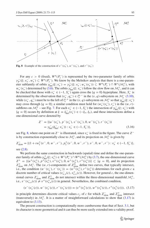
Fig. 8 Example of the construction of v−(v−∗ ), w−(v−∗ ), and r−(v−∗ )

For any c > 0 (fixed), W u(P−ε ) is represented by the two-parameter family of orbits

γ −P (ξ ; v−∗ , w−∗ ) ⊂ W u(P−

ε ). We know by the Melnikov analysis that there is a one-param-eter subfamily of orbits γ −

het(ξ ; v−∗ ) = γ −P (ξ ; v−∗ ;w−∗ (v−∗ )) ⊂ W u(P−

ε ) ∩ W s(M+ε ), with

w−∗ (v−∗ ) determined by (3.6). The orbits γ −het(ξ ; v−∗ ) follow the slow flow on M+

ε , and it canbe checked that those with v−∗ ∈ (−1, S−

v ) again cross the {q = 0}-hyperplane. Here, S−v is

determined by the observation that (v−∗ , q−∗ ) ∈ lu,−v in the (v, q)-subsystem on M−

ε (3.10),while (v−∗ , q−∗ ) must be to the left of ls,+

v in the (v, q)-subsystem on M+ε so that γ −

het(ξ ; v−∗ )

may cross through {q = 0}; a similar condition must hold for (w−∗ (v−∗ ), r−∗ ) in the (w, r)-subflows on M∓

ε – see Fig. 7. For each v−∗ ∈ (−1, S−v ) the intersection of γ −

het(ξ ; v−∗ ) with{q = 0} occurs by definition at ξ = ξ−

het(v−∗ ) ∈ (−ξ∗, ξ∗), and these intersections define a

one-dimensional curve denoted by

Z− = {(u−(v−∗ ), p−(v−∗ ), v−(v−∗ ), 0, w−(v−∗ ), r−(v−∗ ))

= γ −het(ξ

−het; v−∗ )) : v−∗ ∈ (−1, S−

v )}, (3.16)

see Fig. 8, where one point on Z− is illustrated, since v−∗ is fixed in the figure. The curve Z−is by construction exponentially close to M+

ε , and its projection on M+ε is given by

Z−slow = {(1 + εu+

1 (v−, 0, w−, r−), p+1 (v−, 0, w−, r−), v−, 0, w−, r−) : v−∗ ∈ (−1, S−

v )},see (2.8).

We perform the same construction in backwards (spatial) time and define the one-param-eter family of orbits γ +

het(ξ ; v+∗ ) ∈ W s(P−ε )∩ W u(M+

ε ) by (3.7), the one-dimensional curveZ+ = {(u+(v+∗ ), p+(v+∗ ), v+(v+∗ ), 0, w+(v+∗ ), r+(v+∗ ))} ⊂ {q = 0}, and its projectionZ+

slow on M+ε . The (w, r)-components of Z±

slow define two curves, that typically intersect,i.e., the condition (w−(v−∗ ), r−(v−∗ )) = (w+(v+∗ ), r+(v+∗ )) determines for each given c adiscrete number of critical values (v−∗,∗(c), v+∗,∗(c)). However, for general c, the one-dimen-sional curves Z−

slow and Z+slow do not intersect within the three-dimensional manifold M+

ε ,i.e., v−(v−∗,∗(c)) �= v+(v+∗,∗(c)) in general. Nevertheless, the combined condition,

(v−(v−∗ (c)), w−(v−∗ (c)), r−(v−∗ (c))) = (v+(v+∗ (c)), w+(v+∗ (c)), r+(v+∗ (c))), (3.17)

in principle determines discrete critical values c j of c for which Z−slow and Z+

slow intersect(transversely) in M+

ε . It is a matter of straightforward calculations to show that (3.17) isequivalent to (3.13).

The present construction is computationally more cumbersome than that of Sect. 3.1, butits character is more geometrical and it can thus be more easily extended into a validity proof.

123

96 J Dyn Diff Equat (2009) 21:73–115

To do so, we define (for any c) the special heteroclinic orbits γ −∗,∗(ξ ; c) = γ −het(ξ ; v−∗,∗) ⊂

W u(P−ε ) ∩ W s(M+

ε ) and γ +∗,∗(ξ ; c) = γ +het(ξ ; v+∗,∗) ⊂ W s(P−

ε ) ∩ W u(M+ε ). The tube

T −∗,∗(c) ⊂ W u(P−ε ) is spanned by those orbits γ −

P (ξ ; v−∗ , w−∗ ) ⊂ W u(P−ε ) that are exponen-

tially close to γ −∗,∗(ξ ; c) for ξ < 12 (−ξ∗+ξ−

het(v−∗,∗)). Likewise, the tube T +∗,∗(c) ⊂ W s(P−

ε ) isspanned by those orbits γ +

P (ξ ; v−∗ , w−∗ ) ⊂ W s(P−ε ) that are exponentially close to γ +∗,∗(ξ ; c)

for ξ > 12 (ξ∗ + ξ+

het(v+∗,∗)). In forwards ‘time’, T −∗,∗(c) is stretched along W u(M+

ε ), whileT +∗,∗(c) is stretched along W s(M+

ε ) in backwards ‘time’. By construction, the (stretched)tubes intersect the five-dimensional hyperplane {q = 0} in two-dimensional manifolds,Z±

T (c) (by definition).The theorem is proved if it can be established that there are non-zero values of c for

which Z−T (c) ∩ Z+

T (c) �= ∅, since each point in this intersection determines a point inW u(P−

ε ) ∩ W s(P−ε ) ∩ {q = 0}.

To show this, we extend {q = 0} to a six-dimensional space, denoted by {{q = 0}, c}, byadding c as an independent variable. This space contains the extended manifolds {Z−

T (c), c}and {Z+

T (c), c} as three-dimensional subsets. Since γ −∗,∗(ξ ; c) and γ +∗,∗(ξ ; c) are exponentiallyclose to M+

ε as they intersect {q = 0}, and since the projections Z−slow and Z+

slow intersect byconstruction near c = c j determined by (3.13), it follows that {Z−

T (c), c} and {Z+T (c), c} are

exponentially close for c near c j . As in the proof of Theorem 2.1, it now follows from the factthat T −∗,∗(c) is stretched along W u(M+

ε ) and T +∗,∗(c) along W s(M+ε ), that—in the six-dimen-

sional space {{q = 0}, c}—the three-dimensional manifolds {Z−T (c), c} and {Z+

T (c), c} mustintersect transversely in discrete points that have c-coordinates c∗

j (ε), which are to leading

order determined by (3.13) or (3.17). Hence, Z−T (c) ∩ Z+

T (c) = γ −tr, j (ξ) ∩ {q = 0} �= ∅ at

c∗j (ε) = c j + O(ε). ��

4 Bifurcation from Stationary to Travelling Pulse Solutions

4.1 Leading Order Analysis

To investigate the nature of the bifurcation from stationary one-pulse solutions to travellingone-pulse solutions, we start by considering the travelling pulse just after ‘creation’, that is,we set

c = δ, (4.1)

with 0 < ε � δ � 1 (so c is no longer an unknown anymore). We expand the threeunknowns, τ = τ∗,0 + O(δ), θ = θ∗,0 + O(δ), ξ∗ = ξ∗,0 + δξ∗,1 + O(δ2). Notice that τ∗,0

and θ∗,0 determine the bifurcation values of τ and θ at which the bifurcation occurs, sincethe speed of the bifurcating travelling pulse reduces to zero at τ = τ∗,0 and θ = θ∗,0. Sincethe bifurcation is co-dimension one we expect to find a relation between τ∗,0 and θ∗,0.

The eigenvalues (3.8) and (3.12) become

λ±v = ±1 − 1

2τ∗,0δ + O(δ2), λ±

w = ± 1

D− 1

2

θ∗,0

D2 δ + O(δ2),

s±v = −1 ± 1

2τ∗,0δ + O(δ2), s±

w = −1 ± 1

2

θ∗,0

Dδ + O(δ2).

123

J Dyn Diff Equat (2009) 21:73–115 97

20 40 60 80 100

0.25

0.5

0.75

1

1.25

1.5

Fig. 9 For (α, β, γ, ε) = (3, 1, 2, 0.01), the bifurcation point τ∗,0(θ∗,0) is plotted for D = 2, 5, 10, 100. Thevalue of the jump mid-point ξ∗,0 is, respectively, 40.547, 47.018, 50.356, 54.393 and is computed through(4.2). When D = ∞, we have ξ∗,0 = 54.931 and τ∗,0(θ∗,0) = τ∗,0 = 1.0460. This is the dotted line in thefigure

We also expand the four equalities in (3.11), using A0 := e−εξ∗,0 ,

v±∗ = −A20 ∓ τ∗,0δ

(1

2− 1

2A2

0 + A20 log A0

)

+ 2εξ∗,1 A20δ + O(δ2),

w±∗ = −A2D0 ∓ θ∗,0

Dδ

(1

2− 1

2A

2D0 + 1

DA

2D0 log A0

)

+ 2ε

Dξ∗,1 A

2D0 δ + O(δ2).

Next, we substitute the above expansions into the jump condition (3.13), and we recall thatc = δ, to obtain

⎧⎪⎪⎪⎪⎨

⎪⎪⎪⎪⎩

γ = αA20 + β A

2D0 (twice),

13

√2 = ατ∗,0

( 12 − 1

2 A20 + A2

0 log A0)+ β

θ∗,0D

(12 − 1

2 A2D0 + 1

D A2D0 log A0

)

,

0 = 4εξ∗,1

(

αA20 + β

D A2D0

)

,

(4.2)

where we equated coefficients on O(1) and O(δ) terms, respectively, and added and sub-tracted the two O(δ) equations. Note that the equation for A0 is identical to that of thestationary one-pulse orbit (2.22): near the bifurcation the width of the travelling pulse is toleading order equal to that of the stationary pulse. Equation 4.2 determine the three unknownsA0 (which gives ξ∗,0), τ∗,0 as function of θ∗,0, and ξ∗,1 = 0. The solution τ∗,0 as function ofθ∗,0, is plotted in Fig. 9 for several values of D.

Remark 4.1 We briefly consider the case of D large, i.e., D = O( 1δ). It immediately follows

from (4.2) that ξ∗,0 = − 12

1ε

log(

γ−βα

). (Here, we also have to assume that γ > β, α > 0 or

that γ < β, α < 0). Moreover,

τ∗,0(θ) = 2

3

√2

(

α − (γ − β) + (γ − β) log

(γ − β

α

))−1

+ O(δ).

This τ∗,0 is analogous to the (τ2)∗,0 we find in the analysis for travelling pulses of the reducedtwo-component system (6.1)—see Sect. 6.

123

98 J Dyn Diff Equat (2009) 21:73–115

4.2 Subcriticality and Supercriticality of the Bifurcation

To determine the nature (supercritical versus subcritical) of the bifurcation, see Fig. 11, andalso for the stability analysis [23], we actually need the correction terms up to and includingthird order in δ in the above calculations. To keep the calculations within reasonable limits,we set the bifurcation parameter θ equal to one, such that in the above analysis the w-com-ponent is symmetric and has no higher order corrections, i.e., θ = 0 in (3.8), etc. Note that θ

has also been set to θ = 1 in [17,24,25]. Moreover, most of the numerical results presentedin [2,15,18,22] are for θ = 1. We also assume that αA2

0 + βD A2/D

0 > 0, which implies thatthe stationary one-pulse limit is not near a saddle-node bifurcation and that it is stable [23].

Lemma 4.1 Let (α, β, γ, D, τ, θ, ε) be such that τ = O( 1ε2 ), θ = 1, α > 0, (2.22) holds,

and αA20 + β

D A2/D0 > 0, where A0 = e−εξ∗,0 and 0 < ε � 1. For c = δ, with ε � δ � 1, a

travelling pulse exists for τ = 1ε2 (τ∗,0 + δ2τ∗,2 + O(δ3)), with

τ∗,0 = 2

3

√2

1

α(1 − A20 + A2

0 log A20)

> 0,

τ∗,2 = 3

32

√2α(τ∗,0)

4[

1 − A20 + A2

0 log A20 − 1

3A2

0 log3 A20

+αA40 log2 A2

0(log A20 − 1)

αA20 + β

D A2/D0

]

. (4.3)

Note that the sign of τ∗,2 determines the nature of the bifurcation: a negative τ∗,2 yields a sub-critical bifurcation, while a positive τ∗,2 yields a supercritical bifurcation. For given systemparameters, we can evaluate (4.3) to determine the sign of τ∗,2. Moreover, we observe thatit is possible for the same (α, β, D) for τ∗,2 to take on positive, as well as negative, values,depending on γ (via A0), as is illustrated in Fig. 10.

Proof The proof consists of an elaborate—but straightforward—asymptotic analysis of thejump conditions (3.13). Plugging in v±∗ , w±∗ with θ = 1 yields, to leading order in ε,

α(s±v (e±2ελ∓

v ξ∗ − 1) − 1) − βe−2 εD ξ∗ + γ = ∓1

3

√2c.

0.2 0.4 0.6 0.8 1-0.2

0.2

0.4

0.6

0.8

1 0.2 0.4 0.6 0.8 1

-10

-8

-6

-4

-2

Fig. 10 Left frame: (α, β, D) = (3, 1, 5). Right frame: (α, β, D) = (3, −1, 5). Note that we did not plot τ∗,2

but a ‘scaled’ version τ∗,2/C . To be more precise, C = 332

√2α(τ∗,0)4, and the scaling therefore depends on

A0. However, C > 0 for A0 ∈ (0, 1). Thus, the scaling does not change the sign of τ∗,2. Moreover, note that

the vertical asymptote (for β < 0) is exactly where αA20 + β

D A2D0 = 0 (A0 = Ac , see (2.25)). The last free

parameter, γ , actually determines the value of A0 via (4.7). Thus for (α, β, D) = (3, 1, 5) it is possible tohave a negative, as well as a positive τ∗,2

123

J Dyn Diff Equat (2009) 21:73–115 99

After expanding the two unknown variables τ and ξ∗,

τ=τ∗,0+δτ∗,1+δ2τ∗,2 + δ3τ∗,3 + O(δ4), ξ∗ = ξ∗,0 + δξ∗,1 + δ2ξ∗,2 + δ3ξ∗,3 + O(δ4),

we obtain the leading order approximations of (3.8) and (3.12),

λ±v = ±1 − 1

2τ∗,0δ +

(

±1

8τ 2∗,0 − 1

2τ∗,1

)

δ2 +(

±1

4τ∗,0τ∗,1 − 1

2τ∗,2

)

δ3 + O(δ4),

s±v = −1 ± 1

2τ∗,0δ ± 1

2τ∗,1δ

2 ∓(

1

16τ 3∗,0 − 1

2τ∗,2

)

δ3 + O(δ4). (4.4)

With these expressions we deduce

e±2ελ∓v ξ∗ = e−2εξ∗,0+e−2εξ∗,0(∓ετ0ξ∗,0−2εξ∗,1)δ+e−2εξ∗,0 [−1

4ε(τ∗,0)

2ξ∗,0 ∓ ετ∗,1ξ∗,0

∓ετ∗,0ξ∗,1 ± 2ε2τ∗,0ξ∗,0ξ∗,1 + 1

2ε2(τ∗,0)

2(ξ∗,0)2 + 2ε2(ξ∗,1)

2 − 2εξ∗,2]δ2

+e−2εξ∗,0

[

−1

2ετ∗,0τ∗,1ξ∗,0 ∓ ετ2ξ∗,0 ± 1

4ε2(τ∗,0)

3(ξ∗,0)2+ε2τ∗,0τ∗,1(ξ∗,0)

2

∓1

6ε3(τ∗,0)

3(ξ∗,0)3 − 1

4ε(τ∗,0)

2ξ∗,1 ∓ ετ∗,1ξ∗,1 + 3

2ε2(τ∗,0)

2ξ∗,0ξ∗,1

±2ε2τ∗,1ξ∗,0ξ∗,1 − ε3(τ∗,0)2(ξ∗,0)

2ξ∗,1 ± 2ε2τ∗,0(ξ∗,1)2 ∓ 2ε3τ∗,0ξ∗,0(ξ∗,1)

2

−4

3ε3(ξ∗,1)

3 ∓ ετ∗,0ξ∗,2 ± 2ε2τ∗,0ξ∗,0ξ∗,2+4ε2ξ∗,1ξ∗,2−2εξ∗,3

]

δ3+O(δ4),

(4.5)

and

e−2 εD ξ∗ = e−2 ε

D ξ∗,0 − 2

Dεξ∗,1e−2 ε

D ξ∗,0δ + e−2 εD ξ∗,0

[2

D2 ε2(ξ∗,1)2 − 2

Dεξ∗,2

]

δ2

+e−2 εD ξ∗,0

[

− 4

3D3 ε3(ξ∗,1)3 + 4

D2 ε2ξ∗,1ξ∗,2 − 2

Dεξ∗,3

]

δ3 + O(δ4). (4.6)

(Recall that εξ∗, j = O(1).)Combining (4.4), (4.5), and (4.6), we find to leading order (twice)

αA20 + β A

2D0 = γ, (4.7)

which agrees with the first equation in (4.2).The O(δ) corrections read

±1

2ατ∗,0(1 − A2

0 + A20 log A2

0) + 2εξ∗,1(αA20 + β

DA

2D0 ) = ±1

3

√2.

By adding and subtracting the above two equations, we obtain

ξ∗,1 = 0, τ∗,0 = 2

3

√2

1

α(1 − A20 + A2

0 log A20)

,

which agrees with (4.2), since θ∗,0 = 0. Note that the function 1− A20 + A2

0 log A20 is positive

for all A0 ∈ (0, 1) – it decreases monotonically from one to zero as A0 increases from zeroto one. Since α > 0 it follows that τ∗,0 > 0.

123

100 J Dyn Diff Equat (2009) 21:73–115

At O(δ2), we find

0 = ±1

2ατ∗,1(A2

0 − 1) − αA20

[

−1

4ε(τ∗,0)

2ξ∗,0 ∓ ετ1ξ∗,0 + 1

2ε2(τ∗,0)

2(ξ∗,0)2 − 2εξ∗,2

]

−1

2εα(τ∗,0)

2ξ∗,0 A20 + 2

β

Dεξ∗,2 A

2D0 ,

(since ξ∗,1 = 0). Subtracting the two equalities implies

ατ∗,1(1 − A20 + A2

0 log A20) = 0 ⇒ τ∗,1 = 0.

Adding both terms yields

ξ∗,2 = 1

16

1

ε

αA20(τ∗,0)

2 log A20(log A2

0 − 1)

αA20 + β

D A2/D0

.

We note that log A20 − 1 < log A2

0 < 0 and αA20 + β

D A2/D0 > 0, therefore, sgn(ξ∗,2) =

sgn(α) = +1. Thus, the width of the pulse (2ξ∗) is larger than the leading order width(2ξ∗,0), i.e., the width of the travelling pulse is larger than the width of the standing pulse.

The O(δ3)-term is given by

0 = ±α

(1

16(τ∗,0)

3 − 1

2τ∗,2

)

(A20 − 1) ∓ 1

2ατ∗,0 A2

0

[

− 1

4ε(τ∗,0)

2ξ∗,0

+1

2ε2(τ∗,0)

2(ξ∗,0)2 − 2εξ∗,2

]

∓αA20[ετ∗,2ξ∗,0 − 1

4ε2(τ∗,0)

3(ξ∗,0)2 + 1

6ε3(τ∗,0)

3(ξ∗,0)3

+ετ∗,0ξ∗,2 − 2ε2τ∗,0ξ∗,0ξ∗,2 ∓ 2εξ∗,3]

+2β

Dεξ∗,3 A

2D0 .

Adding both terms implies ξ∗,3 = 0, subtracting yields,

α

(1

16(τ∗,0)

3 − 1

2τ∗,2

)

(A20 − 1) − 1

2ατ∗,0 A2

0

[

− 1

4ε(τ∗,0)

2ξ∗,0 + 1

2ε2(τ∗,0)

2(ξ∗,0)2

−2εξ∗,2

]

− αA20

[

ετ∗,2ξ∗,0 − 1

4ε2(τ∗,0)

3(ξ∗,0)2 + 1

6ε3(τ∗,0)

3(ξ∗,0)3 + ετ∗,0ξ∗,2

−2ε2τ∗,0ξ∗,0ξ∗,2

]

= 0,

which can be rewritten as

0 = −αA20τ∗,0εξ∗,2 log A2

0 + 1

48αA2

0(τ∗,0)3 log3 A2

0 − 1

16α(τ∗,0)

3(1 − A20 + A2

0 log A20)

+1

2ατ∗,2(1 − A2

0 + A20 log A2

0).

123

J Dyn Diff Equat (2009) 21:73–115 101

Then, using the expression for τ∗,0 and ξ∗,2, we obtain

τ∗,2 = 1

8(τ∗,0)

3 − 1

32

√2αA2

0(τ∗,0)4 log3 A2

0 + 3

32

√2α2 A4

0(τ∗,0)4 log2 A2

0(log A20 − 1)

αA20 + β

D A2/D0

,

(4.8)

which can be rewritten as in (4.3). ��

For D large, we can analytically determine the sign of τ∗,2 in (4.3), as we now show.

Corollary 4.2 Let (α, β, γ, D, τ, θ, ε) and A0 be as in Lemma 4.1 and assume that D = 1δ

with 0 < ε � δ � 1. Define AZ0 ∈ (0, 1) as the (unique) solution of

1 − A20 + A2

0 log A20 + 2

3A2

0 log3 A20 − A2

0 log2 A20 = 0, (4.9)

(AZ0 = 0.11063 . . .). Then, τ∗,2 > 0 for parameter combinations such that 0 < A0 <

AZ0 + O(δ) and τ∗,2 < 0 for 1 > A0 > AZ

0 + O(δ).

Proof It follows from (4.3) that, to leading order in δ,

τ∗,2|D=O(δ−1) = 3

32

√2α(τ∗,0)

4[

1 − A20 + A2

0 log A20

−1

3A2

0 log3 A20 + A2

0 log2 A20(log A2

0 − 1)

]

= 3

32

√2α(τ∗,0)

4[

1 − A20 + A2

0 log A20 + 2

3A2

0 log3 A20

−A20 log2 A2

0

]

=: C τ′∗,2,

with C = 332

√2α(τ∗,0)

4 > 0 and τ′∗,2 = 1 − A2

0 + A20 log A2

0 + 23 A2

0 log3 A20 − A2

0 log2 A20.

Thus sgn(τ∗,2) = sgn(τ′∗,2). We notice that τ

′∗,2(0) = 1 and τ

′∗,2(1) = 0. We now show that

τ′∗,2(s), with s := A2

0, has a negative minimum by differentiating,

d

dsτ

′∗,2 = (log s)

(2

3log2 s + log s − 1

)

.

Thus, with z := log s (so that z ∈ (−∞, 0)), we see that τ′∗,2(z) has a unique extremum if

23 z2 + z − 1 = 0, i.e., z = zM = − 3

4 − 14

√33. This implies that AM

0 = e− 18 (3+√

33) ∈ (0, 1),so that

τ′∗,2(AM

0 ) = 1 − e− 14 (3+√

33)

(31

4+ 5

4

√33

)

< 0.

Hence, AM0 determines a negative minimum of τ

′∗,2, which implies τ

′∗,2 must change sign

once for A = AZ0 ∈ (0, AM

0 ), where AZ0 is determined by (4.9). ��

An additional consequence of Lemma 4.1, that holds for more general values of D, is

Corollary 4.3 Let (α, β, γ, D, τ, θ, ε) and A0 be as in Lemma 4.1. Furthermore, assumethat β < 0, αD > −β, A0 > Ac > AZ

0 (with Ac, AZ0 as in (2.25), (4.9), respectively), then

the bifurcation is subcritical, i.e., τ∗,2 < 0.

123

102 J Dyn Diff Equat (2009) 21:73–115

2 4 6 8 10

2

4

6

8

5.96 5.98 6.02 6.04

0.01

0.02

0.03

0.04

Fig. 11 The solution curve of equation (3.13) in the (τ , c) plane for the parameter values (α, β, γ, D, θ, ε) =(5, −3, 1, 4, 1, 0.01). We have chosen the parameters in such a fashion that they satisfy the conditions inRemark 4.2. In the left frame we observe a subcritical bifurcation at τ = τ∗,0 = 6.01363. Moreover, weobserve that as τ goes to infinity the upperbranch, c+(τ ), goes to the theoretically predicted, leading ordervalue, 3

2

√2(α − γ ) = 6

√2, see (3.15). Finally, from this numerical continuation we observe that the two

branches merge at a saddle-node bifurcation at τnumSN = 0.84917 and cnum

SN = 6.3027. In the right frame, theregion near τ = τ∗,0 is magnified

Proof Observe that in this case

αA40 log2 A2

0(log A20 − 1)

αA20 + β

D A2/D0

< A20 log2 A2

0(log A20 − 1) < 0.

Therefore, τ∗,2(A0) < C τ′∗,2(A0), with τ

′∗,2(A0) as defined above, and C τ

′∗,2(A0) is negative

for A0 > AZ0 . ��

Remark 4.2 If, in addition to the conditions in Corollary 4.3, it is also assumed that α > γ ,then it follows from our analysis in Sect. 3.2 that there is a travelling pulse with speedc = 3

2

√2(α − γ )+O(δ, ε) > 0 for τ � 1 (3.15). This indicates that the curve c = c(τ ) has

a fold structure, i.e., for increasing τ (and all other parameters fixed) there is a saddle-nodebifurcation of travelling pulses at τ = τSN < τ∗,0 at which two travelling pulses bifurcatewith speeds c±(τ ) > 0 and c±(τSN ) = cSN > 0; the pulse associated to c−(τ ) mergeswith the stationary pulse at τ = τ∗,0, while the other pulse exists for all τ > τSN , so thatc+(τ ) → 3

2

√2(α − γ ) as τ → ∞. This can be checked by using a continuation method for

the solutions of (3.13), see Fig. 11. Hence, there exist parameter combinations for which twotypes of travelling pulses coexist with the stationary pulse (for τSN < τ < τ∗,0). Both thestationary pulse and the travelling pulse associated to c+(τ ) may be stable [23].

5 Stationary Two-Pulse Solutions

In this section, we establish the existence of localized, symmetric, standing, two-pulse solu-tions of (1.6). We construct these pulses as homoclinic orbits γ −

2p, j (ξ) to the critical point P−ε .

5.1 The Construction of γ −2p, j (ξ) Homoclinic to P−

ε

We search for stationary pulse-like solutions. Therefore, the PDE (1.7) again reduces to (2.1),and the basic observations (on the fixed points, the reduced limits, the slow manifolds, etc.)are the same as in Sect. 2.1. However, for symmetric standing two-pulse solutions, we have

123

J Dyn Diff Equat (2009) 21:73–115 103

to distinguish nine different regions instead of the five regions as we did for the one-pulsesolutions—see Sect. 2.2. We again parametrize the two-pulse solutions so that its u, v, w-components are at a local extremum at ξ = 0. However, there are three local extrema, seeFig. 1, and for symmetry considerations we choose to put the zero of the ξ -axis at the secondlocation, the one exponentially close to M−

ε . It turns out that v−2p, j (0) and w−

2p, j (0) are local

minima, while u−2p, j (0) is a local maximum, see Figs. 1 and 12. We define the four ‘jump

mid-points’ of γ −2p, j by ±ξ

1,2∗ (not to be confused with the ξ∗,1, ξ∗,2 of the previous sec-

tion). Where the last ‘back’ (i.e., the final jump of M+ε back to M−

ε ) of γ −2p, j (ξ) crosses the

{u = 0}-hyperplane at ξ = ξ1∗ , and the last front of γ −2p, j (ξ) crosses the same hyperplane at

ξ = ξ2∗ . Note that by construction 0 < ξ2∗ < ξ1∗ . The reversibility symmetry implies that −ξ1∗is the jump mid-point of the first front and −ξ2∗ is the jump mid-point of the first back. Thus,

γ −2p, j (±ξ1∗ ) = (0,∓p1∗, v1∗,∓q1∗ , w1∗,∓r1∗ ), γ −

2p, j (±ξ2∗ ) = (0,±p2∗, v2∗,±q2∗ , w2∗,±r2∗ ).

(5.1)

We assume that ξ1∗ , ξ2∗ , as well as ξ1∗ − ξ2∗ , are large, i.e., ξ1,2∗ and ξ1∗ − ξ2∗ are O( 1ε). We now

define the four fast intervals I 2,4,6,8f and the five slow intervals I 1,3,5,7,9

s

I 2,4f : =

(

−ξ1,2∗ − 1√ε,−ξ1,2∗ + 1√

ε

)

, I 6,8f :=

(

ξ2,1∗ − 1√ε, ξ2,1∗ + 1√

ε

)

,

I 1s : =

(

−∞,−ξ1∗ − 1√ε

]

, I 3,7s :=

[

∓ξ1,2∗ + 1√ε,∓ξ2,1∗ − 1√

ε

]

,

I 5s : =

[

−ξ2∗ + 1√ε, ξ2∗ − 1√

ε

]

, I 9s :=

[

ξ1∗ + 1√ε,∞

)

.

The nine different regions are then

1. The dynamics take place exponentially close to the slow manifold M−ε : ξ ∈ I 1

s .2. The dynamics take place in the fast field: ξ ∈ I 2

f .

3. The dynamics take place exponentially close to M+ε : ξ ∈ I 3

s .4. The dynamics take place in the fast field: ξ ∈ I 4

f .

5. The dynamics take place exponentially close to M−ε : ξ ∈ I 5

s .6. The dynamics take place in the fast field: ξ ∈ I 6

f .

7. The dynamics take place exponentially close to M+ε : ξ ∈ I 7

s .8. The dynamics take place in the fast field: ξ ∈ I 8

f .

9. The dynamics take place exponentially close to M−ε : ξ ∈ I 9

s .

The analysis of the formal construction is now nearly the same as for the standing one-pulsecase (Sect. 2.2); the only difference is that it involves a bit more bookkeeping. However,qualitatively, nothing changes; for example we still have

2,4,6,8f (v,w, q, r) = O(

√ε), the

equivalent of (2.15). The homoclinic v,w-component on the slow manifolds are still gov-erned by (2.10) and (2.11). Together with the usual boundary conditions, of which there arein total forty, we get

123

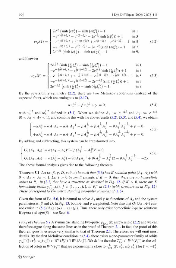
104 J Dyn Diff Equat (2009) 21:73–115

v2p(ξ) =

⎧⎪⎪⎪⎪⎪⎨

⎪⎪⎪⎪⎪⎩

2eεξ(sinh

(εξ1∗

)− sinh(εξ2∗

))− 1 in 1

−e−ε(ξ+ξ1∗ ) − eε(ξ−ξ1∗ ) − 2eεξ (sinh (εξ2∗ )) + 1 in 3

−e−ε(ξ+ξ1∗ ) + e−ε(ξ+ξ2∗ ) + eε(ξ−ξ2∗ ) − eε(ξ−ξ1∗ ) − 1 in 5

−e−ε(ξ+ξ1∗ ) − eε(ξ−ξ1∗ ) − 2e−εξ (sinh (εξ2∗ )) + 1 in 72e−εξ

(sinh (εξ1∗ ) − sinh (εξ2∗ )

)− 1 in 9,

(5.2)

and likewise

w2p(ξ) =

⎧⎪⎪⎪⎪⎪⎨

⎪⎪⎪⎪⎪⎩

2eεD ξ(sinh

(εD ξ1∗

)− sinh(

εD ξ2∗

))− 1 in 1

−e− εD (ξ+ξ1∗ ) − e

εD (ξ−ξ1∗ ) − 2e

εD ξ (sinh ( ε

D ξ2∗ )) + 1 in 3

−e− εD (ξ+ξ1∗ ) + e− ε

D (ξ+ξ2∗ ) + eεD (ξ−ξ2∗ ) − e

εD (ξ−ξ1∗ ) − 1 in 5

−e− εD (ξ+ξ1∗ ) − e

εD (ξ−ξ1∗ ) − 2e− ε

D ξ (sinh ( εD ξ2∗ )) + 1 in 7

2e− εD ξ(sinh ( ε

D ξ1∗ ) − sinh ( εD ξ2∗ )

)− 1 in 9.

(5.3)

By the reversibility symmetry (2.2), there are two Melnikov conditions (instead of theexpected four), which are analogous to (2.17),

αv1,2∗ + βw1,2∗ + γ = 0, (5.4)

with v1,2∗ and w

1,2∗ defined in (5.1). When we define A1 := e−εξ1∗ and A2 := e−εξ2∗(0 < A1 < A2 < 1), and combine this with the above results (5.2), (5.3), and (5.4), we obtain

⎧⎨

⎩

−αA21 + αA1 A2 − αA1 A−1

2 − β A2D1 + β A

1D1 A

1D2 − β A

1D1 A

− 1D

2 + γ = 0

+αA22 − αA1 A2 − αA1 A−1

2 + β A2D2 − β A

1D1 A

1D2 − β A

1D1 A

− 1D

2 + γ = 0.

(5.5)

By adding and subtracting, this system can be transformed into⎧⎨

⎩

G1(A1, A2) := α(A1 − A2)2 + β(A

1D1 − A

1D2 )2 = 0

G2(A1, A2) := α(A22 − A2

1) − 2αA1 A−12 + β(A

2D2 − A

2D1 )2 − β A

1D1 A

− 1D

2 = −2γ.

(5.6)

The above formal analysis gives rise to the following theorem.

Theorem 5.1 Let (α, β, γ, D, τ, θ, ε) be such that (5.6) has K solution pairs (A1, A2) with0 < A1 < A2 < 1. Let ε > 0 be small enough. If K = 0, then there are no homoclinicorbits to P−

ε in (2.1) that have a structure as sketched in Fig. 12. If K > 0, there are Khomoclinic orbits γ −

2p, j (ξ), j ∈ {1, . . . , K }, to P−ε in (2.1) (with structure as in Fig. 12).

These correspond to symmetric standing two-pulse solutions of (1.6).

Given the form of Eq. 5.6, it is natural to solve A1 and γ as functions of A2 and the systemparameters α, β and D. In Fig. 13, both A1 and γ are plotted. Note also that G1(A1, A2) can-not vanish in (5.6) if sgn(α) = sgn(β). Thus, there only exist homoclinic 2-pulse solutionsif sgn(α) �= sgn(β)—see Sect. 6.

Proof of Theorem 5.1 A symmetric standing two-pulse γ −2p, j (ξ) is reversible (2.2) and we can

therefore argue along the same lines as in the proof of Theorem 2.1. In fact, the proof of thistheorem goes in essence very similar to that of Theorem 2.1. Therefore, we will omit mostdetails. By the first Melnikov condition in (5.4), there exists a one-parameter family of orbitsγ

1,−het (ξ ; v1∗;w1∗(v1∗)) ∈ W u(P−

ε )∩ W s(M+ε ). We define the tube T −

1,∗ ⊂ W u(P−ε ) as the col-

lection of orbits in W u(P−ε ) that are exponentially close to γ

1,−het (ξ ; v1∗;w1∗(v1∗)) for ξ < −ξ1∗ .

123

J Dyn Diff Equat (2009) 21:73–115 105

Fig. 12 A schematic sketch of a symmetric two-pulse γ −2p, j (ξ) homoclinic to P−

ε

Fig. 13 In the left frame, A1 is plotted as function of A2 for several values of D. In the right frame, γ isplotted as function of A2 for the same values for D. The dashed curve represents the asymptotic behaviorfor D large and is given by (5.12). The two-pulse orbits are typically created or annihilated in a saddle-nodebifurcation—see Sect. 7, Fig. 15

All orbits in T −1,∗ approach M+

ε and follow the slow flow on M+ε for some ‘time’ (which may

be infinite), after which they take off parallel (and exponentially close to) W u(M+ε ). In other

words, near M+ε T −

1,∗ is strongly stretched along the direction of W u(M+ε ). It thus follows

by the application of the second Melnikov condition in (5.4) that T −1,∗ intersects W s(M−

ε );

the intersection T −1,∗ ∩W s(M−

ε ) is again two-dimensional, i.e., it consists of a one-parameterfamily of orbits ⊂ W u(P−

ε )∩W s(M−ε ). As in the proof of Theorem 2.1, it can now be shown

that there is a unique orbit γ2,−0,∗ (ξ) ⊂ T −

1,∗ ∩ W s(M−ε ) that is homoclinic to M−

ε such that

γ2,−0,∗ (0) ∈ {q = r = 0} – note that this also determines the position of the symmetry point

ξ = 0. Again, the algebra leading to the construction of γ2,−0,∗ (ξ) is equivalent to the above

analysis and yields at leading order (5.6). The existence of the 2-pulse homoclinic orbitsγ −

2p, j (ξ) now follows by arguments that are identical to those in Theorem 2.1. It is based

on the construction of the sub-tube T −2,∗ ⊂ T −

1,∗ around γ2,−0,∗ (ξ), its symmetrical counterpart

T +2,∗ around the orbit γ

2,+0,∗ (ξ) and the application of the reversibility symmetry. ��

Remark 5.1 In the proof presented above we have used that the jump mid-points v1,2∗ and

w1,2∗ satisfy certain constraints. In particular, v1∗ ∈ (−1, 0), w1∗ = − 1

β(αv1∗+γ ), v2∗ ∈ (v1∗, V )

and w2∗ = − 1β(αv2∗ + γ ), where V = − ξ1∗ +ξ2∗

2 − 12ε

log(

1 − e−2εξ2∗ + e−ε(ξ1∗ +ξ2∗ ))

. These

123

106 J Dyn Diff Equat (2009) 21:73–115

constraints arise naturally from the requirement that the tracked orbits lie on the correct side ofthe stable and unstable manifolds of the slow manifold, so that they can have a second pulse.

Remark 5.2 In our analysis we have focused on the existence of localized one- and two-pulse patterns. As for instance in [4], the same geometrical approach as in the proofs ofTheorems 2.1, 3.1 and 5.1 can be applied to establish the existence of many other kinds ofstationary or travelling patterns, such as N -pulse solutions and various kinds of spatiallyperiodic wave trains. We refrain from going into the details here. However, we do noticethat these patterns can be stable and do play an important role in the dynamics of (1.7) – seesection 7.1 and especially Fig. 15.

5.2 The Existence of Two-Pulse Solutions

Just as was the case for the K of Theorem 2.1, it is, a priori, not clear whether there existparameter combinations for which the K of Theorem 5.1 is non-zero. To show that theseparameter regimes do exist we first choose an explicit D as an example, that is, we putD = 2. Naturally, we also have to assume sgn(α) �= sgn(β). With this special choice of Dwe analyze (5.6). It transforms into

{H1(A1, A2) := α(A1 − A2)

2 + β(√

A1 − √A2)

2 = 0

H2(A1, A2) := α(A22 − A2

1) − 2α A1A2

+ β(A2 − A1) − 2β

√A1A2

= −2γ.(5.7)

Observe that the equality H1(A1, A2) = 0 does not depend on γ . Moreover, γ only appearsin the right hand side of H2(A1, A2) = −2γ . That is, γ only shifts H2(A1, A2) up or down.So, instead of solving for A1 and A2 in terms of the unknown parameters α, β and γ , it ismuch easier to fix α, β and A2 and to determine A1 and γ such that (5.7) is solved. Actually,by doing so, we impose, alongside α and β, one of the jump mid-points ξ2∗ and try to locate thesecond jump mid-point ξ1∗ and γ such that (1.7) possesses a standing two-pulse. Of course,we could also choose to start with α, β, and A1 and determine A2 and γ that satisfy (5.7).

The zero of H1(A1, A2), for which 0 < A1 < A2, is given by the relation√

A1 +√A2 = √−β/α. (5.8)

When we implement this into formula (5.7) for H2(A1, A2) we find, after some manipulation,a unique γ :

γ = α − 2α(1 + A22)

√

− β

αA2− β

(

1 + 3A2 + 1

A2−√

− A2β

α−√

− β

αA2

)

. (5.9)

However, there are also restrictions on the choice of A2. We need 0 < A1 < A2 < 1.Therefore,

− 1

4

β

α< A2 < min

{

−β

α, 1

}

. (5.10)

We conclude that if A2 satisfies (5.10), there is a (α, β, γ )-parameter combination such that(5.7) is satisfied, i.e., such that a two-pulse solution exists. However, if (5.10) cannot besatisfied – which is the case when |4α| < |β|, there are no such two-pulse solutions.

This nonexistence result can be generalized to all D > 1:

Corollary 5.1 Let sgn(α) �= sgn(β). There is an open region in (α, β, γ, D)-space for whichhomoclinic two-pulse solutions as described in Theorem 5.1 exist. However, if |α|D2 < |β|,then there are no such two-pulse solutions.

123

J Dyn Diff Equat (2009) 21:73–115 107

Proof We start again by observing that G1(A1, A2) = 0 does not depend on γ , and that theγ in G2(A1, A2) = −2γ only shifts G2(A1, A2) up or down. So, again instead of solvingA1 and A2 in terms of α, β and γ via (5.6), we solve this equation for given α, β and A2

with the unknown parameters A1 and γ .The condition 0 < A1 < A2 < 1 yields the following generalization of (5.10)

(

− β

αD2

) 12

DD−1

< A2 < min

{(

−β

α

) 12

DD−1

, 1

}

. (5.11)

Here, the latter inequality ensures A2 ∈ (0, 1), and the former implies A1 < A2. This intervalis empty when |α|D2 < |β|. ��5.3 Asymptotics for D → ∞

In this section, we analyze the large D asymptotics of solutions of equation (5.6). FromFig. 13, we observe that, over a large portion of the interval A2 ∈ (0, 1), the solution curvesfor A1 lie near the axis, and the solution curves for γ lie near the lower dashed curve. More-over, these curves approach their respective asymptotes as D increases. We establish thisresult precisely in the following lemma:

Lemma 5.2 Assume that α > 0 > γ > β. Then, for strictly O(1) values of A2 ∈(0,

√−β/α), as measured with respect to the asymptotically small parameter 1/D, thesolutions A1 = A1(α, β, A2, D) and γ = γ (α, β, A2, D) of Eq. 5.6 satisfy, to leading order,

A1 =(

1 −√

−α

βA2

)D

, γ = −α

(√

−β

α− A2

)2

as D → ∞. (5.12)

The lower dashed curve in the right frame of Fig. 13 is this parabola of γ as function of A2.It is also useful to combine the results of (5.12) of this lemma into expressions for A1 andA2 in terms of the given system parameters. The result is, to leading order,

A1 =(

γ

β

) D2

, A2 =√

−β

α−√

−γ

α.

We also remark that in both frames there is a boundary layer at A2 = A1, which is why werequire A2 to be strictly of O(1) for this result and we recall that the existence constructionrequires that A1 < A2. In the boundary layer, the graph of A1 limits on the diagonal, witha slope of −1, while the graph of γ is nearly vertical. Although the asymptotic analysis isnot too involved, we refrain from going into the details here. Nevertheless, we notice that,by (5.6), γ = α + β in the limit A2 ↓ A1, see Fig. 13.

Proof of Lemma 5.2 We observe that, for A2 strictly of O(1) in (0,1), we may assume that

A1 = C D, (5.13)

to leading order, for some C ∈ (0, 1). Indeed, if one instead assumed that A1 = aδσ toleading order, for δ = 1/D and for some σ > 0, then from the first equation in (5.6) onewould find that A2 = 0 to leading order, which is a contradiction. Hence, with the assumption(5.13), the first equation in (5.6) becomes

αA22 + β(C − 1)2 = 0,

123

108 J Dyn Diff Equat (2009) 21:73–115

to leading order, where we used that A1/D2 = 1 + O(1/D) for A2 ∈ (0, 1), and that

(1/D) log(A2) � C . Solving, one finds, to leading order,

A1 =(

1 −√

−α

βA2

)D

, (5.14)

which is precisely the first formula of (5.12).With the asymptotics for A1 in hand, one may use the second formula in (5.6) to find the

asymptotics for γ . To leading order,

γ = −1

2

[

αA22 + β

(

1 −(

1 −√

−α

βA2

)2)

− 2β

(

1 −√

−α

βA2

)]

.

Simplifying the right member, we find precisely the asymptotic result (5.12) for γ . ��To conclude this section on the large D asymptotics, we comment briefly on the form of

the W profile for stationary two-pulse solutions in the interval between the two pulses. Fromthe above asymptotics, we find, to leading order,

εξ = O(1), εξ2∗ = − log A2 = O(1), εξ1∗ = −D log

(

1 −√

−α

βA2

)

= O(D).

(5.15)

Hence, from (5.3), we find in region 5, to leading order,

w2p(ξ) = −e− εD (ξ+ξ1∗ ) + e− ε

D (ξ+ξ2∗ ) + eεD (ξ−ξ2∗ ) − e

εD (ξ−ξ1∗ ) − 1

= 2√

−α

βA2 − 1

= 1 − 2√

γ

β. (5.16)

Therefore, for each A2 ∈ (0,√−β/α), the W -component is constant to leading order, where

the constant is given by (5.16). Moreover, we observe that W takes on all of the values in theinterval (−1, 1), since the above analysis applies for all A2 ∈ (0,

√−β/α).A stability analysis similar to that presented in [23] shows that the two-pulse solutions are

stable for parameter combinations in the ‘boundary layer’. However, they are unstable forparameter values near the dashed curve in the asymptotic regime studied in Lemma 5.2.

6 The Two-Component Model

In this section, we investigate the two-component (U, V )-subsystem of the three-componentmodel, that is, we send D to infinity and assume that the W -component is constant at W = −1everywhere in the PDE (1.6). The PDE model reduces to

{Ut = ε2Uxx + U − U 3 − ε(α2V + γ2)

τ2Vt = Vxx + U − V,(6.1)

with the same assumptions as before, 0 < ε � 1, 0 < τ2 � 1/ε3 and α2, γ2 ∈ R. Note thatthe notation for the parameters has the following correspondence with the parameters of thethree-component model: α2 = α, τ2 = τ and γ2 = γ − β.

123

J Dyn Diff Equat (2009) 21:73–115 109

It can be shown with the same techniques used in this article that for τ2 = O(1) the two-component system has standing one-pulse solutions homoclinic to P−

2,ε = (u−2,ε, 0, u−

2,ε, 0)

with u−2,ε = −1 + 1

2ε(α2 − γ2) + O(ε2) if there exists an A ∈ (0, 1) satisfying

α2 A2 = γ2 + O(√

ε),

recall (2.22). Hence, we immediately observe that necessary conditions for a standing pulsehomoclinic to P−

2,ε to exist are that sgn(α2) = sgn(γ2) and 0 < |γ2| < |α2|. Also,

the existence of travelling pulse solutions to P−2,ε for large τ2 can be proved, and in the

end it boils down to solving a system of equations which is a simplification of (3.13).Moreover, when we increase τ2 from an O(1)-parameter to an O(ε−2)-parameter a trav-elling pulse solution bifurcates from a standing pulse solution at (τ2)0,∗ = 1

ε2 (τ2)0,∗ =1ε2

23

√2(α2 − γ2 + γ2 log

(γ2α2

)). This bifurcation can be supercritical, as well as subcriti-

cal. See also Sect. 4 and especially the proof of Lemma 4.2.Finally, the two-component system possesses no symmetric standing two-pulse solutions

to P−2,ε. Physically, this can be explained by the fact that the model has too few free constants

(too few dimensions). The absence of two-pulse solutions is also plausible when we look atTheorem 5.1. There only exists a standing two-pulse solution if at least sgn(α) �= sgn(β)

and for the two-component system this condition cannot be fulfilled because there is noequivalent parameter for β in the two-component system.

To summarize, we have shown that the two-component model also possesses stationaryand travelling pulse solutions. However, it does not support two-pulse solutions.

Remark 6.1 There are two ways in which the three-component system (1.6) may limit on atwo-component system, either by considering W → V , associated to D ↓ 1, or by W → W0,a constant when D → ∞. In the former case one has to make the additional assumptionthat τ = θ . Since in most studies of systems like (1.1)/(1.6) D � 1 and τ � θ , we do notconsider this limit here.

If one considers the limit D → ∞ in Theorems 2.1 and 3.1 for one-pulse solutions, then itimmediately follows that W → −1 uniformly on R – see for instance (2.21). However, sincethe two-component limit cannot have standing two-pulse solutions, taking the limit D → ∞in Theorem 5.1 is less straightforward. In fact, this limit has already been discussed in section5.3 (under the assumption that A2 = O(1)). It follows from (5.15) that the width of the pulsesin the two-pulse solution increases linearly with D, while the distance between the pulsesapproaches a finite limit. Thus, on bounded intervals, the two-pulse solution of the three-com-ponent system limits on a one-pulse solution of a two-component (U, V )-system that is ho-moclinic to (U, V ) = (+1,+1) (with W → 1−2

√γ /β, the constant value given in (5.16)).

7 Simulations, Conclusions and Discussion

7.1 Simulations

In this section, we show the results of some numerical simulations to further illustrate thetheory presented in this article and also to illustrate some of the basic pulse interactions andinstabilities. These simulations are carried out using the numerical software presented in [1].

We already illustrated a stationary one-pulse solution in the left frame of Fig. 1. There-fore, we begin here with some travelling pulses of the type constructed in Sect. 3. Thepulses shown in Fig. 14 exist for values of τ greater than the theoretically predicted value

123

110 J Dyn Diff Equat (2009) 21:73–115

Fig. 14 Stable travelling pulses. The parameter values are (α, β, γ, D, θ, ε) = (6, 3, 4, 2, 1, 0.1), and τ is thebifurcation parameter. Here, we plotted a bouncing travelling pulse solution for τ = 110 and an annihilationof a travelling pulse for τ = 115

τ∗,0 = 0.59 for the bifurcation in which travelling pulses are created (which translates intoan unscaled τ∗,0 = 59). In the left frame, the travelling pulse collides with its mirror imagepulse at the boundary, since the boundary conditions are of homogeneous Neumann type,and afterwards they repel each other. By contrast, in the right frame, the pulse and its mirrorimage collide and then annihilate. The changeover from repulsion to annihilation after thecollision occurs at τ num

ann = 112. Finally, we observe that the numerically observed value ofthe bifurcation to travelling waves is τ num∗ = 103, which is within the relative error of mag-nitude O(1/ε) = O(10) of the leading order theoretical value τ∗,0 = 59. Of course, in thesesimulations ε is not yet really small, and hence we checked that the value of τ num∗ decreasestoward the value predicted by the leading order theory as ε is decreased. For example, forε = 0.01, we find τ num∗ = 5.95 × 103 (compared to 5.9 × 103 theoretically).

Next, we illustrate the theoretical results for stationary two-pulse solutions of (1.6), asderived in Sect. 5. For each of the four values of γ = 0.8, 0.75,−0.25,−0.3, Fig. 15 showsthe corresponding stationary solution. Based on the simulations for these parameter values, wefind that the homogeneous background state U = −1 undergoes a subcritical bifurcation intoa two-pulse solution at γ num = 0.78. Likewise, due to the reversibility symmetry, the homo-geneous state U = +1 bifurcates supercritically into a two-pulse solution at γ num = −0.78,though we do not show this. In addition, we observe that, as we decrease γ from 0.78, thewidth of the pulses increases, until there is a bifurcation at γ num = −0.27 at which the pulsescoalesce, and the solution is U = +1 everywhere, except inside an interior layer and insidethe layers at the boundaries of the computational interval. This solution is a spatially periodicsolution. Moreover, the observed value for this coalescence of the pulses agrees well with thetheoretically predicted value of γ = −0.31 for the saddle-node bifurcation, which occurs atthe minimum in the curve shown in the right frame of Fig. 13.

One of the most commonly-encountered bifurcations that the pulse solutions undergo is asupercritical Hopf bifurcation in which the widths, and heights, of the pulses oscillate peri-odically in time. In Fig. 16, we show a breathing one-pulse in the left frame, and a breathingtwo-pulse in the right frame. For the one-pulse solution (with ε = 0.1), the Hopf bifurca-tion occurs at τ num

H = 47. Moreover, we find that the breather dies out for τ = 49.8. For

123

J Dyn Diff Equat (2009) 21:73–115 111

−1000 −800 −600 −400 −200 0 200 400 600 800 1000

−1

−0.8

−0.6

−0.4

−0.2

0

0.2

0.4

0.6

0.8

1

−1000 −800 −600 −400 −200 0 200 400 600 800 1000

−1

−0.8

−0.6

−0.4

−0.2

0

0.2

0.4

0.6

0.8

1

−1000 −800 −600 −400 −200 0 200 400 600 800 1000

−1

−0.8

−0.6

−0.4

−0.2

0

0.2

0.4

0.6

0.8

1

−1000 −800 −600 −400 −200 0 200 400 600 800 1000

−1

−0.8

−0.6

−0.4

−0.2

0

0.2

0.4

0.6

0.8

1

Fig. 15 Plots of the stationary solutions of the three-component model (1.6) for four values of γ : γ =0.8, 0.75,−0.25,−0.3. The values of the other parameters are (α, β, D, τ, θ, ε) = (2, −1, 5, 1, 1, 0.01)

the two-pulse solution (with ε = 0.01), the Hopf bifurcation takes place at τ numH,2p = 4590.

Moreover, at τ = 5060, the breathing two-pulse solution becomes unstable and dies out. Wenote that we have observed breathing two-pulse solutions for which the pulse widths breathin an antisymmetric manner.

Scattering of pulses is also observed in the three-component model (1.7). In the left frameof Fig. 17, we show the V -component of a two-pulse solution in which the pulses initiallyapproach each other, spend a substantial amount of time at a nearly constant distance fromeach other with a significantly-decreased amplitude, and then regain their original amplitudesand repel each other. The pulses continue to repel each other until they reflect off the bound-ary, and the process repeats. A similar phenomenon has been observed in [15,16]. There theunstable, stationary two-pulse, which the two-pulse data approaches, is called a ‘scattor’ (or‘separator’). The importance of a scattor stems from the observation made in [15,16] thatthe forward evolution of two-pulse data that approaches it is determined by where that datalies with respect to the stable and unstable manifolds of the scattor or separator solution. Therelation between scattors and the two-pulse solutions constructed in this article is the subjectof future investigation.

We emphasize that the time interval shown in Fig. 17 is long and that the length of timewhere the two pulses are near to each other is also long in comparison to the time intervalover which the pulses move an O(1) distance. Moreover, we found that the duration of this

123

112 J Dyn Diff Equat (2009) 21:73–115

Fig. 16 Stable breathing one-pulse and two-pulse solutions. For the simulation shown in the left frame,τ = 49.7, and the other parameters are (α, β, γ, D, θ, ε) = (6, 3, 4, 10, 1, 0.1). Also, we note that the intervalused in the simulation is ξ ∈ [−100, 100], however we have displayed only a subinterval to better displaythe breathing behavior. For the simulation shown in the right frame, τ = 5000, and the other parametersare (α, β, γ, D, θ, ε) = (2.2, −1, 0, 10, 1, 0.01). Also, we note that the interval used in the simulation isξ ∈ [−1000, 1000]

Fig. 17 Scattering of two pulses. In the left frame, we show the V -component over a long time interval,and in the right frame we show the U -component during the third central scattering event (not shown for theV -component). The parameter values are (α, β, γ, D, τ, θ, ε) = (6, 3, 2, 2, 6500, 1, 0.01)

time interval can be changed by varying the parameter values. Finally, it is worth notingthat, during the time that the two pulses are near the boundaries, they are also near theircounterparts across the boundary, in what also appears to be a scattor state.

To conclude this brief section illustrating some of the pulse dynamics, we show the spatio-temporal evolution of four-pulse initial data in Fig. 18. Initially, the four pulses approach eachother. Then, they start to breath in a time-periodic manner, until finally the middle two pulsesdie out and the two remaining pulses become stationary. In the right frame, we have zoomedin on the time interval containing the last few breathing periods, and here the destabilization

123

J Dyn Diff Equat (2009) 21:73–115 113

Fig. 18 The spatio-temporal dynamics of a solution with symmetric four-pulse initial data. The parametervalues are (α, β, γ, D, τ, θ, ε) = (2.1, −1, 0, 5, 3900, 1, 0.01). Note that we actually give an asymmetrictwo-pulse as initial condition and just ‘mirrored’ the domain, this can be done because of the Neumann bound-ary conditions. Note that the time interval shown in the left frame is so long that the breathing is not visible.Therefore, in the right frame, we zoomed in on the time interval [11.2×106, 11.4×106] for the same solution,so that the breathing is clearly visible

process is visible in detail. The maximal widths per period of the inner two pulses increase asthe time of annihilation gets closer and closer, while the minimal widths decrease. One cansee that during the final oscillation the maximal pulse widths exceed the lengths of the gapsbetween the pulses. Finally, stepping back out to the time scale shown in the left frame, onesees that the time asymptotic state is a stable two-pulse solution of the type constructed in Sect.3, with pulse centers well inside ξ = −1000 and ξ = 1000 on the domain ξ ∈ [−2000, 2000].7.2 Conclusions and Discussion

In this article, we established the existence of stationary and travelling one-pulse solutionsof the three-component model (1.6), as well as the existence of stationary two-pulse solu-tions. The main results are presented in Theorem 2.1, Lemma 2.1, and Theorem 3.1 for theone-pulse solutions, and in Theorem 5.1 for the two-pulse solutions. Moreover, we studiedvarious bifurcations of these solutions, including the saddle-node bifurcation in which thestationary one-pulse solutions are created (see Theorem 2.1), the bifurcation from stationaryto travelling one-pulses (showing that this may be either subcritical or supercritical dependingon the system parameters, see Lemma 4.1 and Corollary 4.2), and the saddle-node bifurcationof two-pulse solutions, see Fig. 13.

In the course of this analysis, we also showed that this three-component system constitutesan ideal system on which to study pulse dynamics. On one hand, it is sufficiently simple foranalysis using geometric singular perturbation theory, with all of the reaction terms, exceptfor one, being linear. On the other hand, it is sufficiently nonlinear to support rich pulsedynamics. Indeed, the extent of this richness was first demonstrated in [15,16,18,22], andthese interacting pulse solutions exist also for the scaled Eq. 1.6 studied here. We think thatthe analysis presented in this work offers a useful starting point for the analysis of thesevarious pulse interaction scenarios.

Finally, we considered the limit in which the three-component system (1.6) reduces to themore classical two-component system (6.1). This two-component system is almost the sameas the FitzHugh–Nagumo equations, except that the second species (inhibitor) also diffuses

123

114 J Dyn Diff Equat (2009) 21:73–115

here. It is shown that the two-component system possesses only the one-pulse solutions,and not the two-pulse solutions of the type studied here. Hence, the addition of the thirdcomponent, as introduced in [22], is essential for the existence of two-pulse solutions.

Stability of the solutions studied here is an important topic, as is demonstrated for instanceby the bifurcations to breathing pulses shown in Fig. 16. This is the topic of a companion paper[23], in which we use the Evans function and the NonLocal Eigenvalue Problem method [3]to carry out this analysis.

The methods and analysis of this article can be extended to carry out the analysis of pulsesolutions in the three-component model with heterogeneity that is studied in [25]. There,heterogeneity is introduced in (1.1) by making the constant term in the U -component varyin space according to a smoothed out step function. The heterogeneity induces interestingnew pulse dynamics, such as rebounding off defects, pinning by defects, and penetration ofdefects, as observed in numerical simulations. The invariant manifold theory from the field ofgeometric singular perturbation theory that we have used in this article, as well as the Melni-kov conditions that we used, can also be applied to these types of heterogeneous systems, sothat the pulse solutions may be constructed. In conjunction with these observations, we pointto an earlier example in which geometric singular perturbation theory was used to establishthe existence of standing wave solutions in a RD model of the Fabry-Perot interferometer,which involves spatially dependent coefficients. See [21].

Acknowledgements The authors thank Y. Nishiura for introducing us to the three-component model andfor stimulating conversations. We thank P. Zegeling for valuable assistance with the software [1] used in thenumerical simulations. A.D., P.v.H. and T.K. gratefully acknowledge support from the Netherlands Organiza-tion for Scientific Research (NWO). T. J. Kaper gratefully acknowledges support from the National ScienceFoundation through grant DMS-0606343, and thanks the CWI for its hospitality.

Open Access This article is distributed under the terms of the Creative Commons Attribution Noncommer-cial License which permits any noncommercial use, distribution, and reproduction in any medium, providedthe original author(s) and source are credited.

References

1. Blom, J.G., Zegeling, P.A.: Algorithm 731: a moving-grid interface for systems of one-dimensionaltime-dependent partial differential equations. ACM Trans. Math. Softw. 20, 194–214 (1994)

2. Bode, M., Liehr, A.W., Schenk, C.P., Purwins, H.-G.: Interaction of dissipative solitons: parti-cle-like behavior of localized structures in a three-component reaction-diffusion system. PhysicaD 161, 45–66 (2002)

3. Doelman, A., Gardner, R.A., Kaper, T.J.: Large stable pulse solutions in reaction-diffusion equa-tions. Indian Univ. Math. J. 50(1), 443–507 (2001)

4. Doelman, A., Kaper, T.J., Ploeg, H.van der : Spatially periodic and aperiodic multi-pulse patterns inthe one-dimensional Gierer-Meinhardt equation. Meth. Appl. Anal. 8(3), 387–414 (2001)

5. Doelman, A., Gardner, R.A., Kaper, T.J.: A stability index analysis of 1-D patterns of the Gray–Scottmodel. Mem. AMS 155(737) (2002)

6. Doelman, A., Iron, D., Nishiura, Y.: Destabilization of fronts in a class of bi-stable systems. SIAMMath. J. Anal. 35(6), 1420–1450 (2004)

7. Evans, J.W., Fenichel, N., Feroe, J.A.: Double impulse solutions in nerve axon equations. SIAM J.Appl. Math. 42, 219–234 (1982)

8. Fenichel, N.: Persistence and smoothness of invariant manifolds for flows. Indiana Univ. Math.J. 21, 193–226 (1971)

9. Fenichel, N.: Geometric singular perturbation theory for ordinary differential equations. J. DifferentialEquations 31, 53–98 (1979)

10. Hastings, S.: Single and multiple pulse waves for the FitzHugh–Nagumo equations. SIAM J. Appl.Math. 42, 247–260 (1982)

123

J Dyn Diff Equat (2009) 21:73–115 115

11. Jones, C.K.R.T.: Geometric singular perturbation theory. In: Johnson, R. (ed.) Dynamical Systems,Montecatini Terme, 1994: Lecture Notes in Mathematics, vol. 1609. Springer-Verlag (1995)

12. Jones, C.K.R.T., Kopell, N.: Tracking invariant manifolds with differential forms in singularly perturbedsystems. J. Differential Equations 108(1), 64–88 (1994)

13. Jones, C.K.R.T., Kaper, T.J., Kopell, N.: Tracking invariant manifolds up to exponentially smallerrors. SIAM J. Math. Anal. 27(2), 558–577 (1996)

14. Kaper, T.J.: An introduction to geometric methods and dynamical systems theory for singularperturbation problems. Proc. Sympos. Appl. Math. 56, 85–131 (1999)

15. Nishiura, Y., Teramoto, T., Ueda, K.-I.: Scattering and separators in dissipative systems. Phys. Rev.E 67, 056210 (2003)

16. Nishiura, Y., Teramoto, T., Ueda, K.-I.: Scattering of traveling spots in dissipative sys-tems. CHAOS 15(4), 047509 (2005)

17. Nishiura, Y., Teramoto, T., Yuan, X., Ueda, K.-I.: Dynamics of traveling pulses in heterogeneousmedia. CHAOS 17(3), 031704 (2007)

18. Or-Guil, M., Bode, M., Schenk, C.P., Purwins, H.-G.: Spot bifurcations in three-component reaction-diffusion systems: the onset of propagation. Phys. Rev. E 57, 6432–6437 (1998)

19. Rasker, A.P.: Pulses in a bi-stable reaction-diffusion system. MA Thesis, KdV Inst., Univ. Amsterdam,The Netherlands (2005)

20. Robinson, C.: Sustained resonance for a nonlinear system with slowly-varying coefficients. SIAM J.Math. Anal. 14, 847–860 (1983)

21. Rubin, J., Jones, C.K.R.T.: Existence of standing pulse solutions to an inhomogeneous reaction-diffusionsystem. J. Dynam. Differential Equations 10, 1–35 (1998)

22. Schenk, C.P., Or-Guil, M., Bode, M., Purwins, H.-G.: Interacting pulses in three-component reaction-diffusion systems on two-dimensional domains. PRL 78(19), 3781–3784 (1997)

23. van Heijster, P., Doelman, A., Kaper, T.J.: Pulse dynamics in a three-component system: stability andbifurcations. To appear in Physica D (2008)

24. Yang, L., Zhabotinsky, A.M., Epstein, I.R.: Jumping solitary waves in an autonomous reaction-diffusionsystem with subcritical wave instability. Phys. Chem. Chem. Phys. 8, 4647–4651 (2006)

25. Yuan, X., Teramoto, T., Nishiura, Y.: Heterogeneity-induced defect bifurcation and pulse dynamics fora three-component reaction-diffusion system. Phys. Rev. E 75, 036220 (2007)

123