uv observations of macrospicules at the solar limb

U V O B S E R V A T I O N S O F M A C R O S P I C U L E S A T T H E

S O L A R L I M B

K. P. DERE, J.-D. F. BARTOE, G. E. BRUECKNER, J. W. COOK, D. G. SOCKER

E.O. Hulburt Center for Space Research, Naval Research Laboratory, Washington, D.C. 20375, U.S.A.

and

J. W. EWING

Applied Research Corporation, 8201 Corporate Drive, Landover, MD 20785, U.S.A.

(Received 19 May, 1988)

Abstract. During the Spacelab 2 mission, the NRL High Resolution Telescope and Spectrograph (HRTS) obtained a time-series of broad-band ultraviolet images of macrospicules at the solar limb inside a polar coronal hole with a temporal resolution of 20 and 60 s. The properties of the macrospicules observed in the Spacelab data are measured and compared with the properties reported for EUV macrospicules observed during Skylab (Bohlin et al., 1975; Withbroe et al., 1976). There is a general agreement between the data sets but several differences. Because of the higher temporal resolution of the Spacelab data, it is possible to see macrospicules with shorter lifetimes than seen during Skylab, as well as variations on faster timescales. The largest (30-60') and fastest (150 km s - 1 ) macrospicules seen during Skylab were not found in the Spacelab observations. The Spacelab data support the conclusion that many macrospicules decay by simply fading away.

I. Introduction

Beginning with its second rocket flight, the Naval Research Laboratory 's High Resolu-

tion Telescope and Spectrograph (HRTS) has included a broad-band UV spectrohelio-

graph in addition to its UV spectrograph and H a system. Operations during the

Spacelab 2 mission provided the first opportunity to perform extended observations of

the solar chromosphere and transition zone with the H R T S . We report here on one such

spectroheliograph observing sequence which recorded the structure and development

ofmacrospicules inside a polar coronal hole. The macrospicules seen in the present data

show some similarities but also significant differences with those described by Bohlin

et al. (1975) and Withbroe et al. (1976) and are thus important in understanding the

nature of the physical processes which produce these events and their potential role in

the mass and energy balance in the solar atmosphere.

2. Instrumentation

The HRTS, as configured for the Spacelab 2 mission, consisted of a 30 cm Gregorian telescope, a UV stigmatic spectrograph, an H a system and the UV broadband spectro-

heliograph. The telescope formed an image of the Sun on the UV spectrograph slit jaws

which was reflected to the UV spectroheliograph. This uses two concave gratings to

Solar Physics 119 (1989) 55-63. @ 1989 by Kluwer Academic Publishers.

56 K.P. DERE ET AL.

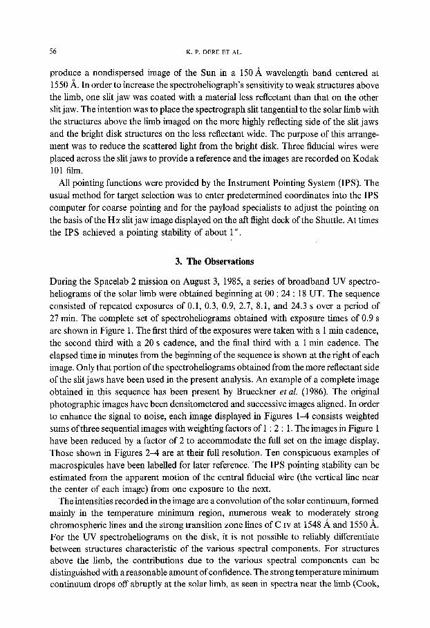
produce a nondispersed image of the Sun in a 150 .~ wavelength band centered at 1550 A. In order to increase the spectroheliograph's sensitivity to weak structures above the limb, one slit jaw was coated with a material less reflectant than that on the other slit jaw. The intention was to place the spectrograph slit tangential to the solar limb with the structures above the limb imaged on the more highly reflecting side of the slit jaws and the bright disk structures on the less reflectant wide. The purpose of this arrange- ment was to reduce the scattered light from the bright disk. Three fiducial wires were placed across the slit jaws to provide a reference and the images are recorded on Kodak 101 film.

All pointing functions were provided by the Instrument Pointing System (IPS). The usual method for target selection was to enter predetermined coordinates into the IPS computer for coarse pointing and for the payload specialists to adjust the pointing on the basis of the Ha slit jaw image displayed on the aft flight deck of the Shuttle. At times the IPS achieved a pointing stability of about 1"

3. The Observations

During the Spacelab 2 mission on August 3, 1985, a series of broadband UV spectroheliograms of the solar limb were obtained beginning at 00 : 24 : 18 UT. The sequence consisted of repeated exposures of 0.1, 0.3, 0.9, 2.7, 8.1, and 24.3 s over a period of 27 min. The complete set of spectroheliograms obtained with exposure times of 0.9 s are shown in Figure 1. The first third of the exposures were taken with a 1 min cadence, the second third with a 20 s cadence, and the final third with a 1 min cadence. The elapsed time in minutes from the beginning of the sequence is shown at the right of each image. Only that portion of the spectroheliograms obtained from the more reflectant side of the slit jaws have been used in the present analysis. An example of a complete image obtained in this sequence has been present by Brueckner et al. (1986). The original photographic images have been densitometered and successive images aligned. In order to enhance the signal to noise, each image displayed in Figures 1-4 consists weighted sums of three sequential images with weighting factors of 1 : 2 : 1. The images in Figure 1 have been reduced by a factor of 2 to accommodate the full set on the image display. Those shown in Figures 2-4 are at their full resolution. Ten conspicuous examples of macrospicules have been labelled for later reference. The IPS pointing stability can be estimated from the apparent motion of the central fiducial wire (the vertical line near the center of each image) from one exposure to the next.

The intensities recorded in the image are a convolution of the solar continuum, formed mainly in the temperature minimum region, numerous weak to moderately strong chromospheric lines and the strong transition zone lines of C Iv at 1548 A and 1550 ,~. For the UV spectroheliograms on the disk, it is not possible to reliably differentiate between structures characteristic of the various spectral components. For structures above the limb, the contributions due to the various spectral components can be distinguished with a reasonable amount of confidence. The strong temperature minimum continuum drops off abruptly at the solar limb, as seen in spectra near the limb (Cook,

OBSERVATIONS OF MACROSPICULES AT THE SOLAR LIMB 57

Fig. 1. The complete series of UV spectroheliograms of the solar limb obtained during one observing program during Spacelab 2. The time in minutes from the beginning of the sequence is marked at the right

in each image. Ten macrospicules are labelled for reference in the text.

Brueckner, and Bartoe, 1983). Many of the chromospheric lines also fall off as rapidly

but other chromospheric lines such as Fe II peak roughly 1000 km above the temperature minimum but some 2400 km below the C IV emission peak (Dere, Bartoe, and Brueckner, 1986a). Thus, structures seen in the spectroheliograph images within a few arc sec of the limb have both chromospheric and transition zone components but those

structures seen much higher are most likely to be due to the C IV transition zone emission at 105K.

For this observing sequence, the slit was placed at an angle such that the slit would

be tangent to the limb at a latitude of 63 ~ He H 10830 spectroheliograms published in Solar Geophysical Data show that the north polar coronal hole extended down to a latitude of 54 ~ on the west limb. The region displayed in Figure 1 include the latitudes from 51 ~ to 75 ~ north. Macrospicules are clearly evident in these spectroheliograms and their location is consistent with lying inside the boundaries of the northern polar coronal hole. The physical characteristics of the macrospicules observed in this data set have been measured and are presented and discussed in the following sections.

58 K.P . DERE ET AL.

Also of interest is the mound of emission seen just to the left of the central fiducial wire. It forms at around 12 min into the observing period and has faded by 25 min. The mound is characterized highly variable diffuse emission at altitude above the main bulk of emission which delineates the mound. These highly variable emissions may well be signatures of expulsions of plasma that are commonly seen as Doppler shifts in spectra of transition zone fines on the disk, where high velocity jets with velocities of up to 500 km s- ' and explosive events with velocities around 100 km s- 1 are found (Brueckner and Bartoe, 1983). An analysis of rastered C IV spectra has also shown expulsions of material from quiet network elements on the disk in both intensity and Doppler images (Dere, Bartoe, and Brueckner, 1986b). The behavior of this mound of emission leads us to tentatively identify it as a region of plasma expulsion but the images are not sufficiently distinct to make very definite conclusion concerning it.

Portions of the spectroheliograms outside of the field shown in Figures 1-3 also show evidence for the UV counterparts of the ubiquitous spicules commonly seen in Ha (Brueckner et aL, 1986). These confirm a similar result found by comparing Ha spectroheliograms and rastered UV slit spectra (Dere, Bartoe, and Brueckner, 1986a).

4. Properties of Maerospieules

Macrospicules were first discovered at extreme ultraviolet wavelengths by Bohlin et al.

(1975). Additional observations of two large macrospicules were reported by Withbroe et al. (1976). Both papers were based on observations made during the Skylab mission. Some time ago Waldmeier (1955) described He macrospicules at the solar poles but otherwise they provoked little scientific interest until the EUV data became available. LaBonte (1979) has summarized the properties of macrospicules observed in He.

The 10 macrospicules that have been labelled in Figure 1 provide a sample from which the average characteristics of macrospicules have been determined. It is possible that some of the macrospicules seen quite early are the same basic structure seen in the later images with the highest pointing stability but the deterioration in pointing stability at times centered around 7 min obscures this identification. For the purpose of this study, they are considered to be separate events.

4.1. LENGTH

The macrospicules range in length from 5 to 23" with an average length of 12", when measured above the average C IV limb. Bohlin et aL (1975) report typical lengths of a similar order but also report events as long as 30-60" and Withbroe et al. (1976) report 2 events of length 40-50". We have not observed any of these exceptionally large events.

4.2. WIDTH

The macrospicules show a range in width near their base of from 3 to 9" with an average of 6". These values are somewhat lower than those measured by Bohlin et al. (1975) but the difference is probably not significant.


4.3. SHAPE

Macrospicules generally fit the description of B ohlin et al. (1975) as being tapered linear

structures although an important exception can be pointed out. The large macrospicule (No. 10) seen in Figure 2 to the right of the central fiducial wire shows clear evidence

of a hook-like feature at its tip near the peak of its development.

Fig. 2. A selected time series of UV spectroheliograms. The time in minutes from the beginning of the sequence is marked to the right in each image.

4.4. ORIENTATION

Bohlin et al. concluded that macrospicules fan out away from the solar pole and, in general, the macrospicules shown in Figure 1 support this statement. But, again, there

is not a strict conformation to this rule and there are examples of nearly radial macrospicules in regions where most of the macrospicules are tilted, such as macrospicule No. 8 in Figure 3. There is also a good example of a macrospicule which shows a definite change in orientation during its lifetime, as discussed in the next section.

4.5 TEMPORAL DEVELOPMENT AND LIFETIME

Figures 2 and 3 show the evolution of 3 macrospicules. Figure 2 shows the growth phase of a large macrospieule (No. 10) to the right of the central fiducial wire. First signs of

60 K. P. DERE ET AL.

Fig. 3. A selected time series of UV spectroheliograms. The time in minutes from the beginning of the sequence is marked to the right in each image.

this macrospicule appear at around 10 min into the observing period but it does not enter

the strongest period of growth until about 14 min when it begins a clear rise. The

apparent outward velocity is about 20 km s - 1. At maximum phase, a distinct hook is

seen at its tip. By 27 min, it has almost completely faded. The macrospicule can be seen

from roughly 10 to 27 min but the duration of the main event is about 10 min.

Figure 3 shows a rapidly evolving macrospicule (No. 8) to the left of the central fiducial wire on 3 consecutive exposures at elapsed times of 22 to 24 min. The lifetime of this event is then about 3 min and is the shortest lived event observed. The apparent outward velocity is about 45 km s - 1

Another outstanding example of a macrospicule (No. 9) is seen in this same figure.

The apparent outward velocity in the rise phase of this macrospicule is about 30 km s 1. This example also exhibite a small but visible change in orientation. At 19 min it makes an angle of about 30 ~ to the vertical in Figure 2 and at 20 min, it has moved to an angle of 35 ~ By 22 min it is at an angle of 40 ~ to the vertical where it remains for the rest of its lifetime.


The rise phase of the two largest macrospicules (No. 9 and No. 10) shown in Figures 2

and 3 exhibit a fairly steady extension of emission to higher altitudes. When these

macrospicules reach maximum height, there are small but significant variations in the

maximum height with time. The decay phase cannot be described as simply the reverse

of the rise phase with emission moving to lower altitudes but more as a fading in place

and a subsequent disappearance. There are some indications, at the limit of our ability

to determine such things, that the macrospicules breaks up into knots or condensations

during its decay.

4.6. SUMMARY

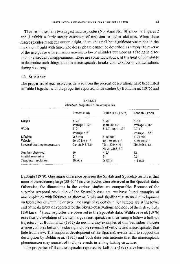
The properties of macrospicules derived from the present observations have been listed

in Table I together with the properties reported in the studies by Bohlin e t al. (1975) and

TABLE I Observed properties of macrospicules

Present study Bohlin et al. (1975) Labonte (1979)

Length 5-23" 8-25" 8-33" average = 12" some 30-60" average = 16"

Width 3-9" 5-15", up to 30" 0.7-6" average = 6" average = 2.5"

Lifetime > 3 min 8--45 min 4-24 min Velocity 20-50 km s ~ 10-150 km s - 1 <60 km s- Spectral line/Log temperature C IV 21548 / 5.0 He II 2304 / 4.9 He 26562 / 4.0

NevrI 2465/5.7 Number observed 10 ~ 25 32 Spatial resolution 2" 2" 0.5" Temporal resolution 20, 60 s > 180 s ~ 1 min

LaBonte (1979). One major difference between the Skylab and Spacelab results is that

none of the extremely large (30-60") macrospicules were observed in the Spacelab data.

Otherwise, the dimensions in the various studies are comparable. Because of the

superior temporal resolution of the Spacelab data set, we have found examples of

macrospicules with lifetimes as short as 3 min and significant structural development

on timescales of a minute or two. The range of velocities in our sample are at the lower

end of the distribution reported for the Skylab observations and none of the high velocity

(150 km s - i) macrospicules are observed in the Spacelab data. Withbroe et al. (1976)

note that the evolution of the two large macrospicules in their sample follow a ballistic trajectory but Bohlin e t al. (1975) do not find any examples of this but rather indicate a more complex behavior inducing multiple reversals of velocity and macrospicules that fade from view. The temporal development of the Spacelab events tend to support the description by Bohlin e t al. (1975) and both data sets indicate that the macrospicule phenomenon may consist of multiple events in a long lasting structure.

The properties of H a macrospicules reported by LaBorite (1979) have been included

62 K . P . DERE ET AL.

in Table I for the sake of completeness. It is not clear that LaBonte's He observations refer to the same structures as the UV observations. For instance, the UV macrospicules

are limited to the polar coronal holes but LaBonte reports He macrospicules at all

latitudes whereas Waldmeier found the He macrospicules limited to the polar regions.

The difference may be traced to LaBonte's inclusion of a wider range of phenomena,

such as filament eruptions, under the category of macrospicule.

In Figure 4 we present an image obtained by summing the exposures at 21, 22, 23,

and 24 min in order to display a composite of the 3 strongest macrospicules at a somewhat higher signal-to-noise ratio.

Fig. 4. Summed UV spectroheliograms.

5. Discussion

The present set of observations have added to our understanding of the characteristics of macrospicules, in particular, their short-term evolution. Because they exhibit a rather definite outward motion and a subsequent decay rather than a collapse back to the solar surface, they are candidates for sources of mass outflow into the solar wind which is strongly influenced by the open field regions in polar coronal holes where the macrospicules are formed. Reliable estimates of the mass flux involved in the macrospicules


must await a determination of their fill factor and of their birthrate which is hard to determine from limb data where all EUV macrospicules have been observed. Various identifications of macrospicules with other structures on the disk have been suggested. Because all of these are based on observations at the limb where the large line of sight makes it extremely difficult to demonstrate the relationship of one structure to another, these identifications must still be considered tentative.

References

Bohlin, J. D., Vogel, S. N., Purcell, J. D., Sheeley, N. R., Tousey, R., and Van Hoosier, M. E.: 1975, Astrophys. J. 197, L133.

Brueckner, G. E. and Bartoe, J.-D. F.: 1983, Astrophys. J. 272, 329. Brueckner, G. E., Bartoe, J.-D. F., Cook, J. W., Dere, K. P., and Socker, D. G.: 1986, Adv. Space Sci. 6,

263. Cook, J. W., Brueckner, G. E., and Bartoe, J.-D. F.: 1983, Astrophys. J. 270, L89. Dere, K. P., Bartoe, J.-D. F., and Brueckner, G. E.: 1986a, Astrophys. J. 305, 947. Dere, K. P., Bartoe, J.-D. F., and Brueckner, G. E.: 1986b, Astrophys. J. 310, 456. LaBonte, B. J.: 1979, Solar Phys. 61,283. Waldmeier, M.: 1955, Ergebnisse und Probleme der Sonnenforschung, Akademische Verlagsgesellschaft,

Leipzig. Withbroe, G. L., Jaffee, D. T., Foukal, P. V., Huber, M. C. E., Noyes, R. W., Reeves, E. M., Schmahl, E.

J., Timothy, J. G., and Vernazza, J. E.: 1976, Astrophys. J. 203, 528.

uv observations of macrospicules at the solar limb

Documents