1

Using three statistical methods to analyze the 1

association between exposure to 9 compounds and 2

obesity in children and adolescents: National Health 3

and Nutrition Examination Survey 20052010 4

Bangsheng Wu1,2, Yi Jiang1,2, Xiaoqing Jin1,*, Li He3,* 5

1 Emergency Department, Zhongnan Hospital of Wuhan University, 169 Donghu 6

Road, Wuhan 430071, Hubei, China 7

2 Second Clinical School, Wuhan University, Wuhan 430071, Hubei, China 8

3 Internal hematology, Zhongnan Hospital of Wuhan University, 169 Donghu Road, 9

Wuhan 430071, Hubei, China 10

* Correspondence information: redjin@whu.edu.cn (Xiaoqing Jin), Tel: 11

+8618062765135; lihe126@hotmail.com (Li He), Tel: 15377550399 12

Authors: Bangsheng Wu, 2016302180323@whu.edu.cn; Yi Jiang, 13

1059688932@qq.com 14

Abstract 15

Background: Various risk factors influence obesity differently, and 16

environmental endocrine disruption may increase the occurrence of obesity. 17

However, most of the previous studies have considered only a unitary 18

exposure or a set of similar exposures instead of mixed exposures, which 19

2

entail complicated interactions. We utilized three statistical models to 20

evaluate the correlations between mixed chemicals to analyze the 21

association between 9 different chemical exposures and obesity in 22

children and adolescents. 23

Methods: We fitted the generalized linear regression, weighted quantile 24

sum (WQS) regression, and Bayesian kernel machine regression (BKMR) 25

to analyze the association between the mixed exposures and obesity in the 26

participants aged 619 in the National Health and Nutrition Examination 27

Survey (NHANES) 2005–2010. 28

Results: In the multivariable logistic regression model, 29

2,5-dichlorophenol (2,5-DCP) (OR (95% CI): 1.25 (1.11, 1.40)), monoethyl 30

phthalate (MEP) (OR (95% CI): 1.28 (1.04, 1.58)), and mono-isobutyl 31

phthalate (MiBP) (OR (95% CI): 1.42 (1.07, 1.89)) were found to be 32

positively associated with obesity, while methylparaben (MeP) (OR (95% 33

CI): 0.80 (0.68, 0.94)) was negatively associated with obesity. In the 34

multivariable linear regression, MEP was found to be positively 35

associated with the body mass index (BMI) z-score (𝛽 (95% CI): 0.12 (0.02, 36

0.21)). In the WQS regression model, the WQS index had a significant 37

association (OR (95% CI): 1.48 (1.16, 1.89)) with the outcome in the obesity 38

model, in which 2,5-DCP (weighted 0.41), bisphenol A (BPA) (weighted 39

0.17) and MEP (weighted 0.14) all had relatively high weights. In the 40

3

BKMR model, despite no statistically significant difference in the overall 41

association between the chemical mixtures and the outcome (obesity or 42

BMI z-score), there was nonetheless an increasing trend. 2,5-DCP and 43

MEP were found to be positively associated with the outcome (obesity or 44

BMI z-score), while fixing other chemicals at their median 45

concentrations. 46

Conclusion: Comparing the three statistical models, we found that 47

2,5-DCP and MEP may play an important role in obesity. Considering the 48

advantages and disadvantages of the three statistical models, our study 49

confirms the necessity to combine different statistical models on obesity 50

when dealing with mixed exposures. 51

Keywords: obesity; adolescent; child; weighted quantile sum (WQS) 52

regression; Bayesian kernel machine regression (BKMR) 53

Introduction 54

The continuous increase in obesity has become an important worldwide health 55

problem in the past 30 years [1]. In 2016, about 18% of children and adolescents aged 56

519 were overweight or obese [2]. Obesity in children increases the risk of health 57

conditions, such as coronary heart disease, diabetes mellitus, hypertension, and heart 58

failure, and those obese children or adolescents can become obese adults [3-5]. 59

Therefore, it is vital to identify potential risk factors contributing to obesity to reduce 60

the prevalence and mortality rates in obesity-related diseases. Although genetic 61

4

predisposition, physical activity, and diet play an essential role in the occurrence of 62

obesity, there is still a need for further explanation. More evidence indicates that 63

environmental endocrine-disrupting chemicals might increase the occurrence of 64

obesity [6-9]. Twum et al. demonstrated an underlying relation between exposure to 65

2,5-dichlorophenol (2,5-DCP) and obesity in children [4]. A significant association 66

was found between bisphenol A (BPA) and general and abdominal obesity [10]. 67

Deierlein showed that phthalates—specifically low-molecular weight phthalates 68

(monoethyl phthalate [MEP], a metabolite of diethyl phthalate (DEP); mono-n-butyl 69

phthalate [MBP], a metabolite of di-n-butyl phthalate (DBP), and mono-isobutyl 70

phthalate [MiBP], a metabolite of di-isobutyl phthalate (DiBP))—had slight 71

associations with girls' anthropometric outcomes [11]. These substances are readily 72

present in our daily lives, since consumer products usually use parabens as 73

preservatives, building and food packaging materials use phthalates as plasticizers, 74

and the production of pharmaceutical and agricultural products uses 2,5-DCP as a 75

chemical intermediate [12-14]. We can easily contact these environmental 76

endocrine-disrupting chemicals via gastrointestinal intake, dermal contact, and 77

applying products that contain these chemicals [15, 16]. However, most of the 78

previous research studied only a unitary exposure or a set of similar exposures [17-19]. 79

We are exposed to all kinds of chemical exposures simultaneously, which can result in 80

complicated interactions. Therefore, it is necessary to use a suitable statistical model 81

for risk assessment of exposure and obesity [20-22]. 82

5

We collected data on urinary chemicals or metabolites that had been reported to 83

have an effect on obesity in the National Health and Nutrition Examination Survey 84

(NHANES) from 2005 to 2010. We studied 9 chemical exposures including phenols 85

(BPA, benzophenone-3 (BP-3)), parabens (methylparaben (MeP), propyl paraben 86

(PrP)), pesticides (2,5-DCP, 2,4-DCP) and phthalate metabolites (Mono-benzyl 87

phthalate (MBzP), MEP, MiBP). We selected three statistical methods, including 88

generalized linear regression, weighted quantile sum (WQS) regression, and Bayesian 89

kernel machine regression (BKMR) models, to better analyze multi-exposures’ 90

co-function on adolescent obesity. Among them, BKMR model can resolve the 91

non-linear and complicated interactions between chemical exposures and get more 92

accurate results comparing with the generalized linear regression[23]. All of these 93

three methods have their own advantages and disadvantages, and we expected that 94

this comprehensive analysis would yield insightful and fruitful conclusions. 95

Methods 96

Study sample 97

The NHANES is a cross-sectional nationally representative program, aiming to 98

collect information on adults’ and children’s health and nutritional condition in the 99

United States, which is reviewed and approved by the National Center for Health 100

Statistics, as one of the departments of Centers for Disease Control and Prevention 101

(CDC). The NHANES program was conducted in the early 1960s and released the 102

data in biennial datasets. In order to get the unbiased national health information on 103

6

the non-institutionalized population of the United States, the NHANES used a 104

considerate, multi-stage stratification probability sampling design[24]. We collected 105

publicly accessible data from 2005 and 2010. We selected participants between 6 and 106

19 years old, with attainable measurements of urinary phenols, parabens, pesticides, 107

and phthalate metabolites Body mass index (BMI) and waistcircumference 108

simultaneously (n=2629) and excluded the participants whose data on covariates, 109

including age, gender, race, education level, family income-to-poverty ratio, caloric 110

intake, serum cotinine, and urinary creatinine, were missing (n=257). Finally, 2372 111

participants were included in our study. 112

Measurement of chemical exposures 113

Urinary samples were collected and stored at -20°C. They were sent to the National 114

Center for Environmental Health, the Organic Analytical Toxicology Branch, for 115

analysis. BPA, BP-3, MeP, PrP, 2,4-DCP, and 2,5-DCP,were extracted by on-line 116

solid-phase extraction (SPE). They were measured by high-performance liquid 117

chromatography as well as tandem mass spectrometry (MS/MS). MBzP, MEP, and 118

MiBP were measured by high-performance liquid chromatography-electrospray 119

ionization-tandem mass spectrometry (HPLC-ESI-MS/MS). The limit of detection 120

(LOD) for the compounds to be analyzed, including BPA, BP-3, MeP, PrP, 2,4-DCP, 121

and 2,5-DCP, were 0.4 ng/mL, 0.4 ng/mL, 1.0 ng/mL, 0.2 ng/mL, 0.2 ng/mL, 0.2 122

ng/mL in the data from 2005 to 2010, respectively. And the LOD for MBzP, MEP, and 123

MiBP were 0.3 ng/mL, 0.8 ng/mL, and 0.3 ng/mL in the data from 2005 to 2008 and 124

7

0.2 ng/mL, 0.4 ng/mL, and 0.2 ng/mL in the data from 2009 to 2010. These values 125

below the limit of detection were divided by the square root of 2 to replace the 126

original values. As one study recommended [25], we treated urinary creatinine as a 127

covariate to explain the urinary dilution. Urinary creatinine was measured by a 128

Beckman Synchron CX3 Clinical Analyzer. The NHANES provides detailed 129

information on the measurement method in the section on laboratory methods on its 130

website [26, 27]. 131

Anthropometric variables 132

Trained health technicians measured the body weight and height according to the 133

standardized protocol. The BMI was calculated using each person’s weight in 134

kilograms to divide the square of their height in meters. However, because the 135

standard BMI shows differences for the different ages and gender among children, 136

measuring BMI percentiles and the BMI z-score was more appropriate. The BMI 137

z-score was calculated in regards to the children’s age, gender, and BMI. An 138

appropriate standard was used, which reflected the number of SDs differing from the 139

mean of the BMI with reference to the same age and gender. The methodology to 140

calculate the BMI z-score specifically for different ages and gender was provided by 141

the CDC [28]. We defined a child to be obese when their BMI was above or equal to 142

the 95th percentile for their age and gender in accordance with the CDC 143

recommendations [29]. 144

8

Covariates 145

Covariates, including age, gender, race, education level, family income-to-poverty 146

ratio, caloric intake, serum cotinine, and urinary creatinine, were collected by 147

interview or laboratory detection by NHANES. Race was grouped into Mexican 148

American, Other Hispanic, Non-Hispanic White, Non-Hispanic Black, and Other 149

Race. Education level was categorically grouped into ≤5 grade, 6−8 grade, 9−12 150

grade, or High School Graduate with No Diploma, High School Graduate and GED or 151

Equivalent, or More than high school. The family income-to-poverty ratio was 152

divided into three groups: ≤1.30, 1.31−3.50, and >3.50. The caloric intake was 153

dichotomously divided into normal intake and excessive intake, according to the 154

Dietary Guidelines for Americans 2010 [30]. Serum cotinine indirectly reflected the 155

exposure to environmental tobacco. Serum cotinine, age, and urinary creatinine were 156

considered to be continuous variables. 157

Statistical analysis 158

We used the χ2 test and the t-test to analyze categorical variables and continuous 159

variables, respectively. And for the serum cotinine and urinary creatinine, we used 160

wilcoxon rank-sum test. We calculated the descriptive statistics on BPA, BP-3, MeP, 161

PrP, 2,4-DCP, 2,5-DCP, MBzP, MEP, and MiBP. Because the distributions of the 162

chemical exposures were skewed, we log-transformed the concentrations of all 163

chemical exposures. We used the Pearson correlation to calculate the correlation 164

9

coefficients among all chemical exposures. p < 0.05 was considered to be statistically 165

significant. 166

Generalized linear regression 167

We conducted multivariable logistic regression to analyze each chemical exposure 168

and the odds ratios (ORs) of obesity in different quartiles. We also fitted a 169

multivariable linear regression model to assess the association between each chemical 170

exposure and the continuous variable of the BMI z-score in different quantiles. In 171

addition, we fitted the models, adjusting for all the chemical exposures. All the 172

regression models were adjusted by age, gender, race, education level, family 173

income-to-poverty ratio, caloric intake, serum cotinine, and urinary creatinine. We 174

used log-transformed urinary creatinine as an independent covariate instead of the 175

creatinine-adjusted concentration [25]. 176

Weighted quantile sum (WQS) regression 177

The WQS model scored all the chemical exposures into quantiles and estimated the 178

weight index: 179

ℊ(𝜇) = 𝛽0 + 𝛽1 (∑ 𝜔𝑖

𝑐

𝑖=1

𝑞𝑖) + 𝑧′𝜑, 180

where ℊ() represents any monotonic link function, μ is the predictable variable, 𝜔 181

is the weight of the ith components to be estimated, qi refers to different quantiles, 182

and (∑ 𝜔𝑖𝑐𝑖=1 𝑞𝑖) represents the weight quantile sum of the set of c components of 183

10

interest. Furthermore, 𝛽1 denotes the regression coefficient for the weight quantile 184

sum, 𝛽0 is the intercept, 𝑧′ refers to the covariates, including risk factors and 185

confounders, and 𝜑 is the coefficients for the covariates. The weights were estimated 186

between 0 and 1, and added up to 1. In this study, we divided the data into the training 187

set (40%) and the validation set (60%), we also set 𝛽1 to be positive and the seed 188

was set to be 2019. Besides, we also constrained 𝛽1 to be negative to find if there 189

was a significant relationship in this way. We bootstrapped the training set 10000 190

times and got the estimated weights, which maximized the likelihood of the 191

non-linear model. A significant level (p < 0.05) was set to test the significance of the 192

weights in each bootstrap. We calculated the �̅�𝑖 to estimate the weight quantile sum: 193

WQS = ∑ �̅�𝑖𝑞𝑖

𝑐

𝑖=1

194

�̅�𝑖 = (1 𝑛𝐵⁄ ) ∑ 𝜔𝑖𝑗,

𝑛𝐵

𝑗=1

195

where 𝑛𝐵 represents the number of bootstraps in which 𝛽1 was significant. The 196

estimated WQS was then determined using the validation set. All the chemical 197

exposures were included in the model, and a specific weight was calculated for each 198

component, representing their contribution to the WQS index. The chemical 199

exposures included were constrained to have the same effect with the outcome (all 200

positive or all negative).[31] 201

11

Bayesian kernel machine regression (BKMR) 202

The BKMR model utilizes a non-parametric approach to flexibly model the 203

association between chemical exposures and healthy outcomes, including the 204

nonlinear and/or interactions in the exposure-outcome association. A high-dimension 205

exposure-response relationship induced by multiple variables incorporated in the 206

model would make it difficult to ascertain the basis function. Thus, we used a kernel 207

machine regression: 208

𝑌𝑖 = ℎ(𝑧𝑖) + 𝑥𝑖𝛽 + 𝜖𝑖 , 209

where 𝑌𝑖 is the health outcome, i refers to the individual (i = 1, 2, 3…n), 𝑧𝑖 is the 210

chemical exposures, 𝑥𝑖 is the potential confounders, and 𝛽 represents the effect of 211

the covariates. 𝜖𝑖 is the residual that obeys the normal distribution N (0, 𝜎2). ℎ() is 212

the function that fits the exposure and the outcome considering nonlinear and 213

interactions between the exposures. We grouped the chemical exposures into three 214

groups (group1: BPA, BP-3, MeP, and PrP; group2: 2,5-DCP and 2,4-DCP; group3: 215

MBzP, MEP, and MiBP), according to their source and correlation (chemical 216

exposures with high correlation were grouped) with each other. A hierarchical 217

variable selection approach was used to estimate the posterior inclusion probability of 218

highly correlated variables, which was based on our prior knowledge. The model was 219

fit with 10000 iterations using a Markov chain Monte Carlo (MCMC) method. The 220

parameter r.jump2 was separately set to 0.2 (in the BMI z-score model) and 0.001 (in 221

the obesity model) to get suitable acceptance rates. 222

12

We also analyzed the association between the quantiles of the chemical exposures 223

and binary healthy outcome (obesity and non-obesity) using a probit BKMR model: 224

Φ−1(𝜇𝑖) = ℎ(𝑧𝑖) + 𝑥𝑖𝛽, 225

where Φ−1 is the link function and 𝜇𝑖 is the probability of the binary outcome.[22, 226

23] 227

Trace plots of parameter in both BMI z-score and obesity model were visualized to 228

investigate the convergence. 229

All of the statistical analysis were conducted using R software (version 3.6.0). 230

Results 231

There were 2372 children and adolescents included in our study. The general 232

characteristics of the participants are presented in Table 1. The prevalence of obesity 233

was 20.53%. It showed that the mean age of obesity and non-obesity is close: 234

approximately 12-and-a-half years old. About half (44.98%) of the participants were 235

≤5 grade, and 53.03% had a normal caloric intake. The mean (SD) BMI and waist 236

237

Table 1 Demographic characteristics of the NHANES 2005–2010 participants (N = 238

2372), aged 619 years 239

Characteristics Obesity

487 (20.53%)

No obesity

1885 (79.47%)

P value

Age (y), mean (SD) 12.57 (3.81) 12.51 (4.01) 0.729

13

Gender 0.931

Male 252 (10.62%) 982 (41.40%)

Female 235 (9.91%) 903 (38.07%)

Race <0.001

Mexican American 143 (6.03%) 516 (21.75%)

Other Hispanic 52 (2.19%) 152 (6.41%)

Non-Hispanic White 112 (4.72%) 615 (25.93%)

Non-Hispanic Black 157 (6.62%) 491 (20.70%)

Other Race 23 (0.97%) 111 (4.68%)

Education level 0.155

5 grade 215 (9.06%) 852 (35.92%)

6-8 grade 118 (4.97%) 409 (17.24%)

9-12 grade, No Diploma 115 (4.85%) 453 (19.10%)

High School Graduate 26 (1.10%) 79 (3.33%)

GED or Equivalent, More than high

school

13 (0.55%) 92 (3.88%)

Family income-to-poverty ratio 0.003

1.30 235 (9.91%) 774 (32.63%)

1.31,3.50 177 (7.46%) 706 (29.76%)

>3.50 75 (3.16%) 405 (17.07%)

Caloric intake 0.014

Normal intake 283 (11.93%) 975 (41.10%)

Excessive intake 204 (8.60%) 910 (38.36%)

Serum cotinine (ng/mL), GM (SD) 0.13 (10.55) 0.13 (14.48) 0.140*

Urinary creatinine (mg/dL), GM (SD) 119.89 (1.88) 107.53 (2.01) 0.005*

BMI, mean (SD) 30.41 (6.99) 19.68 (3.66) <0.001

BMI z-score, mean (SD) 2.12 (0.32) 0.18 (0.94) <0.001

14

Waist Circumference (cm), mean (SD) 96.17 (18.05) 69.79 (11.36) <0.001

NHANES: National Health and Nutrition Examination Survey; BMI: body mass 240

index. Data are presented as mean ± SD or Geometric mean ± SD or n (%). The 241

t-test and 𝜒2 test were between the general obesity and no obesity groups. 242

*Wilcoxon rank-sum test was used for the non-normal distribution data. 243

244

circumferences were 30.41 (6.99) and 96.17 (18.05) cm in the obesity group and 245

19.68 (3.66) and 69.79 (11.36) cm in the non-obesity group, respectively. The mean 246

(SD) BMI z-scores were 2.12 (0.32) in the obesity group and 0.18 (0.94) in the 247

non-obesity group. There were significant differences between the obesity and 248

non-obesity participants in terms of race, family income, caloric intake, urinary 249

creatinine, BMI, BMI z-score, and waist circumference. 250

The LOD and the detection frequency of the chemicals above the LOD are shown 251

in Table 2. The detection frequency of MEP (99.9%) had the highest detection 252

frequency of chemical exposures and the detection frequency of all chemical 253

exposures was above 90%. Table 2 also shows the geometric mean, the mean, and the 254

distribution of the chemical exposures. The highest and the lowest geometric means 255

of the chemical exposures were related to the MEP (87.12) ng/mL and 2,4,5-TCP 256

(0.09) μg ∕ L. 257

We found significant correlations (P < 0.05) among 9 chemicals (Fig. 1), except for 258

the correlation between BP-3 and 2,4-DCP (P = 0.69). There was a positive 259

15

correlation between other compounds, except for a nearly no correlation of BP-3 with 260

2,5-DCP (r = -0.06). 2,5-DCP was found to have a strongly correlation with 2,4-DCP 261

(r = 0.87). Additionally, a high correlation between MeP and PrP (r = 0.81) was 262

found. 263

The results from the multivariable logistic and linear regression models adjusted for 264

the covariates are shown in Tables 3 and 4, respectively. The adjusted multivariable 265

logistic regression analysis revealed a statistically significant association between 266

obesity and MeP (OR (95% CI): 0.80 (0.68, 0.94)), 2,5-DCP (OR (95% CI): 1.25 267

(1.11, 1.40)), MEP (OR (95% CI): 1.28 (1.04, 1.58)), and MiBP (OR (95% CI): 1.42 268

(1.07, 1.89)), with MeP showing a negative association with dichotomous variable 269

obesity. PrP was found to have a negative association with obesity only when 270

comparing the 4th quartile with the reference quartile (OR (95% CI): 0.69 (0.49, 271

0.98)). When comparing the 2nd, 3rd, and 4th 2,5-DCP quartiles with the reference 272

quartile, 2,5-DCP had a higher odds ratio (OR (95% CI): 1.49 (1.07, 2.07); 1.80 (1.30, 273

2.51), and 2.06 (1.47, 2.89), respectively) (Table 3). When comparing the second, 274

third, and fourth quartiles of MEP with the reference quartile, MEP had a higher odds 275

ratio (OR (95% CI): 1.04 (0.75, 1.43); 1.28 (0.92, 1.79), and 1.39 (0.98, 1.98), 276

respectively; Table 3). We used adjusted multivariable linear regression to evaluate 277

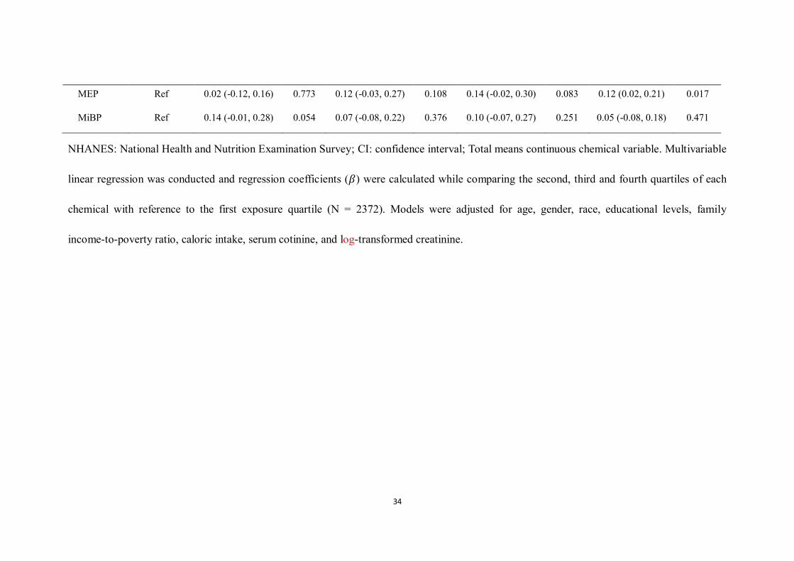
the relation between 9 chemical exposures and the BMI z-score (Table 4). We found 278

MeP (second vs. first quartile) to be negatively associated with the BMI z-score (𝛽 279

(95% CI): -0.14 (-0.27, -0.01)), and 2,5-DCP (third vs. first quartile) as well as MEP 280

16

to be positively associated with the BMI z-score (𝛽 (95% CI): 0.16 (0.02, 0.30); 0.12 281

(0.02, 0.21), respectively). The second, third, and fourth MEP quartiles had a higher 282

BMI z-score (𝛽 (95% CI): 0.02 (-0.12, 0.16); 0.12 (-0.03, 0.27), and 0.14 (-0.02, 283

0.30), respectively) compared with the lowest reference quartile (Table 4). 284

In the multivariable logistic and linear regression models, including all the 285

chemical exposures, adjusting for the confounding effects of other chemicals, 286

2,5-DCP, 2,4-DCP, and MEP were found to have a significant association with both 287

the dichotomous variable obesity (OR (95% CI): 1.73 (1.35, 2.24), 0.57 (0.40, 0.82), 288

and 1.35 (1.08, 1.69), respectively) and continuous variate BMI z-score (𝛽 (95% CI): 289

0.14 (0.04, 0.24), -0.20 (-0.36, -0.05), and 0.15 (0.05, 0.25), respectively) (see 290

Additional File 1, Tables S1 and S2). We calculated the variance inflation factors 291

(VIFs) (see Additional File 1, Tables S3), and none of them was higher than 10. 292

293

Table 5 Association between the WQS index and obesity in NHANES 2005–2010 294

(N = 2372) 295

Outcomes OR/𝛽 95% CI of OR P value

Obesity

Model 1 1.50 (1.19, 1.90) <0.001

Model 2 1.51 (1.19, 1.91) <0.001

Model 3 1.48 (1.16, 1.89) 0.002

BMI z-score

Model 1 0.028 (-0.09, 0.15) 0.643

17

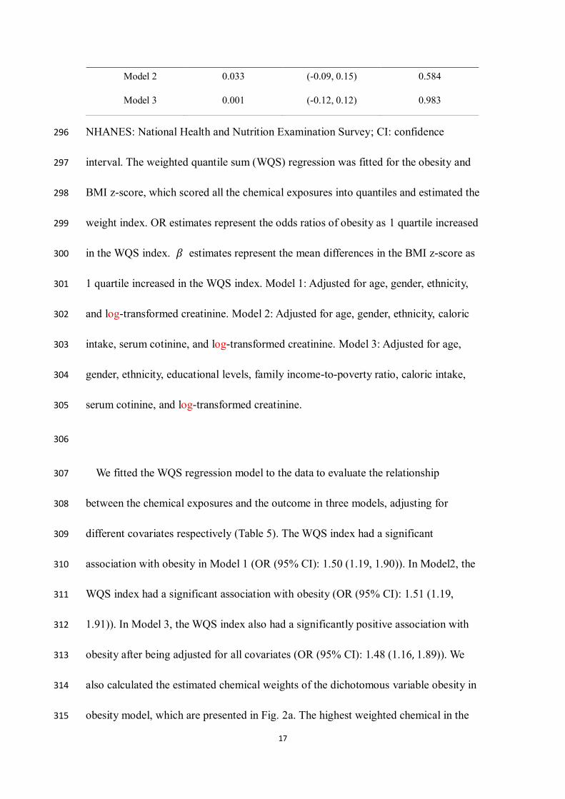
NHANES: National Health and Nutrition Examination Survey; CI: confidence 296

interval. The weighted quantile sum (WQS) regression was fitted for the obesity and 297

BMI z-score, which scored all the chemical exposures into quantiles and estimated the 298

weight index. OR estimates represent the odds ratios of obesity as 1 quartile increased 299

in the WQS index. 𝛽 estimates represent the mean differences in the BMI z-score as 300

1 quartile increased in the WQS index. Model 1: Adjusted for age, gender, ethnicity, 301

and log-transformed creatinine. Model 2: Adjusted for age, gender, ethnicity, caloric 302

intake, serum cotinine, and log-transformed creatinine. Model 3: Adjusted for age, 303

gender, ethnicity, educational levels, family income-to-poverty ratio, caloric intake, 304

serum cotinine, and log-transformed creatinine. 305

306

We fitted the WQS regression model to the data to evaluate the relationship 307

between the chemical exposures and the outcome in three models, adjusting for 308

different covariates respectively (Table 5). The WQS index had a significant 309

association with obesity in Model 1 (OR (95% CI): 1.50 (1.19, 1.90)). In Model2, the 310

WQS index had a significant association with obesity (OR (95% CI): 1.51 (1.19, 311

1.91)). In Model 3, the WQS index also had a significantly positive association with 312

obesity after being adjusted for all covariates (OR (95% CI): 1.48 (1.16, 1.89)). We 313

also calculated the estimated chemical weights of the dichotomous variable obesity in 314

obesity model, which are presented in Fig. 2a. The highest weighted chemical in the 315

Model 2 0.033 (-0.09, 0.15) 0.584

Model 3 0.001 (-0.12, 0.12) 0.983

18

fully adjusted obesity model was 2,5-DCP (weighted 0.41), followed by BPA and 316

MEP (weighted 0.17 and 0.16, respectively). We also treated the BMI z-score as a 317

continuous variable and fitted the BMI z-score model (Table 5). However, we did not 318

find any significant association between the exposures and the BMI z-score in all 319

three models. The estimated chemical weights of BMI z-score are presented in Fig. 2b. 320

The highest weighted chemical in the BMI z-score model was 2,5-DCP (weighted 321

0.30). Next to this were BP-3 and MEP, weighted 0.28 and 0.18, respectively. In 322

addition, we also fitted WQS model including all covariates with 𝛽1 constrained to 323

be negative. However, no statistical difference was found in this way. (see Additional 324

File 1, Tables S4) 325

326

Table 6 GroupPIP and condPIP in BKMR model in NHANES 2005–2010 (N = 327

2372) 328

Chemicals Group Obesity BMI z-score

groupPIP condPIP groupPIP condPIP

Phenols

BPA 1 0.775 0.020 0.329 0.278

BP-3 1 0.775 0.046 0.329 0.233

Paraben

MeP 1 0.775 0.903 0.329 0.322

PrP 1 0.775 0.031 0.329 0.166

Pesticides

2,5-DCP 2 0.966 0.978 0.256 0.500

19

GroupPIP: group posterior inclusion probability; condPIP: conditional posterior 329

inclusion probability; NHANES: National Health and Nutrition Examination Survey. 330

The three groups in BKMR model were Phenols and paraben (group1), pesticides 331

(group2), and phthalate metabolites (group3). Models were adjusted for age, gender, 332

race, educational levels, family income-to-poverty ratio, caloric intake, serum cotinine, 333

and log-transformed creatinine. 334

335

We grouped 9 chemical exposures into three groups, according to their source and 336

correlation with each other, and fitted the BKMR model to analyze the simultaneous 337

exposure with obesity and BMI z-score. In the obesity model, the group posterior 338

inclusion probabilities (PIP) of the pesticides group was 0.966, while the group PIP of 339

phenol and phthalates metabolites was higher than 0.5 (Table 6). In the pesticides 340

group, 2,5-DCP seemed to drive the effect of the whole group (CondPIP = 0.978; 341

Table 6). In the phthalate metabolites group, MEP drove the main effect of the whole 342

group (CondPIP: 0.656), while MeP drove the main effect in the phenols group 343

(CondPIP = 0.903) (Table 6). The overall association between the chemical mixtures 344

and the binomial outcome is shown in Fig. 3a. We found a positive tendency between 345

2,4-DCP 2 0.966 0.022 0.256 0.500

Phthalate

metabolites

MBzP 3 0.769 0.016 0.707 0.066

MEP 3 0.769 0.656 0.707 0.831

MiBP 3 0.769 0.328 0.707 0.103

20

chemical exposures and the outcome, in spite of no statistically significant difference. 346

Fig. 4 a illustrates the positive associations of 2,5-DCP, MEP, and MiBP with obesity 347

in the BKMR models, while controlling all other chemical exposures at their median 348

level. MeP demonstrated an inverse association with obesity, while no other chemical 349

exposures showed a noteworthy change in slope. We also investigated the relationship 350

between the outcome and a unitary predictor in exposures while fixing another 351

predictor in exposures at the 10th, 50th, and 90th quantiles (and holding the remnant 352

predictors to their median level), and the results are shown in Fig. 5 a. Since the 353

slopes were different between 2,5-DCP and obesity, MEP and obesity while fixing 354

MeP at the 10th, 50th, and 90th quantiles, potential interactions might exist between 355

2,5-DCP and MeP as well as MEP and MeP. In the BMI z-score model, the values of 356

the group PIP in three groups were 0.329, 0.256, and 0.707, respectively. (Table 6). 357

MEP drove the main effect in its group (CondPIP: 0.831). The overall risk of the 358

chemical mixtures on the outcome are presented in Fig. 3b. Although no statistically 359

significant difference was found, they revealed a positive association of the mixed 360

exposures with the BMI z-score, when we compared all the predictors fixed at 361

different levels with their 50th percentiles. 2,5-DCP and MEP had a trend of a 362

positive association with the BMI z-score, while 2,4-DCP had an inverse association 363

(Fig. 4 b). No obvious interaction was found in the BMI z-score model (Fig. 5 b). 364

21

To ensure the convergence, we plotted the trace plots, which showed a more or less 365

homogeneously covered space and indicated our model had a good convergence. (see 366

Additional File 1, Fig. 1 and Fig. 2) 367

For 2,5-DCP and MEP seemed to drive the whole effect in pesticides group (in 368

obesity model) and in phthalate group (in BMI z-score model), we further modeled 369

2,5-DCP and other groups (phenols group, parabens group, and phthalate group) in 370

obesity model and MEP and other groups (phenols group, parabens group, and 371

pesticides group) in BMI z-score model. The credibility intervals tighten a little (see 372

Additional File 1, Fig. 3 a and b), which meant 2,4-DCP, MiBP and MBzP showed 373

little relevance for the outcome. 374

Discussion 375

Due to the interactions between chemicals, it would be inaccurate to fit only the 376

generalized linear regression model. Therefore, we further used the WQS and BKMR 377

models, which can deal with the interaction between chemicals. 378

The generalized linear regression showed a positive association between 2,5-DCP, 379

MEP, and MiBP and obesity; however, MeP was negative with the outcome. 2,5-DCP 380

and MEP were significantly associated with the BMI z-score. In the WQS model, 381

2,5-DCP, BPA, and MEP were found to have relatively high weights in the obesity 382

model, while 2,5-DCP and MEP were found to weight relatively high in the BMI 383

z-score model. In the BKMR model, although no significant association was found 384

between the overall risk of the mixed chemicals and obesity (either obesity or the 385

22

BMI z-score), there was an upward trend. 2,5-DCP, MEP, and MiBP were found to 386

have a positive association in the obesity model, when fixing others at their median 387

concentration, while in the BMI z-score model, 2,5-DCP, and MEP were positively 388

correlated with the BMI z-score. These results point out the necessity for combining 389

three different models, considering their various advantages and disadvantages. 390

The generalized linear model, which is used frequently to deal with the 391

exposure-response model, has a fast modeling speed and allowed us to obtain an 392

understandable interpretation of the coefficients. Usually, in the analysis to evaluate 393

the association between exposures and outcome, a unitary exposure or a set of similar 394

exposures is included [12, 32, 33]. Our study included 9 chemical exposures of 395

different sorts. It should be noted that the generalized linear model could not analyze 396

the interactions between exposures. The results may be confusing due to the co-linear 397

or interactions between the exposures. 398

The WQS mode can include mixed chemicals exposures, with possible high 399

correlations and interactions that are common in real life. In our analysis, 2,5-DCP 400

and MEP were weighted highly in the WQS model. Among these, it is worth noting 401

that BPA and BP-3 were found to weigh highly in the WQS model, yet was found to 402

have a negligible relationship with obesity in the other two models, which may be due 403

to the limitation of the WQS model. The WQS model may lose the full exposure 404

information of the chemical exposures using the quantiles to score the exposures. 405

MeP weighed slightly in the WQS model, which differed from the results in the the 406

23

other two models. This may result from its negative correlation with the outcome. 407

Since one limitation of WQS is that all chemical exposures included in the model 408

must have the same effective trend with the outcome, otherwise they will be 409

distributed to a negligible weight in the WQS model [34]. In addition, the WQS 410

model may result in a slight weight if a large number of exposures were included, or 411

if there were complex interactions within mixed exposures. Two likely important 412

exposures would have smaller weights if one of them was highly correlated with 413

another one that was assigned a slight weight [31]. However, as for the interactions 414

between chemical exposures, the WQS model still has a high specificity and 415

sensitivity when dealing with mixed predictors, considering the correlated 416

high-dimensional mixtures[31]. 417

The BKMR model is a new approach to deal with the complexity of mixed 418

exposures, which can analyze not only the exposure-response function of the overall 419

risk of mixed chemical exposures but also the interaction between two chemical 420

exposures. In our study, 2,5-DCP and MEP have a positive association with the 421

continuous variable BMI z-score, which was consistent with the results of our 422

findings in the other two models. However, with the non-linear exposure-response 423

function, other exposures were slightly or negatively associated with the outcomes, 424

which showed consistency with its slight weight in the WQS model. Among the three 425

groups, the MeP was found to have an inverse association with obesity, which is 426

consistent with a previous study [12]. Previous studies could not reach consensus 427

24

concerning phthalate and BPA, [35-37], and further studies are needed. It is worth 428

noting that MiBP had a positive relationship with the dichotomous variable of obesity 429

but had no relationship with the continuous variable. This may be due to the 430

misleading information when we artificially classified the continuous variable into a 431

dichotomous variable. Besides, we also found potential interactions between 2,5-DCP 432

and MeP as well as MEP and MeP in obesity model, while in the BMI z-score model 433

there was no oblivious interactions. And further investigation is needed on these 434

interactions. The BKMR model also has some limitations. An inconspicuous overall 435

risk association may be observed when exposures which were positive with the 436

outcome or were negative with the outcome both exist [22]. 437

There were several limitations to our study. First, because of the design of the 438

cross-sectional survey project, which collected all of the data at a single time point, 439

there was a limit to the inference of the causation between the chemical exposures and 440

obesity. Second, we used the education level of the individuals themselves instead of 441

their parents’ education level, which can be a factor, since parental education can 442

change their intention to alter the obesity risk factor [38]. Third, chemical 443

concentrations below the limit of detection were simply replaced by the value of the 444

limit of detection divided by the square root of 2, which may cause inaccurate results. 445

Thus, we selected chemical exposures with a high detection frequency. Fourth, 446

obesity is the result of a combination of the long-term effects of various factors. We 447

determined that the concentration of various exposures in urine does not justify a full 448

25

inference about the mixed chemical exposures on individuals. Further prospective 449

studies are required to investigate the long-term exposure. 450

Conclusion 451

Our study uses three statistical models to analyze the mixed chemical exposures 452

with obesity. 2,5-DCP and MEP were found to have a significant association with the 453

outcome in all models, these results may lead to a false conclusion if only one model 454

is considered. Since all of the models have their own advantages and disadvantages, 455

our study confirms the necessity of combining different statistical models when 456

dealing with the effects of mixed exposures on obesity. 457

458

Additional Files 459

Additional File1: Table S1. Association between chemical exposures and obesity 460

with all the chemicals included in NHANES 20052010 (N = 2529). Table S2. 461

Association between chemical exposures and BMI z-score with all of the chemicals 462

included in NHANES 20052010 (N = 2529). Table S3. Variance inflation factors 463

(VIFs) in the multivariable logistic and linear regression models, including all the 464

chemical exposures, adjusting for the confounding effects of other chemicals in 465

NHANES 20052010 (N = 2529). Table S4. Association between the WQS index 466

and obesity in negative direction. Fig. 1 The change of beta1 parameter values as the 467

sampler runs in BMI z-score model. Fig. 2 The change of beta1 parameter values as 468

26

the sampler runs in obesity model. Fig. 3 Overall risk (95% CI) of chemical 469

exposures on obesity (A) and BMI z-score (B) when comparing all the chemicals at 470

different percentiles with their median level. Additional File 2: Datasets generated 471

and analyzed during the current study. 472

473

Abbreviation 474

2,4-DCP: 2,4-Dichlorophenol; 2,5-DCP: 2,5-Dichlorophenol; BP-3: Benzophenone-3; 475

BKMR: Bayesian kernel machine regression; BMI: Body Mass Index; BPA: 476

bisphenol A; CDC: Centers for Disease Control and Prevention; CI: confidence 477

interval; DBP: di-n-butyl phthalate; DF: Detection frequency; DiBP: di-isobutyl 478

phthalate; GM: geometric mean; HPLC-ESI-MS/MS: high-performance liquid 479

chromatography-electrospray ionization-tandem mass spectrometry; LOD: limit of 480

detection; MBP: mono-n-butyl phthalate; MCMC: Markov chain Monte Carlo; MeP: 481

Methyl paraben; MEP: monoethyl phthalate; MiBP: mono-isobutyl phthalate; MS: 482

mass spectrometry; NHANES: National Health and Nutrition Examination Survey; 483

ORs: odds ratios; PIP: posterior inclusion probabilities; PrP: Propyl paraben; SD: 484

Standard Deviation; SPE: solid phase extraction; VIFs: variance inflation factors; 485

WQS: weighted quantile sum. 486

487

Acknowledgements 488

27

We thank LetPub (www.letpub.com) for its linguistic assistance during the 489

preparation of this manuscript. 490

491

Author’s contributions 492

B.S. Wu participated in the study design, collected and organized data, carried out the 493

statistical analysis, and prepared the first draft of the manuscript. Y. Jiang participated 494

in the study design, in the coordination and the execution of data collection, statistical 495

analysis and in writing the manuscript. X.Q. Jin participated in the study design, and 496

gave critical appraisal of the manuscript. L. He coordinated the study design, and 497

gave critical appraisal of the manuscript. All authors read and approved the final 498

manuscript. 499

500

Funding 501

The authors have no sources of funding to report. 502

503

Availability of data and materials 504

The dataset supporting the conclusions of this article is included within the article 505

(Additional File2). 506

507

28

Consent for publication 508

Not applicable. 509

510

Competing interests 511

The authors declare that they have no competing interests.512

29

Table 2 Distribution of the chemical exposures in NHANES 20052010 (N =2372) 513

Chemical exposures LOD

(ng/mL)

DF (%) GM Mean Min P5 P25 P50 P75 P95 Max

Phenols (ng/mL)

BPA 0.4 95.7% 2.36 4.27 0.28 0.40 1.28 2.30 4.20 12.99 241.00

BP-3 0.4 99.3% 16.49 272.60 0.28 1.40 4.90 12.40 40.60 543.40 94100.00

Paraben (ng/mL)

MeP 1.0 99.4% 62.66 278.80 0.71 4.50 17.00 58.10 228.20 1119.00 14900.00

PrP 0.2 95.5% 7.32 59.44 0.14 0.20 1.40 6.50 38.18 283.45 4150.00

Pesticides (μg/L)

2,5-DCP 0.2 99.1% 16.15 255.10 0.14 0.80 3.50 12.20 54.63 955.45 19400.00

2,4-DCP 0.2 93.5% 1.38 7.01 0.14 0.14 0.50 1.10 2.80 25.58 1230.00

Phthalate metabolites

(ng/mL)

MBzP 0.3* 99.7% 13.78 30.19 0.15 1.51 6.54 14.83 31.54 93.26 3806.57

30

NHANES: National Health and Nutrition Examination Survey; LOD: limit of detection; DF: detection frequency; GM: geometric mean. 514

*The LOD for MBzP, MEP, and MiBP were 0.3 ng/mL, 0.8 ng/mL, and 0.3 ng/mL in the data from 2005 to 2008 and 0.2 ng/mL, 0.4 ng/mL, and 515

0.2 ng/mL in the data from 2009 to 2010.516

MEP 0.8* 99.9% 87.12 252.60 0.37 11.42 33.84 76.73 209.97 1027.72 11810.04

MiBP 0.3* 99.7% 9.98 20.38 0.21 1.50 5.20 10.81 20.31 51.62 6286.00

31

Table 3 Association between single exposure and obesity in the NHANES 2005–2010 (N = 2372)

Chemical

exposures

Quartile 1 Quartile 2 Quartile 3 Quartile 4 Total

OR (95%CI) P value OR (95%CI) P value OR (95%CI) P value OR (95%CI) P value

Phenols

BPA Ref 0.95 (0.70, 1.30) 0.759 0.92 (0.66, 1.27) 0.595 1.05 (0.75, 1.47) 0.770 1.05 (0.80, 1.38) 0.728

BP-3 Ref 1.00 (0.74, 1.34) 0.984 1.18 (0.87, 1.59) 0.282 0.93 (0.68, 1.28) 0.655 0.98 (0.84, 1.12) 0.738

Paraben

MeP Ref 0.69 (0.51, 0.92) 0.013 0.65 (0.47, 0.88) 0.006 0.63 (0.45, 0.88) 0.007 0.80 (0.68, 0.94) 0.006

PrP Ref 1.04 (0.78, 1.40) 0.784 0.82 (0.60, 1.12) 0.218 0.69 (0.49, 0.98) 0.037 0.90 (0.79, 1.03) 0.135

Pesticides

2,5-DCP Ref 1.49 (1.07, 2.07) 0.017 1.80 (1.30, 2.51) 0.001 2.06 (1.47, 2.89) 0.001 1.25 (1.11, 1.40) 0.001

2,4-DCP Ref 0.97 (0.70, 1.35) 0.863 1.04 (0.74, 1.45) 0.829 1.11 (0.79, 1.58) 0.536 1.16 (0.97, 1.37) 0.098

Phthalate

metabolites

MBzP Ref 1.07 (0.79, 1.45) 0.683 1.05 (0.76, 1.46) 0.753 0.89 (0.63, 1.27) 0.535 0.96 (0.75, 1.21) 0.705

32

MEP Ref 1.04 (0.75, 1.43) 0.824 1.28 (0.92, 1.79) 0.140 1.39 (0.98, 1.98) 0.069 1.28 (1.04, 1.58) 0.022

MiBP Ref 1.49 (1.08, 2.07) 0.016 1.43 (1.01, 2.03) 0.045 1.62 (1.11, 2.37) 0.013 1.42 (1.07, 1.89) 0.015

NHANES: National Health and Nutrition Examination Survey; OR: odds ratio; CI: confidence interval. Total means continuous chemical

variable. Multivariable logistic regression was conducted, and odds ratios (ORs) were calculated while comparing the second, third, and fourth

quartiles of each chemical with reference to the first exposure quartile (N = 2372). Models were adjusted for age, gender, race, educational levels,

family income-to-poverty ratio, caloric intake, serum cotinine and log-transformed creatinine.

33

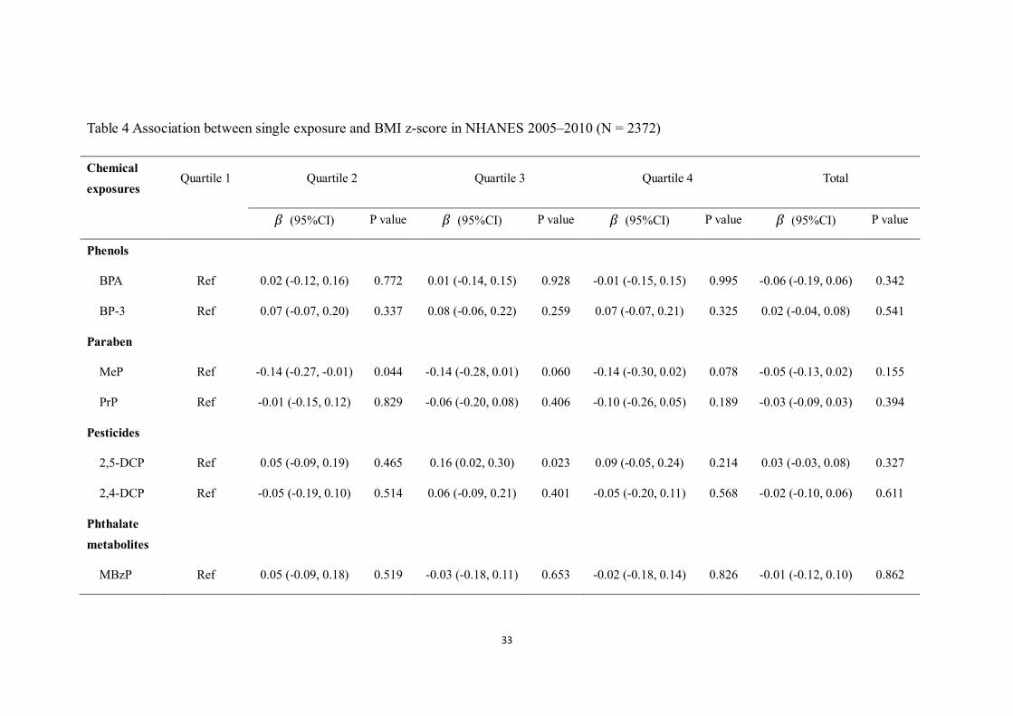
Table 4 Association between single exposure and BMI z-score in NHANES 2005–2010 (N = 2372)

Chemical

exposures Quartile 1 Quartile 2 Quartile 3 Quartile 4 Total

𝛽 (95%CI) P value 𝛽 (95%CI) P value 𝛽 (95%CI) P value 𝛽 (95%CI) P value

Phenols

BPA Ref 0.02 (-0.12, 0.16) 0.772 0.01 (-0.14, 0.15) 0.928 -0.01 (-0.15, 0.15) 0.995 -0.06 (-0.19, 0.06) 0.342

BP-3 Ref 0.07 (-0.07, 0.20) 0.337 0.08 (-0.06, 0.22) 0.259 0.07 (-0.07, 0.21) 0.325 0.02 (-0.04, 0.08) 0.541

Paraben

MeP Ref -0.14 (-0.27, -0.01) 0.044 -0.14 (-0.28, 0.01) 0.060 -0.14 (-0.30, 0.02) 0.078 -0.05 (-0.13, 0.02) 0.155

PrP Ref -0.01 (-0.15, 0.12) 0.829 -0.06 (-0.20, 0.08) 0.406 -0.10 (-0.26, 0.05) 0.189 -0.03 (-0.09, 0.03) 0.394

Pesticides

2,5-DCP Ref 0.05 (-0.09, 0.19) 0.465 0.16 (0.02, 0.30) 0.023 0.09 (-0.05, 0.24) 0.214 0.03 (-0.03, 0.08) 0.327

2,4-DCP Ref -0.05 (-0.19, 0.10) 0.514 0.06 (-0.09, 0.21) 0.401 -0.05 (-0.20, 0.11) 0.568 -0.02 (-0.10, 0.06) 0.611

Phthalate

metabolites

MBzP Ref 0.05 (-0.09, 0.18) 0.519 -0.03 (-0.18, 0.11) 0.653 -0.02 (-0.18, 0.14) 0.826 -0.01 (-0.12, 0.10) 0.862

34

MEP Ref 0.02 (-0.12, 0.16) 0.773 0.12 (-0.03, 0.27) 0.108 0.14 (-0.02, 0.30) 0.083 0.12 (0.02, 0.21) 0.017

MiBP Ref 0.14 (-0.01, 0.28) 0.054 0.07 (-0.08, 0.22) 0.376 0.10 (-0.07, 0.27) 0.251 0.05 (-0.08, 0.18) 0.471

NHANES: National Health and Nutrition Examination Survey; CI: confidence interval; Total means continuous chemical variable. Multivariable

linear regression was conducted and regression coefficients (𝛽) were calculated while comparing the second, third and fourth quartiles of each

chemical with reference to the first exposure quartile (N = 2372). Models were adjusted for age, gender, race, educational levels, family

income-to-poverty ratio, caloric intake, serum cotinine, and log-transformed creatinine.

35

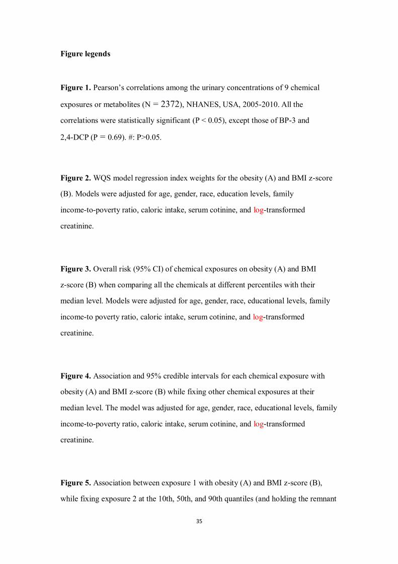
Figure legends

Figure 1. Pearson’s correlations among the urinary concentrations of 9 chemical

exposures or metabolites (N = 2372), NHANES, USA, 2005-2010. All the

correlations were statistically significant (P < 0.05), except those of BP-3 and

2,4-DCP (P = 0.69). #: P>0.05.

Figure 2. WQS model regression index weights for the obesity (A) and BMI z-score

(B). Models were adjusted for age, gender, race, education levels, family

income-to-poverty ratio, caloric intake, serum cotinine, and log-transformed

creatinine.

Figure 3. Overall risk (95% CI) of chemical exposures on obesity (A) and BMI

z-score (B) when comparing all the chemicals at different percentiles with their

median level. Models were adjusted for age, gender, race, educational levels, family

income-to poverty ratio, caloric intake, serum cotinine, and log-transformed

creatinine.

Figure 4. Association and 95% credible intervals for each chemical exposure with

obesity (A) and BMI z-score (B) while fixing other chemical exposures at their

median level. The model was adjusted for age, gender, race, educational levels, family

income-to-poverty ratio, caloric intake, serum cotinine, and log-transformed

creatinine.

Figure 5. Association between exposure 1 with obesity (A) and BMI z-score (B),

while fixing exposure 2 at the 10th, 50th, and 90th quantiles (and holding the remnant

36

predictors to their median level). The models were adjusted for age, gender, race,

educational levels, family income-to-poverty ratio, caloric intake, serum cotinine, and

log-transformed creatinine.

1. Engin A: The Definition and Prevalence of Obesity and Metabolic Syndrome. Advances in

experimental medicine and biology 2017, 960:1-17.

2. Prevalence of obesity among children and adolescents

[https://www.who.int/gho/ncd/risk_factors/overweight_obesity/obesity_adolescents/en/],(a

ccessed 31 October 2019).

3. Simmonds M, Llewellyn A, Owen CG, Woolacott N: Predicting adult obesity from childhood

obesity: a systematic review and meta-analysis. Obesity reviews : an official journal of the

International Association for the Study of Obesity 2016, 17(2):95-107.

4. Twum C, Wei Y: The association between urinary concentrations of dichlorophenol

pesticides and obesity in children. Rev Environ Health 2011, 26(3):215-219.

5. Lavie CJ, De Schutter A, Parto P, Jahangir E, Kokkinos P, Ortega FB, Arena R, Milani RV: Obesity

and Prevalence of Cardiovascular Diseases and Prognosis-The Obesity Paradox Updated.

Progress in cardiovascular diseases 2016, 58(5):537-547.

6. Heindel JJ, Blumberg B, Cave M, Machtinger R, Mantovani A, Mendez MA, Nadal A, Palanza P,

Panzica G, Sargis R et al: Metabolism disrupting chemicals and metabolic disorders.

Reproductive toxicology (Elmsford, NY) 2017, 68:3-33.

7. Kim JT, Lee HK: Childhood obesity and endocrine disrupting chemicals. Annals of pediatric

endocrinology & metabolism 2017, 22(4):219-225.

8. Karoutsou E, Polymeris A: Environmental endocrine disruptors and obesity. Endocrine

regulations 2012, 46(1):37-46.

9. Nadal A, Quesada I, Tuduri E, Nogueiras R, Alonso-Magdalena P: Endocrine-disrupting

chemicals and the regulation of energy balance. Nature reviews Endocrinology 2017,

13(9):536-546.

37

10. Liu B, Lehmler HJ, Sun Y, Xu G, Liu Y, Zong G, Sun Q, Hu FB, Wallace RB, Bao W: Bisphenol A

substitutes and obesity in US adults: analysis of a population-based, cross-sectional study.

The Lancet Planetary health 2017, 1(3):e114-e122.

11. Deierlein AL, Wolff MS, Pajak A, Pinney SM, Windham GC, Galvez MP, Silva MJ, Calafat AM,

Kushi LH, Biro FM et al: Longitudinal Associations of Phthalate Exposures During Childhood

and Body Size Measurements in Young Girls. Epidemiology 2016, 27(4):492-499.

12. Quiros-Alcala L, Buckley JP, Boyle M: Parabens and measures of adiposity among adults and

children from the U.S. general population: NHANES 2007-2014. International journal of

hygiene and environmental health 2018, 221(4):652-660.

13. Xia B, Zhu Q, Zhao Y, Ge W, Zhao Y, Song Q, Zhou Y, Shi H, Zhang Y: Phthalate exposure and

childhood overweight and obesity: Urinary metabolomic evidence. Environment

international 2018, 121(Pt 1):159-168.

14. Park H, Kim K: Concentrations of 2,4-Dichlorophenol and 2,5-Dichlorophenol in Urine of

Korean Adults. International journal of environmental research and public health 2018, 15(4).

15. Bui TT, Giovanoulis G, Cousins AP, Magner J, Cousins IT, de Wit CA: Human exposure, hazard

and risk of alternative plasticizers to phthalate esters. The Science of the total environment

2016, 541:451-467.

16. Dodge LE, Kelley KE, Williams PL, Williams MA, Hernandez-Diaz S, Missmer SA, Hauser R:

Medications as a source of paraben exposure. Reproductive toxicology (Elmsford, NY) 2015,

52:93-100.

17. Shoaff J, Papandonatos GD, Calafat AM, Ye X, Chen A, Lanphear BP, Yolton K, Braun JM:

Early-Life Phthalate Exposure and Adiposity at 8 Years of Age. Environ Health Perspect 2017,

125(9):097008.

18. Buckley JP, Engel SM, Mendez MA, Richardson DB, Daniels JL, Calafat AM, Wolff MS, Herring

AH: Prenatal Phthalate Exposures and Childhood Fat Mass in a New York City Cohort.

Environmental health perspectives 2016, 124(4):507-513.

19. Wang H, Zhou Y, Tang C, He Y, Wu J, Chen Y, Jiang Q: Urinary phthalate metabolites are

associated with body mass index and waist circumference in Chinese school children. PloS

one 2013, 8(2):e56800.

20. Valeri L, Mazumdar MM, Bobb JF, Claus Henn B, Rodrigues E, Sharif OIA, Kile ML,

Quamruzzaman Q, Afroz S, Golam M et al: The Joint Effect of Prenatal Exposure to Metal

Mixtures on Neurodevelopmental Outcomes at 20-40 Months of Age: Evidence from Rural

Bangladesh. Environmental health perspectives 2017, 125(6):067015.

21. Warner M, Rauch S, Coker ES, Harley K, Kogut K, Sjodin A, Eskenazi B: Obesity in relation to

serum persistent organic pollutant concentrations in CHAMACOS women. Environ Epidemiol

38

2018, 2(4).

22. Bobb JF, Claus Henn B, Valeri L, Coull BA: Statistical software for analyzing the health effects

of multiple concurrent exposures via Bayesian kernel machine regression. Environmental

health : a global access science source 2018, 17(1):67.

23. Bobb JF, Valeri L, Claus Henn B, Christiani DC, Wright RO, Mazumdar M, Godleski JJ, Coull BA:

Bayesian kernel machine regression for estimating the health effects of multi-pollutant

mixtures. Biostatistics (Oxford, England) 2015, 16(3):493-508.

24. Sample Design [https://wwwn.cdc.gov/nchs/nhanes/tutorials/module2.aspx],(accessed 1

April 2020).

25. Barr DB, Wilder LC, Caudill SP, Gonzalez AJ, Needham LL, Pirkle JL: Urinary creatinine

concentrations in the U.S. population: implications for urinary biologic monitoring

measurements. Environmental health perspectives 2005, 113(2):192-200.

26. Laboratory Procedure Manual (Method No: 6301.01 )

[https://wwwn.cdc.gov/nchs/data/nhanes/2009-2010/labmethods/PP_F_met_phenols.pdf],(

accessed 31 October 2019).

27. Laboratory Procedure Manual (Method No: 6306.03)

[https://wwwn.cdc.gov/nchs/data/nhanes/2009-2010/labmethods/PHTHTE_F_met.pdf],(acc

essed 31 October 2019).

28. A SAS Program for the 2000 CDC Growth Charts (ages 0 to <20 years)

[https://www.cdc.gov/nccdphp/dnpao/growthcharts/resources/sas.htm],(accessed 31

October 2019).

29. Defining Childhood Obesity

[https://www.cdc.gov/obesity/childhood/defining.html],(accessed 31 March 2020).

30. 2010 Dietary Guidelines [https://health.gov/dietaryguidelines/2010/],(accessed 31 October

2019).

31. Carrico C, Gennings C, Wheeler DC, Factor-Litvak P: Characterization of Weighted Quantile

Sum Regression for Highly Correlated Data in a Risk Analysis Setting. J Agric Biol Environ

Stat 2014, 20(1):100-120.

32. Warner M, Ye M, Harley K, Kogut K, Bradman A, Eskenazi B: Prenatal DDT exposure and child

adiposity at age 12: The CHAMACOS study. Environmental research 2017, 159:606-612.

33. Bhandari R, Xiao J, Shankar A: Urinary bisphenol A and obesity in U.S. children. American

journal of epidemiology 2013, 177(11):1263-1270.

34. Czarnota J, Gennings C, Colt JS, De Roos AJ, Cerhan JR, Severson RK, Hartge P, Ward MH,

Wheeler DC: Analysis of Environmental Chemical Mixtures and Non-Hodgkin Lymphoma

39

Risk in the NCI-SEER NHL Study. Environmental health perspectives 2015, 123(10):965-970.

35. Goodman M, Lakind JS, Mattison DR: Do phthalates act as obesogens in humans? A

systematic review of the epidemiological literature. Crit Rev Toxicol 2014, 44(2):151-175.

36. Jacobson MH, Woodward M, Bao W, Liu B, Trasande L: Urinary Bisphenols and Obesity

Prevalence Among U.S. Children and Adolescents. J Endocr Soc 2019, 3(9):1715-1726.

37. Liu B, Lehmler HJ, Sun Y, Xu G, Sun Q, Snetselaar LG, Wallace RB, Bao W: Association of

Bisphenol A and Its Substitutes, Bisphenol F and Bisphenol S, with Obesity in United States

Children and Adolescents. Diabetes Metab J 2019, 43(1):59-75.

38. Bailey-Davis L, Peyer KL, Fang Y, Kim JK, Welk GJ: Effects of Enhancing School-Based Body

Mass Index Screening Reports with Parent Education on Report Utility and Parental Intent

To Modify Obesity Risk Factors. Childhood obesity (Print) 2017, 13(2):164-171.