using themis spectral data - themis.mars.asu.edu filespectral analysis (1) quantify spectral...
TRANSCRIPT
Using THEMIS spectral data
Deanne Rogers* and Josh Bandfield
*California Institute of TechnologyMC 150-21
Pasadena, CA [email protected]

Overview
• Image selection; evaluating spectralvariability within your study region
• Spectral analysis; defining/interpretingspectral units
• Mapping spectral units and furthercharacterization
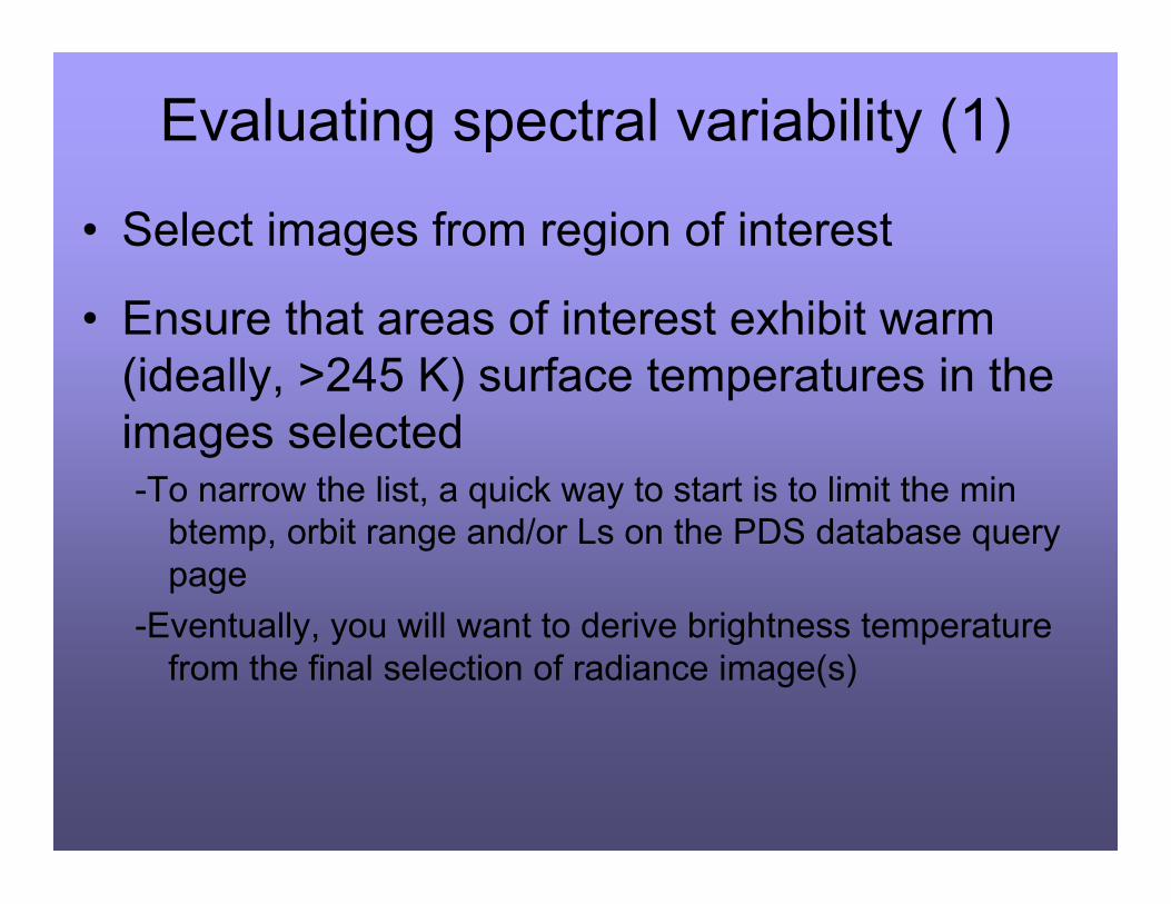
Evaluating spectral variability (1)
• Select images from region of interest
• Ensure that areas of interest exhibit warm(ideally, >245 K) surface temperatures in theimages selected-To narrow the list, a quick way to start is to limit the min
btemp, orbit range and/or Ls on the PDS database querypage
-Eventually, you will want to derive brightness temperaturefrom the final selection of radiance image(s)
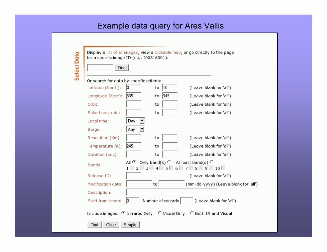
Example data query for Ares Vallis
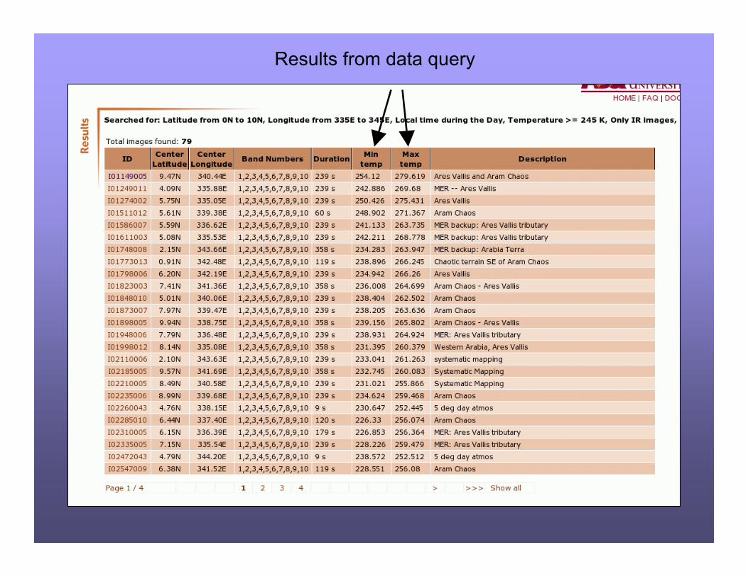
Results from data query
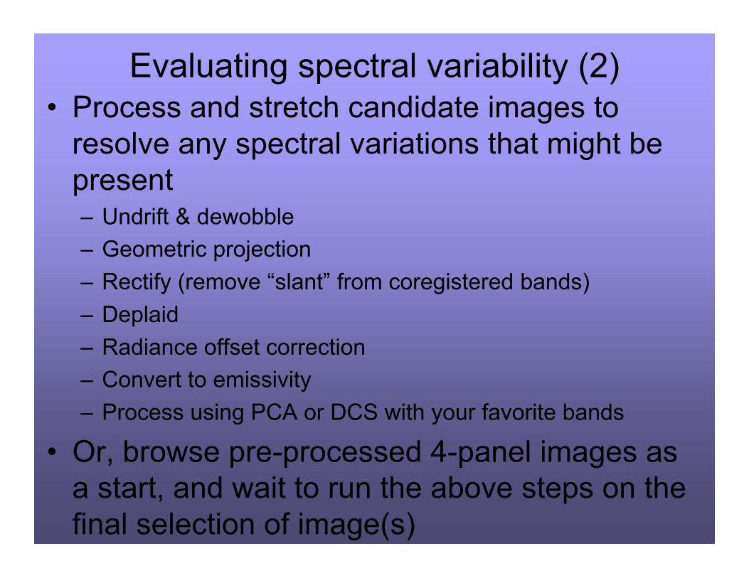
Evaluating spectral variability (2)• Process and stretch candidate images to
resolve any spectral variations that might bepresent– Undrift & dewobble– Geometric projection– Rectify (remove “slant” from coregistered bands)– Deplaid– Radiance offset correction– Convert to emissivity– Process using PCA or DCS with your favorite bands
• Or, browse pre-processed 4-panel images asa start, and wait to run the above steps on thefinal selection of image(s)
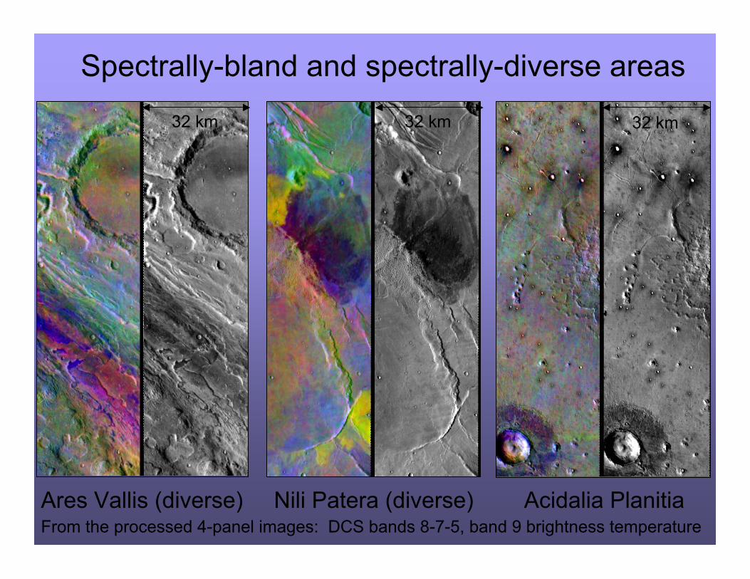
Spectrally-bland and spectrally-diverse areas
Ares Vallis (diverse) Nili Patera (diverse) Acidalia PlanitiaFrom the processed 4-panel images: DCS bands 8-7-5, band 9 brightness temperature
32 km 32 km 32 km
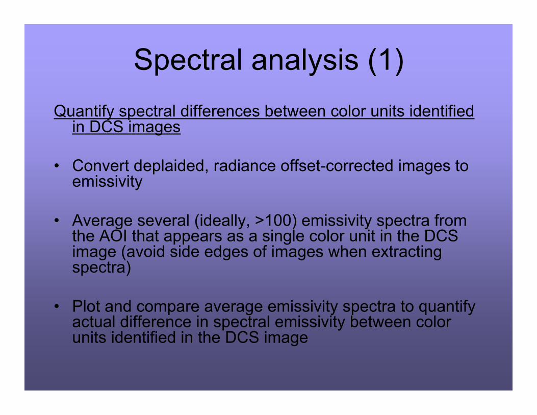
Spectral analysis (1)Quantify spectral differences between color units identified
in DCS images
• Convert deplaided, radiance offset-corrected images toemissivity
• Average several (ideally, >100) emissivity spectra fromthe AOI that appears as a single color unit in the DCSimage (avoid side edges of images when extractingspectra)
• Plot and compare average emissivity spectra to quantifyactual difference in spectral emissivity between colorunits identified in the DCS image
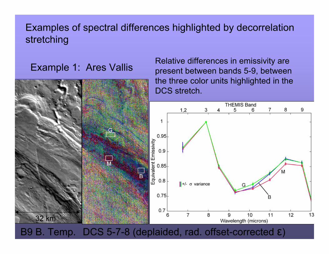
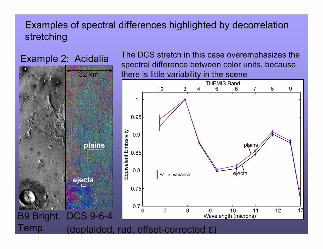
Examples of spectral differences highlighted by decorrelationstretching
Example 1: Ares Vallis
DCS 5-7-8 (deplaided, rad. offset-corrected ε)B9 B. Temp.
Relative differences in emissivity arepresent between bands 5-9, betweenthe three color units highlighted in theDCS stretch.
32 km
plains
ejecta
DCS 9-6-4 (deplaided, rad. offset-corrected ε)
B9 Bright. Temp.
Example 2: Acidalia The DCS stretch in this case overemphasizes thespectral difference between color units, becausethere is little variability in the scene
Examples of spectral differences highlighted by decorrelationstretching
32 km
Spectral analysis (2)
Understanding the spectral differencesbetween color units
• Compositional (surface)?• Variable water ice (atmosphere)?• Variable dust (atmosphere)? unlikely if
surfaces are near each other in horizontaldistance and elevation
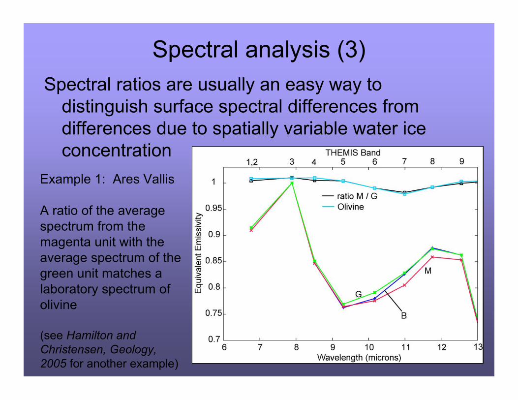
Spectral analysis (3)Spectral ratios are usually an easy way to
distinguish surface spectral differences fromdifferences due to spatially variable water iceconcentration
Example 1: Ares Vallis
A ratio of the averagespectrum from themagenta unit with theaverage spectrum of thegreen unit matches alaboratory spectrum ofolivine
(see Hamilton andChristensen, Geology,2005 for another example)
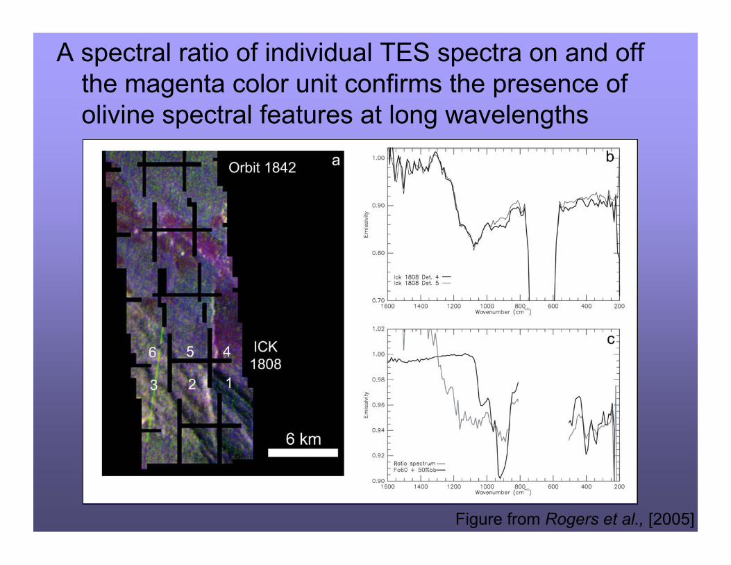
A spectral ratio of individual TES spectra on and offthe magenta color unit confirms the presence ofolivine spectral features at long wavelengths
Figure from Rogers et al., [2005]
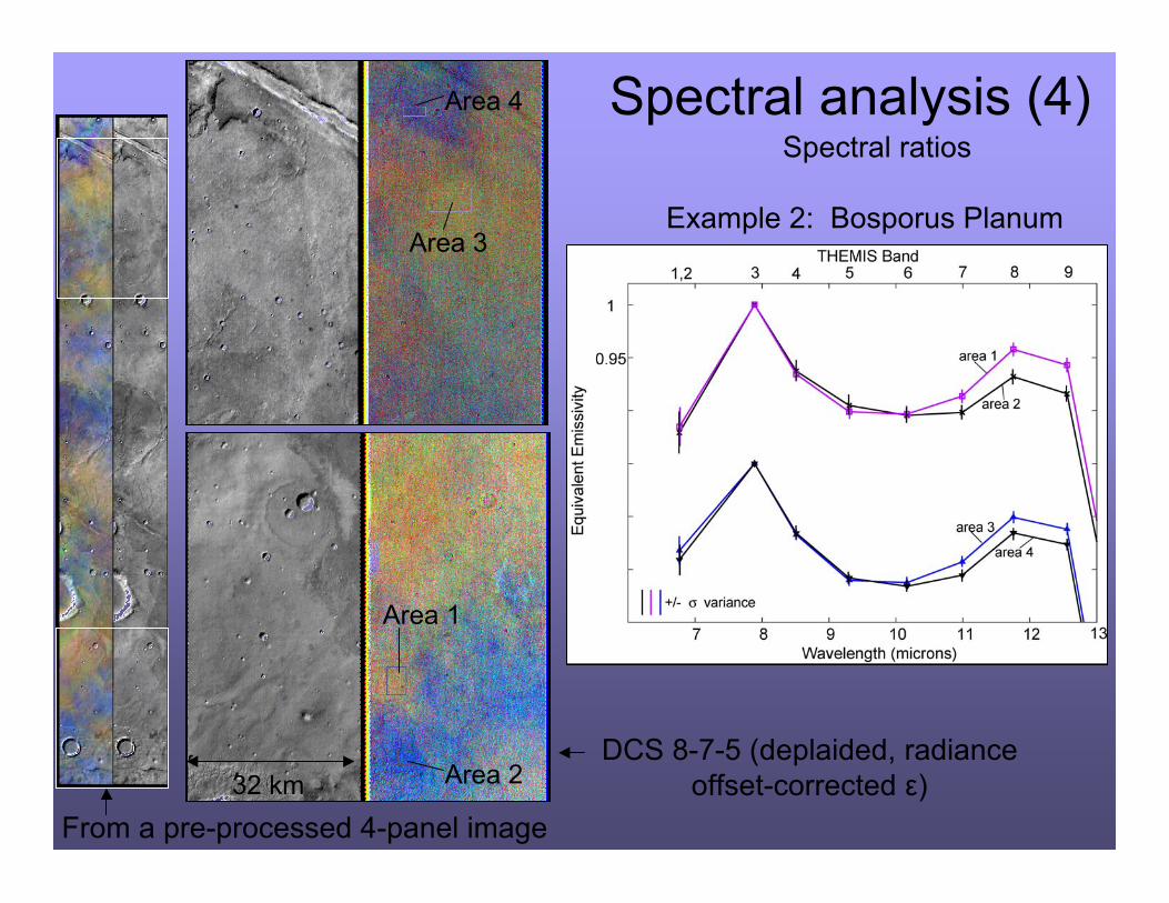
Spectral ratios
Example 2: Bosporus Planum
Spectral analysis (4)
32 km Area 2
Area 1
Area 4
Area 3
DCS 8-7-5 (deplaided, radianceoffset-corrected ε)
From a pre-processed 4-panel image
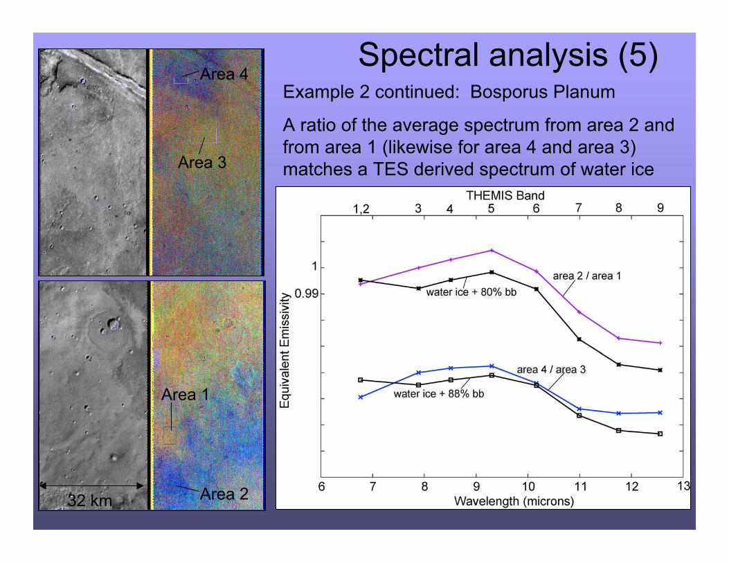
Example 2 continued: Bosporus Planum
Spectral analysis (5)
A ratio of the average spectrum from area 2 andfrom area 1 (likewise for area 4 and area 3)matches a TES derived spectrum of water ice
32 km Area 2
Area 1
Area 4
Area 3
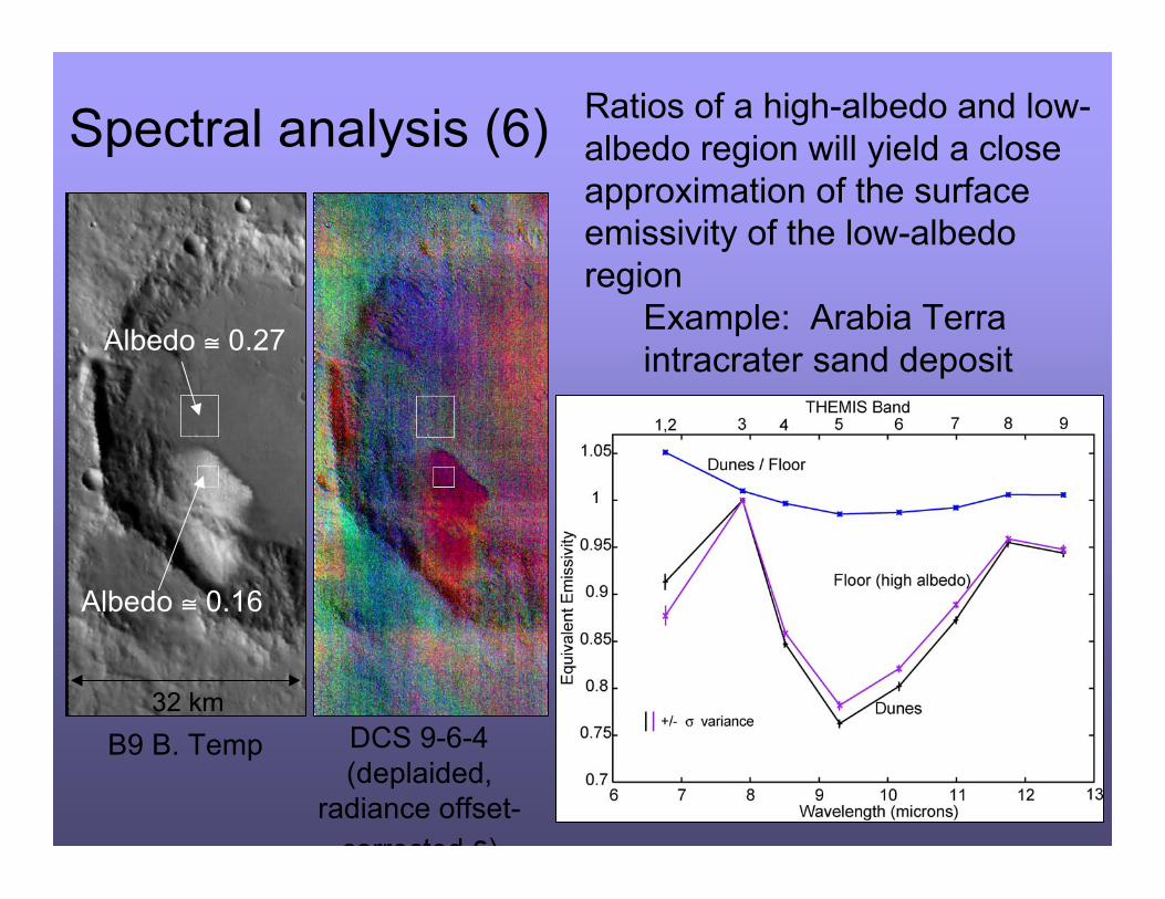
Spectral analysis (6) Ratios of a high-albedo and low-albedo region will yield a closeapproximation of the surfaceemissivity of the low-albedoregion Example: Arabia Terra intracrater sand depositAlbedo ≅ 0.27
B9 B. Temp DCS 9-6-4(deplaided,
radiance offset-corrected ε)
Albedo ≅ 0.16
32 km
If surface emissivity is a desired quantity:1. Find spectrally uniform area within the image that is near the
area(s) of interest in elevation and spatial distance2. Determine surface emissivity of the uniform area using TES data3. Convolve the TES surface emissivity spectrum to THEMIS
spectral bandpasses4. Divide the average THEMIS emissivity of uniform area by the
degraded TES emissivity spectrum to derive the atmospheric component 5. Assume the atmospheric component is constant, and divide this from the entire image (or the image portion of interest)
This method does not remove small-scale spatial variations in water iceconcentrations
If the spectrally uniform area is a high-albedo region, the surface dustendmember derived from EPF observations may be used in lieu of step 2
Spectral analysis (7)
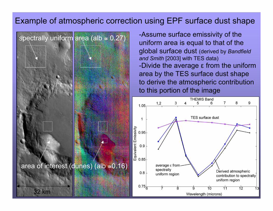
Example of atmospheric correction using EPF surface dust shape
spectrally uniform area (alb ≅ 0.27) -Assume surface emissivity of theuniform area is equal to that of theglobal surface dust (derived by Bandfieldand Smith [2003] with TES data)-Divide the average ε from the uniformarea by the TES surface dust shapeto derive the atmospheric contributionto this portion of the image
area of interest (dunes) (alb ≅0.16)
32 km
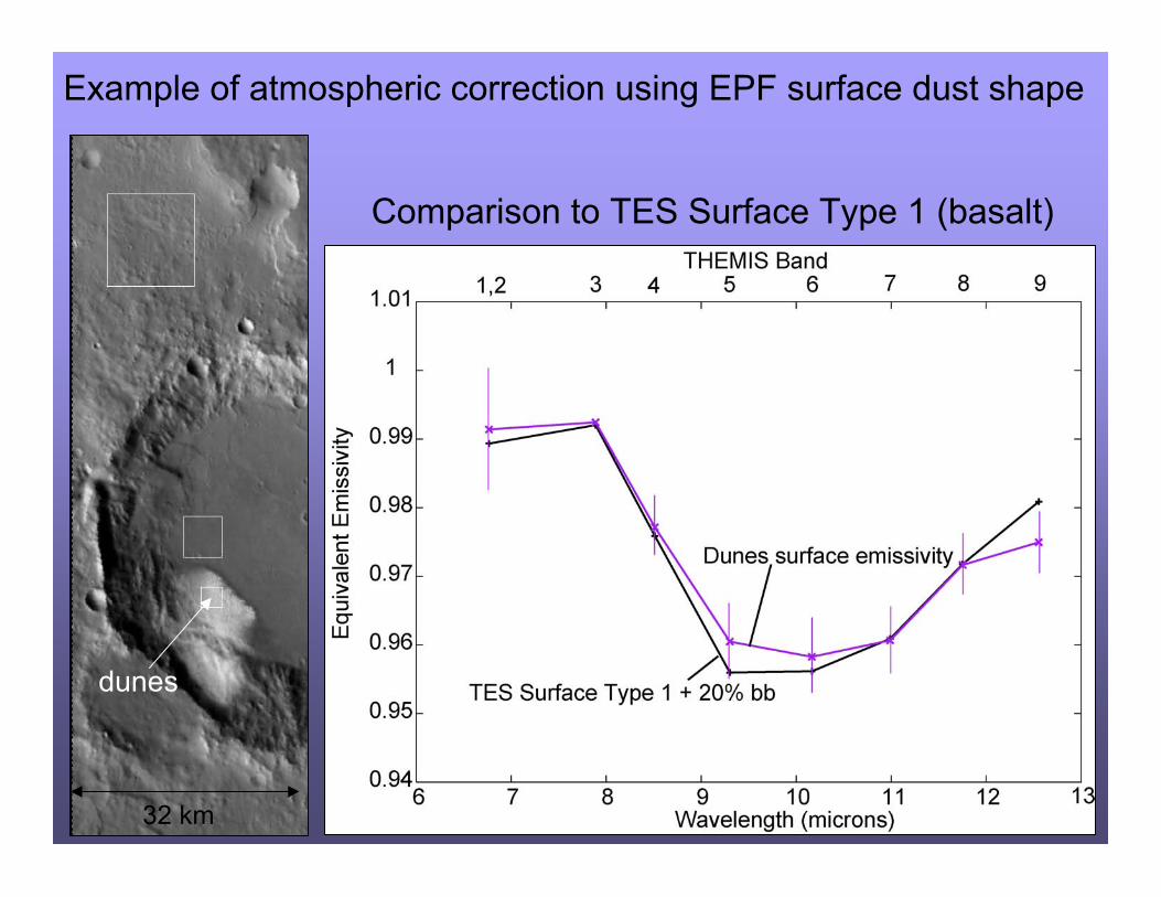
Example of atmospheric correction using EPF surface dust shape
Comparison to TES Surface Type 1 (basalt)
dunes
32 km
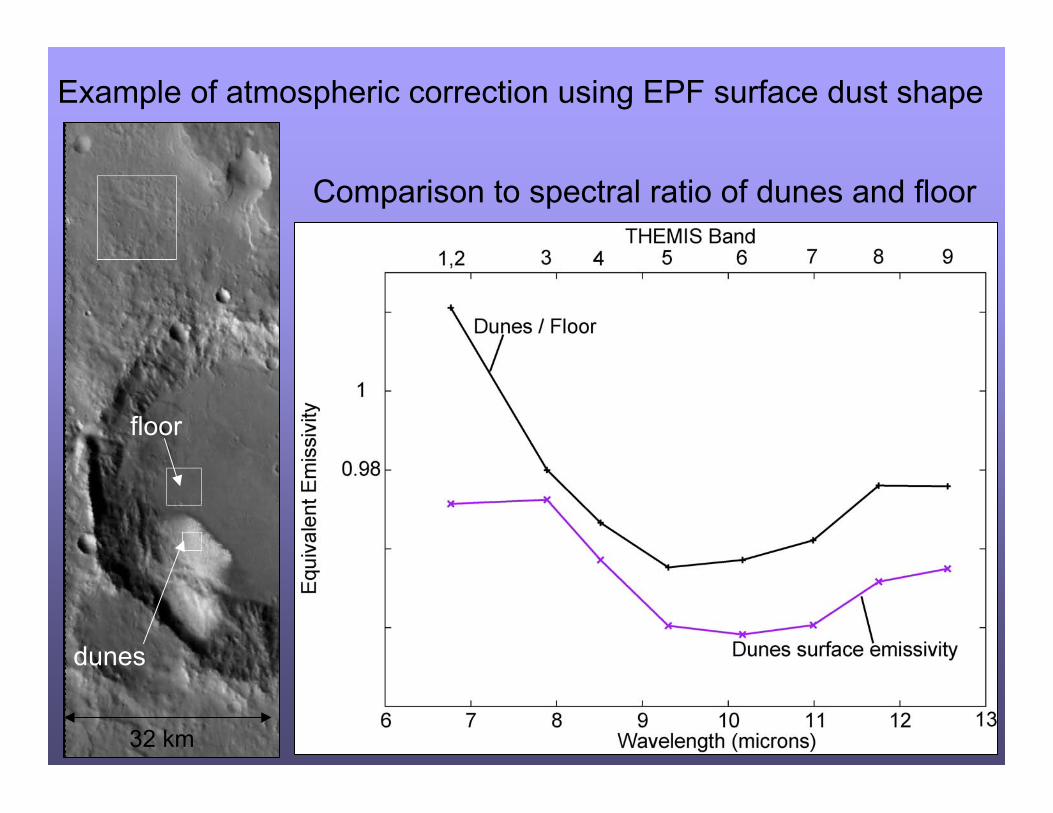
Example of atmospheric correction using EPF surface dust shape
Comparison to spectral ratio of dunes and floor
floor
dunes
32 km
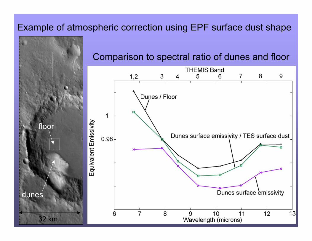
Example of atmospheric correction using EPF surface dust shape
Comparison to spectral ratio of dunes and floor
floor
dunes
32 km
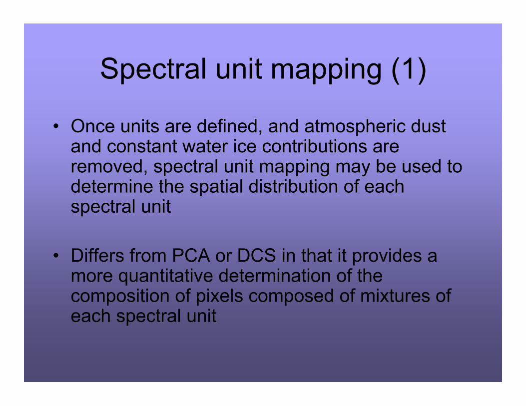
Spectral unit mapping (1)
• Once units are defined, and atmospheric dustand constant water ice contributions areremoved, spectral unit mapping may be used todetermine the spatial distribution of eachspectral unit
• Differs from PCA or DCS in that it provides amore quantitative determination of thecomposition of pixels composed of mixtures ofeach spectral unit
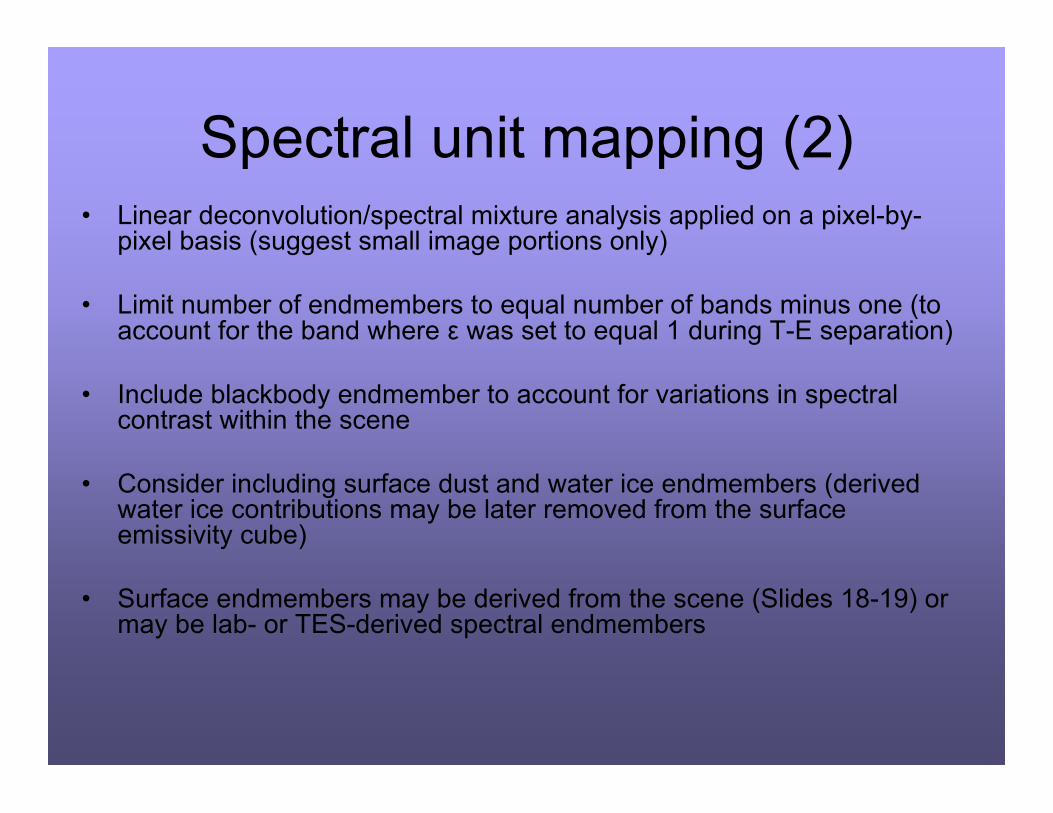
Spectral unit mapping (2)• Linear deconvolution/spectral mixture analysis applied on a pixel-by-
pixel basis (suggest small image portions only)
• Limit number of endmembers to equal number of bands minus one (toaccount for the band where ε was set to equal 1 during T-E separation)
• Include blackbody endmember to account for variations in spectralcontrast within the scene
• Consider including surface dust and water ice endmembers (derivedwater ice contributions may be later removed from the surfaceemissivity cube)
• Surface endmembers may be derived from the scene (Slides 18-19) ormay be lab- or TES-derived spectral endmembers
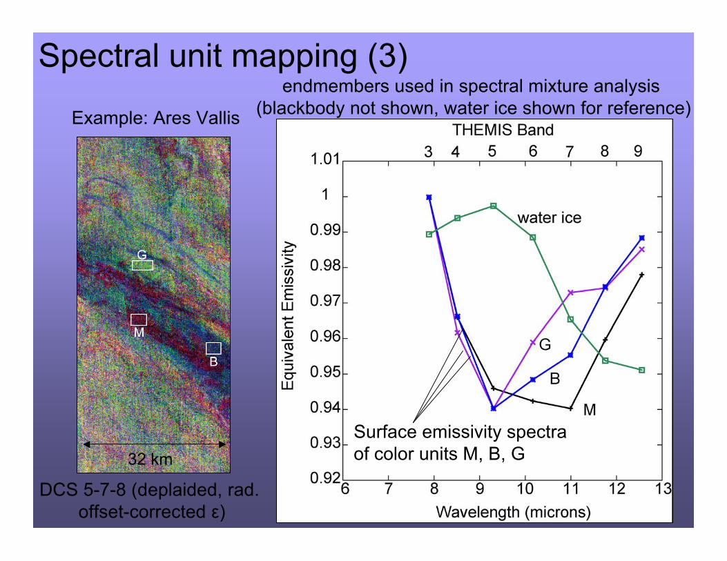
Spectral unit mapping (3)
Example: Ares Vallis
Surface emissivity spectra of color units M, B, G
DCS 5-7-8 (deplaided, rad. offset-corrected ε)
endmembers used in spectral mixture analysis (blackbody not shown, water ice shown for reference)
32 km
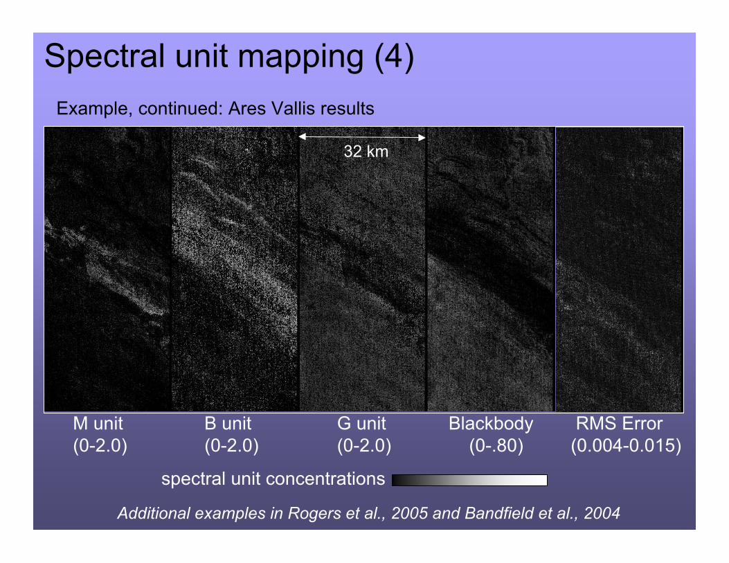
Spectral unit mapping (4)
M unit(0-2.0)
B unit(0-2.0)
G unit(0-2.0)
Blackbody (0-.80)
RMS Error (0.004-0.015)
spectral unit concentrations
32 km
Additional examples in Rogers et al., 2005 and Bandfield et al., 2004
Example, continued: Ares Vallis results
Further characterize spectral units
• May reconstitute (return to original projection)processed data (such as DCS emissivity, orspectral unit concentration maps)
• Processed, reconstituted data may bereincorporated into a GIS
• May need to shift data for small offsets betweendata products
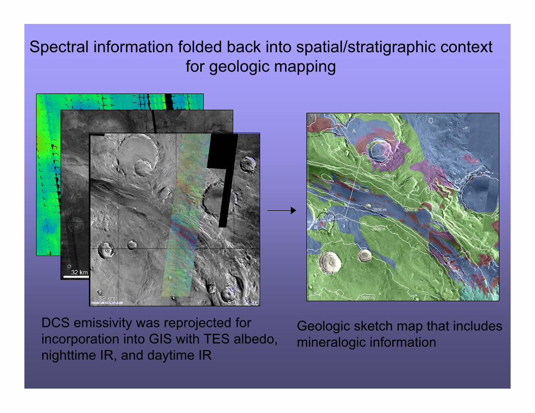
Spectral information folded back into spatial/stratigraphic context for geologic mapping
DCS emissivity was reprojected forincorporation into GIS with TES albedo,nighttime IR, and daytime IR
Geologic sketch map that includesmineralogic information
Other notes• It is informative to examine multiple images over
the area of interest
• It is helpful to work on small portions (example,< 3000 lines at a time) of image for memory-intensive processes (emissivity, spectral unitmapping)
• Avoid side edges of rectified images (~30 pixels oneach side) when extracting spectra
Some references 1. DCS
Gillespie, A. R., Remote Sens. Env., 42, 147-155, 1992
2. Spectral mixture analysis of multispectral images Gillespie, A. R., Remote Sens. Env., 42, 137-145, 1992
Ramsey, M. S., JGR-Planets, 107 (E8), doi:10.1029/2001JE001827
3. THEMIS atm correction and spectral unit mapping techniqes discussed in this presentation and applied examples: Bandfield, J. L.et al., 2004, JGR-Planets, 109(E10), doi:10.1029/2004JE002289
Bandfield, J. L.et al., 2004, JGR-Planets, 109(E10), doi:10.1029/2004JE002290 Christensen, P. R. et al., 2005, Nature, 436(28), 504-509. Rogers, A. D. et al., 2005, JGR-Planets, 110(E5), doi:10.1029/2005JE002399
4. Spectral ratios with TES and THEMIS and applied examples:
Ruff and Christensen, 2002, JGR-Planets, 107(E12), doi:10.1029/2001JE001580 Hamilton and Christensen, 2005, Geology, 33(6), 433-436. Johnson, J. R. et al., 2002, JGR-Planets, 107(E6), doi:10.1029/2000JE001405
5. Derivation of atmospheric endmembers and surface dust endmembers from TES dataBandfield, J. L. et al., 2000, JGR-Planets, 105(E4), 9573-9587Bandfield and Smith, 2003, Icarus, 161(1), 47-65.