Using the SRSim Software for Spatial andRule-Based Modeling of CombinatoriallyComplex Biochemical Reaction Systems

Gerd Gruenert and Peter Dittrich

Jena Center for Bioinformatics, Bio Systems Analysis Group,Institute of Computer Science, Friedrich Schiller University Jena,

Ernst-Abbe-Platz 1-4, D-07743 Jena, Germany{Gerd.Gruenert,Peter.Dittrich}@uni-jena.de

http://www.biosys.uni-jena.de/

Abstract. The simulator software SRSim is presented here. It is con-structed from the molecular dynamics simulator LAMMPS and a setof extensions for modeling rule-based reaction systems. The aim of thissoftware is coping with reaction networks that are combinatorially com-plex as well as spatially inhomogeneous. On the one hand, there is acombinatorial explosion of necessary species and reactions that occurswhen complex biomolecules are allowed to interact, e.g. by polymer-ization or phosphorilation processes. On the other hand, diffusion overlonger distances in the cell as well as the geometric structures of sophis-ticated macromolecules can further influence the dynamic behavior of asystem. Addressing the mentioned demands, the SRSim simulation sys-tem features a stochastic, particle based, spatial simulation of BrownianDynamics in three dimensions of a rule-based reaction system.

Rule-based Modeling in Space

Biological systems exhibit a high number of possible combinations between in-teracting proteins, frequently leading to huge molecules of interconnected pro-tein compounds. Examples would be the complexes assembled for RNA or DNAtranscriptases, ATP synthases [26], mitotic checkpoint networks [18] or the deathinducing signaling complex (DISC) [41]. Next to the resulting complex graphsof interacting proteins, there are post-translational modification to proteins, e.g.from phosphorilations. Basically, each modification pattern defines a new chem-ical species with its unique chemical behavior. Exemplary, this would result in anumber of 227 different species for the tumor suppressor protein p53 which com-prises 27 phosphorilation sites [2]. Such a high number of species poses problemsfor the simulation with (partial) differential equations and stochastic algorithms.But it also becomes very hard to analyze and understand the “mechanics” ofsuch a complex model. A possible remedy for stochastic simulations is discussedhere [35].

Another possible solution to the problem of combinatorial explosion is pro-posed by the domain-oriented approach and rule-based modeling [27, 15, 16,

8, 12]. In this scenario, elementary molecules consist of a set of compo-nents or domains which can be modified or bound to the components of othermolecules. Components, sites, binding sites and domains are used synonymouslyin this article. The resulting complex species, formed from a connection of ele-mentary molecules, are called molecule graphs.

Instead of using reactions between explicit species now, the reactions arereplaced by implicit reaction rules, which are applicable to a certain subsetof all possible complex molecular species. This subset is defined through anequivalence class given by a molecule graph pattern. Any complex moleculegraph that contains the graph pattern as an isomorphic sub-pattern is includedin the equivalence class. A pattern might for example describe a molecule oftype A that has one free binding site and another binding site bound to anothermolecule of type A. Any other molecular species that incorporates this A − Adimer without blocking the necessary free binding site specified in the patternis now part of this equivalence class. Any of these molecules can be addressedby a single reaction rule, as demonstrated in Figure 1.

There is a lot of software available for rule-based modeling, as for exampleStochsim [27], BioNetGen [5], BIOCHAM [10], Moleculizer [23] or Pathway LogicAssistant [39] or Cellucidate. Nonetheless spatial aspects are mostly neglectedin these approaches (except for Stochsim).

Spatial Aspects

Spatiotemporal heterogeneities in reaction systems are generally considered tobe of high importance for many systems [3, 25, 19, 38]. This led to a varietyof spatial simulation techniques, starting from deterministic, population-based,partial differential equations [28] towards stochastic simulation of single particlesin discrete or continuous 3d space [40, 9, 21]. See [22, 38] for an overview on spatialsimulation systems.

Similar to and partially based on the approaches [4, 34, 43, 20, 11, 37], we areusing individual agents for each elementary molecule in the simulation. Syn-onymously with the agents, we are using the terms particles and elementarymolecules here. The spatial simulation is carried out as an extension to themolecular dynamics simulator LAMMPS [31]. Each particle is represented by itsposition, its velocity, its species and the state of its components. The particlesdiffuse through the reactor and can push away other molecules if they cometoo close. When two molecules approach one another, a bimolecular reactioncan happen between them, if they are fitting to a reaction pattern specified inthe reaction rules and if the geometric constraints are met. If a reaction bindstwo elementary molecules together, bond forces are applied and their diffusionthrough the reactor is coupled, forming a complex molecule graph. Monomolec-ular reactions can be used to spontaneously break bonds in molecule graphs orto modify the component states of a molecule. More conventional reactions canalso be used to completely exchange one molecule for another.

The inclusion of spatial aspects in the rule-based reaction systems results inan expressive simulation system for moderately sized systems. Up to 100000 sim-

Ax x

a) elementary molecules withtheir domains

b) examples for complex molecule graphs

By y

z

A A A A B B

A

A

c) exemplary reaction rule:

A A B B+ A A B B

d) exemplary realizations of the rule:

A A AA B B

A

A

(+)

A A AA B B

A

A

B B AA B

B BAAA

B B AA B

B BAAA

+

Fig. 1. Exemplary rule-based system, taken from [13]. Two elementary molecule types(A, B) with their sub domains (or components) are displayed (a). Each componentcan be bound to another component or be modified, e.g. denoting a phosphorylation ora conformational change. Site names need not be unique and hence a wide spectrum ofpossibilities for the system’s specification is offered. Multiple elementary molecules canbe connected at their components to form complex molecule graphs (b). Reactionrules, as the binding reaction (c), are specified by using patterns graphs (or reactantpatterns) A reactant pattern fits to a molecule graph, if it is contained as a subgraphin the molecule graph. Note that some components are missing in the reactant pattern’sdefinition, which are then ignored in the matching process. Panel (d) shows two differentinstances of the reaction rule. In the upper realization, two independent molecule graphsare connected. For the lower example on the other hand, both of the rules’ reactantpatterns are found in a single connected molecule graph.

ulated particles can still be run on a desktop system for about 106 timesteps insome hours of computing time. Though SRSim was designed for the simulationof biological systems, also designing and planning chemical computing experi-ments might be a good application. We simulated for example the formation ofSierpinski triangles [13] following the work of Winfree et al. and Rothemund etal. [42, 33].

Though the SRSim simulation system cannot directly be used to simulateP-Systems [29, 30], there are some parallels to the membrane computing per-spective. Similar to some P-System [24, 32] we are using a stochastic simulationapproach that is based on individual particles in 3d space, though with limitedsupport for the constitution of membranes. That is, if we want to setup an im-plicit diffusion barrier in our system “SRSim”, we can do this by adding forcesto the reactor that confine certain molecules to defined subvolumes inside thereactor. Then, reactions can be used to transfer particles with specified ratesthrough these pseudo-membranes. Nonetheless, that would be a rather awkwardworkaround to the ,,missing” membranes in the SRSim approach. On the otherhand, similar to approaches like [11, 36], the dynamic creation, modification anddestruction of membranes can be reduced to the underlying macromolecularinteractions by simulating lipid molecules that build the membranes.

Another similarity might be that both approaches, the rule-based and themembrane-computing systems, use further constraints on the underlying non-deterministic reaction system. While in membrane computing, there are dynamicmembranes to separate different molecules against interactions, there are the ge-ometry and the complex molecule-graph structure in the SRSim approach thatallows or even favours one kind of reactions and that inhibits other types. Forthe inner workings of biological cells, both types of processes might be equallyimportant. Maybe there could even be seen a hierarchy of first controlling geome-tries of interacting particles on the level of macromolecules and then constrainingthese interactions through the relationship between the compartments. From thecomputational point of view, both types of systems offer a high combinatorialcomplexity, leading to computational capacities as shown for P-Systems [30,36] and for self-assembly systems [1, 33, 7]. When intending to build comput-ing systems from scratch, self-assembling macromolecules as well as structuredmembranes might both supply helpful building blocks.

Though that is not what we present in this paper, it might prove interestingto combine both types of constraints to a single system. This would also openthe possibility to describe geometric relations not only between the particles,but also between the membranes. For the rule-based modelling community onthe other hand, it would certainly be very handy to use the concept of dynamicmembrane formation and decay. In the case of non-spatial simulation and staticmembranes, this was already done [14].

In the following sections, we try not to unfold the complete technical simu-lation process. Instead, the process of setting up and running a simple systemwill be demonstrated from installing the software to setting up and running the

simulation. For the theory behind the spatial and rule-based simulation, pleaserefer to [13].

Installing SRSim

Unfortunately the installation of SRSim is not yet fully automatized, so thereare some uncomplicated steps to do. The following installation instructions areaddressed to x86 linux users, who are assumed to have Gnu Make and a C++compiler installed. No tests were carried out using different hard- or softwareplatforms, but as long as the required libraries are present, no architecture spe-cific code is used.

Required Software

In the first place, make sure that the following libraries are present on yoursystem, namely Xerces-C++1, which is required for XML parsing. The otherdependency is the “Message Passing Interface”2 (MPI), a parallel computingstandard used by LAMMPS. There are different MPI implementations available.

It is recommended but not necessary to install the software “Visual Molec-ular Dynamics”3 (VMD) [17], which can be very helpful to visualize moleculartrajectories calculated by SRSim.

Compiling SRSim

To build a SRSim executable, first the Rule System is compiled to a librarythat is later linked against the LAMMPS molecular dynamics simulator sources.After unpacking the SRSim distribution to a directory X, this should basicallybe done by invoking make lmp srsim in the directory X/source of the SRSimdistribution. This will create the library, build the tool createGeo and thencompile LAMMPS with the additional modules necessary for SRSim.

If the MPI and Xerces libraries are not in the standard paths for includeand library files, you have to modify the -I and -L paths in the makefilesX/source/lammpsCompilation/Makefile and X/source/RuleSys/Makefile.

After the successful compilation, two new executables,X/source/lammpsCompilation/lmp srsim and X/source/RuleSys/createGeocan be found. You have to copy or link these files to a place in your system that isin your search path, as for example /usr/local/bin or∼/bin. If you do not havea special directory for executables, you can just add the LAMMPS compilation

1 download from http://xerces.apache.org/xerces-c/ or use the system’s packetmanager. Versions 2.7 and 2.8 seem to work fine.

2 download for example MPICH fromhttp://www.mcs.anl.gov/research/projects/mpich2/ or use your system’s packetmanager.

3 download from http://www.ks.uiuc.edu/Research/vmd/

Fig. 2. Overview of the input / output file structure of SRSim.

directory directly to your search path by editing ∼/.bashrc and adding a lineexport PATH=$PATH:X/source/lammpsCompilation:X/source/RuleSys.

If the command lmp srsim outputs the following line, you are done installingSRSim.

LAMMPS (7 Jul 2009)

Here, the 7th July 2009 is the LAMMPS version, that SRSim was built upon.

Using the Software

The molecular dynamics simulator LAMMPS is a script-driven command lineprogram. Since SRSim is no autonomous tool, but an extension to LAMMPS,it is started in the same way as the Molecular Dynamics simulator: lmp srsim< input script.in. The LAMMPS input script *.in is then referencing threeother input files and two or more output files as illustrated in Figure 2. Thereferenced input files are the *.bngl file, specifying the used rule-based reac-tion system, the *.geo file for the molecular geometry definition and finally the*.tgeo file for the template geometry definition. The output files will usuallybe a *.srsim.gdat file containing the concentrations of the observed speciesand a *.lammpstrj file with all the molecular coordinates, which can be usedto visualize and to analyze the simulation run in detail.

To observe the results, gnuplot and VMD can be used. Typevmd output.lammpstrj for instance, to see a graphic representation of the re-action volume. Though VMD (See Section 1) was rather designed to displayall-atom systems, it can be customized neatly and various helper scripts can befound on the Internet.

An Exemplary System

Let us assume we try to build a simple simulation with two elementary molecules.Species A will be a polymerizing molecule that requires energy provided by amolecule B to further polymerize. To allow a linear polymerization for moleculesof type A, two opposing components a and c are introduced. A third component

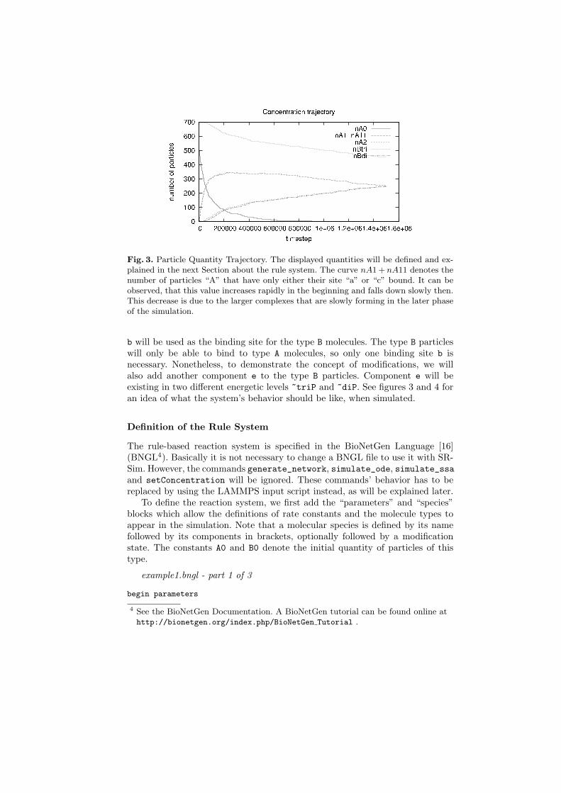
Fig. 3. Particle Quantity Trajectory. The displayed quantities will be defined and ex-plained in the next Section about the rule system. The curve nA1 + nA11 denotes thenumber of particles “A” that have only either their site “a” or “c” bound. It can beobserved, that this value increases rapidly in the beginning and falls down slowly then.This decrease is due to the larger complexes that are slowly forming in the later phaseof the simulation.

b will be used as the binding site for the type B molecules. The type B particleswill only be able to bind to type A molecules, so only one binding site b isnecessary. Nonetheless, to demonstrate the concept of modifications, we willalso add another component e to the type B particles. Component e will beexisting in two different energetic levels ~triP and ~diP. See figures 3 and 4 foran idea of what the system’s behavior should be like, when simulated.

Definition of the Rule System

The rule-based reaction system is specified in the BioNetGen Language [16](BNGL4). Basically it is not necessary to change a BNGL file to use it with SR-Sim. However, the commands generate_network, simulate_ode, simulate_ssaand setConcentration will be ignored. These commands’ behavior has to bereplaced by using the LAMMPS input script instead, as will be explained later.

To define the reaction system, we first add the “parameters” and “species”blocks which allow the definitions of rate constants and the molecule types toappear in the simulation. Note that a molecular species is defined by its namefollowed by its components in brackets, optionally followed by a modificationstate. The constants A0 and B0 denote the initial quantity of particles of thistype.

example1.bngl - part 1 of 3

begin parameters

4 See the BioNetGen Documentation. A BioNetGen tutorial can be found online athttp://bionetgen.org/index.php/BioNetGen Tutorial .

Fig. 4. A scene rendered from the reactor with VMD after 500000 timesteps. shortmultimerizations of two to four A-B dimers can be observed.

k1 1.5e-2

k2 1.5e-2

k3 5e-5

A0 500

B0 700

end parameters

begin species

A(a,b,c) A0

B(b,e~triP) B0

end species

The next block defines which reactions are possible. A first rule is used to bindmolecule A with a free b site to a molecule B with a free b site. The connections oftwo molecules via their components is expressed through the exclamation mark,followed by a common identifier, !1. Since we did not mention any of the sites aor c of molecule A, they can be in any state, free or bound to any other complexmolecule. To allow the polymerization of the A molecules, we need to define thesecond reaction rule. It should state, that a molecule A with a free binding sitea can bind to another molecule A’ with a free binding site a’. But only whenone of them has bound an energy supplying molecule B. The third rule states,that a high-energy molecule B drops down into a lower energy state ~diP, whenthe molecule A it belongs to has no free connection sites any more. Note thatthe binding symbol a!+ marks a site that is bound to any other molecule thatis not explicitly named.

example1.bngl - part 2 of 3

begin reaction rules

1 A(b) + B(b) -> A(b!1).B(b!1) k1

2 A(c) + A(a,b!1).B(b!1,e~triP) -> A(c!2).A(a!2,b!1).B(b!1,e~triP) k2

3 A(a!+,c!+,b!1).B(b!1,e~triP) -> A(a!+,c!+,b!1).B(b!1,e~diP) k3

end reaction rules

For the analysis of the reaction system, a fourth, optional block can be de-fined, listing patterns whose quantities should be output in the simulation. Thismight be for example the numbers of A molecules with no, one or two attachedneighbors, or the numbers of B molecules in the high- or low energy state.

example1.bngl - part 3 of 3

begin observables

Molecules nA0 A(a,c)

Molecules nA1 A(a,c!+)

Molecules nA11 A(a!+,c)

Molecules nA2 A(a!+,c!+)

Molecules nBtri B(e~triP)

Molecules nBdi B(e~diP)

end observables

Molecule and Template Geometry Files

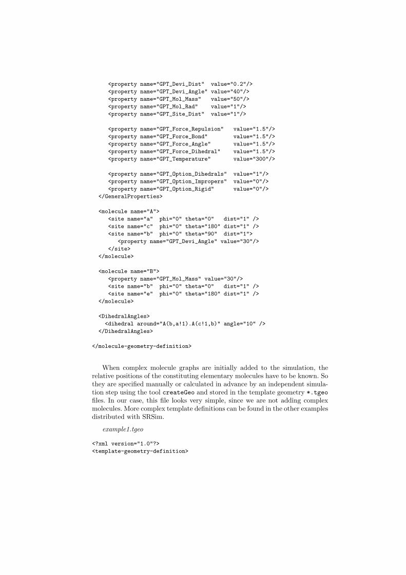
Now that the reaction system is defined, we have to specify the geometry forthe elementary molecules A and B that we want to use in the *.geo geometryfile. For each species, the mass and radius as well as the attributes for eachcomponent have to be defined. The orientations of the particles’ binding sites areexpressed as spherical coordinates through the angles phi, theta and a distancefrom the particles center. Phi can be imagined as the geographic longitude, whiletheta is similar to the geographic latitude. In contrast to geographic coordinates,theta=0 specifies one pole, 90◦ is the equatorial plane and 180◦ is the other pole.For each elementary molecule type, a molecule section has to be defined. Withinthis, each site that is mentioned in the reaction system has to be represented bya site tag inside the molecule definition.

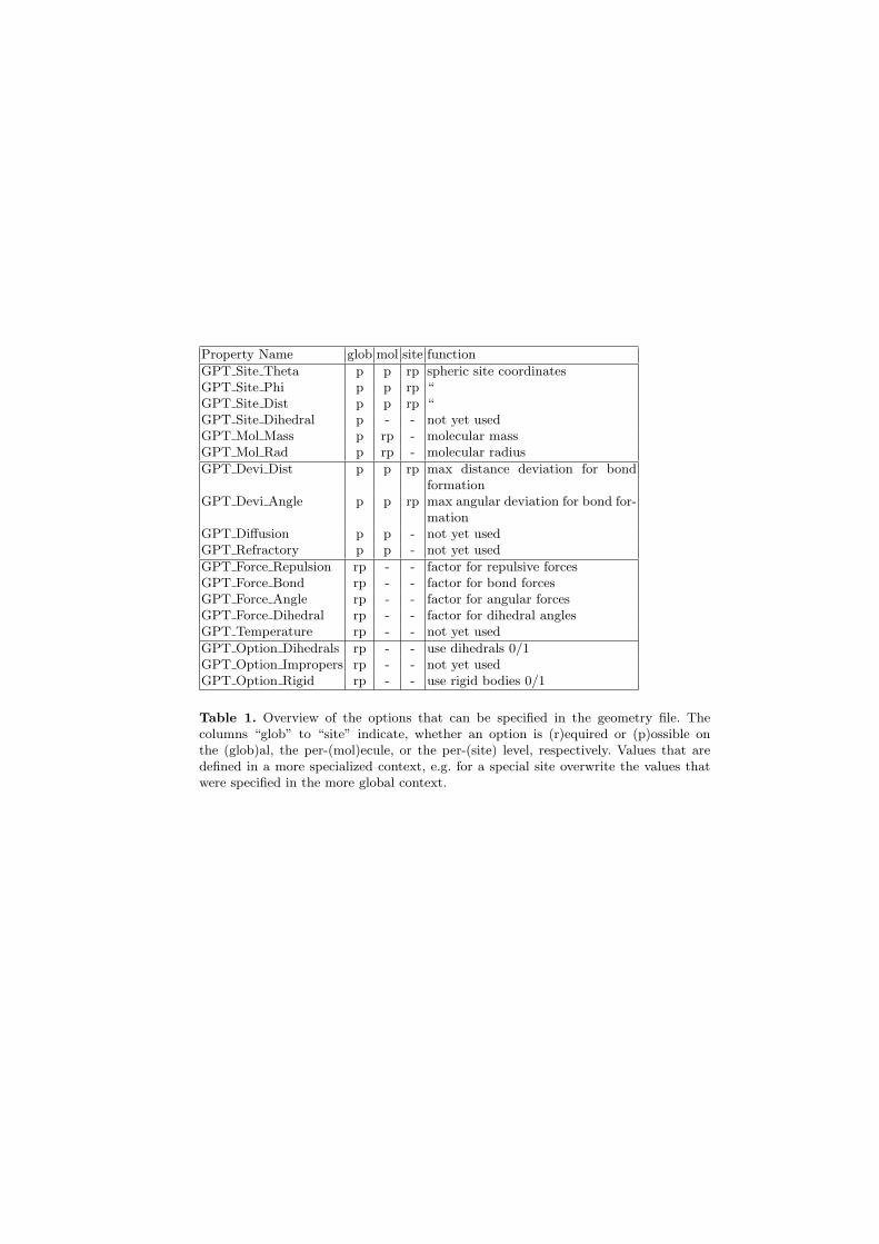
A general section in the beginning of the geometry file lists general propertyvalues for the simulation and values that should be used by default for all theparticles. To specify certain values more individually, property tags can be in-cluded in the molecule and site blocks as well. See Table 1 for a list of propertynames and where they can be used.

A final section DihedralAngles can be used in the geometry definition tospecify dihedral angles for certain bonds.

example1.geo - part 1 of 3

<?xml version="1.0"?>

<molecule-geometry-definition>

<version value="1.01"/>

<GeneralProperties>

Property Name glob mol site function

GPT Site Theta p p rp spheric site coordinatesGPT Site Phi p p rp “GPT Site Dist p p rp “GPT Site Dihedral p - - not yet usedGPT Mol Mass p rp - molecular massGPT Mol Rad p rp - molecular radius

GPT Devi Dist p p rp max distance deviation for bondformation

GPT Devi Angle p p rp max angular deviation for bond for-mation

GPT Diffusion p p - not yet usedGPT Refractory p p - not yet used

GPT Force Repulsion rp - - factor for repulsive forcesGPT Force Bond rp - - factor for bond forcesGPT Force Angle rp - - factor for angular forcesGPT Force Dihedral rp - - factor for dihedral anglesGPT Temperature rp - - not yet used

GPT Option Dihedrals rp - - use dihedrals 0/1GPT Option Impropers rp - - not yet usedGPT Option Rigid rp - - use rigid bodies 0/1

Table 1. Overview of the options that can be specified in the geometry file. Thecolumns “glob” to “site” indicate, whether an option is (r)equired or (p)ossible onthe (glob)al, the per-(mol)ecule, or the per-(site) level, respectively. Values that aredefined in a more specialized context, e.g. for a special site overwrite the values thatwere specified in the more global context.

<property name="GPT_Devi_Dist" value="0.2"/>

<property name="GPT_Devi_Angle" value="40"/>

<property name="GPT_Mol_Mass" value="50"/>

<property name="GPT_Mol_Rad" value="1"/>

<property name="GPT_Site_Dist" value="1"/>

<property name="GPT_Force_Repulsion" value="1.5"/>

<property name="GPT_Force_Bond" value="1.5"/>

<property name="GPT_Force_Angle" value="1.5"/>

<property name="GPT_Force_Dihedral" value="1.5"/>

<property name="GPT_Temperature" value="300"/>

<property name="GPT_Option_Dihedrals" value="1"/>

<property name="GPT_Option_Impropers" value="0"/>

<property name="GPT_Option_Rigid" value="0"/>

</GeneralProperties>

<molecule name="A">

<site name="a" phi="0" theta="0" dist="1" />

<site name="c" phi="0" theta="180" dist="1" />

<site name="b" phi="0" theta="90" dist="1">

<property name="GPT_Devi_Angle" value="30"/>

</site>

</molecule>

<molecule name="B">

<property name="GPT_Mol_Mass" value="30"/>

<site name="b" phi="0" theta="0" dist="1" />

<site name="e" phi="0" theta="180" dist="1" />

</molecule>

<DihedralAngles>

<dihedral around="A(b,a!1).A(c!1,b)" angle="10" />

</DihedralAngles>

</molecule-geometry-definition>

When complex molecule graphs are initially added to the simulation, therelative positions of the constituting elementary molecules have to be known. Sothey are specified manually or calculated in advance by an independent simula-tion step using the tool createGeo and stored in the template geometry *.tgeofiles. In our case, this file looks very simple, since we are not adding complexmolecules. More complex template definitions can be found in the other examplesdistributed with SRSim.

example1.tgeo

<?xml version="1.0"?>

<template-geometry-definition>

<template id="0" name="A(a,b,c)">

<mol id="0" x= "0" y="0" z= "0" />

</template>

<template id="1" name="B(b,e~triP)">

<mol id="0" x= "0" y="0" z= "0" />

</template>

</template-geometry-definition>

The LAMMPS Input Script

The LAMMPS input script is parsed line by line, each of which holds one com-mand modifying the simulation system. Comments can be added using the #sign. Note that the order of the commands is important since the input scriptis parsed from top to bottom. There is a large number of possible commandsthat can be used to customize the simulation, so please refer to the LAMMPSdocumentation5 for further details on the original LAMMPS commands. Thesecommands can for example be used to define custom force terms or to createsimulation outputs in different formats.

example1.in

##

# Phase 1 - setup reactor

##

dimension 3

boundary f f f # use fixed boundary conditions

units real # timescale: fs, distances: Angstrom

newton on

atom_style srsim example1.bngl example1.geo example1.tgeo 11111

########## cmd .bngl .geo .tgeo random_seed

lattice none

region Nucleus block -40 40 -40 40 -40 40 units box

###### dimensions of the reaction volume

create_box 100 Nucleus

# n_atom_types Region_name

start_state_srsim coeffs

start_state_srsim atoms

# set initial values e.g. bond forces etc.

5 The LAMMPS documentation comes together with LAMMPS’ sources and can beaccessed online at http://lammps.sandia.gov/doc/Manual.html.

# and add molecules to the simulation

neighbor 5.0 bin

# size of neighbor-grouping bins

##

# Phase 2 - setup forces

##

fix 1 all langevin 300 300 160.0 12345

# parameters: Temp Temp Gamma^-1 random_seed

fix 2 all nve

fix 3 all wall/reflect xlo xhi ylo yhi zlo zhi

fix 4 all srsim 1 45678 1.0 1.0 1.0 1.0 1.0 50

# fix srsim syntax: fix id group srsim | nEvery randomSeed

# preFactBindR preFactBreakR preFactExchangeR

# preFactModifyR_1 preFactModifyR_2 refractoryTime

##

# Phase 3 - run

##

# Dumps:

thermo 5000 # write themodynamics information every 5k timesteps

timestep 1 # one timestep = 1 fs

dump 1 all atom 1000 example1.lammpstrj

############### trajectory output

dump_modify 1 scale yes

dump 2 all srsim 1000 example1.srsim.gdat

################ concentrations output

# first run phase for 500k ts

run 500000

# second run phase with higher time-resolution

dump_modify 1 every 10

run 5000

In the first phase, some basic parameters have to be set, as for examplethe units to be used, the size of the reaction volume, the maximum number ofmolecular species and the initial configuration of the simulation system. Notethat the command atom_style uses a special atom style, specially designed forSRSim, which is followed by the names of the other input files and the randomseed.

In the second phase, different “fixes” are selected to be applied to the simula-tion. These are computations which influence each molecule’s data, for exampletheir positions, velocities or binding states. The most basic fix, called nve, isthe calculation applied to move each particle according to Newton’s equationsof motion in dependency of the applied forces. The fix langevin adds implicitsolvent effects, resulting in Brownian movement of the particles. The secondlast parameter to the fix langevin is called damping factor (γ−1). It dependsdirectly on the diffusion coefficient D and the temperature T by γ−1 = D

kBT ,where kB is the Boltzmann constant. Since fixed boundary conditions were cho-sen before, molecules moving out of the reaction volume would be lost, so the fixwall/reflect is applied. The last fix, srsim is the part of SRSim that checksfor molecular collisions, analyzes which rules are applicable and finally executesthem.

In the last phase, the types of output and the length of the simulation runswill be defined. The dump type srsim creates a plain text file in the sameformat as BioNetGen, to allow an easy comparison of the computed trajecto-ries. Note that the intervals between two successive output data writes can bechanged using the command dump_modify. If new molecules are to be added tothe running simulation, the command runmodif_srsim addMols can be used,given the specified molecule-graph type was already listed in the reaction systemdefinition.

The Tool “createGeo”

To simplify the creation of .geo and .tgeo files, the tool createGeo was addedto the SRSim programs. It is used in the following syntax:

createGeo input.bngl input.geo input.tgeoIf either the .geo or the .tgeo file is not exiting, it will created. Moleculegeometries are created with initial values of 1.0 for all distances and predefinedangles for up to 6 sites. Template geometries are calculated by running shortMD simulations to relax all bond distances and angles.

Concluding Remarks

In this manual, we have shown for a very simple system how to setup the SR-Sim simulation system. Not every possibility for configuration was mentioned,though. This is mostly due to the vast amount of options offered by the LAMMPSscripting language. Most of the molecular dynamics simulator’s capabilities canstill be used with SRSim, offering a great potential to describe a system’s pe-culiarities. Another reason is, that SRSim is still under development and somefeatures are still changing or are not yet fully tested. There are other examplesin the SRSim package which might convey more ideas on what is possible withthe simulation system.

Features that are missing at the moment are reactions that can change thestates of three or more components instantaneously. So at this stage of the

development, it is not possible to have a binding reaction, that also changes themodification state of a component at the same time. Nonetheless a wide range ofreaction systems can be expressed under these constraints and more features willbe included in future releases of the software. Another aspect that is not coveredby this paper on the SRSim software, is the analysis of the results. Thoughspecial systems will probably require customized methods for the analysis, a firstidea of what happens in the reactor can mostly be obtained through moleculardynamics visualization tools. VMD [17] for example comes with an import filterfor LAMMPS trajectories. It is also possible to extend VMD with python andtcl scripts for more specialized purposes.

SRSim can be interpreted as a P-System without explicit membranes. Re-actions are constrained by spatial configurations and geometries instead of ex-plicit membranes. So far, membranes can only be defined as static force fieldsor can emerge (e.g. like lipid layers formations [36]), which is computationallyextremely demanding. Thus, we suggest to use explicit membranes like it is donein P-Systems, enriched by geometric information. In this approach, geometricproperties like a form (e.g. sphere), a location, a size and a velocity are addedto a membrane, so that it can have an effect on and can be affected by spatialheterogenities. For example, a reaction to make a molecule of species A leave amembrane x

[[..., Ai]x...]y −→ [[...]xAi...]y

might require an appropriate particle Ai to be situated close to the membrane,before it can exit. Other constraints follow easily, e.g. mean transition times fromone membrane into another compartment that is situated some distance away.Similar ideas were implemented in demonstrating software by Damien Pous6

following the concepts of “mobile ambients” [6].SRSim as well as LAMMPS are released under the GPL, so the sources can

freely be downloaded7 and modified. Especially the Rule System that handlesthe rule-based reaction system is independent from the molecular dynamics sim-ulator and could be plugged into a different spatial or non-spatial realization ofa rule-based simulation system.

Acknowledgements

The research was supported by the NEUNEU project (248992) sponsored bythe European Community within FP7-ICT-2009-4 ICT-4-8.3 - FET Proactive3: Bio-chemistry-based Information Technology (CHEM-IT) program.

References

1. Adleman, L.M.: Molecular computation of solutions to combinatorial problems.Science 266(5187), 1021–1024 (1994)

6 http://www-sop.inria.fr/mimosa/ambicobjs/7 www.biosystemsanalysis.de

2. Arkin, A.P.: Synthetic cell biology. Curr Opin Biotechnol 12(6), 638–644 (2001)3. Berg, O.G., von Hippel, P.H.: Diffusion-controlled macromolecular interactions.

Annu Rev Biophys Biophys Chem 14(1), 131–158 (1985)4. Berger, B., Shor, P.W., Tucker-Kellogg, L., King, J.: Local rule-based theory of

virus shell assembly. Proc Natl Acad Sci U S A 91(16), 7732–7736 (1994)5. Blinov, M.L., Faeder, J.R., Goldstein, B., Hlavacek, W.S.: Bionetgen: software for

rule-based modeling of signal transduction based on the interactions of moleculardomains. Bioinformatics 20(17), 3289–3291 (2004)

6. Cardelli, L., Gordon, A.D.: Mobile ambients. In: Nivat, M. (ed.) First InternationalConference on Foundations of Software Science and Computation Structure, FoS-SaCS’98. pp. 140–155. Lecture Notes in Computer Science (1998)

7. Conrad, M., Zauner, K.P.: Dna as a vehicle for the self-assembly model of comput-ing. Biosystems 45(1), 59 – 66 (1998)

8. Conzelmann, H., Saez-Rodriguez, J., Sauter, T., Kholodenko, B.N., Gilles, E.D.: Adomain-oriented approach to the reduction of combinatorial complexity in signaltransduction networks. BMC Bioinformatics 7, 34 (2006)

9. Ermak, D.L., Mccammon, J.A.: Brownian dynamics with hydrodynamic interac-tions. J Chem Phys 69(4), 1352–1360 (1978)

10. Fages, F., Soliman, S., Chabrier-Rivier, N.: Modelling and querying interactionnetworks in the biochemical abstract machine BIOCHAM. J of biol phys and chem4, 64–73 (2004)

11. Fellermann, H., Rasmussen, S., Ziock, H., Sole, R.: Life cycle of a minimal protocell-a dissipative particle dynamics study. Artificial Life 13(4), 319–345 (2007)

12. Feret, J., Danos, V., Krivine, J., Harmer, R., Fontana, W.: Internal coarse-grainingof molecular systems. Proc Natl Acad Sci U S A 106(16), 6453 (2009)

13. Gruenert, G., Ibrahim, B., Lenser, T., Lohel, M., Hinze, T., Dittrich, P.: Rule-based spatial modeling with diffusing, geometrically constrained molecules. BMCBioinformatics 11(1), 307 (2010)

14. Harris, L.A., Hogg, J.S., Faeder, J.R.: Compartmental rule-based modeling of bio-chemical systems. In: Rossetti, M., Hill, R., Johansson, B., Dunkin, A., Ingalls, R.(eds.) Proceedings of the 2009 Winter Simulation Conference (2009)

15. Hlavacek, W.S., Faeder, J.R., Blinov, M.L., Perelson, A.S., Goldstein, B.: Thecomplexity of complexes in signal transduction. Biotechnol Bioeng 84(7), 783–794(2003)

16. Hlavacek, W.S., Faeder, J.R., Blinov, M.L., Posner, R.G., Hucka, M., Fontana, W.:Rules for modeling signal-transduction systems. Sci STKE 2006(344), re6 (2006)

17. Humphrey, W., Dalke, A., Schulten, K.: VMD – Visual Molecular Dynamics. Jour-nal of Molecular Graphics 14, 33–38 (1996)

18. Ibrahim, B., Diekmann, S., Schmitt, E., Dittrich, P.: In-silico modeling of themitotic spindle assembly checkpoint. PLoS ONE 3(2), e1555 (2008)

19. Karplus, M., McCammon, J.A.: Molecular dynamics simulations of biomolecules.Nat Struct Biol 9(9), 646–652 (2002)

20. Kurth, W., Kniemeyer, O., Buck-Sorlin, G.: Relational growth grammars - a graphrewriting approach to dynamical systems with a dynamical structure. In: Banatre,J.P., Fradet, P., Giavitto, J.L., Michel, O. (eds.) Unconventional ProgrammingParadigms. pp. 56–72. Lecture Notes in Computer Science, Springer Berlin (2005)

21. Leach, A.: Molecular Modelling: Principles and Applications (2nd Edition). Pren-tice Hall (2001)

22. Lemerle, C., Ventura, B.D., Serrano, L.: Space as the final frontier in stochasticsimulations of biological systems. FEBS Lett 579(8), 1789–1794 (2005)

23. Lok, L., Brent, R.: Automatic generation of cellular reaction networks with mole-culizer 1.0. Nature Biotech 23(1), 131–136 (2005)

24. Manca, V., Bianco, L., Fontana, F.: Evolution and oscillation in p systems: Ap-plications to biological phenomena. In: Mauri, G., Paun, G., Perez-Jimenez, M.J.,Rozenberg, G., Salomaa, A. (eds.) Workshop on Membrane Computing. LectureNotes in Computer Science, vol. 3365/2005, pp. 63–84. Springer Berlin (2005)

25. Minton, A.P.: The influence of macromolecular crowding and macromolecular con-finement on biochemical reactions in physiological media. J Biol Chem 276(14),10577–10580 (2001)

26. Nakamoto, R.K., Scanlon, J.A.B., Al-Shawi, M.K.: The rotary mechanism of theatp synthase. Archives of Biochemistry and Biophysics 476(1), 43 – 50 (2008),special Issue: Transport ATPases

27. Novere, N.L., Shimizu, T.S.: Stochsim: modelling of stochastic biomolecular pro-cesses. Bioinformatics 17(6), 575–576 (2001)

28. Øksendal, B.: Stochastic Differential Equations: An Introduction with Applica-tions. Springer (2005)

29. Paun, G., Rozenberg, G., Salomaa, A.: DNA Computing: New ComputingParadigms. Springer Berlin (1998)

30. Paun, G.: Applications of Membrane Computing, chap. Introduction to MembraneComputing, pp. 1–42. Springer Berlin (2006)

31. Plimpton, S.J.: Fast parallel algorithms for short-range molecular dynamics. JComp Phys 117, 1–19 (1995)

32. Romero-Campero, F., Perez-Jimenez, M.: Modelling gene expression control usingp systems: The lac operon, a case study. BioSystems 91(3), 438–457 (2008)

33. Rothemund, P., Papadakis, N., Winfree, E.: Algorithmic self-assembly of DNASierpinski triangles. PLoS Biology 2(12), e424 (2004)

34. Schwartz, R., Shor, P.W., Prevelige, P.E., Berger, B.: Local rules simulation of thekinetics of virus capsid self-assembly. Biophys J 75(6), 2626–2636 (1998)

35. Slepoy, A., Thompson, A., Plimpton, S.: A constant-time kinetic Monte Carloalgorithm for simulation of large biochemical reaction networks. J Chem Phys 128,205101 (2008)

36. Smaldon, J., Krasnogor, N., Alexander, C., Gheorghe, M.: Liposome logic. In:Rothlauf, F. (ed.) GECCO ’09: Proceedings of the 11th Annual conference onGenetic and evolutionary computation. pp. 161–168. ACM, New York, NY, USA(2009)

37. Sweeney, B., Zhang, T., Schwartz, R.: Exploring the Parameter Space of ComplexSelf-Assembly through Virus Capsid Models. Biophys J 94(3), 772 (2008)

38. Takahashi, K., Arjunan, S.N.V., Tomita, M.: Space in systems biology of signalingpathways–towards intracellular molecular crowding in silico. FEBS Lett 579(8),1783–1788 (2005)

39. Talcott, C., Dill, D.: The pathway logic assistant. In: Plotkin, G. (ed.) Proceed-ings of the Third International Workshop on Computational Methods in SystemBiology. pp. 228–239 (2005)

40. Verlet, L.: Computer ”experiments” on classical fluids. I. Thermodynamical prop-erties of lennard-jones molecules. Phys. Rev. 159(1), 98 (1967)

41. Weber, C.H., Vincenz, C.: A docking model of key components of the disc complex:death domain superfamily interactions redefined. FEBS Lett 492(3), 171–176 (Mar2001)

42. Winfree, E., Liu, F., Wenzler, L., Seeman, N.: Design and self-assembly of two-dimensional DNA crystals. Nature 394(6693), 539–544 (1998)

43. Zhang, T., Rohlfs, R., Schwartz, R.: Implementation of a discrete event simulatorfor biological self-assembly systems. In: Proceedings of the 37th Winter SimulationConference, Orlando, FL, USA, December 4-7, 2005. pp. 2223–2231. ACM (2005)