USING THE GREENUP, POWERUP AND SPEEDUP METRICS TO

EVALUATE SOFTWARE ENERGY EFFICIENCY

by

Sarah Abdulsalam

A thesis submitted to the Graduate Council ofTexas State University in partial ful�llment

of the requirements for the degree ofMaster of Science

with a Major in Computer ScienceAugust 2016

Committee Members:

Ziliang Zong, Chair

Apan Qasim

Martin Burtscher

COPYRIGHT

by

Sarah Abdulsalam

2016

FAIR USE AND AUTHOR'S PERMISSION STATEMENT

Fair Use

This work is protected by the Copyright Laws of the United States (Public Law94-553, section 107). Consistent with fair use as de�ned in the Copyright Laws,brief quotations from this material are allowed with proper acknowledgement.Use of this material for �nancial gain without the author's express writtenpermission is not allowed.

Duplication Permission

As the copyright holder of this work I, Sarah Abdulsalam, authorize duplicationof this work, in whole or in part, for educational or scholarly purposes only.

DEDICATION

I have been exceptionally fortunate individual to receive help from many loved

ones. I dedicate this thesis to my mom Sanaa, my husband Islam, my dad Alaa

and daughter Zaina. Without their support, I could not have imagined getting

my Master's degree from Texas State University. I am eternally grateful to them

and to everyone who helped me reach this goal.

ACKNOWLEDGEMENTS

I would like to thank my advisor, Ziliang Zong for all of his support and

positivity. Also, I would like to thank the thesis committee Dr. Apan Qasem and

Dr. Martin Burtscher.

v

TABLE OF CONTENTS

Page

ACKNOWLEDGEMENTS . . . . . . . . . . . . . . . . . . . . . . . . . . . v

LIST OF TABLES . . . . . . . . . . . . . . . . . . . . . . . . . . . . . . . . ix

LIST OF FIGURES . . . . . . . . . . . . . . . . . . . . . . . . . . . . . . . x

LIST OF ABBREVIATIONS . . . . . . . . . . . . . . . . . . . . . . . . . . xi

ABSTRACT . . . . . . . . . . . . . . . . . . . . . . . . . . . . . . . . . . . xii

CHAPTER

I. INTRODUCTION . . . . . . . . . . . . . . . . . . . . . . . . . . . . 1

II. BACKGROUND . . . . . . . . . . . . . . . . . . . . . . . . . . . . . 7

Software Energy Consumption . . . . . . . . . . . . . . . . . . . . 7

Limitations of current metrics . . . . . . . . . . . . . . . . . . . . . 8

Message Passing Interface . . . . . . . . . . . . . . . . . . . . . . . 10

Machine Learning . . . . . . . . . . . . . . . . . . . . . . . . . . . 11

Linear and Nonlinear Regression . . . . . . . . . . . . . . . . . 11

K-fold Cross Validation Technique . . . . . . . . . . . . . . . . 12

III.RELATED WORK . . . . . . . . . . . . . . . . . . . . . . . . . . . 14

Power Modeling Techniques . . . . . . . . . . . . . . . . . . . . . . 14

Power Measurement Tools . . . . . . . . . . . . . . . . . . . . . . . 16

Software Applications Analysis . . . . . . . . . . . . . . . . . . . . 17

IV.ALGORITHM DESCRIPTION . . . . . . . . . . . . . . . . . . . . 19

Fast Fourier Transform . . . . . . . . . . . . . . . . . . . . . . . . . 19

Towers Of Hanoi . . . . . . . . . . . . . . . . . . . . . . . . . . . . 19

vi

Shellsort . . . . . . . . . . . . . . . . . . . . . . . . . . . . . . . . . 20

Fibonacci . . . . . . . . . . . . . . . . . . . . . . . . . . . . . . . . 20

Matrix Multiplication . . . . . . . . . . . . . . . . . . . . . . . . . 21

Fractal . . . . . . . . . . . . . . . . . . . . . . . . . . . . . . . . . . 21

V. POWER MEASUREMENT . . . . . . . . . . . . . . . . . . . . . . 22

Marcher System Con�guration . . . . . . . . . . . . . . . . . . . . 22

MPI Power Measurement and Sun Grid Engine . . . . . . . . . . . 22

VI.THE GREENUP, POWERUP AND SPEEDUP METRICS . . . . . 26

Greenup, Powerup, and Speedup Metrics . . . . . . . . . . . . . . . 26

GPS-UP Software Categories . . . . . . . . . . . . . . . . . . . . . 28

A Numerical Example . . . . . . . . . . . . . . . . . . . . . . . . . 31

A Comparison Between Metrics . . . . . . . . . . . . . . . . . . . . 33

Single Node Results and Analysis . . . . . . . . . . . . . . . . . . . 33

Category 1 . . . . . . . . . . . . . . . . . . . . . . . . . . . . 34

Category 2 . . . . . . . . . . . . . . . . . . . . . . . . . . . . 36

Category 3 . . . . . . . . . . . . . . . . . . . . . . . . . . . . 37

Category 4 . . . . . . . . . . . . . . . . . . . . . . . . . . . . 38

Category 5 . . . . . . . . . . . . . . . . . . . . . . . . . . . . 39

Category 6 . . . . . . . . . . . . . . . . . . . . . . . . . . . . 40

Category 7 and 8 . . . . . . . . . . . . . . . . . . . . . . . . . 40

VII. EXTENDING GPS-UP METRICS FOR MPI PROGRAMS . . . . 42

Modeling MPI Programs . . . . . . . . . . . . . . . . . . . . . . . . 42

Predicting Energy and Runtime of MPI programs . . . . . . . . . . 44

Multiple Node Results and Analysis . . . . . . . . . . . . . . . . . 45

Matrix Multiplication GPS-UP metrics . . . . . . . . . . . . . 45

vii

Matrix Multiplication Performance and Energy Prediction . . . 46

Fractal GPS-UP metrics . . . . . . . . . . . . . . . . . . . . . 49

Fractal Performance and Energy Prediction . . . . . . . . . . . 49

Limitations on our work . . . . . . . . . . . . . . . . . . . . . 51

VIII.CONCLUSION . . . . . . . . . . . . . . . . . . . . . . . . . . . . . 53

Contribution . . . . . . . . . . . . . . . . . . . . . . . . . . . . 53

Future Work . . . . . . . . . . . . . . . . . . . . . . . . . . . . 54

REFERENCES . . . . . . . . . . . . . . . . . . . . . . . . . . . . . . . 55

viii

LIST OF TABLES

Table Page

V.1 System Speci�cations . . . . . . . . . . . . . . . . . . . . . . . . . . . 23

VI.1 A comparison between GPS-UP and EDP. 3 versions of FFT Lookup

Table of size 419,430. . . . . . . . . . . . . . . . . . . . . . . . . . . 33

VI.2 GPS-UP metrics for 18 FFT versions. . . . . . . . . . . . . . . . . . . 34

VI.3 GPS-UP metrics of Towers of Hanoi (N = 28 discs). . . . . . . . . . . 36

VI.4 GPS-UP metrics for Shellsort. . . . . . . . . . . . . . . . . . . . . . 36

VI.5 GPS-UP metrics for FFT. . . . . . . . . . . . . . . . . . . . . . . . . 39

VI.6 GPS-UP metrics of Fibonacci OpenMP. . . . . . . . . . . . . . . . . 40

VII.1 GPS-UP metrics for Matrix Multiplication (size 7500 x 7500). . . . . 46

VII.2 MPI Fractal Time Analysis. . . . . . . . . . . . . . . . . . . . . . . . 50

VII.3 GPS-UP metrics for Fractal (width = 40320, Depth = 30). . . . . . . 50

ix

LIST OF FIGURES

Figure Page

II.1 Quicksort Runtime and Energy. . . . . . . . . . . . . . . . . . . . . . 9

II.2 Distributed Memory System . . . . . . . . . . . . . . . . . . . . . . . 10

V.1 Fractal Sample Power Trace at 40 ranks. . . . . . . . . . . . . . . . . 25

V.2 Fractal Sample Power Trace at 96 ranks. . . . . . . . . . . . . . . . . 25

VI.1 GPS-UP Software Energy E�ciency Quadrant Graph. . . . . . . . . 29

VI.2 GPS-UP metrics of 2 Fast Fourier Transform versions. . . . . . . . . 32

VII.1 MM Time Prediction Model and Error. . . . . . . . . . . . . . . . . . 47

VII.2 MM Energy Prediction Model and Error. . . . . . . . . . . . . . . . . 48

VII.3 Fractal Time Prediction Model and Error. . . . . . . . . . . . . . . . 51

VII.4 Fractal Energy Prediction Model and Error. . . . . . . . . . . . . . . 52

x

LIST OF ABBREVIATIONS

Abbreviation Description

API Application Programming Interface

EDP Energy Delay Product

FFT Fast Fourier Transform

GPS-UP Greenup, Speedup, and Powerup

MM Matrix Multiplication

MPI Message Passing Interface

PODAC Pluggable Power Data Acquisition Card

RMSE Root Mean Square Error

SPEC The Standard Performance Evaluation Corporation

xi

ABSTRACT

Green computing has made signi�cant progress in the past decades, which is

evidenced by more energy e�cient hardware (e.g. low power CPUs, GPUs,

SSDs) and better power management and cooling techniques at data centers.

However, the energy e�ciency of software has not been improved much. The

majority of software developers do not know how to reduce the energy

consumption of programs due to the lack of easy-to-use measurement tools,

e�ective evaluation metrics, in-depth knowledge on the correlations between

performance and energy when optimizing software for better e�ciency.

This thesis proposes the Greenup, Powerup, and Speedup (GPS-UP) metrics to

systematically evaluate the energy e�ciency of serial and parallel applications.

The GPS-UP metrics transform the performance, power, and energy of a

program into one of the eight categories on the GPS-UP energy e�ciency graph.

Four of those categories are green (i.e., save energy) and four are red (i.e., waste

energy). Using GPS-UP, we study the e�ect of running code with di�erent

programming languages, altering algorithms, using DVFS, changing compiler

optimizations, and changing the number of ranks in MPI programs. We show

which techniques improve performance more than energy e�ciency, which

techniques improve energy e�ciency more than performance, and which

techniques hurt performance and energy e�ciency instead of improving them. In

addition to applying the GPS-UP metric to serial and parallel programs running

on a single node, we demonstrate the usability of GPS-UP for MPI programs,

which are executed on multiple nodes. We accurately measure the energy

consumption of MPI programs. Moreover, we explore the possibility of using

machine learning algorithms to build models that can predict the optimal

number of ranks of MPI programs (for either minimal power waste or for

xii

acceptable tradeo�s between performance gain and energy penalty).

xiii

I. INTRODUCTION

Our modern life relies heavily on the usage of all kinds of computers, from smart

phones to supercomputers. These computer systems prefer low-power design to

reduce electricity bills and increase battery life. It is expected that reducing the

energy consumption of computers will become equally important as performance

improvement in the foreseeable future.

Over the past 30 years, industry and researchers have made substantial e�orts in

improving the energy e�ciency of hardware. As a result, the cost of a million

instructions per second per Watt (MIPS/Watt) has improved 28 times [1]. This

improvement is even higher than improvements achieved by production machines

in industry applications such as steel or automotive manufacturing. Although the

hardware is getting more energy e�cient, noticeable energy is wasted due to

incorrect programming practices. We have seen su�cient studies on improving

the performance of software but not many on improving the energy e�ciency of

software. This is partially because software developers tend to rely on the

improvement of hardware energy e�ciency to improve software energy e�ciency.

In addition, achieving more energy savings via software optimization is usually a

labor intensive process (i.e. costly). Therefore, software development companies

are not willing to take the risk, especially when the foundations of green software

design (e.g. fundamental theories and principles, guidelines and case studies,

ease-of-use power measurement tools, as well as evaluation metrics) are still

lacking or missing.

Recently, this situation started to change for a variety of reasons: 1) Power has

been recognized as a �rst-class citizen in data centers, which requires a

comprehensive rethinking on both hardware and software design for better

energy e�ciency; 2) We are quickly approaching the physical limitation on

further improving hardware energy e�ciency due to the transistor density wall,

the heat wall, and the voltage scaling wall; 3) The ubiquitous usage of

1

battery-driven devices and upcoming Internet of Things (IoT) requires a whole

new level of energy e�ciency for software running on them; and 4) Most modern

hardware (e.g. CPU, DRAM, GPU, Xeon Phi) now supports ease-of-use power

measurement tools, which enables software developers to analyze the energy

consumption of their code. We predict that there will be a rising demand to

increase software energy e�ciency worldwide and more software developers will

consider energy e�ciency in their programming practices.

To embrace these changes, metrics that can evaluate software energy e�ciency

need to be in place. Unfortunately, the current standard on evaluating software

emphasizes performance but lacks metrics to evaluate the energy e�ciency.

Moreover, existing studies seem to show di�erent aspects of software

optimization for energy e�ciency. For example, many believe that faster code

always leads to more energy e�cient code. Therefore, a conclusion is drawn that

energy e�ciency is merely a byproduct of performance improvement. While

others believe that high performance and low energy are con�icting goals to

achieve. To reduce energy consumption, performance needs to be sacri�ced or

vice versa. Both opinions reveal part of the facts but not telling a complete story.

Since the amount of energy used is the product of time and power consumed,

energy savings can be obtained in many ways: reducing runtime, reducing

consumed power, reducing both, increasing runtime but reducing more power or

vice versa. Therefore, judging software energy e�ciency by time analysis or

power usage alone is a de�cient vision, which will bring in uncertainties and

sometimes cause confusion.

2

Research Problem Statement

Programmers focus more on their code's runtime and assume that a shorter

runtime implies less energy consumption. But is this the general case for all

software optimizations? There is a need to di�erentiate between performance

optimizations and energy optimizations. In some cases, simply using runtime (or

Speedup) to choose the best optimization can waste a lot of energy.For example,

choosing a higher number of ranks for a MPI program may improve performance

but could lead to large energy penalty.

The central research question that this thesis tries to answer is how to

distinguish di�erent software optimization techniques with the consideration of

both performance and energy e�ciency.More speci�cally, we try to address the

following research challenges:

� How do performance, power and energy in�uence each other when

optimizing software? Are performance optimization and energy

optimization equivalent? In what scenarios are they, and what scenarios are

they not? Is there a win-win situation for both performance and power

consumption? Is there any optimization that helps energy more than

performance?

� Programmers face many choices (e.g. di�erent languages, compilers, data

structures, programming models, etc.) when developing software. How do

these factors a�ect the energy e�ciency of software? What optimizations

improve energy e�ciency more than performance and what optimizations

improve performance more than energy e�ciency? What optimizations

sacri�ce one for the other?

� What metrics can be used to evaluate, categorize and distinguish the

e�ectiveness of various software optimizations for energy e�ciency? Are

current metrics (e.g., total energy and Energy Delay Product) su�cient?

� Accurate and detailed power measurement is crucial in evaluating and

3

improving the energy e�ciency of software. Existing tools are either hard

to learn or complicated to use, which discourages programmers from

proactively considering energy e�ciency in practice.Can we use machine

learning algorithms to help software developers decide the optimal number

of ranks of a MPI program for minimal power waste or acceptable tradeo�s

between performance gain and energy penalty?

Proposed Solution

To study the correlations of energy, power, and performance when optimizing

software, we propose the Greenup, Powerup and Speedup (GPS-UP in short)

metrics. The GPS-UP metrics transform the impact of any software optimization

on performance, power and energy consumption into a point on the GPS-UP

software energy e�ciency quadrant graph. We will further discuss the advantages

of our metrics over the EDP metric in chapter VI. In addition, we present 8

categories of possible scenarios of software optimization, with examples and

suggestions on how to obtain them. The most signi�cant category includes

optimizations that can improve both performance and energy e�ciency and

improve energy e�ciency more than performance.

To evaluate the e�ectiveness of GPS-UP metrics, we study software running on a

single node and software running on multiple nodes. Single node software is

software that runs on one machine. It can be serial (such as sequential C or Java

code) or parallel (such as OpenMP or pthreads). Multiple node software is

parallel programs running on a distributed memory systems. The most common

example of it is MPI code. Measuring the energy consumption of MPI programs

is not trivial because it requires cross-nodes synchronization on measurement

and the involvement of scheduler. We develop the �rst (to the best of my

knowledge) pro�ling tool that can measure the energy consumption of MPI

programs. Since the energy consumption of MPI programs tend to be large

because they run on many nodes in a cluster, we take one step further to explore

how to build models that can predict the optimal number of ranks of MPI

4

programs (for either minimal power waste or for acceptable tradeo�s between

performance gain and energy penalty).

Contributions

This thesis makes the following contributions:

1. Proposing the Greenup, Powerup and Speedup metrics that can reveal the

correlations of energy, power and performance when optimizing software

running on single node or multiple nodes..

2. Using the Greenup, Powerup and Speedup metrics to categorize software

optimizations into one of the eight categories. Category 1-4 are considered

as green categories (i.e. the energy consumption is reduced) and category

5-8 are considered as red categories (i.e. the energy consumption is

increased).

3. Providing examples for each of the 8 categories using six applications: Fast

Fourier Transform(FFT), Shellsort, Towers of Hanoi, Matrix Multiplication

(MM), Fibonacci Series and Fractal.

4. Developing the �rst (to the best of my knowledge) pro�ling tool that can

measure the energy consumption of MPI programs and veri�ed its

accuracy on a real system.

5. Demonstrating the possibility of using machine learning algorithms and

Greenup, Powerup and Speedup metrics to build models that can predict

the optimal number of ranks for a given MPI program. The goal is to avoid

exhaustive trials when tuning the number of MPI processes for minimal

power waste or meeting a tradeo� agreement on performance gain and

energy penalty.

The remainder of the thesis is organized as follows. Chapter II discusses

background of our research. Chapter III presents related work. Chapter IV

5

presents our six selected applications and their description. Chapter V represents

system con�gurations and explains measuring power for single node and multiple

node software. Chapter VI explains the GPS-UP metrics for single node,

software optimization categories. Also, chapter VII shows the extended GPS-UP

metrics for MPI software and machine learning techniques to predict the optimal

number of ranks.Finally, chapter VIII summarizes this work, draws conclusions,

and discusses future research directions.

6

II. BACKGROUND

Software Energy Consumption

Improving the energy consumption of software has been an important research

topic for a long time. E�cient software saves energy and consequently saves the

electricity bills of cluster. But, how does software a�ect energy consumption? It

has an impact in two ways: 1)while running (active) and while idle. Linux

operating system allows users to con�gure power consumption while running

their software.

� Idle Energy: Idle energy is the node energy when it is not performing useful

work [2]. Although the node is doing apparently nothing, it still burns

power. The reason idle power exists is that we need our machines to

instantly turn back on when we need them. So, we keep their components

in an energized state. Modern CPUs have energy saving states known as

C-states so that they can save energy while idle. A lot of research has been

done on reducing power in idle state.

� Active Energy: Running software causes computers to consume energy.

That is not surprising. In contrast to idle power, software will consume

more energy when they are doing useful work such as playing a game,

internet browsing and video rendering. Active power is highly related to

CPU utilization depending on the workload. In an ideal world, a 0% CPU

utilization should have near zero power usage. But the existence of idle

power causes the energy e�ciency to drop. That is why it is very

important to research the software energy e�ciency to best utilize the

computational resources.

� Power Management in Linux: Linux operating system allows users to

con�gure the default power management settings to meet their speci�c

7

requirements. It allows users to alter the power states of processors. If users

have root access to the system, they can use the cpufreq command to set

the various frequency policy, which is also known as power governor. There

are three power governors available: 1)Performance governor, 2)Powersave

governor and 3)Ondemand governor. For our measurements, we use

�Performance governor� to get the best CPU frequency possible.

Limitations of current metrics

Current metrics (e.g. total energy or Energy Delay Product) on evaluating

software energy e�ciency have weakness. GPS-UP metrics helps programmers

understand where do the energy savings come from. Is it due to a decrease in

runtime or a decrease in power draw in CPU and DRAM, or maybe both?

Suppose we only use the energy to understand software energy e�ciency. Assume

we have a program that consumes less energy. However, it is not clear where

does this energy saving come from. Since energy is the product of runtime and

average power, one cannot intuitively tell whether the reduced runtime or power

contributed to the energy saving. Therefore, we need a metric to measure the

impact of the optimization on the power usage inside the complex hardware

components. In our experiments, the power metric is primarily correlated to

changes in average CPU or DRAM power since most of the programs we

evaluate are not disk I/O intensive (i.e. the disk power does not change much).

In the example shown in Fig. ??, we wrote 13 di�erent versions of serial

Quicksort code that sorts the same 10 million numbers. Then we measured

runtime, energy and calculated Energy Delay Product (EDP is the product of

runtime and energy) of each version are shown. We can observe that by merely

altering the programming language (C, C++, Java), data structure (vectors vs.

arrays), and compiler �ags (O1, O2, O3), the energy consumed to solve the same

problem using the same algorithm is reduced by 446% (from 360.7 J to 80.9 J),

which demonstrates the great potential of optimization to reduce the energy

8

consumption of software. However, we also notice that the code that consumes

less energy also runs faster. Do these optimizations really help energy or do they

essentially improve performance, with energy savings as a byproduct?

ImplementationRuntime

[s]

Energy

[J]EDP

C++ Vector 4.75 360.70 1711.8

C++ Array 2.44 182.90 446.82

C 2.33 176.60 410.95

C++ Vector -O1 1.62 120.80 195.33

C++ Array -O1 1.42 106.50 151.55

Java 1.37 100.90 138.23

C++ Vector -O2 1.36 95.90 130.62

C++ Vector -O3 1.26 93.60 117.84

C++ Array -O3 1.22 89.00 108.49

C++ Array -O2 1.22 89.20 108.38

C -O1 1.17 84.8 99.47

C -O3 1.13 85.80 97.30

C -O2 1.11 80.90 89.06

Figure II.1: Quicksort Runtime and Energy.

To solve this problem, Gonzalez and Horowitz published the Energy Delay

Product metric [3], in which they have shown that it is necessary to consider

both energy and runtime simultaneously. EDP is de�ned as the product of

energy and runtime. However, the EDP metric has its own weakness, which can

be illustrated using a hypothetical example. Suppose a code (before

optimization) runs 100 seconds with 20,000 Joules. Optimization 1 parallelizes

the code and makes it run for 25 seconds with 10,000 Joules. Optimization 1

runs 4 times faster but consumes 2 times more power thereby saving 2 times of

energy. Optimization 2 also parallelizes the code, but uses Dynamic Voltage

Frequency Scaling (DVFS) to reduce the frequency of multicores. It runs for 50

seconds with 5,000 Joules. Optimization 2 runs 2 times faster but consumes 1/2

of the power thereby saving 4 times of energy. Although, optimization 1 and

optimization 2 have the same EDP value (250,000), they clearly belong to

9

di�erent categories. Optimization 2 improves energy consumption more than

performance and optimization 1 improves performance more than energy

consumption. EDP cannot distinguish them.

Message Passing Interface

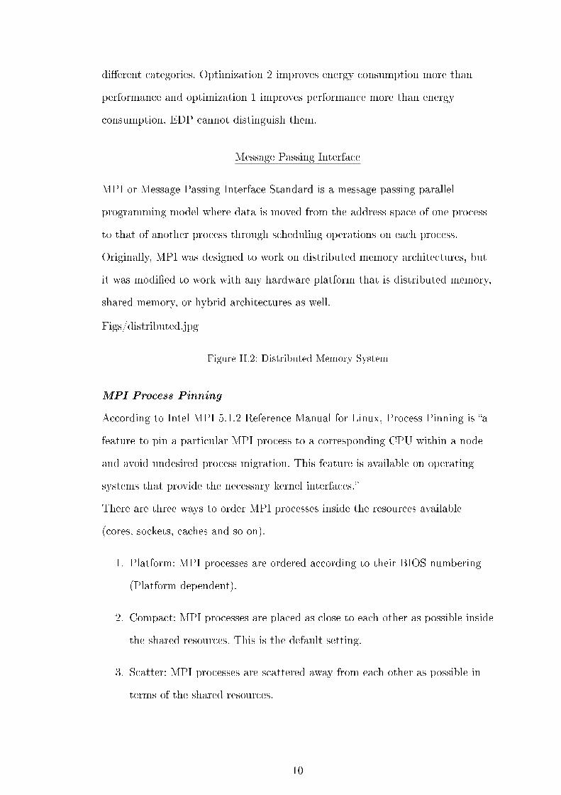
MPI or Message Passing Interface Standard is a message passing parallel

programming model where data is moved from the address space of one process

to that of another process through scheduling operations on each process.

Originally, MPI was designed to work on distributed memory architectures, but

it was modi�ed to work with any hardware platform that is distributed memory,

shared memory, or hybrid architectures as well.

Figs/distributed.jpg

Figure II.2: Distributed Memory System

MPI Process Pinning

According to Intel MPI 5.1.2 Reference Manual for Linux, Process Pinning is �a

feature to pin a particular MPI process to a corresponding CPU within a node

and avoid undesired process migration. This feature is available on operating

systems that provide the necessary kernel interfaces.�

There are three ways to order MPI processes inside the resources available

(cores, sockets, caches and so on).

1. Platform: MPI processes are ordered according to their BIOS numbering

(Platform dependent).

2. Compact: MPI processes are placed as close to each other as possible inside

the shared resources. This is the default setting.

3. Scatter: MPI processes are scattered away from each other as possible in

terms of the shared resources.

10

We used the compact default con�guration. For example, if number of cores is

24, this means that the �rst node will run 16 ranks and the second node will run

8 ranks. This way we can better study the power draw correlation to number of

ranks.

Machine Learning

As there exists a large number of MPI program con�gurations, many of which

seem correlated. It then becomes challenging to understand which set of

con�gurations should be used in order to obtain high performance and energy

e�ciency. Trying all the con�gurations can be a tedious and time consuming

task. So, we used machine learning models to help us estimate the performance

and the energy consumption of the program based on a smaller set of training

data. This is particularly important because it can predict the optimum number

of ranks to be used for MPI program.

In this section, the two learning models that have been used, and the reason for

choosing them among many other available models are discussed brie�y.

Linear and Nonlinear Regression

Regression is a statistical process of �nding relationship between data

variables.There are various models for regression. The models we used were

linear model and nonlinear model.

One of the uses of regression is to �t a curve or a surface to data points. This is

called curve �tting, which is a process of constructing a curve, or mathematical

function, that best �ts a series of dependent data points. We used Matlab Curve

Fitting Toolbox [4] to �nd the regression for our empirical data.

There are numerous �tting functions to data points. To name a few:

� First Degree Polynomial (Poly1):

y = p1x+ p2

11

� Second Degree Polynomial (Poly2):

y = p1x2 + p2x+ p3

� Third Degree Polynomial (Poly3):

y = p1x3 + p2x

2 + p3x+ p4

� Exponential (Exp):

y = p1ebx

� Smoothing Spline (SS): a spline is a numeric function that is

piecewise-de�ned by polynomial functions, and which possesses a high

degree of smoothness at the places where the polynomial pieces connect

(which are known as nodes). Smoothing spline divides the data points to

intervals and �ts each interval to a di�erent equation.

K-fold Cross Validation Technique

Cross-validation is a model assessment technique used to evaluate a machine

learning algorithm's performance in making predictions on new datasets that it

has not been trained on. It is done by partitioning a dataset into folds and using

a subset to train the algorithm and the remaining data for testing. Because

cross-validation does not use all of the data to build a model, it is a commonly

used method to prevent over�tting during training.

Each round of cross-validation involves randomly partitioning the original

dataset into a training set and a testing set. The training set is then used to

train a supervised learning algorithm and the testing set is used to evaluate its

performance. This process is repeated several times and the average

cross-validation error is used as a performance indicator.

The cross-validation technique we used is K-fold. It partitions data into K

randomly chosen subsets (or folds) of roughly equal size. One subset is used to

validate the model trained using the remaining subsets. This process is repeated

k times such that each subset is used exactly once for validation.

12

Doing curve �tting to empirical data inevitably introduces error. We calculated

two measures:

Root Mean Square Error

Root Mean Square Error (RMSE) is a common measure of the di�erences

between values predicted by a model or an estimator and the values actually

observed. RMSD represents sample standard deviation of the predicted from the

training data.

RMSE =

√ n∑i=1

(yprediction − ymeasured)2 (II.1)

R-Squared

R-squared is a number that ranges from 0 to 1 and shows the correlation

between a predicted value and training value. It is a statistic used in the context

of statistical models whose main purpose is either the prediction of future

outcomes or the testing of hypotheses, on the basis of other related information.

It provides a measure of how well observed outcomes are predicted by the model,

based on the proportion of total variation of outcomes explained by the model.

The larger the R-squared is, the more variability is explained by the linear

regression model.

R2 = 1−∑n

i=1 (yprediction − ymeasured)2∑n

i=1 y2measured

(II.2)

13

III. RELATED WORK

This section describes previous work on software energy e�ciency. We brie�y

present these works and compare it to our work.

Power Modeling Techniques

Many studies have researched how power is consumed on computer systems. One

study attempted to classify all models and metrics used to evaluate

energy-e�cient computer systems [5]. This study classi�ed current

energy-e�ciency metrics to three categories:

� Component-level Metrics that focuses on the processor level,

� System-level Metrics that focuses on the single-system level such as

performance per Watt, and

� Data Center-Level Metrics that various aspects of data center energy

e�ciency from the building's power and cooling provisioning to the

utilization of the computing equipment.

Our metrics can be classi�ed as component-level metrics that can be used to

compare two designs. To the best of our knowledge, the only comparable metric

to our research is the Energy Delay Product (EDP) [3], which is a fused metric

between energy and time delay. Unlike EDP, our metrics separate energy and

performance to provide more insights to the proposed optimization. Further

comparisons between the EDP metric and our proposed GPS-UP metrics can be

found in chapter VI.

At the system-level, metrics such as performance/Watt or SWaP (Space, Watt

and Performance) were proposed. Ge and Cameron [6] presented a power aware

speedup model for parallel systems. This model focuses on studying two aspects:

e�ect of changing number of nodes (parallelism), and processor frequency

14

(power). While these two aspects have major e�ect on speedup, the paper

neglects energy consumption. Moreover, Song et al. [7] developed the iso-energy

e�ciency model that accurately predicts total system energy consumption and

e�ciency for large scaling parallel systems. It tried to quantitatively understand

the e�ects of power and performance at scale. However, its method to predict

optimal system performance relied on EDP. EDP does not give the optimal

solution in certain cases. Also, their model evaluates machine and application

parameters. And our method evaluates code optimization e�ects.

We studied the impact of changing programming languages, compilers, and

implementations on software energy e�ciency[8]. We provided practical advice to

programmers on how to improve the energy e�ciency of their software. Recent

studies attempted to identify how researchers address software energy usage [9]

and how understudied that �eld is. In addition, researchers have investigated

software energy e�ciency among di�erent versions of code [10]. More studies

attempted to correlate temperature to source code [11].

Other studies present models of algorithm's energy consumption. For example,

Choi et al.[12] presented an algorithmic performance analysis of time, energy,

and power on HPC systems. However, the peak performances they were able to

achieve are hard to achieve on complicated algorithms. Awan and Petters [13]

studied the impact of race to halt on performance and energy e�ciency. Race to

halt is a strategy to make the algorithm run at top speed then shut down the

devices to save power. While this might be true in many cases, our methodology

proves that peak speedup does not imply peak greenup. By improving the code's

number of operations and the optimum usage of main memory and cache there is

more room for energy savings.

At the hardware level, cache recon�guration and DVFS has been studied

extensively. Totoni et al. [14] proposed a new technique to recon�gure the cache

adaptively using a runtime system that turns on/o� parts of cache according to

the cache utilization of the running software. In section VI, we will see that

15

DVFS falls in Category 4 and 6. Other literature studied the dark silicon [15]

[16], and proposed it as the future of hardware optimization after the

conventional scaling of CMOS technology has reached its limits.

Most of previous research in software optimization focused on improving

performance and maximizing speed. There is a common belief that a fast code

implies an energy e�cient code. In this thesis, we propose two new metrics,

greenup and powerup to measure software energy e�ciency. By observing the

relationship between these metrics, we were able to categorize software versions

and show that some optimization techniques can help energy more than

performance. We also pointed out the signi�cant improvement in energy

e�ciency for category 1 optimizations.

Power Measurement Tools

There are many computer power measurement techniques available. The energy

consumption of computer components can be obtained either via power models

or direct measurement. The idea of power modeling is to estimate the power

consumption of a node by correlating power with hardware performance counters

or other events. Two widely used CPU power models are Wattch [17] and

McPAT [18]. Direct measurement methods periodically pro�le the current and

voltage samples, calculate the power by multiplying the two values, and compute

the total energy as the integral of the power over the execution time. WattsUP

[19] is a famous power meter that can directly measure the total energy

consumed by an entire node. While WattsUP is easy to use but its sampling

frequency is very low (1 Hz). More importantly, it cannot pro�le power of

individual component(e.g. CPU or DRAM), which makes it insu�cient to

analyze the energy-e�ciency of complicated code. To tackle this problem, several

tools have been developed to provide detailed power consumption information.

PowerPack [20] is the most well-known tool, which was developed at Virginia

Tech for the power-aware cluster System G [21]. PowerPack measures the power

16

consumption of individual components (e.g., the CPU or DRAM) within a node.

However, its pro�ling approach is fairly expensive and hard to scale. It is worth

noting that built-in power sensors also gain popularity in accelerators and

co-processors. For example, GPUs such as Tesla C2075 and K20 and Intel Xeon

Phi both include onboard power sensors that allow direct power measurement

while a program is running [22].

Our power measurements are generated using the Marcher system [23]. The

Marcher system supports the development of a component-level power

measurement tool for major computer components. It is called pluggable Power

Data Acquisition Card (PODAC) for direct and decomposed power measurement.

We use a software tool that triggers the PODAC chips to measure power on the

execution hosts. We are mainly interested in CPU and DRAM power. All power

measurements are the sum of CPU and DRAM power.

Software Applications Analysis

Software energy e�ciency has been studied in many publications. Coplin and

Burtscher [24]studied the e�ect of software optimizations on runtime, energy and

power on 2 GPU applications. Not many studies addressed the power

consumption of MPI programs. Some papers studied the e�ect of using DVFS

with Large-Scale MPI Programs to save energy[25][26][27]. Liy et al. [28] studied

the e�ect of task aggregation (i.e., grouping multiple tasks within the same node

or the same multicore processor) on the power. They proposed a framework to

predict the e�ect of the task aggregation on runtime and energy. Other tools were

used to measure HPC (High Performance Computing) software performance such

as HPCToolkit [29] and MPI Performance Analysis Tool [30] and VAMPIR [31].

A comprehensive study was published by Muller et al. [32] that describes the

SPEC MPI 2007benchmark suite, and compare it with other benchmark suites.

Another study used scalasca Parallel performance analysis tool [33] to analyze

MPI 2007 benchmarks. The tool focuses on counting the number of MPI calls,

17

message size and other properties to �nd the execution behavior of the

applications. Also, there are many other productivity tools (debuggers,

performance counters, analyzers) for MPI, such as Marmot [34], PAPI [35] and

Periscope Tuning Framework[36].

18

IV. ALGORITHM DESCRIPTION

We selected six algorithms, Fast Fourier Transform (FFT), Towers of Hanoi,

Shellsort, Fibonacci series, Matrix Multiplication and Fractal. For each

algorithm, we have a number of di�erent implementations. The details of each

application are discussed below.

Fast Fourier Transform

A Fast Fourier Transform (FFT) is a fast algorithm to compute the Discrete

Fourier Transform (DFT) and its inverse. We implement FFT using the

Cooley-Tukey algorithm [37], which is a divide and conquer algorithm that

recursively breaks down a DFT of any composite size N = N1*N2 in terms of

smaller DFTs of sizes N1 and N2, consequently it reduces the computation time

to O(N log N) for highly-composite N. In our implementation, N must be a

power of 2. First, a �xed size array is allocated and initialized, then an in-place

N-point FFT is calculated. In C and C++, we use static arrays. In Java, the

array is assigned using the new operator. Note that all objects, including arrays,

are always allocated at run time in Java. We have identical C, C++, and Java

FFT implementations for two FFT algorithms. The �rst algorithm is recursive

FFT with twiddle factors computed at runtime. The second algorithm uses a

look-up table to precompute the twiddle factor and store them in memory, and

access them while running. We have 18 versions of FFT codes, and we executed

each code with 7 di�erent input sizes. Versions vary in programming languages

(C, C++, Java), algorithms (recursive calculation of twiddle factors v.s. look-up

table), compiler optimization �ags (-O1, -O2, -O3).

Towers Of Hanoi

Towers of Hanoi is a well-known mathematical game, which consists of three

rods and N number of disks of various sizes. The game starts with the disks

19

stacked so that their sizes are in ascending order on the �rst rod. The solution is

to move the disks to the third rod also in ascending order. There are two

conditions for moving the disks, to move one disk at a time, and to constantly

keep the disks in ascending order with respect to size. This algorithm

demonstrates the di�erence between a recursive algorithm and an iterative

algorithm in terms of energy consumption. To make a fair comparison, we have

an almost identical code. We started with Singh's 1998 implementation [38] and

generated code versions in C++ and Java for both iterative and recursive

implementation. We omitted C results as C++ have a nearly equal energy

consumption. We also added -O2 and -O3 optimization �ags to C++ and

omitted -O1 to reduce redundancy i.e. total of 8 versions.

Shellsort

Shellsort [39] is an in-place comparison-based sorting algorithm that has an

average time complexity of O(n3/2) and performs exceptionally well on

medium-to-large data sets. The algorithm works by comparing two elements that

are separated by a gap. The �rst element is compared to the element located gap

positions down the list, the next element is then located gap positions away, and

so on. Each new group of elements to be compared is assigned to a core. The

algorithm scales well because cores do not have data dependencies with each

other when comparing and swapping their sublists of elements. The algorithm is

computation intensive due to the compare and swap operations. The shellsort is

parallelized using OpenMP and the workload is distributed evenly.

Fibonacci

Fibonacci sequence [40] is a well-known math problem. The Fibonacci calculation

code that we measure calculates 45 Fibonacci numbers (i.e. Fib(2), Fib(3), ... ,

Fib (46)). Each Fibonacci calculation generates a task, which recursively

calculates the respective Fibonacci number of the sequence position. Each task is

20

assigned to a waiting thread to complete the actual computation of a Fibonacci

number. Since the work required to calculate large Fibonacci numbers (e.g. Fib

(46) and Fib (45)) is much heavier than small Fibonacci numbers (e.g. Fib(2)

and Fib(3)), this implementation has a skewed (i.e. highly unbalanced) workload.

Matrix Multiplication

Matrix multiplication was chosen because is it a widely used benchmark in

scienti�c computing. It is a C language MPI implementation. For these tests, two

randomly �lled 7,500 square matrices are multiplied together to yield a 7,500 x

7,500 matrix.

Fractal

Fractal [41] is a computationally intensive application requiring minimal memory

use. It is a C language MPI implementation. As implemented, the size is 40,320

by 40,320, with depth = 30. Fractal size is relatively large 40320 x 40320

unsigned chars = 1.5 GB.

21

V. POWER MEASUREMENT

Marcher System Con�guration

All experiments presented in this paper are executed on nodes of the Marcher

system, which is provided as part of the NSF funded Marcher project [23].

Marcher is a power-measurable heterogeneous cluster system containing

general-purpose multicores, GPU K20 accelerators and Intel Xeon Phi (MIC)

coprocessors, as well as DDR3 main memory and hybrid storage with hard drives

and SSDs. Marcher is equipped with complementary, easy to deploy

component-level power measurement tools for collecting accurate power

consumption data of all major components (e.g CPU, DRAM, Disk, GPU, and

Xeon Phi).

We used a cluster of 7 nodes on Marcher system.

Installed Packages:

� Sun Grid Engine.

� Intel Parallel Studio XE 2016.

� wget, csh, openssl-devel, compat-db, pam-devel and sshpass.

SGE issues Power measurement introduced error

System Speci�cations for each node is shown in Table V.1

MPI Power Measurement and Sun Grid Engine

To the best of our knowledge, there are no existing tools that can

accurately measure the energy consumption of a MPI program. There are

many performance counters but they do not measure power.

In order to measure power consumption of MPI applications, we had to

develop our own tools. The main challenge was to start the power meters

22

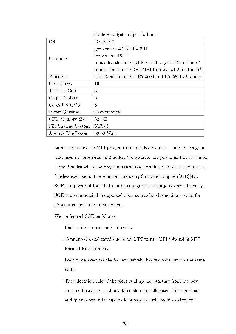
Table V.1: System Speci�cations

OS CentOS 7

Compiler

gcc version 4.8.3 20140911

icc version 16.0.1

mpicc for the Intel(R) MPI Library 5.1.2 for Linux*

mpiicc for the Intel(R) MPI Library 5.1.2 for Linux*

Processor Intel Xeon processor E5-2600 and E5-2600 v2 family

CPU Cores 16

Threads/Core 2

Chips Enabled 2

Cores Per Chip 8

Power Governor Performance

CPU Memory Size 32 GB

File Sharing System NFSv3

Average Idle Power 89.69 Watt

on all the nodes the MPI program runs on. For example, an MPI program

that uses 24 cores runs on 2 nodes. So, we need the power meters to run on

those 2 nodes when the program starts and terminate immediately after it

�nishes execution. The solution was using Sun Grid Engine (SGE)[42].

SGE is a powerful tool that can be con�gured to run jobs very e�ciently.

SGE is a commercially supported open-source batch-queuing system for

distributed resource management.

We con�gured SGE as follows:

� Each node can run only 16 ranks.

� Con�gured a dedicated queue for MPI to run MPI jobs using MPI

Parallel Environment.

� Each node executes the job exclusively. No two jobs run on the same

node.

� The allocation rule of the slots is �llup. i.e. starting from the best

suitable host/queue, all available slots are allocated. Further hosts

and queues are ��lled up� as long as a job still requires slots for

23

parallel tasks.

� Tight Integration of the MPICH2 library into SGE.

� Prolog Script: A startup shell script that runs before jobs to start the

power meters on the execution nodes.

� Epilog Script: A termination shell script that runs after jobs �nish to

kill the power meters on the execution nodes.

After successfully con�guring SGE to measure power of MPI programs. To

submit a code to a single node, we used this command:

qsub script.sh (V.1)

For multiple nodes, we used the following command, replacing <ranks>

with the desired number of MPI processes in integer form:

qsub -pe mpi <ranks> script.sh (V.2)

script.sh is a shell script that contains commands that we want to

measure its power consumption.

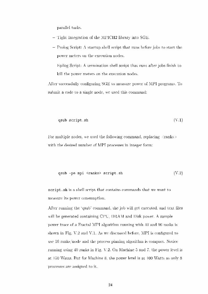
After running the `qsub' command, the job will get executed, and text �les

will be generated containing CPU, DRAM and Disk power. A sample

power trace of a Fractal MPI algorithm running with 40 and 96 ranks is

shown in Fig. V.2 and V.1. As we discussed before, MPI is con�gured to

use 16 ranks/node and the process pinning algorithm is compact. Notice

running using 40 ranks in Fig. V.2. On Machine 5 and 7, the power level is

at 150 Watts. But for Machine 8, the power level is at 100 Watts as only 8

processes are assigned to it.

24

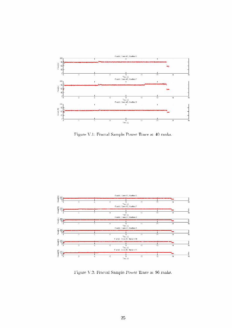
Figure V.1: Fractal Sample Power Trace at 40 ranks.

Figure V.2: Fractal Sample Power Trace at 96 ranks.

25

VI. THE GREENUP, POWERUP AND SPEEDUP METRICS

In Chapter II, we have illustrated the weakness of existing metrics (e.g.

total energy or EDP) in evaluating software energy e�ciency. In this

chapter, we propose the Greenup, Powerup and Speedup (GPS-UP in

short) metrics, which allow software developers intuitively understand the

correlations of performance, power, and energy for software optimizations.

The GPS-UP metrics are able to categorize almost all software

optimizations into one of the eight categories. We provide concrete

examples for optimizations that fall into each category. In addition, we

further discuss the advantages of GPS-UP over EDP with more examples.

It is worth noting that the GPS-UP metrics discussed in this chapter has

limitations in evaluating the energy e�ciency of software running on

multiple nodes (e.g. MPI programs), which will be addressed in the next

chapter.

GPS-UP metrics are 3 numbers calculated for each software run to evaluate

the relationship between energy, power and runtime. Depending on the

values of those 3 metrics, we can categorize the program optimization into

8 categories that covers all possible software optimizations.

Greenup, Powerup, and Speedup Metrics

The Speedup concept covers any comparison between two implementations

of the same algorithm whether it is a parallel or serial code. Assume we

have two implementations of an algorithm. One of them is an unoptimized

code (i.e. baseline code) and the other is an optimized code for better

performance or energy consumption. We de�ne the Speedup of the

optimized version as

26

Speedup =Tφ

To

, (VI.1)

where Tφ is the total execution time of non-optimized code, and To is the

total execution time of the optimized code. Similarly, we de�ne the term

Greenup as the ratio of the total energy consumption of the non-optimized

code (Eφ) over the total energy consumption of the optimized code (Eo).

Greenup is analogous to Speedup as it re�ects how green the optimized

code is in term of energy consumption.

Greenup =Eφ

Eo

, (VI.2)

Assuming, Pφ is the average power consumed by the non-optimized code

and Po is the average power consumed by the optimized code, we can

de�ne Eφ and Eo as

Eφ = TφPφ Eo = ToPo (VI.3)

By substituting Eq. VI.3 in Eq. VI.2, we get

Greenup =TφPφ

ToPo

=SpeedupPφ

Po

(VI.4)

We have de�ned Greenup and Speedup to measure the energy and

performance e�ects respectively. Eq. VI.4 introduces a new ratio to de�ne

27

the average power consumption ratio, namely Powerup.

Powerup =Po

Pφ

=Speedup

Greenup(VI.5)

Powerup implies the power e�ects of an optimization. A less than 1

Powerup implies power savings while a greater than 1 Powerup indicates

that the optimized code consumes more power in average. In Section VI,

Powerup is used with the Speedup together to categorize various software

optimizations in the GPS-UP Software Energy E�ciency Quadrant Graph

(See Fig. VI.1).

GPS-UP Software Categories

After we de�ned the Greenup, Powerup and Speedup metrics, we can

compare any two programs (or di�erent versions of the same program

provided that they complete the same the task) to �nd out which one is

better in terms of performance and energy e�ciency. Our method provides

a unique way to evaluate the impact of the optimized code on performance,

power and energy e�ciency by pinpointing it into one category of the

GPS-UP Software Energy E�ciency Quadrant Graph ( Fig. VI.1 illustrates

the eight GPS-UP software categories). Categories 1 - 4 are green categories

(i.e. saving energy) while categories 5 - 8 are red categories (i.e. consuming

more energy). More details about each category are discussed below.

Category 1

This green category is speci�ed as Powerup < 1, and Speedup > 1.

Category 1 optimizations run faster and consumes less power, leading to

more energy savings as both time and power have decreased. An example

of this category is discussed in chapter VI, which takes advantage of the

performance boost of relying more on the cache rather than CPU

28

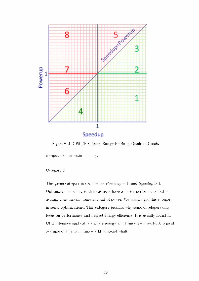
Figure VI.1: GPS-UP Software Energy E�ciency Quadrant Graph.

computation or main memory.

Category 2

This green category is speci�ed as Powerup = 1, and Speedup > 1.

Optimizations belong to this category have a better performance but on

average consume the same amount of power. We usually get this category

in serial optimizations. This category justi�es why some developers only

focus on performance and neglect energy e�ciency. It is usually found in

CPU intensive applications where energy and time scale linearly. A typical

example of this technique would be race-to-halt.

29

Category 3

This green category is speci�ed as Powerup > 1, Speedup > 1, and

Speedup > Powerup. Here, we achieved better performance at the expense

of consuming more power. Since the Speedup obtained is more than the

power penalty spent, the optimized code still saves energy. Category 2 and

3 are the most studied categories as they are easy to attain by doing simple

changes to the algorithm or the programming language. Most optimization

�ags in C and C++ language, plus some parallel algorithms fall into this

category.

Category 4

This green category is speci�ed as Powerup < 1, Speedup < 1, and

Speedup > Powerup. Here, we sacri�ce performance in favor of using less

power. Since the saved power is more than the performance degradation,

the optimized code still consumes less energy overall. Some DVFS

applications fall perfectly into this category.

Category 5

This red category is speci�ed as Powerup > 1, Speedup > 1, and

Powerup > Speedup. This is a controversial category, while current

literature might consider this as a better algorithm as the code runs faster.

In our method, we see this category as a red category because it consumes

more energy. The increase in Powerup is more than the improvement in the

Speedup. An example of this category would be the over-parallelization of

an algorithm, i.e. using an optimized parallel algorithm with a large

number of parallel devices that the energy overhead of the parallelization is

more than the gained performance.

30

Category 6

This red category is speci�ed as Powerup < 1, Speedup < 1, and

Speedup < Powerup. Optimizations belong to this category sacri�ce

performance in favor of using less power. But the power savings is not large

enough, leading to more energy consumption. Here, the sacri�ced

performance is larger than the power reduction thereby using more energy

than the base application. An example of this category is a DVFS code

implementation that uses a fairly low frequency. It consumes more energy

than its baseline version (Greenup < 1).

Category 7

This red category is speci�ed as Powerup = 1, Speedup < 1. We get worse

performance, and on average we did not save power. This optimization

implies that Speedup = Greenup and both of them are less than 1.

Category 8

This red category is speci�ed as Powerup > 1, Speedup < 1. It represents

worse performance, with more power consumption. This category shows

the worst case, an opposite of Category 1.

A Numerical Example

Now, it is time to further explain the proposed GPS-UP metrics and the

aforementioned categories using a concrete example. In Fig. ??, we

compare a C language recursive implementation of FFT at 2.6 GHz CPU

frequency, versus a C language recursive implementation with memoization

(Lookup table) of the twiddle factors and -O1 �ag at 1.2 GHz CPU

frequency. The base version calculates 9,961,472 double twiddle factors.

31

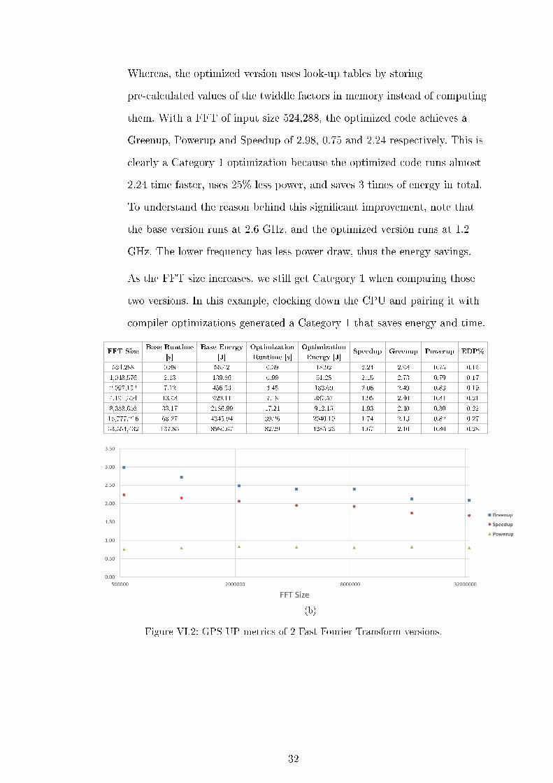
Whereas, the optimized version uses look-up tables by storing

pre-calculated values of the twiddle factors in memory instead of computing

them. With a FFT of input size 524,288, the optimized code achieves a

Greenup, Powerup and Speedup of 2.98, 0.75 and 2.24 respectively. This is

clearly a Category 1 optimization because the optimized code runs almost

2.24 time faster, uses 25% less power, and saves 3 times of energy in total.

To understand the reason behind this signi�cant improvement, note that

the base version runs at 2.6 GHz, and the optimized version runs at 1.2

GHz. The lower frequency has less power draw, thus the energy savings.

As the FFT size increases, we still get Category 1 when comparing those

two versions. In this example, clocking down the CPU and pairing it with

compiler optimizations generated a Category 1 that saves energy and time.

FFT SizeBase Runtime

[s]

Base Energy

[J]

Optimization

Runtime [s]

Optimization

Energy [J]Speedup Greenup Powerup EDP%

524,288 0.88 56.42 0.39 18.92 2.24 2.98 0.75 0.15

1,048,576 2.13 139.86 0.99 51.28 2.15 2.73 0.79 0.17

2,097,152 7.12 456.53 3.45 183.69 2.06 2.49 0.83 0.19

4,194,304 13.98 929.11 7.18 387.57 1.95 2.40 0.81 0.21

8,388,608 33.17 2186.99 17.21 912.15 1.93 2.40 0.80 0.22

16,777,216 68.27 4345.94 39.26 2040.10 1.74 2.13 0.82 0.27

33,554,432 137.83 8980.67 82.29 4285.26 1.67 2.10 0.80 0.28

(b)

Figure VI.2: GPS-UP metrics of 2 Fast Fourier Transform versions.

32

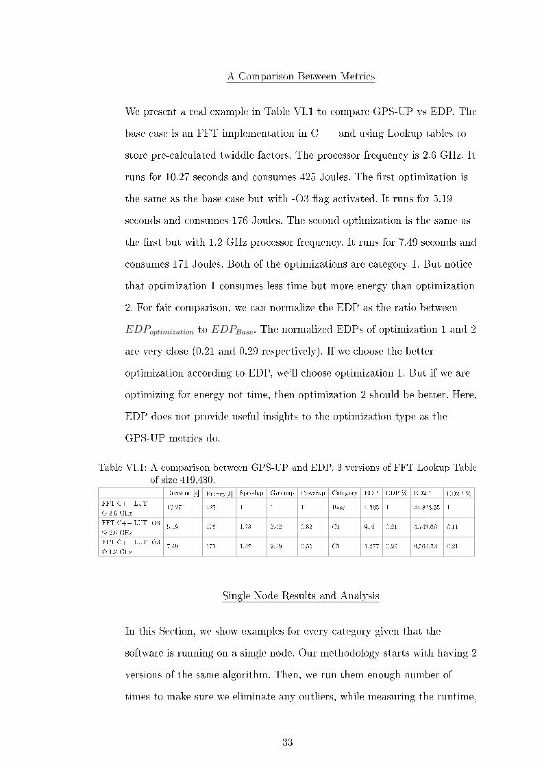
A Comparison Between Metrics

We present a real example in Table VI.1 to compare GPS-UP vs EDP. The

base case is an FFT implementation in C++ and using Lookup tables to

store pre-calculated twiddle factors. The processor frequency is 2.6 GHz. It

runs for 10.27 seconds and consumes 425 Joules. The �rst optimization is

the same as the base case but with -O3 �ag activated. It runs for 5.19

seconds and consumes 176 Joules. The second optimization is the same as

the �rst but with 1.2 GHz processor frequency. It runs for 7.49 seconds and

consumes 171 Joules. Both of the optimizations are category 1. But notice

that optimization 1 consumes less time but more energy than optimization

2. For fair comparison, we can normalize the EDP as the ratio between

EDPoptimization to EDPBase. The normalized EDPs of optimization 1 and 2

are very close (0.21 and 0.29 respectively). If we choose the better

optimization according to EDP, we'll choose optimization 1. But if we are

optimizing for energy not time, then optimization 2 should be better. Here,

EDP does not provide useful insights to the optimization type as the

GPS-UP metrics do.

Table VI.1: A comparison between GPS-UP and EDP. 3 versions of FFT Lookup Table

of size 419,430.Runtime [s] Energy[J] Speedup Greenup Powerup Category EDP EDP % ED2P ED2P %

FFT C++ LUT

@ 2.6 GHz10.27 425 1 1 1 Base 4,365 1 44,828.55 1

FFT C++ LUT -O3

@ 2.6 GHz5.19 176 1.98 2.42 0.82 C1 914 0.21 4,743.66 0.11

FFT C++ LUT -O3

@ 1.2 GHz7.49 171 1.37 2.49 0.55 C1 1,277 0.29 9,564.73 0.21

Single Node Results and Analysis

In this Section, we show examples for every category given that the

software is running on a single node. Our methodology starts with having 2

versions of the same algorithm. Then, we run them enough number of

times to make sure we eliminate any outliers, while measuring the runtime,

33

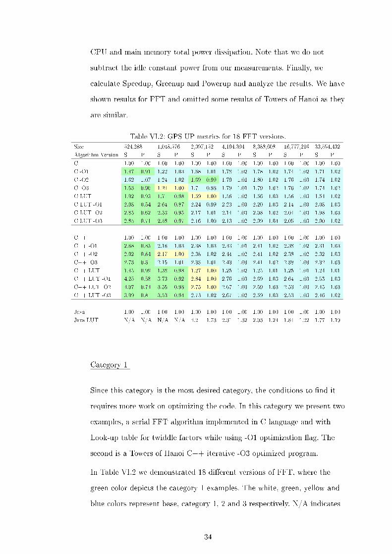
CPU and main memory total power dissipation. Note that we do not

subtract the idle constant power from our measurements. Finally, we

calculate Speedup, Greenup and Powerup and analyze the results. We have

shown results for FFT and omitted some results of Towers of Hanoi as they

are similar.

Table VI.2: GPS-UP metrics for 18 FFT versions.

Size 524,288 1,048,576 2,097,152 4,194,304 8,388,608 16,777,216 33,554,432

Algorithm Version S P S P S P S P S P S P S P

C 1.00 1.00 1.00 1.00 1.00 1.00 1.00 1.00 1.00 1.00 1.00 1.00 1.00 1.00

C -O1 1.47 0.91 1.22 1.03 1.68 1.01 1.78 1.02 1.78 1.02 1.74 1.02 1.71 1.02

C -O2 1.62 1.07 1.24 1.02 1.69 0.99 1.79 1.01 1.80 1.02 1.76 1.03 1.74 1.02

C -O3 1.53 0.96 1.24 1.00 1.7 0.98 1.79 1.01 1.79 1.02 1.76 1.02 1.74 1.02

C LUT 1.92 0.93 1.7 0.98 1.59 1.00 1.56 1.02 1.56 1.03 1.56 1.03 1.54 1.02

C LUT -O1 2.98 0.54 2.64 0.87 2.24 0.99 2.23 1.03 2.20 1.03 2.14 1.03 2.08 1.03

C LUT -O2 2.85 0.62 2.53 0.95 2.17 1.01 2.14 1.03 2.08 1.02 2.04 1.03 1.98 1.03

C LUT -O3 2.85 0.71 2.58 0.97 2.16 1.00 2.13 1.02 2.09 1.04 2.05 1.03 2.00 1.02

C++ 1.00 1.00 1.00 1.00 1.00 1.00 1.00 1.00 1.00 1.00 1.00 1.00 1.00 1.00

C++ -O1 2.68 0.85 2.16 1.03 2.38 1.03 2.43 1.01 2.41 1.02 2.38 1.02 2.31 1.03

C++ -O2 2.92 0.84 2.17 1.00 2.38 1.02 2.44 1.02 2.41 1.02 2.38 1.02 2.32 1.03

C++ -O3 2.73 0.8 2.15 1.01 2.38 1.01 2.43 1.03 2.41 1.02 2.38 1.03 2.32 1.03

C++ LUT 1.45 0.99 1.38 0.98 1.27 1.00 1.25 1.02 1.25 1.01 1.25 1.01 1.24 1.01

C++ LUT -O1 4.25 0.58 3.73 0.92 2.84 1.00 2.76 1.03 2.69 1.03 2.64 1.03 2.53 1.03

C++ LUT -O2 4.07 0.74 3.55 0.98 2.75 1.00 2.67 1.03 2.59 1.03 2.53 1.03 2.45 1.03

C++ LUT -O3 3.99 0.8 3.53 0.94 2.73 1.02 2.67 1.02 2.59 1.03 2.53 1.03 2.46 1.02

Java 1.00 1.00 1.00 1.00 1.00 1.00 1.00 1.00 1.00 1.00 1.00 1.00 1.00 1.00

Java LUT N/A N/A N/A N/A 4.2 1.73 2.31 1.32 2.03 1.24 1.84 1.22 1.77 1.19

Category 1

Since this category is the most desired category, the conditions to �nd it

requires more work on optimizing the code. In this category we present two

examples, a serial FFT algorithm implemented in C language and with

Look-up table for twiddle factors while using -O1 optimization �ag. The

second is a Towers of Hanoi C++ iterative -O3 optimized program.

In Table VI.2 we demonstrated 18 di�erent versions of FFT, where the

green color depicts the category 1 examples. The white, green, yellow and

blue colors represent base, category 1, 2 and 3 respectively. N/A indicates

34

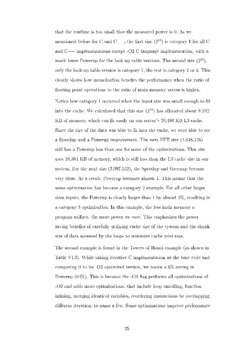
that the runtime is too small that the measured power is 0. As we

mentioned before for C and C++, the �rst size (219) is category 1 for all C

and C++ implementations except -O2 C language implementation, with a

much lower Powerup for the look-up table versions. The second size (220),

only the look-up table version is category 1, the rest is category 2 or 3. This

clearly shows how memoization bene�ts the performance when the ratio of

�oating point operations to the ratio of main memory access is higher.

Notice how category 1 occurred when the input size was small enough to �t

into the cache. We calculated that this size (219) has allocated about 8,192

KB of memory, which can �t easily on our server's 20,480 KB L3 cache.

Since the size of the data was able to �t into the cache, we were able to see

a Speedup and a Powerup improvement. The next FFT size (1,048,576)

still has a Powerup less than one for some of the optimizations. This size

uses 16,384 KB of memory, which is still less than the L3 cache size in our

system. For the next size (2,097,152), the Speedup and Greenup become

very close. As a result, Powerup becomes almost 1. This means that the

same optimization has become a category 2 example. For all other larger

sizes inputs, the Powerup is clearly larger than 1 by almost 3%, resulting in

a category 3 optimization. In this example, the less main memory a

program utilizes, the more power we save. This emphasizes the power

saving bene�ts of carefully utilizing cache size of the system and the chunk

size of data accessed by the loops to minimize cache miss rate.

The second example is found in the Towers of Hanoi example (as shown in

Table VI.3). While taking iterative C implementation as the base code and

comparing it to its -O3 optimized version, we notice a 6% saving in

Powerup (94%). This is because the -O3 �ag performs all optimizations of

-O2 and adds more optimizations, that include loop unrolling, function

inlining, merging identical variables, reordering instructions by overlapping

di�erent iteration, to name a few. Some optimizations improve performance

35

and some don't. Therefore, it is recommended to try all the optimization

�ags and see which one performs better. Although, this optimization is

category 1, still the best optimization is the recursive with -O3 �ag.

Table VI.3: GPS-UP metrics of Towers of Hanoi (N = 28 discs).

Algorithm

Version

Runtime

[s]

Total

Energy [J]Speedup Greenup Powerup Category

C++

Iterative25.92 1280.49 1.00 1.00 1.00 Base

C++

Iterative -O22.30 113.51 11.27 11.28 1.00 C2

C++

Iterative -O32.29 106.51 11.35 12.02 0.94 C1

C++

Recursive2.50 124.91 10.25 10.25 1.00 C2

C++

Recursive -O21.23 71.67 21.08 17.87 1.18 C3

C++

Recursive -O31.21 62.18 21.42 20.59 1.04 C3

Java

Iterative88.68 4901.44 0.29 0.26 1.12 C8

Java Recursive 1.26 114.95 20.55 11.14 1.84 C3

Table VI.4: GPS-UP metrics for Shellsort.

Input

Size

S G P S G P S G P S G P S G P S G P

1 Core 2 Cores 4 Cores 8 Cores 16 Cores 32 Cores

500000 1.00 1.00 1.00 1.70 1.45 1.18 2.92 2.13 1.37 4.70 2.75 1.71 6.03 2.95 2.05 2.53 0.95 2.65

1000000 1.00 1.00 1.00 1.72 1.57 1.09 2.98 2.44 1.22 4.82 3.06 1.57 6.66 2.28 2.91 4.01 1.14 3.52

Category 2

The example of this category would be an optimization that runs faster

without a signi�cant change in power consumption (i.e. powerup is equal to

1). In Table VI.2, seven category 2 examples (coloured in yellow) are found

in the transition between the input size that �ts in the cache (220) and the

input size that is larger than cache (221). This means that the base

program and its optimization consume the same average instantaneous

power, which can be referred to the fact that FFT is a CPU intensive

application, where the relation between time and energy is linear. When

36

the input size becomes too large, this ratio starts to increase due to

increased memory usage.

Another example of category 2 is found in the towers of Hanoi application

in Table VI.3, which is also a CPU intensive application. The three

examples are C++ iterative with -O2 �ag, C++ recursive, and Java

recursive. The main observation is that the Java code runs faster than the

C++ versions. The Greenup is 11.4 compared to the C++ iterative

version. This indicates that the Java Virtual Machine's (JVM) energy cost

is minimal thanks to optimizations and code predictions in JVM. One such

optimization that is used in our Towers of Hanoi implementation is

Just-in-time (JIT) compilation in the JVM. Sunâs JVM combines both

interpretation of byte code and JIT compilation. The Java byte code is

initially interpreted, and if portions of the code are being frequently

executed, the JVM compile these portions to native code. In our algorithm,

the recursive version clearly outlines repetitive code that the JVM detects

and compiles to native code at runtime (JIT compilation)[43].

Category 3

This is the most common category to occur in software optimization. The

program runs faster but the Powerup also increases. We will demonstrate

two examples: a serial examples (FFT versions) and a parallel example

(Shellsort OpenMP versions). In Table VI.2 the Powerup might increase

from 2-3% like the di�erent C and C++ implementations, or increase from

19-73% like in Java Look-up Table versions.

In the Java Look-up Table version, the Speedup does not remain constant

like in the C version. On the contrary, the larger the input size, the less

Speedup we obtain. This is a well-known issue when scaling the size of Java

applications.The larger the input size becomes, the deeper in category 3 it

37

gets with larger Powerup and less Speedup.

Table VI.4 presents 10 versions of the Shellsort parallel implementation.

While taking the 1 core implementation as the base, we computed the

GPS-UP metrics for 2, 4, 8, 16, 32. As the number of utilized cores

increases, more power is consumed and hence Powerup increases. Most

parallel applications are category 3 optimization because they improve

performance and consume more power due to the increased power

consumption of using more cores. Note that the processor in our compute

node only has 16 cores. Therefore, running at 32 cores activates

hyper-threading, which explains the decrease in Speedup and Greenup and

the increase in Powerup compared to the 16 cores version. In this example,

hyper-threading does not improve energy e�ciency.

Category 4

In this category, we run our FFT code while reducing the maximum

processor frequency from 2.6 GHz to 1.2 GHz. This CPU frequency scaling

is a form of Dynamic Voltage Frequency Scaling (DVFS) that hurts

performance but the program runs with less energy consumption than the

energy used in the higher frequency. Note that category 4 is considered a

green category as it saves energy, on the contrary to category 6 which hurts

performance and uses more energy. In Table VI.5, the only category 4

optimization is the three C++ optimized versions, where the Speedup is

larger than the Powerup. This shows that C++ optimization �ags are more

e�cient than C optimization �ags.

By observing the FFT C++ implementation with -O3 �ag in Table VI.5,

the EDP for the base case at 2.6 GHz is 120,249. While the EDP for the

1.2 GHz is 178,129. The normalized EDP of the 1.2 GHz version compared

to the 2,6 GHz version is 1.48. It is well known that larger EDP means

38

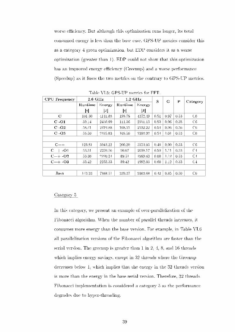
worse e�ciency. But although this optimization runs longer, its total

consumed energy is less than the base case. GPS-UP metrics consider this

as a category 4 green optimization, but EDP considers it as a worse

optimization (greater than 1). EDP could not show that this optimization

has an improved energy e�ciency (Greenup) and a worse performance

(Speedup) as it fuses the two metrics on the contrary to GPS-UP metrics.

Table VI.5: GPS-UP metrics for FFT.

CPU Frequency 2.6 GHz 1.2 GHzS G P Category

Runtime

[s]

Energy

[J]

Runtime

[s]

Energy

[J]

C 101.30 4141.88 198.78 4272.49 0.51 0.97 0.53 C6

C -O1 59.14 2450.99 111.56 2551.13 0.53 0.96 0.55 C6

C -O2 58.41 2419.88 108.51 2532.22 0.54 0.96 0.56 C6

C -O3 58.50 2425.83 108.50 2392.92 0.54 1.01 0.53 C6

C++ 123.81 5043.22 260.20 5573.05 0.48 0.90 0.53 C6

C++ -O1 53.51 2259.56 90.07 2030.17 0.59 1.11 0.53 C4

C++ -O2 53.36 2220.34 89.51 1989.63 0.60 1.12 0.53 C4

C++ -O3 53.42 2233.53 89.42 1992.05 0.60 1.12 0.53 C4

Java 143.33 7888.51 339.27 9303.68 0.42 0.85 0.50 C6

Category 5

In this category, we present an example of over-parallelization of the

Fibonacci algorithm. When the number of parallel threads increases, it

consumes more energy than the base version. For example, in Table VI.6

all parallelization versions of the Fibonacci algorithm are faster than the

serial version. The greenup is greater than 1 in 2, 4, 8, and 16 threads

which implies energy savings, except in 32 threads where the Greenup

decreases below 1, which implies that the energy in the 32 threads version

is more than the energy in the base serial version. Therefore, 32 threads

Fibonacci implementation is considered a category 5 as the performance

degrades due to hyper-threading.

39

Table VI.6: GPS-UP metrics of Fibonacci OpenMP.

No. of

Threads

Runtime

[s]

Total

Energy[J]S G P Category

1 43.01 2708 1.00 1.00 1.00 Base

2 19.17 1589 2.24 1.70 1.32 C3

4 12.75 1332 3.37 2.03 1.66 C3

8 13.16 1590 3.27 1.70 1.92 C3

16 14.60 2187 2.95 1.24 2.38 C3

32 20.58 3310 2.09 0.82 2.55 C5

Category 6

The most common example of this category is DVFS with a fairly low

frequency. In Table VI.5, all the versions are category 6 except C++ -O1,

-O2, and -O3 which are category 4. Powerup is larger than Speedup. In

those versions the program runs slower but consumes more energy than the

base version at 2.6 GHz. Therefore, this category is considered energy

ine�cient. Judging this category by runtime only will not give us the

overall picture of how much energy was saved. Using the GPS-UP metrics

helped to distinguish between the green category 4 and the red category 6.

Category 7 and 8

These two red categories are found when the optimization degrades

performance while having a Greenup which is equal to or less than the

Speedup. Category 7 and 8 are the direct opposite of category 2 and 1

respectively. One example of category 8 is found in Table VI.3 where

iterative Java implementation of the algorithm is slower and more energy

consuming than its C++ iterative version. This shows clearly how the

choice of programming language a�ects both speedup and greenup of the

code. Native code used in C and C++ is usually much faster to compile

than byte code that runs on a virtual machine such as Java or OCaml.

40

We demonstrated 2 Category 1 examples in FFT and Towers of Hanoi

algorithms. Also, we found Category 2 and 3 in FFT. OpenMP Shellsort

demonstrated Category 3 and 5. DVFS examples of Category 4 and 6 were

found when we use a lower CPU frequency in FFT. Categories 7 and 8

were found in Java implementation when compared to C++.

41

VII. EXTENDING GPS-UP METRICS FOR MPI

PROGRAMS

Modeling MPI Programs

MPI has become the de facto standard for communication for parallel

programs running on a distributed memory system. In the previous

chapter, we discussed how to use GPS-UP metrics to evaluate the energy

e�ciency of software running on a single node. However, the previous

metrics are not su�cient in evaluating software running on multiple nodes

(e.g. MPI programs). This is primarily because servers in a cluster usually

are not turned o� (even when no jobs are running), which leads to a

constant idle power (a parameter that cannot be ignored). If we use the

previously de�ned GPS-UP metrics, there will be no power savings (i.e.

green category) for all MPI programs. This is because the power increases

linearly with the number of nodes but the speedup cannot keep up with a

linear growth (close to linear in the best scenario). But in order to evaluate

performance on a distributed system, we need to consider more factors.

Therefore, in this chapter, we extend the GPS-UP metrics to make it

applicable to MPI programs (or any programs that run on multiple nodes).

Speedup calculation method is the same. But we had to modify Greenup

equation to account for multiple nodes. Our initial approach to calculate

Greenup was to sum the DRAM and CPU energy for each node the

program runs on. While increasing the number of CPUs n, Greenup scaled

very rapidly resulting in category 5 or 8 for all optimizations. But MPI is

widely used and it saves energy. So, for multiple node software, we

rede�ned Greenup to include idle power. To measure GPS-UP metrics on a

distributed system, we need to de�ne some parameters:

42

� N : Total number of nodes in the cluster

� n : Number of nodes on which the MPI program runs.

� ranks : Number of CPU ranks (cores) on which the MPI program

runs.

� Eia : Active energy of MPI program execution on node i.

� Pi : Average power of an idle node.

� Tφ : The execution time of a MPI program when running on a single

node.

� Eφ : The energy consumption of a MPI program when running on a

single node. Assuming all cores in the node has been fully utilized.

� To : The execution time of a MPI program when running on n nodes.

� Eo : The energy consumption of a MPI program when running on n

nodes.

Energy consumption for MPI execution on n nodes is:

Eo =n∑

x=1

Exa +

N∑y=n+1

P yi To (VII.1)

Assuming that the cluster nodes are identical,∑N

y=n+1 Pyi can be

approximated to (N − n).Pi. The new equation becomes:

Eo =n∑

x=1

Exa + (N − n)PiTo (VII.2)

A realistic way to calculate energy is to add the idle power of nodes that

are not contributing any work to the program execution. Since these nodes

are already consuming energy. This way the energy cost of adding a new

node will not largely decrease Greenup. The notion behind this is that data

43

centers already pay the electric bill for all of their nodes even the idle ones.

So, executing the program using more nodes will utilize the massive

computational power of a large cluster and might save overall energy.

Let's take the base case to be program execution on 1 node, assuming full

core utilization. Greenup for MPI execution on n nodes is:

Greenup =Eφ

Eo

=E1

o + (N − 1)PiTφ∑ni=1E

ia + (N − n)PiTo

(VII.3)

Speedup and Powerup are calculated using their regular equations VI.1 and

VI.5. Moreover, we measured idle power Pi on over 80 nodes at di�erent

times and concluded that the average idle power for our system is 89.69

Watts.

Predicting Energy and Runtime of MPI programs

Despite the fact that MPI programs have been used for decades, choosing

the optimal number of ranks (for best performance) for a given MPI

program still largely depends on programmers' experiences and their

familiarities with the system hardware and con�gurations. Very few work

has discussed the power issues of MPI programs.

Simply choosing the best Speedup can waste a lot of energy. Also, �nding

this optimal number of cores can take a multiple trial and error attempts.

Therefore, we used curve �tting to predict energy and runtime of the

program execution. Then to asses the predicted model, we used K-fold

cross validation.

In the next section, we conducted some experiments using matrix

multiplication. Then, we measured the runtime and energy consumption

while changing the number of cores n. These runs were used as a training

data to �nd the curve equation.

44

Multiple Node Results and Analysis

In this section, we present MM and Fractal GPS-UP metrics and

prediction model.

Matrix Multiplication GPS-UP metrics

A trend shows in MPI results, there is a certain number of ranks for each

algorithm after which the performance starts to decline. In MPI software,

the more ranks we use the more communication overhead due to dividing

up the work and collecting the results back. We need to �nd the perfect

number of ranks that bene�ts from parallelization but does not increase

communication overhead until it becomes an issue. Our research focuses on

�nding that perfect spot.

Table VII.1 shows the results of MM. We vary the number of ranks in each

run. The base version is the 8 ranks. All the optimized versions are

Category 3. This algorithm scales well until 88 ranks, the best speedup is

8.59. Then Speedup starts to decline.

It is clear that speedup scales well with number of ranks. Also, Greenup

scales from 1 at ranks = 8 to 5.64 at ranks = 88. Then t starts to

decrease. This is an interesting number because this means that although

we used 7 nodes to run our program, the energy we consumed has been

reduced. This shows the signi�cance of idle power and that it is a high

contributor to wasted energy. Also, including idle power while measuring

Greenup has alleviated the e�ect of using more ranks.

As for Powerup, it scales almost linearly with number of cores. Every time

we add a new machine (multiples of 16 ranks) the Powerup is increased by

almost 10% until it reaches 1.7 at 112 ranks. This is an expected result, as

112/16 = 7. So, the increase in Powerup is 70% at 112 ranks. Moreover,

45

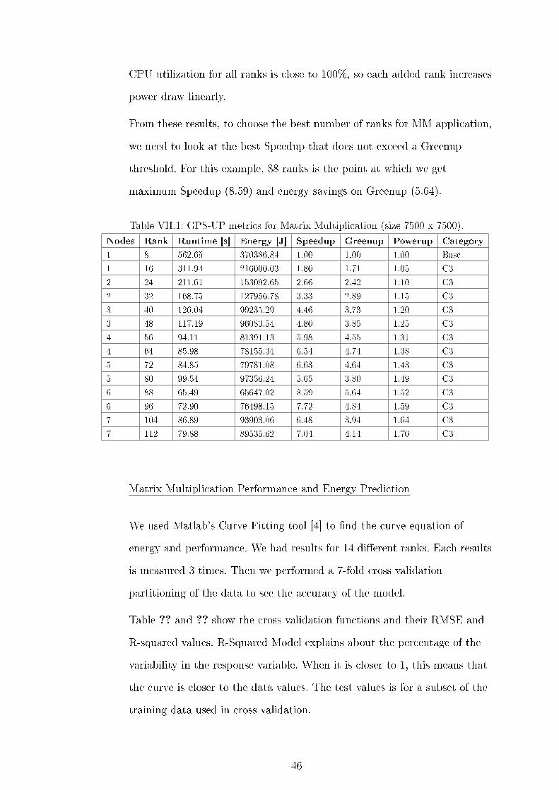
CPU utilization for all ranks is close to 100%, so each added rank increases

power draw linearly.

From these results, to choose the best number of ranks for MM application,

we need to look at the best Speedup that does not exceed a Greenup

threshold. For this example, 88 ranks is the point at which we get

maximum Speedup (8.59) and energy savings on Greenup (5.64).

Table VII.1: GPS-UP metrics for Matrix Multiplication (size 7500 x 7500).

Nodes Rank Runtime [s] Energy [J] Speedup Greenup Powerup Category

1 8 562.65 370386.84 1.00 1.00 1.00 Base

1 16 311.94 216000.03 1.80 1.71 1.05 C3

2 24 211.61 153092.65 2.66 2.42 1.10 C3

2 32 168.75 127956.78 3.33 2.89 1.15 C3

3 40 126.04 99235.29 4.46 3.73 1.20 C3

3 48 117.19 96083.54 4.80 3.85 1.25 C3

4 56 94.11 81391.13 5.98 4.55 1.31 C3

4 64 85.98 78155.34 6.54 4.74 1.38 C3

5 72 84.85 79781.08 6.63 4.64 1.43 C3

5 80 99.54 97356.24 5.65 3.80 1.49 C3

6 88 65.49 65647.02 8.59 5.64 1.52 C3

6 96 72.90 76498.15 7.72 4.84 1.59 C3

7 104 86.89 93903.06 6.48 3.94 1.64 C3

7 112 79.88 89535.62 7.04 4.14 1.70 C3

Matrix Multiplication Performance and Energy Prediction

We used Matlab's Curve Fitting tool [4] to �nd the curve equation of

energy and performance. We had results for 14 di�erent ranks. Each results

is measured 3 times. Then we performed a 7-fold cross validation

partitioning of the data to see the accuracy of the model.

Table ?? and ?? show the cross validation functions and their RMSE and

R-squared values. R-Squared Model explains about the percentage of the

variability in the response variable. When it is closer to 1, this means that

the curve is closer to the data values. The test values is for a subset of the

training data used in cross validation.

46

In Fig. ??, we compared di�erent curve equations. For Time model, we

notice that smoothing spline has the lowest RMSE and highest R-Squared

making it the best �t. The second best is the 3rd order polynomial. We will

select the poly3 to avoid over �tting of the curve. Over�tting is a problem

that occurs during training. Although the error for the curve is driven to a

very small value, when new data is added to the test set the error becomes

very large. The poly3 linear model is:

To(n) = p1.n3 + p2.n2 + p3.n+ p4 (VII.4)

Coe�cients (with 95% con�dence bounds):

p1 = −0.001724(−0.002142,−0.001306)

p2 = 0.3882(0.3121, 0.4643)

p3 = −27.62(−31.62,−23.62)

p4 = 705.8(648.3, 763.2)

Function RMSE-TEST RMSE-TRAIN Rsquared-TEST Rsquared-TRAIN

SS 17.35 17.52 0.99 0.99

poly1 92.67 92.70 0.51 0.51

poly2 56.79 56.93 0.82 0.82

poly3 34.19 34.25 0.94 0.94

exp1 58.25 58.34 0.81 0.81

(a)

(b)

Figure VII.1: MM Time Prediction Model and Error.

47

In Fig. ??, we compared di�erent curve equations. For Active Energy

model, again smoothing spline has the lowest RMSE and highest

R-Squared making it the best �t. The second best is the third order

polynomial. While smoothing spline has the best results, we will select the

poly2 to avoid over �tting of the curve. The poly2 linear model is:

Eo(n) = p1.n2 + p2.n+ p3 (VII.5)

Coe�cients (with 95% con�dence bounds):

p1 = 6.559(2.184, 10.93)

p2 = 32.05(−507.6, 571.7)

p3 = 59100(45020, 73180)

Function RMSE-TEST RMSE-TRAIN Rsquared-TEST Rsquared-TRAIN

SS 9683.01 9720.74 0.92 0.92

poly1 14222.54 14200.96 0.78 0.78

poly2 12976.66 12937.13 0.83 0.83

poly3 13039.43 12978.79 0.83 0.83

exp1 13103.94 13088.69 0.82 0.82

(a)

(b)

Figure VII.2: MM Energy Prediction Model and Error.

48

Fractal GPS-UP metrics

Fractal is di�erent from MM. When we measured its performance, we

found that total runtime does not scale well. So, to �nd the reason for this

we used mpiP MPI pro�ling tool [44]. The tool showed that the �nal stage

of the program MPI_Gather call was throttling the performance. Since

Fractal size is relatively large (40320 x 40320 unsigned chars = 1.5 GB), it

is expected for this algorithm not not scale well. The communication cost

is very high that it outweighs any parallelization bene�t.

We calculated the average time of each rank except for rank 0 which runs

the MPI_Gather call. Then, we compared it to the total wallclock time in

table VII.2. Althought, ranks �nish their computations relatively quickly.

They remain in a busy waiting state until MPI_Gather call �nishes.

Table VII.3 shows the GPS-UP metrics of Fractal. We vary the number of

ranks in each run. The base version is the 8 ranks. The optimized versions

are Category 3 except at 96 and 112 ranks. They are Category 5. Speedup

does not scale linearly, and Greenup values degrades with more ranks. We

demonstrated this example to show an example where using more ranks

improves performance slightly but ends up consuming more energy than

the 1 node base version. As for Powerup, it also scales almost linearly with

number of cores like MM.

From these results, to choose the best number of ranks for MPI fractal

application, the best Speedup is at 16 ranks, i.e. 1 node.

Fractal Performance and Energy Prediction

We had results for 12 di�erent ranks. Each results is measured 15 times.

Using resgession, we obtained the curve equation of energy and

performance. Then we performed a 7-fold cross validation partitioning of

the data to see the accuracy of the model.

49

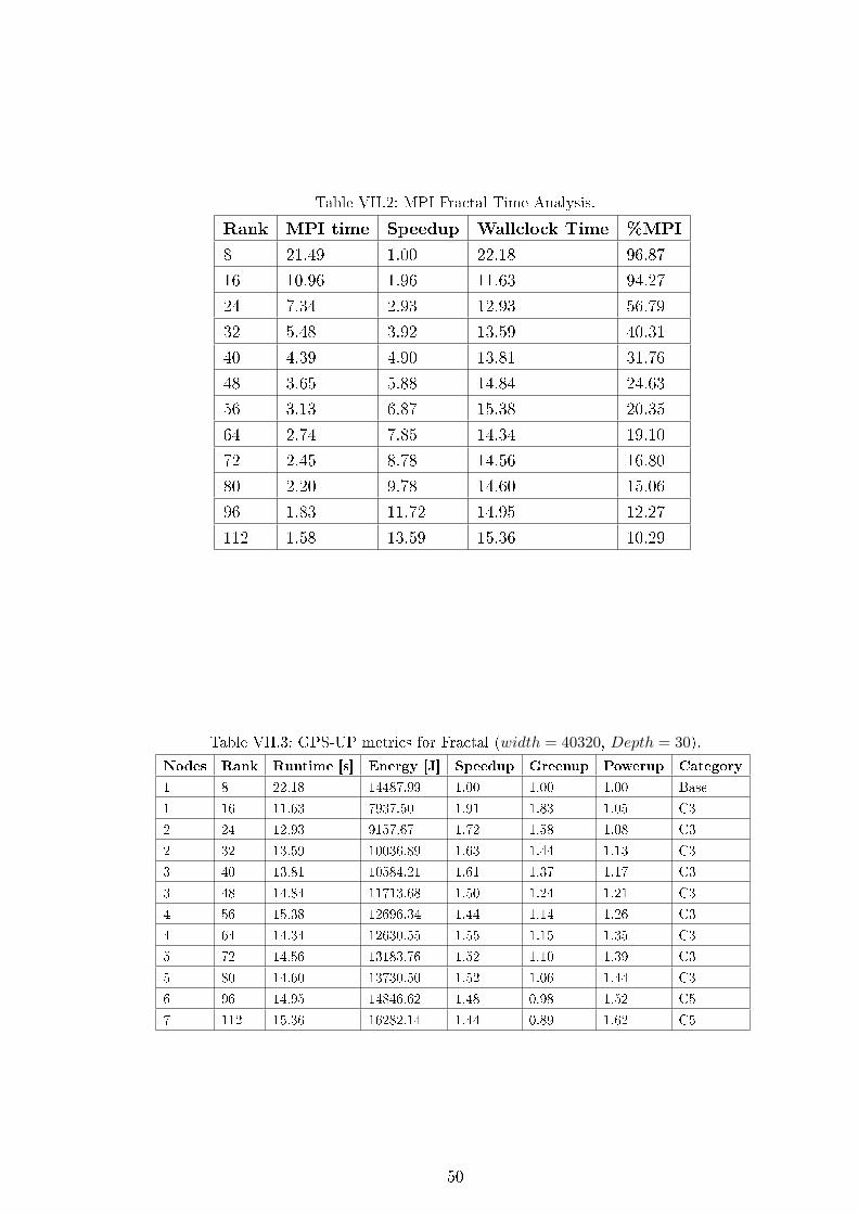
Table VII.2: MPI Fractal Time Analysis.

Rank MPI time Speedup Wallclock Time %MPI

8 21.49 1.00 22.18 96.87

16 10.96 1.96 11.63 94.27

24 7.34 2.93 12.93 56.79

32 5.48 3.92 13.59 40.31

40 4.39 4.90 13.81 31.76

48 3.65 5.88 14.84 24.63

56 3.13 6.87 15.38 20.35

64 2.74 7.85 14.34 19.10

72 2.45 8.78 14.56 16.80

80 2.20 9.78 14.60 15.06

96 1.83 11.72 14.95 12.27

112 1.58 13.59 15.36 10.29

Table VII.3: GPS-UP metrics for Fractal (width = 40320, Depth = 30).

Nodes Rank Runtime [s] Energy [J] Speedup Greenup Powerup Category

1 8 22.18 14487.99 1.00 1.00 1.00 Base

1 16 11.63 7937.50 1.91 1.83 1.05 C3

2 24 12.93 9157.67 1.72 1.58 1.08 C3

2 32 13.59 10036.89 1.63 1.44 1.13 C3

3 40 13.81 10584.21 1.61 1.37 1.17 C3

3 48 14.84 11713.68 1.50 1.24 1.21 C3

4 56 15.38 12696.34 1.44 1.14 1.26 C3

4 64 14.34 12630.55 1.55 1.15 1.35 C3

5 72 14.56 13183.76 1.52 1.10 1.39 C3

5 80 14.60 13730.50 1.52 1.06 1.44 C3

6 96 14.95 14846.62 1.48 0.98 1.52 C5

7 112 15.36 16282.14 1.44 0.89 1.62 C5

50

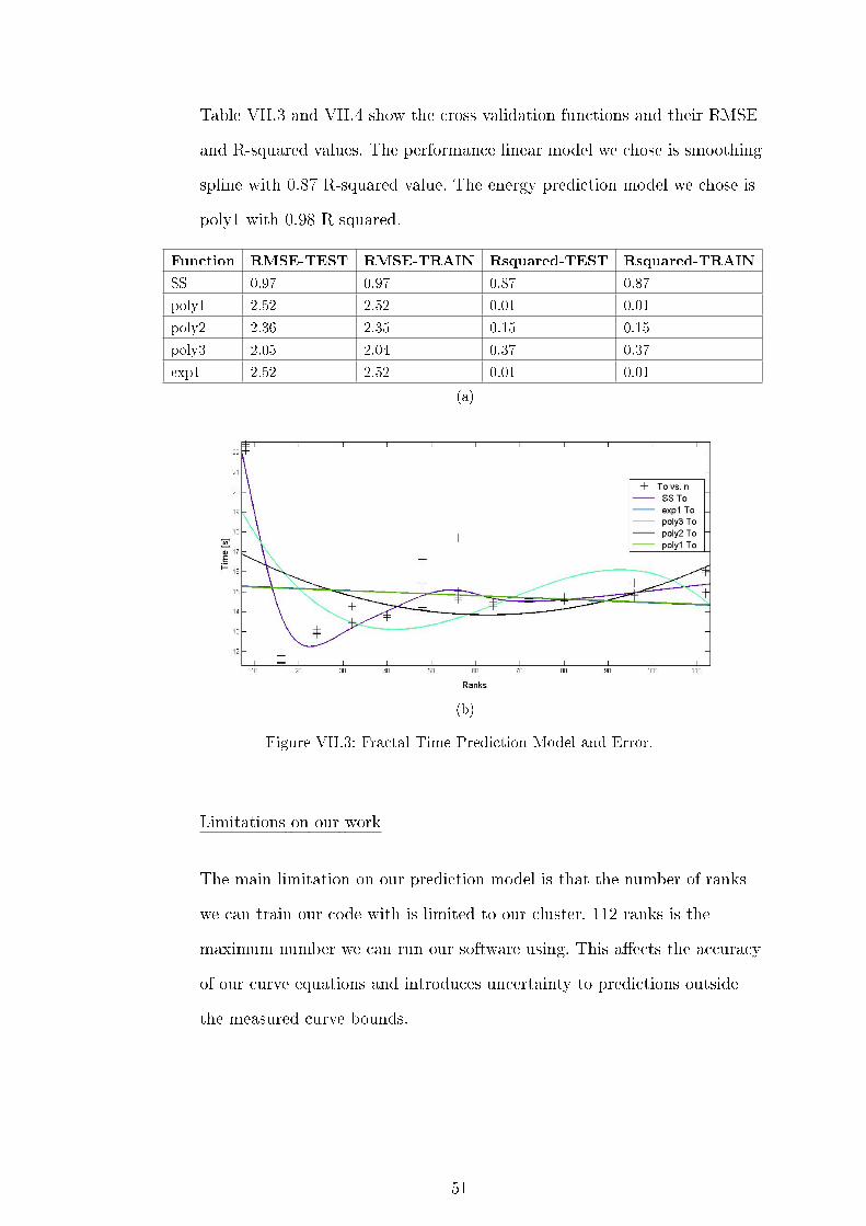
Table VII.3 and VII.4 show the cross validation functions and their RMSE

and R-squared values. The performance linear model we chose is smoothing

spline with 0.87 R-squared value. The energy prediction model we chose is

poly1 with 0.98 R-squared.

Function RMSE-TEST RMSE-TRAIN Rsquared-TEST Rsquared-TRAIN

SS 0.97 0.97 0.87 0.87

poly1 2.52 2.52 0.01 0.01

poly2 2.36 2.35 0.15 0.15

poly3 2.05 2.04 0.37 0.37

exp1 2.52 2.52 0.01 0.01

(a)

(b)

Figure VII.3: Fractal Time Prediction Model and Error.

Limitations on our work

The main limitation on our prediction model is that the number of ranks

we can train our code with is limited to our cluster. 112 ranks is the

maximum number we can run our software using. This a�ects the accuracy

of our curve equations and introduces uncertainty to predictions outside

the measured curve bounds.

51

Function RMSE-TEST RMSE-TRAIN Rsquared-TEST Rsquared-TRAIN

SS 387.32 386.91 0.99 0.99

poly1 607.57 606.85 0.98 0.98

poly2 570.15 569.22 0.98 0.98

poly3 537.46 536.49 0.99 0.99

exp1 1073.71 1071.62 0.94 0.94

(a)

(b)

Figure VII.4: Fractal Energy Prediction Model and Error.

52

VIII. CONCLUSION

This section summarizes the contributions and work done in this thesis,

and provides recommendations for work in the future.

Contribution

This thesis proposes using the Greenup, Powerup and Speedup (GPS-UP)

metrics to systematically study the performance and energy e�ciency of

serial and parallel programs. We use six selected parallel algorithms to

demonstrate the impact of hardware and compiler choice, algorithm design

and optimization, running code with di�erent programming languages,

altering the algorithm, using DVFS, changing compiler optimizations and

changing the number of ranks in MPI programs.

The GPS-UP metrics are able to demonstrate the di�erences between

optimizations. We found category 1, 2 and 3 optimizations in FFT

algorithm, category 3 and 5 in MM and Fractal MPI implementations, and

category 4 and 6 in FFT DVFS optimizations. The GPS-UP metrics

enables us to use a simple yet comprehensive way to evaluate the impact of

various types of software (even hardware) optimizations on the

performance and energy e�ciency of diverse programs.

In MPI software applications, we rede�ned Greenup metric to include

cluster idle energy. This enabled us to see the potential energy savings MPI

applications can provide. We demonstrated that some MPI applications

performance scale with number of ranks until it reaches a turning point at

which performance degrades. Other applications performance does not

scale well, so using a large number of ranks will be a waste of energy.

We used curve �tting to predict runtime and active energy of MM and

Fractal MPI algorithms. To verify our model, we used K-fold

53

cross-validation partitioning to see the accuracy of the model. MM model

was highly accurate (R-squared = 0.91), but Fractal performance

prediction model was not accurate, as the training runtime values were

almost constant. This is due to the high communication cost that

outweighed the parallelization cost.

Future Work

Our future work involves expanding the prediction model and use a large

number of algorithms as training data. Also, it is possible to add more

variables to the model and expand the GPS-UP metrics as needed.

54

REFERENCES

[1] E. Capra, C. Francalanci, and S. A. Slaughter, �Green IT: MeasuringApplication Software Energy E�ciency,� IT Professional, vol. 14,pp. 54�61, March 2012.

[2] B. Steigwald, C. D. Lucero, C. Akella, and A. R. Agrawal, EnergyAware Computing: Powerful Approaches for System Design. IntelPress, 2011.

[3] R. Gonzalez and M. Horowitz, �Energy dissipation in general purposemicroprocessors,� vol. 31 of 9, IEEE Journal Of Solid-State Circuits,September 1996.

[4] �Matlab Curve Fitting Tools.�http://www.mathworks.com/products/curvefitting/. Accessed:06-03-2016.

[5] S. Rivoire, Models and Metrics for Energy-E�cient Computer

Systems. PhD thesis, 2008.

[6] R. Ge and K. W. Cameron, �Power-aware speedup,� Parallel andDistributed Processing Symposium (IPDPS), IEEE International,March 2007.

[7] S. Song, C. Su, R. Ge, and K. W. Cameron, �Iso energy e�ciency: Anapproach to power-constrained parallel computation,� Parallel &Distributed Processing Symposium (IPDPS), IEEE International,March 2011.

[8] S. Abdulsalam, D. Lakomski, Q. Gu, T. D. Jin, and Z. L. Zong,�Program energy e�ciency: The impact of language, compiler andimplementation choices,� IEEE International Conference on GreenComputing (IGCC'14), November 2014.

[9] G. Pinto, F. Castor, and Y. D. Liu, �Mining questions about softwareenergy consumption,� pp. 22�31, 11th Working Conference on MiningSoftware Repositories (MSR 2014), 2014.

[10] A. Hindle, �Green mining: A methodology of relating software changeto power consumption,� pp. 78�87, Mining Software Repositories(MSR 2012), 9th IEEE Working Conference, June 2012.

[11] K. W. Cameron, H. K. Pyla, and S. Varadarajan, �Tempest: Aportable tool to identify hot spots in parallel code,� InternationalConference on Parallel Processing (ICPP), September 2007.

[12] J. Choi, M. Dukhan, X. Liu, and R. W. Vuduc, �Algorithmic time,energy, and power on candidate hpc compute building blocks,� In 8thIEEE International Parallel & Distributed Processing Symposium(IPDPS), May 2014.

55

[13] M. A. Awan and S. M. Petters, �Race-to-halt energy savingstrategies,� Journal of Systems Architecture, October 2014.

[14] E. Totoni, J. Torrellas, and L. V. Kale, �Using an adaptive hpcruntime system to recon�gure the cache hierarchy,� pp. 1047�1058,International Conference for High Performance Computing,Networking, Storage and Analysis (SC'14), November 2014.

[15] N. Goulding-Hotta et al., �The greendroid mobile applicationprocessor: An architecture for silicon's dark future,� vol. 31 of 2,pp. 86 �95, IEEE Micro, March 2011.

[16] M. B. Taylor, �A landscape of the new dark silicon design regime,�vol. 33 of 5, pp. 8�19, IEEE Micro, August 2013.

[17] D. Brooks et al., �Wattch: A framework for architectural-levelpoweranalysis and optimizations,� pp. 83�94, ACM/IEEEInternational Symposium on Computer Architecture, June 2000.

[18] S. Li, J. Ahn, R. Strong, J. Brockman, D. Tullsen, and N. Jouppi,�Mcpat: An integrated power, area, and timing modeling frameworkfor multicore and manycore architectures,� pp. 469�480, IEEE/ACMInternational Symposium on Microarchitecture, 2009.

[19] �Watts up Meter.� http://www.wattsupmeters.com. Accessed:06-03-2016.

[20] R. Ge, X. Z. Feng, S. Song, H. Chang, D. Li, and K. Cameron,�Powerpack: Energy pro�ling and analysis of high-performancesystems and applications,� vol. 21 of 5, pp. 658�671, IEEETransactions on Parallel and Distributed Systems, 2010.

[21] �System G.� http://www.cs.vt.edu/node/4666. Accessed:06-03-2016.

[22] M. Burtscher, I. Zecena, and Z. L. Zong, �Measuring GPU Power withthe K20 Built-in Sensor,� GPGPU'07, 2014.

[23] �Marcher NSF award.�http://nsf.gov/awardsearch/showAward?AWD_ID=1305359.Accessed: 06-03-2016.

[24] J. Coplin and M. Burtscher, �E�ects of source-code optimizations ongpu performance and energy consumption,� pp. 48�58, GPGPU-8Proceedings of the 8th Workshop on General Purpose Processingusing GPUs, 2015.

[25] B. Rountree, D. Lowenthal, S. Funk, V. Freeh, B. de Supinski, andM. Schulz, �Bounding Energy Consumption in Large-scale MPIprograms,� pp. 1�9, Supercomputing. Proceedings of the 2007ACM/IEEE Conference, November 2007.

56

[26] V. Freeh, F. Pan, N. Kappiah, D. Lowenthal, and R. Springer,�Exploring the energy-time tradeo� in mpi programs on apower-scalable cluster,� p. 4.1, IPDPS '05 Proceedings of the 19thIEEE International Parallel and Distributed Processing Symposium,2005.

[27] A. Guermouche, N. Triquenaux, B. Pradelle, and W. Jalby,�Minimizing energy consumption of mpi programs in realisticenvironment,� Research Report - Universite de VersaillesSaint-Quentin-en-Yvelines., 2015.

[28] D. Liy, D. Nikolopoulosz, K. Camerony, B. de Supinski, andM. Schulz, �Power-aware MPI task aggregation prediction for highendcomputing systems,� pp. 1�12, Parallel Distributed Processing(IPDPS), 2010 IEEE International Symposium, April 2010.

[29] �HPCToolkit.� http://hpctoolkit.org/. Accessed: 06-03-2016.

[30] �MPI Performance Analysis Tools.�http://nci.org.au/user-support/for-developers/

mpi-performance-analysis-tools/. Accessed: 06-03-2016.

[31] W. Nagel, A. Arnold, M. Weber, H. Hoppe, and K. Solchenbach,�VAMPIR: Visualization and Analysis of MPI Resources,�Supercomputer, vol. 12, pp. 69�80, 1996.

[32] M. Muller, M. Waveren, R. Lieberman, B. Whitney, H. Saito,K. Kumaran, J. Baron, W. Brantley, C. Parrott, T. Elken, H. Feng,and C. Ponder10, �SPEC MPI2007: an application benchmark suitefor parallel systems using mpi,� vol. 22, pp. 191�205, June 2012.

[33] Z. Szebenyi, B. Wylie, and F. Wolf, �SCALASCA parallel performanceanalyses of SPEC MPI2007 applications,� vol. 5119, pp. 99�123, 2008.

[34] B. Krammer, T. Hilbrich, V. Himmler, B. Czink, K. Dichev, andM. Muller, Tools for High Performance Computing. Springer BerlinHeidelberg, 2011.

[35] V. Weaver, M. Johnson, K. Kasichayanula, J. Ralph, P. Luszczek,D. Terpstra, and S. Moore, �Measuring Energy and Power withPAPI,� Parallel Processing Workshops (ICPPW), August 2012.

[36] �Periscope Tuning Framework.�http://periscope.in.tum.de/?page_id=62. Accessed: 06-03-2016.

[37] �FFT.� http://rosettacode.org/wiki/Fast_Fourier_transform.Accessed: 06-03-2016.

[38] �Towers of hanoi.�http://www.kernelthread.com/projects/hanoi/. Accessed:06-03-2016.

57

[39] �Shellsort.� http://en.wikipedia.org/wiki/Shellsort. Accessed:06-03-2016.

[40] �Fibonacci series.� http://en.wikipedia.org/wiki/Fibonacci.Accessed: 06-03-2016.

[41] �Fractal MPI.� CS 5351 - Parallel Processing. Matrin Burtscher.

[42] �Sun Grid Engine.� http://gridscheduler.sourceforge.net/.Accessed: 06-03-2016.

[43] A. Noureddine, Towards a Better Understanding of the Energy

Consumption of Software Systems. PhD thesis, 2014.

[44] �mpiP MPI Pro�ling.� http://mpip.sourceforge.net/. Accessed:06-03-2016.

58