using stochastic differential equations for wind and solar...

Using stochastic differential equations for windand solar power forecasting

Henrik Madsen, Emil Banning Iversen,Peder Bacher, Jan Kloppenborg Møller

Department of Applied Mathematics and Computer Science, DTU

eSACP Project Meeting, DTU

October 5, 2017

Outline

Introduction

Probabilistic Forecasting

Stochastic Differential Equations in Forecasting

Example: A Probabilistic Model for Wind Power

Example: Spatio-Temporal Model for Solar Power

Using Probabilistic Forecasts

Conclusion

Motivation

An Energy System with a Large Renewable Component

source: http://www.imm.dtu.dk/ jbjo/smartenergy.html

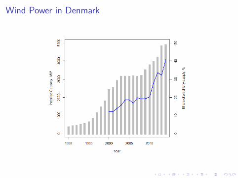
Wind Power in Denmark

Renewable Energy and Uncertainty

Challenges with Renewable EnergyI Wind, solar and wave energy depend on the weather system.I The weather is inherently uncertain, implying thatI Wind, wave and solar energy is intermittent and uncertain.I This uncertainty affects the supply and demand for energy, the

energy infrastructure and the economics of the energy system.

Overcoming the ChallengesI Understanding the uncertainty associated with renewable

energy becomes valuable.I Input knowledge of uncertainty into decision problems.I Solve decision problems for minimizing the issues related to

this uncertainty.

Renewable Energy and Uncertainty

Challenges with Renewable EnergyI Wind, solar and wave energy depend on the weather system.I The weather is inherently uncertain, implying thatI Wind, wave and solar energy is intermittent and uncertain.I This uncertainty affects the supply and demand for energy, the

energy infrastructure and the economics of the energy system.

Overcoming the ChallengesI Understanding the uncertainty associated with renewable

energy becomes valuable.I Input knowledge of uncertainty into decision problems.I Solve decision problems for minimizing the issues related to

this uncertainty.

Topics related to eSACP

AimsI To produce probabilistic forecasts quantifying this uncertainty.I To consider applications of such probabilistic forecasts.

ApproachesI Modeling uncertainty using:

I Stochastic differential equationsI Stochastic partial differential equations

I Applying optimization tools incorporating uncertainty:I Stochastic Programming based on scenarios for future states)

Topics related to eSACP

AimsI To produce probabilistic forecasts quantifying this uncertainty.I To consider applications of such probabilistic forecasts.

ApproachesI Modeling uncertainty using:

I Stochastic differential equationsI Stochastic partial differential equations

I Applying optimization tools incorporating uncertainty:I Stochastic Programming based on scenarios for future states)

Probabilistic Forecasting

What is Probabilistic ForecastingPoint Forecast

I Focus on describing typical or most likely outcome.I A single value point value for each point in time.

Probabilistic ForecastI Describes (features of) the predictive distribution.I Probabilistic if it makes use of probabilities in the forecast.I Examples of probabilistic forecasts include:

I Quantile forecastsI Prediction intervalsI Predictive densitiesI Scenarios

I These options are used in some state-of-the-art tools for windpower forecasting (WPPT) and solar power forecasting(SolarFor)For more information we refer to https://www.enfor.dk)

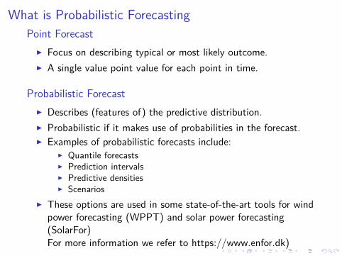
What is Probabilistic ForecastingPoint Forecast

I Focus on describing typical or most likely outcome.I A single value point value for each point in time.

Probabilistic ForecastI Describes (features of) the predictive distribution.I Probabilistic if it makes use of probabilities in the forecast.I Examples of probabilistic forecasts include:

I Quantile forecastsI Prediction intervalsI Predictive densitiesI Scenarios

I These options are used in some state-of-the-art tools for windpower forecasting (WPPT) and solar power forecasting(SolarFor)For more information we refer to https://www.enfor.dk)

Stochastic DifferentialEquations in Forecasting

The Basic SetupThe basic stochastic differential equation formulation:

Xt = X0 +∫ t

0f (Xs , s)ds +

0g(Xs , s, )dWs ,

We use the short-hand interpretation of this integral equation:

dXt = f (Xt , t)dt + g(Xt , t)dWt

Yk = h(Xtk , tk , ek).

The predictive density, j(x , t), can be found by solving (withg(Xt , t) =

√2D(Xt , t)):

∂t j(x , t) = − ∂

∂x [f (x , t)j(x , t)] + ∂2

∂x2 [D(x , t)j(x , t)] . (1)

Xt = X0 +∫ t

0f (Xs , s)ds +

0g(Xs , s, )dWs ,

√2D(Xt , t)):

∂t j(x , t) = − ∂

∂x [f (x , t)j(x , t)] + ∂2

∂x2 [D(x , t)j(x , t)] . (1)

Xt = X0 +∫ t

0f (Xs , s)ds +

0g(Xs , s, )dWs ,

√2D(Xt , t)):

∂t j(x , t) = − ∂

∂x [f (x , t)j(x , t)] + ∂2

∂x2 [D(x , t)j(x , t)] . (1)

Example: A ProbabilisticModel for Wind Power

The Data

I The Klim Fjordholme wind farm with a rated capacity of 21MW.

I Hourly measurements for three years.I Numerical weather predictions from Danish Meteorological

Institute, updated every 6 hours.

A SDE Model

Wind dynamics given by:

dXt =((

1− e−Xt)

(ρx pt + Rt) + θx (ptµx − Xt))

dt + σxX 0.5t dWx ,t

dRt = −θr Rtdt + σr dWr ,t

Y1,k = Xtk + ε1,k

Wind to power dynamics given by:

dQt = (St − θqQt)dt + σqdWq,t

dSt = −θsStdt + σsdWs,t

Y2,k = (0.5 + 0.5 tanh(5(Xtk − γ1))) (0.5− 0.5 tanh(γ2(Xtk − γ3)))ζ3

1 + e−ζ1(Xtk −ζ2+Qtk ) + ε2,k

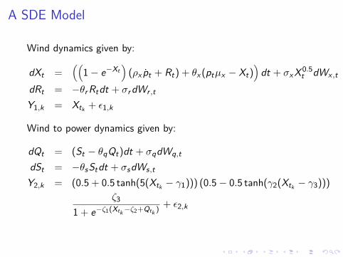
A SDE Model

Wind dynamics given by:

dXt =((

1− e−Xt)

(ρx pt + Rt) + θx (ptµx − Xt))

dt + σxX 0.5t dWx ,t

dRt = −θr Rtdt + σr dWr ,t

Y1,k = Xtk + ε1,k

Wind to power dynamics given by:

dQt = (St − θqQt)dt + σqdWq,t

dSt = −θsStdt + σsdWs,t

Y2,k = (0.5 + 0.5 tanh(5(Xtk − γ1))) (0.5− 0.5 tanh(γ2(Xtk − γ3)))ζ3

1 + e−ζ1(Xtk −ζ2+Qtk ) + ε2,k

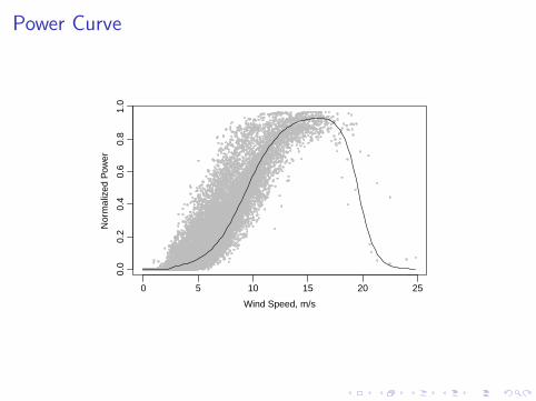
Power Curve

0 5 10 15 20 25

Wind Speed, m/s

Multi-Horizon Probabilistic Forecasts

Predictive density of production in percent out of rated power forthe Klim wind farm:

Model Performance 1-step-ahead

Model performance on 1-hour ahead predictions on test set:

Test Set

Models Parameters MAE RMSE CRPS

Climatology - 0.2208 0.2693 0.1417Persistence 1 0.0509 0.0835 0.0428AR 4 0.0527 0.0820 0.0417ARX 5 0.0510 0.0795 0.0406ARX - TN 7 0.0648 0.0848 0.0444ARX - GARCH 9 0.0505 0.0797 0.0382ARX - GARCH - TN 11 0.0575 0.0823 0.0401Model 19 0.0471 0.0773 0.0327

Model Performance on Multiple Horizons

Model multi-horizons predictions performance on test set:

Models CRPS for different horizons Energy Score

1 hour 4 hours 12 hours 24 hours

ARX - GARCH 0.0382 0.0704 0.0787 0.0789 1.180ARX - GARCH - TN- iterative

0.0401 0.0783 0.1043 0.1225 1.945

Model 0.0327 0.0641 0.0779 0.0836 0.739

Example: A Spatio-TemporalForecast Model for Solar Power

The Data

I A solar power plant with a nominal output of 151 MW.I Measurements of 91 inverters every second for one year.I We consider a cutout of 5 by 14 inverters for modeling.

Motivation

ChallengesI A high dimensional problem, with 70 inverters and forecast

horizon of two miutes.I Classical methods are have a large high dimensional parameter

space.I As a result typically a large computational burden.

ApproachI A model that incorporates the physics of the system.I Good local models should lead to good global models.I A physical understanding of the system leads to fewer

parameters and lowered computational burden.

Motivation

ChallengesI A high dimensional problem, with 70 inverters and forecast

horizon of two miutes.I Classical methods are have a large high dimensional parameter

space.I As a result typically a large computational burden.

ApproachI A model that incorporates the physics of the system.I Good local models should lead to good global models.I A physical understanding of the system leads to fewer

parameters and lowered computational burden.

The Framework

We propose a model of the form:

dUi ,j,t = f (Ui ,j,t , t) dt + g(Ui ,j,t , t)dWi ,j,t (2)Yl ,k = h(Utk , tk) + εl ,k , (3)

where Ui ,j,t = {Ui ,j,t ,Ui−1,j,t ,Ui+1,j,t ,Ui ,j−1,t ,Ui ,j+1,t}.

Ui,j,t

Ui−1,j,t Ui+1,j,t

Ui−1,j+1,t Ui,j+1,t Ui+1,j+1,t

Ui−1,j−1,t Ui,j−1,t Ui+1,j−1,t

The Framework

We propose a model of the form:

dUi ,j,t = f (Ui ,j,t , t) dt + g(Ui ,j,t , t)dWi ,j,t (2)Yl ,k = h(Utk , tk) + εl ,k , (3)

where Ui ,j,t = {Ui ,j,t ,Ui−1,j,t ,Ui+1,j,t ,Ui ,j−1,t ,Ui ,j+1,t}.

Ui,j,t

Ui−1,j,t Ui+1,j,t

Ui−1,j+1,t Ui,j+1,t Ui+1,j+1,t

Ui−1,j−1,t Ui,j−1,t Ui+1,j−1,t

SPDE Model

Stochastic Partial Differential EquationI Normalize the parameters with the spatial distance in

appropriate way.I Parameters become grid-invariant.I Can be interpreted as a stochastic partial differential equation.

The dynamical model interpretation:

dU(x , t) = vθ∇U(x , t)dt + σdW (x , t),

with the deterministic part dU(x , t) = vθ∇U(x , t)dt being auni-directional wave equation.

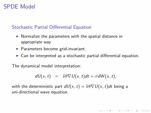
SPDE Model

Stochastic Partial Differential EquationI Normalize the parameters with the spatial distance in

appropriate way.I Parameters become grid-invariant.I Can be interpreted as a stochastic partial differential equation.

The dynamical model interpretation:

dU(x , t) = vθ∇U(x , t)dt + σdW (x , t),

with the deterministic part dU(x , t) = vθ∇U(x , t)dt being auni-directional wave equation.

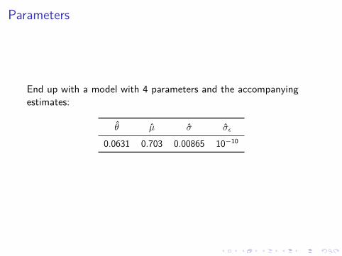
Parameters

End up with a model with 4 parameters and the accompanyingestimates:

θ µ σ σε

0.0631 0.703 0.00865 10−10

Predicting Spatio-Temporal Power Output

Power production in percent out of rated power.

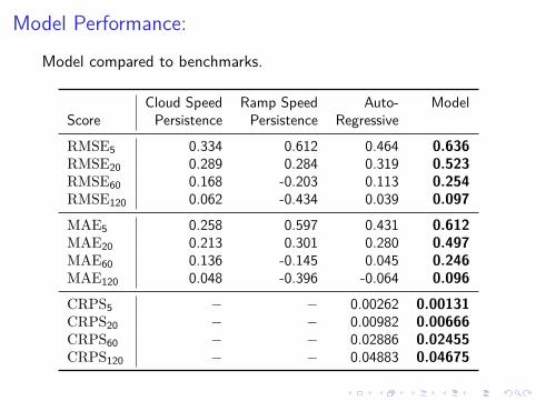
Model Performance:Model compared to benchmarks.

Cloud Speed Ramp Speed Auto- ModelScore Persistence Persistence Regressive

RMSE5 0.334 0.612 0.464 0.636RMSE20 0.289 0.284 0.319 0.523RMSE60 0.168 -0.203 0.113 0.254RMSE120 0.062 -0.434 0.039 0.097

MAE5 0.258 0.597 0.431 0.612MAE20 0.213 0.301 0.280 0.497MAE60 0.136 -0.145 0.045 0.246MAE120 0.048 -0.396 -0.064 0.096

CRPS5 − − 0.00262 0.00131CRPS20 − − 0.00982 0.00666CRPS60 − − 0.02886 0.02455CRPS120 − − 0.04883 0.04675

Using Probabilistic Forecasts

Using Probabilistic ForecastsChallenges and advantages of using Probabilistic Forecasts

I Probabilistic forecasts potentially contain large amounts ofinformation.

I Probabilistic forecasts are potentially difficult to interpret fornon-specialists.

I Gives a possibility to choose the appropriate probabilisticforecast for a specific application.

I Can provide the needed input for stochasticoptimization/programming.

Applications of Probabilistic ForecastsI Trading energy from renewable generation with asymmetric

cost structures.I Setting reserve capacity in the electrical grid.I Modeling consumer demand for electricity, heating, water etc.

Using Probabilistic ForecastsChallenges and advantages of using Probabilistic Forecasts

I Probabilistic forecasts potentially contain large amounts ofinformation.

I Probabilistic forecasts are potentially difficult to interpret fornon-specialists.

I Gives a possibility to choose the appropriate probabilisticforecast for a specific application.

I Can provide the needed input for stochasticoptimization/programming.

Applications of Probabilistic ForecastsI Trading energy from renewable generation with asymmetric

cost structures.I Setting reserve capacity in the electrical grid.I Modeling consumer demand for electricity, heating, water etc.

Conclusions

I We believe that we have obtained state-of-the-artmethodologies for wind and solar power forecasting foroperational purposes.

I The SDE formulation allows for an introducing a physicalunderstanding, which again may improve probabilisticforecasting.

I A proper understanding of the system error allows forgenerating multi-horizon probabilistic forecasts.

I Using probabilistic forecasts in connection with decisionmaking tools may alleviate issues related to introducingrenewable energy generation.

I Choosing the right probabilistic forecast product is importantfor solving operational problems.

using stochastic differential equations for wind and solar...

Documents