using single-trial eeg to predict and analyze subsequent memory

1

2Q1

3Q345

6

7891011121314151617181920

35

36

37

38

39

40

41

42

43

44

45

46

47

48

49

50

51

52

53

54

55

56

57

NeuroImage xxx (2013) xxx–xxx

YNIMG-10838; No. of pages: 12; 4C: 2, 5, 6, 9

Contents lists available at ScienceDirect

NeuroImage

j ourna l homepage: www.e lsev ie r .com/ locate /yn img

Using single-trial EEG to predict and analyze subsequent memory☆

F

Eunho Noh a,⁎, Grit Herzmann b, Tim Curran b, Virginia R. de Sa c

a Department of Electrical and Computer Engineering, University of California, San Diego, 9500 Gilman Drive, La Jolla, CA 92093, USAb Department of Psychology and Neuroscience, University of Colorado Boulder, USAc Department of Cognitive Science, University of California, San Diego, USA
O
☆ This is an open-access article distributed under the tAttribution-NonCommercial-No Derivative Works License,use, distribution, and reproduction in any medium, provideare credited.⁎ Corresponding author. Fax: +1 858 534 1128.

E-mail address: [email protected] (E. Noh).

1053-8119/$ – see front matter © 2013 The Authors. Pubhttp://dx.doi.org/10.1016/j.neuroimage.2013.09.028

Please cite this article as: Noh, E., et al., Using10.1016/j.neuroimage.2013.09.028

Oa b s t r a c t
a r t i c l e i n f o
21

22

23

24

25

26

27

28

29

30

Article history:Accepted 13 September 2013Available online xxxx

Keywords:EEGMemorySMEPredictionRecollectionFamiliarity

31

32
ED P
RWeshow that it is possible to successfully predict subsequentmemory performance based on single-trial EEG ac-tivity before and during item presentation in the study phase. Two-class classification was conducted to predictsubsequently remembered vs. forgotten trials based on subjects' responses in the recognition phase. The overallaccuracy across 18 subjects was 59.6% by combining pre- and during-stimulus information. The single-trial clas-sification analysis provides a dimensionality reduction method to project the high-dimensional EEG data onto adiscriminative space. These projections revealed novelfindings in the pre- andduring-stimulus periods related tolevels of encoding. It was observed that the pre-stimulus information (specifically oscillatory activity between 25and 35 Hz) −300 to 0 ms before stimulus presentation and during-stimulus alpha (7–12 Hz) information be-tween 1000 and 1400 ms after stimulus onset distinguished between recollection and familiarity while theduring-stimulus alpha information and temporal information between 400 and 800 ms after stimulus onsetmapped these two states to similar values.

© 2013 The Authors. Published by Elsevier Inc. All rights reserved.

3334
T
58

59

60

61

62

63

64

65

66

67

68

69

70

71

72

73

74

75

76

77

78

79

UNCO

RRECIntroduction

Many studies have shown evidence of differences in the electroen-cephalography (EEG) signals during learning of pictures or words thatwill later be remembered compared to items that will be forgotten(Paller andWagner, 2002; Sanquist et al., 1980). In addition to brain ac-tivity during learning, many studies have found evidence that anticipa-tory activity preceding the onset of a stimulus can contribute tosubsequent episodic memory encoding (Fell et al., 2011; Guderianet al., 2009; Otten et al., 2006, 2010; Park and Rugg, 2010). These differ-ences in brain activity between the subsequently remembered and for-gotten trials before or during stimulus presentation are often referred toas subsequent memory effects or SMEs.

The difference in event-related potential (ERP) to presentation of thesubsequently remembered and forgotten trials is known as differencedue tomemory (Dm) (Paller et al., 1987). It is typicallymeasured as a pos-terior positivity between 400 and 800 ms in the study phase of amemorytask (Paller andWagner, 2002). However, the size and timing of the effectvary depending on the paradigm of the experiment (Johnson, 1995).

Several studies have successfully demonstrated that brain oscilla-tions in multiple EEG frequency bands during encoding can distinguishbetween remembered and forgotten trials (see (Hanslmayr and

80

81

82

83

84

85

86

erms of the Creative Commonswhich permits non-commerciald the original author and source

lished by Elsevier Inc. All rights reser

single-trial EEG to predict an

Staudigl, 2013) for a review). It was found that power increases forthe remembered items (positive spectral SMEs) typically occurred inthe theta and high gamma bands (Klimesch et al., 1996a; Sederberget al., 2003; Staudigl and Hanslmayr, 2013) and power decreases forthe remembered items (negative spectral SMEs) typically occurred inthe alpha and low beta bands (Hanslmayr et al., 2009, 2012; Klimeschet al., 1996b) of the EEG signal.

It has been recently shown that successful encoding also depends onanticipatory brain activity before encoding elicited by presenting cues be-fore each study item. Using an incidental memory paradigm, Otten et al.(2006, 2010) showed that there is a significant difference in the ERPs tocue presentation during the pre-stimulus period of the study phase be-tween the subsequently remembered and forgottenwords. In a function-al magnetic resonance imaging (fMRI) study, Park and Rugg (2010)found significant differences in the level of hippocampal BOLD activityduring the cue-item interval between words with subsequent memorycontrasts. It has also been reported that anticipatory brain activity is notonly related to memory formation but reward anticipation, where differ-ences in ERP and theta power were only observed for words followinghigh reward cues (Gruber and Otten, 2010; Gruber et al., 2013).

A number of studies have shown that subsequent memory can bepredicted from pre-stimulus spectral (oscillatory) activity without in-formative cues. This was identified by analyzing power in different fre-quency bands of the pre-stimulus brain activity (Fell et al., 2011;Guderian et al., 2009). For instance, Guderian et al. (2009) used MEGto show that later recalled words, as compared to later forgottenitems, are associated with stronger pre-stimulus increases in thetapower (3–8 Hz) starting 200 ms before study item presentation (a fix-ation cross was presented 500 ms before each stimulus). In an

ved.

d analyze subsequent memory, NeuroImage (2013), http://dx.doi.org/

http://dx.doi.org/10.1016/j.neuroimage.2013.09.028

mailto:[email protected]


http://www.sciencedirect.com/science/journal/10538119



T

87

88

89

90

91

92

93

94

95

96

97

98

99

100

101

102

103

104

105

106

107

108

109

110

111

112

113

114

115

116

117

118

119

120

121

122

123

124

125

126

127

128

129

130

131

132

133

134

135

136

137

138

139

140

141

142

143

144

145

146

147

148

149

150

151

152

153

154

155

156

157

158

159

160

161

162

163

164

165

166

167

168

169

170

171

172

173

174

175

176

177

178

179

180

181

182

183

184

185

186

187

188

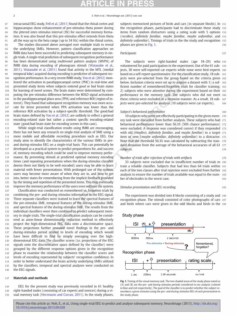
Fig. 1. Timing of the visualmemory task. The two shaded areas of the study phase noted as(A) and (B) are the pre- and during-stimulus periods considered in our analysis (coloredin blue and red respectively). The goal of the classifier is to predict whether the subject re-members a given stimulus using the pre- and during-stimulus EEG of each presentation inthe study phase.

2 E. Noh et al. / NeuroImage xxx (2013) xxx–xxx

UNCO

RREC

intracranial EEG study, Fell et al. (2011) found that the rhinal cortex andhippocampus show enhancement of pre-stimulus theta power duringthe jittered inter-stimulus interval (ISI) for successful memory forma-tion. It was also found that this pre-stimulus effect extends from thetaall the way up to the beta range (up to 34 Hz) within the rhinal cortex.

The studies discussed above averaged over multiple trials to revealthe underlying SMEs. However, pattern classification approaches onfMRI data have been successful in predicting subsequent memory in sin-gle trials. A single-trial prediction of subsequent recognition performancehas been demonstrated using multivoxel pattern analysis (MVPA) offMRI data during encoding of phonogram stimuli (Watanabe et al.,2011). Watanabe et al. (2011) found that activity in the MTL (medialtemporal lobe) acquired during encoding is predictive of subsequent rec-ognition performance. In a very recent fMRI study, Yoo et al. (2012)mon-itored the activation in parahippocampal cortex (PHC) in real-time andpresented study items when subjects entered good or bad brain statesfor learning of novel scenes. The brain states were determined by com-puting the pre-stimulus difference between the BOLD signal activationsin the parahippocampal place area (PPA) and reference ROI (region of in-terest). They found that subsequent recognitionmemorywasmore accu-rate for items presented when PPA activation was lower than thereference ROI activation by a subject-specific threshold. The good/badbrain states defined by Yoo et al. (2012) are unlikely to reflect a generalencoding-related state but rather a context specific encoding-relatedstate (good/bad brain state for encoding scenes in this case).

While single-trial classification results using fMRI are encouraging,there has not been any research on single-trial analysis of SME using amore mobile and affordable recording procedure such as EEG. Ourstudy aims to identify the characteristics of the various SMEs in pre-and during-stimulus EEG on a single-trial basis. This can potentially bedeveloped as a practical system to predict preparedness for, and successof, memory encoding which could be used to improve memory perfor-mance. By presenting stimuli at predicted optimal memory encodingtimes (and repeating presentations when the during-stimulus classifierdeems them not likely to be well encoded) users may be able to learnmaterial with fewer presentations. With prolonged use of the system,users may become more aware of when they are in, and how to getinto, better states for remembering from the implicit feedback providedby the timing and repetition of the presented items. This may eventuallyimprove thememory performance of the users evenwithout the system.

Classification was conducted on remembered vs. forgotten trials bycombining the pre- and during-stimulus information in the EEG signal.Three separate classifiers were trained to learn the spectral features ofthe pre-stimulus SME, temporal features of the during-stimulus SME,and spectral features of the during-stimulus SME. The results from theindividual classifiers were then combined to predict subsequent mem-ory in single trials. The single-trial classification analysis can be consid-ered as anon-linear dimensionality reduction method to effectivelyproject the high-dimensional EEG data onto a discriminative space.These projections further revealed novel findings in the pre- andduring-stimulus period related to levels of encoding which wouldhave been difficult to find by simply averaging over the high-dimensional EEG data. The classifier scores (i.e. projections of the EEGsignals onto the discriminative space defined by the classifier) weregrouped by the different response options given in the recognitionphase to examine the relationship between the classifier scores andlevels of encoding represented by subjects' recognition confidence. Inorder to better understand the brain activity underlying SMEs utilizedby the classifiers, temporal and spectral analyses were conducted onthe EEG signals.

Materials and methods

EEG for the present study was previously recorded in 61 healthyright-handed males (consisting of car experts and novices) during a vi-sual memory task (Herzmann and Curran, 2011). In the study phases,

Please cite this article as: Noh, E., et al., Using single-trial EEG to predict an10.1016/j.neuroimage.2013.09.028

ED P

RO

OF

subjects memorized pictures of birds and cars (in separate blocks). Inthe recognition phases, participants had to discriminate these studyitems from random distractors using a rating scale with 5 options(recollect, definitely familiar, maybe familiar, maybe unfamiliar, anddefinitely unfamiliar). Timings of trials in the the study and recognitionphases are given in Fig. 1.

Participants

The subjects were right-handed males (age 18–29) whovolunteered for paid participation in the experiment. Out of the 61 sub-jects, 30 were self-reported car experts while none were bird expertsbased on a self-report questionnaire. For the classification study, 18 sub-jects were pre-selected from the group based on the criteria givenbelow. Inclusion criteria were set up to acquire a dataset with 1) a suf-ficient number of remembered/forgotten trials for classifier training;2) subjects who were attentive during the experiment based on theirperformance in the memory task. The subjects who did not meetthese criteria were excluded in a stepwise manner. As a result, 18 sub-jects were pre-selected for analysis (10 subjects were car experts).

Subject's behavioral performance10 subjectswhowere not effectively participating in the givenmem-

ory task were discarded from further analysis. These subjects who hadbehavioral performance lower than 56.3% (50% chance performance)were excluded. A response was considered correct if they respondedwith old (recollect, definitely familiar, and maybe familiar) to a targetitem or new (maybe unfamiliar, definitely unfamiliar) to a distractor.Note that the threshold 56.3% was calculated by subtracting the stan-dard deviation from the average of the behavioral accuracies of all 61subjects.

Number of trials after rejection of trials with artifacts33 subjects were excluded due to insufficient number of trials to

train a reliable classifier. Subjects that had less than 64 trials withineach of the two classes after trial rejection were excluded from furtheranalysis to ensure the number of trials available was equal to the num-ber of electrodes in the worst case.

Stimulus presentation and EEG recording

The experiment was divided into 8 blocks consisting of a study andrecognition phase. The stimuli consisted of color photographs of carsand birds where cars were given in the odd blocks and birds in the




TD P

RO

OF

189

190

191

192

193

194

195

196

197

198

199

200

201

202

203

204

205

206

207

208

209

210

211Q4

212

213

214

215

216

217

218

219

220

221

222

223

224

225

226

227

228

229

230

231

232

233

234

235

236

237

238

239

240

241

242

243

244

245

246

247

248

249

250

251

252

253

254

255

256

257

258

259

260

261

262

263

264

265

266

267

268

269

270

271

272

273

274

275

276

277

278

279

280

281

282

283

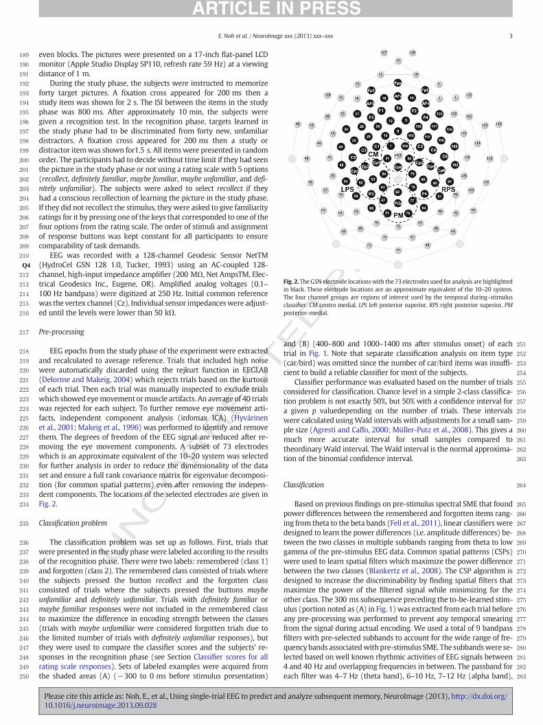
Fig. 2.The GSN electrode locationswith the 73 electrodes used for analysis are highlightedin black. These electrode locations are an approximate equivalent of the 10–20 system.The four channel groups are regions of interest used by the temporal during–stimulusclassifier. CM centro medial, LPS left posterior superior, RPS right posterior superior, PMposterior-medial.

3E. Noh et al. / NeuroImage xxx (2013) xxx–xxx

UNCO

RREC

even blocks. The pictures were presented on a 17-inch flat-panel LCDmonitor (Apple Studio Display SP110, refresh rate 59 Hz) at a viewingdistance of 1 m.

During the study phase, the subjects were instructed to memorizeforty target pictures. A fixation cross appeared for 200 ms then astudy item was shown for 2 s. The ISI between the items in the studyphase was 800 ms. After approximately 10 min, the subjects weregiven a recognition test. In the recognition phase, targets learned inthe study phase had to be discriminated from forty new, unfamiliardistractors. A fixation cross appeared for 200 ms then a study ordistractor itemwas shown for1.5 s. All itemswere presented in randomorder. The participants had to decidewithout time limit if they had seenthe picture in the study phase or not using a rating scale with 5 options(recollect, definitely familiar, maybe familiar, maybe unfamiliar, and defi-nitely unfamiliar). The subjects were asked to select recollect if theyhad a conscious recollection of learning the picture in the study phase.If they did not recollect the stimulus, theywere asked to give familiarityratings for it by pressing one of the keys that corresponded to one of thefour options from the rating scale. The order of stimuli and assignmentof response buttons was kept constant for all participants to ensurecomparability of task demands.

EEG was recorded with a 128-channel Geodesic Sensor NetTM(HydroCel GSN 128 1.0, Tucker, 1993) using an AC-coupled 128-channel, high-input impedance amplifier (200 MΩ, Net AmpsTM, Elec-trical Geodesics Inc., Eugene, OR). Amplified analog voltages (0.1–100 Hz bandpass) were digitized at 250 Hz. Initial common referencewas the vertex channel (Cz). Individual sensor impedanceswere adjust-ed until the levels were lower than 50 kΩ.

Pre-processing

EEG epochs from the study phase of the experiment were extractedand recalculated to average reference. Trials that included high noisewere automatically discarded using the rejkurt function in EEGLAB(Delorme and Makeig, 2004) which rejects trials based on the kurtosisof each trial. Then each trial was manually inspected to exclude trialswhich showed eyemovement ormuscle artifacts. An average of 40 trialswas rejected for each subject. To further remove eye movement arti-facts, independent component analysis (infomax ICA) (Hyvärinenet al., 2001; Makeig et al., 1996) was performed to identify and removethem. The degrees of freedom of the EEG signal are reduced after re-moving the eye movement components. A subset of 73 electrodeswhich is an approximate equivalent of the 10–20 system was selectedfor further analysis in order to reduce the dimensionality of the dataset and ensure a full rank covariance matrix for eigenvalue decomposi-tion (for common spatial patterns) even after removing the indepen-dent components. The locations of the selected electrodes are given inFig. 2.

Classification problem

The classification problem was set up as follows. First, trials thatwere presented in the study phase were labeled according to the resultsof the recognition phase. There were two labels: remembered (class 1)and forgotten (class 2). The remembered class consisted of trials wherethe subjects pressed the button recollect and the forgotten classconsisted of trials where the subjects pressed the buttons maybeunfamiliar and definitely unfamiliar. Trials with definitely familiar ormaybe familiar responses were not included in the remembered classto maximize the difference in encoding strength between the classes(trials with maybe unfamiliar were considered forgotten trials due tothe limited number of trials with definitely unfamiliar responses), butthey were used to compare the classifier scores and the subjects' re-sponses in the recognition phase (see Section Classifier scores for allrating scale responses). Sets of labeled examples were acquired fromthe shaded areas (A) (−300 to 0 ms before stimulus presentation)


Eand (B) (400–800 and 1000–1400 ms after stimulus onset) of eachtrial in Fig. 1. Note that separate classification analysis on item type(car/bird) was omitted since the number of car/bird items was insuffi-cient to build a reliable classifier for most of the subjects.

Classifier performance was evaluated based on the number of trialsconsidered for classification. Chance level in a simple 2-class classifica-tion problem is not exactly 50%, but 50% with a confidence interval fora given p valuedepending on the number of trials. These intervalswere calculated usingWald intervals with adjustments for a small sam-ple size (Agresti and Caffo, 2000; Müller-Putz et al., 2008). This gives amuch more accurate interval for small samples compared totheordinary Wald interval. TheWald interval is the normal approxima-tion of the binomial confidence interval.

Classification

Based on previous findings on pre-stimulus spectral SME that foundpower differences between the remembered and forgotten items rang-ing from theta to the beta bands (Fell et al., 2011), linear classifiers weredesigned to learn the power differences (i.e. amplitude differences) be-tween the two classes in multiple subbands ranging from theta to lowgamma of the pre-stimulus EEG data. Common spatial patterns (CSPs)were used to learn spatial filters which maximize the power differencebetween the two classes (Blankertz et al., 2008). The CSP algorithm isdesigned to increase the discriminability by finding spatial filters thatmaximize the power of the filtered signal while minimizing for theother class. The 300 ms subsequence preceding the to-be-learned stim-ulus (portion noted as (A) in Fig. 1) was extracted from each trial beforeany pre-processing was performed to prevent any temporal smearingfrom the signal during actual encoding. We used a total of 9 bandpassfilters with pre-selected subbands to account for the wide range of fre-quencybands associatedwithpre-stimulus SME. The subbandswere se-lected based on well known rhythmic activities of EEG signals between4 and 40 Hz and overlapping frequencies in between. The passband foreach filter was 4–7 Hz (theta band), 6–10 Hz, 7–12 Hz (alpha band),




T

284

285

286

287

288

289

290

291

292

293

294

295

296

297

298

299

300

301

302

303

304

305

306

307

308

309

310

311

312

313

314

315

316

317

318

319

320

321

322

323

324

325

326

327

328

329

330

331

332

333

334

335

336

337

338

339

340

341

342

343

344

345

346

347

348

349

350

351

352

353

354

355

356

357

358

359

360

361

t1:1

t1:2

t1:3

t1:4

t1:5

t1:6

t1:7

t1:8

t1:9

t1:10

t1:11

t1:12

t1:13

t1:14

t1:15

t1:16

t1:17

t1:18

t1:19

t1:20

t1:21

t1:22

t1:23

t1:24


REC

10–15 Hz, 12–19 Hz (low beta band), 15–25 Hz, 19–30 Hz (high betaband), 25–35 Hz, 30–40 Hz (low gamma band). The overlapping fre-quencies were used to compensate for individual differences in theEEG subbands (Doppelmayr et al., 1998) and timing of the pre-stimulus SME. Subbands with informative patterns for subsequentmemory prediction were identified from the training set and only theclassifiers corresponding to those informative subbands were used toclassify the validation set. The output of the pre-stimulus classifier(denoted as 0 ≤ pA ≤ 1) can be interpreted as the pre-stimulus classifierscore of how good the classifier deems the brain state for rememberingpictures.

Two separate classifiers were designed to extract the temporaland spectral characteristics of the during-stimulus period of theremembered/forgotten trials. Temporal features were learned byexploiting the ERP differences (namely the Dm effect) between thetwo classes in the spatio-temporal domain. The during-stimulus tempo-ral classifierwas trained to learn these features of the EEG data between400 and 800 ms after stimulus presentation from four channel groups(CM centro medial, LPS left posterior superior, RPS right posterior supe-rior, and PM posterior-medial as given in Fig. 2) where the Dm effect isknown to be prominent (Paller andWagner, 2002). Significant spectralSME in the alpha band (7–12 Hz) has been robustly observed in variousmemory experiments (Hanslmayr et al., 2009, 2012; Klimesch et al.,1996b), hence spectral features were extracted (using the CSP algo-rithm) by learning the spatial patterns that best distinguish the alphapower difference between the two classes. The data suggested thatthe early and late alpha SMEs showed considerably different patterns.Hence the during-stimulus spectral classifier learned the power differ-ence between the remembered and forgotten trials by combining theinformation from the two separate time windows (400–800 ms and1000–1400 ms after stimulus presentation). The during-stimulus tem-poral and spectral classifier results were averaged to determine thefinal output of the during-stimulus classifier (denoted as 0 ≤ pB ≤ 1)for a given test trial. This value can be interpreted as the during-stimulus classifier score on the success of the encoding process.

The scores pA and pB from the pre- and during-stimulus classifierswere averaged and compared to the average score of the training setto determine the final label for a given test trial. A given trial was classi-fied as remembered if (pA + pB) / 2 ≥ (mA + mB) / 2 and forgotten if(pA + pB) / 2 b (mA + mB) / 2 where mA and mB are the mean pre-and during-stimulus classifier scores of the training set respectively.The classification accuracies for the pre- and during-classifiers were

UNCO

R

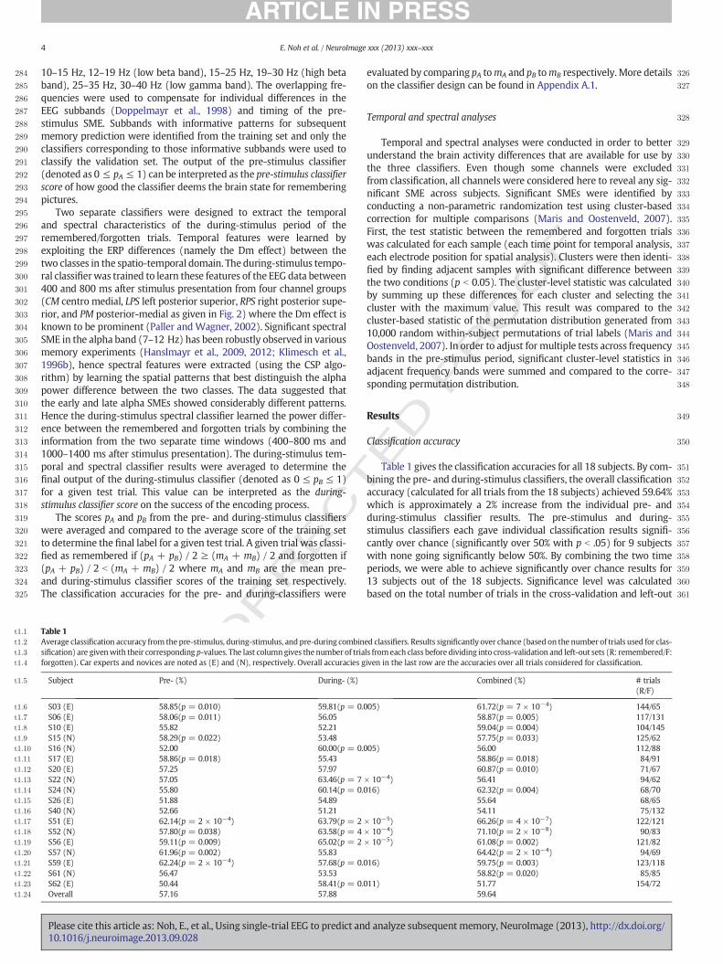
Table 1Average classification accuracy from the pre-stimulus, during-stimulus, and pre-during combinsification) are givenwith their corresponding p-values. The last columngives the number of triaforgotten). Car experts and novices are noted as (E) and (N), respectively. Overall accuracies g

Subject Pre- (%) During- (%)

S03 (E) 58.85(p = 0.010) 59.81(p = 0.0S06 (E) 58.06(p = 0.011) 56.05S10 (E) 55.82 52.21S15 (N) 58.29(p = 0.022) 53.48S16 (N) 52.00 60.00(p = 0.0S17 (E) 58.86(p = 0.018) 55.43S20 (E) 57.25 57.97S22 (N) 57.05 63.46(p = 7S24 (N) 55.80 60.14(p = 0.0S26 (E) 51.88 54.89S40 (N) 52.66 51.21S51 (E) 62.14(p = 2 × 10−4) 63.79(p = 2S52 (N) 57.80(p = 0.038) 63.58(p = 4S56 (E) 59.11(p = 0.009) 65.02(p = 2S57 (N) 61.96(p = 0.002) 55.83S59 (E) 62.24(p = 2 × 10−4) 57.68(p = 0.0S61 (N) 56.47 53.53S62 (E) 50.44 58.41(p = 0.0Overall 57.16 57.88


ED P

RO

OF

evaluated by comparing pA tomA and pB tomB respectively.More detailson the classifier design can be found in Appendix A.1.

Temporal and spectral analyses

Temporal and spectral analyses were conducted in order to betterunderstand the brain activity differences that are available for use bythe three classifiers. Even though some channels were excludedfrom classification, all channels were considered here to reveal any sig-nificant SME across subjects. Significant SMEs were identified byconducting a non-parametric randomization test using cluster-basedcorrection for multiple comparisons (Maris and Oostenveld, 2007).First, the test statistic between the remembered and forgotten trialswas calculated for each sample (each time point for temporal analysis,each electrode position for spatial analysis). Clusters were then identi-fied by finding adjacent samples with significant difference betweenthe two conditions (p b 0.05). The cluster-level statistic was calculatedby summing up these differences for each cluster and selecting thecluster with the maximum value. This result was compared to thecluster-based statistic of the permutation distribution generated from10,000 random within-subject permutations of trial labels (Maris andOostenveld, 2007). In order to adjust for multiple tests across frequencybands in the pre-stimulus period, significant cluster-level statistics inadjacent frequency bands were summed and compared to the corre-sponding permutation distribution.

Results

Classification accuracy

Table 1 gives the classification accuracies for all 18 subjects. By com-bining the pre- and during-stimulus classifiers, the overall classificationaccuracy (calculated for all trials from the 18 subjects) achieved 59.64%which is approximately a 2% increase from the individual pre- andduring-stimulus classifier results. The pre-stimulus and during-stimulus classifiers each gave individual classification results signifi-cantly over chance (significantly over 50% with p b .05) for 9 subjectswith none going significantly below 50%. By combining the two timeperiods, we were able to achieve significantly over chance results for13 subjects out of the 18 subjects. Significance level was calculatedbased on the total number of trials in the cross-validation and left-out

ed classifiers. Results significantly over chance (based on the number of trials used for clas-ls fromeach class before dividing into cross-validation and left-out sets (R: remembered/F:iven in the last row are the accuracies over all trials considered for classification.

Combined (%) # trials(R/F)

05) 61.72(p = 7 × 10−4) 144/6558.87(p = 0.005) 117/13159.04(p = 0.004) 104/14557.75(p = 0.033) 125/62

05) 56.00 112/8858.86(p = 0.018) 84/9160.87(p = 0.010) 71/67

× 10−4) 56.41 94/6216) 62.32(p = 0.004) 68/70

55.64 68/6554.11 75/132

× 10−5) 66.26(p = 4 × 10−7) 122/121× 10−4) 71.10(p = 2 × 10−8) 90/83× 10−5) 61.08(p = 0.002) 121/82

64.42(p = 2 × 10−4) 94/6916) 59.75(p = 0.003) 123/118

58.82(p = 0.020) 85/8511) 51.77 154/72

59.64




362

363

364

365

366

367

368

369

370

371

372

373

374

375

376

377

378

379

380

381

382

383

384

385

386

387

388

389

390

391

392

393


sets for each subject (Agresti and Caffo, 2000; Müller-Putz et al., 2008)as described in Section 2.4.

Out of the 13 subjects with significantly over chance results, 8 sub-jects were self-reported car experts. However, there were no significantdifferences in accuracy for any of the classifiers between the two groupsbased on the Kruskal–Wallis test (pre-: p = 0.33, during-: p = 0.79,combined: p = 0.92), which should not be surprising since memoryfor both birds and cars was included in all analyses.

394

395

396

397

398

399

400

401

402

403

404

405

406

407

408

409

410

411

412

Temporal and spectral SME

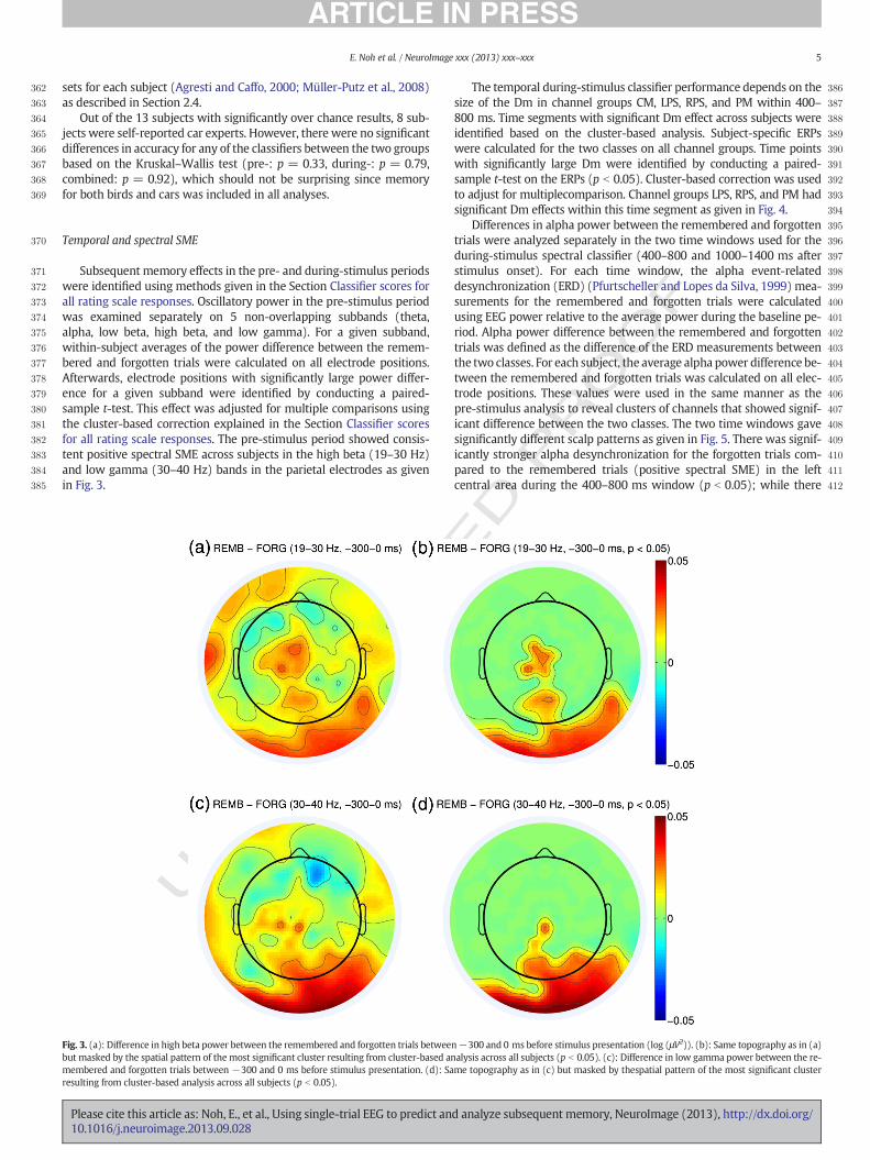
Subsequent memory effects in the pre- and during-stimulus periodswere identified using methods given in the Section Classifier scores forall rating scale responses. Oscillatory power in the pre-stimulus periodwas examined separately on 5 non-overlapping subbands (theta,alpha, low beta, high beta, and low gamma). For a given subband,within-subject averages of the power difference between the remem-bered and forgotten trials were calculated on all electrode positions.Afterwards, electrode positions with significantly large power differ-ence for a given subband were identified by conducting a paired-sample t-test. This effect was adjusted for multiple comparisons usingthe cluster-based correction explained in the Section Classifier scoresfor all rating scale responses. The pre-stimulus period showed consis-tent positive spectral SME across subjects in the high beta (19–30 Hz)and low gamma (30–40 Hz) bands in the parietal electrodes as givenin Fig. 3.

UNCO

RRECT

Fig. 3. (a): Difference in high beta power between the remembered and forgotten trials betweebut masked by the spatial pattern of the most significant cluster resulting from cluster-based anmembered and forgotten trials between −300 and 0 ms before stimulus presentation. (d): Saresulting from cluster-based analysis across all subjects (p b 0.05).


PRO

OF

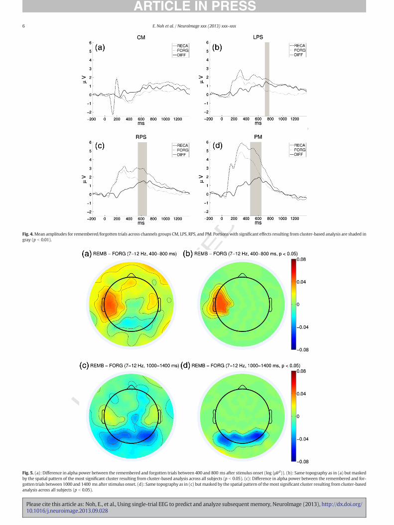
The temporal during-stimulus classifier performance depends on thesize of the Dm in channel groups CM, LPS, RPS, and PM within 400–800 ms. Time segments with significant Dm effect across subjects wereidentified based on the cluster-based analysis. Subject-specific ERPswere calculated for the two classes on all channel groups. Time pointswith significantly large Dm were identified by conducting a paired-sample t-test on the ERPs (p b 0.05). Cluster-based correction was usedto adjust for multiplecomparison. Channel groups LPS, RPS, and PM hadsignificant Dm effects within this time segment as given in Fig. 4.

Differences in alpha power between the remembered and forgottentrials were analyzed separately in the two time windows used for theduring-stimulus spectral classifier (400–800 and 1000–1400 ms afterstimulus onset). For each time window, the alpha event-relateddesynchronization (ERD) (Pfurtscheller and Lopes da Silva, 1999) mea-surements for the remembered and forgotten trials were calculatedusing EEG power relative to the average power during the baseline pe-riod. Alpha power difference between the remembered and forgottentrials was defined as the difference of the ERD measurements betweenthe two classes. For each subject, the average alpha power difference be-tween the remembered and forgotten trials was calculated on all elec-trode positions. These values were used in the same manner as thepre-stimulus analysis to reveal clusters of channels that showed signif-icant difference between the two classes. The two time windows gavesignificantly different scalp patterns as given in Fig. 5. There was signif-icantly stronger alpha desynchronization for the forgotten trials com-pared to the remembered trials (positive spectral SME) in the leftcentral area during the 400–800 ms window (p b 0.05); while there

ED

n−300 and 0 ms before stimulus presentation (log (μV2)). (b): Same topography as in (a)alysis across all subjects (p b 0.05). (c): Difference in low gamma power between the re-me topography as in (c) but masked by thespatial pattern of the most significant cluster




UNCO

RRECTED P

RO

OF

Fig. 4.Mean amplitudes for remembered/forgotten trials across channels groups CM, LPS, RPS, and PM. Portionswith significant effects resulting from cluster-based analysis are shaded ingray (p b 0.01).

Fig. 5. (a): Difference in alpha power between the remembered and forgotten trials between 400 and 800 ms after stimulus onset (log (μV2)). (b): Same topography as in (a) but maskedby the spatial pattern of the most significant cluster resulting from cluster-based analysis across all subjects (p b 0.05). (c): Difference in alpha power between the remembered and for-gotten trials between 1000 and 1400 ms after stimulus onset. (d): Same topography as in (c) butmasked by the spatial pattern of themost significant cluster resulting from cluster-basedanalysis across all subjects (p b 0.05).


Please cite this article as: Noh, E., et al., Using single-trial EEG to predict and analyze subsequent memory, NeuroImage (2013), http://dx.doi.org/10.1016/j.neuroimage.2013.09.028



413

414

415

416

417

418

419

420

421

422

423

424

425

426

427

428

429

430

431

432

433

434

435

436

437

438

439

440

441

442

443

444

445

446

447

448

449

450

451

452

453

454

455

456

457

458

459

460

Table 2 t2:1

t2:2The mean scores given by the pre-stimulus classifiers trained on the 9 separate bandpasst2:3filtered data. Repeated measure ANOVAwas conducted between recollect trials and the 4t2:4other response options. Significant p-values after Bonferroni adjustment for multiplet2:5comparisons are given with * superscripts (⁎: p b 0.012, ⁎⁎: p b 0.005, ⁎⁎⁎: p b 0.001,t2:6⁎⁎⁎⁎: p b 0.0001 Q2).

t2:7Recollect Def fam Maybe fam Maybe unfam Def unfam

t2:84–7 Hz 0.506 0.512 0.506 0.467⁎⁎ 0.459⁎⁎

t2:96–10 Hz 0.506 0.500 0.493 0.466⁎⁎ 0.454⁎⁎⁎

t2:107–12 Hz 0.505 0.498 0.492 0.468⁎⁎ 0.459⁎⁎

t2:1110–15 Hz 0.511 0.488 0.487 0.472⁎ 0.474⁎⁎

t2:1212–19 Hz 0.511 0.498 0.496 0.461⁎⁎⁎ 0.482t2:1315–25 Hz 0.499 0.500 0.478 0.462⁎⁎ 0.471⁎

t2:1419–30 Hz 0.492 0.464 0.463 0.457⁎ 0.481t2:1525–35 Hz 0.511 0.449⁎⁎⁎⁎ 0.460⁎⁎⁎ 0.463⁎⁎⁎⁎ 0.466⁎⁎⁎⁎

t2:1630–40 Hz 0.496 0.456 0.461 0.464 0.478


was significantly stronger alpha desynchronization for the rememberedtrials (negative spectral SME) in the posterior area during the 1000–1400 ms window (p b 0.05).

Classifier scores for all rating scale responses

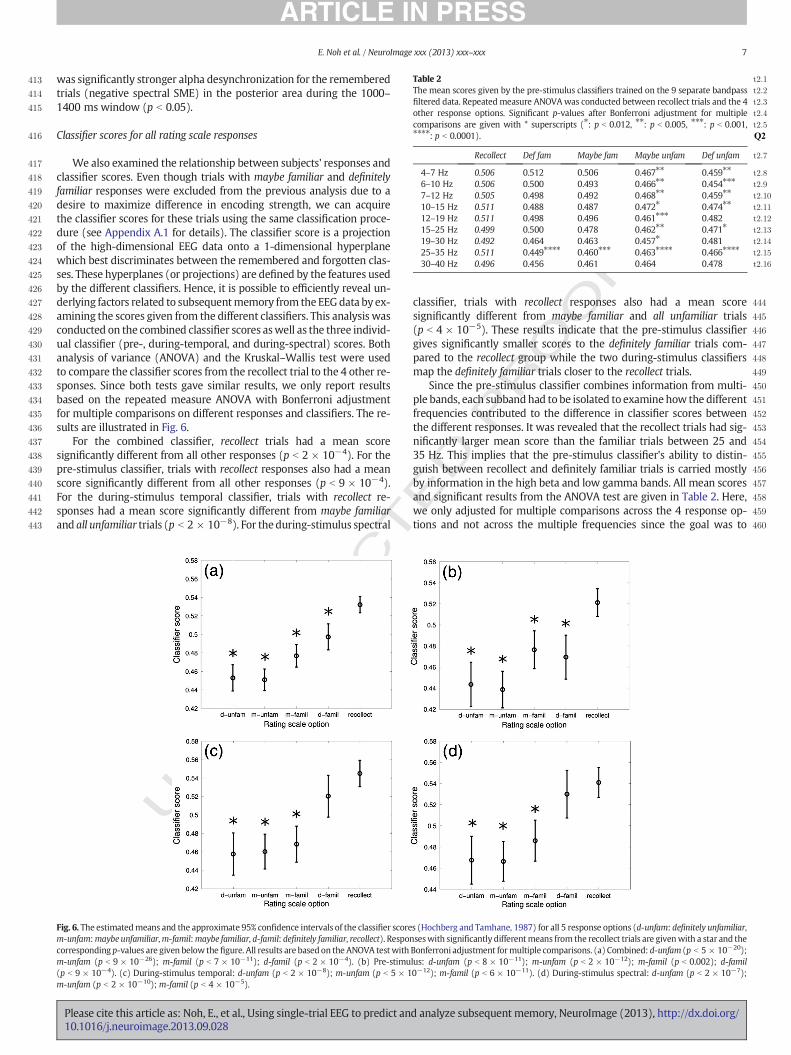
We also examined the relationship between subjects' responses andclassifier scores. Even though trials with maybe familiar and definitelyfamiliar responses were excluded from the previous analysis due to adesire to maximize difference in encoding strength, we can acquirethe classifier scores for these trials using the same classification proce-dure (see Appendix A.1 for details). The classifier score is a projectionof the high-dimensional EEG data onto a 1-dimensional hyperplanewhich best discriminates between the remembered and forgotten clas-ses. These hyperplanes (or projections) are defined by the features usedby the different classifiers. Hence, it is possible to efficiently reveal un-derlying factors related to subsequentmemory from the EEGdata by ex-amining the scores given from the different classifiers. This analysis wasconducted on the combined classifier scores aswell as the three individ-ual classifier (pre-, during-temporal, and during-spectral) scores. Bothanalysis of variance (ANOVA) and the Kruskal–Wallis test were usedto compare the classifier scores from the recollect trial to the 4 other re-sponses. Since both tests gave similar results, we only report resultsbased on the repeated measure ANOVA with Bonferroni adjustmentfor multiple comparisons on different responses and classifiers. The re-sults are illustrated in Fig. 6.

For the combined classifier, recollect trials had a mean scoresignificantly different from all other responses (p b 2 × 10−4). For thepre-stimulus classifier, trials with recollect responses also had a meanscore significantly different from all other responses (p b 9 × 10−4).For the during-stimulus temporal classifier, trials with recollect re-sponses had a mean score significantly different from maybe familiarand all unfamiliar trials (p b 2 × 10−8). For theduring-stimulus spectral

UNCO

RRECT

Fig. 6. The estimatedmeans and the approximate 95% confidence intervals of the classifier scorem-unfam:maybe unfamiliar,m-famil:maybe familiar, d-famil: definitely familiar, recollect). Responcorresponding p-values are given below the figure. All results are based on the ANOVA testwithm-unfam (p b 9 × 10−26); m-famil (p b 7 × 10−11); d-famil (p b 2 × 10−4). (b) Pre-stimu(p b 9 × 10−4). (c) During-stimulus temporal: d-unfam (p b 2 × 10−8); m-unfam (p b 5 × 1m-unfam (p b 2 × 10−10); m-famil (p b 4 × 10−5).


ED P

RO

OF

classifier, trials with recollect responses also had a mean scoresignificantly different from maybe familiar and all unfamiliar trials(p b 4 × 10−5). These results indicate that the pre-stimulus classifiergives significantly smaller scores to the definitely familiar trials com-pared to the recollect group while the two during-stimulus classifiersmap the definitely familiar trials closer to the recollect trials.

Since the pre-stimulus classifier combines information from multi-ple bands, each subbandhad to be isolated to examinehow the differentfrequencies contributed to the difference in classifier scores betweenthe different responses. It was revealed that the recollect trials had sig-nificantly larger mean score than the familiar trials between 25 and35 Hz. This implies that the pre-stimulus classifier's ability to distin-guish between recollect and definitely familiar trials is carried mostlyby information in the high beta and low gamma bands. All mean scoresand significant results from the ANOVA test are given in Table 2. Here,we only adjusted for multiple comparisons across the 4 response op-tions and not across the multiple frequencies since the goal was to

s (Hochberg and Tamhane, 1987) for all 5 response options (d-unfam: definitely unfamiliar,seswith significantly differentmeans from the recollect trials are givenwith a star and theBonferroni adjustment formultiple comparisons. (a) Combined: d-unfam (p b 5 × 10−20);lus: d-unfam (p b 8 × 10−11); m-unfam (p b 2 × 10−12); m-famil (p b 0.002); d-famil0−12); m-famil (p b 6 × 10−11). (d) During-stimulus spectral: d-unfam (p b 2 × 10−7);




461

462

463

464

465

466

467

468

469

470

471

472

473

474

475

476

477

478

479

480

481

482

483

484

485

486

487

488

489

490

491

492

493

494

495

496

497

498

499

500

501

502

503

504

505

506

507

508

509

510

511

512

513

514

Table 3t3:1

t3:2 Themean scores given by the during-stimulus spectral classifiers trained on the individualt3:3 time windows. Repeatedmeasure ANOVAwas conducted between recollect trials and thet3:4 4 other response options. Significant p-values after Bonferroni adjustment for multiplet3:5 comparisons are given with * superscripts (⁎: p b 10−3, ⁎⁎: p b 10−4, ***: p b 10−5).

t3:6 Recollect Def fam Maybe fam Maybe unfam Def unfam

t3:7 400–800 ms 0.543 0.527 0.492⁎ 0.480⁎⁎⁎ 0.475⁎⁎⁎

t3:8 1000–1400 ms 0.524 0.473⁎ 0.449⁎⁎⁎ 0.475⁎⁎ 0.472⁎

Table 4 t4:1

t4:2Themean definitely familiar scores given by the 4 different classifierswere compared to thet4:3maybe familiar and unfamiliar scores using repeated measure ANOVA. Significant p-valuest4:4after Bonferroni adjustment for multiple comparisons are given with * superscriptst4:5(⁎: p b 0.003, ⁎⁎: p b 10−3).

t4:6Classifier Deffam

Maybefam

Maybeunfam

Defunfam

t4:7Group 1 During-temporal (400–800 ms) 0.520 0.468⁎ 0.460⁎⁎ 0.458⁎⁎

t4:8During-alpha (400–800 ms) 0.527 0.492 0.480⁎⁎ 0.475⁎⁎

t4:9Group 2 Pre-[25–35 Hz] (−300–0 ms) 0.449 0.460 0.463 0.466t4:10During-alpha (1000–1400 ms) 0.473 0.449 0.475 0.472


reveal underlying activities that may account for the effect found in thepre-stimulus scores.

The during-stimulus spectral classifier combines information fromtwo distinct timewindows (400–800 and 1000–1400 ms after stimulusonset). Hence, classifier scores were recomputed using classifierstrained on individual windows. The classifier scores for the early win-dow (400–800 ms) showed similar values for the recollect and definitelyfamiliar trials. However, the classifier scores for the later window(1000–1400 ms) were significantly different between the two re-sponses (p = 3 × 10−4). All mean scores and significant results fromthe ANOVA test are given in Table 3.

T515

516

517

518

519

520

521

522

523

524

525

526

527

528

529

530

531

532

533

534

535

536

537

538

539

540

541

542

543

544

545

546

547

548

549

550

551

552

UNCO

RREC

Discussion

These results show that it is possible to successfully predict subse-quent episodicmemory performance based on single-trial scalp EEG ac-tivity recorded before and during item presentation. The prediction rateimproved by 2%, by combining information from the pre- and during-stimulus periods. However, many factors can influence whether a sub-ject will remember a stimulus, not all of which could be controlled inour study including how intrinsically memorable the stimulus is andthe subject's brain state during the recognition phase. These factorsadd noise to the trial labels which may lower classifier accuracy.

There has not been any study that combines information from thepre- and during-stimulus periods of the data to predict subsequentmemory, but the two time periods have been used to predict subse-quent memory separately in two different fMRI studies. Watanabeet al. (2011) showed that it is possible to predict subsequent memorywith approximately 66% accuracy using fMRI data while subjects attendto the stimuli. Since EEG has a lower spatial resolution compared tofMRI a lower prediction rate might be expected (56.8% accuracy forthe during-stimulus classifier). Also, it is difficult to separate the brainsignal prior to and during encoding using fMRI due to the slowness ofthe vascular response. Hence, the classifier may have incorporated in-formation from the pre-stimulus as well as the during-stimulus period.The proportion of subjects with significantly over chance results in ourstudy is comparable to that found by Watanabe et al. (2011) (6 out of13 subjects1 for Watanabe et al. (2011) and 13 out of 18 subjects forthe current study).

Yoo et al. (2012) used the pre-stimulus period of the fMRI data topredict good/bad brain states for learning novel scenes. Their predic-tions gave 48.8% hit rate (percentage of remembered items) duringgood brain states and 41.9% hit rate (percentage of forgotten items) dur-ing bad brain states. Though it is difficult to directly compare the resultsdue to the differences in the experimental paradigm and other settingssuch as recording technique, online/offline2 setting etc., the results fromthe present study are numerically higher than the results from Yoo et al.(2012). The average hit rate during the good brain states (trials with pA

553

554

555

556

557

558

559

1 This was computed by averaging over the main and confirmatory results given inWatanabe et al. (2011) with threshold for chance performance at 66.1% whichwas calcu-lated using methods given in Agresti and Caffo (2000).

2 We refer to a system as onlinewhen it interprets the data and predicts the receptive-ness of a subject to stimuli in real-time. An offline analysis uses data recorded frompast ex-periments where subjects had no knowledge of the system's predictions.


ED P

RO

OF

over 0.5) of the pre-stimulus classifier was 56.5%while the average hitrate during the bad brain states (trials with pA below 0.5) was 42.0%.The hit rate of a random selection of trials was 53.5% across all subjects.

Table 5 shows how often each bandwas chosen for the pre-stimulusclassifier. For example, the first value 0.82 in the table indicates that forsubject S03, frequency band 4–7 Hz gave better than chance trainingerror (and identified as informative) 82% of the time over all cross-validation folds. There are individual differences in the frequencybands utilized by the pre-stimulus classifiers (Table 5). Subjects S26,S40 and S62 have no certain informative band that has better thanchance training error. This suggests that these subjects' EEG data couldbe too noisy for the pre-stimulus classifier to work properly or thepre-stimulus EEG does not contain any useful information (Nijholtet al., 2008). Subjects S16, S20, S24, and S26 have at least one subbandthat is selected 60% of the time, but the pre-stimulus accuracies arenot significantly over chance. This suggests that the training set doesnot well represent the entire data set for these subjects. This may bedue to non-stationarity in the data which may result in non-optimalCSP filters. A consistent cross-subject pre-stimulus spectral SME wasonly observed in the high beta and low gamma bands (Fig. 3).

Our data did not show the significant theta power differenceobserved in Guderian et al. (2009). This may be due to the differencein timing of the pre-stimulus theta SME. Theta difference may occurearlier in the current study due to difference in experiment set-up.Fell et al. (2011) observed that power difference in the theta band oc-curred earlier in time than the higher frequencies. Also, Fellner et al.(2013) demonstrated that pre-stimulus theta SME occurred from −900to −300 ms, but not immediately before stimulus onset. Hence if amajority of the subjects showed theta enhancement in the rememberedtrials prior to −300 ms before stimuli presentation, the data would notshow significant SME in the theta band and only in the higher bands.The pre-stimulus SME observed in the higher frequencies supports thishypothesis. One other possibility is that, due to the small number oftheta cycles possible in the300 mspre-stimuluswindow, thephase shiftsmay be confusable with power differencesmaking the power differencesrelated to subsequent memory difficult to detect.

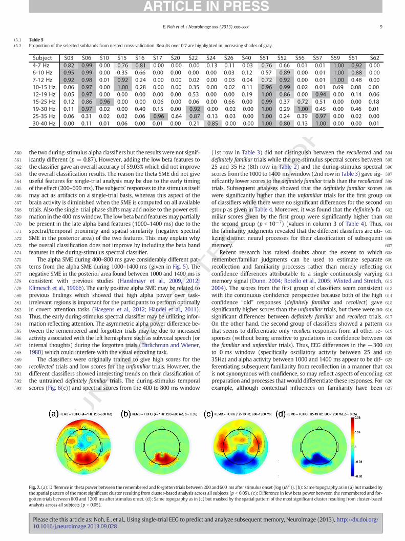
Extra post-hoc spectral analysis in the during-stimulus windowwasconducted on additional frequencies to verify whether spectral SMEfound in previous studies could be identified in the current dataset.Analysis on the theta (4–7 Hz), low beta (12–19 Hz), and high gamma(55–70 Hz) bands revealed that 1) the positive theta SME within theposterior area in the 200–600 ms window and 2) the negative lowbeta SME within the posterior area within the 800–1200 ms windowwere significant (p b 0.05) as given in Fig. 7. These results agree withfindings in Hanslmayr et al. (2009, 2012). Single-trial analysis wasconducted on the theta (4–7 Hz), low beta (12–19 Hz) band featuresto confirm whether information in those bands were classifiable. Theoverall classification results were 49.3% for the theta band and 53.0%for the low beta band. The during-stimulus theta classifier gave signifi-cantly lower results than the two during-stimulus alpha classifiersbased on the rank sum test (p = 0.001) suggesting that the thetaband features were not appropriate for single-trial classification. Theduring-stimulus low beta classifier gave slightly lower accuracy than




T

560

561

562

563

564

565

566

567

568

569

570

571

572

573

574

575

576

577

578

579

580

581

582

583

584

585

586

587

588

589

590

591

592

593

594

595

596

597

598

599

600

601

602

603

604

605

606

607

608

609

610

611

612

613

614

615

616

617

618

619

620

621

622

623

624

625

626

627

Table 5t5:1

t5:2 Proportion of the selected subbands from nested cross-validation. Results over 0.7 are highlighted in increasing shades of gray.


CO

RREC

the two during-stimulus alpha classifiers but the resultswere not signif-icantly different (p = 0.87). However, adding the low beta features tothe classifier gave an overall accuracy of 59.03% which did not improvethe overall classification results. The reason the theta SME did not giveuseful features for single-trial analysis may be due to the early timingof the effect (200–600 ms). The subjects' responses to the stimulus itselfmay act as artifacts on a single-trial basis, whereas this aspect of thebrain activity is diminished when the SME is computed on all availabletrials. Also the single-trial phase shifts may add noise to the power esti-mation in the 400 mswindow. The lowbeta band featuresmay partiallybe present in the late alpha band features (1000–1400 ms) due to thespectral/temporal proximity and spatial similarity (negative spectralSME in the posterior area) of the two features. This may explain whythe overall classification does not improve by including the beta bandfeatures in the during-stimulus spectral classifier.

The alpha SME during 400–800 ms gave considerably different pat-terns from the alpha SME during 1000–1400 ms (given in Fig. 5). Thenegative SME in the posterior area found between 1000 and 1400 ms isconsistent with previous studies (Hanslmayr et al., 2009, 2012;Klimesch et al., 1996b). The early positive alpha SME may be related toprevious findings which showed that high alpha power over task-irrelevant regions is important for the participants to perform optimallyin covert attention tasks (Haegens et al., 2012; Händel et al., 2011).Thus, the early during-stimulus spectral classifier may be utilizing infor-mation reflecting attention. The asymmetric alpha power difference be-tween the remembered and forgotten trials may be due to increasedactivity associated with the left hemisphere such as subvocal speech (orinternal thoughts) during the forgotten trials (Ehrlichman and Wiener,1980) which could interfere with the visual encoding task.

The classifiers were originally trained to give high scores for therecollected trials and low scores for the unfamiliar trials. However, thedifferent classifiers showed interesting trends on their classification ofthe untrained definitely familiar trials. The during-stimulus temporalscores (Fig. 6(c)) and spectral scores from the 400 to 800 ms window

UN

Fig. 7. (a): Difference in theta power between the remembered and forgotten trials between 200the spatial pattern of the most significant cluster resulting from cluster-based analysis across algotten trials between 800 and 1200 ms after stimulus onset. (d): Same topography as in (c) buanalysis across all subjects (p b 0.05).


ED P

RO

OF

(1st row in Table 3) did not distinguish between the recollected anddefinitely familiar trials while the pre-stimulus spectral scores between25 and 35 Hz (8th row in Table 2) and the during-stimulus spectralscores from the 1000 to 1400 mswindow (2nd row in Table 3) gave sig-nificantly lower scores to the definitely familiar trials than the recollectedtrials. Subsequent analyses showed that the definitely familiar scoreswere significantly higher than the unfamiliar trials for the first groupof classifiers while there were no significant differences for the secondgroup as given in Table 4. Moreover, it was found that the definitely fa-miliar scores given by the first group were significantly higher thanthe second group (p b 10−7) (values in column 3 of Table 4). Thus,the familiarity judgments revealed that the different classifiers are uti-lizing distinct neural processes for their classification of subsequentmemory.

Recent research has raised doubts about the extent to whichremember/familiar judgments can be used to estimate separaterecollection and familiarity processes rather than merely reflectingconfidence differences attributable to a single continuously varyingmemory signal (Dunn, 2004; Rotello et al., 2005; Wixted and Stretch,2004). The scores from the first group of classifiers seem consistentwith the continuous confidence perspective because both of the highconfidence “old” responses (definitely familiar and recollect) gavesignificantly higher scores than the unfamiliar trials, but there were nosignificant differences between definitely familiar and recollect trials.On the other hand, the second group of classifiers showed a patternthat seems to differentiate only recollect responses from all other re-sponses (without being sensitive to gradations in confidence betweenthe familiar and unfamiliar trials). Thus, EEG differences in the −300to 0 ms window (specifically oscillatory activity between 25 and35Hz) and alpha activity between 1000 and 1400 ms appear to be dif-ferentiating subsequent familiarity from recollection in a manner thatis not synonymous with confidence, so may reflect aspects of encodingpreparation and processes that would differentiate these responses. Forexample, although contextual influences on familiarity have been

and600 ms after stimulus onset (log (μV2)). (b): Same topography as in (a) butmaskedbyl subjects (p b 0.05). (c): Difference in low beta power between the remembered and for-t masked by the spatial pattern of themost significant cluster resulting from cluster-based




T

628

629

630

631

632

633

634

635

636

637

638

639

640

641

642

643

644

645

646

647

648

649

650

651

652

653

654

655

656

657

658

659

660

661

662

663

664

665

666

667

668

669

670

671

672

673

674

675

676

677

678

679

680

681

682

683

684

685

686

687

688

689

690

691

692

693

694

695

696

697

698

699

700

701

702

703

704

705

706

707

708

709

710

711

712

713

714

715

716

717

718719720721722

723

724

725

726

727

728

729

730

731

732

733

734

735

736

737

738

739

740

741

742

743

744

3 The soft margin SVM classifier for a two-class classification problem gives a pair ofscores (p1 and p2) corresponding to the probability of potential class membership wherep1 + p2 = 1. Here, we consider the output of the classifier to be p = p1 which representsthe probability an example is a remembered trial (classified as remembered if p ≥ 0.5 andforgotten if p b 0.5).


UNCO

RREC

demonstrated (Addante et al., 2012; Elfman et al., 2008; Mollison andCurran, 2012; Speer and Curran, 2007), contextual influences are wide-ly regarded to be stronger on recollection than familiarity (Davachiet al., 2001; Cansino et al., 2002; Ranganath et al., 2004; Duarte et al.,2004; Summerfield and Mangels, 2005). Perhaps pre-stimulus activitybetween 25 and 35 Hz is important for encoding contextual informa-tion, which may include contextual information taken from the pre-stimulus period itself (e.g., whatever the subject was thinking aboutprior to encoding). Also, during stimulus presentation, the brain activitymay shift from encoding the stimulus early in the trial to also encodingthe contextual information in that period.

We cannot completely rule out the possibility that the pre-stimulusclassifiermay be using the brain activity of the evoked response to thefix-ation cross rather than the ongoing pre-stimulus neural activities for clas-sification. However the pre-stimulus ERP did not show any significantdifference between the remembered and forgotten trials. This decreasesthe possibility that the evoked response from the fixation cross holdsany information that discriminates between the two classes. In a follow-up study, the effects of these different signals on classification resultswill be further investigated using an appropriate experiment paradigm.

In summary, this study shows that pre- and during-stimulus EEGcan be used to predict subsequent memory performance. We discov-ered that the pre-stimulus classifier (especially in frequencies around25–35 Hz) using the −300–0 ms window and during-stimulus alphaband classifier using the 1000–1400 mswindowdistinguished recollec-tion from familiarity, whereas the during-stimulus temporal and alphaband classifiers using the 400–800 ms did not. These results suggestthat 1) the brain activity before item presentation contributes to howwell context gets encoded with the upcoming item and 2) the brain ac-tivity during item presentation initially focuses on item encoding thenshifts to also encoding the contextual information. Finally, these find-ings could provide an inexpensive and non-invasive way to monitorlearning preparedness to optimally determine the time to present astimulus and present the stimulus again at a later time point if theencoding process is unsuccessful.

Acknowledgments

This research was funded by NSF grants # CBET-0756828 and # IIS-1219200, NIH grant MH64812, NSF grants # SBE-0542013 and # SMA-1041755 to the Temporal Dynamics of Learning Center (an NSF Scienceof Learning Center), and a James S. McDonnell Foundation grant to thePerceptual Expertise Network, and the KIBM (Kavli Institute of Brainand Mind) Innovative Research Grant. We would like to thank MartaKutas and Tom Urbach for helpful comments on the manuscript.

Appendix A

Appendix A.1. Classifier training procedure

Depending on the performance (recollection rate) of each subject,the difference between the number of trials for the remembered classand the forgotten class ranged from 1 to 82. Rather than discarding sub-jects with unbalanced classes (Watanabe et al., 2011), enough trialsfrom the larger class were set aside from training as the left-out set tobalance the number of trials per class in the cross-validation set. Trialsin the left-out set were evenly distributed over time (epochs andblocks) to minimize the effect of drift or bias in the cross-validationset. The cross-validation set was evaluated based on a balanced leave-two-out cross-validation procedure where one example from eachclass is randomly selected and left out of any training procedure as thevalidation set (to ensure they were not used in any manner to trainthe classifier) while the remaining trials are used as the training setfor each fold. The left-out set was evaluated using the classifier trainedfrom all trials in the cross-validation set. This procedure allowed us toeliminate any effect from unbalanced classes during classifier training


ED P

RO

OF

while conducting classification on all available trials. The classifiers tocompute the classifier scores for trials with definitely familiar andmaybe familiar responseswere also trained for each subject using all tri-als in the cross-validation set.

Appendix A.1.1. Pre-stimulus classifierZero-phase filtering was used to extract desired subband signals

while preserving the timing of the features from the pre-stimulus peri-od. Since a non-causal filter was used, the 300 ms subsequence preced-ing the to-be-learned stimuluswas extracted before filtering to preventany temporal smearing from the signal during actual encoding. 25 extrasamples in the 100 ms period before the fixation crosswere included toestimate a better covariance matrix for CSP analysis. 20 tap zero-phaseFIR filters were used to design the 9 bandpass filters (4–7 Hz, 6–10 Hz,7–12 Hz, 10–15 Hz, 12–19 Hz, 15–25 Hz, 19–30 Hz, 25–35 Hz, and30–40 Hz). Nine separate passband signals were generated for eachtrial through this procedure.

Separate classifiers were constructed using the training sets of the 9subbands. For each subband group, CSP filters were learned to extractfeatures that maximally discriminate between the remembered (class1) and forgotten (class 2) trials. CSP is a supervised dimensionality re-duction algorithm commonly used for EEG classification. CSP utilizesthe covariance matrices of the two classes (estimated from thebandpass filtered EEG data) to find spatial filters that maximize the var-iance of spatially filtered signals under one condition while minimizingit for the other condition. The 73 channels of EEG data were used to es-timate the spatial filters. Three spatial filters were selected from eachclass resulting in 6 filtered signals as in Blankertz et al. (2008). The logpower was calculated by

Pi ¼1Tlog

XT

t¼1

s2i;t ðA:1Þ

where si,t is the sample for time t from filtered signal i (i = 1,…, 6 andt = 1,…, T where T is the number of samples within an example). Thisresulted in a 6 dimensional vector P ¼ P1; :::; P6½ � for each trial.

The soft margin3 support vector classifier machine (v-SVM) (Changand Lin, 2001)with a linear kernel was used to classify the 6 dimension-al vectors. LIBSVM (Chang and Lin, 2011)was utilized for this part of thesimulation. The parameter 0 ≤ v ≤ 1 can be interpreted as an upperbound on the proportion of margin errors and the lower bound onproportion of support vectors. v was selected based on a 4-fold cross-validation on the set P

� �acquired from the training set.

The training error for each subband group was calculated byconducting a balanced cross-validation on the training set. Subbandgroups that gave better than chance (with p b 0.10) training error wereidentified as informative. If none of the subbands gave better than chancetraining error, all 9 subbands were selected. The decision of the pre-stimulus classifier for a given trial in the validation or left-out set (pA)was determined by averaging over the scores given by SVM classifiersfrom all informative subbands. This meta-classification approach wasused based on previous studies which found that meta-classificationstrategies generally outperform single classifiers (Dornhege et al., 2004;Hammon and de Sa, 2007).

Appendix A.2. During-stimulus classifierDifferent bandpass filters and spatial filters were used to extract fea-

tures for the during-stimulus temporal and spectral classifiers.In order to learn the ERP patterns of the Dmeffect, the baselined sig-

nal (baseline offset corrected using −200 to 0 ms of each trial) was




745

746

747

748

749

750

751

752

753

754

755

756

757

758

759

760

761

762

763

764

765

766

767

768

769

770

771

772

773

774

775776777778779780781782783784785786787788789790791792793794795796797798799800801802803804805806807808809

810811812813814815816817818819820821822823824825826827828829830831832833834Q6835836837838839840841842843844845846847


bandpass filtered between 0.1 and 5 Hz using a 40 tap zero-phase FIRfilter. Based on previous research on the Dm, the 400–800 ms timewin-dow and four channel groups were selected for evaluation (CM centromedial, LPS left posterior superior, RPS right posterior superior, and PMposterior-medial as given in Fig. 2). Mean amplitudes for each channelgroup were calculated by averaging over the channels within eachgroup. For each channel group, a 5-dimensional template forremembered/forgotten trials was calculated. First, the ERP of the train-ing set was calculated for each class. The dimensionality of the ERPwas reduced to 5 by averaging over 80 ms length non-overlappingwin-dows between 400 and 800 ms. Finally, templates from all channelgroups were concatenated to create a 20-dimensional template forremembered/forgotten trials. A soft margin4 linear classifier using LDA(linear discriminant analysis) was trained based on these templates andthe dispersion of the training examples. LDA is a simple classifier whichis commonly used to classify ERP components (Blankertz et al., 2011).

In order to isolate the alpha band of the EEG signal, the baselined sig-nal (baseline offset corrected using −200 to 0 ms of each trial) wasbandpass filtered between 7 and 12 Hzwith a 40 tap zero-phase FIR fil-ter. The data were divided into two timewindows (400–800 and 1000–1400 ms after the cue). For each time window, 6 CSP filters (3 for eachclass)were learned using the 73 channel EEG data and the log powers ofthe spatially filtered signals were computed. The log power values werecombined to acquire a 12 dimensional feature vector for each trial. Thesoft margin v-SVM with a linear kernel was used for classification. TheCSP procedure, log power calculation, and v parameter selection follow-ed the procedures given in Appendix A.1.1.

The decision of the during-stimulus classifier (pB) was determined byaveraging over the scores given by the temporal and spectral classifiers.

T

848849850851852853854855856857858859860861862863Q5864865866867868869870871872873874875876877878879880881882883884885886887

UNCO

RREC

References

Addante, R.J., Ranganath, C., Yonelinas, A., 2012. Examining ERP correlates of recognitionmemory: evidence of accurate source recognition without recollection. NeuroImage62, 439–450.

Agresti, A., Caffo, B., 2000. Simple and effective confidence intervals for proportions anddifferences of proportions result from adding two successes and two failures. Am.Stat. 54, 280–288.

Blankertz, B., Tomioka, R., Lemm, S., Kawanabe, M., Muller, K.R., 2008. Optimizing spatialfilters for robust EEG single-trial analysis. IEEE Signal Process. Mag. 25, 41–56.

Blankertz, B., Lemm, S., Treder, M.S., Haufe, S., Müller, K.R., 2011. Single-trial analysis andclassification of ERP components — a tutorial. NeuroImage 56, 814–825.

Cansino, S., Maquet, P., Dolan, R.J., Rugg, M.D., 2002. Brain activity underlying encodingand retrieval of source memory. Cereb. Cortex 12, 1048–1056.

Chang, C.C., Lin, C.J., 2001. Training v-support vector classifiers: theory and algorithms.Neural Comput. 13, 2119–2147.

Chang, C.C., Lin, C.J., 2011. LIBSVM: a library for support vector machines. ACM Trans.Intell. Syst. Technol. 2 (27), 1–27 (27).

Davachi, L., Maril, A., Wagner, A.D., 2001. When keeping in mind supports later bringingto mind: neural markers of phonological rehearsal predict subsequent remembering.J. Cogn. Neurosci. 13, 1059–1070.

Delorme, A., Makeig, S., 2004. EEGLAB: an open source toolbox for analysis of single-trialEEG dynamics. J. Neurosci. Methods 134, 9–21.

Doppelmayr, M., Klimesch, W., Pachinger, T., Ripper, B., 1998. Individual differences inbrain dynamics: important implications for the calculation of event-related bandpower. Biol. Cybern. 79, 49–57.

Dornhege, G., Blankertz, B., Curio, G., Müller, K.R., 2004. Boosting bit rates in noninvasiveEEG single-trial classifications by feature combination and multiclass paradigms. IEEETrans. Biomed. Eng. 51, 993–1002.

Duarte, A., Ranganath, C., Winward, L., Hayward, D., Knight, R.T., 2004. Dissociable neuralcorrelates for familiarity and recollection during the encoding and retrieval of pic-tures. Cogn. Brain Res. 18, 255–272.

Dümbgen, L., Igl, B.W., Munk, A., 2008. P-values for classification. Electron. J. Stat. 2,468–493.

Dunn, J.C., 2004. Remember-know: a matter of confidence. Psychol. Rev. 111, 524–542.Ehrlichman, H., Wiener, M.S., 1980. EEG asymmetry during covert mental activity. Psy-

chophysiology 17, 228–235.
888889890891892893894895
4 The probability output for the softmargin LDA classifierwas calibrated based on a per-mutation test with plug-in estimator of Bayesian likelihood ratios for the standard homo-scedastic Gaussianmodel (Dümbgen et al., 2008). As in the soft margin SVM classifier, theclassifier gives a pair of numbers (p1 and p2) corresponding to the probability of classmembership. We consider the output of the classifier to be p = p1 which represents theprobability an example is a remembered trial.


ED P

RO

OF

Elfman, K.W., Parks, C.M., Yonelinas, A.P., 2008. Testing a neurocomputational model ofrecollection, familiarity, and source recognition. J. Exp. Psychol. Learn. Mem. Cogn.34, 752–768.

Fell, J., Ludowig, E., Staresina, B.P., Wagner, T., Kranz, T., Elger, C.E., Axmacher, N., 2011.Medial temporal theta/alpha power enhancement precedes successful memoryencoding: evidence based on intracranial EEG. J. Neurosci. 31, 5392–5397.

Fellner, M.C., Bäuml, K.H.T., Hanslmayr, S., 2013. Brain oscillatory subsequent memory ef-fects differ in power and long-range synchronization between semantic and survivalprocessing. NeuroImage 79, 361–370.

Gruber, M.J., Otten, L.J., 2010. Voluntary control over prestimulus activity related toencoding. J. Neurosci. 30, 9793–9800. http://dx.doi.org/10.1523/JNEUROSCI.0915-10.2010.

Gruber, M.J., Watrous, A.J., Ekstrom, A.D., Ranganath, C., Otten, L.J., 2013. Expected rewardmodulates encoding-related theta activity before an event. NeuroImage 68–74.

Guderian, S., Schott, B.H., Richardson-Klavehn, A., Duezel, E., 2009. Medial temporal thetastate before an event predicts episodic encoding success in humans. Proc. Natl. Acad.Sci. 106, 5365–5370.

Haegens, S., Luther, L., Jensen, O., 2012. Somatosensory anticipatory alpha activity in-creases to suppress distracting input. J. Cogn. Neurosci. 24, 677–685.

Hammon, P.S., de Sa, V.R., 2007. Pre-processing and meta-classification for brain-computer interfaces. IEEE Trans. Biomed. Eng. 54, 518–525.

Händel, B.F., Haarmeier, T., Jensen, O., 2011. Alpha oscillations correlate with the success-ful inhibition of unattended stimuli. J. Cogn. Neurosci. 23, 2494–2502.

Hanslmayr, S., Staudigl, T., 2013. How brain oscillations form memories — a processingbased perspective on oscillatory subsequent memory effects. NeuroImage.

Hanslmayr, S., Spitzer, B., Bäuml, K.H., 2009. Brain oscillations dissociate betweensemantic and nonsemantic encoding of episodic memories. Cereb. Cortex 19,1631–1640.

Hanslmayr, S., Staudigl, T., Fellner, M.C., 2012. Oscillatory power decreases and long-termmemory: The information via desynchronization hypothesis. Front. Hum. Neurosci. 6.

Herzmann, G., Curran, T., 2011. Experts' memory: an ERP study of perceptual expertise ef-fects on encoding and recognition. Mem. Cogn. 39, 412–432.

Hochberg, Y., Tamhane, A.C., 1987. Multiple Comparison Procedures. John Wiley & Sons,Inc., New York, NY, USA.

Hyvärinen, A., Karhunen, J., Oja, E., 2001. Independent ComponentAnalysis.Wiley, NewYork.Johnson, R.J., 1995. Event-related potential insights into the neurobiology of memory sys-

tems. In: Boller, F., Grafman, J. (Eds.), The Handbook of Neuropsychology, 10. ElsevierScience Publishers, Amsterdam, pp. 134–164.

Klimesch, W., Doppelmayr, M., Russegger, H., Pachinger, T., 1996a. Theta band power inthe human scalp eeg and the encoding of new information. Neuroreport 17,1235–1240.

Klimesch, W., Schimke, H., Doppelmayr, M., Ripper, B., Schwaiger, J., Pfurtscheller, G.,1996b. Event-related desynchronization (ERD) and the Dm effect: does alphadesynchronization during encoding predict later recall performance? Int.J. Psychophysiol. 24, 47–60.

Makeig, S., Bell, A.J., Jung, T.P., Sejnowski, T.J., 1996. Independent component analysis ofelectroencephalographic data. Adv. Neural Inf. Process. Syst. 8, 145–151.

Maris, E., Oostenveld, R., 2007. Nonparametric statistical testing of EEG- and MEG-data.J. Neurosci. Methods 164, 177–190.

Mollison, M.V., Curran, T., 2012. Familiarity in source memory. Neuropsychologia 50,2546–2565.

Müller-Putz, G., Scherer, R., Brunner, C., Leeb, R., Pfurtscheller, G., 2008. Better than ran-dom? A closer look on BCI results. Int. J. Bioelectromagn. 10, 52–55.

Nijholt, A., Tan, D., Pfurtscheller, G., Brunner, C., del R. Millán, J., Allison, B., Graimann,B., Popescu, F., Blankertz, B., Müller, K.R., 2008. Brain-computer interfacing forintelligent systems. IEEE Intell. Syst. 23, 72–79. http://dx.doi.org/10.1109/MIS.2008.41.

Otten, L.J., Quayle, A.H., Akram, S., Ditewig, T.A., Rugg, M.D., 2006. Brain activity before anevent predicts later recollection. Nat. Neurosci. 9, 489–491.

Otten, L.J., Quayle, A.H., Puvaneswaran, B., 2010. Prestimulus subsequent memory effectsfor auditory and visual events. J. Cogn. Neurosci. 22, 1212–1223.

Paller, K.A., Wagner, A.D., 2002. Observing the transformation of experience into memory.Trends Cogn. Sci. 6, 93–102.

Paller, K.A., Kutas, M., Mayes, A.R., 1987. Neural correlates of encoding in an incidentallearning paradigm. Electroencephalogr. Clin. Neurophysiol. 67, 360–371. http://dx.doi.org/10.1016/0013-4694(87)90124-6.

Park, H., Rugg, M.D., 2010. Neural correlates of encodingwithin- and across-domain inter-item associations. J. Cogn. Neurosci. 9, 2533–2543.

Pfurtscheller, G., Lopes da Silva, F.H., 1999. Event-related EEG/MEG synchronization anddesynchronization: basic principles. Clin. Neurophysiol. 110, 1842–1857.

Ranganath, C., Yonelinas, A.P., Cohen, M.X., Dy, C.J., Tom, S.M., D'Esposito, M., 2004. Disso-ciable correlates of recollection and familiarity within the medial temporal lobes.Neuropsychologia 42, 2–13.

Rotello, C.M., Macmillan, N.A., Reeder, J.A., Wong, M., 2005. The remember response: sub-ject to bias, graded, and not a process-pure indicator of recollection. Psychon. Bull.Rev. 12, 865–873.

Sanquist, T.F., Rohrbaugh, J.W., Syndulko, K., Lindsley, D.B., 1980. Electrocortical signs oflevels of processing: perceptual analysis and recognition memory. Psychophysiology17, 568–576.

Sederberg, P.B., Kahana, M.J., Howard, M.W., Donner, E.J., Madsen, J.R., 2003. Theta andgamma oscillations during encoding predict subsequent recall. J. Neurosci. 23,10809–10814.

Speer, N.K., Curran, T., 2007. ERP correlates of familiarity and recollection processes invisual associative recognition. Brain Res. 1174, 97–109.

Staudigl, T., Hanslmayr, S., 2013. Theta oscillations at encoding mediate the context-dependent nature of human episodic memory. Curr. Biol. 23, 1101–1106.


http://dx.doi.org/10.1523/JNEUROSCI.0915-10.2010

http://dx.doi.org/10.1523/JNEUROSCI.0915-10.2010

http://dx.doi.org/10.1109/MIS.2008.41

http://dx.doi.org/10.1109/MIS.2008.41

http://dx.doi.org/10.1016/0013-4694(87)90124-6



896897898899900901

902903904905906907

909


Summerfield, C., Mangels, J.A., 2005. Coherent theta-band EEG activity predicts item-context binding during encoding. NeuroImage 24, 692–703.

Watanabe, T., Hirose, S., Wada, H., Katsura, M., Chikazoe, J., Jimura, K., Imai, Y., Machida, T.,Shirouzu, I., Miyashita, Y., Konishi, S., 2011. Prediction of subsequent recognition per-formance using brain activity in the medial temporal lobe. NeuroImage 54,3085–3092.

UNCO

RRECT

908


Wixted, J.T., Stretch, V., 2004. In defense of the signal-detection interpretation ofremember/know judgments. Psychon. Bull. Rev. 11, 616–641.

Yoo, J.J., Hinds, O., Ofen, N., Thompson, T.W., Whitfield-Gabrieli, S., Triantafyllou, C.,Gabrieli, J.D., 2012. When the brain is prepared to learn: Enhancing human learningusing real-time fMRI. NeuroImage 59, 846–852. http://dx.doi.org/10.1016/j.neuroimage.2011.07.063.

ED P

RO

OF






using single-trial eeg to predict and analyze subsequent memory

Documents