using semantics in xml query processing · zhifeng bao, jiaheng lu, tok wang ling, liang xu, huayu...

$: USING SEMANTICS IN XML QUERY PROCESSING · Zhifeng Bao, Jiaheng Lu, Tok Wang Ling, Liang Xu, Huayu Wu. \An E ec-tive Object-Level XML Keyword Search". The 15th International Conference$
USING SEMANTICS IN XML QUERY PROCESSING

WU HUAYU

Bachelor of Computing (Honors)

National University of Singapore

A THESIS SUBMITTED

FOR THE DEGREE OF DOCTOR OF PHILOSOPHY

DEPARTMENT OF COMPUTER SCIENCE

NATIONAL UNIVERSITY OF SINGAPORE

2011

i

ACKNOWLEDGEMENT

This thesis would not have been possible without the guidance and the help of many

people who provided their valuable assistance to the preparation and completion

of my study.

First and foremost, my sincerest gratitude goes to my supervisor Professor Ling

Tok Wang. Professor Ling first introduced me to the area of database research.

He taught me how to identify research problems, how to formalize problems, and

how to write research papers. His supervision and advice exceptionally inspires my

growth from a student in class, to a qualified Ph.D. candidate for scientific research.

I gratefully acknowledge Professor Gillian Dobbie who gave me insightful advice

on my research work. I benefited a lot from her patient guidance on paper writing.

I would like to thank Professor Chan Chee Yong and Professor Wynne Hsu for

serving as my thesis advisory committee members and providing valuable advice

on my work. I would like to thank Bao Zhifeng and Xu Liang who worked with

me in a group to discuss problems and work on interesting research topics. Many

thanks go to my friends in School of Computing. The years we spent together will

become a beautiful memory in my mind, forever.

ii

Last but not least, I wish to express my appreciation to my family, especially

my wife Lisa, for their continuous love, support and understanding. They gave me

the courage and strength to overcome any difficulties in my life.

CONTENTS

Acknowledgement i

Abstract vii

List of publications x

1 Introduction 1

1.1 Data Model . . . . . . . . . . . . . . . . . . . . . . . . . . . . . . . 2

1.2 XML query . . . . . . . . . . . . . . . . . . . . . . . . . . . . . . . 3

1.2.1 From XPath and XQuery query to twig pattern query . . . . 4

1.2.2 Twig pattern matching . . . . . . . . . . . . . . . . . . . . . 6

1.3 Document labeling and inverted list . . . . . . . . . . . . . . . . . . 8

1.4 Our research scope and contributions . . . . . . . . . . . . . . . . . 12

1.5 Thesis organization . . . . . . . . . . . . . . . . . . . . . . . . . . . 14

2 Literature Review 16

2.1 Query processing over XML tree . . . . . . . . . . . . . . . . . . . . 16

iii

iv

2.1.1 The relational approach . . . . . . . . . . . . . . . . . . . . 17

2.1.2 The native approach . . . . . . . . . . . . . . . . . . . . . . 22

2.1.3 Comparison between the relational approach and the native

approach . . . . . . . . . . . . . . . . . . . . . . . . . . . . . 28

2.1.4 Hybrid management of relational data and XML data . . . . 29

2.2 Query processing over XML graph . . . . . . . . . . . . . . . . . . . 30

2.3 Summary of related work . . . . . . . . . . . . . . . . . . . . . . . . 32

3 A semantic approach for twig pattern query processing 35

3.1 Introduction and motivation . . . . . . . . . . . . . . . . . . . . . . 36

3.2 VERT algorithm . . . . . . . . . . . . . . . . . . . . . . . . . . . . 40

3.2.1 Object-related semantics in XML data . . . . . . . . . . . . 40

3.2.2 An overview of VERT . . . . . . . . . . . . . . . . . . . . . 43

3.2.3 Document parsing in VERT . . . . . . . . . . . . . . . . . . 44

3.2.4 Query processing in VERT . . . . . . . . . . . . . . . . . . . 48

3.2.5 Analysis of VERT . . . . . . . . . . . . . . . . . . . . . . . . 51

3.3 Semantic optimizations . . . . . . . . . . . . . . . . . . . . . . . . . 54

3.3.1 Optimization 1: object/property table . . . . . . . . . . . . 54

3.3.2 Optimization 2: object table . . . . . . . . . . . . . . . . . . 56

3.3.3 Optimization 3: relationship table . . . . . . . . . . . . . . . 59

3.4 Query across multiple twig patterns . . . . . . . . . . . . . . . . . . 63

3.4.1 Query plan selection . . . . . . . . . . . . . . . . . . . . . . 65

3.5 Experiments . . . . . . . . . . . . . . . . . . . . . . . . . . . . . . . 67

3.5.1 Settings . . . . . . . . . . . . . . . . . . . . . . . . . . . . . 67

3.5.2 Comparison with Schema-based Relational Approach . . . . 68

3.5.3 Comparison with TwigStack . . . . . . . . . . . . . . . . . . 70

3.6 Summary . . . . . . . . . . . . . . . . . . . . . . . . . . . . . . . . 74

v

4 Enhancing twig pattern semantics for complex output information 75

4.1 Introduction . . . . . . . . . . . . . . . . . . . . . . . . . . . . . . . 76

4.2 Query node characteristics . . . . . . . . . . . . . . . . . . . . . . . 79

4.2.1 Purpose of query nodes . . . . . . . . . . . . . . . . . . . . . 80

4.2.2 Optionality of query nodes . . . . . . . . . . . . . . . . . . . 80

4.2.3 Occurrence of output information . . . . . . . . . . . . . . . 81

4.3 TP+Output: an extension of twig pattern . . . . . . . . . . . . . . 82

4.3.1 Predicate node . . . . . . . . . . . . . . . . . . . . . . . . . 83

4.3.2 Optional-predicate node . . . . . . . . . . . . . . . . . . . . 84

4.3.3 Output node . . . . . . . . . . . . . . . . . . . . . . . . . . 84

4.3.4 Optional-output node . . . . . . . . . . . . . . . . . . . . . . 85

4.3.5 Predicated-output node . . . . . . . . . . . . . . . . . . . . 85

4.3.6 Optional-predicated-output node . . . . . . . . . . . . . . . 86

4.3.7 Discussion . . . . . . . . . . . . . . . . . . . . . . . . . . . . 87

4.4 VERTO to process TP+Output queries . . . . . . . . . . . . . . . . 88

4.4.1 Analysis . . . . . . . . . . . . . . . . . . . . . . . . . . . . . 93

4.5 Experiments . . . . . . . . . . . . . . . . . . . . . . . . . . . . . . . 94

4.5.1 Experimental settings . . . . . . . . . . . . . . . . . . . . . . 94

4.5.2 Compare TP+Output with TP and GTP . . . . . . . . . . . 95

4.5.3 Scalability of VERTO . . . . . . . . . . . . . . . . . . . . . . 97

4.5.4 Comparison with XQuery processors . . . . . . . . . . . . . 97

4.6 Summary . . . . . . . . . . . . . . . . . . . . . . . . . . . . . . . . 99

5 Performing grouping and aggregation in XML queries 101

5.1 Introduction . . . . . . . . . . . . . . . . . . . . . . . . . . . . . . . 102

5.2 Related work on XML grouping . . . . . . . . . . . . . . . . . . . . 105

5.3 Query expression . . . . . . . . . . . . . . . . . . . . . . . . . . . . 106

vi

5.4 VERTG algorithm . . . . . . . . . . . . . . . . . . . . . . . . . . . . 108

5.4.1 Data structures and output format . . . . . . . . . . . . . . 109

5.4.2 Query processing . . . . . . . . . . . . . . . . . . . . . . . . 111

5.4.3 Early pruning . . . . . . . . . . . . . . . . . . . . . . . . . . 116

5.4.4 Extension flexibility . . . . . . . . . . . . . . . . . . . . . . . 117

5.4.5 Discussion on semantic optimization . . . . . . . . . . . . . 119

5.4.6 Combining VERTO and VERTG . . . . . . . . . . . . . . . . 120

5.5 Experiments . . . . . . . . . . . . . . . . . . . . . . . . . . . . . . . 121

5.5.1 Experimental settings . . . . . . . . . . . . . . . . . . . . . . 122

5.5.2 Comparison between VERTG without and with optimizations 122

5.5.3 Comparison with other approaches . . . . . . . . . . . . . . 125

5.6 Summary . . . . . . . . . . . . . . . . . . . . . . . . . . . . . . . . 127

6 Conclusion 129

6.1 Conclusion . . . . . . . . . . . . . . . . . . . . . . . . . . . . . . . . 129

6.2 Future work . . . . . . . . . . . . . . . . . . . . . . . . . . . . . . . 132

Bibliography 134

vii

ABSTRACT

XML has become a standard data format for information representation and ex-

change. As more and more information is stored in XML format, how to query

XML data efficiently becomes increasingly important.

In this thesis, we try to make use of semantics information, e.g., value, property,

object and relationship among objects, to improve the efficiency of XML query pro-

cessing. We focus on matching a twig pattern, which is considered the core pattern

of XML queries, to an XML tree. We also show that our approach can be extended

to handle queries with ID references and queries across multiple twig patterns in

one or multiple documents. The main idea of our research is to capture such se-

mantic information as value, property, object and relationship among objects, and

incorporate relational tables as indexes to reflect the semantic information. Dur-

ing query processing, both proposed semantic tables and inverted lists that are

adopted in existing twig pattern matching algorithms are used to achieve better

performance.

In the first part of this thesis, we propose a novel twig pattern matching al-

gorithm VERT, which solves the problems regarding values in existing twig pat-

viii

tern matching algorithms. In VERT we model a twig pattern query as two parts,

structural search and content search, and use property-based relational tables and

inverted lists to perform two types of searches separately during query processing.

We show that our approach not only handles the problems in value management

and content search (e.g., range search price<50 ) in other twig pattern matching

approaches, but also improves query processing performance. Later, we propose

three optimizations to further integrate object-based semantic information into the

tables, to reduce the number of structural joins required to process a query. In these

optimizations, we replace property tables by object/property or object tables, and

introduce relationship tables to improve query processing. We demonstrate that

using these optimizations, VERT can perform relevant queries even faster. Fur-

thermore, our approach can efficiently process general queries joining several twig

patterns and queries with ID references. This is because the semantic tables can

easily link different twig patterns by value-based joins. Finally, after twig pat-

tern matching, VERT can return actual values, instead of node labels as in other

twig pattern matching approaches. Then we can remove duplicate answers under

different labels, to make returned result more meaningful and readable.

Based on VERT, we propose two extensions to twig pattern query to enhance

its expressivity and to support grouping and aggregation in queries.

The second part of the thesis studies the characteristics, i.e., the purpose (pred-

icate or output), the optionality (required or optional) and the occurrence (one or

many) of query nodes in a twig pattern query, based on which the query nodes

are classified into six types. We focus on output information, and propose the

TP+Output to extend the existing twig pattern query to explicitly express each

type of output nodes. Using TP+Output, a query with complex output informa-

tion can be expressed by fewer tree-structured query patterns, compared to the

ix

number of query patterns in the original twig pattern query. By extending VERT

to efficiently match TP+Output queries, naturally a query with a complex output

can be solved by performing less structural joins than the exiting approaches us-

ing the original twig pattern query. As a result, the query processing performance

can be improved. Furthermore, all advantages of VERT, e.g., efficiently process-

ing content search and returning more meaningful and readable answers, can be

inherited.

In the third part of the thesis, we propose an algorithm to physically perform

grouping and aggregation in XML queries. Existing twig pattern query processing

approaches can hardly be extended to support grouping and aggregation, because

they normally return node labels rather than actual values as result. In our ap-

proach, we model such a query by separating its core query pattern from the group-

ing and aggregation operations. We use VERT algorithm to match query patterns

to documents first. Since VERT can return value answers directly using semantic

tables, the matching result is ready for any post-processing, e.g., grouping and ag-

gregation computing. Finally, we design a recursive method to analyze nested and

parallel grouping operations in the query, and perform grouping and aggregation

over the intermediate result returned by VERT. Moreover, if the query pattern has

complex output information, we can use TP+Output to model the query pattern

and process, to improve performance.

After all, this thesis theoretically and experimentally demonstrates that using

semantic information to process XML queries one can gain a lot of benefit in terms

of efficiency. This result should be useful for future research and applications in

XML query processing.

x

LIST OF PUBLICATIONS

The contents of this thesis are adapted from the following list of our publications:

• Huayu Wu, Tok Wang Ling, Bo Chen. “VERT: A Semantic Approach for

Content Search and Content Extraction in XML Query Processing”. The

26th International Conference on Conceptual Modeling (ER), 2007 [137]1.

• Zhifeng Bao, Huayu Wu, Bo Chen, Tok Wang Ling. “Using Semantics in

XML Query Processing”. The 2nd International Conference on Ubiquitous

Information Management and Communication (ICUIMC), 2008 [7].

• Huayu Wu, Tok Wang Ling, Gillian Dobbie, Zhifeng Bao, Liang Xu. “Re-

ducing Graph Matching to Tree Matching for XML Queries with ID Refer-

ences”. The 21th International Conference on Database and Expert Systems

Applications (DEXA), 2010 [140]

• Huayu Wu, Tok Wang Ling, Bo Chen, and Liang Xu. “TwigTable: Us-

ing Semantics in XML Twig Pattern Query Processing”. Journal of Data

Semantics (JoDS) XV, 2011 [138].

1The citation appears in the bibliography at the end of this thesis.

xi

• Huayu Wu, Tok Wang Ling, Liang Xu, Zhifeng Bao. “Performing Grouping

and Aggregate Functions in XML Queries”. The 18th International World

Wide Web Conference (WWW), 2009 [141].

• Huayu Wu, Tok Wang Ling, Gillian Dobbie. “TP+Output: Modeling Com-

plex Output Information in XML Twig Pattern Query”. The 7th Interna-

tional XML Database Symposium (XSym), 2010 [139].

Our other publications related to XML query processing and data semantics,

but not included in this thesis, are listed as follows:

• Liang Xu, Tok Wang Ling, Huayu Wu, Zhifeng Bao. “DDE: From Dewey to

a Fully Dynamic XML Labeling Scheme”. The ACM SIGMOD International

Conference on Management of Data (SIGMOD) 2009 [150].

• Zhifeng Bao, Jiaheng Lu, Tok Wang Ling, Liang Xu, Huayu Wu. “An Effec-

tive Object-Level XML Keyword Search”. The 15th International Conference

on Database Systems for Advanced Applications (DASFAA), 2010 [5]

• Liang Xu, Tok Wang Ling, Zhifeng Bao, Huayu Wu. “Efficient Label En-

coding for Range-Based Dynamic XML Labeling Schemes”. The 15th Inter-

national Conference on Database Systems for Advanced Applications (DAS-

FAA), 2010 [148]

• Huayu Wu, Hideaki Takeda, Masahiro Hamasaki, Tok Wang Ling, Liang

Xu. “An Adaptive Ontology-based Approach to Identify Correlation be-

tween Publications”. The 20th International World Wide Web Conference

(WWW), 2011 [143].

• Huayu Wu, Tok Wang Ling, Zhifeng Bao, Liang Xu. “Object-Oriented

xii

XML Keyword Search”. The 30th International Conference on Conceptual

Modeling (ER), 2011 [136].

• Liang Xu, Tok Wang Ling, Huayu Wu. “Labeling Dynamic XML Docu-

ments: An Order-Centric Approach”. IEEE Transactions on Knowledge and

Data Engineering (TKDE), 2011 [149].

• Ruiming Tang, Huayu Wu, Sadegh Nobari, Stephane Bressan. “Edit Dis-

tance between XML and Probabilistic XML Documents”. The 22th Inter-

national Conference on Database and Expert Systems Applications (DEXA),

2011 [120].

LIST OF FIGURES

1.1 A portion of a bookstore XML document . . . . . . . . . . . . . . . 2

1.2 Tree structure representation of the bookstore document in Fig. 1.1 3

1.3 Twig patterns for example XPath and XQuery queries . . . . . . . 5

1.4 The bookstore document tree with containment labels . . . . . . . . 9

1.5 The bookstore document tree with Dewey labels . . . . . . . . . . . 11

2.1 Example tables in node-based and path-based relational approaches 19

2.2 Example DTD, hierarchical structural between DTD elements, and

the relations . . . . . . . . . . . . . . . . . . . . . . . . . . . . . . . 20

2.3 Two real-life (partial) documents with different characteristics . . . 22

2.4 Comparison of approaches to process twig pattern query processing 34

3.1 Two alternative design of book in the bookstore document . . . . . 41

3.2 Overview of VERT . . . . . . . . . . . . . . . . . . . . . . . . . . . 44

3.3 The bookstore document with only internal nodes labeled, during

VERT parsing . . . . . . . . . . . . . . . . . . . . . . . . . . . . . . 46

3.4 Example property tables . . . . . . . . . . . . . . . . . . . . . . . . 46

xiii

xiv

3.5 A rewritten query example and an invalid twig pattern query example 50

3.6 Tables and rewritten query under VERT Optimization 1 . . . . . . 56

3.7 Example query with multiple value predicates under the same object

and its rewritten query in Optimization 2 . . . . . . . . . . . . . . . 57

3.8 Tables for book in the bookstore document under VERT Optimiza-

tion 2 . . . . . . . . . . . . . . . . . . . . . . . . . . . . . . . . . . 58

3.9 Table for rare properties . . . . . . . . . . . . . . . . . . . . . . . . 58

3.10 Another design of the bookstore document . . . . . . . . . . . . . . 60

3.11 Example query with predicate on relationship property and its rewrit-

ten query in Optimization 2 . . . . . . . . . . . . . . . . . . . . . . 61

3.12 Example relationship table and rewritten query in VERT Optimiza-

tion 3 . . . . . . . . . . . . . . . . . . . . . . . . . . . . . . . . . . 62

3.13 Example query with multiple twig patterns . . . . . . . . . . . . . . 64

3.14 Experimental queries . . . . . . . . . . . . . . . . . . . . . . . . . . 68

3.15 Comparison result between SRA and VERT . . . . . . . . . . . . . 69

3.16 Number of labeled nodes and inverted lists in TwigStack and VERT 70

3.17 Space management comparisons . . . . . . . . . . . . . . . . . . . . 71

3.18 Execution time by TwigStack and VERT without optimizations,

with Optimization 1 and with Optimization 2 in the three XML

documents . . . . . . . . . . . . . . . . . . . . . . . . . . . . . . . . 73

4.1 The Company document in tree representation . . . . . . . . . . . . 77

4.2 Example queries . . . . . . . . . . . . . . . . . . . . . . . . . . . . . 77

4.3 Query expressions for Q1 in Fig. 4.2 . . . . . . . . . . . . . . . . . 78

4.4 Query node classification . . . . . . . . . . . . . . . . . . . . . . . . 82

4.5 Example of predicate node and optional-predicate node . . . . . . . 84

4.6 TP+Output expressions for the examples queries in Fig. 4.2 . . . . 85

xv

4.7 Example query and query processing using original and extended

twig pattern . . . . . . . . . . . . . . . . . . . . . . . . . . . . . . . 93

4.8 Experimental queries in TP+Output expressions . . . . . . . . . . . 95

4.9 Performance comparison between TP and TP+Output representations 96

4.10 Scalability test of VERTO . . . . . . . . . . . . . . . . . . . . . . . 98

4.11 Figures for scalability test and comparison with MonetDB . . . . . 99

4.12 Performance comparison between VERTO and DB2 . . . . . . . . . 100

5.1 An example document bookstore.xml . . . . . . . . . . . . . . . . . 103

5.2 Query form used by VERTG . . . . . . . . . . . . . . . . . . . . . . 107

5.3 Example query Q7 . . . . . . . . . . . . . . . . . . . . . . . . . . . 108

5.4 Relational tables for “title” and “author” . . . . . . . . . . . . . . . 109

5.5 Data structures for Q7: TP, GT and ST . . . . . . . . . . . . . . . 110

5.6 Pattern matching result for Q7 . . . . . . . . . . . . . . . . . . . . 111

5.7 Example RSfinal with partition for Q7 . . . . . . . . . . . . . . . . 113

5.8 Example initial lists for Q7 . . . . . . . . . . . . . . . . . . . . . . . 115

5.9 Example lists before and after reading the third tuple in RSfinal for

Q7 processing . . . . . . . . . . . . . . . . . . . . . . . . . . . . . . 116

5.10 Query Q8 and result tree . . . . . . . . . . . . . . . . . . . . . . . . 120

5.11 Experimental queries with No. of grouping levels and No. of group-

ing properties . . . . . . . . . . . . . . . . . . . . . . . . . . . . . . 122

5.12 Query performance comparison for VERTG, VERTG-opt1 and VERTG-

opt2 . . . . . . . . . . . . . . . . . . . . . . . . . . . . . . . . . . . 123

5.13 Scalability for VERTG, VERTG-opt1 and VERTG-opt2 . . . . . . . 124

5.14 CPU time comparison between MonetDB and VERTG-opt2 . . . . 125

5.15 Execution time comparison between N-GB and VERTG-opt2 for

XMark data . . . . . . . . . . . . . . . . . . . . . . . . . . . . . . . 127

xvi

5.16 Execution time comparison between N-GB and VERTG-opt2 for

DBLP data . . . . . . . . . . . . . . . . . . . . . . . . . . . . . . . 128

1

CHAPTER 1

INTRODUCTION

XML (eXtensible Markup Language) already becomes an important standard for

data storage and exchange over the Internet. Similar to HTML (Hypertext Markup

Language), XML has a tag-based structure; however, different from HTML, in

an XML document, each start tag must have a corresponding end tag to enclose

other nested tags and texts. Moreover, tags in HTML are predefined and only for

formatting purpose, but XML tags are user-defined and also provide information.

Consider a portion of an example XML document shown in Fig. 1.1. In this

document, the tags not only form a hierarchical structure, but also describe the

content of the document with meaningful tag labels. This property of XML data

helps applications search for relevant XML documents or relevant content within

an XML document more accurately.

2

<bookstore> <subject> <name> computer </name> <books> <book> <publisher> Hillman </publisher> <title> Network </title> <author> Green </author> <author>Brown</author> <year> 2003 </year> <price> 45 </price> <quantity> 30 </quantity> </book> …… </books> </subject> ….</bookstore>

bookstore

subject

name

“computer” book

title authorpublisher year price quantity

“Hillman” “Network” “Green” 2003 45 30

……

……

subject

name book

title

“Network”

books

book

title

“Network”

author

book

title author

(t1) (t2)

bookstore(1:5000,1)

subject(2:269,2)

name(3:6,3)

“computer”(4:5,4)

book(8:33,4)

title(13:16,5)

author(17:20,5)

publisher(9:12,5)

year(21:24,5)

price(25:28,5)

quantity(29:32,5)

“Hillman”(10:11,6)

“Network”(14:15,6)

“Green”(18:19,6)

2003(22:23,6)

45(26:27,6)

30(30:31,6)

……

……

books(7:268,3)

bookstore(1)

subject(1.1)

name(1.1.1)

“computer”(1.1.1.1)

book(1.1.2.1)

title(1.1.2.1.2)

author(1.1.2.1.3)

publisher(1.1.2.1.1)

year(1.1.2.1.4)

price(1.1.2.1.5)

quantity(1.1.2.1.6)

“Hillman”(1.1.2.1.1.1)

“Network”(1.1.2.1.2.1)

“Green”(1.1.2.1.3.1)

2003(1.1.2.1.4.1)

45(1.1.2.1.5.1)

30(1.1.2.1.6.1)

……

……

books(1.1.2)

post

5000

tag_name

bookstore

pre

1

level

1

value

null

post

5000

269

6

path

/bookstore

/bookstore/subject

/bookstore/subject/name

pre

1

2

3

268/bookstore/subject/books 7

33/bookstore/subject/books/book 8

12/bookstore/subject/books/book/publisher 9

level

1

2

3

3

4

5

value

null

null

computer

null

null

Hillman

269

6

268

subject

name

books

2

3

7

33book 8

12publisher 9

...... ...

2

3

3

4

5

...

null

computer

null

null

Hillman

... ...... ... ... ...

<!ELEMENT bookstore (subject*)><!ELEMENT subject (name, books)><!ELEMENT name (#PCDATA)><!ELEMENT books (book*)><!ELEMENT book (publisher, title, author*, year, price, quantity)><!ELEMENT publisher (#PCDATA)><!ELEMENT title (#PCDATA)><!ELEMENT author (#PCDATA)><!ELEMENT year (#PCDATA)><!ELEMENT price (#PCDATA)><!ELEMENT quantity (#PCDATA)>

bookstore

author

books

year

subject

name

book

publisher

bookstore (self_id)

subject (self_id, parent_id, name)

books (self_id, parent_id)

book (self_id, parent_id, publisher, title, author, year, price, quantity)

title price quantity

dblp

article article ...

author

“Anthony Iannino”

author

“John D. Musa”

title

“Software Reliability”

pages

“85-170”

year

1990

volumn

30

journal

“Advances in Computers”

(t1) and (t2) are joined by author value

Figure 1.1: A portion of a bookstore XML document

1.1 Data Model

Normally an XML document is modeled as an ordered tree, due to the hierarchy

formed by the nested tags in the document. Fig. 1.2 shows the tree structure

representation of the bookstore document in Fig. 1.1. In an XML tree, the internal

nodes represent the elements and attributes in the document, and the leaf nodes

represent the data values. Thus a node name1 is a tag label, an attribute name

or a value. Edges in an XML tree reflect element-subelement, element-attribute,

element-value, and attribute-value pairs. Two nodes connected by a tree edge

are in parent-child (PC) relationship, and the two nodes on the same path are in

ancestor-descendant (AD) relationship.

ID and IDREF are two important attribute types in XML. They can be likened

to primary key and foreign key constraints in relational databases. Using ID/IDREF,

an element can be stored with a unique ID, and be referred by other elements with

1It is also referred as node label. To distinguish from the structural label (discussed in Section1.3) of each node, we use node name instead of node label to describe each document tree node.

3


bookstore

subject

name

“computer” book



……

……

subject

name book

title

“Network”

books

book

title

“Network”

author

book

title author

(t1) (t2)

bookstore(1:5000,1)

subject(2:269,2)

name(3:6,3)


book(8:37,4)

title(13:16,5)

author(17:20,5)

publisher(9:12,5)

year(25:28,5)

price(29:32,5)

quantity(33:36,5)

“Hillman”(10:11,6)

“Network”(14:15,6)

“Green”(18:19,6)

2003(26:27,6)

45(30:31,6)

30(34:35,6)

……

……

books(7:268,3)

bookstore(1)

subject(1.1)

name(1.1.1)


book(1.1.2.1)

title(1.1.2.1.2)

author(1.1.2.1.3)


year(1.1.2.1.5)

price(1.1.2.1.6)

quantity(1.1.2.1.7)

“Hillman”(1.1.2.1.1.1)

“Network”(1.1.2.1.2.1)

“Green”(1.1.2.1.3.1)

2003(1.1.2.1.5.1)

45(1.1.2.1.6.1)

30(1.1.2.1.7.1)

……

……

books(1.1.2)

post

5000

tag_name

bookstore

pre

1

level

1

value

null

post

5000

269

6

path

/bookstore

/bookstore/subject


pre

1

2

3




level

1

2

3

3

4

5

value

null

null

computer

null

null

Hillman

269

6

268

subject

name

books

2

3

7

33book 8

12publisher 9

...... ...

2

3

3

4

5

...

null

computer

null

null

Hillman

... ...... ... ... ...


bookstore

author

books

year

subject

name

book

publisher

bookstore (self_id)





dblp

article article ...

author


author

“John D. Musa”

title


pages

“85-170”

year

1990

volumn

30

journal



author

“Brown”

author(21:24,5)

“Brown”(22:23,6)

author(1.1.2.1.4)

“Brown”(1.1.2.1.4.1)

Figure 1.2: Tree structure representation of the bookstore document in Fig. 1.1

the same IDREF value. The use of ID/IDREF an effective way to reduce redun-

dancy in XML data [93]. When we consider the references between ID values and

IDREF values, an XML document is not in a tree structure any more, but in a

special directed graph structure.

1.2 XML query

XML queries are classified into structured queries and keyword queries. Structured

queries require a user to know the underlying structure of an XML database, to

specify structural constraints (e.g., PC or AD constraints between query nodes,

as introduced later) in a query. They are similar to SQL queries in relational

databases. When a user is unaware of the structure of an XML database, he can

only issue keyword queries to search for fuzzy result. This is similar to keyword

search in IR area. In this thesis, we focus on structured XML query processing.

XPath [128] and XQuery [129] are two XML query languages developed and rec-

4

ommended by W3C Consortium, to compose structured queries. The core pattern

of XPath and XQuery queries is called twig pattern, which is a small tree structure.

How to efficiently match a twig pattern query to an XML document is considered

a main operation for XML query processing. Now we describe how XML queries

in XPath and XQuery are related to twig pattern matching.

1.2.1 From XPath and XQuery query to twig pattern query

XPath is used to navigate through an XML document to find all substructures

satisfying the constraints specified in the query expression, and return the value

under or the subtree rooted at the output node. There are 13 axes in the XPath

specification, among which child (“/”) and descendant (“//”) are most commonly

used. An expression A/B (or A//B) denotes finding all nodes with name of B

which is a child (or descendant) of a node with name of A, in an XML tree2. In

other words, A and B must be in parent-child (or ancestor-descendant) relationship

in the document tree.

The graphic representation of an XPath expression is normally a twig pat-

tern. Consider an XPath query //subject[//book/title=“Network”]/name to find

to which subject the book with the title of “Network” belongs in the bookstore doc-

ument shown in Fig. 1.2. This query can be represented as a twig pattern query

shown in Fig. 1.3(a). As we see, similar to a document tree, a twig pattern query is

also in a tree-like structure with all query nodes. However, different from the edges

in a document tree, the edges in a twig pattern query can be either single-lined or

double-lined, which correspond to the “/” and “//” (i.e., PC and AD) axes in the

XPath expression.

Twig pattern can be used to model XPath queries with only child and descen-

2When we explain twig pattern queries in this section, we assume the tree model of XML data.This is because twig pattern query only works for tree-modeled XML documents.

5

<bookstore> <subject> <name> computer </name> <books> <book> <publisher> Hillman </publisher> <title> Network </title> <author> Green </author> <year> 2003 </year> <price> 45 </price> <quantity> 30 </quantity> </book> …… </books> </subject> ….</bookstore>

bookstore

subject

name

“computer” book



……

……

subject

name book

title

“Network”

books

(a) Twig pattern for XPath query


bookstore

subject

name

“computer” book



……

……

subject

name book

title

“Network”

books

book

title

“Network”

author

book

title author

t1 t2

bookstore(1:5000,1)

subject(2:269,2)

name(3:6,3)


book(8:33,4)

title(13:16,5)

author(17:20,5)

publisher(9:12,5)

year(21:24,5)

price(25:28,5)

quantity(29:32,5)

“Hillman”(10:11,6)

“Network”(14:15,6)

“Green”(18:19,6)

2003(22:23,6)

45(26:27,6)

30(30:31,6)

……

……

books(7:268,3)

bookstore(1)

subject(1.1)

name(1.1.1)


book(1.1.2.1)

title(1.1.2.1.2)

author(1.1.2.1.3)


year(1.1.2.1.4)

price(1.1.2.1.5)

quantity(1.1.2.1.6)

“Hillman”(1.1.2.1.1.1)

“Network”(1.1.2.1.2.1)

“Green”(1.1.2.1.3.1)

2003(1.1.2.1.4.1)

45(1.1.2.1.5.1)

30(1.1.2.1.6.1)

……

……

books(1.1.2)

post

5000

tag_name

bookstore

pre

1

level

1

value

null

post

5000

269

6

path

/bookstore

/bookstore/subject


pre

1

2

3




level

1

2

3

3

4

5

value

null

null

computer

null

null

Hillman

269

6

268

subject

name

books

2

3

7

33book 8

12publisher 9

...... ...

2

3

3

4

5

...

null

computer

null

null

Hillman

... ...... ... ... ...


bookstore

author

books

year

subject

name

book

publisher

bookstore (self_id)





dblp

article article ...

author


author

“John D. Musa”

title


pages

“85-170”

year

1990

volumn

30

journal


t1 and t2 are joined by author value

(b) Twig pattern for XQuery query

Figure 1.3: Twig patterns for example XPath and XQuery queries

dant axes. XPath queries with other reversible axes, i.e. parent and ancestor axes,

can be transformed to an expression with child and descendant axes only [98, 8],

and then be expressed as twig pattern queries. In this thesis, we focus on the

structured XML queries that can be represented as twig pattern queries.

XQuery builds on XPath by introducing FLWOR (For-Let-Where-Order by-

Return) constructs to make XML query more expressive for different purposes.

For example, a query to find the title of all books written by some author of the

book “Network” can be expressed by an XQuery expression as shown below:

FOR $a IN distinct-values(doc(“bookstore.xml”)//book[title=“Network”]/author)

RETURN

<book>

{

FOR $b IN doc(“bookstore.xml”)//book

WHERE $b/author = $a

RETURN <title>$b/title</title>

}

</book>

6

To process this XQuery query, actually we need to match two twig patterns,

which correspond to the two XPath expressions in the FOR clauses, to the book-

store document; and join the matching results from the two patterns as shown

in Fig. 1.3(b). Generally, most XQuery expressions are decomposed into several

path expressions, which can be viewed as twig patterns, during query processing.

After matching each twig pattern to the document, the results are post-processed

by sorting, grouping, joining and so on, to get final answer to the XQuery query.

This process also leads a lot of research efforts to rewrite XQuery expression to

a set of effective twig patterns, and to develop efficient XQuery optimizer to as-

semble multiple similar twigs or select good pattern matching order. For example,

[63, 30, 102] invent tree algebras to rewrite XQuery expressions, [3] identifies twig

patterns in XQuery expressions, [91] uses an algebraic framework to decide when

twig pattern matching algorithms should be used during XQuery query processing.

As we see, twig pattern is a core pattern for XML queries. Thus how to effi-

ciently match a twig pattern to XML documents to find all matches is essential to

XML query processing.

1.2.2 Twig pattern matching

Fig. 1.3(a) shows an example twig pattern query, in which query nodes correspond

to elements or values in the bookstore document and edges specify the structural

constraints between relevant nodes. Since a twig pattern normally represents an

XPath expression, it is reasonable to allow a leaf node of a twig pattern query to

also be a range value comparison or even a conjunction/disjunction of several value

comparisons, if the corresponding XPath expression contains such predicates. For

example, the XPath query //book[price>40 and price<50]/title, which aims to find

the title of the book with price between 40 and 50, contains a conjunction of value

7

comparison “>40 and <50” under the query node price. Thus in the corresponding

twig pattern representation, the conjunction appears as a leaf node. Compared to

most existing algorithms, our algorithm proposed in this thesis can also efficiently

handle the case that a twig pattern query contains advanced content search, such

as range search and conjunction/disjunction of value comparisons.

The process to find all the occurrences of a twig pattern in an XML document is

called twig pattern matching. A match of a twig pattern Q in a document tree T is

identified by a mapping from the query nodes in Q to the document nodes in T, such

that: (i) each query node either has the same string name as or is evaluated true

based on the corresponding document node, depending on whether the query node

is an element/attribute node or a value comparison; (ii) the relationship between

the query nodes at the ends of each “/” or “//” (PC or AD) edge in Q is satisfied

by the relationship between the corresponding document nodes. Matching Q to T

returns a list of n-ary tuples, where n is the number of nodes in Q and each tuple

(a1, a2,..., an,) consists of the document nodes that identify a distinct match of Q

in T, in terms of node labels.

A twig pattern query consists of two parts: structural search and content search.

Take the query in Fig. 1.3(a), whose path expression is //subject[//book/title=

“Network”]/name, as an example. In this query, //subject[//book/title]/name is

a structural search, aiming to find patterns in the document satisfying this struc-

tural constraint; whereas, title=“Network” is a content search, which filtering the

patterns found by this value comparison. Most research efforts only focus on how

to efficiently perform structural search, as discussed in Chapter 3.

8

1.3 Document labeling and inverted list

Discovering structural relationship between document nodes is necessary for twig

pattern query processing. Concretely, a twig pattern query processing algorithm

needs to check whether two document nodes satisfy the parent-child (PC or “/”)

or ancestor-descendant (AD or “//”) constraint specified in the query, when it

processes a query.

To facilitate structural relationship checking, we normally assign a structural

label (label for short, if no confusion arises) to each document node, so that PC

or AD relationship between any pair of document nodes can be determined during

twig pattern query processing.

There are multiple labeling schemes proposed for XML documents. The con-

tainment labeling scheme, which is first proposed by Dietz [38] and introduced to

XML applications by Zhang et al. [156], assigns each document node a label con-

taining three numbers: (pre : post, level)3. Pre and post are the pre-order and

post-order traversal position of the corresponding node in the document tree, and

level is the depth of the corresponding node in the document tree. The document

order, and the PC and AD relationships between two nodes can be determined by

checking their labels based on the following properties:

• Node u precedes node v in document order, if and only if

u.pre < v.pre

• Node u is an ancestor of node v in an XML tree, if and only if the interval

(u.pre, u.post) contains the interval (v.pre, v.post), or say

3Other works may also use the notation of (start : end, level), where start and end indicatean interval.

9

u.pre < v.pre < v.post < u.post

• Node u is the parent of node v in an XML tree, if and only if the interval

(u.pre, u.post) contains the interval (v.pre, v.post) and u is one level higher

than v, or say

u.pre < v.pre < v.post < u.post and u.level + 1 = v.level

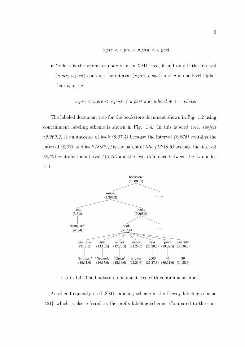
The labeled document tree for the bookstore document shown in Fig. 1.2 using

containment labeling scheme is shown in Fig. 1.4. In this labeled tree, subject

(2:269,2) is an ancestor of book (8:37,4) because the interval (2,269) contains the

interval (8,37), and book (8:37,4) is the parent of title (13:16,5) because the interval

(8,37) contains the interval (13,16) and the level difference between the two nodes

is 1.


bookstore

subject

name

“computer” book



……

……

subject

name book

title

“Network”

books

book

title

“Network”

author

book

title author

(t1) (t2)

bookstore(1:5000,1)

subject(2:269,2)

name(3:6,3)


book(8:37,4)

title(13:16,5)

author(17:20,5)

publisher(9:12,5)

year(25:28,5)

price(29:32,5)

quantity(33:36,5)

“Hillman”(10:11,6)

“Network”(14:15,6)

“Green”(18:19,6)

2003(26:27,6)

45(30:31,6)

30(34:35,6)

……

……

books(7:268,3)

bookstore(1)

subject(1.1)

name(1.1.1)


book(1.1.2.1)

title(1.1.2.1.2)

author(1.1.2.1.3)


year(1.1.2.1.4)

price(1.1.2.1.5)

quantity(1.1.2.1.6)

“Hillman”(1.1.2.1.1.1)

“Network”(1.1.2.1.2.1)

“Green”(1.1.2.1.3.1)

2003(1.1.2.1.4.1)

45(1.1.2.1.5.1)

30(1.1.2.1.6.1)

……

……

books(1.1.2)

post

5000

tag_name

bookstore

pre

1

level

1

value

null

post

5000

269

6

path

/bookstore

/bookstore/subject


pre

1

2

3




level

1

2

3

3

4

5

value

null

null

computer

null

null

Hillman

269

6

268

subject

name

books

2

3

7

33book 8

12publisher 9

...... ...

2

3

3

4

5

...

null

computer

null

null

Hillman

... ...... ... ... ...


bookstore

author

books

year

subject

name

book

publisher

bookstore (self_id)





dblp

article article ...

author


author

“John D. Musa”

title


pages

“85-170”

year

1990

volumn

30

journal



author

“Brown”

author(21:24,5)

“Brown”(22:23,6)

Figure 1.4: The bookstore document tree with containment labels

Another frequently used XML labeling scheme is the Dewey labeling scheme

[121], which is also referred as the prefix labeling scheme. Compared to the con-

10

tainment labeling scheme, the Dewey labeling scheme has advantage in finding the

lowest common ancestor of a few document nodes, which is a core operation for

XML keyword query processing. Thus the Dewey labeling scheme is widely adopted

in XML keyword search algorithms.

In the Dewey labeling scheme, the document root is assigned an initial ID, e.g.

1, and for any non-root node u, its Dewey ID is assigned by Dewey(u)=Dewey(v).x,

where u is the x -th child of node v. In other words, the Dewey ID of any document

node is its parent node’s Dewey ID appending a new component to indicate its

position among all siblings under the same parent node. Thus the level information

of each Dewey ID is implicitly represented by the number of components in it. The

document order, and PC and AD relationships are checked by Dewey IDs in such

a way that:

• Node u precedes node v in document order, if and only if Dewey(u) is lexi-

cographically precedes Dewey(v).

• Node u is an ancestor of node v in an XML tree, if and only if Dewey(u) is

a prefix of Dewey(v).

• Node u is a parent of node v in an XML tree, if and only if Dewey(u) is a

prefix of Dewey(v) and the number of components in u is one less than that

of v.

Fig. 1.5 shows the bookstore document tree with nodes labeled by the Dewey

labeling scheme. In this labeled tree, subject (1.1) is an ancestor of book (1.1.2.1)

because the Dewey ID 1.1 is a prefix of the Dewey ID 1.1.2.1 ; book (1.1.2.1) is the

parent of title (1.1.2.1.2) because 1.1.2.1 is a prefix of 1.1.2.1.2 and the difference

of number of components in the two Dewey IDs is 1; subject (1.1) is the LCA of

11


bookstore

subject

name

“computer” book



……

……

subject

name book

title

“Network”

books

book

title

“Network”

author

book

title author

(t1) (t2)

bookstore(1:5000,1)

subject(2:269,2)

name(3:6,3)


book(8:37,4)

title(13:16,5)

author(17:20,5)

publisher(9:12,5)

year(25:28,5)

price(29:32,5)

quantity(33:36,5)

“Hillman”(10:11,6)

“Network”(14:15,6)

“Green”(18:19,6)

2003(26:27,6)

45(30:31,6)

30(34:35,6)

……

……

books(7:268,3)

bookstore(1)

subject(1.1)

name(1.1.1)


book(1.1.2.1)

title(1.1.2.1.2)

author(1.1.2.1.3)


year(1.1.2.1.5)

price(1.1.2.1.6)

quantity(1.1.2.1.7)

“Hillman”(1.1.2.1.1.1)

“Network”(1.1.2.1.2.1)

“Green”(1.1.2.1.3.1)

2003(1.1.2.1.5.1)

45(1.1.2.1.6.1)

30(1.1.2.1.7.1)

……

……

books(1.1.2)

post

5000

tag_name

bookstore

pre

1

level

1

value

null

post

5000

269

6

path

/bookstore

/bookstore/subject


pre

1

2

3




level

1

2

3

3

4

5

value

null

null

computer

null

null

Hillman

269

6

268

subject

name

books

2

3

7

33book 8

12publisher 9

...... ...

2

3

3

4

5

...

null

computer

null

null

Hillman

... ...... ... ... ...


bookstore

author

books

year

subject

name

book

publisher

bookstore (self_id)





dblp

article article ...

author


author

“John D. Musa”

title


pages

“85-170”

year

1990

volumn

30

journal



author

“Brown”

author(21:24,5)

“Brown”(22:23,6)

author(1.1.2.1.4)

“Brown”(1.1.2.1.4.1)

Figure 1.5: The bookstore document tree with Dewey labels

computer (1.1.1.1) and book (1.1.2.1) because 1.1 is the longest common prefix of

1.1.1.1 and 1.1.2.1.

The Dewey labeling scheme has an advantage over the containment labeling

scheme in checking the LCA (lowest common ancestor) relationship between two

document nodes, which is widely used in XML keyword search. Since in this thesis

we focus on structured XML query, we do not illustrate how the labeling schemes

work for XML keyword search. Although both the two labeling schemes can be

used for twig pattern query processing, we choose to use the containment labeling

scheme in our demonstrations and experiments. This is because in the containment

labeling scheme, each label has a fixed size, which brings convenience in inverted

list management.

The containment labeling scheme and the Dewey labeling scheme are suitable

for static XML documents which are not updated. When the document is more

dynamic with updates, both schemes suffer from high cost of re-labeling. Recently,

several encoding schemes are proposed to transform the label format in each la-

12

beling scheme to a dynamic format, which is adaptive to updates. Such encoding

schemes include QED [78], Vector label [147] and DDE [150]. Apparently, the

containment labeling scheme used in this thesis can be enhanced by any dynamic

encoding schemes.

Labels are usually organized by inverted lists. Inverted list is an important data

structure widely adopted in XML twig pattern matching, XML keyword search, as

well as IR search. During XML twig pattern query processing, for each type of

document node (i.e., tag name or value), there is a corresponding inverted list to

store the labels of all nodes of this type in document order. To process a query, only

relevant inverted lists that correspond to the query nodes are scanned. Because

in most algorithms, each relevant inverted list is scanned in a streaming fashion

during query processing, inverted list in XML twig pattern query processing is

also referred as label stream, or simply stream. The update of the inverted list is

discussed in [15, 125, 19, 41].

1.4 Our research scope and contributions

Our research focuses on applying semantic information, such as value, property,

object and relationship among objects, to perform content search in structured

XML query processing. We put more focus on twig pattern query which is the

core pattern for structured queries as discussed in Section 1.2. Since we do not

emphasize on structural search, we use the basic twig pattern queries without

special structural predicates, e.g., OR predicate between edges, negation on edges

and wildcard nodes, for illustration. Those algorithms that perform structural joins

for these special predicates can be used for structural search in our approach, when

we extend our approach to support such special predicates.

13

Our contributions are summarized as:

1. We propose the VERT algorithm to efficiently perform both content search

and structural search during twig pattern query processing. The novelty of

VERT is to make use of the semantic information on object and property

to organize and query data values in XML documents. We observe that the

parent node of each value in an XML tree must be a property node, and value

predicate in queries is normally in form of property <operator> “value”. Thus

we introduce property-based relational tables to index each property node by

its value, and perform content search by selection in property tables. After

performing content search, a twig pattern query can be simplified by removing

value predicates, and some relevant inverted lists are reduced by the result

of content search. Then performing structural search on a simpler query

pattern with smaller inverted lists significantly improves the overall query

processing performance. In the last step, the relational tables can be used

to extract actual values based on returned labels, to answer queries. In this

way, we can eliminate redundant value answers though they may correspond

to different node labels. We also propose three optimizations when more

semantic information on object and relationship between objects is known.

Those semantic optimizations can further improve query processing efficiency.

Furthermore, we discuss how to use VERT to process queries across different

parts of an XML document by ID references or value-based joins, and queries

across multiple documents. Such a query is a bottleneck for many other

existing twig pattern matching algorithms, because they cannot link different

twig patterns by node labels.

2. We analyze the characteristics of each node in twig pattern query, i.e., the

purpose, optionality and occurrence, and classify the nodes in a twig pattern

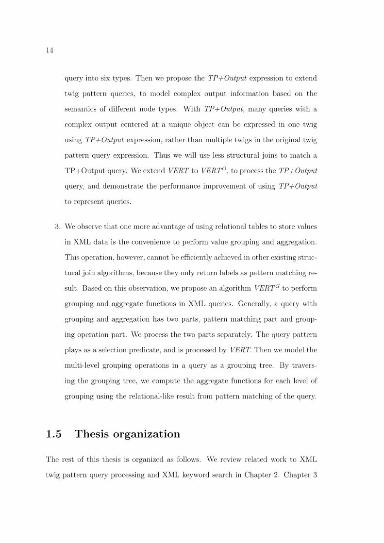
14

query into six types. Then we propose the TP+Output expression to extend

twig pattern queries, to model complex output information based on the

semantics of different node types. With TP+Output, many queries with a

complex output centered at a unique object can be expressed in one twig

using TP+Output expression, rather than multiple twigs in the original twig

pattern query expression. Thus we will use less structural joins to match a

TP+Output query. We extend VERT to VERTO, to process the TP+Output

query, and demonstrate the performance improvement of using TP+Output

to represent queries.

3. We observe that one more advantage of using relational tables to store values

in XML data is the convenience to perform value grouping and aggregation.

This operation, however, cannot be efficiently achieved in other existing struc-

tural join algorithms, because they only return labels as pattern matching re-

sult. Based on this observation, we propose an algorithm VERTG to perform

grouping and aggregate functions in XML queries. Generally, a query with

grouping and aggregation has two parts, pattern matching part and group-

ing operation part. We process the two parts separately. The query pattern

plays as a selection predicate, and is processed by VERT. Then we model the

multi-level grouping operations in a query as a grouping tree. By travers-

ing the grouping tree, we compute the aggregate functions for each level of

grouping using the relational-like result from pattern matching of the query.

1.5 Thesis organization

The rest of this thesis is organized as follows. We review related work to XML

twig pattern query processing and XML keyword search in Chapter 2. Chapter 3

15

presents the algorithm VERT, which use semantics-based tables to solve different

content problems in existing approaches, and to process twig pattern queries more

efficiently. We propose the twig pattern query extension, TP+Output, in Chapter

4, using which a subset of queries with complex output information centered at

one object can be easily expressed. An extended algorithm VERTO to process

TP+Output queries is also presented. In Chapter 5, we propose an algorithm

VERTG to physically perform grouping and aggregation in XML queries. Finally,

Chapter 6 concludes this thesis, and discusses some future research work.

16

CHAPTER 2

LITERATURE REVIEW

XML query processing has been studied for more than a decade. In this chapter, we

revisit existing research work on XML query processing. As mentioned in Chapter

1, XML data can be modeled as tree or graph, depending on whether the ID

reference is considered. We organize this chapter based on the tree model and

graph model of XML databases.

2.1 Query processing over XML tree

Twig pattern matching over tree-modeled XML data attracts the most research

interests in XML query processing. Generally, twig pattern matching algorithms

are categorized into two classes, the relational approach and the native approach.

They essentially differ on whether relational databases are used to store and query

XML data.

17

2.1.1 The relational approach

Relational model is a dominant model for structured data management. Over

decades, relational database management systems (RDBMS) have been well de-

veloped to store and to query structured data. As XML becomes more and more

popular, many researchers and organizations put more efforts into designing algo-

rithms to store and query semi-structured XML data using the mature RDBMS.

Generally, those relational approaches shred XML documents into relational ta-

bles and transform XML queries into SQL statements to query the database. The

advantage of the relational approach is that the existing query optimizer in the

RDBMS can be directly used to optimize the transformed XML queries. Espe-

cially for the queries with content search, the RDBMS can not only process the

value comparisons efficiently, but also push the value predicates ahead of table

joins using the optimizer. There are multiple shredding methods proposed for

the relational approach, which are classified into schemaless methods and schema-

based methods. The schemaless methods assume there is no schematic information

available, and decompose the XML document tree purely based on different tree

components. Typical schemaless methods include the node approach, the edge ap-

proach and the path approach. The schema-based methods decompose the XML

document tree based on schematic information, e.g., DTD. This kind of methods

require schema available alongside the document. Now we review the two kinds of

document decomposition methods and the corresponding query transformations in

more details.

Schemaless decomposition

Zhang et al. [156] proposed a node-based approach, which stores each document

node with its positional label into relational tables. The relationship between each

18

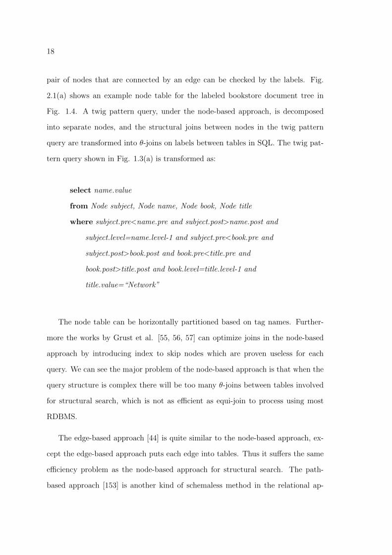
pair of nodes that are connected by an edge can be checked by the labels. Fig.

2.1(a) shows an example node table for the labeled bookstore document tree in

Fig. 1.4. A twig pattern query, under the node-based approach, is decomposed

into separate nodes, and the structural joins between nodes in the twig pattern

query are transformed into θ-joins on labels between tables in SQL. The twig pat-

tern query shown in Fig. 1.3(a) is transformed as:

select name.value

from Node subject, Node name, Node book, Node title

where subject.pre<name.pre and subject.post>name.post and

subject.level=name.level-1 and subject.pre<book.pre and

subject.post>book.post and book.pre<title.pre and

book.post>title.post and book.level=title.level-1 and

title.value=“Network”

The node table can be horizontally partitioned based on tag names. Further-

more the works by Grust et al. [55, 56, 57] can optimize joins in the node-based

approach by introducing index to skip nodes which are proven useless for each

query. We can see the major problem of the node-based approach is that when the

query structure is complex there will be too many θ-joins between tables involved

for structural search, which is not as efficient as equi-join to process using most

RDBMS.

The edge-based approach [44] is quite similar to the node-based approach, ex-

cept the edge-based approach puts each edge into tables. Thus it suffers the same

efficiency problem as the node-based approach for structural search. The path-

based approach [153] is another kind of schemaless method in the relational ap-

19


bookstore

subject

name

“computer” book



……

……

subject

name book

title

“Network”

books

book

title

“Network”

author

book

title author

join

(a) (b)

bookstore(1:5000,1)

subject(2:269,2)

name(3:6,3)


book(8:33,4)

title(13:16,5)

author(17:20,5)

publisher(9:12,5)

year(21:24,5)

price(25:28,5)

quantity(29:32,5)

“Hillman”(10:11,6)

“Network”(14:15,6)

“Green”(18:19,6)

2003(22:23,6)

45(26:27,6)

30(30:31,6)

……

……

books(7:268,3)

bookstore(1)

subject(1.1)

name(1.1.1)


book(1.1.2.1)

title(1.1.2.1.2)

author(1.1.2.1.3)


year(1.1.2.1.4)

price(1.1.2.1.5)

quantity(1.1.2.1.6)

“Hillman”(1.1.2.1.1.1)

“Network”(1.1.2.1.2.1)

“Green”(1.1.2.1.3.1)

2003(1.1.2.1.4.1)

45(1.1.2.1.5.1)

30(1.1.2.1.6.1)

……

……

books(1.1.2)

post

5000

tag_name

bookstore

pre

1

level

1

value

null

post

5000

269

6

path

/bookstore

/bookstore/subject


pre

1

2

3




level

1

2

3

3

4

5

value

null

null

computer

null

null

Hillman

269

6

268

subject

name

books

2

3

7

37book 8

12publisher 9

...... ...

2

3

3

4

5

...

null

computer

null

null

Hillman

... ...... ... ... ...

(a) A node table


bookstore

subject

name

“computer” book



……

……

subject

name book

title

“Network”

books

book

title

“Network”

author

book

title author

join

(a) (b)

bookstore(1:5000,1)

subject(2:269,2)

name(3:6,3)


book(8:33,4)

title(13:16,5)

author(17:20,5)

publisher(9:12,5)

year(21:24,5)

price(25:28,5)

quantity(29:32,5)

“Hillman”(10:11,6)

“Network”(14:15,6)

“Green”(18:19,6)

2003(22:23,6)

45(26:27,6)

30(30:31,6)

……

……

books(7:268,3)

bookstore(1)

subject(1.1)

name(1.1.1)


book(1.1.2.1)

title(1.1.2.1.2)

author(1.1.2.1.3)


year(1.1.2.1.4)

price(1.1.2.1.5)

quantity(1.1.2.1.6)

“Hillman”(1.1.2.1.1.1)

“Network”(1.1.2.1.2.1)

“Green”(1.1.2.1.3.1)

2003(1.1.2.1.4.1)

45(1.1.2.1.5.1)

30(1.1.2.1.6.1)

……

……

books(1.1.2)

post

5000

tag_name

bookstore

pre

1

level

1

value

null

post

5000

269

6

path

/bookstore

/bookstore/subject


pre

1

2

3




level

1

2

3

3

4

5

value

null

null

computer

null

null

Hillman

269

6

268

subject

name

books

2

3

7

33book 8

12publisher 9

...... ...

2

3

3

4

5

...

null

computer

null

null

Hillman

... ...... ... ... ...

(b) A path table

Figure 2.1: Example tables in node-based and path-based relational approaches

proach, which stores each path wholly without decomposition. One example path

table is shown in Fig. 2.1(b). The path-based approach saves table joins between

different nodes or edges along the same path, however, to perform a structural

search involving AD edge (“//”-axis), the path-based approach has to do a string

pattern matching (“LIKE” in SQL) on the path column, which is also an expensive

operation for relational database systems. Pal et al. [100] modified the path-based

approach by reversing the node positions in each path. By doing this, a twig pat-

tern query with AD edges can be decomposed into components beginning with

“//”, and “LIKE” pattern matching can be replaced by string prefix matching in

reversed paths, which is generally less expensive. There are also several works focus

on performing string prefix matching to improve efficiency, e.g., BLAS [28]. In the

last step, different components can be joined by the ORDPATH [99] label of each

path. This XML storage based on reversed path is used in Microsoft SQL Server.

Schema-based decomposition

When the schema of an XML document is known, the document can be shredded

based on the schematic information. Different from the schemaless methods, the

design of relational tables in the schema-based methods may vary for documents

with different schemas. Shanmugasundaram et al. [114, 113] proposed a DTD-

20

based approach to decompose XML documents. Consider the example shown in

Fig. 2.2. Based on the DTD, we can get a hierarchical structure between elements.

Then from the hierarchical structure, a set of relational tables are built. The

automatically generated attributes self id and parent id are the primary key and

foreign key of each table, which play as join attributes during query processing.


bookstore

subject

name

“computer” book



……

……

subject

name book

title

“Network”

books

book

title

“Network”

author

book

title author

join

(a) (b)

bookstore(1:5000,1)

subject(2:269,2)

name(3:6,3)


book(8:33,4)

title(13:16,5)

author(17:20,5)

publisher(9:12,5)

year(21:24,5)

price(25:28,5)

quantity(29:32,5)

“Hillman”(10:11,6)

“Network”(14:15,6)

“Green”(18:19,6)

2003(22:23,6)

45(26:27,6)

30(30:31,6)

……

……

books(7:268,3)

bookstore(1)

subject(1.1)

name(1.1.1)


book(1.1.2.1)

title(1.1.2.1.2)

author(1.1.2.1.3)


year(1.1.2.1.4)

price(1.1.2.1.5)

quantity(1.1.2.1.6)

“Hillman”(1.1.2.1.1.1)

“Network”(1.1.2.1.2.1)

“Green”(1.1.2.1.3.1)

2003(1.1.2.1.4.1)

45(1.1.2.1.5.1)

30(1.1.2.1.6.1)

……

……

books(1.1.2)

post

5000

tag_name

bookstore

pre

1

level

1

value

null

post

5000

269

6

path

/bookstore

/bookstore/subject


pre

1

2

3




level

1

2

3

3

4

5

value

null

null

computer

null

null

Hillman

269

6

268

subject

name

books

2

3

7

33book 8

12publisher 9

...... ...

2

3

3

4

5

...

null

computer

null

null

Hillman

... ...... ... ... ...


bookstore

author

books

year

subject

name

book

publisher

bookstore (self_id)





Figure 2.2: Example DTD, hierarchical structural between DTD elements, and therelations

Georgiadis et al. [48] enhanced the DTD-based approach by introducing an

additional relation to store path information, and proposed optimization [49] to

improve the efficiency of relational processor, as well as to accelerate XML recon-

struction from relational format. Some other similar schema-based decomposition

approach include [12, 36]. In particular, [36] discovers the schematic information,

i.e., the correlation between elements, by mining XML data.

A summary

Most relational approaches make use of existing relational query optimizers and

tune the system settings to get better performance for XML query processing.

Compared to the schemaless approaches, the schema-based relational approaches

is generally more efficient, as reported by [124].

Now we use to two real-life XML data, as shown in Fig. 2.3 to show the

advantage and the disadvantage of the relational approach. One major advantage

21

of the relational approach is the efficiency for content search in a query. All value

comparisons in query predicates are eventually transformed into table selection,

which can be efficiently evaluated under the help of B+ tree index of the RDBMS.

Thus, the relational approach is suitable for regular XML data, such as DBLP [35]

data which is partially shown in Fig. 2.3(a). Queries over such data normally have

simple structural constraints, but focus more on content search.

However, some XML data are rather deep and complex in structure. For ex-

ample, the TreeBank [97] data (a partial document is shown in Fig. 2.3(b)) has a

maximum depth of 36 and an average depth of 8, and contains a lot of recursive

tags. Queries to such a deep and complex document may also contains complex

structures, which require many steps of expensive table joins for structural search.

Furthermore, the schema-based approach cannot efficiently handle AD edges (“//”)

in queries to such a document with recursive tags. Consider a query edge VP//PP

to be matched in the TreeBank data. The schema-based approach can hardly de-

cide what tables to be joined between VP and PP and how many times to join

them. Krishnamurthy et al. [76] proposed to use structural labels (e.g., contain-

ment labels) as keys of each table, which can handle AD edges. In more details, for

each “//”-axis join, they join the two tables based on labels to check AD relation-

ship, which is the same as what the node approach does. However, transforming

equi-join based on primary key and foreign key to θ-join on labels seriously affects

the performance because most RDBMS cannot perform θ-join as efficiently as equi-

join. There are also some other work to handle recursive elements during query

transformation, e.g., [75]. Similarly, they also suffer from efficiency problems dur-

ing query processing. Structural join based native approach is much more efficient

than the relational approach for such queries and data, which will be reviewed in

the next section.

22


bookstore

subject

name

“computer” book



……

……

subject

name book

title

“Network”

books

book

title

“Network”

author

book

title author

join

(a) (b)

bookstore(1:5000,1)

subject(2:269,2)

name(3:6,3)


book(8:33,4)

title(13:16,5)

author(17:20,5)

publisher(9:12,5)

year(21:24,5)

price(25:28,5)

quantity(29:32,5)

“Hillman”(10:11,6)

“Network”(14:15,6)

“Green”(18:19,6)

2003(22:23,6)

45(26:27,6)

30(30:31,6)

……

……

books(7:268,3)

bookstore(1)

subject(1.1)

name(1.1.1)


book(1.1.2.1)

title(1.1.2.1.2)

author(1.1.2.1.3)


year(1.1.2.1.4)

price(1.1.2.1.5)

quantity(1.1.2.1.6)

“Hillman”(1.1.2.1.1.1)

“Network”(1.1.2.1.2.1)

“Green”(1.1.2.1.3.1)

2003(1.1.2.1.4.1)

45(1.1.2.1.5.1)

30(1.1.2.1.6.1)

……

……

books(1.1.2)

post

5000

tag_name

bookstore

pre

1

level

1

value

null

post

5000

269

6

path

/bookstore

/bookstore/subject


pre

1

2

3




level

1

2

3

3

4

5

value

null

null

computer

null

null

Hillman

269

6

268

subject

name

books

2

3

7

33book 8

12publisher 9

...... ...

2

3

3

4

5

...

null

computer

null

null

Hillman

... ...... ... ... ...


bookstore

author

books

year

subject

name

book

publisher

bookstore (self_id)





dblp

article article ...

author


author

“John D. Musa”

title


pages

“85-170”

year

1990

volumn

30

journal


(a) DBLP data

S

VP NP

PP

NP

PP

NP

VP

S

… …

…

(b) TreeBank data

Figure 2.3: Two real-life (partial) documents with different characteristics

2.1.2 The native approach

To improve the performance of structural search in XML queries, many native

approaches are proposed. In the native approach, documents are not stored using

relational tables, thus the overhead on table join to perform structural search can

be avoided.

Structural join approach

The structural join approach is a very important class of native approach that

attracts most research interest. In this sort of approach, a document is pre-parsed

by assigning a label to each document node. Then the labels for each type of

document node are organized using an inverted list (or called stream), in document

order. The details of document labeling and inverted lists were discussed in Section

1.3. A twig pattern query is processed by scanning the relevant inverted lists to

23

find the matched documents nodes.

Binary join

In the early work, Zhang et al. [156] proposed the multi-predicate merge join

algorithm. In their approach, the twig pattern query is decomposed into multiple

binary joins. The query is processed by finding all matched node pairs to each

binary join, and combining these binary matches. When they match a binary join,

e.g., A/B (or A//B), they scan the inverted lists for the node type A and B. For

each pair of labels in the two inverted lists they check whether they are satisfied

with parent-child (or ancestor-descendant) relationship. Because the labels in each

inverted list are sorted by the document order, this process can be implemented

efficiently, which is quite similar to the merge-join in relational systems. However,

this technique suffers from the efficiency problem of unnecessary checking of labels

in inverted lists, as pointed out by Al-Khalifa et al [1]. Then in [1] they improved

the binary join approach by adding a stack to cache the nested nodes so that the

unnecessary label checking can be avoided. This stack-based binary join algorithm

is also adopted by the native XML database, TIMBER [62]. There are also several

indices built on inverted list to accelerate label scans for structural join processing

[33, 65].

The major problem of the binary join approach is the large size of useless

intermediate results produced by binary joins, when the query plan is not well

chosen. Once we perform the binary join with very low selectivity first, many

intermediate matches may be useless for final result. This also motivated some

work on structural join order selection [145].

Holistic join

24

Bruno et al. proposed TwigStack [16], which is a holistic join approach to avoid

producing too many useless intermediate results. Comparing to the binary join

approach, the major difference is that TwigStack introduces multiple stacks for

all the query nodes and scanning multiple inverted lists at one time, to find the

matched patterns. TwigStack first produces the matched paths that contribute to

the final result, and then merges the matched paths to twigs. They introduce a

getNext function to ensure that each matched path is useful in later merging pass,

when the path contains only AD relationships. In this point of view, TwigStack is

optimal for twig pattern queries with only AD relationships.

There are many subsequent works [83, 66, 45, 26, 85, 64, 155] to optimize

TwigStack in terms of I/O, or extend TwigStack to solve different kinds of problems.

In particular, Lu et al. [83] introduced a list structure to make it optimal for queries

containing parent-child relationships between non-branching nodes. TSGeneric [66]

improved the query performance based on indexing each inverted list and skipping

labels within one inverted list. Fontoura et al. [45] further optimize the cursor move

in inverted lists to reduce cost. Chen et al. [26] divided one inverted list into several

sub-lists associated to each prefix path or each (tag, level) pair and pruned some

sub-lists before evaluating the twig pattern. Lu et al. [85] used Extended Dewey

labeling scheme and scanned only the labels of leaf nodes in a twig query. [64] and

[155] extended twig pattern query to support OR-predicate and NOT-predicate

respectively.

Besides, Twig2Stack [25] proposed a bottom-up strategy to evaluate twig pat-

tern queries using nested stacks. It is worst-case optimal, and is also capable to

process queries with optional edges. Some later work [67, 104, 79] use improved

evaluation strategy and data structure to achieve better performance for practical

queries, though they are not optimal for the worst cases. Recently, Grimsmo et al.

25

[54] proposed to use a similar data structure to those in [104, 79] to achieve worse-

case optimal time without scarifying performance for practical queries. Shalem

et al. [112] discussed the space usage of twig pattern matching, and proposed a

query-driven technique to avoid some overhead. The optimality of twig pattern

matching is theoretically studied in [84].

Graphic index

Graphic index is a useful tool to accelerate query processing with the structural

join based approaches. A graph index normally covers all path or twig patterns in

an XML document, so that when a query is contained in a graphic index, the query

processor could return the matching results directly, without performing (or per-

forming less) structural joins. The graphic indexes are categorized into two classes:

path index and twig index.

Strong DataGuides [51] is an early path index which could cover all path in-

formation. However, Strong DataGuides is too large comparing with the target

document. Later 1-index [92], A(k)-index [71] are proposed to reduce the index

size based on backward bisimilarity and k-bisimilarity. To process a twig pattern

query using a path index, the twig pattern is first decomposed into paths. Af-

ter finding the intermediate results for each path, the final result is generated by

joining these intermediate results based on the positional relationships of paths.

Twig index is the other class of graphic index, which covers all twig patterns in

the given XML document. One famous twig index is the F&B index [69, 105], which

is also proven the smallest index to cover all twig patterns for any XML document

[69]. Using F&B index, the twig pattern queries with only PC relationships can

be processed by searching the index to return the answers, instead of performing

structural joins. However, sometimes F&B index is still too large to fit in memory.

26

Wang et al. proposed a disk-based organization [133] for F&B index. Intuitively,

to process a twig pattern query using F&B index involves the traversal of the F&B

index, which is non-deterministic as pointed by [133]. When the query also contains

“//”-axis, the searching becomes more complex. In [133], they combine the F&B

index with other structural join based native approach, e.g., TwigStack, to process

queries. They decomposed the twig pattern query by “//”-axis. For each part that

contains only “/”-axis, they use the disk-based F&B index to find the intermediate

results in terms of node labels, and then use TwigStack with the intermediate node

label streams to handle the “//”-axis. In this way, the structural search becomes

more efficient. Recently, Tang et al. [118] proposed an indexing technique that can

cover twig patterns containing both “/”-axis and “//”-axis.

Other native approaches

The subsequence matching approach is another class of native approach. PRIX

[106] and ViST [132] transform both XML documents and queries into sequences

and perform subsequence matching between query sequence (as subsequence) and

document sequence. In particular, ViST derives document sequence based on pre-

order document traversal, while PRIX makes use of Prufer sequences which are

derived from post-order traversal. Tatikonda et al. [122] employed a dynamic pro-

gramming based technique to perform subsequence matching. Moro et al. [124]

conducted experiments to show that the subsequence matching approach is nor-

mally not efficient and robust as the structural join approach.

Besides the structural join approach and the subsequence matching approach,

there are also a number of algorithms which scan an XML document to find the

occurrences of queries. We name this sort of approach navigational approach. A

direct navigational approach is to read an XML document with a certain API,

27

e.g., SAX parser [110], and check the events generated by SAX based on query

constraints. Some applications, e.g., [50], use this direct approach to match a query

pattern to a document. However, this naive approach can only process simple twig

pattern queries without recursive nodes. When a query involves recursive nodes,

they have to use stacks to store SAX events [11], which is similar to the structural

join approach.

The navigational approach for query processing is widely adopted by differ-

ent native XML storages. In some early native XML database systems [90, 43],

documents are normally partitioned into pieces to store on disk, and queries are

processed by navigating relevant disk pages. Buneman et al. [17] summarized an

XML document as a skeleton (similar to the DataGuides index), and clustered the

values under each kind of document path together. They traversed the skeleton

and load relevant values to process queries. In [59] and [158], the authors argued

that navigating a proper XML storage is more efficient than structural join to pro-

cess “/” axis in queries. Motivated on this, they proposed to decompose a twig

pattern query based on “//” axis, so that every component only contains edges of

“/” axis. Each component is matched by navigating the native XML storage, and

structural join is used to solve the “//” axis between components. Wong et al.

[135] proposed a compact XML storage and a way to perform relevant navigational

operations over their storage. The navigational approach is also used in querying

XML streams [103, 68, 29, 8].

Generally, both the subsequence matching approach and the navigational ap-

proach need to scan a large portion of (or whole) XML document during query

processing. This attempt leads a high I/O cost. In contrast, the structural join

approach only reads the inverted lists which are relevant to the query nodes to pro-

cess a query. Thus it normally introduces lower I/O cost. Also, there are several

28

techniques, e.g., selective index [60] and materialized view [4, 87, 151, 2, 119, 23],

to maintain cache for frequently asked (sub-)query pattern in the structural join

approach. All these factors make the structural join approach a representative

native approach.

2.1.3 Comparison between the relational approach and the

native approach

Both the relational approach and the native approach to process XML queries

have their own advantages and disadvantages. In relational approach, the values

in an XML document can be efficiently managed using relational tables. Also

both the content search and the value extraction for final answer can be easily

performed by SQL selection. However, though there are different methods to shred

XML data into tables, all of them suffer from problems in performing structural

search, especially for handling “//” axis. The native approach is a good choice

for structural search. However, the native approach cannot perform content search

efficiently, and cannot extract values to answer the query using the inverted list

index. The details of these problems regarding values in the native approach are

discussed in Section 3.1.

It is not easy to generally comment on which kind of approach is better in query

processing performance, because both approaches have a number of variants, and

both approaches may employ different indexes to speed up query processing. In

some preliminary reports, Zhang et al. [156] conducted experiments to show a

binary join based native approach is better than a node based relational approach.

Kurt et al. [77] showed the relational approach is faster than the native approach

for data-centric XML documents. Chaudhri et al. [22] concluded that the native

approach is suitable for large data sets and the relational approach is good for

29

smaller data sets (though they did not mention the concrete size). However, all

the comparisons are done by particular implementations of the relational approach

and the native approach and conducted under particular environments (hardware,

database parameter, indexing, etc). As mentioned by Serna et al. [111], actually

there is no tool feasible to analyze whether XML data should be queried natively

or using RDBMS, to get a better performance.

Although it is hard to compare the two approaches, the advantages and limi-

tations of the two approaches are obvious. It will be interesting to find a way to

combine the advantages of the relational approach and the native approach, and

avoid the limitations.

2.1.4 Hybrid management of relational data and XML data

In the early stage, most XML-enabled relational database systems used the rela-

tional approach to process XML queries, and most native XML database systems

used the native approach. As both the relational format and the XML format

have become very important in data storage and exchange, many database vendors

extended their systems to be hybrid for both relational data and XML data. We

take Oracle 11g, Microsoft SQL Server, and IBM DB2 to show how these database

systems manage XML data in a hybrid platform.

In the prior versions of Oracle database systems, XML data is either stored as a

CLOB column or shredded into object-relational tables based on their schema. In

Oracle 11g [82, 157], a new binary storage is introduced. This is a native storage for

XML data. When they process an XML query, the query is first rewritten to their

SQL-like syntax with Oracle operators. Then the processor scan the binary XML

input stream to find the query answers. The whole process of query processing is

a navigational native approach.

30

Microsoft SQL Server 2000 [108] shredded XML data into relational tables to

manage and query. Later, in SQL Server 2005 [109], they developed a native BLOB

storage for XML data. However, besides the native XML storage, they also use

relational tables to index each path. During XML query processing, they actually

searched the relational tables [100, 99]. Thus with respect to query processing, the

technique in Microsoft SQL Server is actually a relational approach.

IBM DB2 used the System RX [11] to store and query relational data and XML

data separately. For XML storage, they invented a column type of XML, which

is similar to the Oracle database. An XML document is stored natively as a tree

model under each XML-typed entry. During query processing, they traversed the

XML document to find query matches, under the help of different indexes. Actually

this attempt is also a navigational native approach.

The concept of “hybrid” in Oracle, SQL Server and DB2 means they manage

both relational and XML data in a single system. However, when they process XML

queries, they adopt either a pure relational approach or a pure native approach.

Our approach, which is presented later, incorporates both relational tables and

native inverted lists to aid query processing. This is a hybrid attempt w.r.t. query

processing, to effectively inherit the advantages of the relational approach and the

native approach, and avoid the problems of these two kinds of approaches.

2.2 Query processing over XML graph

When we consider the ID references in an XML document, the document should

be modeled as a graph, rather than a tree. Similarly, when a query involves ID

references, it is not in a twig pattern, but in a graph pattern. How to match a

graph pattern query to an XML graph is essential to XML query processing with

31

ID references. The relational approach for twig pattern matching, reviewed in the

previous section, can be used for XML graph matching. However, as indicated

previously, the efficiency problem caused by the overhead on table joins becomes a

major concern for the relational approach. In this section, we focus on the existing

works of native graph matching, without using RDBMS.

The initial attempt for XML graph matching is to check subgraph isomorphism,

which is a classic mathematical problem and is widely adopted in graph databases.

For example, the approach proposed in [115] generated all possible mappings be-

tween each pair of nodes in two graphs and check for correctness. Generally, this

sort of graph matching problem is NP-complete [47]. There are also many indices

proposed on graph database to reduce the complexity of subgraph isomorphism

checking [152, 159, 31, 134, 160, 61]. However, subgraph isomorphism checking

is only suitable for matching a graph pattern XML query without AD relation-

ships. There is another class of research problems in graph databases that focus

on connectivity-based pattern matching [32, 126, 161]. Theoretically, they can be

modified to match a graph pattern query to an XML graph by setting a distance

constraint between the two nodes connected by a PC or AD edge in the query.

However, all these attempts focused on random graph databases and did not cap-

ture the characteristics of XML queries. In an XML query, the edge between two

adjacent nodes can only be “/” or “//”, which specify the distance between them

is either 1 or unlimited. Applying the general subgraph matching algorithms to

XML graph matching may not be efficient as expected. There is a need to design

specific algorithms based on the characteristics of XML data, to perform XML

queries involving ID references.

Chen et al. [24] extended TwigStack, which is used for twig pattern matching,

to process graph matching for XML data and queries involving ID references. They

32

assumed the XML data to be DAGs (Directed Acyclic Graphs), and maintain an

index to store positional relationships between nodes. Each time they process a

query, partial solutions are expanded based on the index. Although they showed

that their approach was more efficient than a traditional graph matching algorithm

[115], compared with other structural join based algorithms for XML query pro-

cessing, their algorithm was still very slow. Similarly, Vagena et al. [127] proposed

another algorithm to match graph pattern queries on XML DAGs. The major

problem of these DAG-based matching algorithms is that an XML document with

ID references may form cycles. When they handle such cyclic XML documents,

they may generate a large number of results that contribute to the same valuable

information [74]. Recently, Wang et al. [131] proposed a new labeling scheme for

document graph so that PC and AD relationships between two graph nodes can

be identified based on their labeling scheme, and then queries can be processed by

structural joins. However, this approach, as well as the DAG-based approaches,

only paid attention to the characteristics of XML queries, but did not notice the

semantics of ID references in both data and queries, which is that an ID reference

always starts from an IDREF attribute and points to an object with the same

ID value. In Chapter 3, we will demonstrate that our semantic approach can re-

duce graph matching to less complex tree matching by using the semantics of ID

reference.

2.3 Summary of related work

In this chapter, we review the related work on XML query processing. We start

from the case that queries are issued over tree-modeled XML data. In this case,

we can model the queries as twig patterns, which is also a tree structure. There

33

are two classes of approaches to match a twig pattern query to an XML document,

namely the relational approach and the native approaches.

The relational approach use the RDBMS to store XML documents, and convert

queries into SQL statements to query the tables. There are two types of decom-

position methods to shred an XML document into relational tables. The first type

is the schemaless decomposition, which creates tables and shreds documents based

on structural components of a document tree, i.e. node, edge or path. The sec-

ond type is the schema-based decomposition, which shreds documents based on

schematic information, e.g., DTD. Generally, the schema-based decomposition is

more efficient than the schemaless decomposition to process queries, but it requires

schematic information that may not be available for any XML documents.

The native approach to process XML twig pattern queries attracts more interest

in recent research. The native approach can be divided into the navigational ap-

proach, the subsequence matching approach and the structural join approach. The

structural join approach uses inverted lists to organize document nodes (in terms of

labels), thus avoids the high I/O cost to scan irrelevant parts of a document. This

makes the structural join approach more efficient than the other two approaches

generally. The state-of-the-art structural join approach is based on holistic struc-

tural join, which performs structural joins in a holistic view. This attempt controls

the size of useless intermediate result, thus results in a better query performance.

The comparison of different approaches to process XML twig pattern queries,

w.r.t. the efficiency in structural search and content search, is shown in Fig. 2.4.

We can see different existing approaches suffer from efficiency problems in either

structural search and content search. Our approach can perform both types of

searches efficiently.

Last, we review the research works on the XML query processing over graph-

34

Different approachesstructural search

Relational approaches

weak

weak

content search

good

good

Schemaless

Schema-based

Native approaches

medium

medium

weak

weak

Navigational

Subsequence matching

Two types of searches

good weakStructural join based

Our approach good good

Figure 2.4: Comparison of approaches to process twig pattern query processing

modeled XML data, i.e., the data with ID references under consideration. Gener-

ally, the relational approach can be adopted to process graph pattern matching,

however, the inefficiency of multiple rounds of table joins becomes a main limita-

tion. There are two ways to perform pattern matching natively in graph-modeled

XML data. The first way is to modify the graph isomorphism checking or graph

pattern matching algorithms in general graph databases to process XML queries.

However, an XML graph is not as complex as a random graph and an XML queries

only contains edges of two types (i.e., PC edge and AD edge). Using the algo-

rithms in general graph matching may not be efficient as expected to process XML

queries. The second way to perform XML graph pattern matching is to extend

the structural join algorithms in twig pattern matching. The relevant approaches

either maintain index to record additional edges on top of tree structure (to form a

graph) for the XML data, or invent new labeling scheme for XML graphs. We argue

that graph pattern matching is generally more complex than twig (tree) pattern

matching. If we can capture the semantics of ID reference, we may reduce graph

matching to tree matching to process queries over XML data with ID references.

35

CHAPTER 3

A SEMANTIC APPROACH FOR TWIG

PATTERN QUERY PROCESSING

As introduced in Chapter 1, a twig pattern query includes structural search and

content search. Existing approaches to process XML twig pattern queries suffer

from problems in either structural search or content search. In this chapter, we

present our work which adopts a semantic approach to process XML twig pattern

queries. Briefly, our approach introduces both semantics-based relational tables

and inverted lists to aid query processing. The structural search and the content

search in a twig pattern query are performed with inverted lists and relational tables

separately. We show that this hybrid approach can achieve better performance in

both searches. Moreover, using relational tables to store values and perform content

search, our algorithm can easily process queries involving ID reference and more

general queries containing multiple twig patterns linked by value-based joins.

Furthermore, relational tables in our approach are initially constructed based

36

on the default semantics, i.e., the relationship between property and value, which

can be discovered in any XML documents. Later, as more semantics on object

and relationship between objects is known, we further optimize the tables accord-

ingly. We demonstrate that using the optimized tables, we can process twig pattern

queries more efficiently.

Last, we conduct experiments to show the benefit of our approach, by comparing

with existing approaches.

3.1 Introduction and motivation

Twig pattern is the core pattern for XML queries, as introduced in Chapter 1.

Existing twig pattern query processing approaches are classified into relational

approaches and native approaches. Both approaches have their own advantages and

disadvantages in performing the structural search and the content search in a twig

pattern query. In Chapter 2, we illustrate the problems of relational approaches to

handle structural search. In this section, we discuss the problems of a representative

native approach in dealing with values in XML documents, which motivate our

research in this chapter.

The structural join based approach is the state-of-the-art approach in XML twig

pattern query processing. It is proven more efficient than relational approaches

and other native approaches generally. However, because they do not differenti-

ate the semantics of value and other types of document nodes (i.e., elements and

attributes), they suffer from several problems related to values during query pro-

cessing. Now we illustrate the problems caused by ignoring value semantics.

1. Inverted list management. In most structural join based approaches, all

the nodes including elements, attributes and values in an XML tree are labeled

37

and the labels of each type of nodes are organized in an inverted list. When

we build inverted lists for values, the management is a problem. Consider

the bookstore document with every node labeled as shown in Fig. 1.1. There

are a large number of books and each of them probably has a different title.

In this case we have to maintain an inverted list for each different title value,

e.g., ‘Network’, ‘Database’ and so on. Based on our investigation, a 100MB

XML document contains around 4 million different values, which correspond

to 4 million inverted lists1. This number will linearly increase according to the

document size. To manage the tremendous number of inverted lists becomes

a problem.

2. Advanced content search. Twig pattern queries normally models XPath

expressions. Thus the advanced content search, such as numeric range search,

containment search or even conjunction/disjunction of several value compar-

isons, which often appear in XPath query predicates, may also appear as a

leaf node in a twig pattern query. Without handling values specially, existing

approaches have difficulty in supporting these advanced content search. For

example, to process a query to find the books with price less than 50, it is

time consuming to get all the inverted lists with numeric names which are

less than 50, and combine labels in them by document order, to perform this

range search. Also for the query //book[contains(@title, ‘XML query’)]/price

to find the price of the book that contains ‘XML query’ in its title, using in-

verted lists to index title values can hardly support such containment search

efficiently.

1Different from the inverted lists used in IR search and XML keyword search which index everysingle keyword, inverted list used in existing twig pattern query processing algorithms indexesa whole value so that the structural join between this value and other types of nodes can beperformed with the corresponding inverted lists.

38

3. Redundant search in inverted lists. Inverted lists for values do not have

semantic meanings. This may cause redundant search during inverted list

scanning. For example, When a query is interested in the books with price

of 35 in the bookstore document, structural search scans the inverted list

for value node ‘35’ (denoted by T35). Since in T35 we do not differentiate

whether a label corresponds to price or quantity, we need check all the labels

in this inverted list though many of them stand for quantity equals to 35, and

definitely do not contribute to the query result.

4. Actual value extraction. When we issue a query to an XML document,

what we need is not all the twig pattern occurrences represented as tuples

of labels, but the value results of that query. For example, after finding a

number of occurrences of the twig pattern query in Fig. 1.3(a), we need to

know the value under each name node. One major advantage of the structural

join based approaches is that they only need to load the relevant inverted lists

to process the query, instead of scanning the whole document with high I/O

cost in other approaches. However, after getting a set of resulting labels from

pattern matching, they cannot find the child value under each label using

inverted lists. To extract actual values, they have to read the document

again, which violates the initial will in I/O saving.

Motivated on solving all these problems, we propose a semantic approach that

uses both inverted lists and relational tables to perform twig pattern matching. In

particular, relational tables are used to store values, while inverted lists are used

to index internal document nodes, including property nodes and object nodes.

We propose the VERT algorithm to perform content search and structural search

separately with the two kinds of indexes in twig pattern matching. Content search

is performed by table selection before structural search. Because content search

39

is always a predicate between a property and a value, after performing content

search the size of the inverted list of the relevant property node is reduced due

to the selectivity of the predicate, and the twig pattern query can be simplified

by removing value comparisons. Matching a simplified twig pattern with reduced

inverted lists for several query nodes will reduce the complexity of structural search,

and thus improve the twig pattern matching performance. Finally, the semantic

table can help to extract actual values to answer the query, if the query output is a

property node (property node is discussed below) which appears in most practical

XML queries. Whereas, it is not efficient to extract child values of node labels in

other structural join based approaches.

We also need to highlight that the relational tables are constructed based on se-

mantic information such as value, property, object and relationship among objects.

The semantics of property is apparent for any XML document, i.e., the parent node

of each value must be the property of that value. Based on this default seman-

tic information, we initially store each value with the label of its property in the

corresponding relational table. With more semantics on object, we propose three

optimization techniques to change the tables to be object based. We will show that

using object-based tables, a query can be processed even more efficiently.

The rest of this chapter is organized as follows. We present the main algorithm

of VERT in Section 3.2. In Section 3.3 we describe how we optimize tables, as well

as query processing with more semantic information. We discuss how to extend

VERT to process general XML queries across multiple twig patterns in Section

3.4. We present the experimental results in Section 3.5 and summarize this work

in Section 3.6.

40

3.2 VERT algorithm

In this section, we present our algorithm VERT, to efficiently process XML twig

pattern queries. We introduce relational tables as an index to help to perform

content search and value extraction. Our approach is a semantic approach because

the relational tables are built based on semantic information such as property,

object, and relationship among objects. We first discuss the semantics of object

and property, and then move to our main algorithm.

3.2.1 Object-related semantics in XML data

Object (or entity) is an important information unit in database management, such

as the ER approach to design a relational database. In XML databases, object also

plays an important role, as most XML queries ask about information of certain

objects. An object may have several properties to describe the object from different

aspects. The property is also referred as attribute. To differentiate it from attribute

type in document schema (e.g., DTD), we use the term property in this thesis.

The semantics of object and property in XML data is actually apparent. If

a user does not know how objects are organized in an XML document, he can-

not compose any structured query, e.g., XPath or XQuery query to search the

database. For example, a user wants to find the title of the book written by

“White” in the two documents designed differently in Fig. 3.1 (partially shown).

No matter how the document is designed, the user has to know that the book

node is the object he wants to find, though the book node is not directly con-

necting the author node in the two documents. Knowing this, he will issue the

query //book[authors/author=“White”]/title to the first document and the query

//book/basicInfo[author=“White”]/title to the second document. Although se-

41

mantics is important in query composing, very few work paid attention to use such

semantic information to improve query processing performance.

In our approach, we make use of such semantics as object and property to aid

twig pattern query processing. In an XML document tree, value nodes must appear

as tree leaves. The parent node of each value node must be a property node with

the corresponding value. For example, publisher, title, author, price and quantity

are all properties in the bookstore document, because they are parent nodes of

values. An object node sometimes appears as the parent node of some property

nodes. For example, in the document in Fig. 3.3, every subject and every book

are all objects, and they are parent nodes of properties such as name, publisher,

title, etc. However, in some documents, the properties do not directly follow their

objects. For example, if the document further groups the properties of a book as

shown in the two examples in Fig. 3.1, the parent node of a property, i.e., authors,

basicInfo or saleInfo, is not an object.

book

title

author

publisher price quantity

“Elco” “Database”

“White”

35 15author

“Brown”

authors

book

title authorpublisher price quantity

“Elco” “Database” “White” 35 15

author

“Brown”

basicInfo saleInfo

Figure 3.1: Two alternative design of book in the bookstore document

Two or more objects that are related to each other normally reside along the

same path in an XML tree. However, the properties of a relationship may be

misunderstood with object properties, due to the hierarchical structure of XML

data. Consider the document design in Fig. 3.10. Quantity is a property of

the relationship between branch and book, but this property appears as a child

42

node of book, in the same way as other book properties. Although simply from

the document tree (or even DTD or XML Schema) we cannot tell the difference

between relationship property and object property, in fact, this information must

be known beforehand. Actually, a user’s awareness of the semantic meaning of

each document node is not bound to the structure of the document. As mentioned

above, a user must always be aware of such semantics in order to compose a correct

XPath or XQuery query based on his search intention.

In case such semantic information is not available, there are also many attempts

to discover the semantics such as object and relationship between objects in an

XML document. Generally, there are categorized into three classes.

1. Using available tools and information. There are semantic rich models that

work as a schema for XML documents. For example, ORA-SS [80] model can

distinguish between properties, objects and relationships, as well as specify

the degree of n-ary relationships and indicate if a property belongs to an ob-

ject or a relationship. If such model is available alongside an XML document,

we can easily discover useful semantic information. Also as semantic web is

rapidly developed, there are many ontologies available for different domains.

By exploring the ontology of relevant domains, we can have desired semantic

information of an XML document.

2. Mining schema or document. Liu et al. [81] infer objects by analyzing DTD,

though it is not very precise. [27] and [154] propose algorithms to discover

the semantics such as keys and functional dependencies in XML documents,

which can help to identify objects and relationships. There are also many data

mining techniques, such as decision tree, can be adopted to infer semantic

information.

43

3. User interaction. In many web-based information management systems [39][116],

they use mass collaboration to seek for feedback from users to improve se-

mantics identification.

In our work, we use known semantics on value, property, object and relationship

among objects to design our algorithms.

3.2.2 An overview of VERT

In VERT, we pay attention to values during index construction. We maintain

inverted list index only for structural nodes (non-valued nodes). For each value

node, we store it into the relational table index2 with the label of its property

node, instead of labeling it and putting its label into an inverted list as other

approaches do. Now, the number of inverted lists is limited to the number of

different element/attribute types in the document.

Query processing in VERT includes three steps. In the first step, we perform

content search for the value comparisons in query predicates, using relational ta-

bles. After that, the query is rewritten by removing all value comparisons. In the

second step, we perform structural search for the simplified query pattern, using

any structural join algorithms, e.g., TwigStack [16]. The last step is to extract

values to answer the query from the relational tables. Fig. 3.2 shows the general

process of query processing with VERT.

2To avoid the overhead on maintaining relational tables, the relational table index can also bereplaced by other types of index to bidirectional map values and their properties. However, thetrade-off is the inconvenience to support advanced content search and to meet the requirementsin our object-related optimizations.

44

bookstore(1:5000,1)

subject(2:307,2)

name(3:6,3)


book(8:29,4)

title(13:16,5)

author(17:20,5)

publisher(9:12,5)

price(21:24,5)

quantity(25:28,5)

“Hillman”(10:11,6)

“Network”(14:15,6)

“Green”(18:19,6)

45(22:23,6)

30(26:27,6)

……

……

subject

name book

title

“Network”

books(7:306,3)

book(30:55,4)

title(35:38,5)

author(39:42,5)

publisher(31:34,5)

price(47:50,5)

quantity(51:54,5)

“Elco”(32:33,6)

“Database”(36:37,6)

“White”(40:41,6)

35(48:49,6)

15(52:53,6)

author(43:46,5)

“Brown”(44:45,6)

book

title

“Network”

author

book

title

join

(a) (b)

Content Search

Query RewrittingQuery Step 1 Structural

SearchStep 2 Output Value

ExtractionStep 3

Inverted lists for element nodes

Relational tables for value nodes

Figure 3.2: Overview of VERT

3.2.3 Document parsing in VERT

When we parse an XML document, we only label elements and attributes, and

put the labels into corresponding inverted lists in document order. Values in the

document are not labeled, instead we put them into relational tables together with

labels of their parent property nodes. Normally this parsing step is only executed

once for an XML document, and after all relevant indexes are properly built during

the parsing step, the system is ready to process any twig pattern queries over the

given document. The detailed algorithm Parser is presented in Algorithm 3.1.

We use the SAX to read the input document and transform each tag and value

into events. Line 3 captures the next event if there are more events in the SAX

stream. Based on different types of events, different operations are performed

accordingly. Line 4-16 are executed if the event e is a start tag. In this case, the

first two steps are triggered. The system first constructs an object for this element

and assigns a label to it. It then puts the label into the inverted list for that tag. A

stack S is used to temporarily store the object so that when an end tag is reached,

the system can easily tell on which object the operation will be executed. At line

9-14, the system analyzes the attributes for an element if any. Based on the same

operating steps, it labels the attributes and puts labels into inverted lists. The

attribute values are treated in the same way as element values. Line 17-18 is the

45

Algorithm 3.1 Parser

Input: A SAX stream of the given XML documentOutput: A set of inverted lists and a set of relational tables

1: initialize Stack S2: while there are more events in SAX stream do3: let e = next event4: if e is a start tag then5: //step 1: label elements6: create an object o for e7: assign label to o8: push o onto S9: for all attributes attr of e do

10: //attributes are parsed in the same way as elements.11: assign label to attr12: put label of attr into the inverted list Tattr13: insert the label of attr and the value of attr into the table Rattr

14: end for15: //step 2: put labels of elements into inverted lists16: put label of o into the inverted list Te17: else if e is a value then18: set e to be the child value of the top object in S19: else if e is an end tag then20: // step 3: Insert values with their parent element into tables21: pop o from S22: if o contains a child value then23: insert label of o together with its child value into table Re

24: end if25: end if26: end while

case that the event is a value type. Then the value is simply bound to the top

object in S for further table insertion. When the event is an end tag in line 19-25,

the last step is performed, which is popping the top object o from S and inserting

the label of o together with its value into the relational table for o, if it has a value.

Example 3.1. When we parse the bookstore document, the new labeled document

tree under the containment labeling scheme is shown in Fig. 3.3. For convenience

to illustrate our algorithms, we modify some data in Fig. 3.3. Comparing to the

document tree in Fig. 1.4, we can see that VERT does not label value nodes. This

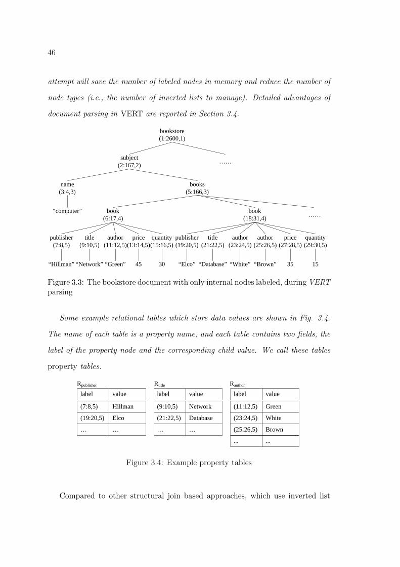
46

attempt will save the number of labeled nodes in memory and reduce the number of

node types (i.e., the number of inverted lists to manage). Detailed advantages of

document parsing in VERT are reported in Section 3.4.

bookstore(1:5000,1)

subject(2:307,2)

name(3:6,3)


book(8:29,4)

title(13:16,5)

author(17:20,5)

publisher(9:12,5)

price(21:24,5)

quantity(25:28,5)

“Hillman”(10:11,6)

“Network”(14:15,6)

“Green”(18:19,6)

45(22:23,6)

30(26:27,6)

……

……

subject

name book

title

“Network”

books(7:306,3)

book(30:55,4)

title(35:38,5)

author(39:42,5)

publisher(31:34,5)

price(47:50,5)

quantity(51:54,5)

“Elco”(32:33,6)


“White”(40:41,6)

35(48:49,6)

15(52:53,6)

author(43:46,5)

“Brown”(44:45,6)

book

title

“Network”

author

book

title

join

(a) (b)

Content Search



ExtractionStep 3



bookstore(1:2600,1)

subject(2:167,2)

name(3:4,3)

“computer” book(6:17,4)

title(9:10,5)

author(11:12,5)

publisher(7:8,5)

price(13:14,5)

quantity(15:16,5)

“Hillman” “Network” “Green” 45 30

……

……

books(5:166,3)

book(18:31,4)

title(21:22,5)

author(23:24,5)

publisher(19:20,5)

price(27:28,5)

quantity(29:30,5)


author(25:26,5)

“Brown”

Figure 3.3: The bookstore document with only internal nodes labeled, during VERTparsing

Some example relational tables which store data values are shown in Fig. 3.4.

The name of each table is a property name, and each table contains two fields, the

label of the property node and the corresponding child value. We call these tables

property tables.

bookstore(1:5000,1)

subject(2:307,2)

name(3:6,3)


book(8:29,4)

title(13:16,5)

author(17:20,5)

publisher(9:12,5)

price(21:24,5)

quantity(25:28,5)

“Hillman”(10:11,6)

“Network”(14:15,6)

“Green”(18:19,6)

45(22:23,6)

30(26:27,6)

……

……

subject

name book

title

“Network”

books(7:306,3)

book(30:55,4)

title(35:38,5)

author(39:42,5)

publisher(31:34,5)

price(47:50,5)

quantity(51:54,5)

“Elco”(32:33,6)


“White”(40:41,6)

35(48:49,6)

15(52:53,6)

author(43:46,5)

“Brown”(44:45,6)

book

title

“Network”

author

book

title

join

(a) (b)

Content Search



ExtractionStep 3



bookstore(1:2600,1)

subject(2:167,2)

name(3:4,3)


title(9:10,5)

author(11:12,5)

publisher(7:8,5)

price(13:14,5)

quantity(15:16,5)


……

……

books(5:166,3)

book(18:31,4)

title(21:22,5)

author(23:24,5)

publisher(19:20,5)

price(27:28,5)

quantity(29:30,5)


author(25:26,5)

“Brown”

label value

(7:8,5) Hillman

Rpublisher

(19:20,5) Elco

… …

value

Network

Rtitle

Database

…

...

value

Green

Rauthor

White

Brown

label

(9:10,5)

(21:22,5)

…

...

label

(11:12,5)

(23:24,5)

(25:26,5)

label value

(2:15,2) XML

Rbook/title

(16:27,2) Databases

... ...

value

Stein

Rbook/author

Dellwig

Paredaens

...

value

32

Rbook/price

17

...

label

(2:15,2)

(2:15,2)

(16:27,2)

...

label

(2:15,2)

(16:27,2)

...

Figure 3.4: Example property tables

Compared to other structural join based approaches, which use inverted list

47

to index values, our approach to use relational tables for values has the following

advantages:

• Relational tables can support advanced search, such as numeric range search

and containment search for values. These advanced search is highly expected

by users in XPath expressions. Other approach cannot perform advanced

search easily when they employ inverted lists to index both structural nodes

and value nodes.

• Using relational table, we can both select the property labels based on a

given value and selection child value based on a given property table. This

feature is very important because when we perform content search we need to

extract labels based on values for further structural join, whereas to answer

the query we need to extract values based on property labels. However, in

other approaches, inverted list can only be used to get a list of labels for

structural join. To answer the query, they have to access the document again

to fetch the values based on property labels. This violates the purpose of

using inverted lists to save I/O cost in these approaches.

Similar to inverted list, relational table also plays an index role to aid twig

pattern query processing, which is presented in the next section. As a result, how

to cope with document updates is an important issue for both inverted lists and

relational tables. Inverted list is widely used to process different forms of queries

for years, e.g., twig pattern query and keyword query. There are different ways

to maintain an inverted list for updates, e.g., employing a B-tree for each list.

Here we focus on the maintenance of relational tables when the XML document

is updated. Actually relational tables are easy to maintain. If the document is

dynamic, which means there are frequent updates to the document, we can adopt

48

a dynamic labeling scheme to label the document so that the update will not cause

re-labeling for remaining document nodes. Thus, when some document nodes are

deleted, we simply delete the corresponding tuples in the relational tables; while

when some new nodes are added, we assign them new labels, and put them into

corresponding relational tables without affecting the existence of other tuples.

3.2.4 Query processing in VERT

As shown in Fig. 3.2, query processing in VERT contains three steps: content

search and query rewriting, structural search, and value extraction. Theoretically,

the first two steps, i.e., content search and structural search, can be reordered.

The reason that we perform content search before structural search is that content

search normally results high selectivity. By performing content search first, we can

significantly reduce the inverted list size of relevant query nodes. This is similar

to selection push-ahead in relational query optimizers. The pseudo-code of VERT

query processing is presented in Algorithm 3.2.

We first perform content search in Line 2-8. The algorithm recursively han-

dles all value comparisons in two phases: creating new inverted lists based on the

predicates and rewriting the query to remove the processed value comparisons. In

more details, Line 3-6 execute SQL selection in the corresponding property tables

based on the value comparison, and then put all the selected labels, which satisfy

the value comparison, into the new inverted lists for the corresponding property

node. Line 7 rewrites the query in such a way that every value comparison and

its parent property are replaced by a new query node which has an identical name

as the corresponding new inverted list. The second step is using TwigStack or

other efficient structural join algorithms to process the simplified query with new

inverted lists in Line 10-11. Last in line 13, we can extract actual values based on

49

Algorithm 3.2 VERT query processing

Input: A query Q and necessary inverted lists and relational tablesOutput: A set of value results answering Q

1: //step 1: perform content search, construct new inverted lists and rewrite thequery

2: while there are more value comparisons in predicates of Q do3: let c be the next value comparison, and p be its property (parent element or

attribute)4: create a new inverted list Tp′ for p5: select the labels based on c from the table Rp

6: put the selected labels into Tp′7: rewrite the query to replace the sub-structure p/c by p′

8: end while9: //step 2: perform structural search on the rewritten query with new inverted

lists10: process the rewritten pattern of Q using any existing efficient structural join

algorithm like TwigStack, to get labels for output nodes11: delete newly created inverted lists12: //step 3: extract query answer13: extract and refine actual values with labels from corresponding tables, if the

output node is a property node; otherwise access the document to return sub-trees

node labels from the corresponding table, if the output node is a property node.

When different node labels contribute to the same value answer, we can refine the

result by removing the duplicates.

Example 3.2. Now we use the twig pattern query in Fig. 1.3(a) to illustrate

how VERT works. In the first step, VERT identifies the only predicate with value

comparison is title=“Network”. During content search, VERT executes an SQL

selection in the table Rtitle to get all the labels of element title which have a value

of “Network”. Then we put the selected labels into the new inverted list for title,

Ttitle′. After that we rewrite the twig pattern query to replace the sub-structure of

the node title and its child node “Network” by title’. The rewritten query is shown

in Fig. 3.5(a). Now the query node title’ corresponds to the newly created inverted

list Ttitle′, in which all the labels satisfy the constraint title=“Network”. To clearly

50

explain title’ in the rewritten query, we use titleNetwork in Fig. 3.5(a). Finally

we use a twig pattern matching algorithm, e.g., TwigStack to process the rewritten

query in Fig. 3.5(a), with the inverted list Ttitle′ for the node titleNetwork.

bookstore(1:5000,1)

subject(2:307,2)

name(3:6,3)


book(8:29,4)

title(13:16,5)

author(17:20,5)

publisher(9:12,5)

price(21:24,5)

quantity(25:28,5)

“Hillman”(10:11,6)

“Network”(14:15,6)

“Green”(18:19,6)

45(22:23,6)

30(26:27,6)

……

……

subject

name book

title

“Network”

books(7:306,3)

book(30:55,4)

title(35:38,5)

author(39:42,5)

publisher(31:34,5)

price(47:50,5)

quantity(51:54,5)

“Elco”(32:33,6)


“White”(40:41,6)

35(48:49,6)

15(52:53,6)

author(43:46,5)

“Brown”(44:45,6)

book

title

“Network”

author

book

title

join

(a) (b)

Content Search



ExtractionStep 3



bookstore(1:2600,1)

subject(2:167,2)

name(3:4,3)


title(9:10,5)

author(11:12,5)

publisher(7:8,5)

price(13:14,5)

quantity(15:16,5)


……

……

books(5:166,3)

book(18:31,4)

title(21:22,5)

author(23:24,5)

publisher(19:20,5)

price(27:28,5)

quantity(29:30,5)


author(25:26,5)

“Brown”

label value

(7:8,5) Hillman

Rpublisher

(19:20,5) Elco

… …

value

Network

Rtitle

Database

…

...

value

Green

Rauthor

White

Brown

label

(9:10,5)

(21:22,5)

…

...

label

(11:12,5)

(23:24,5)

(25:26,5)

label value

(2:15,2) XML

Rbook/title

(16:27,2) Databases

... ...

value

Stein

Rbook/author

Dellwig

Paredaens

...

value

32

Rbook/price

17

...

label

(2:15,2)

(2:15,2)

(16:27,2)

...

label

(2:15,2)

(16:27,2)

...

subject

name book

titleNetwork

subject

booktitle=“Network”name

(a) Rewritten query example

bookstore(1:5000,1)

subject(2:307,2)

name(3:6,3)


book(8:29,4)

title(13:16,5)

author(17:20,5)

publisher(9:12,5)

price(21:24,5)

quantity(25:28,5)

“Hillman”(10:11,6)

“Network”(14:15,6)

“Green”(18:19,6)

45(22:23,6)

30(26:27,6)

……

……

subject

name book

title

“Network”

books(7:306,3)

book(30:55,4)

title(35:38,5)

author(39:42,5)

publisher(31:34,5)

price(47:50,5)

quantity(51:54,5)

“Elco”(32:33,6)


“White”(40:41,6)

35(48:49,6)

15(52:53,6)

author(43:46,5)

“Brown”(44:45,6)

book

title

“Network”

author

book

title

(t1) (t2)

Content Search



ExtractionStep 3



bookstore(1:2600,1)

subject(2:167,2)

name(3:4,3)


title(9:10,5)

author(11:12,5)

publisher(7:8,5)

price(13:14,5)

quantity(15:16,5)


……

……

books(5:166,3)

book(18:31,4)

title(21:22,5)

author(23:24,5)

publisher(19:20,5)

price(27:28,5)

quantity(29:30,5)


author(25:26,5)

“Brown”

label value

(7:8,5) Hillman

Rpublisher

(19:20,5) Elco

… …

value

Network

Rtitle

Database

…

...

value

Green

Rauthor

White

Brown

label

(9:10,5)

(21:22,5)

…

...

label

(11:12,5)

(23:24,5)

(25:26,5)

label value

(6:17,4) Hillman

Rbook/publisher

(18:31,4) Elco

… …

value

Network

Rbook/title

Database

…

…

value

Green

Rbook/author

White

Brown

label

(6:17,4)

(18:31,4)

…

…

label

(6:17,4)

(18:31,4)

(18:31,4)

subject

name book

titleNetwork

subject


author

subject

name book

title

“Network”

price

>40

subject

booktitle=“Network”&price>40name

label publisher

(6:17,4) Hillman

Rbook

(18:31,4) Elco

… …

title

Network

Database

…

price

45

35

…

quantity

30

15

…

…

value

Green

Rbook/author

White

Brown

…

label

(6:17,4)

(18:31,4)

(18:31,4)

object property

book second_title

Rrare_property

magazine sale_region

book second_title

label

(76:89,4)

(128:143,4)

(282:299,4)

value

An introduction to data mining

Singapore

A first course

… … … …

bookstore(1:2800,1)

subject(2:197,2)

name(3:4,3)

“computer”

book(9:20,5)

title(12:13,6)

author(14:15,6)

publisher(10:11,6)

price(16:17,6)

quantity(18:19,6)


……

……

branches(5:196,3)

book(21:34,5)

title(24:25,6)

author(26:27,6)

publisher(22:23,6)

price(30:31,6)

quantity(32:33,6)


author(28:29,6)

“Brown”

branch(6:107,4)

code(7:8,5)

“001”

……

subject

name branch

book

quantity

“ computer” code

<20

subjectname=“computer”

branch

bookquantity<20code

labelbranch labelbook

(6:107,4) (9:20,5)

Rbranch-book

(6:107,4) (21:34,5)

… …

quantity

30

15

…


branchbranch-book.quantity<20

code

Joining t1 and t2 based on author value

subject

name book

>20

subject

name book

<20

(b) Invalid query example

Figure 3.5: A rewritten query example and an invalid twig pattern query example

As described in Section 1.2.1, twig pattern query is an intermediate query rep-

resentation for some formal XML query languages, e.g., XPath and XQuery. Since

in the predicate of an XPath or XQuery query, a value must link to a property

through an operator, e.g., price<20, the value comparison in the corresponding

twig pattern representation must be a child (‘/’), instead of a descendant (“//”) of

an internal query node. A twig pattern expression shown in Fig. 3.5(b) is invalid,

as the value comparison follows a “//” edge. Semantically, this query cannot be

well interpreted; and practically, this query will never appear in XPath or XQuery

expressions. We do not consider such invalid twig patterns, thus our algorithm can

perform any content search using property tables.

Note that VERT saves I/O cost in value extraction when the output node is

a property node, because we do not need to visit the original document, but only

access relevant relational tables to find values. However, if the output node matches

some internal nodes with subelements in the document, the result should be the

whole subtree rooted at each matched node, instead of a single value. In this case,

VERT has no advantage in result return over other approaches.

51

3.2.5 Analysis of VERT

In this section, we analyze our algorithm in five points of view: the management of

labeled nodes and inverted lists, content search for predicates and value extraction

for final results, the size of inverted lists to be searched, the number of structural

joins required during query processing, and the support for advanced search.

Label and inverted list management. Normally in a large XML document,

value nodes take a high proportion to all document nodes. VERT combines

values to their parent elements, and avoids labeling value nodes separately.

Then the number of labeled nodes in memory will be greatly reduced. More-

over, VERT also has advantage in inverted list management. Since the high

variety of values is ignored during inverted list construction in VERT, the

number of inverted lists is limited to the number of element or attribute

types. In this point of view, the problem of managing tremendous number of

inverted lists in previous work can be solved.

Content search and value extraction. Consider the previous example that a

query aims to find the books with price of 35 and output their titles. As men-

tioned earlier, when we perform content search for this query using existing

approaches we have to read the inverted list for ‘35’, which contains labels

with different semantics like the price of a book and the quantity of a book.

To mix them together will cause unnecessary search. Instead of searching in

inverted lists, VERT handles content search in semantic tables. In this case,

we just move into the property table for price and avoid searching for the

value ‘35’ under quantity. Furthermore, after getting all the satisfied occur-

rences of the output node title in terms of labels, we aim to find the actual

value under each title. Previous approaches have to refer to the document

52

again to fetch values because the inverted lists cannot help to extract values

based on parent node labels. VERT can efficiently get the desired values

without considering the document storage because all the values are stored

in tables and we can directly extract them using the labels of their associated

property by SQL selections. Also, if different node labels contribute to the

same value answer, we can refine the returned answer by removing duplicates.

In a word, relational tables are not only helpful for content search, but also

usable to extract desired values.

Inverted list searching reduction. Performing content search before structural

join in VERT can significantly reduce the size of relevant inverted lists. Con-

sider the query in Fig. 1.3(a). Assume there is only one book called “Net-

work”. If the number of different books is b, the size of the inverted list for

the element title is also b in previous approaches. Then we need O(b) to

scan all the labels in the inverted list for title. VERT processes selection in

advance, so that the new inverted list for title is created based on the value

“Network”. In this case the new inverted list has only 1 label inside based on

our assumption. Normally, when the selectivity of an element is high, like in

this example, VERT can be very efficient in structural search because it sig-

nificantly reduces the searching in inverted lists for the relevant nodes. This

is similar to the selection push-ahead in SQL query processing in relational

databases.

Query nodes and structural joins reduction. There are two factors driving a

high performance of structural search in VERT. One is inverted list searching

reduction as mentioned above and the other factor is query nodes and struc-

tural joins reduction in the rewritten query. Still consider the original and

rewritten query in Fig. 1.3(a) and 2.1. The rewritten query has only three

53

edges which need structural joins, while the original query has four. Also

when we rewrite the query, we remove the query nodes of value comparison.

This naturally simplifies the query. Optimizations to further reduce the size

of inverted lists and the number of both query nodes and structural joins will

be discussed in the next section.

Advanced search support. Advanced search is quite common in real life queries.

For example, in an XPath expression, numeric range search and the contains

function are usually issued in predicates. Since VERT can use any exist-

ing RDBMS to manage property tables, all the advanced search which are

supported by the relational system are also supported in VERT. Also VERT

permits conjunction or disjunction of value comparisons appearing as a leaf

node in a twig pattern query.

We can observe that sequential scans and structural joins for labels of both

property node and value node in previous work are replaced by selections in se-

mantic tables in VERT. Actually in any relational database system, such table

selection can be done very efficiently. It is not surprising that replacing structural

join by selection for content search will improve the overall performance.

Generally, VERT gains benefit from performing content search ahead of struc-

tural search, and then reduce the complexity of structural search. Thus most

advantages discussed in this section hold only for queries with value predicates,

which are commonly seen in real life. When a query does not have value compar-

ison as predicate, the first part in our algorithm, i.e., the content search part will

be ignored. Then we just follow any existing structural join algorithm to perform

structural search directly. In this case, our algorithm is the same as other existing

algorithms.

54

3.3 Semantic optimizations

Tables in VERT are built based on the semantic relationship between property and

value. That is why we call them property tables. Using property tables to perform

content search may still not efficient enough in some cases. We notice that object

is an important information unit for most queries. In this section, we optimize

the property tables to be object based, to further improve the query processing

efficiency.

3.3.1 Optimization 1: object/property table

Motivation:

We identify two efficiency problems with property table to process twig pattern

queries. The first problem is that the property table may produce redundant labels

during content search. Consider a query to find the title of all books with price

less than 35. To process this query, we need to find all price labels in the price

table with value less than 35. However, if the bookstore document also contains

magazine or other products with the property price, many of the selected labels

may stand for price of other products and it is redundant to use them to construct

the new inverted list for book price. The second problem is the redundant search

on other relevant inverted lists. Generally, by specifying conditions on certain

properties, most queries aim to find the associated object and then get some other

property values of that object. Consider the query in Fig. 1.3(a). Suppose there

are b books in the bookstore and only one of them is called “Network”. After

VERT rewrites the query in Fig. 3.5(a), the size of the inverted list for title is

reduced to 1. However the size of the inverted list for book is still b, which means

we need to search all the b labels though we know only one of them matches the

55

label in the title inverted list. To solve these two efficiency problems, we propose

an optimization scheme based on the relationship between object and property.

Optimization:

Instead of storing each value with the label of its associated property node, we can

put the property value and the label of the corresponding object node into relational

tables. For example, in the bookstore document we put values for publisher, title

and so forth with labels of the corresponding object book into object/property tables

as shown in Fig. 3.6(a). The ‘label’ field of each table stores the label of the object

and the following ‘value’ corresponds the value of different properties in different

tables. When we perform a content search, we can directly select the object labels

in the corresponding object/property tables and construct a new inverted list for

the object. Then to process the query in Fig. 1.3(a), we perform the content

search using Rbook/title to restrict the book labels based on the condition on title

value. After that the query can be further rewritten accordingly, as shown in

Fig. 3.6(b), where Tbook′ is the new inverted list for the element book and we use

booktitle=“Network” is to explicitly explain book’. Now we not only reduce the size

of Tbook, but also further reduce the number of structural joins and the number of

query nodes by one. Then we can get a higher performance when we execute the

simplified query.

Discussion:

Ordinal Column: This optimization may lose order information for multi-valued

properties. Such information may be important in some cases. For example, the

order of authors is important, but from the book/author table we cannot tell which

author comes first for a certain book. To solve this limitation, we can simply add

56

bookstore(1:5000,1)

subject(2:307,2)

name(3:6,3)


book(8:29,4)

title(13:16,5)

author(17:20,5)

publisher(9:12,5)

price(21:24,5)

quantity(25:28,5)

“Hillman”(10:11,6)

“Network”(14:15,6)

“Green”(18:19,6)

45(22:23,6)

30(26:27,6)

……

……

subject

name book

title

“Network”

books(7:306,3)

book(30:55,4)

title(35:38,5)

author(39:42,5)

publisher(31:34,5)

price(47:50,5)

quantity(51:54,5)

“Elco”(32:33,6)


“White”(40:41,6)

35(48:49,6)

15(52:53,6)

author(43:46,5)

“Brown”(44:45,6)

book

title

“Network”

author

book

title

join:

(a) (b)

Content Search



ExtractionStep 3



bookstore(1:2600,1)

subject(2:167,2)

name(3:4,3)


title(9:10,5)

author(11:12,5)

publisher(7:8,5)

price(13:14,5)

quantity(15:16,5)


……

……

books(5:166,3)

book(18:31,4)

title(21:22,5)

author(23:24,5)

publisher(19:20,5)

price(27:28,5)

quantity(29:30,5)


author(25:26,5)

“Brown”

label value

(7:8,5) Hillman

Rpublisher

(19:20,5) Elco

… …

value

Network

Rtitle

Database

…

...

value

Green

Rauthor

White

Brown

label

(9:10,5)

(21:22,5)

…

...

label

(11:12,5)

(23:24,5)

(25:26,5)

label value

(6:17,4) Hillman

Rbook/publisher

(18:31,4) Elco

… …

value

Network

Rbook/title

Database

…

…

value

Green

Rbook/author

White

Brown

label

(6:17,4)

(18:31,4)

…

…

label

(6:17,4)

(18:31,4)

(18:31,4)

subject

name book

titleNetwork

subject


author

(a) Tables in VERT Optimization 1

bookstore(1:5000,1)

subject(2:307,2)

name(3:6,3)


book(8:29,4)

title(13:16,5)

author(17:20,5)

publisher(9:12,5)

price(21:24,5)

quantity(25:28,5)

“Hillman”(10:11,6)

“Network”(14:15,6)

“Green”(18:19,6)

45(22:23,6)

30(26:27,6)

……

……

subject

name book

title

“Network”

books(7:306,3)

book(30:55,4)

title(35:38,5)

author(39:42,5)

publisher(31:34,5)

price(47:50,5)

quantity(51:54,5)

“Elco”(32:33,6)


“White”(40:41,6)

35(48:49,6)

15(52:53,6)

author(43:46,5)

“Brown”(44:45,6)

book

title

“Network”

author

book

title

join

(a) (b)

Content Search



ExtractionStep 3



bookstore(1:2600,1)

subject(2:167,2)

name(3:4,3)


title(9:10,5)

author(11:12,5)

publisher(7:8,5)

price(13:14,5)

quantity(15:16,5)


……

……

books(5:166,3)

book(18:31,4)

title(21:22,5)

author(23:24,5)

publisher(19:20,5)

price(27:28,5)

quantity(29:30,5)


author(25:26,5)

“Brown”

label value

(7:8,5) Hillman

Rpublisher

(19:20,5) Elco

… …

value

Network

Rtitle

Database

…

...

value

Green

Rauthor

White

Brown

label

(9:10,5)

(21:22,5)

…

...

label

(11:12,5)

(23:24,5)

(25:26,5)

label value

(2:15,2) XML

Rbook/title

(16:27,2) Databases

... ...

value

Stein

Rbook/author

Dellwig

Paredaens

...

value

32

Rbook/price

17

...

label

(2:15,2)

(2:15,2)

(16:27,2)

...

label

(2:15,2)

(16:27,2)

...

subject

name book

titleNetwork

subject


(b) Rewritten queryfor Fig 1.3(a) withinverted list size ofbooktitle=“Network”=|Tbook′ |=1

Figure 3.6: Tables and rewritten query under VERT Optimization 1

an additional column in the object/property tables for multi-valued properties, to

indicate the ordinal information.

3.3.2 Optimization 2: object table

Motivation:

It is quite normal that some queries contain multiple predicates on a common

object. Consider the query shown in Fig. 3.7(a), which aims to find the subject

of the book with title of “Network” and price less than 40. To answer this query,

Optimization 1 needs to find the labels of books with title of “Network” and labels

of books with price less than 40 separately using the object/property tables, and

intersect the two sets of labels. With semantic information, we know that title and

price are both properties of the object book. If we have one table for this object

that contains the both properties, books satisfying these two constraints can be

found directly with one SQL selection, and then the intermediate results can be

avoided.

57

bookstore(1:5000,1)

subject(2:307,2)

name(3:6,3)


book(8:29,4)

title(13:16,5)

author(17:20,5)

publisher(9:12,5)

price(21:24,5)

quantity(25:28,5)

“Hillman”(10:11,6)

“Network”(14:15,6)

“Green”(18:19,6)

45(22:23,6)

30(26:27,6)

……

……

subject

name book

title

“Network”

books(7:306,3)

book(30:55,4)

title(35:38,5)

author(39:42,5)

publisher(31:34,5)

price(47:50,5)

quantity(51:54,5)

“Elco”(32:33,6)


“White”(40:41,6)

35(48:49,6)

15(52:53,6)

author(43:46,5)

“Brown”(44:45,6)

book

title

“Network”

author

book

title

join:

(a) (b)

Content Search



ExtractionStep 3



bookstore(1:2600,1)

subject(2:167,2)

name(3:4,3)


title(9:10,5)

author(11:12,5)

publisher(7:8,5)

price(13:14,5)

quantity(15:16,5)


……

……

books(5:166,3)

book(18:31,4)

title(21:22,5)

author(23:24,5)

publisher(19:20,5)

price(27:28,5)

quantity(29:30,5)


author(25:26,5)

“Brown”

label value

(7:8,5) Hillman

Rpublisher

(19:20,5) Elco

… …

value

Network

Rtitle

Database

…

...

value

Green

Rauthor

White

Brown

label

(9:10,5)

(21:22,5)

…

...

label

(11:12,5)

(23:24,5)

(25:26,5)

label value

(6:17,4) Hillman

Rbook/publisher

(18:31,4) Elco

… …

value

Network

Rbook/title

Database

…

…

value

Green

Rbook/author

White

Brown

label

(6:17,4)

(18:31,4)

…

…

label

(6:17,4)

(18:31,4)

(18:31,4)

subject

name book

titleNetwork

subject


author

subject

name book

title

“Network”

price

<40

(a) Query with multiple value predicates underthe same object

bookstore(1:5000,1)

subject(2:307,2)

name(3:6,3)


book(8:29,4)

title(13:16,5)

author(17:20,5)

publisher(9:12,5)

price(21:24,5)

quantity(25:28,5)

“Hillman”(10:11,6)

“Network”(14:15,6)

“Green”(18:19,6)

45(22:23,6)

30(26:27,6)

……

……

subject

name book

title

“Network”

books(7:306,3)

book(30:55,4)

title(35:38,5)

author(39:42,5)

publisher(31:34,5)

price(47:50,5)

quantity(51:54,5)

“Elco”(32:33,6)


“White”(40:41,6)

35(48:49,6)

15(52:53,6)

author(43:46,5)

“Brown”(44:45,6)

book

title

“Network”

author

book

title

join:

(a) (b)

Content Search



ExtractionStep 3



bookstore(1:2600,1)

subject(2:167,2)

name(3:4,3)


title(9:10,5)

author(11:12,5)

publisher(7:8,5)

price(13:14,5)

quantity(15:16,5)


……

……

books(5:166,3)

book(18:31,4)

title(21:22,5)

author(23:24,5)

publisher(19:20,5)

price(27:28,5)

quantity(29:30,5)


author(25:26,5)

“Brown”

label value

(7:8,5) Hillman

Rpublisher

(19:20,5) Elco

… …

value

Network

Rtitle

Database

…

...

value

Green

Rauthor

White

Brown

label

(9:10,5)

(21:22,5)

…

...

label

(11:12,5)

(23:24,5)

(25:26,5)

label value

(6:17,4) Hillman

Rbook/publisher

(18:31,4) Elco

… …

value

Network

Rbook/title

Database

…

…

value

Green

Rbook/author

White

Brown

label

(6:17,4)

(18:31,4)

…

…

label

(6:17,4)

(18:31,4)

(18:31,4)

subject

name book

titleNetwork

subject


author

subject

name book

title

“Network”

price

>40

subject

booktitle=“Network”&price<40name

(b) Rewritten query for Fig 3.7(a) underOptimization 2

Figure 3.7: Example query with multiple value predicates under the same objectand its rewritten query in Optimization 2

Optimization:

A simple idea is to merge the object/property tables in Optimization 1 based on

the same objects. For multi-valued properties, such as author in our example,

it is not practical to merge it with other properties. In this case, we can merge

all the single-valued properties of an object into one object table and keep the

object/property tables for multi-valued properties. The resulting tables for the

object book in the bookstore document under this optimization are shown in Fig.

3.8. In Rbook, each label of book is stored with all the single-valued property values

of that book. When we process queries with multiple predicates on single-valued

properties of an object, we can do selection in that object table based on multiple

constraints in one time. For example, to process the query in Fig. 3.7(a), we can

select book labels based on the two predicates in Rbook with one SQL selection.

Then the original query can be rewritten as shown in Fig. 3.7(b). Comparing with

the Optimization 1 approach, we further simplify the query and prune intermediate

results for the two predicates.

58

bookstore(1:5000,1)

subject(2:307,2)

name(3:6,3)


book(8:29,4)

title(13:16,5)

author(17:20,5)

publisher(9:12,5)

price(21:24,5)

quantity(25:28,5)

“Hillman”(10:11,6)

“Network”(14:15,6)

“Green”(18:19,6)

45(22:23,6)

30(26:27,6)

……

……

subject

name book

title

“Network”

books(7:306,3)

book(30:55,4)

title(35:38,5)

author(39:42,5)

publisher(31:34,5)

price(47:50,5)

quantity(51:54,5)

“Elco”(32:33,6)


“White”(40:41,6)

35(48:49,6)

15(52:53,6)

author(43:46,5)

“Brown”(44:45,6)

book

title

“Network”

author

book

title

join:

(a) (b)

Content Search



ExtractionStep 3



bookstore(1:2600,1)

subject(2:167,2)

name(3:4,3)


title(9:10,5)

author(11:12,5)

publisher(7:8,5)

price(13:14,5)

quantity(15:16,5)


……

……

books(5:166,3)

book(18:31,4)

title(21:22,5)

author(23:24,5)

publisher(19:20,5)

price(27:28,5)

quantity(29:30,5)


author(25:26,5)

“Brown”

label value

(7:8,5) Hillman

Rpublisher

(19:20,5) Elco

… …

value

Network

Rtitle

Database

…

...

value

Green

Rauthor

White

Brown

label

(9:10,5)

(21:22,5)

…

...

label

(11:12,5)

(23:24,5)

(25:26,5)

label value

(6:17,4) Hillman

Rbook/publisher

(18:31,4) Elco

… …

value

Network

Rbook/title

Database

…

…

value

Green

Rbook/author

White

Brown

label

(6:17,4)

(18:31,4)

…

…

label

(6:17,4)

(18:31,4)

(18:31,4)

subject

name book

titleNetwork

subject


author

subject

name book

title

“Network”

price

>40

subject


label publisher

(6:17,4) Hillman

Rbook

(18:31,4) Elco

… …

title

Network

Database

…

price

45

35

…

quantity

30

15

…

…

value

Green

Rbook/author

White

Brown

…

label

(6:17,4)

(18:31,4)

(18:31,4)

Figure 3.8: Tables for book in the bookstore document under VERT Optimization2

Discussion:

Mixed table selection: If the multiple predicates involve both single-valued

properties and multi-valued properties, we can perform selection for all single-

valued properties in the object table, and then intersect the result with the selection

result from the object/property tables for the multi-valued properties.

Rare property: Properties may optionally appear under the associated objects.

In some cases, the occurrence of certain properties may be rare. We call such

properties rare properties. Suppose in the bookstore document, only a few books

have a second title, then second title is a rare property. If we put this rare property

as a column in the book table, there will be too many NULL entries.

bookstore(1:5000,1)

subject(2:307,2)

name(3:6,3)


book(8:29,4)

title(13:16,5)

author(17:20,5)

publisher(9:12,5)

price(21:24,5)

quantity(25:28,5)

“Hillman”(10:11,6)

“Network”(14:15,6)

“Green”(18:19,6)

45(22:23,6)

30(26:27,6)

……

……

subject

name book

title

“Network”

books(7:306,3)

book(30:55,4)

title(35:38,5)

author(39:42,5)

publisher(31:34,5)

price(47:50,5)

quantity(51:54,5)

“Elco”(32:33,6)


“White”(40:41,6)

35(48:49,6)

15(52:53,6)

author(43:46,5)

“Brown”(44:45,6)

book

title

“Network”

author

book

title

join:

(a) (b)

Content Search



ExtractionStep 3



bookstore(1:2600,1)

subject(2:167,2)

name(3:4,3)


title(9:10,5)

author(11:12,5)

publisher(7:8,5)

price(13:14,5)

quantity(15:16,5)


……

……

books(5:166,3)

book(18:31,4)

title(21:22,5)

author(23:24,5)

publisher(19:20,5)

price(27:28,5)

quantity(29:30,5)


author(25:26,5)

“Brown”

label value

(7:8,5) Hillman

Rpublisher

(19:20,5) Elco

… …

value

Network

Rtitle

Database

…

...

value

Green

Rauthor

White

Brown

label

(9:10,5)

(21:22,5)

…

...

label

(11:12,5)

(23:24,5)

(25:26,5)

label value

(6:17,4) Hillman

Rbook/publisher

(18:31,4) Elco

… …

value

Network

Rbook/title

Database

…

…

value

Green

Rbook/author

White

Brown

label

(6:17,4)

(18:31,4)

…

…

label

(6:17,4)

(18:31,4)

(18:31,4)

subject

name book

titleNetwork

subject


author

subject

name book

title

“Network”

price

>40

subject


label publisher

(6:17,4) Hillman

Rbook

(18:31,4) Elco

… …

title

Network

Database

…

price

45

35

…

quantity

30

15

…

…

value

Green

Rbook/author

White

Brown

…

label

(6:17,4)

(18:31,4)

(18:31,4)

object property

book second_title

Rrare_property


book second_title

label

(76:89,4)

(128:143,4)

(282:299,4)

value


Singapore

A first course

… … … …

Figure 3.9: Table for rare properties

Some relational database systems can deal with the case of sparse attribute in

59

the physical storage. In case some other systems do not have this function, we can

maintain a rare property table to store all such rare properties. The rare property

table contains: the object name, the rare property name, the object label and the

property value. Suppose in the bookstore document, second title is a rare property

of book and sale region is a rare property of magazine, the rare property table for

this document is shown in Fig. 3.9. Queries involving rare properties are processed

by accessing the rare property table with the object name and the property name.

Vertical partitioning: Object table is obtained by merging the object/property

tables for all the single-valued property under the same object. When there are

many single-valued properties under a certain object, the tuple size of the corre-

sponding object table will be too large. When we perform a selection based on only

a few properties, all other properties are also loaded. This results a high I/O cost.

A common way in RDBMS design to reduce such I/O cost is the vertical parti-

tioning of a table ([95]). We can refer to the query history to see which properties

often appear together in the same query, and then split the original object table

into several partitions according to such information. Since vertical partitioning is

not a new technique, we do not discuss it any more.

3.3.3 Optimization 3: relationship table

Motivation:

Unlike the ER model for relational data, the hierarchical structure of an XML

document cannot reflect the relationships between objects explicitly. However, such

relationships do exist usually. Consider another design of the bookstore document

as shown in Fig. 3.10, in which the books under each subject are also grouped by

different branches.

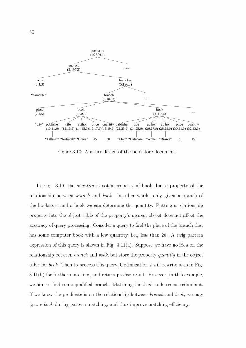
60

bookstore(1:5000,1)

subject(2:307,2)

name(3:6,3)


book(8:29,4)

title(13:16,5)

author(17:20,5)

publisher(9:12,5)

price(21:24,5)

quantity(25:28,5)

“Hillman”(10:11,6)

“Network”(14:15,6)

“Green”(18:19,6)

45(22:23,6)

30(26:27,6)

……

……

subject

name book

title

“Network”

books(7:306,3)

book(30:55,4)

title(35:38,5)

author(39:42,5)

publisher(31:34,5)

price(47:50,5)

quantity(51:54,5)

“Elco”(32:33,6)


“White”(40:41,6)

35(48:49,6)

15(52:53,6)

author(43:46,5)

“Brown”(44:45,6)

book

title

“Network”

author

book

title

(t1) (t2)

Content Search



ExtractionStep 3



bookstore(1:2600,1)

subject(2:167,2)

name(3:4,3)


title(9:10,5)

author(11:12,5)

publisher(7:8,5)

price(13:14,5)

quantity(15:16,5)


……

……

books(5:166,3)

book(18:31,4)

title(21:22,5)

author(23:24,5)

publisher(19:20,5)

price(27:28,5)

quantity(29:30,5)


author(25:26,5)

“Brown”

label value

(7:8,5) Hillman

Rpublisher

(19:20,5) Elco

… …

value

Network

Rtitle

Database

…

...

value

Green

Rauthor

White

Brown

label

(9:10,5)

(21:22,5)

…

...

label

(11:12,5)

(23:24,5)

(25:26,5)

label value

(6:17,4) Hillman

Rbook/publisher

(18:31,4) Elco

… …

value

Network

Rbook/title

Database

…

…

value

Green

Rbook/author

White

Brown

label

(6:17,4)

(18:31,4)

…

…

label

(6:17,4)

(18:31,4)

(18:31,4)

subject

name book

titleNetwork

subject


author

subject

name book

title

“Network”

price

>40

subject


label publisher

(6:17,4) Hillman

Rbook

(18:31,4) Elco

… …

title

Network

Database

…

price

45

35

…

quantity

30

15

…

…

value

Green

Rbook/author

White

Brown

…

label

(6:17,4)

(18:31,4)

(18:31,4)

object property

book second_title

Rrare_property


book second_title

label

(76:89,4)

(128:143,4)

(282:299,4)

value


Singapore

A first course

… … … …

bookstore(1:2800,1)

subject(2:197,2)

name(3:4,3)

“computer”

book(9:20,5)

title(12:13,6)

author(14:15,6)

publisher(10:11,6)

price(16:17,6)

quantity(18:19,6)


……

……

branches(5:196,3)

book(21:34,5)

title(24:25,6)

author(26:27,6)

publisher(22:23,6)

price(30:31,6)

quantity(32:33,6)


author(28:29,6)

“Brown”

branch(6:107,4)

place(7:8,5)

“city”

……

subject

name branch

book

quantity


<20


branch

bookquantity<20code


(6:107,4) (9:20,5)

Rbranch-book

(6:107,4) (21:34,5)

… …

quantity

30

15

…



code

Joining t1 and t2 based on author value

Figure 3.10: Another design of the bookstore document

In Fig. 3.10, the quantity is not a property of book, but a property of the

relationship between branch and book. In other words, only given a branch of

the bookstore and a book we can determine the quantity. Putting a relationship

property into the object table of the property’s nearest object does not affect the

accuracy of query processing. Consider a query to find the place of the branch that

has some computer book with a low quantity, i.e., less than 20. A twig pattern

expression of this query is shown in Fig. 3.11(a). Suppose we have no idea on the

relationship between branch and book, but store the property quantity in the object

table for book. Then to process this query, Optimization 2 will rewrite it as in Fig.

3.11(b) for further matching, and return precise result. However, in this example,

we aim to find some qualified branch. Matching the book node seems redundant.

If we know the predicate is on the relationship between branch and book, we may

ignore book during pattern matching, and thus improve matching efficiency.

61

bookstore(1:5000,1)

subject(2:307,2)

name(3:6,3)


book(8:29,4)

title(13:16,5)

author(17:20,5)

publisher(9:12,5)

price(21:24,5)

quantity(25:28,5)

“Hillman”(10:11,6)

“Network”(14:15,6)

“Green”(18:19,6)

45(22:23,6)

30(26:27,6)

……

……

subject

name book

title

“Network”

books(7:306,3)

book(30:55,4)

title(35:38,5)

author(39:42,5)

publisher(31:34,5)

price(47:50,5)

quantity(51:54,5)

“Elco”(32:33,6)


“White”(40:41,6)

35(48:49,6)

15(52:53,6)

author(43:46,5)

“Brown”(44:45,6)

book

title

“Network”

author

book

title

join:

(a) (b)

Content Search



ExtractionStep 3



bookstore(1:2600,1)

subject(2:167,2)

name(3:4,3)


title(9:10,5)

author(11:12,5)

publisher(7:8,5)

price(13:14,5)

quantity(15:16,5)


……

……

books(5:166,3)

book(18:31,4)

title(21:22,5)

author(23:24,5)

publisher(19:20,5)

price(27:28,5)

quantity(29:30,5)


author(25:26,5)

“Brown”

label value

(7:8,5) Hillman

Rpublisher

(19:20,5) Elco

… …

value

Network

Rtitle

Database

…

...

value

Green

Rauthor

White

Brown

label

(9:10,5)

(21:22,5)

…

...

label

(11:12,5)

(23:24,5)

(25:26,5)

label value

(6:17,4) Hillman

Rbook/publisher

(18:31,4) Elco

… …

value

Network

Rbook/title

Database

…

…

value

Green

Rbook/author

White

Brown

label

(6:17,4)

(18:31,4)

…

…

label

(6:17,4)

(18:31,4)

(18:31,4)

subject

name book

titleNetwork

subject


author

subject

name book

title

“Network”

price

>40

subject


label publisher

(6:17,4) Hillman

Rbook

(18:31,4) Elco

… …

title

Network

Database

…

price

45

35

…

quantity

30

15

…

…

value

Green

Rbook/author

White

Brown

…

label

(6:17,4)

(18:31,4)

(18:31,4)

object property

book second_title

Rrare_property


book second_title

label

(76:89,4)

(128:143,4)

(282:299,4)

value


Singapore

A first course

… … … …

bookstore(1:2800,1)

subject(2:197,2)

name(3:4,3)

“computer”

book(9:20,5)

title(12:13,6)

author(14:15,6)

publisher(10:11,6)

price(16:17,6)

quantity(18:19,6)


……

……

books(5:196,3)

book(21:34,5)

title(24:25,6)

author(26:27,6)

publisher(22:23,6)

price(30:31,6)

quantity(32:33,6)


author(28:29,6)

“Brown”

branch(6:107,4)

code(7:8,5)

“001”

……

subject

name branch

book

quantity

“ computer” place

<20

subject

name branch

bookquantity<20“ computer” code

(a) Example twig pattern query

bookstore(1:5000,1)

subject(2:307,2)

name(3:6,3)


book(8:29,4)

title(13:16,5)

author(17:20,5)

publisher(9:12,5)

price(21:24,5)

quantity(25:28,5)

“Hillman”(10:11,6)

“Network”(14:15,6)

“Green”(18:19,6)

45(22:23,6)

30(26:27,6)

……

……

subject

name book

title

“Network”

books(7:306,3)

book(30:55,4)

title(35:38,5)

author(39:42,5)

publisher(31:34,5)

price(47:50,5)

quantity(51:54,5)

“Elco”(32:33,6)


“White”(40:41,6)

35(48:49,6)

15(52:53,6)

author(43:46,5)

“Brown”(44:45,6)

book

title

“Network”

author

book

title

(t1) (t2)

Content Search



ExtractionStep 3



bookstore(1:2600,1)

subject(2:167,2)

name(3:4,3)


title(9:10,5)

author(11:12,5)

publisher(7:8,5)

price(13:14,5)

quantity(15:16,5)


……

……

books(5:166,3)

book(18:31,4)

title(21:22,5)

author(23:24,5)

publisher(19:20,5)

price(27:28,5)

quantity(29:30,5)


author(25:26,5)

“Brown”

label value

(7:8,5) Hillman

Rpublisher

(19:20,5) Elco

… …

value

Network

Rtitle

Database

…

...

value

Green

Rauthor

White

Brown

label

(9:10,5)

(21:22,5)

…

...

label

(11:12,5)

(23:24,5)

(25:26,5)

label value

(6:17,4) Hillman

Rbook/publisher

(18:31,4) Elco

… …

value

Network

Rbook/title

Database

…

…

value

Green

Rbook/author

White

Brown

label

(6:17,4)

(18:31,4)

…

…

label

(6:17,4)

(18:31,4)

(18:31,4)

subject

name book

titleNetwork

subject


author

subject

name book

title

“Network”

price

>40

subject


label publisher

(6:17,4) Hillman

Rbook

(18:31,4) Elco

… …

title

Network

Database

…

price

45

35

…

quantity

30

15

…

…

value

Green

Rbook/author

White

Brown

…

label

(6:17,4)

(18:31,4)

(18:31,4)

object property

book second_title

Rrare_property


book second_title

label

(76:89,4)

(128:143,4)

(282:299,4)

value


Singapore

A first course

… … … …

bookstore(1:2800,1)

subject(2:197,2)

name(3:4,3)

“computer”

book(9:20,5)

title(12:13,6)

author(14:15,6)

publisher(10:11,6)

price(16:17,6)

quantity(18:19,6)


……

……

branches(5:196,3)

book(21:34,5)

title(24:25,6)

author(26:27,6)

publisher(22:23,6)

price(30:31,6)

quantity(32:33,6)


author(28:29,6)

“Brown”

branch(6:107,4)

code(7:8,5)

“001”

……

subject

name branch

book

quantity


<20


branch

bookquantity<20place


(6:107,4) (9:20,5)

Rbranch-book

(6:107,4) (21:34,5)

… …

quantity

30

15

…



code

subject

name book

>20

subject

name book

>20

(b) Rewritten query for Fig 3.5(a) under Op-timization 2

Figure 3.11: Example query with predicate on relationship property and its rewrit-ten query in Optimization 2

Optimization:

If we have the semantic information that quantity is actually a property of the

relationship between branch and book, we can include this information in table

construction, i.e., introducing a relationship table. A relationship table stores the

property value and the label of the participating objects of each relationship in-

stance. The example relationship table for the document in Fig. 3.10 is shown in

Fig. 3.12(a). Actually the relationship table is similar to the relationship table in

ER design for structured data. When a relationship involves more than two ob-

jects, the corresponding relationship table will include the labels of all the objects.

Using the knowledge on relationship and the relationship table, the query in Fig.

3.11(a) can be rewritten as in Fig. 3.12(b).

Compared to Optimization 2, the query is further simplified with the semantic

information on relationship. Then the query processing performance will be further

improved.

62

bookstore(1:5000,1)

subject(2:307,2)

name(3:6,3)


book(8:29,4)

title(13:16,5)

author(17:20,5)

publisher(9:12,5)

price(21:24,5)

quantity(25:28,5)

“Hillman”(10:11,6)

“Network”(14:15,6)

“Green”(18:19,6)

45(22:23,6)

30(26:27,6)

……

……

subject

name book

title

“Network”

books(7:306,3)

book(30:55,4)

title(35:38,5)

author(39:42,5)

publisher(31:34,5)

price(47:50,5)

quantity(51:54,5)

“Elco”(32:33,6)


“White”(40:41,6)

35(48:49,6)

15(52:53,6)

author(43:46,5)

“Brown”(44:45,6)

book

title

“Network”

author

book

title

join:

(a) (b)

Content Search



ExtractionStep 3



bookstore(1:2600,1)

subject(2:167,2)

name(3:4,3)


title(9:10,5)

author(11:12,5)

publisher(7:8,5)

price(13:14,5)

quantity(15:16,5)


……

……

books(5:166,3)

book(18:31,4)

title(21:22,5)

author(23:24,5)

publisher(19:20,5)

price(27:28,5)

quantity(29:30,5)


author(25:26,5)

“Brown”

label value

(7:8,5) Hillman

Rpublisher

(19:20,5) Elco

… …

value

Network

Rtitle

Database

…

...

value

Green

Rauthor

White

Brown

label

(9:10,5)

(21:22,5)

…

...

label

(11:12,5)

(23:24,5)

(25:26,5)

label value

(6:17,4) Hillman

Rbook/publisher

(18:31,4) Elco

… …

value

Network

Rbook/title

Database

…

…

value

Green

Rbook/author

White

Brown

label

(6:17,4)

(18:31,4)

…

…

label

(6:17,4)

(18:31,4)

(18:31,4)

subject

name book

titleNetwork

subject


author

subject

name book

title

“Network”

price

>40

subject


label publisher

(6:17,4) Hillman

Rbook

(18:31,4) Elco

… …

title

Network

Database

…

price

45

35

…

quantity

30

15

…

…

value

Green

Rbook/author

White

Brown

…

label

(6:17,4)

(18:31,4)

(18:31,4)

object property

book second_title

Rrare_property


book second_title

label

(76:89,4)

(128:143,4)

(282:299,4)

value


Singapore

A first course

… … … …

bookstore(1:2800,1)

subject(2:197,2)

name(3:4,3)

“computer”

book(9:20,5)

title(12:13,6)

author(14:15,6)

publisher(10:11,6)

price(16:17,6)

quantity(18:19,6)


……

……

books(5:196,3)

book(21:34,5)

title(24:25,6)

author(26:27,6)

publisher(22:23,6)

price(30:31,6)

quantity(32:33,6)


author(28:29,6)

“Brown”

branch(6:107,4)

code(7:8,5)

“001”

……

subject

name branch

book

quantity


<20


branch

bookquantity<20code


(6:107,4) (9:20,5)

Rbranch-book

(6:107,4) (21:34,5)

… …

quantity

30

15

…



code

(a) Relationship table

bookstore(1:5000,1)

subject(2:307,2)

name(3:6,3)


book(8:29,4)

title(13:16,5)

author(17:20,5)

publisher(9:12,5)

price(21:24,5)

quantity(25:28,5)

“Hillman”(10:11,6)

“Network”(14:15,6)

“Green”(18:19,6)

45(22:23,6)

30(26:27,6)

……

……

subject

name book

title

“Network”

books(7:306,3)

book(30:55,4)

title(35:38,5)

author(39:42,5)

publisher(31:34,5)

price(47:50,5)

quantity(51:54,5)

“Elco”(32:33,6)


“White”(40:41,6)

35(48:49,6)

15(52:53,6)

author(43:46,5)

“Brown”(44:45,6)

book

title

“Network”

author

book

title

(t1) (t2)

Content Search



ExtractionStep 3



bookstore(1:2600,1)

subject(2:167,2)

name(3:4,3)


title(9:10,5)

author(11:12,5)

publisher(7:8,5)

price(13:14,5)

quantity(15:16,5)


……

……

books(5:166,3)

book(18:31,4)

title(21:22,5)

author(23:24,5)

publisher(19:20,5)

price(27:28,5)

quantity(29:30,5)


author(25:26,5)

“Brown”

label value

(7:8,5) Hillman

Rpublisher

(19:20,5) Elco

… …

value

Network

Rtitle

Database

…

...

value

Green

Rauthor

White

Brown

label

(9:10,5)

(21:22,5)

…

...

label

(11:12,5)

(23:24,5)

(25:26,5)

label value

(6:17,4) Hillman

Rbook/publisher

(18:31,4) Elco

… …

value

Network

Rbook/title

Database

…

…

value

Green

Rbook/author

White

Brown

label

(6:17,4)

(18:31,4)

…

…

label

(6:17,4)

(18:31,4)

(18:31,4)

subject

name book

titleNetwork

subject


author

subject

name book

title

“Network”

price

>40

subject


label publisher

(6:17,4) Hillman

Rbook

(18:31,4) Elco

… …

title

Network

Database

…

price

45

35

…

quantity

30

15

…

…

value

Green

Rbook/author

White

Brown

…

label

(6:17,4)

(18:31,4)

(18:31,4)

object property

book second_title

Rrare_property


book second_title

label

(76:89,4)

(128:143,4)

(282:299,4)

value


Singapore

A first course

… … … …

bookstore(1:2800,1)

subject(2:197,2)

name(3:4,3)

“computer”

book(9:20,5)

title(12:13,6)

author(14:15,6)

publisher(10:11,6)

price(16:17,6)

quantity(18:19,6)


……

……

branches(5:196,3)

book(21:34,5)

title(24:25,6)

author(26:27,6)

publisher(22:23,6)

price(30:31,6)

quantity(32:33,6)


author(28:29,6)

“Brown”

branch(6:107,4)

code(7:8,5)

“001”

……

subject

name branch

book

quantity


<20


branch

bookquantity<20code


(6:107,4) (9:20,5)

Rbranch-book

(6:107,4) (21:34,5)

… …

quantity

30

15

…



place

subject

name book

>20

subject

name book

>20

(b) Rewritten query for Fig 3.11(a)under Optimization 3

Figure 3.12: Example relationship table and rewritten query in VERT Optimiza-tion 3

Discussion:

Overlapping predicate: When a query node is involved in both an object pred-

icate and a relationship predicate, we call this case overlapping predicate. For

example, if the query in Fig. 3.11(a) has an additional predicate on book price,

then the query node book will have an overlapping predicate, i.e., one predicate on

the relationship between book and branch, and one predicate on the book itself.

To handle the overlapping predicate, we can perform the content search based on

different predicates separately, and then intersect the two sets of label results to

construct the temporary inverted list for the involved object.

Merging object table and relationship table: If the semantics of participation

constraint between two object classes is known, we can merge the object table(s)

and the relationship table when the constraint is many-to-one or one-to-one. This

is similar to the translation from ER diagram to tables with the consideration of

participation constraints in relational database design. However, similar to the ver-

tical partitioning, how to physically maintain relational tables is generally bound

to the performance analysis for practical queries.

63

3.4 Query across multiple twig patterns

A twig pattern can be used to model a simple query. When a query is more

complex, we need to model it with multiple twig patterns and value-based join is

used to connect these twig patterns. One example is shown in Fig. 3.13, which finds

the titles of all books written by some author of the book “Network”. Moreover,

different twig patterns from a query may target at different documents. As pointed

by [16], structural join based algorithms can only efficiently process single-patterned

queries. When a complex queries involves several twig patterns, either from a same

document or across different documents, those structural join based algorithms will

fail to work.

The reason why the structural join based twig pattern matching algorithms

cannot process queries involving several twig patterns is that those algorithms

cannot perform value-based join between twig patterns using their inverted list

indexes that store node labels. One naive approach is to match different twig

patterns in such a complex query separately. By considering each query node that

are involved in value-based join as an output node, they can then access the original

document to retrieve the child values for these query nodes. Lastly, they perform

joins based on retrieved values. Obviously this attempt is I/O costly, and also may

produce a large size of useless intermediate result.

One special case is that a query is issued to an XML document with ID refer-

ences. As reviewed in Section 2.2, most existing approaches will consider both the

document and the query as graphs, and perform graph pattern matching. Gener-

ally, matching two graphs is much more complex than matching two trees. Actually,

a query with an ID reference can be considered as two twig pattern queries with

a value-based join based on the equation between the ID value and the IDREF

value. If we can design an efficient algorithm to process queries involving multiple

64

twig patterns, we can also reduce the graph matching problem to the tree matching

problem to process queries with ID references.

In VERT, we introduce relational tables to store values. This structure can

effectively bridge the gap between twig pattern matching and value-based joins

between twig patterns. We observe that a join operation between two twig patterns

is based on a value comparison between two properties in the two twigs. Actually,

by performing joins between property tables, we can easily handle the value-based

join between multiple twig patterns, even across multiple XML documents.

Example 3.3. Consider a query given in Chapter 1, i.e., the query to find the title

of all books written by some author of the book “Network”. The two twig patterns

used to process this query are shown in Fig. 3.13. VERT starts from either one of

them to process this query. For example, VERT matches (t1) to the document first,

to get the value result of query node author. Then VERT joins the value result to

the author table which corresponds to the joining node in (t2). Finally, we put the

selected labels into a new inverted list for the author node in (t2), and match (t2)

to the document.<bookstore> <subject> <name> computer </name> <books> <book> <publisher> Hillman </publisher> <title> Network </title> <author> Green </author> <year> 2003 </year> <price> 45 </price> <quantity> 30 </quantity> </book> …… </books> </subject> ….</bookstore>

bookstore

subject

name

“computer” book



……

……

subject

name book

title

“Network”

books

book

title

“Network”

author

book

title author

t1 t2

bookstore(1:5000,1)

subject(2:269,2)

name(3:6,3)


book(8:33,4)

title(13:16,5)

author(17:20,5)

publisher(9:12,5)

year(21:24,5)

price(25:28,5)

quantity(29:32,5)

“Hillman”(10:11,6)

“Network”(14:15,6)

“Green”(18:19,6)

2003(22:23,6)

45(26:27,6)

30(30:31,6)

……

……

books(7:268,3)

bookstore(1)

subject(1.1)

name(1.1.1)


book(1.1.2.1)

title(1.1.2.1.2)

author(1.1.2.1.3)


year(1.1.2.1.4)

price(1.1.2.1.5)

quantity(1.1.2.1.6)

“Hillman”(1.1.2.1.1.1)

“Network”(1.1.2.1.2.1)

“Green”(1.1.2.1.3.1)

2003(1.1.2.1.4.1)

45(1.1.2.1.5.1)

30(1.1.2.1.6.1)

……

……

books(1.1.2)

post

5000

tag_name

bookstore

pre

1

level

1

value

null

post

5000

269

6

path

/bookstore

/bookstore/subject


pre

1

2

3




level

1

2

3

3

4

5

value

null

null

computer

null

null

Hillman

269

6

268

subject

name

books

2

3

7

33book 8

12publisher 9

...... ...

2

3

3

4

5

...

null

computer

null

null

Hillman

... ...... ... ... ...


bookstore

author

books

year

subject

name

book

publisher

bookstore (self_id)





dblp

article article ...

author


author

“John D. Musa”

title


pages

“85-170”

year

1990

volumn

30

journal


t1 and t2 are joined by author value

Figure 3.13: Example query with multiple twig patterns

Another query plan to solve the query in Fig. 1.3(b) is to match (t2) first,

and then using the matching result to get author labels to match (t1). Obviously,

65

the query plan used in Example 3.3 is more efficiently because (t1) is much more

selective than (t2) and matching matching (t1) before (t2) will have smaller in-

termediate result size. Thus, one important issue to extend VERT to process a

general query modeled by multiple twig patterns with joins is how to choose a good

query plan.

3.4.1 Query plan selection

A twig pattern matching is considered as a series of structural joins between query

nodes. The value-based join linking different twig patterns is quite similar to the

table join in RDBMS. How to arrange the order of structural joins during twig

pattern matching [145] and how to arrange the order of different kinds of value-

based joins in RDBMS [46] have been studied. Actually, in a general XML query

involving pattern matchings and value-based inner joins, different join operations

(structural joins and value-based joins) are also reorderable. When a value-based

join between two twig patterns is an outer join, the approach in [46] can be extended

to make join operations reorderable for this case. The reorderability of structural

join and value-based join in general XML queries is investigated in our another

work [142]. We do not show the details in this thesis. Because joins are reorderable,

we can generate different query plans to process a general XML query. With an

effective cost model of each operation, i.e., pattern matching and value-based join,

and an efficient method to estimate result size after each step, we can choose a

good query plan to proceed.

Cost models

Twig Pattern Matching: The holistic structural join approach is the state-of-

the-art approach to process a twig pattern query. Thus we estimate the cost of the

66

holistic join based approach. It is proven in [16] that in the worst case, the I/O and

CPU time for the holistic join based twig pattern matching algorithm is linear to

the size of input inverted lists and the size of results. The cost of pattern matching

is fin*sum(|T1|, ..., |Tn|)+fout*|RSp out|, where fin and fout are the factors for input

size and output size, |Tm| is the size of m-th inverted list and |RSp out| is the size

of output result set.

Value-based Join: We adopt the cost model for table join in relational query

optimizer for value-based join. Take the inner join as an example. Suppose the

sizes of the two sets are t1*n1 and t2*n2, where ti is the size of each tuple and ni

is the number of tuples (i=1 or 2). If we adopt the nested loops join, the cost is

fouter*t1*n1+finner*t1*n1*t2*n2, or fouter*t2*n2+finner*t1*n1*t2*n2, depending on

which set is chosen as the outer set. fouter and finner are factors for outer set I/O

cost, and inner set I/O and join cost. The final join result should be sorted as the

input stream for pattern matching. The cost on result sorting is fsort*|RSv out|,

where fsort is the sort factor and |RSv out| is the size of join result.

After tuning and normalizing the factors, the cost models can be used to esti-

mate the cost for each operation.

Result Size Estimation

There are many approaches to estimate the result size of a value-based join in

RDBMS. Those approaches can also be used to estimate the result size of a value-

based join. Estimating result size of structural joins is also studied in many previous

research works, e.g., [144]. We can use them in our approach.

Using the cost models and the estimated result size, we can easily extend the

query optimizer in RDBMS to generate and select good query plans for general

XML queries.

67

3.5 Experiments

In this section, we conduct experiments to show the advantage of our sematic

approach, VERT, in twig pattern query processing. We focus on matching a single

twig pattern query to an XML document. We first compare our approach to a

schema-aware relational approach [114], which is considered more efficient than

other relational approaches. Then we compare VERT and its two optimizations

to TwigStack, a typical structural join based twig pattern matching algorithm.

Note that in this experiment, our algorithms take TwigStack to perform structural

search, thus we compare to TwigStack to show the benefit gained. We can also

take any other structural join algorithm to perform structural search. We do not

compare with them because the comparison with TwigStack is sufficient to show

the advantage of our approach.

3.5.1 Settings

We implemented all algorithms in Java. The experiments were performed on a

dual-core 2.33GHz CPU and a 4GB RAM under Windows XP.

We used three types of real-world and synthetic data sets to compare the per-

formance of TwigStack and our approaches: NASA [94], DBLP [35] and XMark

[146]. NASA is a 25MB document with deep and complex schema. DBLP data

set is a 127MB fragment of DBLP database. It is rather regular with a simple

DTD schema but a large amount of data values. We also used 10 sets of XMark

benchmark data with size from 11MB to 110MB for our experiments.

We randomly selected three meaningful queries for each data set. All the queries

chosen contain predicates with value comparisons, as value predicates appear in

most practical queries. Generally, there are three types of queries: queries with

68

predicates of equality comparison, queries with predicates of range comparison and

queries with multiple predicates of different comparisons. The queries are shown

in Fig. 3.14.

In VERT, we use the Sybase SQL Anywhere [117] to manage relational tables,

and inherit the default database parameters. In all the compared approaches, no

additional index is built on inverted lists or tables.

book

title

author



“White”

35 15author

“Brown”

authors

book



author

“Brown”

basicInfo saleInfo

Data Set Query Path Expression

NASA

NQ1 //dataset//source//other[date/year>1919 and year<2000]/author/lastName

NQ2 //dataset/tableHead[//field/name=‘rah’]//tableLinks //title

NQ3 //dataset//history//ingest[date[year>1949 and year<2000] [month=‘Nov’][day>14 and day<21]]//creator/lastName

DBLP

DQ1 /dblp/article[/author=‘Jim Gray’]/title

DQ2 /dblp/proceedings[year>1979]/isbn

DQ3/dblp/inproceedings[title=‘A Flexible Modeling Approach for Software Reliability Growth’][year=‘1987’][author=‘Sergio Bittanti’]/booktitle

XMark

XQ1 //regions/africa/item[//mailbox//mail/from=‘Libero Rive’]//keyword

XQ2 //person[//profile/age>20]/name

XQ3 //open_auction[//bidder[time>18:00:00]/increase>5]/quantity

Figure 3.14: Experimental queries

3.5.2 Comparison with Schema-based Relational Approach

In this section, we compare VERT with a Schema-based Relational Approach pro-

posed in [114]. We name it SRA for short. We also use the Sybase SQL Anywhere

as a database for SRA. Since this approach is weak in dealing with “//”-axis, we

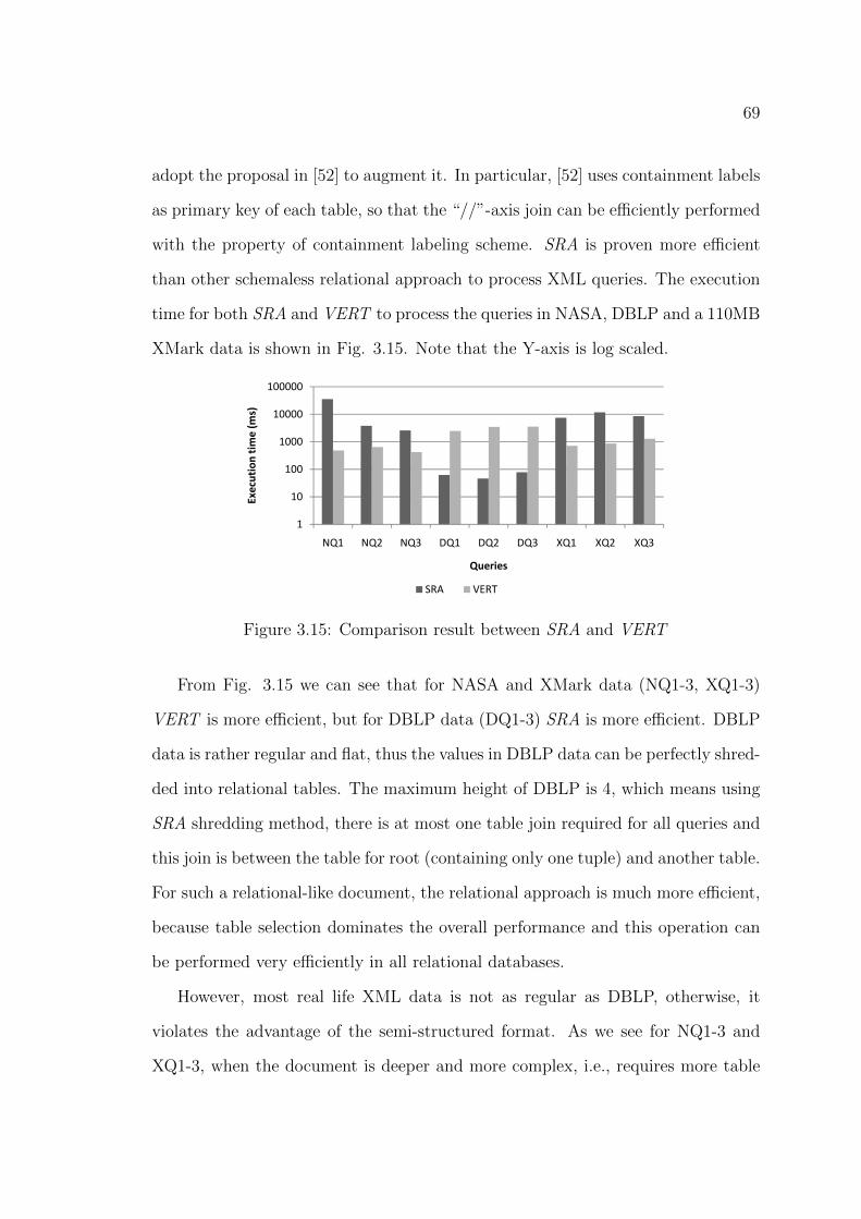
69

adopt the proposal in [52] to augment it. In particular, [52] uses containment labels

as primary key of each table, so that the “//”-axis join can be efficiently performed

with the property of containment labeling scheme. SRA is proven more efficient

than other schemaless relational approach to process XML queries. The execution

time for both SRA and VERT to process the queries in NASA, DBLP and a 110MB

XMark data is shown in Fig. 3.15. Note that the Y-axis is log scaled.

10000

100000

(ms)

100

1000

10000

100000

tion

time (m

s)

10

100

1000

10000

100000

Execution time (m

s)

1

10

100

1000

10000

100000

NQ1 NQ2 NQ3 DQ1 DQ2 DQ3 XQ1 XQ2 XQ3

Execution time (m

s)

Queries

1

10

100

1000

10000

100000


Execution time (m

s)

Queries

SRA VERT

1

10

100

1000

10000

100000


Execution time (m

s)

Queries

SRA VERT

1

10

100

1000

10000

100000


Execution time (m

s)

Queries

SRA VERT

Figure 3.15: Comparison result between SRA and VERT

From Fig. 3.15 we can see that for NASA and XMark data (NQ1-3, XQ1-3)

VERT is more efficient, but for DBLP data (DQ1-3) SRA is more efficient. DBLP

data is rather regular and flat, thus the values in DBLP data can be perfectly shred-

ded into relational tables. The maximum height of DBLP is 4, which means using

SRA shredding method, there is at most one table join required for all queries and

this join is between the table for root (containing only one tuple) and another table.

For such a relational-like document, the relational approach is much more efficient,

because table selection dominates the overall performance and this operation can

be performed very efficiently in all relational databases.

However, most real life XML data is not as regular as DBLP, otherwise, it

violates the advantage of the semi-structured format. As we see for NQ1-3 and

XQ1-3, when the document is deeper and more complex, i.e., requires more table

70

joins for SRA, the performance of SRA is badly affected.

In a word, the relational approach to process XML queries is only suitable for

regular XML documents, but not as good as structural join based approaches for

complex XML structures.

3.5.3 Comparison with TwigStack

Now we compare VERT with TwigStack, which is a typical structural join based

twig pattern matching algorithm. We test on two aspects, space management and

query performance.

Space management

As mentioned earlier, TwigStack does not specially handle value nodes during doc-

ument parsing and query processing, but treat them the same as other internal

nodes. There may be too many inverted lists, most of which contain very few

labels. In this part, we test the required space in document parsing, including

the number of labeled nodes in memory, and the number of inverted lists to be

managed. We parse the two real-world data sets, NASA and DBLP, and a 110MB

XMark data using TwigStack and VERT separately. The number of labeled nodes

and the number of inverted lists in the two approaches are shown in Fig. 3.16.

book

title

author



“White”

35 15author

“Brown”

authors

book



author

“Brown”

basicInfo saleInfo

Data Set Query Path Expression

NASA

NQ1 //dataset//source//other[date/year>1919 and year<2000]/author/lastName

NQ2 //dataset/tableHead[//field/name=‘rah’]//tableLinks //title

NQ3 //dataset//history//ingest[date[year>1949 and year<2000] [month=‘Nov’][day>14 and day<21]]//creator/lastName

DBLP

DQ1 /dblp/article[/author=‘Jim Gray’]/title

DQ2 /dblp/proceedings[year>1979]/isbn

DQ3/dblp/inproceedings[title=‘A Flexible Modeling Approach for Software Reliability Growth’][year=‘1987’][author=‘Sergio Bittanti’]/booktitle

XMark

XQ1 //regions/africa/item[//mailbox//mail/from=‘Libero Rive’]//keyword

XQ2 //person[//profile/age>20]/name

XQ3 //open_auction[//bidder[time>18:00:00]/increase>5]/quantity

Data SetNumber of Labeled Nodes Number of Inverted Lists

TwigStack VERT Saving

997,987 532,963 46.6%

6,771,148 3,736,406 44.8%

3,221,925 2,048,193 36.4%

NASA

DBLP

XMark

TwigStack VERT

121,833 68

388,630 37

353,476 79

Figure 3.16: Number of labeled nodes and inverted lists in TwigStack and VERT

71

This result validates our analysis in Section 3.2.5 about the reduction of labeled

nodes in memory and the reduction of inverted lists. In VERT, values are stored

in relational tables and the relational tables are built based on different types of

properties, so the number of tables is limited to the number of different property

types. There is no problem to manage the tables. We also use 10 sets of Xmark

data, whose sizes vary between 11MB and 110MB, to further prove the superiority

of VERT in space management. The experimental result is shown in Fig. 3.17.

We can see from the result that the number of labeled nodes is scaled to the

document size for both approaches, and VERT always manages less labeled nodes.

Furthermore, the number of inverted lists is scaled to the size of document in

TwigStack, whereas this number is a constant in VERT. For a large data set it is

not practical to handle the tremendous number of inverted lists using TwigStack.

No. of Nod No. of Streams No. of Node No. of Streams1 0.324273 0.072371 0.20613 7.9E-05 11.32 0.650335 0.124502 0.413111 7.9E-05 22.83 0.969617 0.164237 0.616229 7.9E-05 344 1.305245 0.208709 0.820438 7.9E-05 45.35 1.628549 0.239532 1.024073 7.9E-05 56.26 1 9634 0 267772 1 233723 7 9E 05 68 22.5

3

3.5

llion

)

6 1.9634 0.267772 1.233723 7.9E-05 68.27 2.294327 0.291727 1.440674 7.9E-05 79.78 2.61591 0.311866 1.643495 7.9E-05 90.79 2.943522 0.332839 1.849449 7.9E-05 102

10 3.221925 0.353476 2.048193 7.9E-05 111

1

1.5

2

2.5

3

3.5

ed n

odes

(Mill

ion)

1200Q1 year Q2 name Q3 year Q3 month Q3 day Q4 author Q5 year Q6 title Q6 year Q6 author Q7 from Q8Q9 loQ9 dQ9 to

TwigStack 71.58 874.656 71.58 29.436 29.436 8597.856 3945.972 3946.332 3945.972 8597.856 263.592 # 261 ## 263.352VERT 60.876 17.22 60.732 2.148 14.196 12.35 894.492 12 78.324 12 12 # 70 12 12

0

0.5

1

1.5

2

2.5

3

3.5

11 3 22 8 34 45 3 56 2 68 2 79 7 90 7 102 111

No.

of l

abel

ed n

odes

(Mill

ion)

800

1000

1200

(MB

)

8000

9000

0

0.5

1

1.5

2

2.5

3

3.5

11.3 22.8 34 45.3 56.2 68.2 79.7 90.7 102 111

No.

of l

abel

ed n

odes

(Mill

ion)

File size (MB)TwigStack VERT

200

400

600

800

1000

1200

Stre

am s

ize

(MB

)

800 200

250

300

B)

Q1 date Q2 filed Q3 date Q4 article Q5 proce Q6 inproce Q7 mail Q8 mail Q9 mailTwigStack 73.164 729.12 73.164 1339.308 36.084 2547.276 251.424 251.424 251.424optimizatio 60.732 17.22 5.208 12 10.98 12 36 50.42 12

5000

6000

7000

8000

9000

size

(MB

)

2500

3000

700

800

900

0

0.5

1

1.5

2

2.5

3

3.5

11.3 22.8 34 45.3 56.2 68.2 79.7 90.7 102 111

No.

of l

abel

ed n

odes

(Mill

ion)


0

200

400

600

800

1000

1200

Q7 from Q8 d

Stre

am s

ize

(MB

)

Str600

800

e (M

B)

100

150

200

250

300

Stre

am s

ize

(MB

)

0.3

0.35

0.4

ion)

2000

3000

4000

5000

6000

7000

8000

9000

Stre

am s

ize

(MB

)

1500

2000

2500

3000

m s

ize

(MB

)

400

500

600

700

800

900

am s

ize

(MB

)

0

0.5

1

1.5

2

2.5

3

3.5

11.3 22.8 34 45.3 56.2 68.2 79.7 90.7 102 111

No.

of l

abel

ed n

odes

(Mill

ion)


0

200

400

600

800

1000

1200

Q7 from Q8 d

Stre

am s

ize

(MB

)

Str

400

600

800

Stre

am s

ize

(MB

)

0

50

100

150

200

250

300

Stre

am s

ize

(MB

)

0.2

0.25

0.3

0.35

0.4

lists

(Million)

(a) Number of labeled nodes

No. of Nod No. of Streams No. of Node No. of Streams1 0.324273 0.072371 0.20613 7.9E-05 11.32 0.650335 0.124502 0.413111 7.9E-05 22.83 0.969617 0.164237 0.616229 7.9E-05 344 1.305245 0.208709 0.820438 7.9E-05 45.35 1.628549 0.239532 1.024073 7.9E-05 56.26 1 9634 0 267772 1 233723 7 9E 05 68 2

0.3

0.35

0.4

illion)

6 1.9634 0.267772 1.233723 7.9E-05 68.27 2.294327 0.291727 1.440674 7.9E-05 79.78 2.61591 0.311866 1.643495 7.9E-05 90.79 2.943522 0.332839 1.849449 7.9E-05 102

10 3.221925 0.353476 2.048193 7.9E-05 111

1200

0.15

0.2

0.25

0.3

0.35

0.4

verted

list

s(M

illion)

Q1 year Q2 name Q3 year Q3 month Q3 day Q4 author Q5 year Q6 title Q6 year Q6 author Q7 from Q8Q9 loQ9 dQ9 toTwigStack 71.58 874.656 71.58 29.436 29.436 8597.856 3945.972 3946.332 3945.972 8597.856 263.592 # 261 ## 263.352VERT 60.876 17.22 60.732 2.148 14.196 12.35 894.492 12 78.324 12 12 # 70 12 12

800

1000

1200

(MB

)0

0.05

0.1

0.15

0.2

0.25

0.3

0.35

0.4

11 3 22 8 34 45 3 56 2 68 2 79 7 90 7 102 111

No. of inverted

lists

(Million)

8000

9000200

400

600

800

1000

1200

Stre

am s

ize

(MB

)

800 200

250

300

B)

0

0.05

0.1

0.15

0.2

0.25

0.3

0.35

0.4

11.3 22.8 34 45.3 56.2 68.2 79.7 90.7 102 111

No. of inverted

lists

(Million)


Q1 date Q2 filed Q3 date Q4 article Q5 proce Q6 inproce Q7 mail Q8 mail Q9 mailTwigStack 73.164 729.12 73.164 1339.308 36.084 2547.276 251.424 251.424 251.424optimizatio 60.732 17.22 5.208 12 10.98 12 36 50.42 12

5000

6000

7000

8000

9000

size

(MB

)

2500

3000

700

800

900

3

3.5

n)

0

200

400

600

800

1000

1200

Q7 from Q8 d

Stre

am s

ize

(MB

)

Str600

800

e (M

B)

100

150

200

250

300

Stre

am s

ize

(MB

)

0

0.05

0.1

0.15

0.2

0.25

0.3

0.35

0.4

11.3 22.8 34 45.3 56.2 68.2 79.7 90.7 102 111

No. of inverted

lists

(Million)


2000

3000

4000

5000

6000

7000

8000

9000

Stre

am s

ize

(MB

)

1500

2000

2500

3000

m s

ize

(MB

)

400

500

600

700

800

900

am s

ize

(MB

)

2

2.5

3

3.5

es (M

illio

n)

0

200

400

600

800

1000

1200

Q7 from Q8 d

Stre

am s

ize

(MB

)

Str

400

600

800

Stre

am s

ize

(MB

)

0

50

100

150

200

250

300

Stre

am s

ize

(MB

)

0

0.05

0.1

0.15

0.2

0.25

0.3

0.35

0.4

11.3 22.8 34 45.3 56.2 68.2 79.7 90.7 102 111

No. of inverted

lists

(Million)


(b) Number of inverted lists

Figure 3.17: Space management comparisons

Query performance

We used NASA, DBLP and a 110MB XMark data set to compare the query pro-

cessing performance between TwigStack and our algorithms. The implementation

72

of TwigStack adopts B+ tree to index inverted lists, which ensures a high perfor-

mance of inverted list access for different values. We compare TwigStack with our

original VERT algorithm, as well as VERT Optimization 1 and Optimization 2.

As mentioned earlier, we can infer the object information in an XML document.

Although the inference may not be semantically correct, it will not affect the cor-

rectness of the result. In the two optimizations, we use such inference to construct

object/property tables and object tables. Since relationship information is not easy

to discovered without designer’s declaration, we do not test Optimization 3. The

execution time of VERT and its optimizations includes the I/O and CPU costs to

access relational tables to perform content search, the cost to construct temporary

inverted lists, and the cost on structural search. The comparison result is shown

in Fig. 3.18.

From the result we can see that for all queries, VERT outperforms TwigStack.

The reason is VERT performs content search first to simplify the query pattern

before structural joins, thus gains better overall performance. The result also proves

that the overhead on table selection will not affect the benefit gained from twig

pattern simplification. TwigStack performs very badly on DQ2. In the DBLP

data, there are a lot of numeric values. To process DQ2, TwigStack has to combine

the labels in all the inverted lists with a number name greater than 1979, based

on document order. To load and merge these inverted lists is costly. However,

in VERT this step is replaced by table selection, thus it is more efficient. We

can see, though for small document (e.g., NASA), TwigStack is not very slow to

perform range search, when the amount of labels in numeric inverted lists is large,

TwigStack will be inefficient to load and merge the labels.

For all the queries, Optimization 1 works better than VERT. The reason is

that Optimization 1 reduces one more level up to the original twig pattern query.

73

NASArelational twigstack vert opt1 opt2 sql

NQ1 //dataset//source/ 35495 640 485 406 407 select authoNQ2 //dataset/tableHea 3813 812 641 359 359 select tableNQ3 //dataset//history/ 2578 609 422 360 172 select creatDQ1 /dblp/article[/auth 62 2922 2453 1499 1578 select articlDQ2 /dblp/proceedings 46 15547 3454 2686 2752 select proceDQ3 /dblp/inproceeding 78 4132 3546 1623 1172 select inproXQ1 //regions/africa/ite 7421 789 713 640 671 select keywXQ2 //person[//profile/ 11730 1000 869 813 820 select persoXQ3 //open_auction[//b 8500 1716 1293 672 484 select open

100

1000

10000

100000

ecution time (m

s)

0

200

400

600

800

1000

NQ1 NQ2 NQ3

Execution time (m

s)

Query

TwigStack VERT

VERT Optimization 1 VERT Optimization 2

3000

6000

9000

12000

15000

18000

Execution time (m

s)

800

1200

1600

2000

xecution

time (m

s)

1

10

100

1000

10000

100000


Execution time (m

s)

Queries

SRA VERT

0

200

400

600

800

1000

NQ1 NQ2 NQ3

Execution time (m

s)

Query

TwigStack VERT


0

3000

6000

9000

12000

15000

18000

DQ1 DQ2 DQ3

Execution time (m

s)

Query

TwigStack VERT


0

400

800

1200

1600

2000

XQ1 XQ2 XQ3

Execution time (m

s)

Query

TwigStack VERT


(a) NASA

NASArelational twigstack vert opt1 opt2 sql

NQ1 //dataset//source/ 35495 640 485 406 407 select authoNQ2 //dataset/tableHea 3813 812 641 359 359 select tableNQ3 //dataset//history/ 2578 609 422 360 172 select creatDQ1 /dblp/article[/auth 62 2922 2453 1499 1578 select articlDQ2 /dblp/proceedings 46 15547 3454 2686 2752 select proceDQ3 /dblp/inproceeding 78 4132 3546 1623 1172 select inproXQ1 //regions/africa/ite 7421 789 713 640 671 select keywXQ2 //person[//profile/ 11730 1000 869 813 820 select persoXQ3 //open_auction[//b 8500 1716 1293 672 484 select open

100

1000

10000

100000

ecution time (m

s)200

400

600

800

1000

Execution time (m

s)

0

3000

6000

9000

12000

15000

18000

DQ1 DQ2 DQ3

Execution time (m

s)

Query

TwigStack VERT


400

800

1200

1600

2000

Execution time (m

s)

1

10

100

1000

10000

100000


Execution time (m

s)

Queries

SRA VERT

0

200

400

600

800

1000

NQ1

Execution time (m

s)

TwigStack

TwigTable Optimi

0

3000

6000

9000

12000

15000

18000

DQ1 DQ2 DQ3

Execution time (m

s)

Query

TwigStack VERT


0

400

800

1200

1600

2000

XQ1 XQ2 XQ3Execution time (m

s)Query

TwigStack TwigTable

TwigTable Optimization 1 TwigTable Optimization 2

(b) DBLPNASA

relational twigstack vert opt1 opt2 sqlNQ1 //dataset//source/ 35495 640 485 406 407 select authoNQ2 //dataset/tableHea 3813 812 641 359 359 select tableNQ3 //dataset//history/ 2578 609 422 360 172 select creatDQ1 /dblp/article[/auth 62 2922 2453 1499 1578 select articlDQ2 /dblp/proceedings 46 15547 3454 2686 2752 select proceDQ3 /dblp/inproceeding 78 4132 3546 1623 1172 select inproXQ1 //regions/africa/ite 7421 789 713 640 671 select keywXQ2 //person[//profile/ 11730 1000 869 813 820 select persoXQ3 //open_auction[//b 8500 1716 1293 672 484 select open

100

1000

10000

100000

ecution time (m

s)

200

400

600

800

1000

Execution time (m

s)

3000

6000

9000

12000

15000

18000

Execution time (m

s)

0

400

800

1200

1600

2000

XQ1 XQ2 XQ3

Execution time (m

s)

Query

TwigStack VERT


1

10

100

1000

10000

100000


Execution time (m

s)

Queries

SRA VERT

0

200

400

600

800

1000

NQ1

Execution time (m

s)

TwigStack

TwigTable Optimi

0

3000

6000

9000

12000

15000

18000

DQ1 DQ2 DQ3

Execution time (m

s)

Query

TwigStack VERT


0

400

800

1200

1600

2000

XQ1 XQ2 XQ3

Execution time (m

s)

Query

TwigStack VERT


(c) XMark

Figure 3.18: Execution time by TwigStack and VERT without optimizations, withOptimization 1 and with Optimization 2 in the three XML documents

Similarly, the query processing performance is further improved.

Comparing Optimization 1 with Optimization 2, we can see that for single-

predicated queries there is no obvious difference. For some queries, Optimization 2

is even slightly worse than Optimization 1. The reason is that the combined object

table is larger than object/property table, and then there may be more I/Os to

load tuples for object table. However, for multi-predicated queries, e.g., the queries

Q3, Q6 and Q9, Optimization 2 has a better performance, because Optimization

2 performs content search for all the value comparisons on the same object at the

same time. This again proves our analysis in Section 3.2.5.

74

3.6 Summary

In this chapter, we propose a semantic approach VERT to solve different kinds

of content problems raised in existing approaches for twig pattern query process-

ing. Unlike TwigStack and its subsequent algorithms, our approach uses semantic

tables to store values in XML document and avoids the management of tremen-

dous number inverted lists for different values. Query processing in our approach

is done by performing content search first to reduce the size of relevant inverted

lists, rewriting twig pattern queries to reduce the number of structural nodes and

the number of structural joins for structural search, and matching the simplified

pattern with reduced inverted lists to the document.

Our approach is a semantic approach because the relational tables are initially

built based on the semantics of property. With more semantics on objects and

relationships, we propose three optimizations to further improve the tables and en-

hance efficiency of query processing. In particular, if the relationship between ob-

ject and property is known, we can optimize the property table to object/property

table; if we know certain properties belong to the same object, we can combine

the object/property tables to be object table; if the relationship between objects

is known, we can introduce relationship tables to precisely store the property val-

ues of relationships. Furthermore, after finding an occurrence of a twig pattern

in the document in terms of labels, our algorithm can easily extract actual value

to answer the query from relational tables if the output node is a property node;

whereas the previous approaches need more work to convert labels into values by

accessing documents again. Due to this advantage, our approach can easily bridge

the gap between pattern matching and value-based join for general XML queries

involving ID references and other types of value-based joins.

75

CHAPTER 4

ENHANCING TWIG PATTERN

SEMANTICS FOR COMPLEX

OUTPUT INFORMATION

Due to the limited expressivity of twig pattern expressions, many queries that

aim to find complex output information under one object have to be expressed in

several twig patterns linked by joins. Although our VERT algorithm proposed in

Chapter 3 can match and join multiple twig patterns for such a query, intuitively

it is redundant to do so because all the twig patterns for such a query are centered

on the same object and we may perform the same structural join multiple times

when matching different twig patterns.

In this chapter we analyze the characteristics of each query node, i.e., the pur-

pose, optionality and occurrence, and classify the nodes in a twig pattern query into

six types, namely, predicate node, optional-predicate node, output node, optional-

76

output node, predicated-output node, and optional-predicated-output node. Then

we propose the TP+Output expression to extend twig pattern queries, to model

complex output information based on the semantics of different node types. With

TP+Output, queries with a complex output can be expressed in fewer twig expres-

sions and processed by fewer structural joins in pattern matching. Last, we extend

the VERT algorithm as VERTO, to process the TP+Output query, and demon-

strate the performance improvement of using TP+Output to represent queries.

4.1 Introduction

As mentioned in Chapter 1, an XML document is normally modeled as a tree,

without considering ID references. Fig. 4.1 shows an example XML document

modeled as a tree with positional labels under the containment labeling scheme.

We refer to this document as the Company document in later examples. Also,

the core query pattern for a general XML query is a twig pattern or multiple twig

patterns linked by joins. Matching a twig pattern query to an XML document tree

is considered the main operation for XML query processing. In this chapter, we

focus on how the rich semantics of a query pattern impacts on the efficiency of

query processing.

There is a class of queries, which finds a particular object based on certain pred-

icates, and outputs complex information about that object. Such queries cannot

be expressed by a single twig pattern expression, because of the complexity of the

output. This class of queries have to be expressed using XQuery expressions which

match with more than one twig patterns. Fig. 4.2 shows some example queries

with complex output information from a unique object. All of them have simple,

or in some cases no predicate applied to the target object, but none of these queries

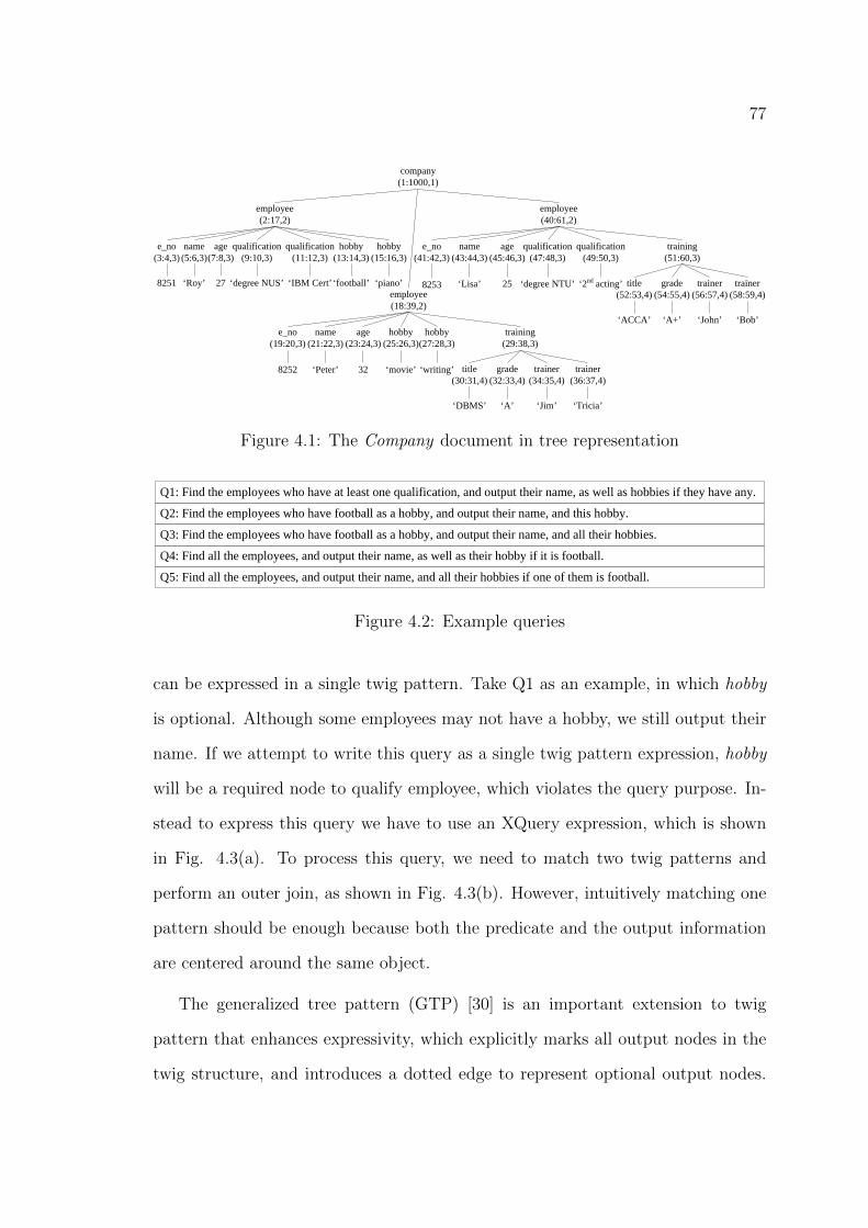
77

employee

name hobby

‘Roy’

employee

name hobbyqualification

employee


employee

name hobby

‘football’

“ER”

description?

XQ5closed_auction

“person8001”

seller buyer

item

“person11029”

price

XQ4open_auction

reserve

initial annotation quantity?

happiness?

XQ2person

name profileaddress

country

“Finland”

interest?

XQ1item

locatioin

“United States”

description

incategory?

“category48”

incategory

NQ1dataset

subject

“astronomy”

title reference?

NQ2reference

title

journal

author?

source

lastName

“Wu”

author

NQ4tableHead

tableLink

title

“MASOL”

field

name

fields

units?

DQ1article

author editor?title

“Frank Manola”

DQ3inproceedings

author titlebooktitle

“Wilfred Ng”

cite?

DQ5inproceedings

author cite?title

“Uwe Hohenstein”

cite

label

“Da 86”

DQ4proceedings

year titleISBN

“1999”

NQ3history

ingest

>1990 and <1994

year

date creator

lastName affiliation

NQ5dataset

altname

type

“ADC”

altname

XQ3person

profile watches

watch

“open_aunction7377”

age

18

watch

DQ2inproceedings

author authortitle

“Gerhard Mehlsam”

company(1:1000,1)

employee(2:17,2)

employee(40:61,2)

e_no(3:4,3)

age(7:8,3)

qualification(9:10,3)

name(5:6,3)

hobby(13:14,3)


8251 ‘Roy’ ‘degree NUS’27 ‘IBM Cert’ ‘football’

hobby(15:16,3)

‘piano’

e_no(41:42,3)

age(45:46,3)


name(43:44,3)

8253 ‘Lisa’ ‘degree NTU’25


‘2nd acting’

training(51:60,3)

title(52:53,4)

grade(54:55,4)

trainer(56:57,4)

trainer(58:59,4)

‘ACCA’ ‘A+’ ‘John’ ‘Bob’

employee(18:39,2)

e_no(19:20,3)

name(21:22,3)

hobby(25:26,3)

age(23:24,3)

8252 ‘Peter’ 32 ‘movie’

hobby(27:28,3)

‘writing’

training(29:38,3)

title(30:31,4)

grade(32:33,4)

trainer(34:35,4)

trainer(36:37,4)

‘DBMS’ ‘A’ ‘Jim’ ‘Tricia’

employee name(2:17,2) (5:6,3)

qualification hobby

(2:17,2) (5:6,3)(2:17,2) (5:6,3)(2:17,2) (5:6,3)(2:17,2) (5:6,3)(2:17,2) (5:6,3)

(7:8,3) (11:12,3)(7:8,3) (13:14,3)(7:8,3) (15:16,3)

(9:10,3) (11:12,3)(9:10,3) (13:14,3)(9:10,3) (15:16,3)

... ... ... ...

employee’

name age training’

title

Rewritten Twig

ListsL ---- (employee/name) (course/title)PL ---- (employee/age, >24) OL ---- (training/trainer) OPL---- (employee/hobby, movie, all)

Pattern Matching

employee name(18:39,2) (21:22,3)

age training(23:24,3) (29:38,3)

title(30:31,4)

Figure 4.1: The Company document in tree representation

XQ1: FOR $d IN doc("XMark.xml")//item[location="United States"]/incategory RETURN if ($d/@category="category48")

then (<category>$d/../incategory </category>) else ()XQ2: FOR $p IN doc("XMark.xml")//person[address/country="Finland"] RETURN <person>{<name>{$p/name}</name>,

<interest>{$p/profile/interest}</interest>}</person>XQ3:FOR $w IN doc("XMark.xml")//person[profile/age="18"]/watches WHERE $w/watch/@open_auction="open_auction7377" RETURN <watch>{$w/watch}</watch>XQ4:FOR $o IN doc("XMark.xml")//open_auction[reserve][annotation] LET $i:=$o/initial RETURN <auction>{$i, $o/annotation/happiness, $o/quantity}</auction>XQ5:FOR $c in doc("test.xml")//closed_auction[seller/@person="person8001"]

[buyer/@person="person1029"][itemref][price] RETURN <auction>{$c/itemref, $c/price, $c/description}</auction>

Q1: Find the employees who have at least one qualification, and output their name, as well as hobbies if they have any.

Q2: Find the employees who have football as a hobby, and output their name, and this hobby.

Q3: Find the employees who have football as a hobby, and output their name, and all their hobbies.

Q4: Find all the employees, and output their name, as well as their hobby if it is football.

Q5: Find all the employees, and output their name, and all their hobbies if one of them is football.

Figure 4.2: Example queries

can be expressed in a single twig pattern. Take Q1 as an example, in which hobby

is optional. Although some employees may not have a hobby, we still output their

name. If we attempt to write this query as a single twig pattern expression, hobby

will be a required node to qualify employee, which violates the query purpose. In-

stead to express this query we have to use an XQuery expression, which is shown

in Fig. 4.3(a). To process this query, we need to match two twig patterns and

perform an outer join, as shown in Fig. 4.3(b). However, intuitively matching one

pattern should be enough because both the predicate and the output information

are centered around the same object.

The generalized tree pattern (GTP) [30] is an important extension to twig

pattern that enhances expressivity, which explicitly marks all output nodes in the

twig structure, and introduces a dotted edge to represent optional output nodes.

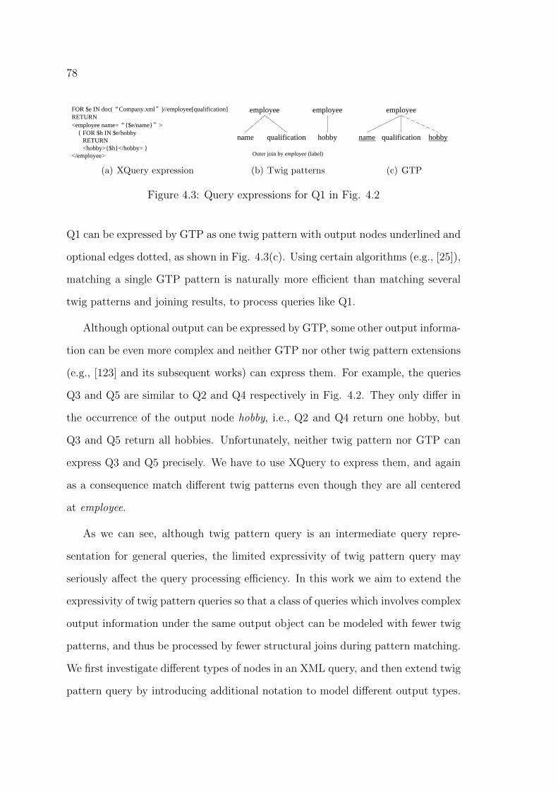
78

employee

name hobby

‘Roy’

employee


employee


employee

name hobby

‘football’

“ER”

description?

XQ5

closed_auction

“person8001”

seller buyer

item

“person11029”

price

XQ4

open_auction

reserve


happiness?

XQ2

person

name profileaddress

country

“Finland”

interest?

XQ1

item

locatioin

“United States”

description

incategory?

“category48”

incategory

NQ1

dataset

subject

“astronomy”

title reference?

NQ2

reference

title

journal

author?

source

lastName

“Wu”

author

NQ4

tableHead

tableLink

title

“MASOL”

field

name

fields

units?

DQ1

article

author editor?title

“Frank Manola”

DQ3

inproceedings


“Wilfred Ng”

cite?

DQ5

inproceedings

author cite?title


cite

label

“Da 86”

DQ4

proceedings

year titleISBN

“1999”

NQ3

history

ingest

>1990 and <1994

year

date creator


NQ5

dataset

altname

type

“ADC”

altname

XQ3

person

profile watches

watch


age

18

watch

DQ2

inproceedings

author authortitle


company(1:1000,1)

employee(2:17,2)

employee(40:61,2)

e_no(3:4,3)

age(7:8,3)


name(5:6,3)

hobby(13:14,3)


8251 ‘Roy’ ‘degree NUS’27 ‘IBM Cert’ ‘football’

hobby(15:16,3)

‘piano’

e_no(41:42,3)

age(45:46,3)


name(43:44,3)

8253 ‘Lisa’ ‘degree NTU’25


‘2nd acting’

training(51:60,3)

title(52:53,4)

grade(54:55,4)

trainer(56:57,4)

trainer(58:59,4)


employee(18:39,2)

e_no(19:20,3)

name(21:22,3)

hobby(25:26,3)

age(23:24,3)


hobby(27:28,3)

‘writing’

training(29:38,3)

title(30:31,4)

grade(32:33,4)

trainer(34:35,4)

trainer(36:37,4)


employee name

(2:17,2) (5:6,3)

qualification hobby

(2:17,2) (5:6,3)

(2:17,2) (5:6,3)

(2:17,2) (5:6,3)

(40:61,2) (43:44,3)

(40:61,2) (43:44,3)

(9:10,3) (13:14,3)

(9:10,3) (15:16,3)

(11:12,3) (13:14,3)

(11:12,3) (15:16,3)

(47:48,3) null

(49:50,3) null

employee’


title

Rewritten Twig

Lists

L ---- (employee/name) (course/title)

PL ---- (employee/age, >24)

OL ---- (training/trainer)

OPL---- (employee/hobby, movie, all)

Pattern Matching

employee name

(18:39,2) (21:22,3)

age training

(23:24,3) (29:38,3)

title

(30:31,4)

FOR $e IN doc(“Company.xml”)//employee[qualification]RETURN<employee name=“{$e/name}”> { FOR $h IN $e/hobby RETURN <hobby>{$h}</hobby> }</employee>

(a) XQuery expression

employee

name hobby

‘Roy’

employee

name hobby

‘football’

“ER”

description?

XQ5closed_auction

“person8001”

seller buyer

item

“person11029”

price

XQ4open_auction

reserve


happiness?

XQ2person

name profileaddress

country

“Finland”

interest?

XQ1item

locatioin

“United States”

description

incategory?

“category48”

incategory

NQ1dataset

subject

“astronomy”

title reference?

NQ2reference

title

journal

author?

source

lastName

“Wu”

author

NQ4tableHead

tableLink

title

“MASOL”

field

name

fields

units?

DQ1article

author editor?title

“Frank Manola”

DQ3inproceedings


“Wilfred Ng”

cite?

DQ5inproceedings

author cite?title


cite

label

“Da 86”

DQ4proceedings

year titleISBN

“1999”

NQ3history

ingest

>1990 and <1994

year

date creator


NQ5dataset

altname

type

“ADC”

altname

XQ3person

profile watches

watch


age

18

watch

DQ2inproceedings

author authortitle


office(1:1000,1)

employee(2:17,2)

employee(40:41,2)

e_no(3:4,3)

age(7:8,3)


name(5:6,3)

hobby(13:14,3)


8251 ‘Roy’ ‘degree NUS’27 ‘football’

hobby(15:16,3)

‘piano’

e_no(41:42,3)

age(45:46,3)


name(43:44,3)

8253 ‘Lisa’ ‘degree NTU’


‘2nd acting’

training(51:60,3)

title(52:53,4)

grade(54:55,4)

trainer(56:57,4)

trainer(58:59,4)

‘bidding’ ‘A+’ ‘John’ ‘Bob’

employee(18:39,2)

e_no(19:20,3)

name(21:22,3)

hobby(25:26,3)

age(23:24,3)


hobby(27:28,3)

‘writing’

training(29:38,3)

title(30:31,4)

grade(32:33,4)

trainer(34:35,4)

trainer(36:37,4)



qualification hobby

(2:17,2) (5:6,3)(2:17,2) (5:6,3)(2:17,2) (5:6,3)(2:17,2) (5:6,3)(2:17,2) (5:6,3)

(7:8,3) (11:12,3)(7:8,3) (13:14,3)(7:8,3) (15:16,3)

(9:10,3) (11:12,3)(9:10,3) (13:14,3)(9:10,3) (15:16,3)

... ... ... ...

Q1: Find the employees who have at lest one qualification, and output his name, as well as hobbies if he has.

Q2: Find the employees who have a hobby of football, and output his name and this hobby.

Q3: Find the employees who have a hobby of football, and output his name and all his hobbies.

Q4: Find all the employees, and output his name, as well as the hobby if it is football.

Q5: Find all the employees, and output his name and all his hobbies if one of them is football.

‘IBM Cert’ 25

employee


employee

Outer join by employee (label)

employee


(b) Twig patterns

employee

name hobby

‘Roy’

employee


employee

name hobby

‘football’

“ER”

description?

XQ5closed_auction

“person8001”

seller buyer

item

“person11029”

price

XQ4open_auction

reserve


happiness?

XQ2person

name profileaddress

country

“Finland”

interest?

XQ1item

locatioin

“United States”

description

incategory?

“category48”

incategory

NQ1dataset

subject

“astronomy”

title reference?

NQ2reference

title

journal

author?

source

lastName

“Wu”

author

NQ4tableHead

tableLink

title

“MASOL”

field

name

fields

units?

DQ1article

author editor?title

“Frank Manola”

DQ3inproceedings


“Wilfred Ng”

cite?

DQ5inproceedings

author cite?title


cite

label

“Da 86”

DQ4proceedings

year titleISBN

“1999”

NQ3history

ingest

>1990 and <1994

year

date creator


NQ5dataset

altname

type

“ADC”

altname

XQ3person

profile watches

watch


age

18

watch

DQ2inproceedings

author authortitle


office(1:1000,1)

employee(2:17,2)

employee(40:41,2)

e_no(3:4,3)

age(7:8,3)


name(5:6,3)

hobby(13:14,3)


8251 ‘Roy’ ‘degree NUS’27 ‘football’

hobby(15:16,3)

‘piano’

e_no(41:42,3)

age(45:46,3)


name(43:44,3)

8253 ‘Lisa’ ‘degree NTU’


‘2nd acting’

training(51:60,3)

title(52:53,4)

grade(54:55,4)

trainer(56:57,4)

trainer(58:59,4)

‘bidding’ ‘A+’ ‘John’ ‘Bob’

employee(18:39,2)

e_no(19:20,3)

name(21:22,3)

hobby(25:26,3)

age(23:24,3)


hobby(27:28,3)

‘writing’

training(29:38,3)

title(30:31,4)

grade(32:33,4)

trainer(34:35,4)

trainer(36:37,4)



qualification hobby

(2:17,2) (5:6,3)(2:17,2) (5:6,3)(2:17,2) (5:6,3)(2:17,2) (5:6,3)(2:17,2) (5:6,3)

(7:8,3) (11:12,3)(7:8,3) (13:14,3)(7:8,3) (15:16,3)

(9:10,3) (11:12,3)(9:10,3) (13:14,3)(9:10,3) (15:16,3)

... ... ... ...

Q1: Find the employees who have at lest one qualification, and output his name, as well as hobbies if he has.

Q2: Find the employees who have a hobby of football, and output his name and this hobby.

Q3: Find the employees who have a hobby of football, and output his name and all his hobbies.

Q4: Find all the employees, and output his name, as well as the hobby if it is football.

Q5: Find all the employees, and output his name and all his hobbies if one of them is football.

‘IBM Cert’ 25

employee


employee

Join two patterns by employee (label)

(c) GTP

Figure 4.3: Query expressions for Q1 in Fig. 4.2

Q1 can be expressed by GTP as one twig pattern with output nodes underlined and

optional edges dotted, as shown in Fig. 4.3(c). Using certain algorithms (e.g., [25]),

matching a single GTP pattern is naturally more efficient than matching several

twig patterns and joining results, to process queries like Q1.

Although optional output can be expressed by GTP, some other output informa-

tion can be even more complex and neither GTP nor other twig pattern extensions

(e.g., [123] and its subsequent works) can express them. For example, the queries

Q3 and Q5 are similar to Q2 and Q4 respectively in Fig. 4.2. They only differ in

the occurrence of the output node hobby, i.e., Q2 and Q4 return one hobby, but

Q3 and Q5 return all hobbies. Unfortunately, neither twig pattern nor GTP can

express Q3 and Q5 precisely. We have to use XQuery to express them, and again

as a consequence match different twig patterns even though they are all centered

at employee.

As we can see, although twig pattern query is an intermediate query repre-

sentation for general queries, the limited expressivity of twig pattern query may

seriously affect the query processing efficiency. In this work we aim to extend the

expressivity of twig pattern queries so that a class of queries which involves complex

output information under the same output object can be modeled with fewer twig

patterns, and thus be processed by fewer structural joins during pattern matching.

We first investigate different types of nodes in an XML query, and then extend twig

pattern query by introducing additional notation to model different output types.

79

The contributions of this chapter can be summarized as follows:

• Analyze the characteristics of query nodes, which leads to the classifica-

tion of query nodes: predicate nodes, optional-predicate nodes, output nodes,

optional-output nodes, predicated-output nodes and optional-predicated-output

nodes.

• Extend twig pattern queries with notation to explicitly mark different types

of output nodes. We call the extended twig pattern TP+Output.

• Extend our previous query processing algorithm, VERT to VERTO, to pro-

cess TP+Output queries.

• Conduct experiments to compare the query processing performance between

TP+Output, the original twig pattern representation, and two typical XQuery

processors, to verify the performance improvement of using TP+Output.

The rest of this chapter is arranged as follows. Section 4.2 analyzes the char-

acteristics of query nodes and Section 4.3 presents TP+Output, our extension to

the twig pattern query. Section 4.4 provides our extension VERTO, to process

TP+Output queries. Finally, Section 4.5 describes our experimental results and

Section 4.6 summarizes this chapter.

4.2 Query node characteristics

In this section, we analyze the characteristics of each node in a twig pattern query

in three aspects: the purpose, the optionality and the occurrence.

80

4.2.1 Purpose of query nodes

Normally an XML query aims to return some information based on certain condi-

tions. As a result, in an XML twig pattern query, some nodes represent conditions,

while some nodes represent information to be returned. In a twig pattern query,

if a query node specifies some constraints to filter the results, we say this node is

for predicate purpose. Contrarily, if a query node specifies what information the

query needs to return, we say this node is for output purpose.

Consider the query Q1 in the GTP representation in Fig. 4.3(c). Nodes em-

ployee and qualification are used to specify the structural constraint of the query,

so they are for predicate purpose, while nodes name and hobby are for output pur-

pose. However, there is a case that some query nodes are for both predicate and

output purposes. Consider a query to find the names of all employees with age

greater than 30, and also output the age. In this query, age plays a predicate role,

as it specifies a selection condition; and it also plays an output role, as we need to

return its value. Finally, we classify the purpose of nodes in a twig pattern query

into predicate, output and predicated-output.

4.2.2 Optionality of query nodes

The existence of a query node can be either required or optional. We start from

the optionality of predicate node. A predicate node specifying selection condition

of a query is normally required. For example in Q1, the predicate node qualification

must be matched in every qualified answer. In some cases, predicate node can also

be optional. Suppose we change the condition of Q1 to be the employee whose

qualification is “IBM Cert” if he has any (i.e., either have no qualification or have

qualification of “IBM Cert”). Then the qualification node becomes an optional

predicate node.

81

Now we focus on the output information. Output node and predicated-output

node in twig pattern query can be either required or optional. In Q1 name is

required output information, but hobby is optional. If a qualified employee has

certain hobbies, we output them alongside his name; otherwise, we just output his

name with an empty set of hobbies.

Similarly, the predicated-output node is either required or optional. The query

Q2 and Q4 in Fig. 4.2 both involve predicated-output nodes, but differ on the

optionality of the predicated-output node. In Q2, hobby is required to qualify an

employee. However in Q4, hobby is optional, i.e., we do not qualify an employee

based on hobby. If the hobby football exists for a qualified employee, we will output

it; otherwise no hobby is output for the qualified employee.

4.2.3 Occurrence of output information

Predicate node is not constrained by the occurrence of the node. In other words,

as long as one document node matches a predicate node, the predicate is satisfied.

However, the occurrence of output information may vary with query purpose, when

the node corresponds to a multi-valued element. We discuss the occurrence of

output node and predicated-output node as follows.

In an XML document, an element or attribute can be either single-valued or

multi-valued with respect to its parent element. For example, in the Company

document, e no, name and age are single-valued with respect to employee, but

qualification and hobby are multi-valued with respect to employee.

The occurrence of an output node is always many. When the corresponding

document node is single-valued, the target value is outputted; while when the

corresponding document node is multi-valued, all values must be outputted. For

example, if both name and hobby are output nodes in a twig pattern query, for

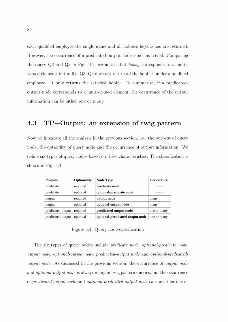
82

each qualified employee the single name and all hobbies he/she has are returned.

However, the occurrence of a predicated-output node is not as trivial. Comparing

the query Q2 and Q3 in Fig. 4.2, we notice that hobby corresponds to a multi-

valued element; but unlike Q3, Q2 does not return all the hobbies under a qualified

employee. It only returns the satisfied hobby. To summarize, if a predicated-

output node corresponds to a multi-valued element, the occurrence of the output

information can be either one or many.

4.3 TP+Output: an extension of twig pattern

Now we integrate all the analysis in the previous section, i.e., the purpose of query

node, the optionlity of query node and the occurrence of output information. We

define six types of query nodes based on these characteristics. The classification is

shown in Fig. 4.4.










Purpose

predicate

predicate

output

output

predicated-output

predicated-output

Optionality

required

optional

required

optional

required

optional

Node Type

predicate node

optional-predicate node

output node

optional-output node

predicated-output node

optional-predicated-output node

Occurrence

many

many

one or many

one or many

Figure 4.4: Query node classification

The six types of query nodes include predicate node, optional-predicate node,

output node, optional-output node, predicated-output node and optional-predicated-

output node. As discussed in the previous section, the occurrence of output node

and optional-output node is always many in twig pattern queries, but the occurrence

of predicated-output node and optional-predicated-output node can be either one or

83

many.

We first define the TP+Output query, which is an extension of twig pattern

query.

Definition 4.1. A TP+Output query is TPO = (( n, L)∗, (es | ed)∗). n is a query

node with the same semantics as that in the original twig pattern query. L is a set

of labels associated to the query node n, where L ⊆ {?, , →n}. In particular, a

query node n may be marked as optional (“?”), output (“ ”), and the occurrence

of many (“→n”). es and ed stand for solid edge and dotted edge respectively.

Now we formally define each type of query node, and present how to use the

TP+Output to express queries with these node types.

4.3.1 Predicate node

Definition 4.2. In a twig pattern query, if certain nodes specify either a structural

constraint or a value constraint, and the existence of these nodes is required, then

these nodes are called predicate nodes.

It is quite often that an XML query involves value comparisons on certain query

nodes. Obviously those value comparisons, together with their parent query nodes,

are predicate nodes. The node hobby and ‘football’ in the query in Fig. 4.5(a)

are both predicate node. Now we show another case of predicate node, where no

value comparison is involved. Consider the twig pattern representation for Q1 in

Fig. 4.6(a) (ignoring additional notation). In this query, qualification is not for

output purpose, but specifies a selection constraint. Although it does not have any

child value comparison, we still consider it as a predicate node. In TP+Output

extension, the nodes without any special labels are all predicate nodes.

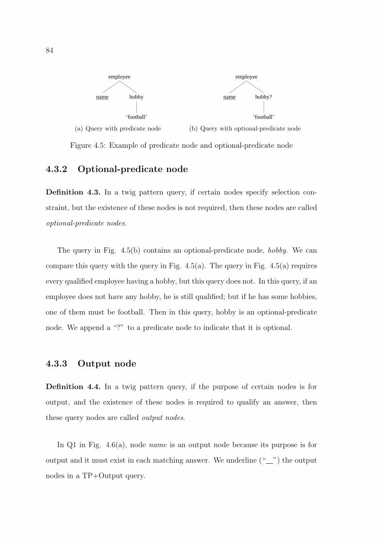
84XQ1: FOR $d IN doc("XMark.xml")//item[location="United States"]/incategory RETURN if ($d/@category="category48")









Purpose

predicate

predicate

output

output

predicated-output

predicated-output

Optionality

required

optional

required

optional

required

optional

Node Type

predicate node


output node




Occurrence

many

many

one or many

one or many

employee

‘football’

hobbyname

(a) Query with predicate node










Purpose

predicate

predicate

output

output

predicated-output

predicated-output

Optionality

required

optional

required

optional

required

optional

Node Type

predicate node


output node




Occurrence

many

many

one or many

one or many

employee

‘football’

hobby?name

(b) Query with optional-predicate node

Figure 4.5: Example of predicate node and optional-predicate node

4.3.2 Optional-predicate node

Definition 4.3. In a twig pattern query, if certain nodes specify selection con-

straint, but the existence of these nodes is not required, then these nodes are called

optional-predicate nodes.

The query in Fig. 4.5(b) contains an optional-predicate node, hobby. We can

compare this query with the query in Fig. 4.5(a). The query in Fig. 4.5(a) requires

every qualified employee having a hobby, but this query does not. In this query, if an

employee does not have any hobby, he is still qualified; but if he has some hobbies,

one of them must be football. Then in this query, hobby is an optional-predicate

node. We append a “?” to a predicate node to indicate that it is optional.

4.3.3 Output node

Definition 4.4. In a twig pattern query, if the purpose of certain nodes is for

output, and the existence of these nodes is required to qualify an answer, then

these query nodes are called output nodes.

In Q1 in Fig. 4.6(a), node name is an output node because its purpose is for

output and it must exist in each matching answer. We underline (“ ”) the output

nodes in a TP+Output query.

85

office

employee employee

ID qualification qualificationname hobbyhobby

‘24’ ‘Roy’ ‘IBM Cert’‘degree NUS’ ‘football’ ‘PS2’

hobby

‘piano’

ID qualification qualificationname

‘26’ ‘Lisa’ ‘1st singing’‘degree NTU’

qualification

‘2nd acting’

course

title grade lecturer lecturer


employee

ID name hobbyhobby

‘25’ ‘Peter’ ‘basketball’‘movie’

hobby

‘writing’

course



course

title lecturer

‘CFA’ ‘Mark’

employee

name hobby

‘Roy’

employee

name

for $e in doc(“office.xml”)//employeelet $hobby:=$e/hobbylet $qualification:=$e/qualificationreturn

<employee>{$e/name}{$hobby}{$qualification}

</employee>

employee

hobby

Find the name of the employees who have a hobby of football, and output the name and all the hobbies he/she has

Find the employees who have an ID greater than 24 and have at least one hobby, and output his/her ID, name, as well as the qualifications if any

office(0:67,1)

employee(1:16,2)

ID(2:3,3)



name(4:5,3)

hobby(12:13,3)

hobby(10:11,3)


hobby(14:15,3)

‘piano’

...

employee

[hobby]name course

Find names of employees who have completed some course (thus given a grade) together with the completed course’s title, and lecturers, if any

[grade]title lecturer?

E1.1 (NASA)

dataset

source

other

date

year

>1999 & <2000

author

lastName

E1.2 (NASA)

dataset

source

other

date

year

>1999 & <2000

author

initial

E1.3 (NASA)

dataset

source

other

date

year

>1999 & <2000

author

suffix

E1 (NASA)

dataset

source

other

date

year

>1999 & <2000

author

lastName initial? suffix?

E2.1 (NASA)

dataset

reference

author

subject

suffix initial

‘W’

E2.2 (NASA)

dataset

reference

author

subject

lastName initial

‘W’

suffix?

E2 (NASA)

dataset

reference

author

subject

lastName initial

‘W’

suffix

E3.1 (NASA)

dataset

reference

author

subject

lastName initial

‘W’

[suffix]

E3 (NASA)

dataset

reference

author

subject

lastName initial

‘W’

E4.1 (STOCKS)

Day

remarks

‘CD’

volume date bid closing

‘2007-11-30’

E4 (STOCKS)

Day

remarks

‘CD’

[volume] date [bid] closing

‘2007-11-30’

E5 (STOCKS)

Stock

code

‘500’

security Day

date

‘2007-11-30’high low

[closing]

changevolume?

bid?offer?

[opening]

currency?valueOf?

employee

ID name

>24

‘football’

employee

hobbyname course


ID

>24

hobby

“movie”

hobbyname

Find the employees who have at least one qualification, and output the name, as well as the hobbies if he/she has

hobby?qualification

(a) Q1

office

employee employee



hobby

‘piano’



qualification

‘2nd acting’

course



employee

ID name hobbyhobby


hobby

‘writing’

course



course

title lecturer


employee

name hobby

‘Roy’

employee

name hobby



</employee>

employee

hobby



office(0:67,1)

employee(1:16,2)

ID(2:3,3)



name(4:5,3)

hobby(12:13,3)

hobby(10:11,3)


hobby(14:15,3)

‘piano’

...

employee

[hobby]name course



E1.1 (NASA)

dataset

source

other

date

year

>1999 & <2000

author

lastName

E1.2 (NASA)

dataset

source

other

date

year

>1999 & <2000

author

initial

E1.3 (NASA)

dataset

source

other

date

year

>1999 & <2000

author

suffix

E1 (NASA)

dataset

source

other

date

year

>1999 & <2000

author


E2.1 (NASA)

dataset

reference

author

subject

suffix initial

‘W’

E2.2 (NASA)

dataset

reference

author

subject

lastName initial

‘W’

suffix?

E2 (NASA)

dataset

reference

author

subject

lastName initial

‘W’

suffix

E3.1 (NASA)

dataset

reference

author

subject

lastName initial

‘W’

[suffix]

E3 (NASA)

dataset

reference

author

subject

lastName initial

‘W’

E4.1 (STOCKS)

Day

remarks

‘CD’


‘2007-11-30’

E4 (STOCKS)

Day

remarks

‘CD’


‘2007-11-30’

E5 (STOCKS)

Stock

code

‘500’

security Day

date

‘2007-11-30’high low

[closing]

changevolume?

bid?offer?

[opening]

currency?valueOf?

employee

ID name

>24

‘football’

employee

hobbyname course


ID

>24

hobby

“movie”

hobbyname

Find the name of the employees who have a hobby of football, and output this hobby

‘football’

(b) Q2

office

employee employee



hobby

‘piano’



qualification

‘2nd acting’

course



employee

ID name hobbyhobby


hobby

‘writing’

course



course

title lecturer


employee

name hobby

‘Roy’

employee

name



</employee>

employee

hobby



office(0:67,1)

employee(1:16,2)

ID(2:3,3)



name(4:5,3)

hobby(12:13,3)

hobby(10:11,3)


hobby(14:15,3)

‘piano’

...

employee

[hobby]name course



E1.1 (NASA)

dataset

source

other

date

year

>1999 & <2000

author

lastName

E1.2 (NASA)

dataset

source

other

date

year

>1999 & <2000

author

initial

E1.3 (NASA)

dataset

source

other

date

year

>1999 & <2000

author

suffix

E1 (NASA)

dataset

source

other

date

year

>1999 & <2000

author


E2.1 (NASA)

dataset

reference

author

subject

suffix initial

‘W’

E2.2 (NASA)

dataset

reference

author

subject

lastName initial

‘W’

suffix?

E2 (NASA)

dataset

reference

author

subject

lastName initial

‘W’

suffix

E3.1 (NASA)

dataset

reference

author

subject

lastName initial

‘W’

suffix

E3 (NASA)

dataset

reference

author

subject

lastName initial

‘W’

E4.1 (STOCKS)

Day

remarks

‘CD’


‘2007-11-30’

E4 (STOCKS)

Day

remarks

‘CD’


‘2007-11-30’

E5 (STOCKS)

Stock

code

‘500’

security Day

date

‘2007-11-30’high low

closing

changevolume?

bid?offer?

opening

currency?valueOf?

employee

ID name

>24

‘football’

employee

hobby?name course

gradetitle lecturer?

ID

>24

hobby

‘movie’

hobbyname

Find the name of the employees who have a hobby of football, and also output all his/her hobbies

hobbyhobby

‘football’

(c) Q3

office

employee employee



hobby

‘piano’



qualification

‘2nd acting’

course



employee

ID name hobbyhobby


hobby

‘writing’

course



course

title lecturer


employee

name hobby

‘Roy’

employee

name hobby?



</employee>

employee

hobby



office(0:67,1)

employee(1:16,2)

ID(2:3,3)



name(4:5,3)

hobby(12:13,3)

hobby(10:11,3)


hobby(14:15,3)

‘piano’

...

employee

[hobby]name course



E1.1 (NASA)

dataset

source

other

date

year

>1999 & <2000

author

lastName

E1.2 (NASA)

dataset

source

other

date

year

>1999 & <2000

author

initial

E1.3 (NASA)

dataset

source

other

date

year

>1999 & <2000

author

suffix

E1 (NASA)

dataset

source

other

date

year

>1999 & <2000

author


E2.1 (NASA)

dataset

reference

author

subject

suffix initial

‘W’

E2.2 (NASA)

dataset

reference

author

subject

lastName initial

‘W’

suffix?

E2 (NASA)

dataset

reference

author

subject

lastName initial

‘W’

suffix

E3.1 (NASA)

dataset

reference

author

subject

lastName initial

‘W’

[suffix]

E3 (NASA)

dataset

reference

author

subject

lastName initial

‘W’

E4.1 (STOCKS)

Day

remarks

‘CD’


‘2007-11-30’

E4 (STOCKS)

Day

remarks

‘CD’


‘2007-11-30’

E5 (STOCKS)

Stock

code

‘500’

security Day

date

‘2007-11-30’high low

[closing]

changevolume?

bid?offer?

[opening]

currency?valueOf?

employee

ID name

>24

‘football’

employee

hobbyname course


ID

>24

hobby

“movie”

hobbyname

Find the name of all the employees, and also output his/her hobby if it is football

‘football’

(d) Q4

office

employee employee



hobby

‘piano’



qualification

‘2nd acting’

course



employee

ID name hobbyhobby


hobby

‘writing’

course



course

title lecturer


employee

name hobby

‘Roy’

employee

name hobby?



</employee>

employee

hobby



office(0:67,1)

employee(1:16,2)

ID(2:3,3)



name(4:5,3)

hobby(12:13,3)

hobby(10:11,3)


hobby(14:15,3)

‘piano’

...

employee

[hobby]name course



E1.1 (NASA)

dataset

source

other

date

year

>1999 & <2000

author

lastName

E1.2 (NASA)

dataset

source

other

date

year

>1999 & <2000

author

initial

E1.3 (NASA)

dataset

source

other

date

year

>1999 & <2000

author

suffix

E1 (NASA)

dataset

source

other

date

year

>1999 & <2000

author


E2.1 (NASA)

dataset

reference

author

subject

suffix initial

‘W’

E2.2 (NASA)

dataset

reference

author

subject

lastName initial

‘W’

suffix?

E2 (NASA)

dataset

reference

author

subject

lastName initial

‘W’

suffix

E3.1 (NASA)

dataset

reference

author

subject

lastName initial

‘W’

[suffix]

E3 (NASA)

dataset

reference

author

subject

lastName initial

‘W’

E4.1 (STOCKS)

Day

remarks

‘CD’


‘2007-11-30’

E4 (STOCKS)

Day

remarks

‘CD’


‘2007-11-30’

E5 (STOCKS)

Stock

code

‘500’

security Day

date

‘2007-11-30’high low

[closing]

changevolume?

bid?offer?

[opening]

currency?valueOf?

employee

ID name

>24

‘football’

employee

hobbyname course


ID

>24

hobby

“movie”

hobbyname

Find the name of all the employees, and also output all his/her hobbies if one of them is football

‘football’

hobby

(e) Q5

Figure 4.6: TP+Output expressions for the examples queries in Fig. 4.2

4.3.4 Optional-output node

Definition 4.5. In a twig pattern query, if the purpose of certain nodes is for

output, but the existence of these nodes is not required to qualify an answer, then

these query nodes are called optional-output nodes.

Consider again the query Q1 in Fig. 4.6(a). Hobby is an optional-output node,

because it will be outputted, and although some employee may not have a hobby,

he/she still qualifies as a solution. We underline (“ ”) the node and append a “?”

to represent optional-output nodes.

4.3.5 Predicated-output node

Definition 4.6. In a twig pattern query, if certain nodes are for both predicate

and output purposes, and the existence of these nodes is required to qualify an

answer, then these query nodes are called predicated-output nodes.

There are two cases for predicated-output node: (1) the node corresponds to

a single-valued element, and (2) the node corresponds to a multi-valued element

in the document. We illustrate why we need to distinguish the occurrence of a

predicated-output node.

Recall the example given in Section 4.2.1, which finds the names of all employees

with age greater than 30, and also output their age. In this query, age acts as both

a predicate and an output role, so this node is a predicated-output node. From

86

the document, we can see age is a single-valued property for each employee. In

our extension, such single-valued predicated-output nodes are simply underlined

(“ ”), and the child value comparison can be used to differentiate predicated-

output nodes from output nodes.

However, as mentioned earlier, a predicated-output node may correspond to

a multi-valued element in the XML document. In such a case, this notation is

insufficient to differentiate some query intentions. Consider the query Q2 and Q3

in Fig. 4.2. The two queries have exactly the same query predicate, but differ on

the occurrence of the predicated-output node hobby, i.e., Q2 outputs the employee’s

name together with his/her hobby that satisfies the predicate, while Q3 outputs

the employee’s name with ALL his/her hobbies as long as one of them satisfies

the predicate. Nevertheless, the notation introduced above for predicated-output

node is not able to differentiate the two query purposes. To differentiate the two

queries, we introduce an additional query node with the same name as the multi-

valued predicated-output node, and an arrow (“→”) starting from the original

node, to indicate the case in which the output occurrence is many. The → can be

interpreted as “if then” (i.e., in Q3 if one hobby satisfies the predicate, all hobbies

are output), so the additional query node pointed to by → is not matched during

pattern matching. Now the query Q2 is represented as in Fig. 4.6(b), and Q3 is

represented as in Fig. 4.6(c).

4.3.6 Optional-predicated-output node

Definition 4.7. In a twig pattern query, if certain nodes are for both predicate

and output purposes, but the existence of these nodes is not required to qualify an

answer, then these query nodes are called optional-predicated-output nodes.

Predicated-output node can also be optional, and this leads to the optional-

87

predicated-output node. In the TP+Output extension, we simply append a “?”

to the predicated-output node to indicate its optionality. Similarly, if the node

corresponds to a multi-valued element, we express the different output occurrences

by introducing additional node and arrow (“→”). The queries Q4 and Q5 in Fig.

4.6(d) and 4.6(e) demonstrate this concept.

Original twig pattern queries cannot express complex output information. If a

query contains, e.g., optional-output nodes, predicated-output nodes or optional-

predicated-output nodes, the original twig pattern query has to rely on XQuery

semantics to translate the complex output information into several twigs linked

by joins. Using our extension, such queries can be expressed in a single twig. In

Section 4.4, we will introduce how we extend the VERT algorithm, to evaluate the

TP+Output queries.

4.3.7 Discussion

We define six types of query node based on the characteristics analyzed in Section

4.2. However, with these six node types we still cannot express any query using a

single TP+Output expression. For example, a general XQuery query may involve

different TP+Output expressions linked by joins, which is similar to the join-linked

twig pattern representations for XQuery queries discussed in Section 1.2.1. In this

case, after matching several TP+Output queries, we still need to join them. The

advantage of TP+Output is that we can avoid expressing queries with complex

output fitting our analysis with several twigs, and thus avoid redundant structural

joins to process different twig patterns with common edges in such queries.

88

4.4 VERTO to process TP+Output queries

In this section we extend the VERT algorithm, which is proposed in Chapter 3,

to support the TP+Output query. We name our extended algorithm VERTO.

Note that, most structural join based pattern matching algorithms are compatible

with VERT, thus they are compatible with our extension as well. Because our

TP+Output query extension is proposed for object-aware queries, our VERTO is

built on the second optimization of the VERT algorithm, which uses object-based

tables to aid query processing.

The general idea of VERTO is to simplify a TP+Output query by differentiating

the query nodes that requires structural join from the query nodes that can be

solved by table operations. In particular, the property-based (optional-)predicate

node can be solved by table selection during pattern matching, and the values of

all optional output-related query nodes can be retrieved from tables after pattern

matching. Thus we do not need to perform structural join for these types of query

nodes. The algorithm of VERTO is shown in Algorithm 4.1.

Predicate node and optional-predicate node: All the query nodes in a

TP+Output query which are not underlined are either predicate nodes or optional-

predicate node, depending whether a ‘?’ is appended. Similar to VERT, VERTO

processes non-property (optional-)predicate nodes by structural joins, using any

feasible structural join algorithms. For example, [25] proposes an efficient structural

join technique for matching both predicate nodes and optional-predicate nodes. We

discuss how the queries involving property-based (optional-)predicate node can be

processed more efficiently.

The original VERT can deal with value comparison in predicates efficiently, as

described in Chapter 3. This attempt can be easily extended to handle optional-

predicate node, because when we perform table selection for content search, we

89

Algorithm 4.1 VERTO to process TP+Output queries

Input: A TP+Output query Q with different types of nodes marked ,and necessaryinverted lists and object tables

Output: A set of value results answering Q1: for each object query node o do2: initiate a predicate list P3: for each property-based predicate node or optional-predicate node p under

o do4: append the predicate to P5: remove /p6: end for7: for each property-based output node p under o do8: append o/p to the output list L9: end for

10: for each property-based optional-output node p under o do11: append o/p to the optional-output list OL12: remove /p13: end for14: for each property-based predicated-output node p under o do15: append the predicate to P16: append o/p and a flag (self or all) to the predicated-output list PL17: end for18: for each property-based optional-predicated-output node p under o do19: append the predicate to P20: append o/p and a flag (self or all) to the optional-predicated-output list

OPL21: remove /p22: end for23: select the labels based on P from the table Ro or Ro/p if p is a multi-valued

property24: put the selected labels into To′25: rewrite the query to replace o by o’26: end for27: match the rewritten query using any existing efficient structural join algorithm,

to get labels for relevant object nodes28: extract answers for the nodes in L, OL, PL and OPL from object tables

90

can also qualify the object nodes which have no values for the optional property

predicate. For example, to process the query in Fig. 4.5(b), we perform the content

search for the optional predicate by selecting the labels of employees who either

have no hobby or have a hobby of football.

Especially to be mentioned is that VERTO can solve the predicate nodes with-

out value comparison, which appear as a leaf in a TP+Output query, in a more

efficient way rather than pattern matching. Once we encounter such a predicate

node p, we create a new inverted list for its parent object node o, whose content is

a selection of labels from the object table Ro based on the condition that p is not

null. If p is a multi-valued property of o, values for p are stored in object/property

table Ro/p, as shown in Section 3.3.2. Hence, the selection is done in Ro/p and

distinct labels are returned. After that this predicate node can be removed from

the TP+Output query.

Output node: Output nodes in a TP+Output query are underlined and appear

as a leaf query node. We maintain an output list L for all output nodes, together

with the objects to which they belong in the query, so that after pattern matching

we know the values of which nodes should be extracted. However, we need to keep

output nodes for pattern matching, as they are used to qualify matching result.

Optional-output node: When we encounter an underlined leaf query node with

“?” in the TP+Output query, we know that it is an optional-output node. We use a

list OL to store all the optional-output nodes. Concretely, for each optional-output

node p, we identify the object o to which it belongs, and store o/p in OL. Since

optional-output nodes are not required to qualify each solution in the document,

these nodes can be omitted during pattern matching.

91

Predicated-output node: Predicated-output nodes are also underlined in the

TP+Output query. The constraint to differentiate between predicated-output node

and output node is that predicated-output node has a child value comparison

whereas the output node is a leaf node. We maintain a predicated-output node

list PL to store predicate-output nodes. If the predicated-output node is a single-

valued property, we put it along with the object to which it belongs and the value

predicate into PL. When the predicated-output node is a multi-valued property,

we have two cases as mentioned in Section 4.3. In the first case we only need to

return the value of the property satisfying the predicate, and in the second case,

we need to find all values of the multi-valued property, as long as one of them

satisfies the predicate. If we have the first case of a predicated-output node p with

the associated object o, we store o/p and the value predicate in PL. If it is in the

second case, we store o/p, the value predicate and a flag of all. Then when we

extract values after pattern matching, we can know what kind of occurrence that

answers should be returned, by checking whether the flag of all is there.

Optional-predicated-output node: Optional-predicated-output nodes are marked

by “?” and underlined, and contain child value comparisons. Similar to optional-

output nodes, optional-predicated-output nodes are not involved in pattern match-

ing as they are not required to qualify solutions. We use an optional-predicated-

output list OPL to store such query nodes. Similarly for multi-valued properties,

we have two cases: one is outputting the values satisfying the predicate only, while

the other one is outputting all values as long as one of them satisfies the predicate.

So in OPL, for each optional-predicated-output node p we store the o/p pair with

its object o, the associated predicate, and also a flag of all to indicate the existence

92

of → for this node. Optional-predicated-output nodes are removed during pattern

matching.

After handling all the enhanced notations, the TP+Output query is rewritten as

a normal twig pattern by removing notations and relevant query nodes as described

above, and is matched using VERT. Using the output of pattern matching, which

is in terms of node labels, we can extract values for the property nodes in L, OL,

PL and OPL in relevant tables separately. In more detail, for each o/p in L, we

do a selection in object table Ro based on o’s labels that are returned by pattern

matching. The optional-output nodes in OL are also extracted in a similar way.

For the nodes in PL and OPL, when we extract the values from relevant tables, we

also have to note that if the property is multi-valued, whether only the satisfied

values are required or all values are required.

Example 4.1. Consider the TP+Output query Q6 shown in Fig. 4.7(a). This

query aims to find the employees who have age greater than 30, and have completed

some training (thus given a grade), and output the employee’s name, age, all the

hobbies he/she has if one of them is ‘movie’, the title of the training he/she com-

pleted, and the trainers if any. In this query, all four types of output information

are involved. If we use the original twig patterns to represent Q6, we need to match

four sub-patterns, as shown in Fig. 4.7(b), and post-process matching results with

inner and outer joins. In VERTO, the predicate node grade, as well as the predicate

on age, are solved by table selection before pattern matching, and then removed from

the twig pattern. Output nodes, optional-output nodes, predicated-output nodes and

optional-predicated-output nodes are inserted into corresponding lists based on the

description above. Particularly, hobby is a optional-predicated-output node with

→, so it is inserted into OPL with the predicate and flag of all. After solving

the enhanced notations, the twig pattern query is rewritten by removing optional-

93

office

employee employee



hobby

‘piano’



qualification

‘2nd acting’

course



employee

ID name hobbyhobby


hobby

‘writing’

course



course

title lecturer


employee

name hobby

‘Roy’

employee

name



</employee>

employee

hobby



office(0:67,1)

employee(1:16,2)

ID(2:3,3)



name(4:5,3)

hobby(12:13,3)

hobby(10:11,3)


hobby(14:15,3)

‘piano’

...

employee

[hobby]name course



E1.1 (NASA)

dataset

source

other

date

year

>1999 & <2000

author

lastName

E1.2 (NASA)

dataset

source

other

date

year

>1999 & <2000

author

initial

E1.3 (NASA)

dataset

source

other

date

year

>1999 & <2000

author

suffix

E1 (NASA)

dataset

source

other

date

year

>1999 & <2000

author


E2.1 (NASA)

dataset

reference

author

subject

suffix initial

‘W’

E2.2 (NASA)

dataset

reference

author

subject

lastName initial

‘W’

suffix?

E2 (NASA)

dataset

reference

author

subject

lastName initial

‘W’

suffix

E3.1 (NASA)

dataset

reference

author

subject

lastName initial

‘W’

suffix

E3 (NASA)

dataset

reference

author

subject

lastName initial

‘W’

E4.1 (STOCKS)

Day

remarks

‘CD’


‘2007-11-30’

E4 (STOCKS)

Day

remarks

‘CD’


‘2007-11-30’

E5 (STOCKS)

Stock

code

‘500’

security Day

date

‘2007-11-30’high low

closing

changevolume?

bid?offer?

opening

currency?valueOf?

employee

ID name

>24

‘football’

employee

hobby?age training

gradetitle trainer?

name

>30

hobby

‘movie’

hobbyname


hobbyhobby

‘football’

(a) Query Q6

office

employee employee



hobby

‘piano’



qualification

‘2nd acting’

course



employee

ID name hobbyhobby


hobby

‘writing’

course



course

title lecturer


employee

name hobby

‘Roy’

employee

name



</employee>

employee

hobby



office(0:67,1)

employee(1:16,2)

ID(2:3,3)



name(4:5,3)

hobby(12:13,3)

hobby(10:11,3)


hobby(14:15,3)

‘piano’

...

employee

[hobby]name course



E1.1 (NASA)

dataset

source

other

date

year

>1999 & <2000

author

lastName

E1.2 (NASA)

dataset

source

other

date

year

>1999 & <2000

author

initial

E1.3 (NASA)

dataset

source

other

date

year

>1999 & <2000

author

suffix

E1 (NASA)

dataset

source

other

date

year

>1999 & <2000

author


E2.1 (NASA)

dataset

reference

author

subject

suffix initial

‘W’

E2.2 (NASA)

dataset

reference

author

subject

lastName initial

‘W’

suffix?

E2 (NASA)

dataset

reference

author

subject

lastName initial

‘W’

suffix

E3.1 (NASA)

dataset

reference

author

subject

lastName initial

‘W’

suffix

E3 (NASA)

dataset

reference

author

subject

lastName initial

‘W’

E4.1 (STOCKS)

Day

remarks

‘CD’


‘2007-11-30’

E4 (STOCKS)

Day

remarks

‘CD’


‘2007-11-30’

E5 (STOCKS)

Stock

code

‘500’

security Day

date

‘2007-11-30’high low

closing

changevolume?

bid?offer?

opening

currency?valueOf?

employee

ID name

>24

‘football’

hobbyname


hobbyhobby

‘football’

employee

age training

gradetitle

name

>30

P1: employee

hobby

‘movie’

employee

hobby

training

trainer

P2:employee

hobby?age training

gradetitle trainer?

name

>30

hobby

‘movie’

P3: P4:

(b) Representing Q6 in original twig patterns

employee’


title

Rewritten Twig

Output Lists

L ---- (employee/name) (training/title)

PL ---- (employee/age, >30)

OL ---- (training/trainer)

OPL---- (employee/hobby, movie, all)

Pattern Matching

employee name

(18:39,2) (21:22,3)

age training

(23:24,3) (29:38,3)

title

(30:31,4)Extracting

Value

name

Peter

age hobby

32{movie,writing}

title

DBMS

trainer

{Jim, Tricia}

Label Value

(5:6,3) Roy

(21:22,3) Peter

(43:44,3) Lisa

Rname

Label Value

(13:14,3) football

(15:16,3) piano

(25:26,3) movie

(27:28,3) writing

Rhobbyemployee

name hobby

‘Roy’

Twig

employee

nameRoy

Rewritten Twig

hobby

employee name

(2:17,2) (5:6,3)

Raw result

hobby

(13:14,3)

(2:17,2) (5:6,3) (15:16,3)

Rewrite

Extract Value

hobby

football

Final result

piano

matching

Label E_no

(2:17,2) 8251

(18:39,2) 8252

(40:61,2) 8253

Remployee

Label Value

(2:17,2) degree NUS

(2:17,2) IBM Cert

(40:61,2) degree NTU

(40:61,2) 2nd acting

Remployee/qualification

Name

Roy

Peter

Lisa

Age

27

32

25

Label Value

(2:17,2) football

(2:17,2) piano

(18:39,2) movie

(18:39,2) writing

Remployee/hobby

employee

name hobby

‘Roy’

Twig

Employeename=‘Roy’

Rewritten Twig

hobby

Rewrite

(c) Processing Q6 using extended twig pattern and VERTO

Figure 4.7: Example query and query processing using original and extended twigpattern

output node trainer and optional-predicated-output node hobby, because they are

not required to qualify a result during pattern matching. The rewritten query is

processed by pattern matching, and then the values for the property nodes in L, PL,

OL and OPL are extracted using the relational tables. The whole process is shown

in Fig. 4.7(c). Notice in particular that the columns hobby and trainer in the

final result contain two values respectively. This is because we get answers for such

multi-valued property in the object/property tables using a unique employee label.

If we process this query by matching multiple original twig patterns and joining the

results, we will get four tuples of answers with the same employee name and dif-

ferent hobby-trainer combinations in a cross product manner. Obviously the output

format generated by our approach is more readable.

4.4.1 Analysis

Putting predicate nodes and optional nodes in lists, instead of the twig pattern,

significantly simplifies the twig pattern query by reducing the number of query

nodes and the number of structural joins. Also the inverted list size for relevant

94

query nodes is reduced by table selection. Thus the twig pattern matching efficiency

will be improved. Furthermore, when a query involves a multi-valued property as

a predicate node, existing matching methods may return many matched patterns

contributing to the same object node. Using VERTO, for such cases the object

node is matched only once, because the multi-valued predicate is processed by

table selection before pattern matching.

Note that, VERT complements pattern matching algorithms to handle values.

Thus though VERTO is bound to VERT, it is not limited to a particular pattern

matching algorithm to perform a structural search in a TP+Output query. In other

words, any pattern matching algorithm can be extended to process TP+Output

queries.

4.5 Experiments

In this section, we compare our algorithm VERTO to process TP+Output queries

with several other approaches.

4.5.1 Experimental settings

In our experiments, all algorithms are implemented in Java, and executed with

a dual-core 2.33GHz CPU and a 4GB RAM under Windows XP. Similar to the

experiments in Chapter 3, we use two real-life data sets and one benchmark data

set for our experiments: a 25MB NASA data, a 91MB DBLP data, and a 80MB

XMark benchmark data. We randomly choose 5 queries for each data set to execute.

The queries contain different types of output nodes for different query purposes.

They are shown in Fig. 4.8, as TP+Output expressions. Similar to the experiment

section in Chapter 3, we use the Sybase SQL Anywhere [117] to manage relational

95

tables, and inherit the default database parameters.

employee

name hobby

‘Roy’

employee


employee


employee

name hobby

‘football’

“ER”

description?

XQ5closed_auction

“person8001”

seller buyer

item

“person11029”

price

XQ4open_auction

reserve


happiness?

XQ2person

name profileaddress

country

“Finland”

interest?

XQ1item

locatioin

“United States”

description

incategory?

“category48”

incategory

NQ1dataset

subject

“astronomy”

title reference?

NQ2reference

title

journal

author?

source

lastName

“Wu”

author

NQ4tableHead

tableLink

title

“MASOL”

field

name

fields

units?

DQ1article

author editor?title

“Frank Manola”

DQ3inproceedings


“Wilfred Ng”

cite?

DQ5inproceedings

author cite?title


cite

label

“Da 86”

DQ4proceedings

year titleISBN

“1999”

NQ3history

ingest

>1990 and <1994

year

date creator


NQ5dataset

altname

type

“ADC”

altname

XQ3person

profile watches

watch


age

18

watch

DQ2inproceedings

author authortitle


office(1:1000,1)

employee(2:17,2)

employee(40:41,2)

ID(3:4,3)



name(5:6,3)

hobby(13:14,3)

hobby(11:12,3)


hobby(15:16,3)

‘piano’

ID(41:42,3)



name(43:44,3)



‘2nd acting’

course(51:60,3)

title(52:53,4)

grade(54:55,4)

lecturer(56:57,4)

lecturer(58:59,4)


employee(18:39,2)

ID(19:20,3)

name(21:22,3)

hobby(25:26,3)

hobby(23:24,3)


hobby(27:28,3)

‘writing’

course(29:38,3)

title(30:31,4)

grade(32:33,4)

lecturer(34:35,4)

lecturer(36:37,4)



qualification hobby

(2:17,2) (5:6,3)(2:17,2) (5:6,3)(2:17,2) (5:6,3)(2:17,2) (5:6,3)(2:17,2) (5:6,3)

(7:8,3) (11:12,3)(7:8,3) (13:14,3)(7:8,3) (15:16,3)

(9:10,3) (11:12,3)(9:10,3) (13:14,3)(9:10,3) (15:16,3)

... ... ... ...

employee’


title

Rewritten Twig

ListsL ---- (employee/name) (course/title)PL ---- (employee/age, >24) OL ---- (training/trainer) OPL---- (employee/hobby, movie, all)

Pattern Matching

employee name(18:39,2) (21:22,3)

age training(23:24,3) (29:38,3)

title(30:31,4)

Figure 4.8: Experimental queries in TP+Output expressions

4.5.2 Compare TP+Output with TP and GTP

We first test query processing efficiency using the original twig pattern (TP),

the general tree pattern (GTP) and our TP+Output to represent queries. The

TP+Output representations for each query are shown in Fig. 4.8. We transform

each query into TP representation in such a way that (1) for each optional edge,

we break the TP+Output expression into two TPs with outer join, and (2) for

each multi-valued (optional-)predicated-output node that outputs ALL values, we

use a separate twig pattern query to get all values for the multi-valued node. The

GTP queries is formed by adding in optional edges for relevant TP queries. We do

not show the TP and GTP expressions for the queries. We use the same pattern

matching technique to match each TP, GTP and TP+Output pattern to the corre-

sponding document. In particular, we use TwigStack for structural search (joins),

and use VERT for content search. Thus the only factor that affects the perfor-

96

mance is the query representation, instead of the efficiency of pattern matching.

The experimental results are shown in Fig. 4.9. Note that the execution time only

includes the time of pattern matching and we ignore other costs such as that to

output results.

400

600

800

1000

1200

cution

time (m

s)

0

200

400

600

800

1000

1200

NQ1 NQ2 NQ3 NQ4 NQ5

Execution time (m

s)

Queries

TP TP O t t (ms)

nasa number of 532963

0

200

400

600

800

1000

1200

NQ1 NQ2 NQ3 NQ4 NQ5

Execution time (m

s)

Queries

TP TP+Output

xecution

time (m

s)6000

query tp etp p1 p2 p3//dataset[subject="a 297 188 188 109//reference/source[t 360 172 172 47 141//history/ingest[date 281 246//tableHead[//tableL 1141 281 281 860//altname 360 125 125 235

0

0

200

400

600

800

1000

1200

NQ1 NQ2 NQ3 NQ4 NQ5

Execution time (m

s)

Queries

TP TP+Output

Execution time (m

s)

2000

3000

4000

5000

6000

cution

time (m

s)

0xmark nubmer of 1440674query //item 984 328 328 656//person 1735 766 766 969//person 1360 532 532 828//open_auction 3984 891 891 1093 2000

0

200

400

600

800

1000

1200

NQ1 NQ2 NQ3 NQ4 NQ5

Execution time (m

s)

Queries

TP TP+Output

Execution time (m

s)

0

1000

2000

3000

4000

5000

6000

DQ1 DQ2 DQ3 DQ4 DQ5

Execution time (m

s)

Queries

O i i l T i E t d d T i// p _//closed_auction 1140 406 406 734

0

dblp number of 2647256query//article 1609 1484 1484 125//inproceedings 4905 1468 1468 3437

0

200

400

600

800

1000

1200

NQ1 NQ2 NQ3 NQ4 NQ5

Execution time (m

s)

Queries

TP TP+Output

Execution time (m

s)

0

1000

2000

3000

4000

5000

6000

DQ1 DQ2 DQ3 DQ4 DQ5

Execution time (m

s)

Queries

Original Twig Extended Twig

// p g//inproceedings 2437 1547 1547 890//proceedings 1657 1406//inproceedings 1734 1578 1578 156

0

(a) NASA data

1000

2000

3000

4000

5000

cution

time (m

s)0

1000

2000

3000

4000

5000

XQ1 XQ2 XQ3 XQ4 XQ5

Execution time (m

s)

Queries

TP TP O t t


1200

s)

0

1000

2000

3000

4000

5000

XQ1 XQ2 XQ3 XQ4 XQ5

Execution time (m

s)

Queries

TP TP+Output

6000query tp etp p1 p2 p3//dataset[subject="a 297 188 188 109//reference/source[t 360 172 172 47 141//history/ingest[date 281 246//tableHead[//tableL 1141 281 281 860//altname 360 125 125 235

0 200

400

600

800

1000

1200

Execution time (m

s)

0

1000

2000

3000

4000

5000

XQ1 XQ2 XQ3 XQ4 XQ5

Execution time (m

s)

Queries

TP TP+Output

2000

3000

4000

5000

6000

cution

time (m

s)


0

200

400

600

800

1000

1200

N

Execution time (m

s)

Orig

0

1000

2000

3000

4000

5000

XQ1 XQ2 XQ3 XQ4 XQ5

Execution time (m

s)

Queries

TP TP+Output

0

1000

2000

3000

4000

5000

6000

DQ1 DQ2 DQ3 DQ4 DQ5

Execution time (m

s)

Queries

O i i l T i E t d d T i// p _//closed_auction 1140 406 406 734

0

dblp number of 2647256query//article 1609 1484 1484 125//inproceedings 4905 1468 1468 3437

0

200

400

600

800

1000

1200

N

Execution time (m

s)

Orig

0

1000

2000

3000

4000

5000

XQ1 XQ2 XQ3 XQ4 XQ5

Execution time (m

s)

Queries

TP TP+Output

0

1000

2000

3000

4000

5000

6000

DQ1 DQ2 DQ3 DQ4 DQ5

Execution time (m

s)

Queries

Original Twig Extended Twig

// p g//inproceedings 2437 1547 1547 890//proceedings 1657 1406//inproceedings 1734 1578 1578 156

0

(b) XMark data

2000

3000

4000

5000

6000

cution

time (m

s)

(ms)

0

1000

2000

3000

4000

5000

6000

DQ1 DQ2 DQ3 DQ4 DQ5

Execution time (m

s)

Queries

TP TP O t t


1200

ms)

xecution

time (m

s)

0

1000

2000

3000

4000

5000

6000

DQ1 DQ2 DQ3 DQ4 DQ5

Execution time (m

s)

Queries

TP TP+Output

query tp etp p1 p2 p3//dataset[subject="a 297 188 188 109//reference/source[t 360 172 172 47 141//history/ingest[date 281 246//tableHead[//tableL 1141 281 281 860//altname 360 125 125 235

00

200

400

600

800

1000

1200

Execution time (m

s)

Execution time (m

s)

0

1000

2000

3000

4000

5000

6000

DQ1 DQ2 DQ3 DQ4 DQ5

Execution time (m

s)

Queries

TP TP+Output


0

200

400

600

800

1000

1200

NQ1 NQ2 NQ3 NQ4 NQ5

Execution time (m

s)

Queries

TP TP+Output

Execution time (m

s)

0

1000

2000

3000

4000

5000

6000

DQ1 DQ2 DQ3 DQ4 DQ5

Execution time (m

s)

Queries

TP TP+Output

// p _//closed_auction 1140 406 406 734

0

dblp number of 2647256query//article 1609 1484 1484 125//inproceedings 4905 1468 1468 3437// p g//inproceedings 2437 1547 1547 890//proceedings 1657 1406//inproceedings 1734 1578 1578 156

0

(c) DBLP data

Figure 4.9: Performance comparison between TP and TP+Output representations

We can see that for all the queries, TP+Output has better performance. We

will look more closely at two cases. The first case is where the query involves

optional output nodes, or involves multi-valued output nodes requiring all values

to be output. In this case, TP cannot express the query using a single pattern. To

perform such a query, we need to match more than one query pattern and outer

join the results. Thus the query processing performance is seriously affected. For

97

example, for query NQ1, we first match the pattern without reference to select all

the satisfied titles, and then match all the references and outer join the results with

previously selected labels. When the twig pattern for the optional output leads

a large size of intermediate result, the overall performance will be significantly

affected, like in NQ4 and XQ4. GTP performs well if the query only contains

optional output nodes, but if the query also contains multi-valued output nodes,

GTP still has expressive problems, and thus has bad performance.

In the second case, the query does not involve optional-output nodes or multi-

valued nodes requiring all values to be output, so like TP+Output, TP requires

only a single pattern to represent the query. Queries NQ3 and DQ4 are exam-

ples of such queries that only contain predicate nodes and output nodes. In this

case, TP+Output still demonstrates better performance, though not as significant

as that in the first case. The reason is VERTO rewrites TP+Output expression

by reducing the predicate property nodes and the inverted list size of the object

nodes, instead of performing a structural join for such predicates; whereas in TP

representation, every edge requires a structural join, because it cannot differentiate

leaf predicate nodes from output nodes.

4.5.3 Scalability of VERTO

We test the scalability of VERTO to process TP+Output queries. We execute

queries XQ1-XQ5 on four XMark data sets of differing sizes. The experimental

result in Fig. 4.10 shows that all queries scale well.

4.5.4 Comparison with XQuery processors

Last, we compare VERTO with two XQuery processors, to further validate the ef-

ficiency advantage of our TP+Output representation and TP+Output query pro-

98


query tp etp p1 p2 p3

//dataset[subject="astrono 297 188 188 109

//reference/source[title]/au 360 172 172 47 141

//history/ingest[date/year/ 281 246

//tableHead[//tableLink/tit 1141 281 281 860

//altname 360 125 125 235

0

0

xmark nubmer of 1440674

query

//item 984 328 328 656

//person 1735 766 766 969

//person 1360 532 532 828

//open_auction 3984 391 891 1093 2000

//closed_auction 1140 406 406 734

0

dblp number of 2647256

query

//article 1609 1484 1484 125

//inproceedings 4905 1468 1468 3437

//inproceedings 2437 1547 1547 890

//proceedings 1657 1406

//inproceedings 1734 1578 1578 156

0

scalability

test query v.s. monetDB monetDB ours

0

1000

2000

3000

4000

5000

6000

DQ1 DQ2 DQ3 DQ4 DQ5

Execution tim

e (ms)

Queries

TP TP+Output

0

200

400

600

800

11.3 35.4 58.1 80

Execution tim

e (ms)

Data size (MB)

XQ1 XQ2 XQ3 XQ4 XQ5

Execution tim

e (ms)

0

1000

2000

3000

4000

5000

Execution tim

e (ms)

0

2000

4000

6000

8000

10000

DQ1

Execution tim

e (ms)

DB

Figure 4.10: Scalability test of VERTO

cessing algorithm. We use two XQuery processors: MonetDB [13] and IBM DB2

[34]. MonetDB adopts relational approach to process queries, while DB2 is native

based. These are two representative approaches to process XML queries.

Since MonetDB is a memory-based XQuery processor which cannot accept large

XML data files, we use a small XMark data set (11MB) for the queries XQ1-XQ5,

and only compare CPU time in this test. We show the XQuery expressions for

the tested queries as in Fig. 4.11(a), which are executed by MonetDB. The testing

result is shown in Fig. 4.11(b). We can see for all the queries VERTO is more

efficient than MonetDB.

Next we use DB2 to execute all the queries in the three documents as mentioned

in Section 4.5.1, to compare with VERTO. Similar to the expressions in Fig.

4.11(a), the XQuery expressions for the queries of the other two documents can

also be simply composed. In this test, the execution time in VERTO includes

index loading, pattern matching and result outputting, thus it is slower than the

time shown in Fig. 4.9 in our first test. The comparison result is shown in Fig.

4.12. We can see that for all queries, our approach is more efficient than DB2,

which adopts a navigational approach to evaluate each XQuery expression.

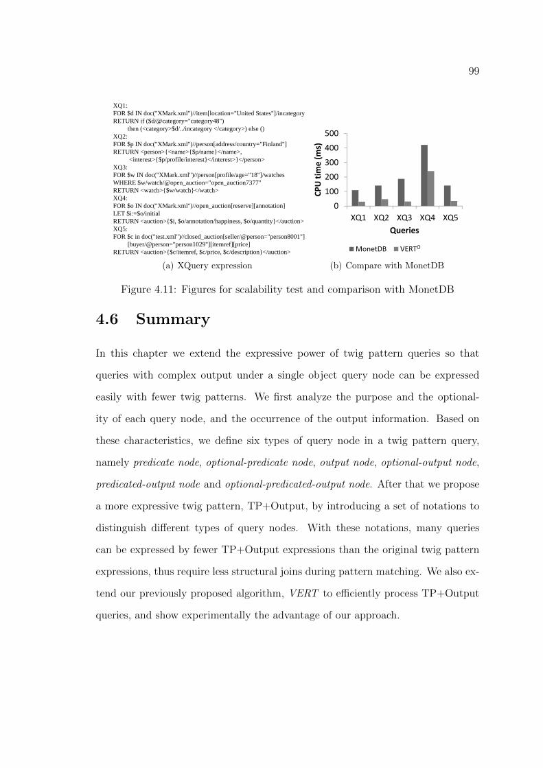
99





(a) XQuery expression







//altname 360 125 125 235

0

0


query

//item 984 328 328 656

//person 1735 766 766 969

//person 1360 532 532 828

//open_auction 3984 391 891 1093 2000

//closed_auction 1140 406 406 734

0


query

//article 1609 1484 1484 125

//inproceedings 4905 1468 1468 3437

//inproceedings 2437 1547 1547 890


//inproceedings 1734 1578 1578 156

0

scalability


0

1000

2000

3000

4000

5000

6000

DQ1 DQ2 DQ3 DQ4 DQ5

Execution tim

e (ms)

Queries

TP TP+Output

0

200

400

600

800

11.3 35.4 58.1 80

Execution tim

e (ms)

Data size (MB)

XQ1 XQ2 XQ3 XQ4 XQ5

0

100

200

300

400

500

XQ1 XQ2 XQ3 XQ4 XQ5

CPU tim

e (ms)

Queries

MonetDB VERTO

(b) Compare with MonetDB

Figure 4.11: Figures for scalability test and comparison with MonetDB

4.6 Summary

In this chapter we extend the expressive power of twig pattern queries so that

queries with complex output under a single object query node can be expressed

easily with fewer twig patterns. We first analyze the purpose and the optional-

ity of each query node, and the occurrence of the output information. Based on

these characteristics, we define six types of query node in a twig pattern query,

namely predicate node, optional-predicate node, output node, optional-output node,

predicated-output node and optional-predicated-output node. After that we propose

a more expressive twig pattern, TP+Output, by introducing a set of notations to

distinguish different types of query nodes. With these notations, many queries

can be expressed by fewer TP+Output expressions than the original twig pattern

expressions, thus require less structural joins during pattern matching. We also ex-

tend our previously proposed algorithm, VERT to efficiently process TP+Output

queries, and show experimentally the advantage of our approach.

100







//altname 360 125 125 235

0

0


query

//item 984 328 328 656

//person 1735 766 766 969

//person 1360 532 532 828

//open_auction 3984 391 891 1093 2000

//closed_auction 1140 406 406 734

0


query

//article 1609 1484 1484 125

//inproceedings 4905 1468 1468 3437

//inproceedings 2437 1547 1547 890


//inproceedings 1734 1578 1578 156

0

scalability


0

1000

2000

3000

4000

5000

6000

DQ1 DQ2 DQ3 DQ4 DQ5

Execution tim

e (ms)

Queries

TP TP+Output

0

200

400

600

800

1000

NQ1 NQ2 NQ3 NQ4 NQ5

Execution tim

e (ms)

Queries

DB2 VERTO

(a) NASA data







//altname 360 125 125 235

0

0


query

//item 984 328 328 656

//person 1735 766 766 969

//person 1360 532 532 828

//open_auction 3984 391 891 1093 2000

//closed_auction 1140 406 406 734

0


query

//article 1609 1484 1484 125

//inproceedings 4905 1468 1468 3437

//inproceedings 2437 1547 1547 890


//inproceedings 1734 1578 1578 156

0

scalability


Eti

ti(

)

0

500

1000

1500

2000

2500

3000

XQ1 XQ2 XQ3 XQ4 XQ5

Execution tim

e (ms)

Queries

DB2 VERTO

0

100

200

300

400

500

XQ1 XQ2 XQ3 XQ4 XQ5

CPU tim

e (ms)

Queries

MonetDB VERText

(b) XMark data







//altname 360 125 125 235

0

0


query

//item 984 328 328 656

//person 1735 766 766 969

//person 1360 532 532 828

//open_auction 3984 391 891 1093 2000

//closed_auction 1140 406 406 734

0


query

//article 1609 1484 1484 125

//inproceedings 4905 1468 1468 3437

//inproceedings 2437 1547 1547 890


//inproceedings 1734 1578 1578 156

0

scalability


0

1000

2000

3000

4000

5000

6000

DQ1 DQ2 DQ3 DQ4 DQ5

Execution tim

e (ms)

Queries

TP TP+Output

Execution tim

e (ms)

0

1000

2000

3000

4000

5000

Execution tim

e (ms) 0

2000

4000

6000

8000

10000

DQ1 DQ2 DQ3 DQ4 DQ5

Execution tim

e (ms)

Queries

DB2 VERTO

(c) DBLP data

Figure 4.12: Performance comparison between VERTO and DB2

101

CHAPTER 5

PERFORMING GROUPING AND

AGGREGATION IN XML QUERIES

Since more and more business data are represented in XML format, there is a

compelling need of supporting analytical operations in XML queries. Particularly,

the latest version of XQuery proposed by W3C, XQuery 1.1, introduces a new

construct to explicitly express grouping operation in FLWOR expression. Existing

works in XML query processing mainly focus on physically matching query struc-

ture to XML document. Given the explicit grouping operation in a query, how

to efficiently compute grouping and aggregate functions over XML document is

not well studied yet. In this chapter, we extend the VERT algorithm proposed in

Chapter 3, to efficiently perform grouping and aggregate function in XML queries.

We present experimental results to validate the efficiency of our approach, over

other existing approaches.

102

5.1 Introduction

As introduced in previous sections, existing works on XML query processing mainly

focus on how to efficiently match the query pattern to XML document, which is con-

sidered a core operation to process queries in most standard XML query languages.

As more and more business data are represented in XML format, analytical queries

involving grouping and aggregate operations have become more popular. To pro-

cess an analytical query with grouping, existing pattern matching techniques are

no longer effective. A new technique is required to handle the grouping operation

in queries.

Similar to relational databases, most analytical queries over XML documents

contain a main operator group-by and a set of aggregate functions such as max(

), min( ), sum( ), count( ), avg( ), etc. In most XML query languages, aggregate

functions are syntactically supported; however, the common shortcoming of many

XML query languages is the lack of explicit support for grouping. For example,

XQuery 1.0 is the widely adopted version of XQuery in most XQuery engines,

however, grouping in XQuery 1.0 can only be expressed implicitly using nesting.

This nested expression for representing the grouping operation can be neither well

understood and composed by users, nor easily detected by a query optimizer, as

pointed out by [10].

There are many efforts [14, 9, 72] on extending the expressive power for XQuery

to support grouping, until W3C publishes the latest version of XQuery, XQuery

1.1 [40], to introduce a new construct to explicitly express grouping in FLWOR

expressions. For example, consider the bookstore document shown in Fig. 5.1, and

a query to find the average book price for each publisher in each year. This query

can be expressed in XQuery 1.1 as follows:

103

bookstore(1:1000,1)

subject(2:63,2)

subject(64:321,2)

name(3:4,3)

“computer”

book(5:18,3)

title(8:9.4)

author(10:11,4)

publisher(6:7,4)

year(12:13,4)

price(14:15,4)

quantity(16:17,4)


book(19:34,3)

title(22:23.4)

author(24:25,4)

publisher(20:21,4)

year(28:29,4)

price(30:31,4)

quantity(32:33,4)

“Elco” “DatabaseSystems”

“Smith” 2005 32 20

book(35:48,3)

title(38:39.4)

author(40:41,4)

publisher(36:37,4)

year(42:43,4)

price(44:45,4)

quantity(46:47,4)

“Elco” “XML” “Smith” 2005 56 10

author(26:27,4)

Cole

…...

book(49:62,3)

title(52:53.4)

author(54:55,4)

publisher(50:51,4)

year(56:57,4)

price(58:59,4)

quantity(60:61,4)

“Elco” “DataReplication”

“Wang” 2006 60 25

Figure 5.1: An example document bookstore.xml

FOR $p IN distinct-values(doc(“bookstore.xml”)//book/publisher),

$y IN distinct-values(doc(“bookstore.xml”)//book/year),

LET $pr := doc(“bookstore.xml”)//book[publisher=$p and year=$y]/price

GROUP BY $p, $y

ORDER BY $p, $y

RETURN

<book publisher=“{$p}” year=“{$y}”>

<average price>{avg($pr)}</average price>

</book>

Although the work of XQuery 1.1 has just started, it reflects the importance of

grouping operations in XML queries. As a result, how to efficiently process XML

queries with grouping becomes a new research direction.

There are many relational approaches to process XML queries, as introduced in

Chapter 2. In these relational approaches, they normally shred XML documents

into tables and convert XML queries into SQL statements to query the database.

104

This sort of approaches can handle grouping in XML queries with the group-by

function in SQL. However, SQL has difficulty supporting multi-level (nested) group-

ing, which often appears in analytical XML queries. Also the primeval drawbacks

of relational approaches in query structural search are a big concern. A recent

work [50] proposed an algorithm to compute group-by queries natively over XML

document. They scan the document for each query and prune out irrelevant nodes.

For the relevant nodes, they merge and count the analytical attributes for each

group so that aggregate function can be easily performed. The major problem is

that their navigational approach is only suitable for queries with a simple pred-

icate. They find the relevant nodes in documents by scanning the document for

each query. However, if a query contains complex predicates as selection conditions

and the document schema is complex (e.g., “//”-axis query and documents with

recursively appearing tags), file scan is neither efficient, nor effective to return cor-

rect answers. That also explains why many twig pattern matching techniques, e.g.,

TwigStack [16], attract lots of research attention.

To solve the problem in structural search in existing work for XML query pro-

cessing with grouping, we extend our algorithm VERT proposed in Chapter 3, to

efficiently compute group-by operators in XML queries with complex predicates.

Given a group-by query, we match the query pattern to the document based on

query predicates using VERT. VERT can handle both structural search and con-

tent search in an XML query efficiently, thus it is suitable for queries with complex

predicates. After that, we use the table indexes to get the values of relevant prop-

erties and compute the aggregate functions in different levels of nested grouping by

scanning the resulting tuples.

The rest of this chapter is organized as follows. Related work on XML grouping

is presented in Section 5.2. In Section 5.3 and 5.4 we describe a format of queries

105

with grouping and aggregation, which is used in our system, and design the algo-

rithm VERTG to efficiently process queries. We present experimental results in

Section 5.5 and summarize this chapter in Section 5.6.

5.2 Related work on XML grouping

Grouping and aggregation is well supported by SQL in relational databases. There

are also research works [53, 73] to generalize or optimize such analytical operations

in RDBMS. Since XQuery 1.0 lacks functions to explicitly support grouping, pro-

cessing queries with grouping in XML is addressed by researchers in recent years.

Intuitively, the relational approaches to store and query XML data can support

grouping and aggregation because of the powerful SQL. However, these sort of

approaches have limitations in structural search, as reviewed in Chapter 2.

The research in XML grouping in native XML databases mainly focuses on three

directions. The first direction is on how to support grouping by either providing

logical grouping operators [43, 20, 96], or detecting grouping in nested queries and

rewriting queries [37, 42, 88, 101, 107]. Particularly, in [43] they provide algebraic

operators for grouping, and achieve efficient construction of XML elements using

their algebra. [20, 96] focus on designing a graphical query language supporting

grouping, and eventually the query will be translated to XQuery expression to

process. The works [37, 42, 88, 101, 107] detect the potential grouping from nested

queries and using different rewriting rules to transform the queries into a new

structure with explicit group-by operator. However, this approach has a bottleneck,

which is the difficulty of detecting grouping in nested queries. Sometimes it is even

not possible to detect such potential grouping [9].

Due to the limitation of detecting grouping in nested queries, some researchers

106

focus on a second direction, which is extending XQuery 1.0 to explicitly support

grouping in queries. In [14, 9, 72] they defined extra operator to complement

FLWOR expression in XQuery for grouping. In this case, the query optimizer does

not need to detect potential grouping in an XQuery expression. Based on these

research efforts, W3C published the new version of XQuery, XQuery 1.1 [40], in

which a grouping construct is introduced as a core requirement, though the work

has just started.

Since none of the works mentioned above focuses on physically computing group-

by and aggregate function over XML documents, a new research direction works

on algorithmic support for processing grouping and aggregation. [50] proposes an

algorithm to directly compute group-bys. However their method did not consider

the case that an XML query may contain complex predicate and the document may

also have a complex schema such as containing recursively appearing elements. For

such documents and queries, the file scan to select relevant nodes in [50] may fail to

work, and this motivates many pattern matching techniques ([52]). There are also

works ([89]) to eliminate duplicates during grouping computation so that better

performance can be retrieved.

5.3 Query expression

In this section, we describe the general form of XML queries with grouping, which

is used in our VERTG algorithm. The general query form is shown in Fig. 5.2.

The reason why we introduce this query form is that we want to separate the

query pattern from the grouping and aggregate functions. The main components

in our query form are:

Pattern: The grouping operation and aggregate function is built on twig pattern

107

Expr ::= “PATTERN:” XPath_expressionGroup by*

Group by ::= “GROUP BY:” group by_attribute+ (“ORDER BY:” group by_attribute+)? (“HAVING:” condition+ )? “RETURN: {” aggregate_function+ Group by* “}”

Occurrence Indicator: + 1 or more * 0 or more ? 0 or 1

Figure 5.2: Query form used by VERTG

queries because twig pattern is the core pattern for general XML queries. We use

XPath expressions to represent twig patterns. The nodes in a twig pattern should

include all the predicate nodes, group-by nodes and output nodes in the given

query1.

Grouping: Grouping is explicitly expressed in the group by clause. Group by in-

dicates the query nodes by which the results are grouped, and an optional order by

clause indicates the order to output each group. Without indicating the grouping

order, we will output the result based on the ascending order of the group-by nodes

by default. Grouping often comes with optional having clause, which is used to

specify the aggregate conditions. Grouping can be parallel, which means the results

are grouped in multiple ways by different properties. Grouping can also be nested,

which means the results within each return clause can be further grouped.

Return: The return clause specifies the aggregate functions in each group. As

mentioned above, grouping can recursively appear in a query, so the output infor-

mation following the return clause can be the value of an aggregate function, or a

nested grouping operation with another return clause.

1Note that, if the query pattern is complex, we will use multiple twig patterns with joins orthe TP+Output expression introduced in Chapter 4, to represent the query pattern. Details arediscussed in Section 5.4.6

108

Example 5.1. Consider a query to find first all the computer books grouped by

publisher to output the total number of books of each publisher whose average book

price is greater than 40, and then group all books under each of these publishers by

year and price separately to find the total quantity of books in each subgroup. This

query can be expressed as Q7 in Fig. 5.3. Note that the pattern in Q7 is an XPath

expression in which all relevant nodes to the query are included.

Q7: PATTERN: subject[name=”computer”]/book[publisher][year][price][quantity] GROUP BY: publisher ORDER BY: publisher HAVING: avg(price)>40 RETURN: { count(book), GROUP BY: year RETURN: { sum(quantity) } GROUP BY: price RETURN: { sum(quantity) } }

Figure 5.3: Example query Q7

5.4 VERTG algorithm

In this section, we introduce the algorithm VERTG to perform grouping as well

as aggregate functions in XML queries with complex predicate. Our algorithm

contains two phases. In the first phase, we perform pattern matching to find all

the relevant nodes that satisfy the query predicates in XML document. In our

implementation we use the algorithm VERT, which is presented in Chapter 3, to

match query pattern, because: (1) VERT solves content problems existing in many

other algorithms, such as the inefficiency of content management, content search

and content extraction, and (2) VERT makes use of relational tables to index

values, which is more compatible with the algorithm proposed in this chapter.

After that, in the second phase we use the table indexes on values, together with

109

the result from pattern matching, to perform grouping and compute aggregate

functions. Multi-level grouping can be efficiently supported in VERTG.

5.4.1 Data structures and output format

We define the query format in Section 5.3. In this section, we discuss how we

store document information and query information into relevant data structures,

which will be used during query processing with VERTG. Since we adopt VERT

to process pattern matching for queries, we need to maintain inverted lists and

relational tables, as mentioned in Chapter 3. We do not repeat the process to

construct these data structures. Take the document in Fig. 5.1 as an example, the

relational tables for the property title and author are shown in Fig. 5.4.

Label Value

Rtitle Label Value

(10:11,4) Green

Rauthor

(8:9,4) Network

(22:23,4) Database Systems

(38:39,4) XML

( , )

(24:25,4) Smith

(26:27,4) Cole

(40 41 4) S ith( , )

(52:53,4) Data Replication(40:41,4) Smith

(54:55,4) Wang

Figure 5.4: Relational tables for “title” and “author”

Besides the table indexes, we also need three tree structures for queries in

VERTG. The first one is a twig pattern, named TP, to represent the XPath

expression in a query. The second one is a grouping tree, named GT, to reflect the

structure of the complex grouping operations in a query. The last one is a skeleton

tree, named ST, to summarize the structural information of output. TP is used

to match to the document. This pattern matching process can be considered as a

selection based on predicates. In GT, each node stands for a grouping operation.

Thus within a GT node we record the group-by property2, the order-by property,

2To simplify the explanation, we assume there is one group-by property in each grouping

110

the grouping constraint and the output aggregate function. Each GT node has two

pointers: child and next sibling. The child points to a nested grouping operation,

and the next sibling points to a parallel grouping operation in the same grouping

level as the current node.

Example 5.2. Consider Q7 in Fig. 5.3. The structures TP, GT and ST for Q7

are shown in Fig. 5.5. In GT, the four entries in each node stand for group-

by property, order-by property, grouping constraint and output aggregate function

in order. The child pointer reflects the nested relationship between the two levels

of grouping, and the next sibling pointer reflects the parallel relationship between

the two grouping operations in the same level. ST is constructed based on GT. It

summarizes the structure of the output.

bookstore(1:1000,1)

subject(2:63,2)

subject(64:321,2)

name(3:4,3)

“computer”

book(5:18,3)

title(8:9.4)

author(10:11,4)

publisher(6:7,4)

year(12:13,4)

price(14:15,4)

quantity(16:17,4)


book(19:34,3)

title(22:23.4)

author(24:25,4)

publisher(20:21,4)

year(28:29,4)

price(30:31,4)

quantity(32:33,4)


“Smith” 2005 32 20

book(35:48,3)

title(38:39.4)

author(40:41,4)

publisher(36:37,4)

year(42:43,4)

price(44:45,4)

quantity(46:47,4)

“Elco” “XML” “Smith” 2005 56 10

author(26:27,4)

Cole

…...

book(49:62,3)

title(52:53.4)

author(54:55,4)

publisher(50:51,4)

year(56:57,4)

price(58:59,4)

quantity(60:61,4)


“Wang” 2006 60 25

Publisher_group

publisher no_of_book Year_group

year total_quantity

Price_group

price total_quantity

subject

name

“computer”

book

publisher year price quantity

GT:

child

next sibling

publisheravg(price)>40count(book)

publisher

yearyearnil

sum(quantity)

pricepricenil

sum(quantity)(a) TP

bookstore(1:1000,1)

subject(2:63,2)

subject(64:321,2)

name(3:4,3)

“computer”

book(5:18,3)

title(8:9.4)

author(10:11,4)

publisher(6:7,4)

year(12:13,4)

price(14:15,4)

quantity(16:17,4)


book(19:34,3)

title(22:23.4)

author(24:25,4)

publisher(20:21,4)

year(28:29,4)

price(30:31,4)

quantity(32:33,4)


“Smith” 2005 32 20

book(35:48,3)

title(38:39.4)

author(40:41,4)

publisher(36:37,4)

year(42:43,4)

price(44:45,4)

quantity(46:47,4)

“Elco” “XML” “Smith” 2005 56 10

author(26:27,4)

Cole

…...

book(49:62,3)

title(52:53.4)

author(54:55,4)

publisher(50:51,4)

year(56:57,4)

price(58:59,4)

quantity(60:61,4)


“Wang” 2006 60 25

Publisher_group


year total_quantity

Price_group


subject

name

“computer”

book

publisher year price quantity

TP:

child

next sibling

publisheravg(price)>40count(book)

publisher

yearyearnil

sum(quantity)

pricepricenil

sum(quantity)

(b) GT

bookstore(1:1000,1)

subject(2:63,2)

subject(64:321,2)

name(3:4,3)

“computer”

book(5:18,3)

title(8:9.4)

author(10:11,4)

publisher(6:7,4)

year(12:13,4)

price(14:15,4)

quantity(16:17,4)


book(19:34,3)

title(22:23.4)

author(24:25,4)

publisher(20:21,4)

year(28:29,4)

price(30:31,4)

quantity(32:33,4)


“Smith” 2005 32 20

book(35:48,3)

title(38:39.4)

author(40:41,4)

publisher(36:37,4)

year(42:43,4)

price(44:45,4)

quantity(46:47,4)

“Elco” “XML” “Smith” 2005 56 10

author(26:27,4)

Cole

…...

book(49:62,3)

title(52:53.4)

author(54:55,4)

publisher(50:51,4)

year(56:57,4)

price(58:59,4)

quantity(60:61,4)


“Wang” 2006 60 25

Publisher_group


year total_quantity

Price_group


(c) ST

Figure 5.5: Data structures for Q7: TP, GT and ST

operation. The data structures can be easily extended to support multiple group-by properties.The same assumption is made for grouping constraint and output aggregate function.

111

5.4.2 Query processing

To process a query with grouping using VERTG, we first perform a pattern match-

ing to the XML document. After that in the second phase we perform grouping

and aggregation based on the matching results.

Pattern matching:

As mentioned previously, we adopt VERT for pattern matching. At the beginning,

pattern matching returns tuples of labels for relevant matched nodes, which is

considered as intermediate result set, named as RSintermediate. The relevant nodes

means the nodes which are searched by the query, used as group-by properties, or

involved in aggregate functions. For example, to process Q7, we match the path

expression following PATTERN to the document. Since nodes “book”, “publisher”,

“year”, “price” and “quantity” appear in GROUP BY, HAVING and RETURN

clauses, pattern matching will output the labels for these nodes in each matched

segment. The intermediate result set for Q7 is shown in Fig. 5.6, where each tuple

contains the node labels in each twig pattern occurrence in document.

book publisher year price quantity

(5:18,3) (6:7,4) (12:13,4) (14:15,4) (16:17,4)

RSintermediate

(19:34,3) (20:21,4) (28:29,4) (30:31,4) (32:33,4)

(35:48,3) (36:37,4) (42:43,4) (44:45,4) (46:47,4)

(49:62 3) (50:51 4) (56:57 4) (58:59 4) (60:61 4)(49:62,3) (50:51,4) (56:57,4) (58:59,4) (60:61,4)

Figure 5.6: Pattern matching result for Q7

Performing grouping:

In the second phase, we perform grouping, as well as aggregate functions. We first

construct RSfinal by extracting actual values for the properties in the intermediate

112

result set RSintermediate using table indexes for each property. After that we traverse

the GT for the query according to a child-first fashion. The recursive method for

GT traversal is shown in Algorithm 5.1. We start with traverse (GT.root) and the

global variable level, which indicates the grouping level that we start performing

grouping with, is initialized to be 1. When we visit a node, we attach the group-by

property, order-by property, grouping constraint and aggregate function in that

node to the end of the corresponding global lists GL, OL, CL and AL. If a node

does not have a child, we begin to perform grouping in RSfinal with current GL,

OL, CL, AL and level. We also consider the parallel grouping within the same level

by checking the next sibling of each GT node. The level value is set to be the level

of the node which has a next sibling.

Algorithm 5.1 traverse (node)

1: attach the group-by property, order-by property, grouping constraint and ag-gregate function in node to the end of the lists GL, OL, CL and AL separately

2: if node.getChild == null then3: perform (RSfinal, GL, OL, CL, AL, level)4: else5: traverse (node.getChild)6: end if7: delete the last entry of GL, OL, CL and AL8: if node.getNextSibling != null then9: level=node.getLevel

10: traverse (node.getNextSibling)11: end if

To process the query Q7, we traverse the GT in Fig. 5.5(b). By Algorithm 5.1,

we perform grouping twice for Q7: one is for properties “publisher” and “year”

with level=1, and the other one is for “publisher” and “price” with level=2. Now

we move to the algorithm to perform grouping, which is shown in Algorithm 5.2.

Note that although the RSfinal is in relational table format, we cannot use SQL

to compute all the group-by clauses, because SQL cannot support nested grouping

113

due to the flat format of relational table.

We partition RSfinal in line 1. The function partition(RSfinal, GL,OL) sorts

the table RSfinal based on all the properties in GL, following the order by which

the properties appear in OL if it is different from that in GL. Sorting by multiple

properties works in the way that the system sorts tuples by the first property, and if

two or more tuples have the same value on the first property, then it sorts them by

the second property, and so forth. Now the tuples can be partitioned into different

groups for different levels.

Example 5.3. Consider Q7 in Fig. 5.3 with the intermediate result set shown in

Fig. 5.6. Using the index tables Rpublisher, Ryear, Rprice and Rquantity we can get the

exact values for each field. When the perform function is first called in Algorithm

5.1, we partition the RSfinal based on properties “publisher” and “year”. The result

is shown in Fig. 5.7. The bold lines in the RSfinal show the partition.

Level 1partition

Level 2partition

RS

publisher year book price quantity

Elco 2005 (19:34,3) 32 20

RSfinal

Elco 2005 (35:48,3) 56 10

Elco 2006 (49:62,3) 60 25

Hillman 2003 (5:18,3) 45 30( )

Figure 5.7: Example RSfinal with partition for Q7

In lines 2-6, we initialize the lists used in this algorithm. Particularly, cv[i] stores

the current value of the group-by property in the ith level group, while statistic lists

count[i][ ], sum[i][ ], max[i][ ] and min[i][ ] store the corresponding current statistic

values for the ith level group. In lines 7-31, we update these lists to get aggregate

results. We check each tuple in RSfinal to see whether any new partition in the

different levels begins at this tuple. This is done by checking whether the value

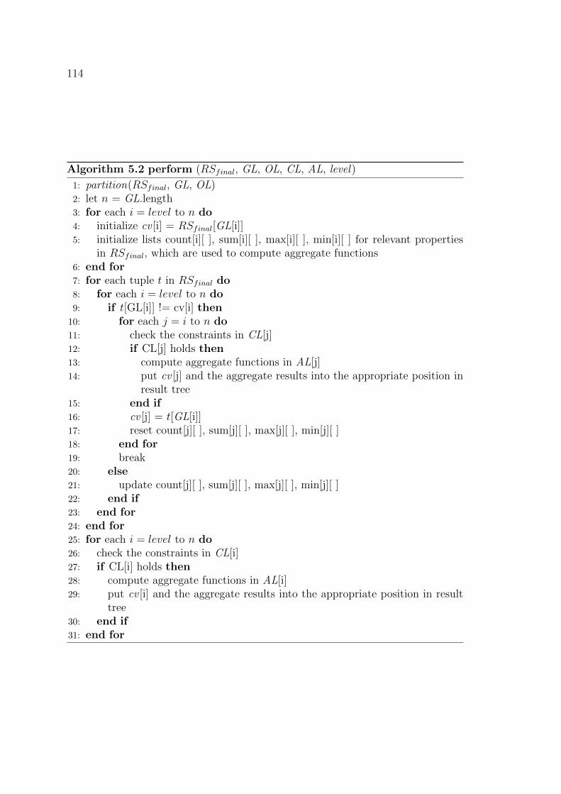
114

Algorithm 5.2 perform (RSfinal, GL, OL, CL, AL, level)

1: partition(RSfinal, GL, OL)2: let n = GL.length3: for each i = level to n do4: initialize cv [i] = RSfinal[GL[i]]5: initialize lists count[i][ ], sum[i][ ], max[i][ ], min[i][ ] for relevant properties

in RSfinal, which are used to compute aggregate functions6: end for7: for each tuple t in RSfinal do8: for each i = level to n do9: if t[GL[i]] != cv[i] then

10: for each j = i to n do11: check the constraints in CL[j]12: if CL[j] holds then13: compute aggregate functions in AL[j]14: put cv [j] and the aggregate results into the appropriate position in

result tree15: end if16: cv [j] = t[GL[i]]17: reset count[j][ ], sum[j][ ], max[j][ ], min[j][ ]18: end for19: break20: else21: update count[j][ ], sum[j][ ], max[j][ ], min[j][ ]22: end if23: end for24: end for25: for each i = level to n do26: check the constraints in CL[i]27: if CL[i] holds then28: compute aggregate functions in AL[i]29: put cv [i] and the aggregate results into the appropriate position in result

tree30: end if31: end for

115

of the group-by property in each level is changed in line 9. If any new partition

begins in a certain grouping level, for every lower level a new partition also begins.

Then we check the HAVING constraint in these levels and compute the aggregate

functions using the corresponding statistic lists, as shown in lines 11-15. After that

we reset the current group-by property value and the statistic lists for each of these

levels, in lines 16-17. If in a tuple, some grouping level does not end, we simply

update the statistic lists in line 21. In many cases, we do not need to maintain

all the statistic lists as the query may be only interested in some of them. To

simplify the presentation, we use all the statistic lists in the pseudo-code. Lines

25-31 finalize the query processing by outputting the result for the last group in

each grouping level.

Example 5.4. When the perform function is first called during GT traverse for

Q7, the RSfinal with partition is shown in Fig. 5.7. We start with level=1, and

initialize the current value and the necessary statistic lists for each grouping level,

as shown in Fig. 5.8. The list cv[ ] contains two entries since there are two levels

of grouping. The statistical list, saying count[1][ ], stores the total number of each

target property in the first level, e.g., count[1][2] is the count of the second property

“price” in level 1 grouping. Nil in some entries of each list means the corresponding

statistic value is not asked by the query and we do not need to maintain it.

cv[ ]publisher year

Elco 2005

count[1][ ] book price

0 0

sum[1][ ] 0

Note: In count[i][j] and sum[i][j], i is the grouping level and j is the position in the list.

quantity

sum[2][ ] 0

nil

nilnil

nil

nil

Figure 5.8: Example initial lists for Q7

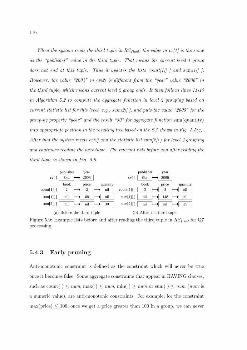
116

When the system reads the third tuple in RSfinal, the value in cv[1] is the same

as the “publisher” value in the third tuple. That means the current level 1 group

does not end at this tuple. Thus it updates the lists count[1][ ] and sum[1][ ].

However, the value “2005” in cv[2] is different from the “year” value “2006” in

the third tuple, which means current level 2 group ends. It then follows lines 11-15

in Algorithm 5.2 to compute the aggregate function in level 2 grouping based on

current statistic list for this level, e.g., sum[2][ ], and puts the value “2005” for the

group-by property “year” and the result “30” for aggregate function sum(quantity)

into appropriate position in the resulting tree based on the ST shown in Fig. 5.5(c).

After that the system resets cv[2] and the statistic list sum[2][ ] for level 2 grouping

and continues reading the next tuple. The relevant lists before and after reading the

third tuple is shown in Fig. 5.9.

cv[ ]publisher year

Elco 2005


2 2

sum[1][ ] 88

quantity

sum[2][ ] 30

nil

nil

nil

nilnil

(a) Before the third tuple

cv[ ]publisher year

Elco 2006


3 3

sum[1][ ] 148

quantity

sum[2][ ] 25

nil

nil

nil

nilnil

(b) After the third tuple

Figure 5.9: Example lists before and after reading the third tuple in RSfinal for Q7processing

5.4.3 Early pruning

Anti-monotonic constraint is defined as the constraint which will never be true

once it becomes false. Some aggregate constraints that appear in HAVING clauses,

such as count( ) ≤ num, max( ) ≤ num, min( ) ≥ num or sum( ) ≤ num (num is

a numeric value), are anti-monotonic constraints. For example, for the constraint

max(price) ≤ 100, once we get a price greater than 100 in a group, we can never

117

turn the constraint to be true, no matter how many more prices are checked in the

same group. Motivated by anti-monotonic constraints, some early pruning can be

done to enhance the query performance. When we read tuples in RSfinal, we can

check the anti-monotonic constraint first, rather than checking all constraints after

meeting the end tuple of the group. If any anti-monotonic constraint is violated by

a certain tuple, all other tuples in the same group can be skipped.

5.4.4 Extension flexibility

The query form and query processing algorithms presented in Section 5.3 and Sec-

tion 5.4.1 are built on basic aggregation. Sometimes the user may issue queries

involving keyword constraints distinct, or some other aggregate functions, or even

moving windows following the group-by properties. In this section, we explain

briefly how our algorithm is flexible to be extended to support these advanced

features.

Distinct:

Some aggregate function aims to find aggregate results on distinct values in a

group. In this case, we need to introduce keyword distinct. There are two types of

parameters that can be used by distinct constraint. The first type is property. For

example, count(distinct name) counts the number of different names distinguished

by name values. To support this type of distinct, we can maintain a sorted list to

store different values for the corresponding properties. When a value comes, we

can know whether it is a distinct value by checking the sorted list.

The second type of parameter following distinct constraint is object, e.g., count(

distinct book). This function is not easy to compute as “book” is an object class

rather than property, and there is no child value for “book” to explicitly distinguish

118

each “book” object. One way to distinguish objects under the same class is to

discover more semantics on object ID [18]. As long as the ID of an object class is

clear, we can easily perform aggregate functions on distinct objects by introducing

ID to RSfinal for the relevant object.

Other aggregate functions:

We discuss four more aggregate functions that are frequently asked, namely, maxN(

), minN( ), median( ) and mode( ). The function maxN( ) and minN( ) are top N

functions to find the N maximum or minimum values. Median( ) returns the value

that separates the higher half of a set of values from the lower half, and mode( )

is used to find the value that occurs most often in a set. In the discussion about

distinct keyword above, we mentioned that we can maintain an additional sorted

list to store different values for particular property. To compute maxN( ), minN(

), median( ) and mode( ), we not only need the sorted list for the distinct values

for relevant properties, but also need a frequency list in which each entry stores the

number of occurrences of the value in the corresponding entry in the sorted list.

Using these two lists, these aggregate functions can be easily computed.

Moving windows:

Moving windows are used to group answers by ranges of values on a certain prop-

erty. For example, a query needs to find the total quantity of books group by

range of 5 years with a moving step of 3 years, beginning at 2008. In this query,

we need to put books with year in [2008, 2012] together, with year in [2011, 2015]

together and so on. The general approach to handle moving windows is, we first do

grouping and aggregation as usual for each distinct value, and after that we per-

form a post-aggregation that aggregates the results from the previous step based

119

on each window range. Consider the query mentioned above. First we get the

sum(quantity) for each year, and then in the post-aggregation step, we just sum up

the quantity for years from 2008 to 2012, and from 2011 to 2015, etc. If there are

nested grouping operations inside each window group, the post-aggregation is also

effective. For example, continuing with the above query, suppose for each year win-

dow, we need to find the number of books grouped by publisher. In the first step,

we group books by each different year, and then in each group, we do a secondary

grouping on publisher and count the books in each subgroup. The post-aggregation

will integrate all subgroups in the five groups with year value from 2008 to 2012,

from 2011 to 2015, etc, by summing up the results under the same publisher.

5.4.5 Discussion on semantic optimization

In Q7, we group “book” by its own properties. Actually our algorithm also supports

grouping by the properties appearing in other places in document, rather than

descendant properties of a given object. Example 5.5 shows such a case.

Example 5.5. Consider the query Q8 to find the average price of books published

in 2005, group by publisher first and then group by subject name. In this query,

subject name appears as a property of another object, instead of “book”. To answer

this query, we just match the twig pattern shown in Fig. 5.10(a) to the document

tree, and extract values for each property using the table index for both “book” and

“subject”, to form RSfinal. Then grouping operation and aggregate functions can

be processed as normal in RSfinal. The result structure is shown in Fig. 5.10(b).

However, by investigating analytical queries, we find many of them group ob-

jects by their own properties. For example in Q7, we group books by publisher

and then by year and price. Publisher, year and price are all properties of book.

120

subject

name book

publisher priceyear

“2005”

(a) Twig pattern

Result

Publisher_group Publisher_group

pubisher Subject_group Subject_group

“Elco” name avg_price

……

……

name avg_price

“computer” “biology”49.3 64.5

(b) Result tree

Figure 5.10: Query Q8 and result tree

Naturally, we can adopt the semantic optimizations proposed in VERT in Chapter

3 to match query patterns to documents in VERTG.

We take the second optimization of VERT, which is using object tables to aid

twig pattern matching, to explain the advantages. The first advantage is the com-

plexity reduction of twig patterns during pattern matching with VERT. This is

illustrated in Section 3.3.2. The second advantage is when we generate RSfinal

from RSintermediate, we do not need to join with multiple property tables as in the

original VERT. Instead, we only need to join with one object table (and relevant

object/property tables for multi-valued properties, possibly), if the grouping prop-

erties are centered at one object. Thus, the performance can be improved. The

details of VERT optimizations are discussed in Chapter 3, so we do not repeat it

in this chapter.

5.4.6 Combining VERTO and VERTG

We proposed TP+Output expression to extend the existing twig pattern expression

to enhance the expressivity, and proposed VERTO to match a TP+Output pattern

query to an XML document, in Chapter 4. We discuss how to combine VERTO

and VERTG to serve queries with grouping and aggregation.

Actually VERTO and VERTG have different focuses for XML query process-

121

ing. VERTO focuses on the query structure, i.e., it models query predicates and

output information in a more expressive way, and match the query pattern to the

document. Whereas, VERTG focuses post-processing the pattern matching result

to support grouping and aggregation. In VERTG proposed in this chapter, we still

use the original twig pattern query to represent the structure of the a query involv-

ing grouping operations. If a query is complex in its output, we may need multiple

twig patterns to represent it. After matching all twig patterns to the document

and joining the results, we will post-process it for grouping and aggregation com-

putation. Since TP+Output expression proposed in Chapter 4 is used to model

complex query output, we can adopt TP+Output to represent the query pattern

in VERTG so that complex output nodes can be easily expressed in one or fewer

patterns. In this case, we will use VERTO to match the TP+Output query pat-

tern before performing grouping on the matching results, instead of using VERT

to match the original twig pattern as stated previously in this chapter.

Since VERTG emphasizes on its ability to perform grouping and aggregation,

for simplicity, we do not consider complex query pattern. Thus in this chapter we

still use VERT in illustrations.

5.5 Experiments

In this section we present experimental results. First we conduct experiments to

compare the performance of using VERT without optimization, with Optimization

1 and with Optimization 2 to perform pattern matching in VERTG. Consequently,

we name the three algorithms VERTG, VERTG-opt1 and VERTG-opt2. We show

that VERTG-opt2 has the best overall performance. Then we use VERTG-opt2

to compare with other approaches including an XQuery processor, MonetDB [13],

122

and a recently proposed algorithm N-GB [50] on group-by query processing.

5.5.1 Experimental settings

We implemented all algorithms in Java. The experiments were performed on a

dual-core 2.33GHz processor with 4G RAM. We still used the real-world data sets

DBLP (91MB) and NASA (23MB), and the well known synthetic data set XMark

in our experiments. The characteristics of the queries used is shown in Fig. 5.11.

Q G i G i Q G i G iQuery Groupinglevels

Groupingproperties

Query Groupinglevels

Groupingproperties

X1, N1, D1, XM1, NM1 1 1 XNR1, XNS1 1 2

2 2 2 2 2 2 S2 2X2, N2, D2, XM2, NM2 1 1 XNR2, XNS2 1 2

X3, N3, D3, XM3, NM3 1 2 XNR3, XNS3 2 3

X4, N4, D4, XM4, NM4 1 2 XNR4, XNS4 2 4

X5, N5, D5, XM5, NM5 2 3 XNR5, XNS5 3 5

X6, N6, D6, XM6, NM6 2 3 XNR6, XNS6 3 6

X7, N7, D7, XM7, NM7 2 4 DN1, DN2, DN3 1 1 2X7, N7, D7, XM7, NM7 2 4 DN1, DN2, DN3 1 1 2

X8, N8, D8, XM8, NM8 2 4 DN4, DN5, DN6 2 2 4

SX, SN, SD 1 6 1 6 DN7, DN8, DN9 3 3 6

Figure 5.11: Experimental queries with No. of grouping levels and No. of groupingproperties

5.5.2 Comparison between VERTG without and with opti-

mizations

Query performance

We process 8 queries in each document to compare the query performance between

VERTG and two optimizations, VERTG-opt1 and VERTG-opt2. Queries X1-X8

are issued to the XMark document, N1-N8 to the NASA document and D1-D8 to

the DBLP document. The experimental results on execution time are shown in

Fig. 5.12.

123

ibute

0

0

1 level 2 level 3 level 4 level 5 level 6 level

Number of grouping levels

Q1 Q2 Q3 Q4

1500

2000

2500on

time(m

s)

0

0

0

0

0

500

1000

X1 X2 X3 X4 X5 X6 X7 X8

Executio

Queries

VE VG

Q1 Q2 Q3 Q4 Q5 Q6 Q7 Q8 Q90

VERTG VERTG-opt1 VERTG-opt2

(a) XMark data set

ibute

0

0



Q1 Q2 Q3 Q4

3000

4000

5000

ontime(m

s)

0

0

0

0

0

1000

2000

N1 N2 N3 N4 N5 N6 N7 N8

Executio

Queries

VG VG 1 VG 2

Q1 Q2 Q3 Q4 Q5 Q6 Q7 Q8 Q90


(b) NASA data set

ibute

0

0



Q1 Q2 Q3 Q4400050006000700080009000

ontime(m

s)

0

0

0

0

01000200030004000

D1 D2 D3 D4 D5 D6 D7 D8

Executio

Queries

VG V 2

Q1 Q2 Q3 Q4 Q5 Q6 Q7 Q8 Q90


(c) DBLP data set

Figure 5.12: Query performance comparison for VERTG, VERTG-opt1 andVERTG-opt2

We can see that for all the queries VERTG-opt2 outperforms VERTG-opt1,

and VERTG-opt1 outperforms VERTG without optimization. This again validates

the analysis in Chapter 3 that using semantic optimizations can improve query

processing performance.

Scalability as grouping levels increase

It is natural that the user issues a query with nested grouping. In this section we

measure the time trend of VERTG and the optimizations when the grouping levels

increase. For each document, we select one type of query with predicates fixed and

124

grouping levels varied. The result on the scalability is shown in Fig. 5.13.

vels300004500 4000

5000

ontim

3500

5000

10000

15000

20000

25000

900

1800

2700

3600

Executiontime(m

s)

01000200030004000

D1 D2 D3 D4 D5 D6 D7 D8

Executio

Queries

VG VG 1 VG 2500

1000

1500

2000

2500

3000

Exection

time(m

s)

0

Q1 Q2 Q3 Q4 Q5 Q6 Q7 Q8 Q9

Queries

N GB VG VG opt

0



Q1 Q2 Q3 Q4

VGroup VGroup opt1 VGroup opt20




(a) XMark data with SX

vels300004500 4000

5000

ontim

3500

4000

5000

10000

15000

20000

25000

900

1800

2700

3600

Executiontime(m

s)

01000200030004000

D1 D2 D3 D4 D5 D6 D7 D8

Executio

Queries

VG VG 1 VG 2500

1000

1500

2000

2500

3000

3500

Exection

time(m

s)

0

Q1 Q2 Q3 Q4 Q5 Q6 Q7 Q8 Q9

Queries

N GB VG VG opt

0



Q1 Q2 Q3 Q4





(b) NASA data with SNvels300004500 4000

5000

ontim

1600018000

5000

10000

15000

20000

25000

900

1800

2700

3600

Executiontime(m

s)

01000200030004000

D1 D2 D3 D4 D5 D6 D7 D8

Executio

Queries

VG VG 1 VG 22000400060008000

10000120001400016000

Exection

time(m

s)

0

Q1 Q2 Q3 Q4 Q5 Q6 Q7 Q8 Q9

Queries

N GB VG VG opt

0



Q1 Q2 Q3 Q4





(c) DBLP data with SD

Figure 5.13: Scalability for VERTG, VERTG-opt1 and VERTG-opt2

From the result we can see that running time for VERTG increases as the

number of grouping levels increases. The reason is, if we group a set of objects

by a new property, we have to include that property for pattern matching, which

is time consuming. However, if we adopt VERTG with either VERTG-opt1 or

VERTG-opt2, we only match the relevant objects, instead of each property node.

As a result, the execution time increases slowly when more grouping levels are

involved. VERTG-opt2 is better than VERTG-opt1 because we access less tables

in VERTG-opt2.

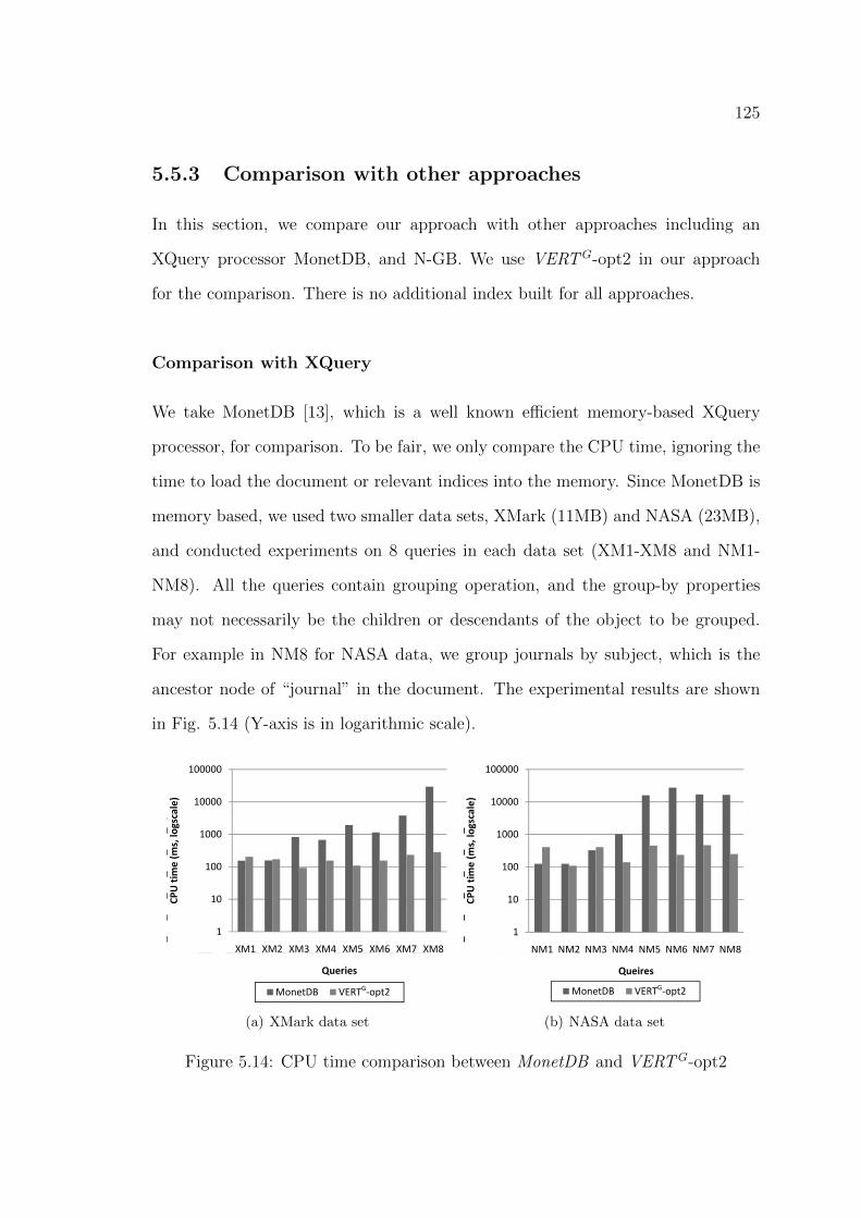
125

5.5.3 Comparison with other approaches

In this section, we compare our approach with other approaches including an

XQuery processor MonetDB, and N-GB. We use VERTG-opt2 in our approach

for the comparison. There is no additional index built for all approaches.

Comparison with XQuery

We take MonetDB [13], which is a well known efficient memory-based XQuery

processor, for comparison. To be fair, we only compare the CPU time, ignoring the

time to load the document or relevant indices into the memory. Since MonetDB is

memory based, we used two smaller data sets, XMark (11MB) and NASA (23MB),

and conducted experiments on 8 queries in each data set (XM1-XM8 and NM1-

NM8). All the queries contain grouping operation, and the group-by properties

may not necessarily be the children or descendants of the object to be grouped.

For example in NM8 for NASA data, we group journals by subject, which is the

ancestor node of “journal” in the document. The experimental results are shown

in Fig. 5.14 (Y-axis is in logarithmic scale).

e attribute

000 1000

10000

100000

,log

scale)

000

000

000

000

000

1

10

100

XM1 XM2 XM3 XM4 XM5 XM6 XM7 XM8

CPUtime(m

s

0

DN1 DN2 DN3 DN4 DN5 DN6 DN7 DN8 DN9

Queries

Queries

MonetDB VERTG-opt2

(a) XMark data set

e attribute

000 1000

10000

100000

,log

scale)

1000

10000

100000

,log

scale)

000

000

000

000

000

1

10

100

XM1 XM2 XM3 XM4 XM5 XM6 XM7 XM8

CPUtime(m

s

1

10

100

NM1 NM2 NM3 NM4 NM5 NM6 NM7 NM8

CPUtime(m

s

0


Queries

Queries

MonetDB Vp

Queires

MonetDB VERTG-opt2

(b) NASA data set

Figure 5.14: CPU time comparison between MonetDB and VERTG-opt2

126

For both data sets, we can see that for 1-level grouping with one property, Mon-

etDB performs well. However, when the number of group-by properties and the

number of grouping levels increases, since XQuery needs to express such queries

using nesting with multiple document retrievals and joins, the performance of Mon-

etDB is affected. In XMark data set, the CPU time for MonetDB increases fast on

XM3-XM8. In NASA data set, though the CPU time on NM3-NM4 is still relatively

low, when we increase the number of grouping levels in NM5-NM8, the efficiency

of MonetDB is significantly affected. Our approach, VERTG-opt2, outperforms

MonetDB for those queries with multi-level groupings.

Comparison with N-GB

We also compare our work with a recently proposed algorithm N-GB ([50]) to pro-

cess queries with grouping and aggregation. We take two larger data sets, XMark

(111MB) and DBLP (91MB) for the comparison. For XMark data, we perform

two sets of queries. The first set contains queries in which group-by properties

appear in any positional relationship with the object to be grouped. For example,

we group journals by either its child property “year” or its ancestor property “sub-

ject”. For this set of queries, our optimization can reduce the complexity during

query processing, but we still need pattern matching to get query node occurrences

in document. The second set of queries have group-by properties, output nodes

and aggregate properties under the same object. In this case, we do not need to

perform pattern matching, and the efficiency will be enhanced. For each query set,

we have 6 queries with grouping levels varying among 1, 2 and 3. Fig. 5.15 shows

the experimental results for XMark data.

From the figure above we can see VERTG-opt2 always outperforms N-GB. For

the first set of queries (Fig. 5.15(a)), VERTG-opt2 saves 30%-51% in running time,

127

one attributesels12000 1000

10000,log

scale)

1000

10000,log

scale)

5000

6000

7000e(m

s)

2000

4000

6000

8000

10000

1

10

100

XM1 XM2 XM3 XM4 XM5 XM6 XM7 XM

CPUtime(m

s

1

10

100

NM1 NM2 NM3 NM4 NM5 NM6 NM7 NM

CPUtime(m

s

0

1000

2000

3000

4000

Executiontime

0


Queries

Queries

MonetDB VERTG op2

Queires

MonetDB VERTG op2

XNR1 XNR2 XNR3 XNR4 XNR5 XNR6

Queries

N GB VERTG opt2

(a) Group-by properties in random position

one attributesels12000 1000

10000

,log

scale)

1000

10000

,log

scale)

5000

6000

7000

e(m

s)

5000

6000

7000

e(m

s)

2000

4000

6000

8000

10000

1

10

100

XM1 XM2 XM3 XM4 XM5 XM6 XM7 XM

CPUtime(m

s

1

10

100

NM1 NM2 NM3 NM4 NM5 NM6 NM7 NM

CPUtime(m

s

0

1000

2000

3000

4000

Executiontime

0

1000

2000

3000

4000

Executiontime

0


Queries

Queries

MonetDB VERTG op2

Queires

MonetDB VERTG op2

XNR1 XNR2 XNR3 XNR4 XNR5 XNR6

Queries

N GB VERTG opt2

XNS1 XNS2 XNS3 XNS4 XNS5 XNS6

Queries

N GB VERTG opt2

(b) Group-by properties in the same object asoutputs

Figure 5.15: Execution time comparison between N-GB and VERTG-opt2 forXMark data

and for the second query set (Fig. 5.15(b), this saving becomes 86%-93%.

We also used the real-world data DBLP to compare our approach and N-GB.

We used 9 queries for DBLP data, which are DN1-DN9. Since N-GB assumes

the answer tree can fit in memory, we allocated 1GB memory for JVM during

experiments. The results are shown in Fig. 5.16. We can see from the figure,

VERTG-opt2 outperforms N-GB for all kinds of queries. This result shows that

our approach is efficient not only for complex documents (e.g., XMark), but also

for flat documents (e.g., DBLP).

5.6 Summary

In this chapter we analyzed the drawbacks of different existing approaches to pro-

cess XML queries with grouping and aggregation, and proposed a novel algorithm,

VERTG, which can perform both parallel and nested grouping operations and

compute aggregate functions efficiently in XML queries with complex predicate.

VERTG extends the VERT algorithm which introduces table index during XML

128

e levels12000

2000

4000

6000

8000

10000

Executiontime(m

s)

0


Queries

N GB VERTG-opt2

Figure 5.16: Execution time comparison between N-GB and VERTG-opt2 forDBLP data

query processing. After matching the pattern of an XML query to the document

natively using VERT, VERTG extracts actual values for relevant nodes with ta-

ble indexes and then performs different levels of grouping and aggregation. Fur-

thermore, we can also adopt the semantic optimizations in VERT to significantly

enhance the query processing performance. We conducted experiments to com-

pare our approach with a well known XQuery processor, MonetDB and a recently

proposed algorithm, N-GB to show the advantages of our approach.

129

CHAPTER 6

CONCLUSION

6.1 Conclusion

In this thesis, we propose to use semantic information such as value, property,

object and relationship among objects, to improve the efficiency of XML query

processing. The core technique of our research is to integrate semantic relational

tables into native XML query processing approaches, which use inverted lists to

process twig pattern queries. With relational tables, for the first time, one can sep-

arately process content search to reduce the relevant inverted lists and the number

of structural joins for structural search, and thus improve search efficiency. Also

using relational tables one can effectively extract values based on node labels to

return to users. We theoretically and experimentally demonstrate that our seman-

tic approach can achieve better performance in twig pattern query processing than

existing approaches.

In Chapter 3, we propose the VERT algorithm to process XML twig pattern

130

queries. We first analyze the shortcomings in the structural join based native XML

twig pattern query processing approach, which is the state-of-the-art approach and

considered more efficient than other twig pattern query processing approaches in

general. In particular, the structural join based approach has difficulties in (1)

managing tremendous number of inverted lists for different values, (2) performing

content search for value predicates (e.g., range search price<50 ), and (3) extracting

values to answer a query. To solve these limitations, we introduce semantics-based

relational tables as an index to manage values in XML data. Using relational tables,

we can easily manage the tremendous number of data values in an XML document

as tuples. Also we can efficiently perform content search for query predicates and

return value answers to users. Especially to be mentioned is our relational tables

are constructed based on semantic information. Initially we use the default se-

mantics in XML documents, which is the parent node of each value must be its

associated property, to build property tables. A property table stores the label

of each document node that in this property type, and its corresponding value.

Content search in a query is performed by SQL selection in relevant property ta-

bles, and the selected property labels are used to construct new inverted lists for

the related property query nodes. After performing content search, the query can

be simplified by removing the value predicates to reduce the number of structural

joins, and the structural search can be performed by any existing efficient struc-

tural join algorithms, with the new inverted lists for related query nodes. Later we

use more semantics on relationship between object and property and relationship

among objects, to further optimize the relational tables to be object based. We

propose three optimizations which introduce object/property tables, object tables

and relationship tables respectively, to make twig pattern query processing more

efficient. Such semantic information is actually available in XML data, otherwise,

131

uses cannot compose, e.g., XQuery expressions to query XML data correctly. We

also show that our approach can be easily extended to process queries with ID

references and more general queries joining different twig patterns in one or several

documents.

Later, in Chapter 4 and 5 we extend twig pattern query to express complex

output information and to support grouping and aggregation respectively.

In Chapter 4, we explain the limitation of the existing twig pattern representa-

tion to express a subset of queries with complex output information centered at one

object. Normally such a query needs to be represented by multiple twig patterns

with joins to link them. Consequently, we have to match multiple twig patterns

and join the matching results. In our research, we analyze the characteristics of

query nodes, i.e., the purpose (predicate or output), the optionality (required or

optional) and the occurrence (one or many), and based on our analysis, we ex-

tend the existing twig pattern query to express complex output information, such

as optional output, predicated output and optional-predicated output. Using our

extension, which is named TP+Output, we can express the queries with complex

output information under a same object by fewer query patterns, compared to the

original twig pattern representation, and thus perform less structural joins to pro-

cess the query. Last, we extend the second optimization, which uses object tables,

of VERT to match TP+Output queries. We call the extended algorithm VERTO.

In Chapter 5 we present how we extend the VERT algorithm to perform group-

ing and aggregations (e.g., sum, avg, max, min, etc.) in XML queries, to meet the

compelling needs of analytical queries in business data. We model the query pat-

tern part and the grouping operation part in an XML query separately. Then our

extended algorithm, VERTG, adopts VERT to match the query pattern part to

document first, and then traverse the grouping tree, which is constructed to reflect

132

the complex grouping operations in the query, to perform grouping and compute

aggregate functions. Our approach can effectively link the efficient twig pattern

matching algorithms to grouping and aggregation computation, which is not well

studied in existing twig pattern query processing works. We also show that the

semantic optimizations in VERT and the extended algorithm VERTO can also be

used in VERTG to model and process query patterns, to achieve better overall

performance.

6.2 Future work

Our research opens a new direction to use semantic information and to integrate

the data structures and indexes for both structured data and unstructured data, to

improve query processing in semistructured XML data. We demonstrate how our

approach solves the problems in value management and content search and meets

some practical functions that are not supported in existing XML query processing

approaches. In this section, we discuss the future research directions following our

semantic approach.

Twig pattern query processing has attracted considerable research attention.

However, many queries cannot be expressed with a single twig pattern. We pro-

posed TP+Output to extend the expressivity of twig pattern query for complex

output information. Although TP+Output effectively represents queries with com-

plex output centered at a unique object by one enhanced twig pattern, it still cannot

model any complex query, probably expressed in XQuery, using a single twig. For

example, some queries require value-based joins to link multiple twigs and each of

them can be represented by a TP+Output expression. Thus one future research

direction is to translate a general XQuery expression into one or several join-linked

133

TP+Output expressions, so that our TP+Output and its corresponding query pro-

cessing algorithm can be used to process general queries.

Our work focuses on handling content search in twig pattern queries with basic

PC and AD edges. There are research works performing structural joins in twig

pattern queries with OR-predicate, NOT-predicate, wildcards, etc, as these predi-

cates may appear in general XPath and XQuery expressions. Thus how to extend

our algorithms to solve the queries with these predicates can be another future

research direction. Also though in our algorithms we can extract actual values to

answer a twig pattern query, the format of returned result is still in tuples. How to

correctly and efficiently transform tuple result into XML format to output to users

needs to be studied.

Last, this thesis focuses on using semantics, e.g., object information, to process

structured XML query. Actually, by noticing such semantics, we can also improve

the search quality and efficiency in XML keyword search. Some of our research

works studied how to utilize object-based semantics in XML keyword query pro-

cessing, e.g., [6]. More continuous work is required to achieve better search quality

and efficiency in XML keyword search.

BIBLIOGRAPHY

[1] S. Al-Khalifa, H. V. Jagadish, J. M. Patel, Y. Wu, N. Koudas, and D. Srivas-

tava. Structural joins: A primitive for efficient XML query pattern matching.

In ICDE, pages 141–152, 2002.

[2] A. Arion, V. Benzaken, I. Manolescu, and Y. Papakonstantinou. Structured

materialized views for XML queries. In VLDB, pages 87–98, 2007.

[3] A. Arion, V. Benzaken, I. Manolescu, Y. Papakonstantinou, and R. Vijay.

Algebra-based identification of tree patterns in XQuery. In Flexible Query

Answering Systems, pages 13–25, 2006.

[4] A. Balmin, F. Ozcan, K. S. Beyer, R. Cochrane, and H. Pirahesh. A frame-

work for using materialized XPath views in XML query processing. In VLDB,

pages 60–71, 2004.

[5] Z. Bao, J. Lu, T. W. Ling, L. Xu, and H. Wu. An effective object-level XML

keyword search. In DASFAA, pages 93–109, 2010.

134

135

[6] Z. Bao, J. Lu, T. W. Ling, L. Xu, and H. Wu. An effective object-level XML

keyword search. In DASFAA, pages 93–109, 2010.

[7] Z. Bao, H. Wu, B. Chen, and T. W. Ling. Using semantics in XML query

processing. In ICUIMC, pages 157–162, 2008.

[8] C. Barton, P. Charles, D. Goyal, M. Raghavachari, M. Fontoura, and V. Josi-

fovski. Streaming XPath processing with forward and backward axes. In

ICDE, pages 455–466, 2003.

[9] K. S. Beyer, D. D. Chamberlin, L. S. Colby, F. Ozcan, H. Pirahesh, and

Y. Xu. Extending XQuery for analytics. In SIGMOD Conference, pages

503–514, 2005.

[10] K. S. Beyer, R. Cochrane, L. S. Colby, F. Ozcan, and H. Pirahesh. XQuery

for analytics: Challenges and requirements. In XIME-P, pages 3–8, 2004.

[11] K. S. Beyer, R. Cochrane, V. Josifovski, J. Kleewein, G. Lapis, G. M. Lohman,

R. Lyle, F. Ozcan, H. Pirahesh, N. Seemann, T. C. Truong, B. Van der

Linden, B. Vickery, and C. Zhang. System RX: One part relational, one part

XML. In SIGMOD, pages 347–358, 2005.

[12] P. Bohannon, J. Freire, P. Roy, and J. Simeon. From XML schema to rela-

tions: A cost-based approach to XML storage. In ICDE, pages 64–75, 2002.

[13] P. A. Boncz, T. Grust, M. van Keulen, S. Manegold, J. Rittinger, and J. Teub-

ner. MonetDB/XQuery: a fast XQuery processor powered by a relational

engine. In SIGMOD, pages 479–490, 2006.

[14] V. R. Borkar and M. J. Carey. Extending XQuery for grouping, duplicate

elimination, and outer joins. In XML Conference and Expo., 2004.

136

[15] E. W. Brown, J. P. Callan, and W. B. Croft. Fast incremental indexing for

full-text information retrieval. In VLDB, pages 192–202, 1994.

[16] N. Bruno, N. Koudas, and D. Srivastava. Holistic twig joins: optimal XML

pattern matching. In SIGMOD, pages 310–321, 2002.

[17] P. Buneman, B. Choi, W. Fan, R. Hutchison, R. Mann, and S. Viglas. Vec-

torizing and querying large XML repositories. In ICDE, pages 261–272, 2005.

[18] P. Buneman, S. B. Davidson, W. Fan, C. S. Hara, and W. C. Tan. Keys for

XML. In WWW, pages 201–210, 2001.

[19] S. Buttcher, C. L. A. Clarke, and B. Lushman. Hybrid index maintenance

for growing text collections. In SIGIR, pages 356–363, 2006.

[20] S. Ceri, S. Comai, E. Damiani, P. Fraternali, S. Paraboschi, and L. Tanca.

XML-GL: a graphical language for querying and restructuring XML docu-

ments. In WWW, pages 1171–1187, 1999.

[21] C. Y. Chan, W. Fan, and Y. Zeng. Taming XPath queries by minimizing

wildcard steps. In VLDB, pages 156–167, 2004.

[22] A. B. Chaudhri, A. Rashid, and R. Zicari. XML data management: native

XML and XML-enabled database systems. Addison-Wesley, 2003.

[23] D. Chen and C. Chan. ViewJoin: Efficient view-based evaluation of tree

pattern queries. In ICDE, pages 816–827, 2010.

[24] L. Chen, A. Gupta, and M. E. Kurul. Stack-based algorithms for pattern

matching on DAGs. In VLDB, pages 493–504, 2005.

137

[25] S. Chen, H. Li, J. Tatemura, W. Hsiung, D. Agrawal, and K. S. Candan.

Twig2Stack: bottom-up processing of generalized-tree-pattern queries over

XML documents. In VLDB, pages 283–294, 2006.

[26] T. Chen, J. Lu, and T. W. Ling. On boosting holism in XML twig pattern

matching using structural indexing techniques. In SIGMOD, pages 455–466,

2005.

[27] Y. Chen, S. B. Davidson, C. Hara, and Y. Zheng. RRXS: redundancy reduc-

ing XML storage in relations. In VLDB, pages 189–200, 2003.

[28] Y. Chen, S. B. Davidson, and Y. Zheng. BLAS: an efficient XPath processing

system. In SIGMOD, pages 47–58, 2004.

[29] Y. Chen, S. B. Davidson, and Y. Zheng. An efficient XPath query processor

for XML streams. In ICDE, pages 79–90, 2006.

[30] Z. Chen, H. V. Jagadish, L. V. S. Lakshmanan, and S. Paparizos. From tree

patterns to generalized tree patterns: on efficient evaluation of XQuery. In

VLDB, pages 237–248, 2003.

[31] J. Cheng, Y. Ke, W. Ng, and A. Lu. Fg-index: towards verification-free query

processing on graph databases. In SIGMOD, pages 857–872, 2007.

[32] J. Cheng, J. X. Yu, B. Ding, P. S. Yu, and H. Wang. Fast graph pattern

matching. In ICDE, pages 913–922, 2008.

[33] S. Chien, Z. Vagena, D. Zhang, V. J. Tsotras, and C. Zaniolo. Efficient

structural joins on indexed XML documents. In VLDB, pages 263–274, 2002.

[34] IBM DB2. http://ibm.com/db2/xml/.

138

[35] DBLP. http://dblp.uni-trier.de/.

[36] A. Deutsch, M. F. Fernandez, and D. Suciu. Storing semistructured data

with STORED. In SIGMOD, pages 431–442, 1999.

[37] A. Deutsch, Y. Papakonstantinou, and Y. Xu. The NEXT logical framework

for XQuery. In VLDB, pages 168–179, 2004.

[38] P. F. Dietz. Maintaining order in a linked list. In 14th annual ACM sympo-

sium on Theory of computing, pages 122–127, 1982.

[39] A. Doan, R. Ramakrishnan, F. Chen, P. DeRose, Y. Lee, R. McCann,

M. Sayyadian, and W. Shen. Community information management. IEEE

Data Eng. Bull., 29(1):64–72, 2006.

[40] D. Engovatov. XML query (XQuery) 1.1 requirements. W3C Working Draft,

2007.

[41] V. Ercegovac, V. Josifovski, N. Li, M. R. Mediano, and E. J. Shekita. Sup-

porting sub-document updates and queries in an inverted index. In CIKM,

pages 659–668, 2008.

[42] L. Fegaras, D. Levine, S. Bose, and V. Chaluvadi. Query processing of

streamed XML data. In CIKM, pages 126–133, 2002.

[43] T. Fiebig, S. Helmer, C. Kanne, G. Moerkotte, J. Neumann, R. Schiele, and

T. Westmann. Anatomy of a native XML base management system. VLDB

J., 11(4):292–314, 2002.

[44] D. Florescu and D. Kossmann. Storing and querying XML data using an

RDMBS. IEEE Data Eng. Bull., 22(3):27–34, 1999.

139

[45] M. Fontoura, V. Josifovski, E. Shekita, and B. Yang. Optimizing cursor

movement in holistic twig joins. In CIKM, pages 784–791, 2005.

[46] C. Galindo-Legaria and A. Rosenthal. Outerjoin simplification and reordering

for query optimization. ACM Trans. Database Syst., 22(1):43–74, 1997.

[47] M. R. Garey and D. S. Johnson. Computers and intractability: a guide to the

theory of NP-completeness. W. H. Freeman, 1979.

[48] H. Georgiadis and V. Vassalos. Improving the efficiency of XPath execution

on relational systems. In EDBT, pages 570–587, 2006.

[49] H. Georgiadis and V. Vassalos. XPath on steroids: exploiting relational

engines for XPath performance. In SIGMOD, pages 317–328, 2007.

[50] C. Gokhale, Nitin Gupta, Pranav Kumar, Laks V. S. Lakshmanan, Ray-

mond T. Ng, and B. A. Prakash. Complex group-by queries for XML. In

ICDE, pages 646–655, 2007.

[51] R. Goldman and J. Widom. DataGuides: Enabling query formulation and

optimization in semistructured databases. In VLDB, pages 436–445, 1997.

[52] G. Gou and R. Chirkova. Efficiently querying large XML data repositories:

A survey. IEEE Trans. Knowl. Data Eng., 19(10):1381–1403, 2007.

[53] J. Gray, A. Bosworth, A. Layman, and H. Pirahesh. Data cube: A rela-

tional aggregation operator generalizing group-by, cross-tab, and sub-total.

In ICDE, pages 152–159, 1996.

[54] N. Grimsmo, T. A. Bjørklund, and M. L. Hetland. Fast optimal twig joins.

In VLDB, 2010.

140

[55] T. Grust. Accelerating XPath location steps. In SIGMOD, pages 109–120,

2002.

[56] T. Grust, M. van Keulen, and J. Teubner. Staircase join: teach a relational

DBMS to watch its (axis) steps. In VLDB, pages 524–535, 2003.

[57] T. Grust, M. van Keulen, and J. Teubner. Accelerating XPath evaluation in

any RDBMS. ACM Trans. Database Syst., 29:91–131, 2004.

[58] A. K. Gupta and D. Suciu. Stream processing of XPath queries with predi-

cates. In SIGMOD, pages 419–430, 2003.

[59] A. Halverson, J. Burger, L. Galanis, A. Kini, R. Krishnamurthy, A. N. Rao,

F. Tian, S. Viglas, Y. Wang, J. F. Naughton, and D. J. DeWitt. Mixed mode

XML query processing. In VLDB, pages 225–236, 2003.

[60] B. C. Hammerschmidt, M. Kempa, and V. Linnemann. A selective key-

oriented XML index for the index selection problem in XDBMS. In DEXA,

pages 273–284, 2004.

[61] H. He and A. K. Singh. Closure-tree: An index structure for graph queries.

In ICDE, page 38, 2006.

[62] H. V. Jagadish, S. Al-Khalifa, A. Chapman, L. V. S. Lakshmanan, A. Nier-

man, S. Paparizos, J. M. Patel, D. Srivastava, N. Wiwatwattana, Y. Wu, and

C. Yu. TIMBER: A native XML database. The VLDB Journal, 11(4):274–

291, 2002.

[63] H. V. Jagadish, L. V. S. Lakshmanan, D. Srivastava, and K. Thompson.

TAX: A tree algebra for XML. In 8th International Workshop on Database

Programming Languages, pages 149–164, 2002.

141

[64] H. Jiang, H. Lu, and W. Wang. Efficient processing of XML twig queries

with OR-predicates. In SIGMOD, pages 59–70, 2004.

[65] H. Jiang, H. Lu, W. Wang, and B. C. Ooi. XR-Tree: Indexing XML data for

efficient structural joins. In ICDE, pages 253–263, 2003.

[66] H. Jiang, W. Wang, H. Lu, and J. X. Yu. Holistic twig joins on indexed XML

documents. In VLDB, pages 273–284, 2003.

[67] Z. Jiang, C. Luo, W. Hou, Q. Zhu, and D. Che. Efficient processing of XML

twig pattern: A novel one-phase holistic solution. In DEXA, pages 87–97,

2007.

[68] V. Josifovski, M. Fontoura, and A. Barta. Querying XML streams. VLDB

J., 14(2):197–210, 2005.

[69] R. Kaushik, P. Bohannon, J. F. Naughton, and H. F. Korth. Covering indexes

for branching path queries. In SIGMOD, pages 133–144, 2002.

[70] R. Kaushik, R. Krishnamurthy, J. F. Naughton, and R. Ramakrishnan. On

the integration of structure indexes and inverted lists. In SIGMOD, pages

779–790, 2004.

[71] R. Kaushik, P. Shenoy, P. Bohannon, and E. Gudes. Exploiting local simi-

larity for indexing paths in graph-structured data. In ICDE, pages 129–140,

2002.

[72] M. H. Kay. Positional grouping in XQuery. In XIME-P, 2006.

[73] W. Kim. On optimizing an SQL-like nested query. ACM Trans. Database

Syst., 7(3):443–469, 1982.

142

[74] B. Kimelfeld and Y. Sagiv. Twig patterns: From XML trees to graphs. In

WebDB, 2006.

[75] R. Krishnamurthy, V. T. Chakaravarthy, R. Kaushik, and J. F. Naughton. Re-

cursive XML schemas, recursive XML queries, and relational storage: XML-

to-SQL query translation. In ICDE, pages 42–53, 2004.

[76] R. Krishnamurthy, R. Kaushik, and J. F. Naughton. XML-SQL query trans-

lation literature: The state of the art and open problems. In Xsym, pages

1–18, 2003.

[77] A. Kurt and M. Atay. An experimental study on query processing efficiency

of native-XML and XML-enabled database systems. In DNIS, pages 268–284,

2002.

[78] C. Li and T. W. Ling. QED: a novel quaternary encoding to completely avoid

re-labeling in XML updates. In CIKM, pages 501–508, 2005.

[79] J. Li and J. Wang. Fast matching of twig patterns. In DEXA, pages 523–536,

2008.

[80] T. W. Ling, M. L. Lee, and G. Dobbie. Semistructured database design (web

information systems engineering and Internet technologies series. Springer-

Verlag, 2004.

[81] Z. Liu and Y. Chen. Identifying meaningful return information for XML

keyword search. In SIGMOD, pages 329–340, 2007.

[82] Z. H. Liu, S. Chandrasekar, T. Baby, and H. J. Chang. Towards a physi-

cal XML independent XQuery/SQL/XML engine. PVLDB, 1(2):1356–1367,

2008.

143

[83] J. Lu, T. Chen, and T. W. Ling. Efficient processing of XML twig patterns

with parent child edges: a look-ahead approach. In CIKM, pages 533–542,

2004.

[84] J. Lu, T. W. Ling, Z. Bao, and C. Wang. Extended XML tree pattern

matching: theories and algorithms. IEEE Trans. Knowl. Data Eng., 2010.

[85] J. Lu, T. W. Ling, C. Y. Chan, and T. C. From region encoding to extended

Dewey: On efficient processing of XML twig pattern matching. In VLDB,

pages 193–204, 2005.

[86] B. Ludascher, P. Mukhopadhyay, and Y. Papakonstantinou. A transducer-

based XML query processor. In VLDB, pages 227–238, 2002.

[87] B. Mandhani and D. Suciu. Query caching and view selection for XML

databases. In VLDB, pages 469–480, 2005.

[88] N. May, S. Helmer, and G. Moerkotte. Strategies for query unnesting in XML

databases. ACM Trans. Database Syst., 31(3):968–1013, 2006.

[89] N. May and G. Moerkotte. Efficient XQuery evaluation of grouping conditions

with duplicate removals. In XSym, pages 62–76, 2007.

[90] J. McHugh, S. Abiteboul, R. Goldman, D.n Quass, and J. Widom. Lore:

A database management system for semistructured data. SIGMOD Record,

26(3):54–66, 1997.

[91] P. Michiels, G. A. Mihaila, and J. Simeon. Put a tree pattern in your algebra.

In ICDE, pages 246–255, 2007.

[92] T. Milo and D. Suciu. Index structures for path expressions. In ICDT, pages

277–295, 1999.

144

[93] J. Morgenthal and J. Evdemon. Eliminating redundancy in XML using

ID/IDREF. XML Journal, 1(4), 2000.

[94] NASA. http://www.cs.washington.edu/research/xmldatasets/data/nasa/nasa.xml.

[95] S. Navathe, S. Ceri, G. Wiederhold, and J. Dou. Vertical partitioning algo-

rithms for database design. ACM Trans. Database Syst., 9(4):680–710, 1984.

[96] W. Ni and T. W. Ling. GLASS: A graphical query language for semi-

structured data. In DASFAA, pages 363–370, 2003.

[97] University of Pennsylvania. The penn treebank project,

http://www.cis.upenn.edu/∼treebank/.

[98] D. Olteanu, H. Meuss, T. Furche, and F. Bry. XPath: Looking forward. In

EDBT 2002 Workshops, pages 109–127, 2002.

[99] P. O’Neil, E. O’Neil, S. Pal, I. Cseri, G. Schaller, and N. Westbury. ORD-

PATHs: insert-friendly XML node labels. In SIGMOD, pages 903–908, 2004.

[100] S. Pal, I. Cseri, O. Seeliger, G. Schaller, L. Giakoumakis, and V. Zolotov.

Indexing XML data stored in a relational database. In VLDB, pages 1146–

1157, 2004.

[101] S. Paparizos, S. Al-Khalifa, H. V. Jagadish, L. V. S. Lakshmanan, A. Nier-

man, D. Srivastava, and Y. Wu. Grouping in XML. In EDBT Workshops,

pages 128–147, 2002.

[102] S. Paparizos, Y. Wu, L. V. S. Lakshmanan, and H. V. Jagadish. Tree logical

classes for efficient evaluation of XQuery. In SIGMOD, pages 71–82, 2004.

[103] F. Peng and S. S. Chawathe. XPath queries on streaming data. In SIGMOD,

pages 431–442, 2003.

145

[104] L. Qin, J. X. Yu, and B. Ding. wigList : Make twig pattern matching fast.

In DASFAA, pages 850–862, 2007.

[105] P. Ramanan. Covering indexes for XML queries: Bisimulation - simulation

= negation. In VLDB, pages 165–176, 2003.

[106] P. Rao and B. Moon. PRIX: Indexing and querying XML using prufer se-

quences. In ICDE, pages 288–300, 2004.

[107] C. Re, J. Simeon, and M. F. Fernandez. A complete and efficient algebraic

compiler for XQuery. In ICDE, page 14, 2006.

[108] M. Rys. State-of-the-art XML support in RDBMS: Microsoft SQL Server’s

XML features. IEEE Data Eng. Bull., 24(2):3–11, 2001.

[109] M. Rys. XML and relational database management systems: inside Microsoft

SQL Server 2005. In SIGMOD, pages 958–962, 2005.

[110] SAX parser. http://www.saxproject.org.

[111] A. Serna, J. K. Gerrikagoitia, G. Gil, and T. Smithers. XML data optimum

management with DB: Native-XML (open-source) and XML-enabled (pro-

prietor). In International Conference on Internet Computing, pages 149–156,

2005.

[112] M. Shalem and Z. Bar-Yossef. The space complexity of processing XML twig

queries over indexed documents. In ICDE, pages 824–832, 2008.

[113] J. Shanmugasundaram, E. Shekita, J. Kiernan, R. Krishnamurthy, E. Viglas,

J. Naughton, and I. Tatarinov. A general technique for querying XML doc-

uments using a relational database system. SIGMOD Record, 30(3):20–26,

2001.

146

[114] J. Shanmugasundaram, K. Tufte, C. Zhang, G. He, D. J. DeWitt, and J. F.

Naughton. Relational databases for querying XML documents: Limitations

and opportunities. In VLDB, pages 302–314, 1999.

[115] D. Shasha, J. T. Wang, and R. Giugno. Algorithmics and applications of tree

and graph searching. In PODS, pages 39–52, 2002.

[116] A. Spink. A user-centered approach to evaluating human interaction with web

search engines: an exploratory study. Inf. Process. Manage., 38(3):401–426,

2002.

[117] Sybase. http://www.sybase.com/products/databasemanagement/sqlanywhere.

[118] N. Tang, J. X. Yu, M. T. Ozsu, and K. Wong. Hierarchical indexing approach

to support XPath queries. In ICDE, pages 1510–1512, 2008.

[119] N. Tang, J. Xu Yu, M. T. Ozsu, B. Choi, and K. Wong. Multiple materialized

view selection for XPath query rewriting. In ICDE, pages 873–882, 2008.

[120] R. Tang, H. Wu, S. Nobari, and S. Bressan. Edit distance between XML and

probabilistic XML documents. In DEXA, pages 448–456, 2011.

[121] I. Tatarinov, S. D. Viglas, K. Beyer, J. Shanmugasundaram, E. Shekita, and

C. Zhang. Storing and querying ordered XML using a relational database

system. In SIGMOD, pages 204–215, 2002.

[122] S. Tatikonda, S. Parthasarathy, and M. Goyder. LCS-TRIM: Dynamic pro-

gramming meets XML indexing and querying. In VLDB, pages 63–74, 2007.

[123] D. Theodoratos, T. Dalamagas, A.s Koufopoulos, and N. H. Gehani. Se-

mantic querying of tree-structured data sources using partially specified tree

patterns. In CIKM, pages 712–719, 2005.

147

[124] F. Tian, D. J. DeWitt, J. Chen, and C. Zhang. The design and performance

evaluation of alternative XML storage strategies. SIGMOD Record, 31(1):5–

10, 2002.

[125] A. Tomasic, H. Garcia-Molina, and K. A. Shoens. Incremental updates of

inverted lists for text document retrieval. In SIGMOD, pages 289–300, 1994.

[126] H. Tong, C. Faloutsos, B. Gallagher, and T. Eliassi-Rad. Fast best-effort

pattern matching in large attributed graphs. In KDD, pages 737–746, 2007.

[127] Z. Vagena, M. M. Moro, and V. J. Tsotras. Twig query processing over

graph-structured XML data. In WebDB, pages 43–48, 2004.

[128] W3C Consortium. XML path language XPath 2.0,

http://www.w3.org/TR/xpath20/. 2007.

[129] W3C Consortium. XQuery 1.0: An XML query language,

http://www.w3.org/TR/xquery/. 2007.

[130] W3C Consortium. XQuery and XPath full text 1.0,

http://www.w3.org/tr/xpath-full-text-10/. 2007.

[131] H. Wang, J. Li, J. Luo, and H. Gao. Hash-based subgraph query processing

method for graph-structured XML documents. PVLDB, 1(1):478–489, 2008.

[132] H. Wang, S. Park, W. Fan, and P. S. Yu. ViST: A dynamic index method for

querying XML data by tree structures. In SIGMOD, pages 110–121, 2003.

[133] W. Wang, H. Wang, H. Lu, H. Jiang, X. Lin, and J. Li. Efficient processing of

XML path queries using the disk-based F&B index. In VLDB, pages 145–156,

2005.

148

[134] D. W. Williams, J. Huan, and W. Wang. Graph database indexing using

structured graph decomposition. In ICDE, pages 976–985, 2007.

[135] R. K. Wong, F. Lam, and W. M. Shui. Querying and maintaining a compact

XML storage. In WWW, pages 1073–1082, 2007.

[136] H. Wu, T. W. Ling, Z. Bao, and L. Xu. Object-oriented XML keyword search.

In ER, 2011.

[137] H. Wu, T. W. Ling, and B. Chen. VERT: A semantic approach for content

search and content extraction in XML query processing. In ER, pages 534–

549, 2007.

[138] H. Wu, T. W. Ling, B. Chen, and L. Xu. TwigTable: using semantics in

XML twig pattern query processing. JoDS, 15:102–129, 2011.

[139] H. Wu, T. W. Ling, and G. Dobbie. TP+Output: Modeling complex output

information in XML twig pattern query. In XSym, pages 128–143, 2010.

[140] H. Wu, T. W. Ling, G. Dobbie, Z. Bao, and L. Xu. Reducing graph matching

to tree matching for XML queries with ID references. In DEXA (2), pages

391–406, 2010.

[141] H. Wu, T. W. Ling, L. Xu, and Z. Bao. Performing grouping and aggregate

functions in XML queries. In WWW, pages 1001–1010, 2009.

[142] H. Wu, T. W. Ling, and Y. Zeng. Processing general XML queries: when

structural join meets value-based join. In submission to DASFAA, 2012.

[143] H. Wu, H. Takeda, M. Hamasaki, T. W. Ling, and L. Xu. An adaptive

ontology-based approach to identify correlation between publications. In

WWW, 2011.

149

[144] Y. Wu, J. M. Patel, and H. V. Jagadish. Estimating answer sizes for XML

queries. In EDBT, pages 590–608, 2002.

[145] Y. Wu, J. M. Patel, and H. V. Jagadish. Structural join order selection for

XML query optimization. In ICDE, pages 443–454, 2003.

[146] XMark. An XML benchmark project. http://www.xml-benchmark.org.

[147] L. Xu, Z. Bao, and T. W. Ling. A dynamic labeling scheme using vectors.

In DEXA, pages 130–140, 2007.

[148] L. Xu, T. W. Ling, Z. Bao, and H. Wu. Efficient label encoding for range-

based dynamic XML labeling schemes. In DASFAA, pages 262–276, 2010.

[149] L. Xu, T. W. Ling, and H. Wu. Labeling dynamic XML documents: An

order-centric approach. TKDE, 2011.

[150] L. Xu, T. W. Ling, H. Wu, and Z. Bao. DDE: from Dewey to a fully dynamic

XML labeling scheme. In SIGMOD, pages 719–730, 2009.

[151] W. Xu and Z. M. Ozsoyoglu. Rewriting XPath queries using materialized

views. In VLDB, pages 121–132, 2005.

[152] X. Yan, P. S. Yu, and J. Han. Graph indexing: A frequent structure-based

approach. In SIGMOD., pages 335–346, 2004.

[153] M. Yoshikawa, T. Amagasa, T. Shimura, and S. Uemura. XRel: a path-

based approach to storage and retrieval of XML documents using relational

databases. ACM Trans. Internet Techn., 1(1):110–141, 2001.

[154] C. Yu and H. V. Jagadish. Efficient discovery of XML data redundancies. In

VLDB, pages 103–114, 2006.

150

[155] T. Yu, T. W. Ling, and J. Lu. TwigStackList¬: A holistic twig join algorithm

for twig query with not-predicates on XML data. In DASFAA, pages 249–263,

2006.

[156] C. Zhang, J. F. Naughton, D. J. DeWitt, Q. Luo, and G. M. Lohman. On

supporting containment queries in relational database management systems.

In SIGMOD, pages 425–436, 2001.

[157] N. Zhang, N. Agarwal, S. Chandrasekar, S. Idicula, V. Medi, S. Petride, and

B. Sthanikam. Binary XML storage and query processing in Oracle 11g.

PVLDB, 2(2):1354–1365, 2009.

[158] N. Zhang, V. Kacholia, and M. T. Ozsu. A succinct physical storage scheme

for efficient evaluation of path queries in XML. In ICDE, pages 54–65, 2004.

[159] S. Zhang, M. Hu, and J. Yang. TreePi: A novel graph indexing method. In

ICDE, pages 966–975, 2007.

[160] P. Zhao, J. X. Yu, and P. S. Yu. Graph indexing: Tree + delta >= graph.

In VLDB, pages 938–949, 2007.

[161] L. Zou, L. Chen, and M. T. Ozsu. DistanceJoin: Pattern match query in a

large graph database. PVLDB, 2(1):886–897, 2009.