Accepted Manuscript

Using neural networks and the Markov Chain approach for facies analysis andprediction from well logs in the Precipice Sandstone and Evergreen Formation, SuratBasin, Australia

Jianhua He, Andrew D. La Croix, Jiahao Wang, Wenlong Ding, J.R. Underschultz

PII: S0264-8172(18)30552-X

DOI: https://doi.org/10.1016/j.marpetgeo.2018.12.022

Reference: JMPG 3641

To appear in: Marine and Petroleum Geology

Received Date: 2 July 2018

Revised Date: 2 December 2018

Accepted Date: 10 December 2018

Please cite this article as: He, J., La Croix, A.D., Wang, J., Ding, W., Underschultz, J.R., Using neuralnetworks and the Markov Chain approach for facies analysis and prediction from well logs in thePrecipice Sandstone and Evergreen Formation, Surat Basin, Australia, Marine and Petroleum Geology(2019), doi: https://doi.org/10.1016/j.marpetgeo.2018.12.022.

This is a PDF file of an unedited manuscript that has been accepted for publication. As a service toour customers we are providing this early version of the manuscript. The manuscript will undergocopyediting, typesetting, and review of the resulting proof before it is published in its final form. Pleasenote that during the production process errors may be discovered which could affect the content, and alllegal disclaimers that apply to the journal pertain.

MANUSCRIP

T

ACCEPTED

ACCEPTED MANUSCRIPT

Using Neural Networks and the Markov Chain Approach for Facies Analysis and Prediction from Well Logs in the Precipice Sandstone and Evergreen Formation, Surat Basin, Australia

Jianhua He a,b,c＊＊＊＊, Andrew D. La Croixc, Jiahao Wangc,d, Wenlong Ding a,b, J.R. Underschultze

a. School of Energy Resources，China University of Geosciences，Beijing 100083，China

b. Key Laboratory of Marine Reservoir Evolution and Hydrocarbon Enrichment Mechanism，Ministry of

Education，China University of Geosciences，Beijing 100083，China

c. Energy Initiative, University of Queensland, Brisbane, Australia 4072

d. Faculty of Earth Resource, China University of Geosciences, Wuhan 430074, China

e. Centre for Coal Seam Gas, Brisbane, University of Queensland, Australia 4072

* Corresponding author.

E-mail address: hejianhuadizhi@163.com

Postal address: School of Energy Resources,

China University of Geosciences, Beijing 100083, China

Tel.: +86 10 82320629

Fax: +86 10 82326850

MANUSCRIP

T

ACCEPTED

ACCEPTED MANUSCRIPT

Abstract: Facies analysis is crucial for reservoir evaluation because the

distribution of facies has significant impact on reservoir properties. Artificial

Neural Networks (ANN) are a powerful way to use facies interpretations from

core to determine equivalent facies from wireline logs in uncored wells.

However, ANN do not incorporate information that relates to facies

successions. This has limited the ability to effectively use facies information

derived from logs alone in reservoir modelling, especially at the regional scale

where data is often sparse, clustered, or incomplete. In this study, based on

observations of 8 cored wells with a total thickness of ~2000 m, 20 core facies

were defined that range from 0.22 m to 11.56 m thick. Facies were based on

grain size, sedimentary structures, and ichnological characteristics; Each facies

corresponds to a distinct depositional sub- environment within the broader

context of a large nearshore to shallow marine system. It was essential that these

facies were incorporated into reservoir models to accurately map the

distribution of reservoir and seal geobodies for CO2 storage assessment in the

Surat Basin, Australia. However, core data are few and far between in the Surat

Basin. To use core-defined facies in the absence of core, six wireline log

parameters – gamma ray, density, sonic, neutron, photoelectric factor, and deep

resistivity were plotted in multidimensional space and examined using Linear

Discriminator Analysis. Combined with model recognition and Fisher

Canonical Discriminance, the 20 core facies were simplified into 10

representative wireline log facies (WLF) with unique petrophysical parameters.

MANUSCRIP

T

ACCEPTED

ACCEPTED MANUSCRIPT

We then used the Markov Chains Approach (MCA) to determine the

significance of vertical facies transitions, which supported the interpretation that

facies group into 5 distinct associations: (1) channel-levee complex; (2) lower

delta plain; (3) subaqueous delta; (4) shoreface and; (5) tidal flats and channels.

Based on the facies analysis and statistical classification, Multilayer Perceptron

Classifier, a type of neural network method was applied using a training set of

three cored wells that had all 6 wireline log data under the monitor of the facies

successions determined from the MCA. Results show that the accuracy of WLF

prediction ranges from 66% to 99% (ca. 83%). The accuracy of facies

recognition decreased step wise with a decreasing number of logs as input data,

such that when only gamma ray, density, deep resistivity, and sonic were used

to train neural networks the accuracy dropped to between 45- 98% (ca. 67%),

depending upon the facies. This was considered the lowest acceptable threshold

of accuracy for facies determination for input into reservoir models for carbon

capture and storage. The results of this study show that sedimentary facies can

be accurately predicted for uncored intervals in the Precipice Sandstone and

Evergreen Formation to improve facies mapping and static reservoir modelling.

Additionally, wireline log facies are helpful for interpreting Lower Jurassic

stratigraphy, depositional setting, and basin evolution in the Mesozoic of

Eastern Australia.

Keywords: Surat Basin; Precipice Sandstone; Evergreen Formation; Facies Analysis; Neural Networks; Markov Chain Analysis.

MANUSCRIP

T

ACCEPTED

ACCEPTED MANUSCRIPT

1. Introduction

The Lower Jurassic Precipice Sandstone and Evergreen Formation are an

important prospective reservoir and seal target for potential future carbon

capture and storage (CCS) in the Surat Basin (Bradshaw, 2010). The geological

context in terms of depositional environment is poorly constrained especially in

the basin centre because of the fact that the strata are not thought to be

hydrocarbon bearing and therefore data is sparse. However, the basin centre is

also where carbon storage potential is highest. Depositional interpretations and

facies analysis have not been examined in detail, and this hinders the predictive

accuracy of reservoir performance and sealing potential. The level of detail of

the interpretation of depositional-facies and facies associations in the Precipice-

Evergreen succession is in need of an overhaul, and this will help establish more

realistic reservoir models for carbon-geostorage-site evaluation (Hodgkinson,

2013). This is because the sedimentary fabric, as well as grain size of different

facies will influence the hydraulic behaviour of strata in dynamic reservoir

simulation of CO2 injection. Capturing this detail may reduce uncertainty in the

prediction of plume migration and sealing potential of the top seal.

Sedimentary facies analysis is used to classify and map sedimentary

bodies, each which formed under unique depositional conditions. Facies are

typically assigned based on their physical or paleontogical characteristics

(Middleton, 1978; Dalrymple, 2010). However, facies differ in their intrinsic

MANUSCRIP

T

ACCEPTED

ACCEPTED MANUSCRIPT

textures and rock properties and this can greatly affect hydraulic and

mechanical properties (Chang et al., 2000, 2002; Burton and Wood, 2013; La

Croix et al., 2013; Baniak, 2014; He et al., 2016; La Croix et al., 2017).

Identification of sedimentary facies is based on both qualitative and quantitative

parameters, including mineral composition, texture and fabric, stratification,

sedimentary structures, bioturbation, grain-size distribution, and can be applied

in outcrop or core (Borer and Harris, 1991; Dill et al., 2005; Khalifa, 2005; Qi

and Carr, 2006; Qing and Nimegeers, 2008). However, geological datasets are

commonly limited in breath (e.g. outcrop) or due to cost (e.g. core), and thus

establishing facies relationships with regional perspective with limited control

data is often a challenge. Therefore, facies distributions based on well log data

are highly sought after (Berteig et al., 1985; Li and Anderson, 2006; Dubois et

al., 2007), as they represent the most abundant and widespread dataset in

subsurface studies. The prediction of facies from conventional wireline logs has

the potential to extend observations from the core scale (centimetres to metres)

to the well scale (meters or tens of metres), and ultimately to the regional scale

(> kilometers), allowing facies to be mapped. Nonetheless, the process of

quantitatively determining facies from well logs is currently being refined such

that it can be applied in a variety of sedimentary basins and in deposits from

different depositional environments (Tang et al., 2011; Wang and Timothy,

2013).

MANUSCRIP

T

ACCEPTED

ACCEPTED MANUSCRIPT

High precision sedimentary facies prediction is absolutely essential to

build large-scale, geologically reasonable, static reservoir models. Past studies

have focused on using statistical methods to analysze facies from well logs such

as discriminant analysis (Sakurai and Melvin, 1988; Avseth et al., 2001; Tang et

al., 2004), naïve Bayes classifier (Li and Anderson, 2006; He et al., 2016),

fuzzy logic (Cuddy, 2000; Saggaf and Nebrija, 2003), and support vector

machines (EI-Sebakhy et al., 2010; Wang et al., 2014; Deng et al., 2017). The

past decade has also seen successful application of Artificial Neural Networks

(ANN) (Derek et al., 1990; Wong et al., 1995; Siripitayananon et al., 2001;

Bhatt and Helle, 2002; Wang and Timothy, 2012) in the prediction of sandstone

and carbonate lithofacies because of the ability to unravel non-linear

relationships, quantify learning from training data, and work in conjunction with

other kinds of artificial intelligence (Bohling and Dubois 2003; Kordon 2010).

Multilayer perceptron classifier (MLPC) is a classifier based on feedforward

ANNs. MLPC is not a unique classifier for pattern recognition; however, the

merits of MLPC result in its broad application within various scientific and

academic fields (Micheli- Tzanakou 2000). MLPC is very flexible in the design

of learning algorithms, determining network architecture, selecting sensitive

input variables, and adapting codes for special issues (Wang and Carr, 2012b,

c). MLPC is a useful research tool because of its ability to solve complex

nonlinear problems stochastically, especially in shale lithofacies application

(Wang and Carr, 2012, 2013).

MANUSCRIP

T

ACCEPTED

ACCEPTED MANUSCRIPT

Most previous facies from wireline logs methods have determined facies at

each data point in the well, but failed to account for vertical continuity in the

facies profile (Lindberg and Grana, 2015). Each sample in the well log was

recognized independently from the adjacent samples. Therefore, unrealistic

facies successions tend to occur in facies profiles determined this way. Markov

Chain Analysis (MCA) has long been applied to determine whether the

occurrence facies in a stratigraphic succession are dependent on the underlying

facies (Gingerich, 1969; Le Roux, 1994; Xu and Maccarthy, 1998; Bohling and

Dubois, 2003). MCA results reveal the presence of preferred vertical

occurrences of facies in a sedimentary succession and therefore, can serve as

independent evidence to support interpretations of facies associations (Miall,

1973; Powers and Easterling, 1982; Wells et al., 1989; Carle et al., 1999). This

improves facies associations and facies succession prediction in complex and

variable sedimentary systems (Weissmann, 2005). To use the most effective and

reliable facies prediction method and include information about the vertical

relationships between facies, MCA are applied in this study.

The main objectives of this paper are to (1) use detailed interpretations of

the sedimentary-facies and facies classification to identify electrofacies from

conventional well logs and relate these to facies observed in core; (2) apply

statistical methods to predict and analyse electrofacies based on MLPC and

MCA; and, (3) use the electrofacies and electrofacies associations to map the

MANUSCRIP

T

ACCEPTED

ACCEPTED MANUSCRIPT

distribution of sedimentary environments in a small case-study area to provide

guidance for carbon capture and storage.

2. Geological setting

The Surat Basin is a large Early Jurassic to Early Cretaceous intra-cratonic

basin in eastern Australia and covers some 327, 000 km2 of Queensland and

New South Wales, Australia, from latitudes 25° -33° S, and from longitudes

147° to 152° E (Fig. 1A). The basin is filled with ~2500 m of clastic

sedimentary rocks and coal. The Eromanga and Clarence-Moreton basins (Fig.

1) are broadly time equivalent to the Surat Basin, connected on the western and

southeastern parts of the basin, respectively (Power and Devine, 1970; Exon,

1976; Green et al., 1997).

The Surat Basin developed as a shallow platform depression following 30

Ma of uplift, exposure, and non-deposition that eroded the top of the Bowen and

Gunnedah basins (Exon, 1976; Green et al., 1997). The major stages of basin

development and driving processes are not well studied, however, thermal

subsidence (Korsch et al., 1989), dynamic platform tilting (Gallagher et al.,

1994; Korsch and Totterdell, 2009; Waschbusch et al., 2009), and intraplate

rifting (Fielding, 1996) have been suggested as possible mechanisms. The Surat

Basin has several important structural features, the most important of which is

the Mimosa Syncline that forms the north-south axis of the basin (Fig. 1; Exon,

MANUSCRIP

T

ACCEPTED

ACCEPTED MANUSCRIPT

1976; Fielding et al., 1990; Hoffmann et al., 2009; Fielding et al., 1990; Raza et

al., 2009).

The Surat Basin was filled with sediment in six major fining upward pulses

/ cycles (Exon and Burger, 1981). The first cycle encompasses the Precipice

Sandstone and Evergreen Formation (Fig. 2). The Precipice Sandstone

represents braided river deposits characterized by thick cross-bedding with only

a few thin muddy intervals that lack marine palynoflora (Sell et al., 1972; Exon,

1976; Exon and Burger, 1981; Martin, 1981). However recent evidence has

shown that the deposition of the Lower Precipice Sandstone also could be

influenced by marine processes due to flaser and wavy bedding, clay drapes,

rare marine trace fossils and ‘brackish’ palynomorphs (Martin et al., 2018). In

contrast, the Evergreen Formation has been interpreted to represent deposits laid

down in meandering rivers and freshwater lakes. Though the upper parts of the

Evergreen Formation, including the Westgrove Ironstone Member and the

Boxvale Sandstone Member, show possible indications of marine influence on

deposition (Mollan et al., 1972; Exon, 1976). The Precipice Sandstone has a

maximum thickness of ~ 150 m and dominantly consists of quartzose, fine- to

coarse-grained sandstone with common siltstone and shale laminae in the upper

part (Exon, 1976). The finer-grained Evergreen Formation can be as thick as

300 m in addition to being geographically more widespread than the Precipice

Sandstone. The unit is dominated by carbonaceous siltstone with some horizons

of sandstone, carbonaceous mudstone, oolitic ironstone, and coal (Green et al.,

MANUSCRIP

T

ACCEPTED

ACCEPTED MANUSCRIPT

1997). This study will help elucidate the palaeoenvironments recorded by the

Precipice Sandstone and Evergreen Formation, because at present these remain

poorly constrained in a regional context.

The study area is located in the northern part of the Surat Basin. It covers

more than 21, 000 km2 (Fig. 1). 2D seismic data coverage across most of study

area helps constrain the lateral distribution of the Precipice Sandstone beyond

well control. A total of 192 wells across the basin had stratigraphic tops picked

based on well log signatures tied to core. Additionally, there are 8 cored wells

located within or in close proximity to the study area. Therefore, the study area

is an ideal case-study in which to test our facies prediction and mapping

capabilities. We chose two important intervals within the study area to

showcase the prediction and mapping of facies from logs. These are the

lowstand systems tract- LST which is defined by the sequence stractigraphic

surface ‘J10’ and ‘TS1’, and the overlying transgressive surface defined by the

surface ‘TS1’ and ‘MFS1’ (Wang et al., 2018). These represent the main

reservoir intervals being investigated for CCS, and the overlying seal.

3. Data Set and Methods

3.1 Database

This study utilizes sedimentological and ichnological core observations in

addition to wireline log data. The cumulative cored section that this study is

based on is approximately 2000 m from 8 wells (Fig. 1C). Core facies were

MANUSCRIP

T

ACCEPTED

ACCEPTED MANUSCRIPT

defined based on their sedimentological and ichnological characteristics,

including grain size, the nature of bedding contacts, physical structures,

biogenic structures, bioturbation intensity and the distribution of burrowing.

Wireline logs that were used for facies identification and prediction included

gamma ray (GR), bulk density (DEN), compressional slowness (SONIC), deep

resistivity (LLD), neutron porosity (NEUTRON), and photoelectric factor

(PDPE) from 31 wells. The logs have a resolution of 0.15 m.

Dataset selection and calibration are important for obtaining successful

facies identification and prediction results. Several quality-assurance steps were

performed on wireline logs to improve the outputs including depth correction,

normalization, and the removal of outliers. Outliers were defined using the

following criteria (Wong et al., 1998; Tang et al., 2011): (1) Intervals with null

or missing values (core missing); (2) Intervals with obvious post-depositional

overprints (fractures observed in core or image logs; hot sandstone influenced

by hydrothermal fluids input); (3) Intervals characterized by caliper-indicated

washouts or bad-wellbore conditions; (4) Intervals with facies thickness less

than 1.0 m; (5) An interval surrounding the contact between different logging

facies to remove the “averaging” of properties between two adjacent facies.

After establishing a robust and representative training set, neural-network

training can be conducted on the key core wells.

3.2 Discriminant and Principal Component Analysis

MANUSCRIP

T

ACCEPTED

ACCEPTED MANUSCRIPT

To develop a more accurate facies prediction model, pre-processing of the

training dataset was undertaken to identify a representative set of wireline

logging facies (WLF) from the set of core facies (CF). The representative input

database is the most important factor for controlling the quality of classifiers,

because successful application of neural networks generally requires clear

petrophysical and geological classification (Wong et al., 1998).

Linear discriminant analysis (LDA) and principal component analysis

(PCA) are two methods we used to extract and determine the main components

of variation within our dataset. These improve the accuracy of classifiers by

removing non-distinctive and interrelated features (Jungmann et al. 2011). LDA

is a multivariate method for finding a linear combination of features that

characterizes or separates two or more classes of samples (i.e., grouping

samples into major categories). Fisher canonical discriminant (FCD) is a

slightly different discriminant method from LDA that does not make some of

the assumptions that LDA does, such as normally distributed classes or equal

class covariance. FCD was used to double check the CF classification results by

LDA. PCA was used to determine the sensitivity of different types of well logs

to WLFs and also to determine the contribution of each log type to facies

differentiation. All types of CF could not be identified using conventional well

logs alone because core scale observations of structure and texture do not

necessarily translate to petrophysical properties. Therefore, LDA, PCA, and

MANUSCRIP

T

ACCEPTED

ACCEPTED MANUSCRIPT

FCD methods were all applied in this study to collectively achieve a useful set

of WLF to be predicted in wells lacking core.

3.3 The Markov Chain Analysis

The Markov Chain Analysis (MCA) is a statistical means of determining

the probability of transition between two states that are not controlled by the

previous state – i.e., they are “memoryless” (Grinstead and Snell. 1997). The

transition probability (Markov Chain) method is a modified form of indicator

kriging. In geological application, the method assumes the type of sediment that

will be deposited in a stratigraphic succession depends solely upon what is

currently being deposited in the present environment and not on the rock types

deposited in past environments (Jones et al., 2002). For example, in a

prograding shoreface environment, a gradual upward-coarsening succession of

facies will occur if no significant depositional hiatus exists (Fig. 3). In terms of

a vertical facies distribution, the probability of the occurrence of one facies is

dependent on the nearest occurrence of another facies over a lag interval. The

Markov chain can be mathematically described as follows: There is a set of

facies, F = {F1, F2, … , Fr}, which pass sequentially from one to another in

succession. Let the indicator variable, Ij(x), for facies j be defined as Ij(x) = {1,

if j occurs at x; 0, otherwise}, where x is a location in one vertical facies

succession. In terms of indicator variables, the marginal (initial) probability, Pj,

can be defined by

pj=E{I j(x)} (Equation 1)

MANUSCRIP

T

ACCEPTED

ACCEPTED MANUSCRIPT

The joint probability, pjk(h), can be also define by

pjk(h)=E{I j(x)Ik(x+h)} (Equation 2)

where h represents the lag distance in one direction (Fig. 3).

Fundamentally, the joint probability is the purest bivariate measure of spatial

variability. However, the transition probability of facies 1 passing into facies 2,

tjk(h) is the most interpretable, defined here with respect to indicator variables as

tjk(h)=E{I j(x)Ik(x+h)}/E{I j(x)} (Equation 3)

It can also be defined in terms of a conditional probability as

tjk(h)=Pr(k at x+h | j at x} (Equation 4)

Probability law requires that the row sums of the transition probability

matrix,T(h), sum to one and that the column sums obey

∑j pjtjk(h)= pk (Equation 5)

In this study, the probability of each facies transitioning to another was

calculated using PAleontological Statistics Software (PAST Version 3.17;

Hammer, 1999). Vertical facies succession analysis used an interactive

algorithm for Embedded Markov Chains (EMC) (Davis, 1986) based on the

PAST platform. The algorithm calculates a transition count matrix, a transition

probability matrix, an independent trials probability matrix, and a difference

matrix. In the transition probability matrix, the self-transition curves start at a

probability of 1 (100%) and decrease with increasing lag distances, whereas the

off-diagonal curves start at a probability of 0.0 (0%) and increase with lag

distance (Fig. 3; Carle, 1999). In the difference matrix, high positive entries

MANUSCRIP

T

ACCEPTED

ACCEPTED MANUSCRIPT

serve to emphasize the Markov property by suggesting which transitions have

occurred with greater than random frequency. The Powers-Easterling method in

this paper was used to test the matrix as a whole for non-randomness. It

determines the significance level of each facies transition and produces

preferred facies trends. The Powers-Easterling method yields the chi-square

value, degrees of freedom and critical value (Powers and Easterling, 1982).

3.4 Multi-Layer Perceptron Classifiers

We used a Multi-Layer Perceptron Classifier (MLPC), a form of

feedforward ANN (Haykin, 1998), to take the conventional wireline log input

data and determine the most probable WLF. MLPC consists of multiple layers

of nodes. Each layer is fully connected to the next layer in the neural network.

Nodes in the input layer represent input data; in this case wireline log data

consisting of DEN, SONIC, LLD, GR, NEUTRON, and PDPE. All other nodes

map inputs to outputs by a linear combination of the inputs with the node’s

weights w and bias b and applying an activation function (Fig. 4). This can be

written in matrix form for the MLPC with k + 1 layers as follows:

y(x) = fk (…f2 (w2Tf1 (w1

Tx + b1) + b2)…+ bK) (Equation 6)

Nodes in recurrent layers use sigmoid (logistic) function:

izi eZf −+

=1

1)(

(Equation 7)

Nodes in the output layer use softmax function:

MANUSCRIP

T

ACCEPTED

ACCEPTED MANUSCRIPT

∑ =

= N

k

z

z

ik

i

e

ezf

1

)(

(Equation 8)

The recurrent layer included two parts. The first was the computed distance

from the input vector to the training vector. The second layer summed these

contributions for each class of inputs to produce a vector probability. The

number of nodes N in the output layer corresponds to the number of classes; in

this case the 10 different types of wireline logging facies. The MCA helped us

understand the relationship between different logging facies and helped limit the

probability of a facies determinations that were not supported by the transition

probability analysis.

3.5 Neural Network Performance Evaluation and Application

We cross-validated our neural network results to determine the degree to

which outcomes were consistent and reliable. This was done by withholding

wireline log data from the control set, log by log, and then assessing the ratio of

times that the neural network made correct facies predictions as determined by

core facies in the training set. In addition, to decrease uncertainty in our results,

a convergence error was calculated to test the accuracy of facies prediction by

MLPC (Eyi, 2012). The convergence error (ɛc) is defined as follows:

ɛc = t

1KMAX

1k

t

tε

KMAX

1ε

= ∑=

， ( )KMAX1 ε,...,εmaxε = (Equation 9)

ɛ = ji TT − (Equation 10)

MANUSCRIP

T

ACCEPTED

ACCEPTED MANUSCRIPT

The variable t is the number of lithofacies types. Solving this equation with

a grid size of 10X10 gives the number of state variables, KMAX, 100. The

number (i, j) under each lithofacies indicates the position of classes in the error

matrix. The value of Ti and Tj are equal to the code of the lithofacies in the

MLPC output. Small convergence error values represent higher prediction

accuracy.

After confirming adequate and accurate neural network results, prediction

was undertaken on 38 uncored wells across the northern portion of the study

area. Log facies were flagged according to confidence levels with different

prediction accuracy; yellow for high confidence (wells with 6 logs), green for

medium confidence (5 logs), and red for low confidence predictions (4 logs).

The proportion of each WLF occurring in the same stratigraphic interval was

calculated. We also calculated the dominant WLF occurring in each well. The

facies were then grouped into their corresponding associations, allocated to their

respective stratigraphic position in the succession and mapped with reference to

the shale content distribution of wells (calculated by using GR logs) and seismic

interpretation.

4. Results

4.1 Core-scale facies definition

From core observations, twenty CF were defined based on their

sedimentological and ichnological characteristics. The CF types included

MANUSCRIP

T

ACCEPTED

ACCEPTED MANUSCRIPT

conglomerates and breccias (Facies G1 and G2), sandstones (Facies S1, S2, S3,

S4, S5, and S6), mudstones (Facies M1, M2, M3, and M4), heterolithics (Facies

SM1, SM2, SM3, SM4, and SM5), as well as organic and miscellaneous facies

(Facies O1, O2 and O3; Table 1 and Fig. 5).

4.2 Wireline Log Facies Determination and Analysis

4.2.1 Wireline Log Facies Determination

The twenty CF were simplified into ten representative wireline log facies

(WLF) using the LDA method (Fig. 6A). Some CFs were not recognized

because they did not have discrete petrophysical properties that allowed their

differentiation, such as G1, G2, SM5 and O2. Other CFs were grouped together

into a single WLF (Fig. 6A; Table 3) because of their similar log response

characteristics (Table 3). For example, CFs S5 and S6, both have high neutron

porosity (> 35%) and sonic values (> 98 us/f), moderate GR (avg. 106.6 API)

and PDPE (avg. 2.98 B/E) values, and low LLD (< 4 ohmm) and DEN (< 2.42

g/cm3) (Fig. 7). These can only be differentiated in core based on their

sedimentological differences, but plot together based on their petrophysical

properties (Table 3). The results of PCA show that GR contributes the most

information to facies differentiation, demonstrated by a high eigen absolute

value (an indication of how well that variable differentiates the groups),

followed by PDPE and DEN. SONIC and NEUTRON have the same

contribution rate, while the log that provides the least information relation to

MANUSCRIP

T

ACCEPTED

ACCEPTED MANUSCRIPT

discriminating WLF is LLD (Fig. 6B and C). The FDA results are consistent

with the CF classification results from LDA and this demonstrates that WLF

determination from LDA is effective and credible.

4.2.2 Facies succession analysis using MCA

The transition frequency matrix, transition probability matrix, independent

trials probability matrix, and difference matrix for cored well data by MCA are

presented in Table 4 and Fig. 8. Only three facies transitions were determined to

be highly significant, larger than predicted for a random sequence at the 0.20

level of significance. Six facies transitions are moderately significant at levels

between 0.15 and 0.20. Four transitions were significant at levels from 0.10 to

0.15. Finally, nineteen facies transitions were slightly significant between the

levels of 0.01 to 0.10 (Fig. 8 and Table 4C). The Powers-Easterling method was

used to test the matrix results with a chi-square value of 186.37, 68 degrees of

freedom, and a critical value of 118.57. This means that facies transitions are

significant with a 96% confidence level indicating a strong rejection of the null

hypothesis which was random deposition.

The most significant facies transitions support our facies association

interpretations (Fig. 9). For example, the shoreface facies association is

supported by the transition from bioturbated sandy mudstone (MB) passing

upward into bioturbated muddy sandstone with wave-ripple to HCS interbeds

(SD). This transition is supported by a significance value of 0.17. Similarly, all

MANUSCRIP

T

ACCEPTED

ACCEPTED MANUSCRIPT

five major facies associations are identified from the embedded Markov Chains

method: channel-levee complex (Wireline Log Facies AssociationⅠ),

floodplain / lower delta plain (Wireline Log Facies AssociationⅡ), subaqueous

delta (Wireline Log Facies Association Ⅲ), shoreface (Wireline Log Facies

Association Ⅳ), and tidal flats and channels (Wireline Log Facies Association

Ⅴ; Fig. 9).

Wireline Log Facies AssociationⅠis characterized by a sandy facies

succession that includes facies SA, SB, and SC. This association consists of two

major facies transitions: coarse-grained planar-tabular to trough cross-stratified

sandstone (SA), transitioning into fine-grained planar-tabular grading into

current-ripple laminated sandstone (SB), to fine-grained planar-parallel

laminated sandstone (SC). This vertical transition sequence indicates a

transition from braided channel complex deposits to a lower-energy meandering

channel environment (Fig. 9).

Wireline Log Facies AssociationⅡ is dominated by muddy and organic

facies: OA, MA, and less commonly MB. This association shows frequent

transitions from thicker massive mudstone (MA) to coal (OA), capped with

coarse silt bioturbated sandy mudstone (MB). This mud-dominated succession

is interpreted to have mainly been deposited on a low-energy floodplain or delta

plain.

MANUSCRIP

T

ACCEPTED

ACCEPTED MANUSCRIPT

Wireline Log Facies Association Ⅲ consists of the WLF MA, SMB, SMA,

SC, SB, and less commonly OB (Fig. 9). These transitions form a coarsening-

upward succession, indicating deposition that grades from low-energy muddy

prodelta deposits to a wave-influenced sandy delta front environment.

Wireline Log Facies Association Ⅳis composed of only a single transition:

bioturbated sandy mudstone (MB) grading into bioturbated muddy sandstone

with wave-ripple and HCS interbeds (SD), arranged as a coarsening-upward

succession. This association is interpreted to represent the upper offshore to

shoreface transition (Fig. 9).

Wireline Log Facies Association Ⅴ comprises facies SD, OB, SMB, and

MB. These transitions construct a fining-upward succession and are interpreted

to reflect sandy lower tidal flats to mixed sandy and muddy tidal flats, capped

with mud dominated upper tidal flats and lagoons (Fig. 9).

4.3 Wireline log facies prediction using MLPC and facies associations

Three WLF training wells were selected - Condabri MB9-H, Woleebee

creek GW4 and Reedy Creek MB3-H - on the basis of their geographic location

within the basin and the availability of appropriate well logs and core data

(Table 5). From these, 12194 data points from the six logging parameters, DEN,

SONIC, LLD, GR, NEUTRON and PDPE, were used as inputs to the MLPC

model (Fig. 4).

MANUSCRIP

T

ACCEPTED

ACCEPTED MANUSCRIPT

The MLPC method shows geologically reasonable facies prediction results

(Fig. 10A). By increasing the number of training cycles, the convergence error

of prediction decreased sharply and became asymptotic at 0.53, corresponding

to 1300 cycles. At 1300 cycles the model was stable and had the best match

with the core-defined facies. The accuracy of facies prediction (Rs means the

ratio of the count of correctly identified facies sample to the number of core-

defined facies samples) to CF ranges from 66.48 % to 99.14 % with an average

value of 83.05% (Fig. 10A; Table 5). Moreover, the WLFs SA, SB and OB –

the most representative siliclastic facies – are for the most part correctly

classified with a prediction accuracy of > 92%. By contrast, the WLFs SC and

SMA were less accurately predicted by the MLPC method with Rs values of

less than 75%. These WLFs were commonly misidentified as one another or

SMB (Table 5). This is because the rescaled distance between petrophysical

properties among these facies was very small (Fig. 10B). We also preferentially

chose WLF predictions that resulted in thick intervals rather than those with

thinner intervals due to their improved mapping potential (Fig. 11). For

instance, the thickness intervals of SA, SB, SMB seemed to be predicted better

than other facies, because thicker facies intervals are less influenced by the

petrophyscial signature of their neighbouring facies.

4.4 Mapping of WLF in the Study Area

We applied the results from the robust MLPC model to the uncored

intervals in the wells with at least 4 wireline logs (Fig. 12 A) to develop a better

MANUSCRIP

T

ACCEPTED

ACCEPTED MANUSCRIPT

understanding of the facies distribution and depositional setting. In the lowstand

systems tract (LST; i.e., the Precipice Sandstone) (Fig. 12B), the WLFs were

dominated by SA and the proportion of WLFs other than SA were not

volumetrically (or spatially) important. However, from the analysis we

determined that the thickness of SA is greatest in Woleebee Creek GW4, with

the thickness decreasing sharply towards the margins of the basin. In the

southwestern part of the study area, SA is not widespread. In contrast, within

the transgressive systems tract (TST; broadly equivalent to the lower Evergreen

Formation) facies zonation is more prominent (Fig. 12 C). The TST shows

channel sandstone facies mainly located in the southwestern and northern part

of study area, whereas the central portion of the region is mudstone-dominated

(Fig. 12 D). This suggests that at these stratigraphic levels sediment input was

mainly from the southwest and northern portion of the basin with secondary

provenance being located on the northeastern and eastern margins.

5. Discussion

5.1 Effects of the scale of observation on WLF prediction

The accuracy of the MLPC prediction strongly depends on the input

provided by the training data. To ensure highly reliable WLF prediction

adequate training data are needed. However, more data does not always equate

with better prediction results. It is far more important to acquire representative

MANUSCRIP

T

ACCEPTED

ACCEPTED MANUSCRIPT

training samples and remove outliers on the basis of geological insights from

core.

The mismatch between the resolution of core logging and wireline log data

makes it challenging to obtain facies identification at an appropriate scale for

study. Wireline logs are recorded at the cm-scale, whereas facies are typically

assigned at the m-scale for utility in mapping of depositional environments.

Therefore, some balance is necessary and WLF may have to be upscaled to a

useful thickness for reservoir or regional studies. An example of this in our

dataset was the differentiation of the facies SMA and SMB. SMA and SMB are

relatively easily differentiated on the basis of sedimentological features

observed in core. However, in wireline logs, the distinction between these facies

by MLPC methods is more obscure. For example, in Condabri MB9-H between

the depths of 1475-1484.72 m a bad match between the CF and predicted WLF

occurs (Fig. 11). This shows how SMA can be misidentified as SMB, resulting

in a low prediction accuracy overall for these two particular WLFs. Therefore, it

is necessary to have a geologist ensure that the predicted WLF are geologically

sensible and not to rely solely on numerical results from the neural network.

5.2 Effects of Well-Log Input

The use of a full suite of wireline logs as input greatly increases the

prediction accuracy of WLF, as manifest in a decreased convergence error.

However, the full suite of logs seldom occurs in wells within the study area;

MANUSCRIP

T

ACCEPTED

ACCEPTED MANUSCRIPT

only 37.62 % of wells had all six types of logs available. Therefore, we had to

determine the minimum number of logs needed to produce an acceptable

accuracy of facies determination that would be useful for mapping depositional

environments on a regional scale. The accuracy of facies recognition decreases

step wise with decreasing log input data, such that when only gamma ray,

density, deep resistivity, and sonic are used to establish the MLPC structure the

accuracy drops to between 45% and 98% depending on the facies (avg. 67%;

Fig. 13) with a convergence error of 0.75. We considered this to be the bottom

threshold for facies prediction appropriate for regional paleogeography

determination and reservoir modelling.

In addition to the number of logs, the choice of wireline log input affects

the accuracy of WLF prediction results. For example, when using NEU and

DEN, the accuracy is quite high; however, the additional input of SONIC does

not greatly improve the accuracy. The reason for this is that different logs add

different levels of “new” information to the neural network. New independent

information will increase the identification ability significantly, while redundant

or even conflicting information may reduce the neural network recognition

ability. Different WLF have different sensitivity to the input log parameters. In

our case example, SA, SB and SMB facies consistently have a high prediction

accuracy no matter which type of well logging data are used for prediction.

However, a decrease of input log data exerts great influence on the

MANUSCRIP

T

ACCEPTED

ACCEPTED MANUSCRIPT

identification of MB, SD and SC. The lack of DEN strongly affects the

accuracy of OB facies prediction.

5.3 Cross Validation by Withholding Input Log Data

Cross validation is useful to evaluate the performance of MLPC. In this

study, the training dataset in the four key wells was divided into two groups: a

training group and a validation group. The training dataset accounted for

approximately 75% of the entire dataset and was used to calculate errors and

adjust connection weights and bias. The residual validation group was used to

avoid over-training or over-fitting by detecting the predicted results in the

validation group. In practice, the training dataset was randomly collected from

three-quarters of the dataset and the remaining part was applied as a validation

group. During validation the jackknife statistical approach (Wang et al., 2012)

was run ten times using subsets of available data. From cross-validation we

were able to understand the range of prediction accuracy for each facies (Fig.

14). The cross-validation results suggest the prediction accuracy ranges from

48% to 97% depending on the facies with an average value of 71%.

Additionally, there is 70-97% prediction accuracy for common facies but

significantly lower accuracy for less-common and improminent facies. It also

means that the established MLPC mode actually gives some satisfying

performance.

MANUSCRIP

T

ACCEPTED

ACCEPTED MANUSCRIPT

5.4 Geographic and Stratigraphic Distribution of Facies: Implications

for the Depositional History of the Precipice-Evergreen Succession in

the Northern Surat Basin

Facies interpretation of uncored wells gives detailed information about the

regional depositional environment especially when used in conjunction with

Vshale maps. The Precipice Sandstone was dominated by SA facies deposited

in braided fluvial systems. The coarse-grained sandstone was deposited over an

increasingly large area through time as paleovalleys in the underlying

unconformity were filled (Exon, 1976). But the southwestern part of the study

area lacks these thick sandstone deposits (Fig. 15A) because elevated basement

blocks to the west and southwest provided the main sediment input source for

the area and this was an area of sediment bypass or non-deposition (Exon, 1976;

Green et al., 1997). During deposition of the Lower Evergreen Formation, sea

level rise occurred rapidly (Wang et al., 2018). Many deltas building out into

the central basin (near wells West Wandoan 1 and Trelinga 1) from the west and

southwestern margin extending into the basin for a distance of at least 53 km.

West Wandoan 1, Woleebee Creek GW4, and Trelinga 1 are interpreted to be

located near the locus of deposition– representing the “basin centre”. Younger

fluvio-deltaic systems cut into older strata with complex cross-cutting

relationships (Fig. 15B). It is also possible that minor delta complexes could

have been sourced from the north and eastern parts of the basin, but did not

MANUSCRIP

T

ACCEPTED

ACCEPTED MANUSCRIPT

extended as far from their provenance areas (Auburn Arch and Yarraman

Block) potentially due to the fact that accommodation space was being filled by

these nearshore and shallow marine systems (Bianchi et al., 2018). The stratal

stacking patterns are indicative of progressive backstepping of depositional

environments up-section and towards the basin margins within the Precipice

Sandstone and Lower Evergreen Formation.

5.5 Application of WLF prediction to CCS in the Surat Basin

The WLF distribution is essential for modelling reservoir flow units in the

Precipice Sandstone, as well as evaluating the sealing capacity of the overlying

Evergreen Formation. From the facies maps of the LST and TST, the greatest

stratigraphic sealing potential occurs in the central and northwestern part of

study area because of more laterally continuous and thicker muddy intervals. By

contrast, in the southwestern part, channel sandstones in the Lower Evergreen

Formation are widely distributed. As porosity and permeability are influenced

by the stacking patterns of facies, a realistic 3-dimensional facies distribution

has the potential to significantly improve modelling of facies and reservoir

properties in static reservoir models.

6. Conclusion

In this paper, a robust workflow is introduced to predict siliciclastic

sedimentary facies from wireline logs by integrating Multi-Layer Perceptron

MANUSCRIP

T

ACCEPTED

ACCEPTED MANUSCRIPT

Classifier (MLPC) and Markov Chain Analysis (MCA) techniques. To

summarize the key finding of this research:

1) Twenty core facies were defined from the Precipice Sandstone and

Evergreen Formation that were distinguished based on sedimentary texture,

physical sedimentary structures, and bioturbation.

2) Using statistical means, the 20 core facies were simplified into 10

recurring wireline log facies with common wireline log responses and

petrophysical distributions. Using MCA methods, 44 significant facies

transitions were observed, and these were used to group the WLF into five

wireline log facies associations – fluvial channel belt, lower delta plain,

subaqueous delta, shoreface, and tidal flats and channels.

3) After establishing a representative training set of WLF artificial neural

networks were trained using key cored wells to predict WLF in wells where

core was not present. The average overall prediction accuracy was > 83% for

the most common facies.

4) We used the WLF to map depositional environments across a large area

in the north-central portion of the Surat Basin to better understand the

paleogeography and improve reservoir modelling efforts for CO2 storage

application. This is one of the most detailed attempts at understanding the

paleogeography in this stratigraphic interval and should be investigated further

for the rest of the basin.

MANUSCRIP

T

ACCEPTED

ACCEPTED MANUSCRIPT

Acknowledgments

We thank the Australian Government, through the CCS RD&D

programme, ACA Low Emissions Technology (ACALET), and the University

of Queensland for financial support of this project. We also thank APLNG,

CTSCo, and QGC for data access. We also appreciate Ahmed Harfoush and Iain

Rodger for providing constructive suggestions on facies prediction and

petrophysical analysis. Staff at the DNRM Exploration Data Centre in Zillmere

are acknowledged for access to core data. JH’s research was supported by the

China Scholarship Council (201706400014), Fundamental Research Funds for

the Central Universities (2652017309), National Science and Technology Major

Project of China (2016ZX05046-003-001 and 2016ZX05034-004-003), and the

National Natural Science Foundation Projects (GrantNos 41372139 and

41072098). We thank Associate Editor Sergio G. Longhitano and two

anonymous reviewers for their constructive revisions and comments that greatly

improve this manuscript.

References

Avseth, P., Mukerji, T., Jorstad, A., Mavko, G., Veggeland, T., 2001. Seismic

reservoir mapping from 3-D AVO in a North Sea turbidite system.

Geophysics. 66 (4), 1157-1176.

MANUSCRIP

T

ACCEPTED

ACCEPTED MANUSCRIPT

Baniak, G.M., La Croix, A.D., Polo, C.A., Playter, T., Pemberton, S.G., and

Gingras, M.K., 2014. Associating x-ray microtomography with

permeability contrasts in bioturbated media: Ichnos, v. 4, 234-250.

Berteig, V., Helgeland, J., Mohn, E., 1985. Lithofacies prediction from well

data. In: Proceedings of SPWLA Twenty-Sixth Annual Logging

Symposium.

Bhatt, A., Helle, H., 2002. Determination of facies from well logs using

modular neural networks. Pet. Geosci. 8 (3), 217-228.

Bianchi, V., Zhou, F., Pistellato, D., Martin, M., Boccardo, S., Esterle, J., 2018.

Mapping a coastal transition in braided systems: an example from the

Precipice Sandstone, Surat Basin. Australian Journal of Earth Sciences.

65(4), 483-502.

Bohling, G.C., Dubois, M.K., 2003. An integrated application of neural network

andMarkov chain techniques to prediction of lithofacies from well logs.

Kansas geological survey open-file report. 50, 6.

Borer, J.M., Harris, P.M., 1991. Lithofacies and cyclicity of the Yates

Formation; Permian Basin: implications for reservoir heterogeneity. AAPG

Bulletin. 75 (4), 726-779.

Bradshaw, J., 2010. Regional Scale Assessment Results & Methodology

Queensland CO2 Storage Atlas. 2nd EAGE Workshop on CO2 Geological

Storage, Berlin, Germany.

MANUSCRIP

T

ACCEPTED

ACCEPTED MANUSCRIPT

Burton, D. and Wood, L.J. (2013) Geologically-based permeability anisotropy

estimates for tidally-influenced reservoirs using quantitative shale data.

Petrol. Geosci., 19, 3–20.

Carle, S.F., 1999. T-PROGS: Transition Probability Geostatistical Software.

Version 2.1 User's Guide. University of California, Davis, CA.

Chang, H.C., Kopaska-Merkel, D.C., Chen, H.C., 2002. Identification of

lithofacies using Kohonen selforganizing maps. Comput. Geosci. 28, 223-

229.

Chang, H.C., Kopaska-Merkel, D.C., Chen, H.C., Durrans, S.R., 2000.

Lithofacies identification using multiple adaptive resonance theory neural

networks and group decision expert system. Comput. Geosci. 26, 591-601.

Cuddy, S., 2000. Litho-facies and permeability prediction from electrical logs

using fuzzy logic. SPE Reserv. Evalu. Eng. 3 (4), 319-324.

Dalrymple, R.W., 2010. Interpreting sedimentary successions, in James, N.P.,

and Dalrymple, R.W., eds., Facies Models 4: St. Johns, Newfoundland,

Geological Association of Canada, p. 3-18.

Davis, J.C., 1986. Statistics and Data Analysis in Geology, 2nd ed.: New York,

Wiley, 646.

Deng, C.X., Pan, H.P., Fang, S.N., Konaté, A.A., Qin, R.D., 2017. Support

vector machine as an alternative method for lithology classification of

crystalline rocks. Journal of Geophysics and Engineering, 14(2), 341.

MANUSCRIP

T

ACCEPTED

ACCEPTED MANUSCRIPT

Derek, H., Johns, R., Pasternack, E., 1990. Comparative study of a

backpropagation neural network and statistical pattern recognition

techniques in identifying sandstone lithofacies. Proceedings 1990

Conference on Artificial Intelligence in Petroleum Exploration and

Production. Texas A and M University, College Station, TX, 41-49.

Dill, H., Ludwig, R.R., Kathewera, A., Mwenelupembe, J., 2005. A lithofacies

terrain model for the Blantyre Region: implications for the interpretation of

palaeosavanna depositional systems and for environmental geology and

economic geology in southern Malawi. Journal of African Earth Sciences.

41 (5), 341-393.

Dubois, M.K., Bohling, G.C., Chakrabarti, S., 2007. Comparison of four

approaches to a rock facies classification problem. Computers &

Geosciences 33 (5), 599–617.

El-Sebakhy, E.A., Asparouhov, O., Abdulraheem, A., Wu, D., Latinski, K.,

Spries, W., 2010. Data mining in identifying carbonate lithofacies from

well logs based from extreme learning and support vector machines. In:

Proceeding of AAPG GEO 2010 Middle East geoscience conference &

exhibition, 1-17.

Exon, N.F., 1976. Geology of the surat basin in Queensland. Bureau of Mineral

Resouirces, Geology and Geophysics, Canberra, Australia, 160.

MANUSCRIP

T

ACCEPTED

ACCEPTED MANUSCRIPT

Exon, N.F., Burger, D., 1981. Sedimentary cycles in the Surat Basin and global

changes in sea level. BMR Journal of Australian Geology and Geophysics.

6, 153-159.

Eyi, S., 2012. Convergence Error Estimation and Convengence Acceleration in

Iteratively Soved Problem. Seventh International Conference on

Computational Fluid Dynamics, ICCFD7 Papers 2012- 1802, July 9-13,

Big Island, Hawaii.

Fielding, C.R., 1996. Mesozoic sedimentary basins and resources in eastern

Australia – a review of current understanding, Mesozoic Geology of the

Eastern Australia Plate Conference. Geological Society of Australia,

Brisbane, Queensland. 180-185.

Fielding, C.R., Gray, A.R.G., Harris, G.I., Saloman, J.A., 1990. The Bowen

Basin and overlying Surat Basin, in: Finlayson, D.M. (Ed.), The

Eromanga–Brisbane Geoscience Transect: A Guide to Basin Development

Across Phanerozoic Australia in Southern Queensland. Australian

Government Publishing Service, Canberra, ACT.

Gallagher, K., Dumitru, T.A., Gleadow, A.J.W., 1994. Constraints on the

verticle motion of eastern Australia during the Mesozoic. Basin Research.

6, 77-94.

Gingerich, P.D., 1969. Markov analysis of cyclic alluvial sediments. Journal of

Sedimentary Petrology. 39(1), 330-332.

MANUSCRIP

T

ACCEPTED

ACCEPTED MANUSCRIPT

Green, P.M., Hoffmann, K.L., Brain, T.J., Gray, A.R.G., 1997. The Surat and

Bowen Basins, south-east Queensland, Queensland Minerals and Energy

Review Series. Queensland Department of Mines and Energy, Brisbane,

Queensland, 244.

Grinstead, C.M., Snell, J.L., 1997. Introduction to Probability. American

Institute of Mathematics, Palo Alto, 405-413.

Hammer, O., 1999. PAST: PAIeontological Statistics. Version 3.18 User’s

Guide. University of Oslo, Natrual History Museum, Norway.

Haykin, Simon, 1998. Neural Network: A Comprehensive Foundation (2 ed.).

Prentice Hall. ISBN 0-13-273350-1.

He, J.H., Ding, W.L., Jiang, Z.X., Li, A., Wang, R.Y., Sun, Y.X., 2016.

Logging identification and characteristic analysis of the lacustrine organic-

rich shale lithofacies: A case study from the Es3l shale in the Jiyang

Depression, Bohai Bay Basin, Eastern China. Journal of Petroleum Science

and Engineering. 145, 238-255.

Hodgkinson, J., Grigorescu, M., 2013. Background researchj for selection of

potential geostorage targets – case studies from the Surat Basin,

Queensland. Australian Journal of Earth Sciences. 60, 71-89.

Hoffmann, K.L., Totterdell, J.M., Dixon, O., Simpson, G.A., Brakel, A.T.,

Wells, A.T., Mckeller, J.L., 2009. Sequence stratigraphy of Jurassic strata

in the lower Surat Basin succession, Queensland. Australian Journal of

Earth Sciences. 56, 461-476.

MANUSCRIP

T

ACCEPTED

ACCEPTED MANUSCRIPT

Hsieh, A.I., Allen, D.M., MacEachern, J.A., 2015. Statistical modeling of

biogenically enhanced permeability in tight reservoir rock. Marine and

Petroleum Geology. 65, 114-125.

Jones, N.L., Walker, J.R., Carle, S.F., 2002. Using Transition Probability

Geostatistics with MODFLOW. IAHS Publication .277, 359-364.

Jungmann, M., Kopal, M., Clauser, C., Berlage, T., 2011. Multi-class

supervised classification of electrical borehole wall images using texture

features. Comput. Geosci. 37, 541-553.

Khalifa, M.A., 2005. Lithofacies, diagenesis and cyclicity of the ‘‘Lower

Member’’ of the Khuff Formation (Late Permian), Al Qasim Province,

Saudi Arabia. Journal of Asian Earth Sciences. 25 (5), 719-734.

Kordon, A.K., 2010. Applying Computational Intelligence: How to Create

Value. The Dow Chemical Company, Freeport, TX, U.S.A, 459.

Korsch, R.J., O’Brien, P.E., Sexton, M.J., Wake-Dyster, K.D., Wells, A.T.,

1989. Development of Mesozoic transtensional basins in easternmost

Australia. Australian Journal of Earth Sciences. 36, 13-28.

Korsch, R.J., Totterdell, J.M., 2009. Subsidence history and basin phases of the

Bowen, Gunnedah and Surat Basins, eastern Australia. Australian Journal

of Earth Sciences. 56, 335-353.

La Croix, A.D., Gingras, M.K., Pemberton, S.G., Mendoza, C.A., MacEachern,

J.A., and Lemiski, R.T., 2013. Biogenically enhanced reservoir properties

MANUSCRIP

T

ACCEPTED

ACCEPTED MANUSCRIPT

in the Medicine Hat gas field, Alberta, Canada: Journal of Marine and

Petroleum Geology, v. 43, 464-477

La Croix, A.D., MacEachern, JA., Ayranci, K., Hsieh, A., and Dashtgard, S.E.,

2017, An ichnological-assemblage approach to reservoir heterogeneity

assessment in bioturbated strata: insights from the Cretaceous Viking

Formation, Alberta, Canada. Joournal of Marine and Petroleum Geology,

v.86, 636-654.

Le Roux, J.P., 1994 Spreadsheet procedure for modified first-order embedded

Markov analysis of cyclicity insediments. Computers & Geosciences.

20(1), 17-22.

Li. Y., Anderson-Sprecher. R., 2006. Facies identification from well logs: a

comparison of discriminant analysis and naive Bayes classifier. Journal of

Petroleum Science and Engineering. 53(3–4), 149–157.

Lindberg, D.V., Grana, D., 2015. Petro-elastic log-facies classification using the

expectation–maximization algorithm and hidden Markov

models. Mathematical Geosciences. 47(6), 719-752.

Martin, K.R., 1981. Deposition of the Precipice Sandstone and the evolution of

the Surat Basin in the Early Jurassic. The APEA Journal. 21, 16-23.

Martin, M.A., Wakefield, M., MacPhail, M.K., Pearce, T., Edwards, H. E.,

2013. Sedimentology and stratigraphy of an intra-cratonic basin coal seam

gas play: Walloon Subgroup of the Surat Basin, eastern

Australia. Petroleum Geoscience, 19(1), 21-38.

MANUSCRIP

T

ACCEPTED

ACCEPTED MANUSCRIPT

Martin, M., Wakefield, M., Bianchi, V., Esterle, J., Zhou, F., 2018. Evidence for

marine influence in the Lower Jurassic Precipice Sandstone, Surat Basin,

eastern Australia. Australian Journal of Earth Sciences. 65(1), 67-91.

Miall, A.D., 1973. Markov chain analysis applied to an ancient alluvial palin

succession. Sedimentology. 20, 347-364.

Micheli-Tzanakou, E., 2000. Supervised and unsupervised pattern recognition:

feature extraction and computational intelligence. CRC Press, Boca Raton,

371.

Middleton, G.V., 1978, Facies, in Fairbridge, R.W., and Bourgeois, J., eds.,

Encyclopedia of Sedimentology: Stroudsbury, Pennsylvania, Dowden,

Huchison and Ross, P. 323-325.

Mollan, R.G., Forbes, V.R., Jensen, A.R., Exon, N.F., Gregory, C.M., 1972.

Geology of the Eddystone, Taroom and western part of the Munduberra

Sheet areas, Queensland. Bureau of Mineral Resources, Geology and

Geophysics, Australia.

Power, P.E., Devine, S.B., 1970. Surat Basin, Australia – subsurface

stratigraphy, history, and petroleum. American Association of Petroleum

Geologists Bulletin. 54, 2410-2437.

Powers, D.W., and Easterling, R.G., 1982. Improved methodology for using

embedded Markov chains to describe cyclical sediments. Journal of

Sedimentary Research. 52, 3.

MANUSCRIP

T

ACCEPTED

ACCEPTED MANUSCRIPT

Qi, L., Carr, T.R., 2006. Neural network prediction of carbonate lithofacies

from well logs, Big Bow and Sand Arroyo Creek fields, southwest Kansas.

Comput. Geosci. 32, 947-964.

Qing, H., Nimegeers, A.R., 2008. Lithofacies and depositional history of Midale

carbonate-evaporite cycles in a Mississippian ramp setting, Steelman-

Bienfait area, southeastern Saskatchewan, Canada. Bulletin of Canadian

Petroleum Geology. 56 (3), 209–234.

Raza, A., Hill, K.C., Korsch, R.J., 2009. Mid-Cretaceous uplife and denudation

of the Bowen and Surat Basins, eastern Australia: relationship to Tasman

Sea rifting from apatite and fission-track and vitrinite-reflectance data.

Australian Journal of Earth Sciences. 56, 501-531.

Saggaf, M.M., Nebrija, E.L., 2003. A fuzzy logic approach for the estimation of

facies from wire-line logs. AAPG Bull. 87(7), 1223-1240.

Sakurai, S., Melvin, J., 1988. Facies discrimination and permeability estimation

from well logs for the Endicott field. 29th Annual APWLA Symposium.

San Antonio, Texas.

Sell, B.H., Brown, L.N., Groves, R.D., 1972. Basal Jurassic sands of the Roma

area. Queensland Government Mining Journal. 73, 309-321.

Siripitayananon, P., Chen, H., Hart, B., 2001. A new technique for lithofacies

prediction: back-propagation neural network. Proceedings of the 39th

Annual ACM-SE Conference.

MANUSCRIP

T

ACCEPTED

ACCEPTED MANUSCRIPT

Tang, H., Meddaugh, W.S., Toomey, N., 2011. Using an artificial-neural-

network method to predict carbonate well log facies successfully. SPE

Reservoir Evaluation & Engineering. 14(01), 35-44.

Tang, H., White, C., Zeng, X., Gani, M., Bhattacharya, J., 2004. Comparison of

multivariate statistical algorithms for wireline log facies classification.

AAPG AnnualMeeting Abstract. 88, 13.

Wang, G., Carr, T.R., Ju, Y., Li, C., 2014. Identifying organic-rich Marcellus

Shale lithofacies by support vector machine classifier in the Appalachian

basin. Comput. Geosci. 64, 52-60.

Wang, G., and T. R. Carr, 2012b. Methodology of organicrich shale lithofacies

identification and prediction: A case study from Marcellus Shale in the

Appalachian Basin. Computers & Geosciences. 49, 151-163.

Wang, G., and T. R. Carr, 2012c. Marcellus Shale lithofacies prediction by

multiclass neural network classification in the Appalachian Basin.

Mathematical Geosciences, 44, 975-1004.

Wang, G.C., Timothy, R.C., 2012. Marcellus shale lithofacies prediction by

multiclass neural network classification in the Appalachian Basin. Comput.

Geosci. 44, 975-1004.

Wang, G.C., Timothy, R.C., 2013. Organic-rich Marcellus Shale lithofacies

modelling and distribution pattern analysis in the Appalachian Basin.

AAPG Bull. 97, 2173-2205.

MANUSCRIP

T

ACCEPTED

ACCEPTED MANUSCRIPT

Wang, J.H., La Croix, A.D., Gonzalez, S., He, J.H., Underschutlz, J., in press.

Sequence Stratigraphic Analysis of the Precipice Sandstone and Evergreen

Formation in the Surat Basin: implications for reservoir and seal

architecture for CO2 Storage. Marine and Petroleum Geology.

Waschbusch, P., Korsch, R.J., C., B., 2009. Geodynamic modelling of aspects

of the Bowen, Gunnedah, Surat and Eromanga Basins from the perspective

of convergent margin processes. Australian Journal of Earth Sciences. 56,

309-334.

Weissmann, G.S., 2005. Application of transition probability geostatistics in a

detailed stratigraphic framework. In: Workshop for GSA Annual Meeting,

Three-dimensional Geologic Mapping for Groundwater Applications.

University of New Mexico, USA, 105-108.

Wells, N.A., 1989. A program in BASIC for facies-by-facies Markov chain

analysis. Computers & Geosciences. 15(1), 143-155.

Wong, P., Jian, F., Taggart, I., 1995. A critical comparison of neural networks

and discriminant analysis in lithofacies, porosity and permeability

predictions. J. Pet. Geol. 18 (2), 191-206.

Wong, P.M., Henderson, D.J., and Brooks, L.J., 1998. Permeability

Determination Using Neural Network in the Ravva Field, Offshore India.

SPE Res Eval & Eng. 1(2), 90-104.

Xu, H., MacCarthy, I.A.J., 1998. Markov chain analysis of vertical facies

sequences using a computer software package (SAVFS): Courtmacsherry

MANUSCRIP

T

ACCEPTED

ACCEPTED MANUSCRIPT

Formation (Tournaisian), Southern Ireland. Computers &

Geosciences. 24(2), 131-139.

List of Figures and Tables

Fig. 1. Structure contour map of the base-Surat unconformity within the study

area.

Fig. 2. Stratigraphic column for the Lower Jurassic in the Surat Basin (after

Hoffmann et al., 2009).

Fig. 3. An example of a Markov chain transiogram (modified from Carle, 1999

and Hsieh at al., 2015). The transition probability of F1 passing upward

into F2. The point at which the Markov chain levels out is the “sill” and the

lag distance at which the Markov chain reaches the sill is the “range”. The

transition rate is defined by the slope of the tangent line, and the mean lens

length is the lag distance at which the tangent line

Fig. 4. Schematic diagram showing the architecture of the Multilayer perceptron

classifier. Facies MA, MB, SMB, SMA, SD, SC, SB, SA, OA and OB are

the different types of logging facies; MA, MB: Mudstone facies; SMB,

SMA: Heterolithic facies; SD, SC, SB, SA: Sandstone facies; OA, OB:

Organics and Miscellaneous facies. See table 1 for facies descriptions.

Fig. 5. Comparison between the core facies and gamma ray log signature for the

20 core facies we observed in the Precipice Sandstone and Evergreen

Formation.

MANUSCRIP

T

ACCEPTED

ACCEPTED MANUSCRIPT

Fig. 6. (A) Results of liner discriminant analysis in key cored wells with all six

well logs that comprise a “full suite”. This shows how the twenty core

facies were grouped into ten wireline log facies (indicated by the coloured

circles). (B and C) Principal component analysis showing the relative

importance of the various input logs to facies differentiation (e.g. GR,

PDPE and SONIC). Note: LLD: deep resistivity; PDPE: Photoelectric

factor; GR: gamma ray; DEN: bulk density; SONIC: compressional

slowness; NEUTRON: neutron porosity.

Fig. 7. Rider chart showing the recognition models for the ten types of wireline

log facies. The average value of each log in the different wireline log facies

is displayed.

Fig. 8. Results of the Markov Chain Analysis of the various wireline log facies:

(A) Transition frequency matrix; (B) transition probability matrix; (C)

independent trials probability matrix; and, (D) difference matrix.

Statistically significant transitions have been marked with a black

rectangle.

Fig. 9. Conceptual models of the five facies associations determined by MCA.

An approximate scale indicates the thickness of individual facies. The

arrow shows the transitions from one facies to another. The number on the

arrow represents the level of significance of facies transitions (based on the

difference matrix). (A) Channel Complex Association. (B) Delta Plain

MANUSCRIP

T

ACCEPTED

ACCEPTED MANUSCRIPT

Association. (C) Subaqeous Delta Association. (D) Shoreface Association.

(E) Tidal Flats and Channels Association.

Fig. 10. (A) Relative proportion of the ten wireline log facies predicted by

MLPC method with the prediction accuracy. (B) Rescaled distance

between different wireline log facies calculated from input variable space.

Fig. 11. An example of the wireline log facies prediction using the Multilayer

Perceptron Classification method compared to core-defined lithofacies in

the Condabri MB9-H well. J10: base-Surat unconformity; TS1: the

transgressive surface at the top of the Precipice Sandstone; MFS1:

maximum flooding surface; SB2: sequence boundary within the Evergreen

Formation; J20: unconformity at the approximate base of the Boxvale

Sandstone Member; TS3: transgressive surface underlying the Westgrove

Ironstone Member; MFS3: maximum flooding surface; J30: top of the

Evergreen Formation (Wang et al., in press). Wireline log facies colour

codes are the same as Figure 4.

Fig. 12. Wireline log facies prediction results for wells within the study area.

(A) well location map of study area with colours representing the number

of logs used in the neural network facies prediction; (B) Pie chart map

showing wireline log facies proportions for the interval between J10 and

TS1. The number in the pie charts indicates the cumulative thickness of

sandstone in meters; (C) Pie chart map showing wireline log facies

proportions for the interval between TS1 and MFS1. The number in the pie

MANUSCRIP

T

ACCEPTED

ACCEPTED MANUSCRIPT

charts indicates the cumulative thickness of sandstone in meters; (D) The

dominant (thickest) wireline log facies in their interval from TS1 to MFS1,

showing different facies zones and potential sediment provenance regions.

Fig. 13. (A) Final convergence error. (B) Prediction accuracy based on the input

log types used for wireline log facies prediction.

Fig. 14. Cross-validation results of the ten wireline log facies from the three key

wells: Condabri MB9-H, Reedy Creek MB3-H, and Woleebee Creek

GW4.

Fig. 15. Facies distribution maps based on wireline log facies determined from

neural networks. (A) The Precipice Sandstone. The zero-thickness

boundary shown in red is based on seismic interpretation (B) The Lower

Evergreen Formation.

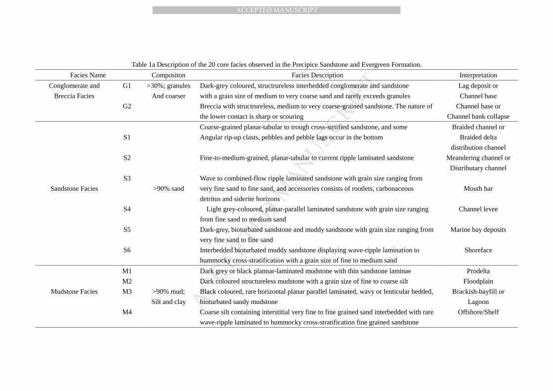
Table 1 Description of the 20 core facies observed in the Precipice Sandstone

and Evergreen Formation.

Table 2 The relationship between core facies and wireline log facies from the

five key core wells.

Table 3 A summary of wireline log characteristics for the ten wireline log facies.

Table 4 Statistical data from the Markvo Chain Analysis: (A) Transition count

matrix; (B) Transition probability matrix; and, (C) Difference matrix.

Table 5 Plot of the wireline log facies from the MLPC, compared with the core-

defined facies, showing the proportion of correctly predicted facies on the

diagonal and miss-classified facies in the off diagonal.

MANUSCRIP

T

ACCEPTED

ACCEPTED MANUSCRIPT

Table 1a Description of the 20 core facies observed in the Precipice Sandstone and Evergreen Formation.

Facies Name Compositon Facies Description Interpretation

Conglomerate and

Breccia Facies

G1 >30%; granules

And coarser

Dark-grey coloured, structrureless interbedded conglomerate and sandstone

with a grain size of medium to very coarse sand and rarely exceeds granules

Lag deposit or

Channel base

G2 Breccia with structrureless, medium to very coarse-grained sandstone. The nature of

the lower contact is sharp or scouring

Channel base or

Channel bank collapse

Sandstone Facies

S1

>90% sand

Coarse-grained planar-tabular to trough cross-strtified sandstone, and some

Angular rip-up clasts, pebbles and pebble lags occur in the bottom

Braided channel or

Braided delta

distribution channel

S2 Fine-to-medium-grained, planar-tabular to current ripple laminated sandstone Meandering channel or

Distributary channel

S3 Wave to combined-flow ripple laminated sandstone with grain size ranging from

very fine sand to fine sand, and accessories consists of rootlets, carbonaceous

detritus and siderite horizons

Mouth bar

S4 Light grey-coloured, planar-parallel laminated sandstone with grain size ranging

from fine sand to medium sand

Channel levee

S5 Dark-grey, bioturbated sandstone and muddy sandstone with grain size ranging from

very fine sand to fine sand

Marine bay deposits

S6 Interbedded bioturbated muddy sandstone displaying wave-ripple lamination to

hummocky cross-stratification with a grain size of fine to medium sand

Shoreface

Mudstone Facies

M1

>90% mud;

Silt and clay

Dark grey or black plannar-laminated mudstone with thin sandstone laminae Prodelta

M2 Dark coloured structureless mudstone with a grain size of fine to coarse silt Floodplain

M3 Black coloured, rare horizontal planar parallel laminated, wavy or lenticular bedded,

bioturbated sandy mudstone

Brackish-bayfill or

Lagoon

M4 Coarse silt containing interstitial very fine to fine grained sand interbedded with rare

wave-ripple laminated to hummocky cross-stratification fine grained sandstone

Offshore/Shelf

MANUSCRIP

T

ACCEPTED

ACCEPTED MANUSCRIPT

Table 1b Description of the 20 core facies observed in the Precipice Sandstone and Evergreen Formation.

Facies Name Compositon Facies Description Interpretation

Heterolithics Facies

SM1

>10% and <90%

sand

Light-grey to dark-grey coloured, medium to coarse silt interbedded with very fine

to fine grained sand and described as sand-diminated heterolithics

Proximal delta front

SM2 Less sand than mud (70%>sand>30%), heterolithics with current to combined flow

ripple lamination, wave ripple lamination and synaereses cracks

Distal delta front

SM3 A black or dark-grey colour, wave-influenced mud-dominated heterolithics with

medium to coarse silt and very fine to fine grained sand

Prosimal prodelta

SM4 Tide-influenced mixed heterolithics with more intense bioturbation accessories

consist of carbonaceous detritus, rootlets and rare sideritized horizons

Tidal flats

SM5 Grey colour, inclined heterolithics stratification with current ripples flashers, wavy,

and lenticular bedding and rare synaereses cracks

Tide-fluvial channel

Organic and

Miscellaneous Facies

O1

Bituminous to sub-bituminous coal Peat mire or

Interdistributary bay

O2 Grey colour, very fine silt to fine-grained sand, carbonaceous sandstone and siltstone Floodplain or

Interdistributary bay

O3 Reddish brown colour ironstone (oolithic or cemented) Lagoon or Restricted

embayment

MANUSCRIP

T

ACCEPTED

ACCEPTED MANUSCRIPT

Table 2 The relationship between core facies and wireline log facies from the five key core wells. Core facies Key well thickness Porosity/% Permeability/ mD N Logging

Facies Feature of GR curve shape

G1 3 0.25-1.2/0.83 \ \ 6 Not Find Smooth concave bell shape G2 2 0.17-0.8/0.41 \ \ 5 Not Find Smooth concave bell shape S1 5 0.2-77.2/12.59 17.7-21.3/19.89 3.18-2500/2100 19 SA Smooth cylindrical shape S2 5 0.35-18.7/4.54 6.4-12.2/10.7 0.004-0.8/0.61 32 SB Smooth concave bell shape S3 5 0.2-10.33/2.26 5.9-11.2/9.05 0.002-0.23/0.038 64

SC Smooth concave funnel shape

S4 2 0.18-4.85/1.30 \ \ 19 Erratic concave funnel shape S5 3 0.1-3.2/0.98 8.1-9.1/8.5 0.085-0.26/0.18 11

SD Smooth concave funnel shape

S6 1 1.30-7.12/3.29 \ \ 4 Erratic concave funnel shape M1 5 0.14-3.65/1.43 \ \ 29

MA Erratic line shape

M2 4 0.12-7.60/1.15 \ \ 50 Smooth line shape M3 3 0.23-1.90/0.80 \ \ 10

MB Erratic line shape

M4 1 0.53-4.13/2.33 \ \ 2 Smooth line shape SM1 5 0.18-4.84/1.53 4.6-11.4/9.3 0.013-0.069/0.03 53

SMA Smooth concave egg shape

SM2 4 0.25-5.70/2.08 5.2-9.4/8.15 0.002-0.051/0.028 31 Erratic concave egg shape SM3 5 0.16-10.6/1.49 5.1-7.2/7.38 0.001-0.032/0.023 70

SMB Erratic line shape

SM4 5 0.11-5.50/1.54 2.8-6.8/5.7 0.001-0.029/0.021 94 Erratic line shape SM5 1 0.4-0.6/0.5 \ \ 2 Not Find Erratic concave egg shape O1 4 0.05-0.91/0.22 \ \ 21 OA Smooth convex egg shape O2 4 0.1-1.3/0.32 6.3-6.9/6.4 0.001-0.005/0.003 15 Not Find Erratic concave funnel shape O3 5 0.05-1.35/0.44 6.8-7.9/7.2 <0.001 33 OB Smooth convex egg shape

Note: 0.25-1.2/0.83: the minimum –maximum thickness/ the average thickness; N: the frequency of each core facies; 17.7-21.3/19.89, 3.18-2500/2100: the value reach the 25 th and 75 th percentiles of cumulative percentage/ average value

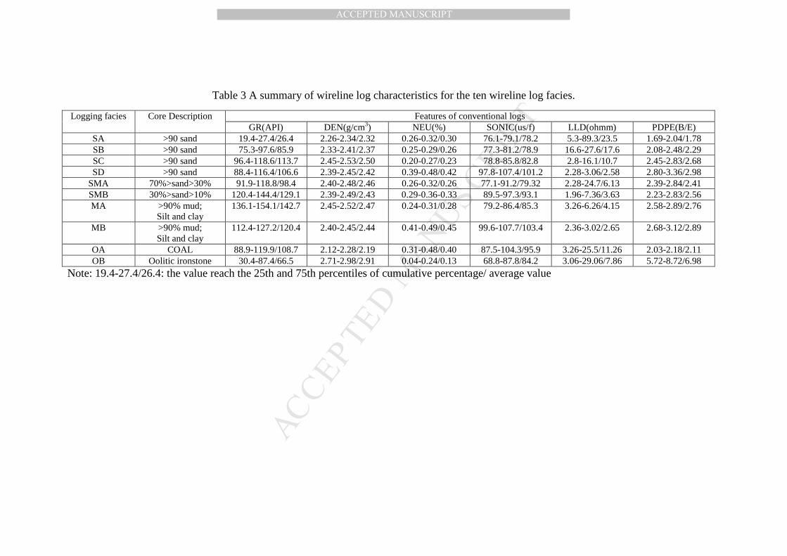
MANUSCRIP

T

ACCEPTED

ACCEPTED MANUSCRIPT

Table 3 A summary of wireline log characteristics for the ten wireline log facies.

Logging facies Core Description Features of conventional logs GR(API) DEN(g/cm3) NEU(%) SONIC(us/f) LLD(ohmm) PDPE(B/E)

SA >90 sand 19.4-27.4/26.4 2.26-2.34/2.32 0.26-0.32/0.30 76.1-79.1/78.2 5.3-89.3/23.5 1.69-2.04/1.78 SB >90 sand 75.3-97.6/85.9 2.33-2.41/2.37 0.25-0.29/0.26 77.3-81.2/78.9 16.6-27.6/17.6 2.08-2.48/2.29 SC >90 sand 96.4-118.6/113.7 2.45-2.53/2.50 0.20-0.27/0.23 78.8-85.8/82.8 2.8-16.1/10.7 2.45-2.83/2.68 SD >90 sand 88.4-116.4/106.6 2.39-2.45/2.42 0.39-0.48/0.42 97.8-107.4/101.2 2.28-3.06/2.58 2.80-3.36/2.98

SMA 70%>sand>30% 91.9-118.8/98.4 2.40-2.48/2.46 0.26-0.32/0.26 77.1-91.2/79.32 2.28-24.7/6.13 2.39-2.84/2.41 SMB 30%>sand>10% 120.4-144.4/129.1 2.39-2.49/2.43 0.29-0.36-0.33 89.5-97.3/93.1 1.96-7.36/3.63 2.23-2.83/2.56 MA >90% mud;

Silt and clay 136.1-154.1/142.7 2.45-2.52/2.47 0.24-0.31/0.28 79.2-86.4/85.3 3.26-6.26/4.15 2.58-2.89/2.76

MB >90% mud; Silt and clay

112.4-127.2/120.4 2.40-2.45/2.44 0.41-0.49/0.45 99.6-107.7/103.4 2.36-3.02/2.65 2.68-3.12/2.89

OA COAL 88.9-119.9/108.7 2.12-2.28/2.19 0.31-0.48/0.40 87.5-104.3/95.9 3.26-25.5/11.26 2.03-2.18/2.11 OB Oolitic ironstone 30.4-87.4/66.5 2.71-2.98/2.91 0.04-0.24/0.13 68.8-87.8/84.2 3.06-29.06/7.86 5.72-8.72/6.98

Note: 19.4-27.4/26.4: the value reach the 25th and 75th percentiles of cumulative percentage/ average value

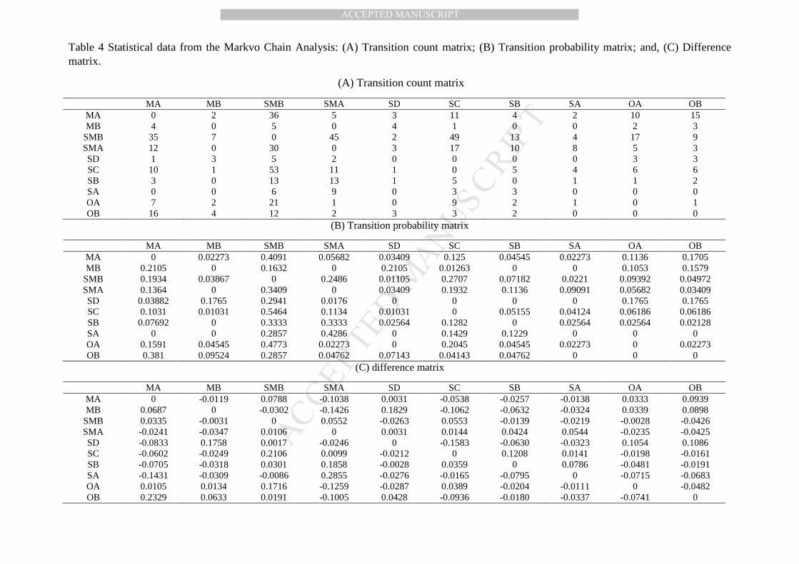
MANUSCRIP

T

ACCEPTED

ACCEPTED MANUSCRIPT

Table 4 Statistical data from the Markvo Chain Analysis: (A) Transition count matrix; (B) Transition probability matrix; and, (C) Difference matrix.

(A) Transition count matrix

MA MB SMB SMA SD SC SB SA OA OB MA 0 2 36 5 3 11 4 2 10 15 MB 4 0 5 0 4 1 0 0 2 3

SMB 35 7 0 45 2 49 13 4 17 9 SMA 12 0 30 0 3 17 10 8 5 3 SD 1 3 5 2 0 0 0 0 3 3 SC 10 1 53 11 1 0 5 4 6 6 SB 3 0 13 13 1 5 0 1 1 2 SA 0 0 6 9 0 3 3 0 0 0 OA 7 2 21 1 0 9 2 1 0 1 OB 16 4 12 2 3 3 2 0 0 0

(B) Transition probability matrix

MA MB SMB SMA SD SC SB SA OA OB MA 0 0.02273 0.4091 0.05682 0.03409 0.125 0.04545 0.02273 0.1136 0.1705 MB 0.2105 0 0.1632 0 0.2105 0.01263 0 0 0.1053 0.1579

SMB 0.1934 0.03867 0 0.2486 0.01105 0.2707 0.07182 0.0221 0.09392 0.04972 SMA 0.1364 0 0.3409 0 0.03409 0.1932 0.1136 0.09091 0.05682 0.03409 SD 0.03882 0.1765 0.2941 0.0176 0 0 0 0 0.1765 0.1765 SC 0.1031 0.01031 0.5464 0.1134 0.01031 0 0.05155 0.04124 0.06186 0.06186 SB 0.07692 0 0.3333 0.3333 0.02564 0.1282 0 0.02564 0.02564 0.02128 SA 0 0 0.2857 0.4286 0 0.1429 0.1229 0 0 0 OA 0.1591 0.04545 0.4773 0.02273 0 0.2045 0.04545 0.02273 0 0.02273 OB 0.381 0.09524 0.2857 0.04762 0.07143 0.04143 0.04762 0 0 0

(C) difference matrix

MA MB SMB SMA SD SC SB SA OA OB MA 0 -0.0119 0.0788 -0.1038 0.0031 -0.0538 -0.0257 -0.0138 0.0333 0.0939 MB 0.0687 0 -0.0302 -0.1426 0.1829 -0.1062 -0.0632 -0.0324 0.0339 0.0898

SMB 0.0335 -0.0031 0 0.0552 -0.0263 0.0553 -0.0139 -0.0219 -0.0028 -0.0426 SMA -0.0241 -0.0347 0.0106 0 0.0031 0.0144 0.0424 0.0544 -0.0235 -0.0425 SD -0.0833 0.1758 0.0017 -0.0246 0 -0.1583 -0.0630 -0.0323 0.1054 0.1086 SC -0.0602 -0.0249 0.2106 0.0099 -0.0212 0 0.1208 0.0141 -0.0198 -0.0161 SB -0.0705 -0.0318 0.0301 0.1858 -0.0028 0.0359 0 0.0786 -0.0481 -0.0191 SA -0.1431 -0.0309 -0.0086 0.2855 -0.0276 -0.0165 -0.0795 0 -0.0715 -0.0683 OA 0.0105 0.0134 0.1716 -0.1259 -0.0287 0.0389 -0.0204 -0.0111 0 -0.0482 OB 0.2329 0.0633 0.0191 -0.1005 0.0428 -0.0936 -0.0180 -0.0337 -0.0741 0

MANUSCRIP

T

ACCEPTED

ACCEPTED MANUSCRIPT

Table 5 Plot of the wireline log facies from the MLPC, compared with the core-defined facies, showing the proportion of correctly predicted facies on the diagonal and miss-classified facies in the off diagonal. Core-defiend

facies Predicted litofacies Core

total Proportion of correct

predictions MA MB SMB SMA SD SC SB SA OA OB

MA 690 212 3 8 913 75.57503 MB 8 171 18 7 204 83.82353

SMB 197 2531 4 50 2782 90.97771 SMA 292 710 66 1068 66.47940 SD 12 35 143 190 75.26316 SC 73 84 468 30 655 71.45038 SB 33 114 1922 5 2074 92.67117 SA 35 1 4152 4188 99.14040 OA 5 18 23 78.26087 OB 2 1 94 97 96.90722

Predicted total 895 183 3282 869 150 708 1954 4157 18 94 12194 83.0549 Predicted/core 0.980 0.897 1.179 0.814 0.789 1.081 0.942 0.993 0.783 0.969

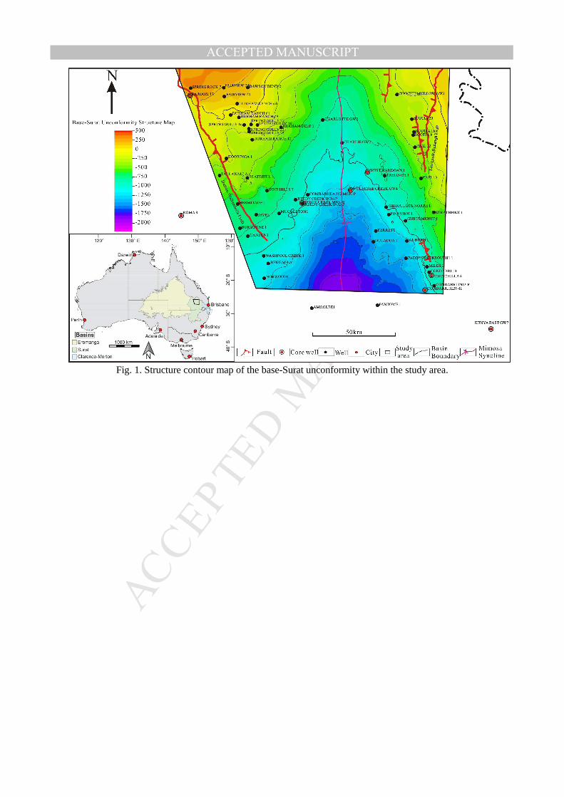
MANUSCRIP

T

ACCEPTED

ACCEPTED MANUSCRIPT

Fig. 1. Structure contour map of the base-Surat unconformity within the study area.

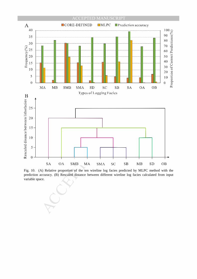
MANUSCRIP

T

ACCEPTED

ACCEPTED MANUSCRIPT

Fig. 10. (A) Relative proportion of the ten wireline log facies predicted by MLPC method with the prediction accuracy. (B) Rescaled distance between different wireline log facies calculated from input variable space.

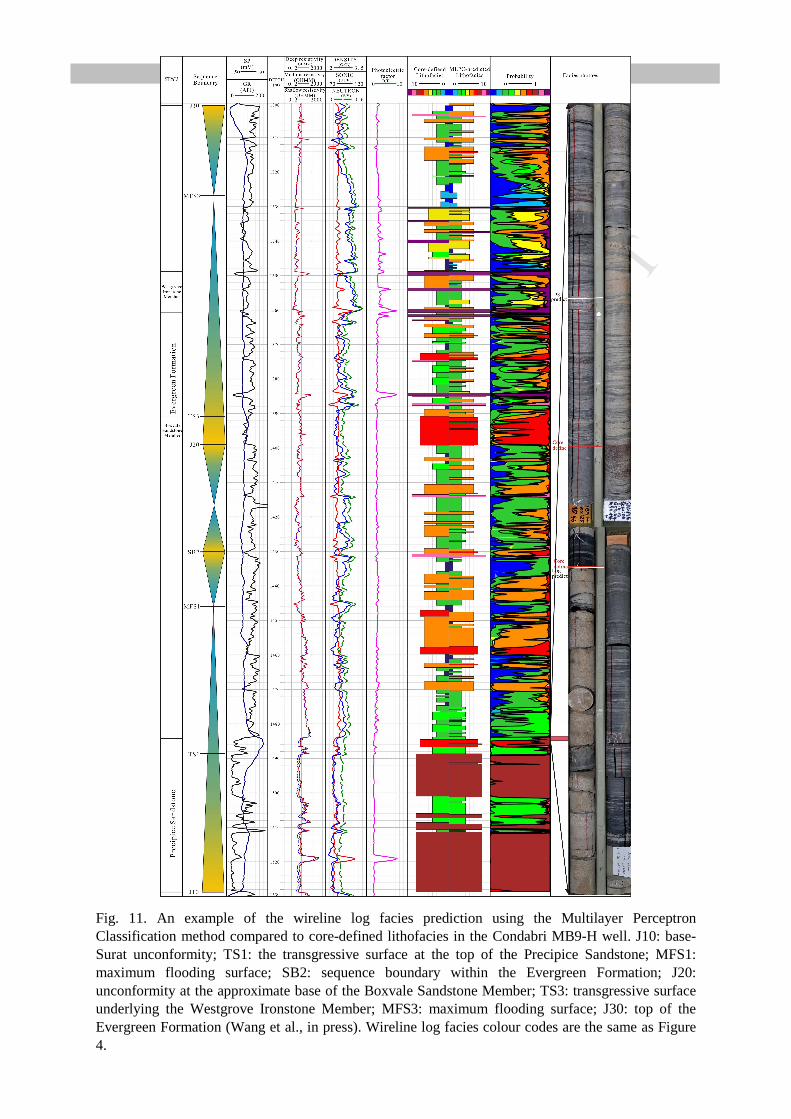
MANUSCRIP

T

ACCEPTED

ACCEPTED MANUSCRIPT

Fig. 11. An example of the wireline log facies prediction using the Multilayer Perceptron Classification method compared to core-defined lithofacies in the Condabri MB9-H well. J10: base-Surat unconformity; TS1: the transgressive surface at the top of the Precipice Sandstone; MFS1: maximum flooding surface; SB2: sequence boundary within the Evergreen Formation; J20: unconformity at the approximate base of the Boxvale Sandstone Member; TS3: transgressive surface underlying the Westgrove Ironstone Member; MFS3: maximum flooding surface; J30: top of the Evergreen Formation (Wang et al., in press). Wireline log facies colour codes are the same as Figure 4.

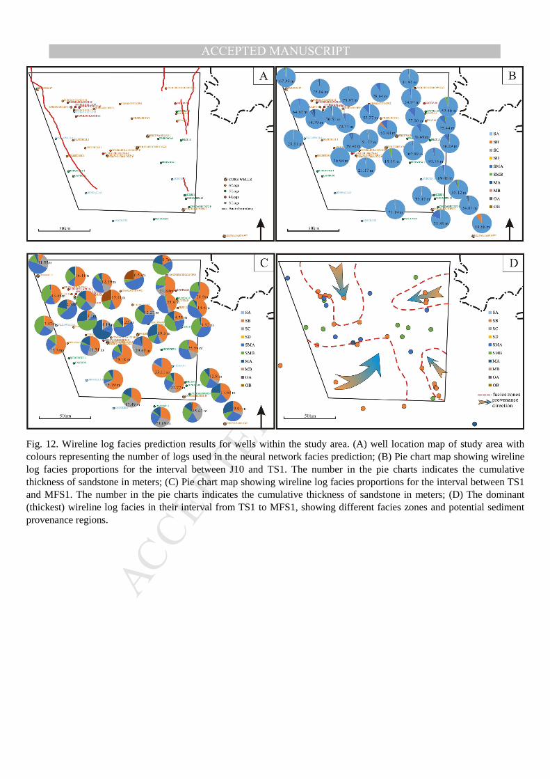
MANUSCRIP

T

ACCEPTED

ACCEPTED MANUSCRIPT

Fig. 12. Wireline log facies prediction results for wells within the study area. (A) well location map of study area with colours representing the number of logs used in the neural network facies prediction; (B) Pie chart map showing wireline log facies proportions for the interval between J10 and TS1. The number in the pie charts indicates the cumulative thickness of sandstone in meters; (C) Pie chart map showing wireline log facies proportions for the interval between TS1 and MFS1. The number in the pie charts indicates the cumulative thickness of sandstone in meters; (D) The dominant (thickest) wireline log facies in their interval from TS1 to MFS1, showing different facies zones and potential sediment provenance regions.

MANUSCRIP

T

ACCEPTED

ACCEPTED MANUSCRIPT

Fig. 13. (A) Final convergence error. (B) Prediction accuracy based on the input log types used for wireline log facies prediction.

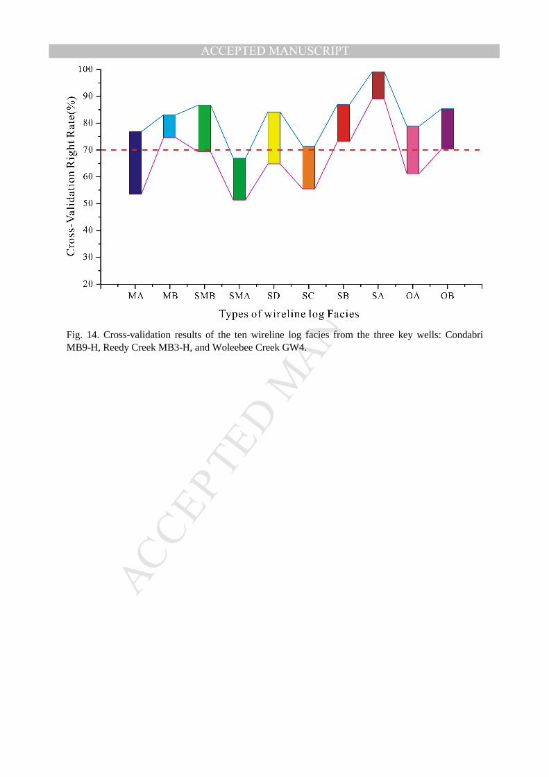
MANUSCRIP

T

ACCEPTED

ACCEPTED MANUSCRIPT

Fig. 14. Cross-validation results of the ten wireline log facies from the three key wells: Condabri MB9-H, Reedy Creek MB3-H, and Woleebee Creek GW4.

MANUSCRIP

T

ACCEPTED

ACCEPTED MANUSCRIPT

Fig. 15. Facies distribution maps based on wireline log facies determined from neural networks. (A) The Precipice Sandstone. The zero-thickness boundary shown in red is based on seismic interpretation (B) The Lower Evergreen Formation.

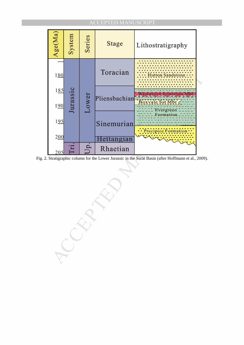
MANUSCRIP

T

ACCEPTED

ACCEPTED MANUSCRIPT

Fig. 2. Stratigraphic column for the Lower Jurassic in the Surat Basin (after Hoffmann et al., 2009).

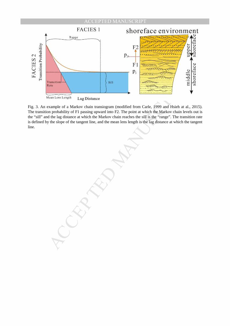
MANUSCRIP

T

ACCEPTED

ACCEPTED MANUSCRIPT

Fig. 3. An example of a Markov chain transiogram (modified from Carle, 1999 and Hsieh at al., 2015). The transition probability of F1 passing upward into F2. The point at which the Markov chain levels out is the “sill” and the lag distance at which the Markov chain reaches the sill is the “range”. The transition rate is defined by the slope of the tangent line, and the mean lens length is the lag distance at which the tangent line.

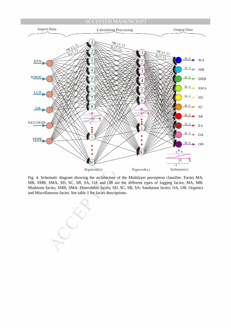
MANUSCRIP

T

ACCEPTED

ACCEPTED MANUSCRIPT

Fig. 4. Schematic diagram showing the architecture of the Multilayer perceptron classifier. Facies MA, MB, SMB, SMA, SD, SC, SB, SA, OA and OB are the different types of logging facies; MA, MB: Mudstone facies; SMB, SMA: Heterolithic facies; SD, SC, SB, SA: Sandstone facies; OA, OB: Organics and Miscellaneous facies. See table 1 for facies descriptions.

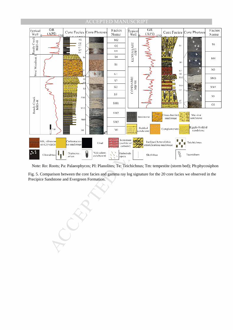
MANUSCRIP

T

ACCEPTED

ACCEPTED MANUSCRIPT

Note: Ro: Roots; Pa: Palaeophycos; PI: Planolites; Te: Teichichnus; Tm: tempestite (storm bed); Ph:phycosiphon

Fig. 5. Comparison between the core facies and gamma ray log signature for the 20 core facies we observed in the Precipice Sandstone and Evergreen Formation.

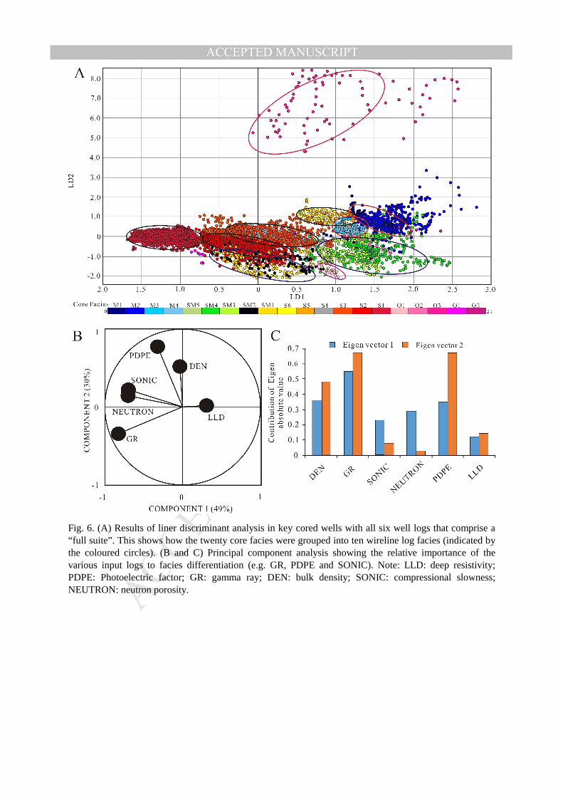
MANUSCRIP

T

ACCEPTED

ACCEPTED MANUSCRIPT

Fig. 6. (A) Results of liner discriminant analysis in key cored wells with all six well logs that comprise a “full suite”. This shows how the twenty core facies were grouped into ten wireline log facies (indicated by the coloured circles). (B and C) Principal component analysis showing the relative importance of the various input logs to facies differentiation (e.g. GR, PDPE and SONIC). Note: LLD: deep resistivity; PDPE: Photoelectric factor; GR: gamma ray; DEN: bulk density; SONIC: compressional slowness; NEUTRON: neutron porosity.

MANUSCRIP

T

ACCEPTED

ACCEPTED MANUSCRIPT

Fig. 7. Rider chart showing the recognition models for the ten types of wireline log facies. The average value of each log in the different wireline log facies is displayed.

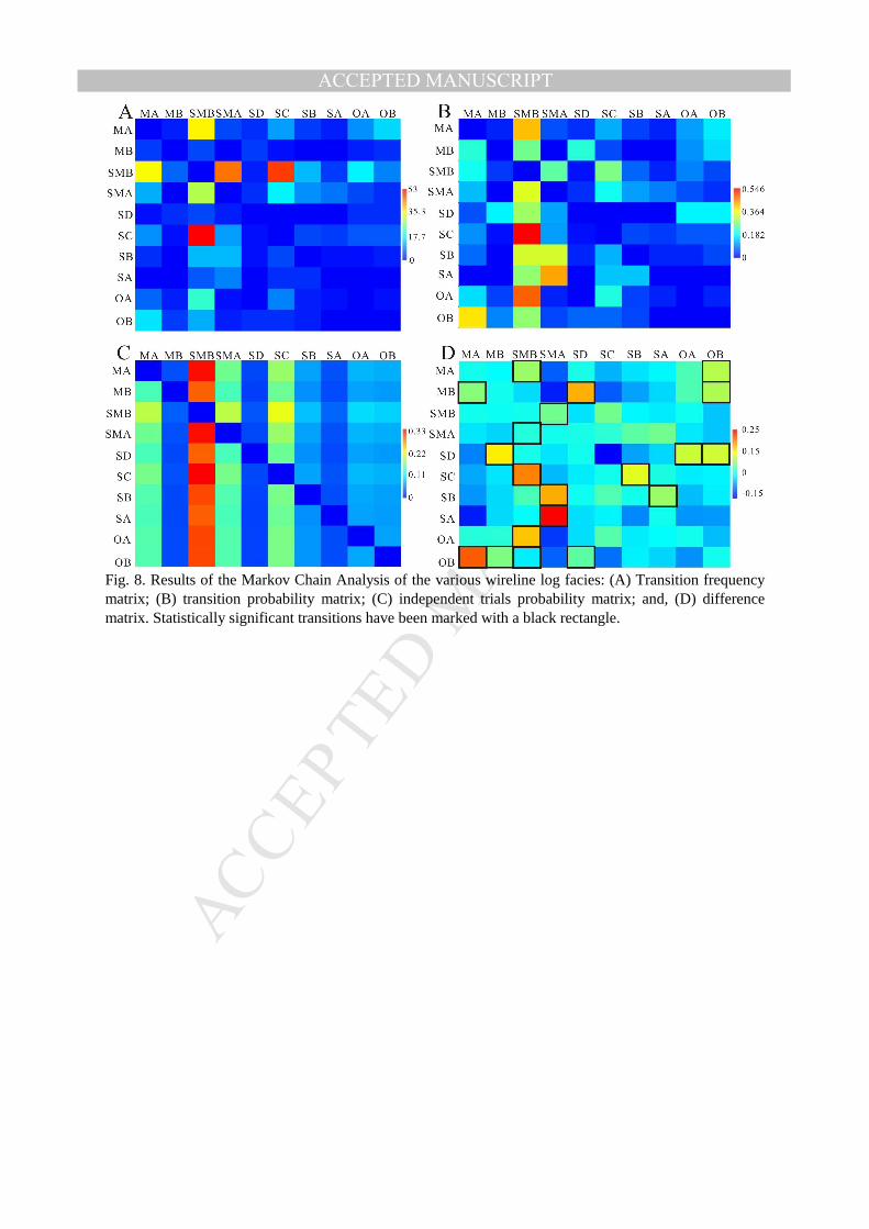
MANUSCRIP

T

ACCEPTED

ACCEPTED MANUSCRIPT

Fig. 8. Results of the Markov Chain Analysis of the various wireline log facies: (A) Transition frequency matrix; (B) transition probability matrix; (C) independent trials probability matrix; and, (D) difference matrix. Statistically significant transitions have been marked with a black rectangle.

MANUSCRIP

T

ACCEPTED

ACCEPTED MANUSCRIPT

Fig. 9. Conceptual models of the five facies associations determined by MCA. An approximate scale indicates the thickness of individual facies. The arrow shows the transitions from one facies to another. The number on the arrow represents the level of significance of facies transitions (based on the difference matrix). (A) Channel Complex Association. (B) Delta Plain Association. (C) Subaqeous Delta Association. (D) Shoreface Association. (E) Tidal Flats and Channels Association.

MANUSCRIP

T

ACCEPTED

ACCEPTED MANUSCRIPT

Highlights

• Facies analysis of the Precipice Sandstone and Evergreen Formation • Core facies simplified into a set of wireline log facies (WLF) with unique

petrophysical properties using statistical methods. • Facies transition significance determined from Markov Chain Analysis used to

group the WLF into facies associations. • Neural networks trained with core and Markov Chain results for facies prediction

in wells with wireline logs but no core. • Facies prediction from logs demonstrate a high accuracy, and thus provide

important input for reservoir modelling for CO2 storage assessment.