Using Microdata AccessWith ACS 1-Year Estimates – Public Use Microdata Sample

data.census.gov/mdat

1v1: November 07, 2019

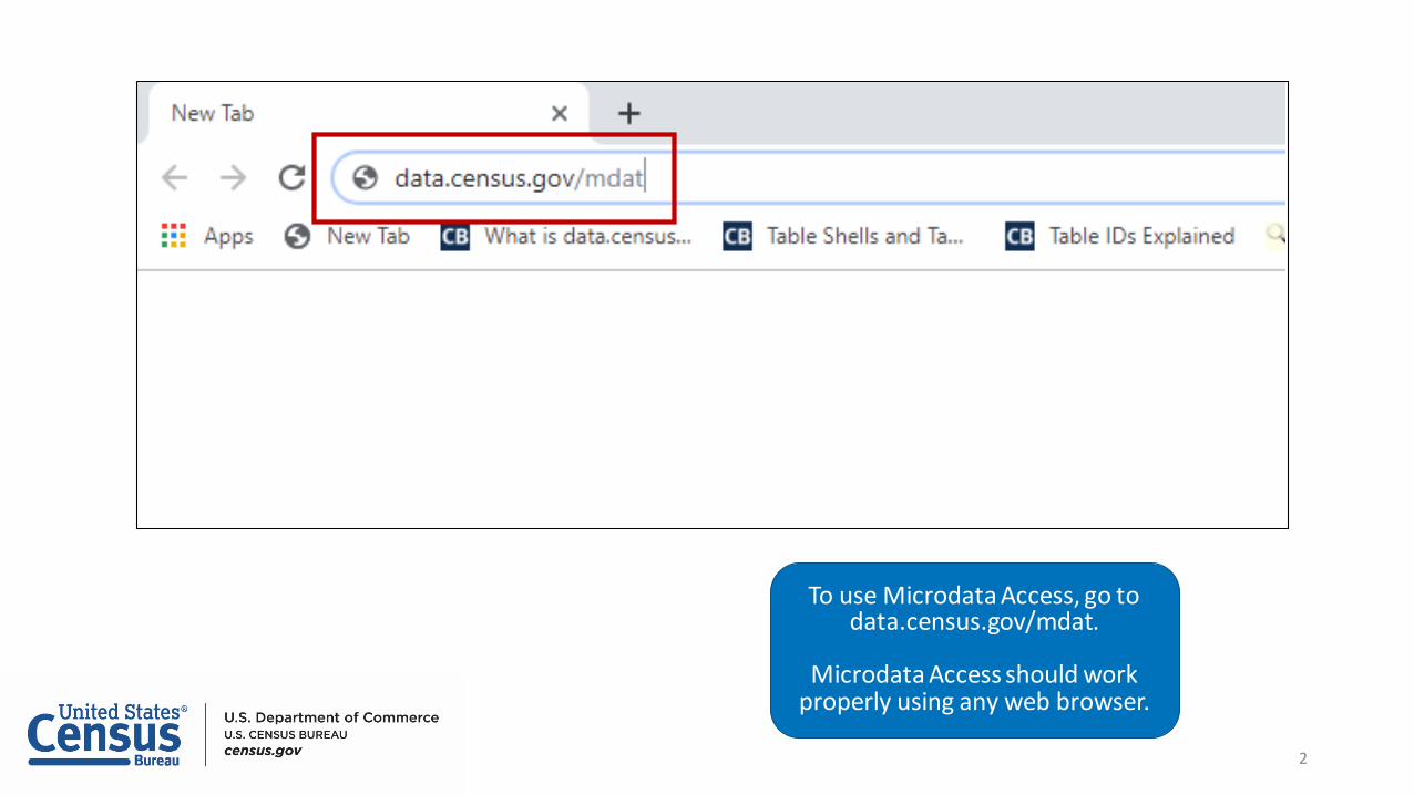
To use Microdata Access, go to data.census.gov/mdat.

Microdata Access should work properly using any web browser.

2

The landing page allows you to select your dataset and vintage.

3

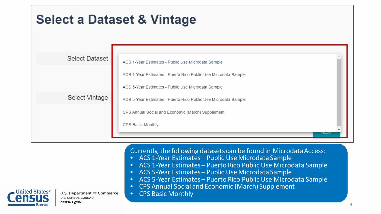
Currently, the following datasets can be found in Microdata Access:• ACS 1-Year Estimates – Public Use Microdata Sample• ACS 1-Year Estimates – Puerto Rico Public Use Microdata Sample• ACS 5-Year Estimates – Public Use Microdata Sample• ACS 5-Year Estimates – Puerto Rico Public Use Microdata Sample• CPS Annual Social and Economic (March) Supplement• CPS Basic Monthly

4

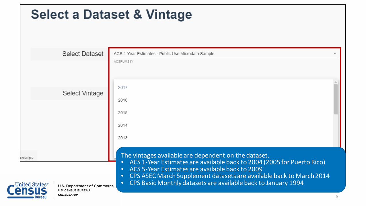
The vintages available are dependent on the dataset.• ACS 1-Year Estimates are available back to 2004 (2005 for Puerto Rico)• ACS 5-Year Estimates are available back to 2009• CPS ASEC March Supplement datasets are available back to March 2014• CPS Basic Monthlydatasets are available back to January 1994

5

6

For this walkthrough, we’ll use the 2017 ACS 1-Year Estimates. Once theseare selected, hit the NEXT button found in the lower right of the screen.

7

The SELECT VARIABLES screen is the next screen that appears. You canchoose the variables that you need by clicking the checkbox next to it. Tofind the variables more quickly, you can use the search bar to search for thedesired variable. You can view specific details about the variable by clickingon the DETAILS dropdown.

8

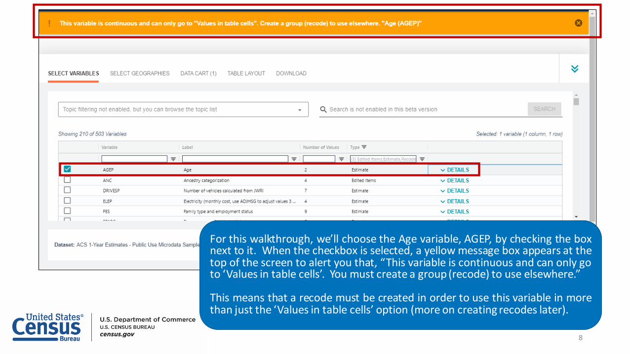
For this walkthrough, we’ll choose the Age variable, AGEP, by checking the boxnext to it. When the checkbox is selected, a yellow message box appears at thetop of the screen to alert you that, “This variable is continuous and can only goto ‘Values in table cells’. You must create a group (recode) to use elsewhere.”

This means that a recode must be created in order to use this variable in morethan just the ‘Values in table cells’ option (more on creating recodes later).

9

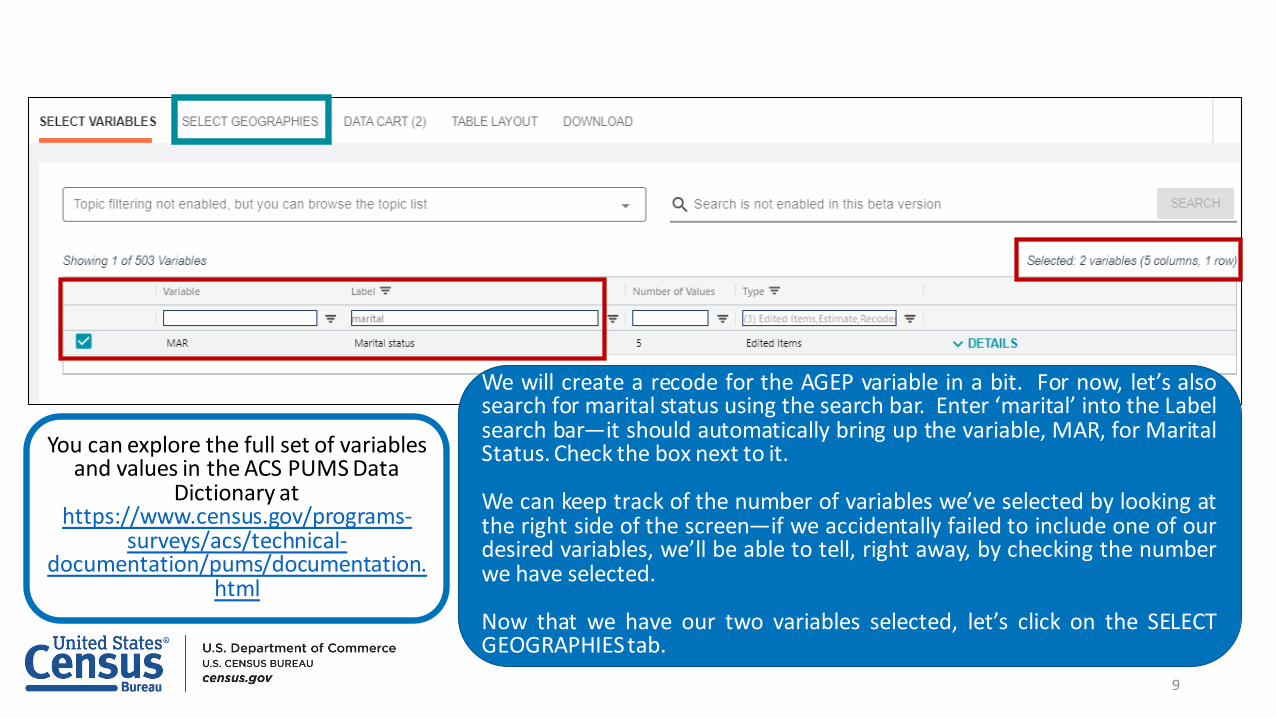
We will create a recode for the AGEP variable in a bit. For now, let’s alsosearch for marital status using the search bar. Enter ‘marital’ into the Labelsearch bar—it should automatically bring up the variable, MAR, for MaritalStatus. Check the box next to it.

We can keep track of the number of variables we’ve selected by looking atthe right side of the screen—if we accidentally failed to include one of ourdesired variables, we’ll be able to tell, right away, by checking the numberwe have selected.

Now that we have our two variables selected, let’s click on the SELECTGEOGRAPHIEStab.

You can explore the full set of variables and values in the ACS PUMS Data

Dictionary at https://www.census.gov/programs-

surveys/acs/technical-documentation/pums/documentation.

html

10

Now that we’re on the SELECT GEOGRAPHIES tab, let’s choose our geography. Nation, State and Public UseMicrodata Area (PUMA) geographies are available. If you do not select a geography, Nation will be used asthe default geography.

Other geographies will be enabled in the future. Once the other geographies are enabled, you’ll see that thelist is tailored according to the survey being used.

For this example, let’s click on State. Next, we’ll check the box next to California.

11

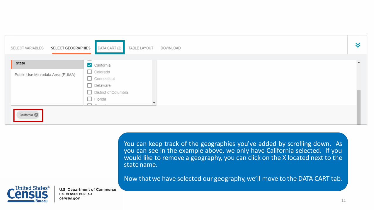
You can keep track of the geographies you’ve added by scrolling down. Asyou can see in the example above, we only have California selected. If youwould like to remove a geography, you can click on the X located next to thestatename.

Now that we have selected our geography, we’ll move to the DATA CART tab.

12

This is how your DATA CART tab should look. Your selected variables should be displayed on the left side of the screen(highlighted in the green box). The information for the variable you have highlighted on the left will be displayed onthe right side of the screen (highlighted in the purple box)—this section is used to create the recodes. In our case,right now we have the AGEP variable selected, so we can create a recode for it. If we were to select the MAR variable,we could createa recode for that, as well.

13

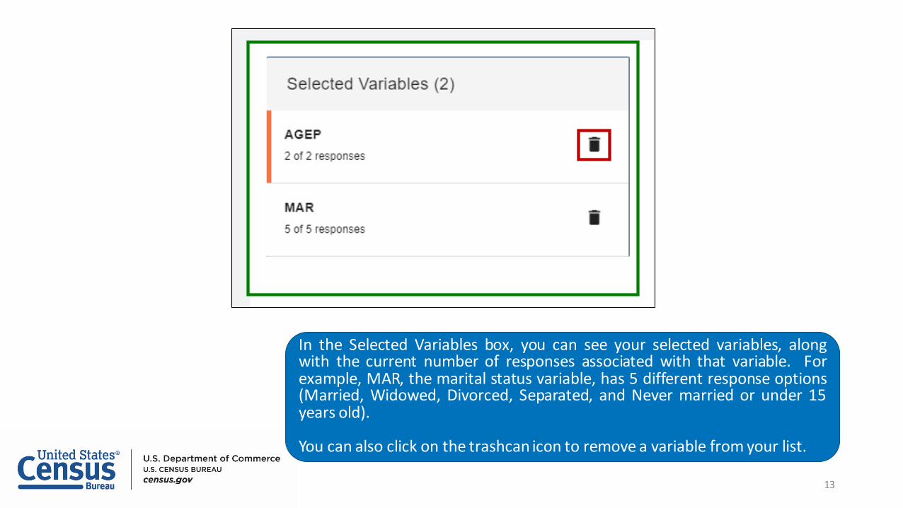
In the Selected Variables box, you can see your selected variables, alongwith the current number of responses associated with that variable. Forexample, MAR, the marital status variable, has 5 different response options(Married, Widowed, Divorced, Separated, and Never married or under 15years old).

You can also click on the trashcan icon to remove a variable from your list.

14

In the Age (AGEP) box, you’ll find the current information about the variable,such as the Response Label and the value range.

This is where we will create a recode of the Age (AGEP) variable.

To create the recode, select the + CREATE CUSTOM GROUP button.

15

As soon as you click the + CREATE CUSTOM GROUP button, a new variable(the recode you have created) will be added to the Selected Variables list.Our recode is called AGEP_RC1. You’ll also notice that we now have threevariables in our DATA CART.

16

Before we do anything else, let’s go over some things about this recode.First, we can rename the recode to something that makes sense. Let’s callours “Age Recode”—click on, or next to, the “Not Elsewhere Classified” textin the Group Label box, delete it, and type “Age Recode” in that spot.

17

You can also change the Recode Label by selecting the pencil icon next to theAge recode text. Once you are happy with the label, click on the check markin the green circle.

18

The site offers two ways to create custom groups of continuous variables. You can manually specify each grouping or you can use theAuto Group feature. For this example, we will use the Auto Group feature. Click on the AUTO GROUP button. This will bring up theAuto Group Variable box where you select your starting and ending values, as well as the spacing for the groups you would like to have.

Let’s keep the starting value as 1 and the ending value as 99. However, let’s change the number of groups from ‘1’ to ’10’. This will giveus the full range of values split into groups of 10 (i.e., between 1 and 10, between 11 and 20, etc.) Then hit the AUTO GROUP button.

If you’d like to cancel the auto grouping, hit the CANCEL button.

Note: For an example of manually specifying each grouping, go to page 37 of this document, “Manually Specifying a CustomGroup.”

19

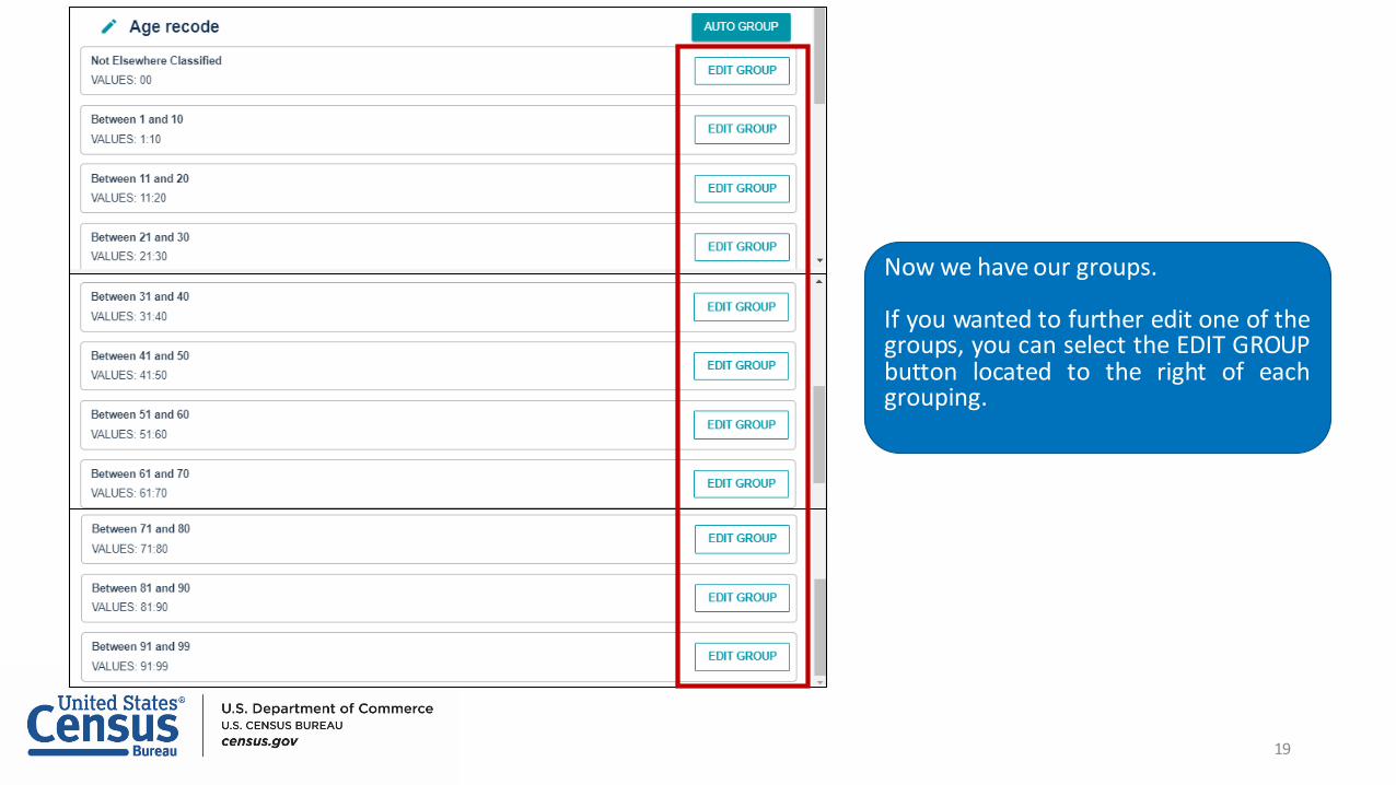
Now we have our groups.

If you wanted to further edit one of thegroups, you can select the EDIT GROUPbutton located to the right of eachgrouping.

20

Now that we have our groups, let’s move to the TABLE LAYOUT tab. This tab provides a preview ofyour table. As you can see, we have California placed as our row variable and marital status placed asour column variable. The ??? act as placeholders for the data that will populate the table.

You can make modifications to the table by clicking on a row header or column header, holding themouse, and dragging it to the spot you would like it to be.

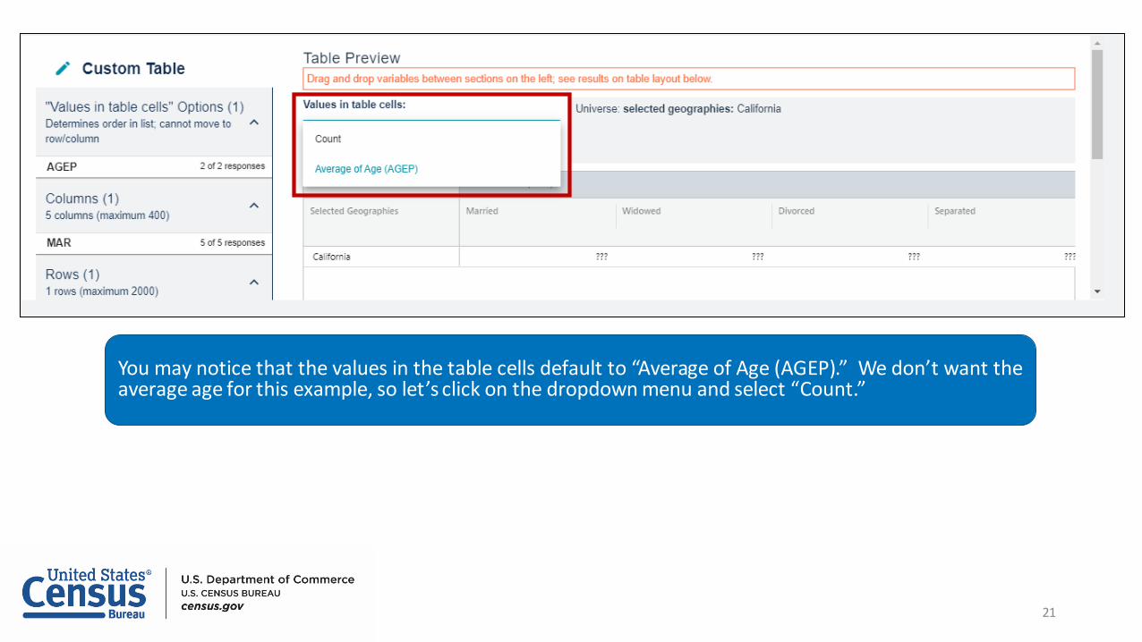
21

You may notice that the values in the table cells default to “Average of Age (AGEP).” We don’t want theaverage age for this example, so let’s click on the dropdown menu and select “Count.”

22

You may notice that our preview table is only using the geography we selected (California) and one ofthe variables that we selected (MAR, or marital status). To add our age recodes, scroll down until yousee the AGEP_RC1 variable. Click on the AGEP_RC1 text. While holding the click on your mouse, dragit over to the table preview. Let’s drop it right underneath the cell for California.

Drop it here

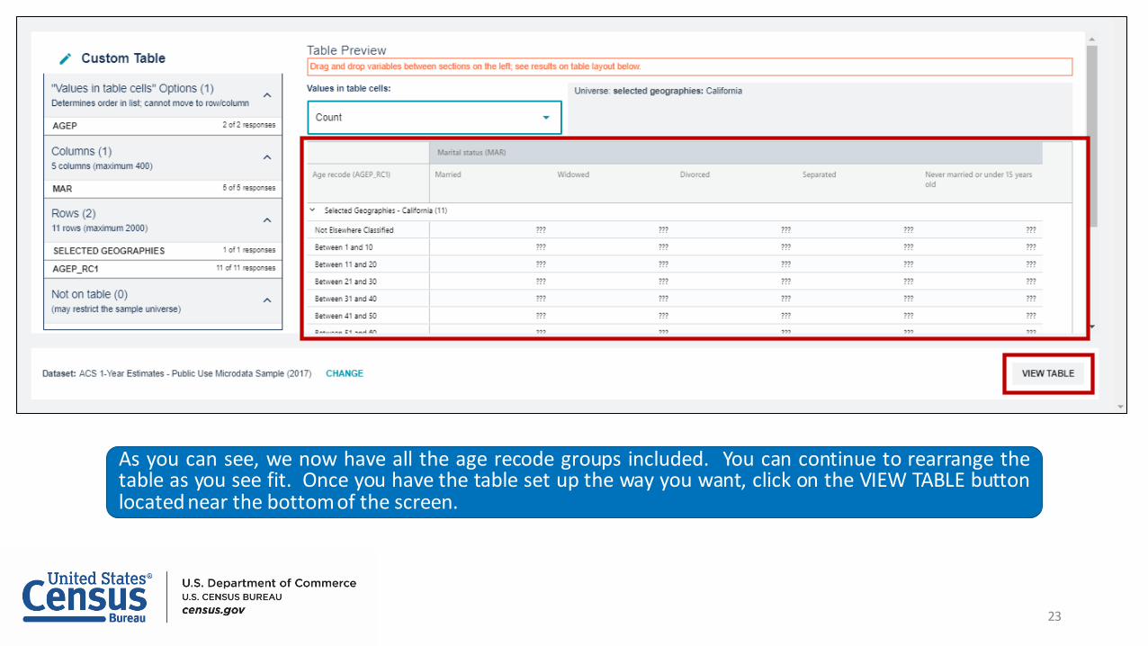
23

As you can see, we now have all the age recode groups included. You can continue to rearrange thetable as you see fit. Once you have the table set up the way you want, click on the VIEW TABLE buttonlocated near the bottom of the screen.

24

This screen has a lot of different options on it. Let’s take a few moments to go over the different thingsthat are included on it.

25

First and foremost, we have our table displayed at the bottom of the page. As you can see, the table ispopulated with the actual estimates instead of the question marks we saw on the preview. Right abovethe table, you can see that our Universe is our selected geography, California.

26

Now back to the top of the screen. You have the option to change the dataset, vintage, geography, andweighting.

You should always confirm that the PUMS person weight is applied if the values represent a personvariable and the Housing Weight is applied if the values represent a household variable. For thisexample, the appropriate weighting is the PUMS person weight, since we are using person-levelvariables.

27

You can also move the variables around from a row to a column, or vice versa, using the black variablepills (examples highlighted in the purple box). If you need to add a variable (or remove one), you canclick on the + in the circle—this will take you back to the earlier screen that lists all the variables.

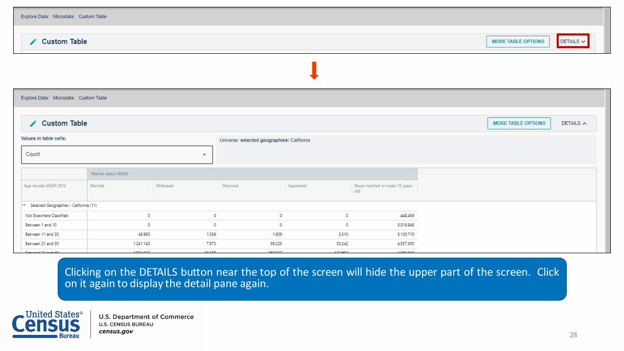
28

Clicking on the DETAILS button near the top of the screen will hide the upper part of the screen. Clickon it again to display the detail pane again.

29

Clicking on the MORE TABLE OPTIONS will give you an opportunity to further customize your table ordownload/share it.

30

If you click on Customize Table (from the MORE TABLE OPTIONS button), you will return to the TABLELAYOUT tab.

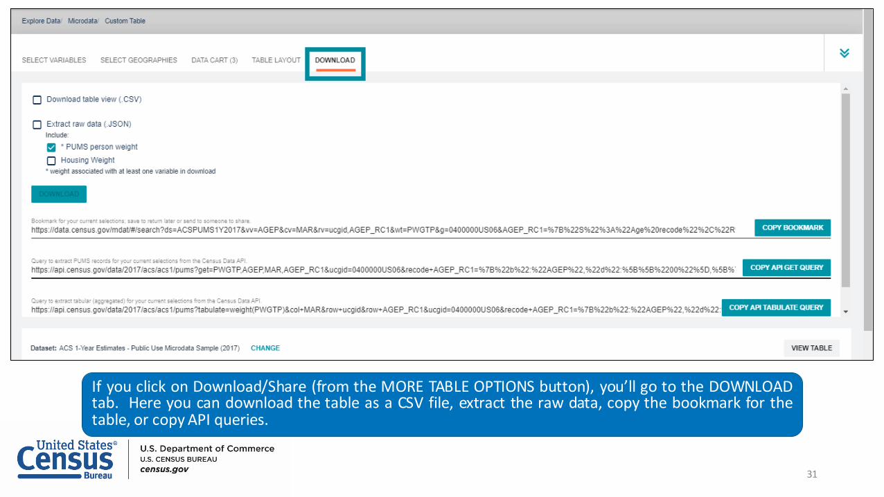
31

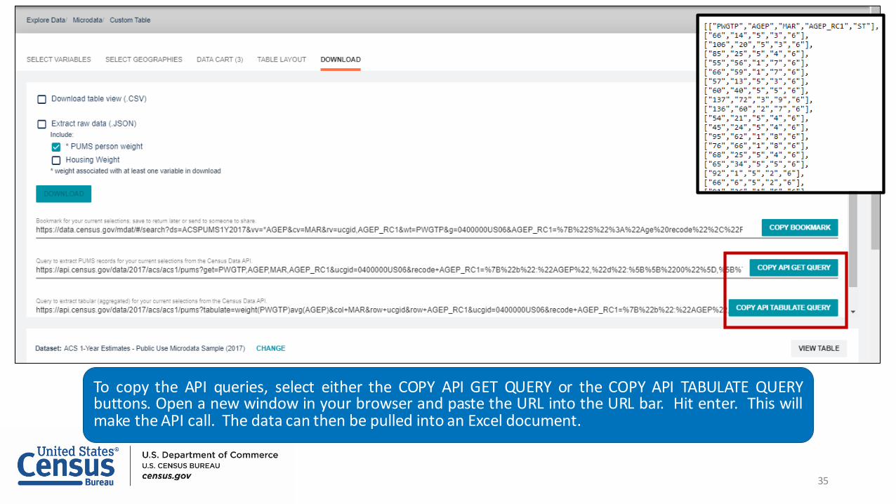
If you click on Download/Share (from the MORE TABLE OPTIONS button), you’ll go to the DOWNLOADtab. Here you can download the table as a CSV file, extract the raw data, copy the bookmark for thetable, or copy API queries.

32

Check the box next to Download table view (.CSV) to download the table as a CSV file and hit theDOWNLOAD button. Open the downloaded file. It will automatically open in Excel.

33

To extract raw data in a JSON file, check the box next to Extract raw data (.JSON). Be sure that theweight files you would like are also selected. Then hit the DOWNLOAD button. It may take a fewmoments for the JSON file to be produced. Once it has finished downloading, open it.

34

To copy the bookmark, select the COPY BOOKMARK button. Open a new window in your browser andpaste the URL into the URL bar. Hit enter. It may initially look as though it has taken you to the landingpage for Microdata Access. However, if you wait a few seconds, it will automatically open the CustomTable pane that is shown on page 24.

35

To copy the API queries, select either the COPY API GET QUERY or the COPY API TABULATE QUERYbuttons. Open a new window in your browser and paste the URL into the URL bar. Hit enter. This willmake the API call. The data can then be pulled into an Excel document.

36

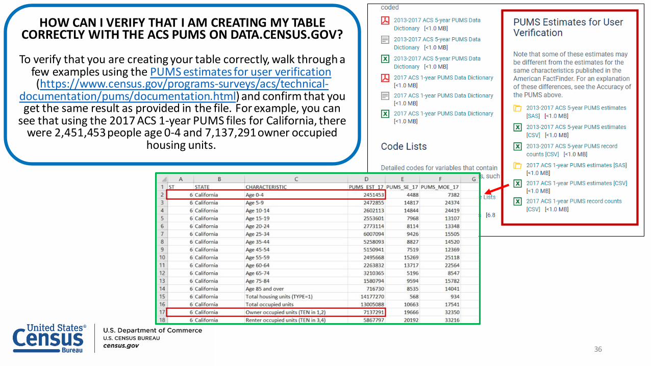
HOW CAN I VERIFY THAT I AM CREATING MY TABLE CORRECTLY WITH THE ACS PUMS ON DATA.CENSUS.GOV?

To verify that you are creating your table correctly, walk through a few examples using the PUMS estimates for user verification(https://www.census.gov/programs-surveys/acs/technical-

documentation/pums/documentation.html) and confirm that you get the same result as provided in the file. For example, you can

see that using the 2017 ACS 1-year PUMS files for California, there were 2,451,453 people age 0-4 and 7,137,291 owner occupied

housing units.

37

As discussed on a page 18, the site offers two ways to create custom groups of continuous variables. You can manually specify each grouping or you can use the Auto Group feature.

The next few pages provide directions for manually specifying your groupings.

Manually Specifying a Custom Group

38

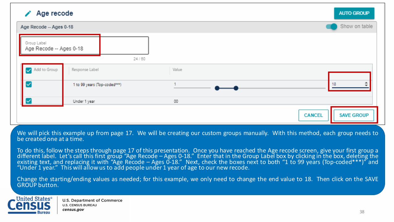
We will pick this example up from page 17. We will be creating our custom groups manually. With this method, each group needs tobe created one at a time.

To do this, follow the steps through page 17 of this presentation. Once you have reached the Age recode screen, give your first group adifferent label. Let’s call this first group “Age Recode – Ages 0-18.” Enter that in the Group Label box by clicking in the box, deleting theexisting text, and replacing it with “Age Recode – Ages 0-18.” Next, check the boxes next to both “1 to 99 years (Top-coded***)” and“Under 1 year.” This will allow us to add people under 1 year of age to our new recode.

Change the starting/ending values as needed; for this example, we only need to change the end value to 18. Then click on the SAVEGROUP button.

39

Now you’ll notice that you have your new age group of Ages 0-18 and a group with the remaining ages. The values for yournew age group are displayed as “1:18, 00.” This signifies that people aged 1 to 18 years are included in this groups, as well aspeople aged 00 (under 1 year).

To add an additional age group, select the EDIT GROUP button for the “Not Elsewhere Classified” group.

40

Like you did before, change the Group Label to something that distinguishes it from the other groups, check the box next to“Between 19 and 99,” change the starting/ending range as needed, and click on SAVE GROUP. For this example, we’ll createa recode group for people ages 19-64.

NOTE: You can not have any ages that overlap between multiple groups. For example, the tool will not allow you to create agroup for people ages 0 to 18 and another group for people ages 17-64. This is not allowed because you are trying toinclude 17 and 18 year olds in more than one group.

41

Now you’ll see that you have three different groupings listed: one for Ages 0-18, another for Ages 19-64, and the last one forpeople ages 65-99 (still named “Not Elsewhere Classified”). Let’s click on the EDIT GROUP button to change this last label.

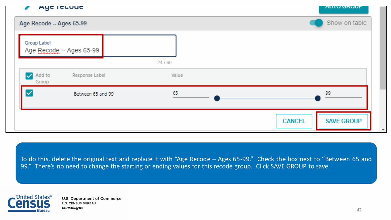
42

To do this, delete the original text and replace it with “Age Recode – Ages 65-99.” Check the box next to “Between 65 and99.” There’s no need to change the starting or ending values for this recode group. Click SAVE GROUP to save.

43

Now you have all three custom groups that you manually specified.

From here, you can continue with the steps found on page 20 of this document.

Questions?cedsci.feedback@census.gov

44