using laplace transforms for circuit analysis - github pages · consider the -domain glc parallel...

04/02/2018 circuit_analysis

http://localhost:8890/nbconvert/html/dev/EG-247-Resources/week3/circuit_analysis.ipynb?download=false 1/19

In [ ]:

% Matlab setup clear all cd matlab pwd

Using Laplace Transforms for Circuit Analysis

First Hour's AgendaWe look at applications of the Laplace Transform for

Circuit transformation from Time to Complex Frequency

Complex impedance

Complex admittance

Circuit Transformation from Time to Complex Frequency

Resistive Network - Time Domain



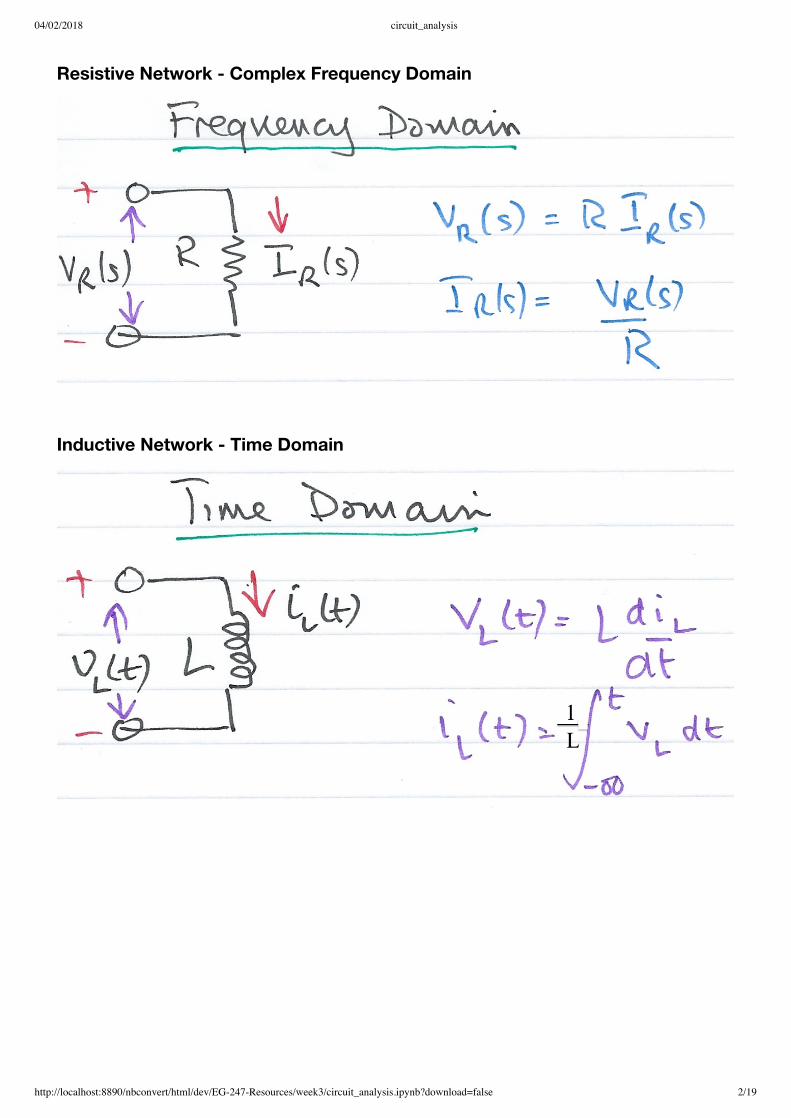
Resistive Network - Complex Frequency Domain

Inductive Network - Time Domain



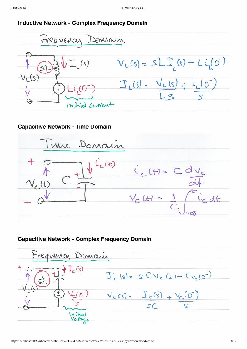
Inductive Network - Complex Frequency Domain

Capacitive Network - Time Domain

Capacitive Network - Complex Frequency Domain



Examples

Example 1

Use the Laplace transform method and apply Kirchoff's Current Law (KCL) to find the voltage acrossthe capacitor for the circuit below given that V.

(t)vc( ) = 6vc 0−



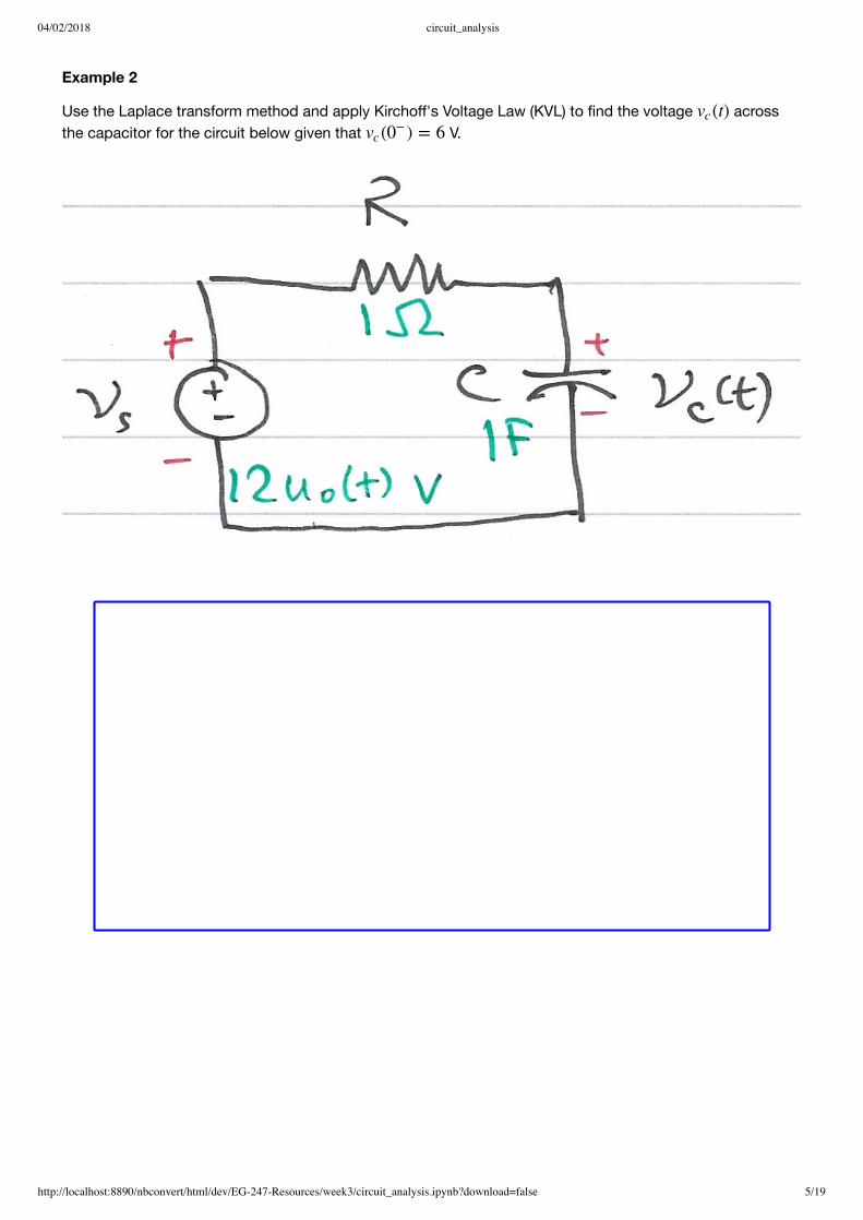
Example 2

Use the Laplace transform method and apply Kirchoff's Voltage Law (KVL) to find the voltage acrossthe capacitor for the circuit below given that V.

(t)vc( ) = 6vc 0−



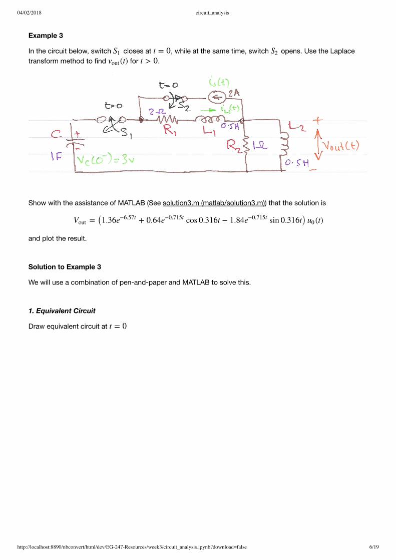
Example 3

In the circuit below, switch closes at , while at the same time, switch opens. Use the Laplacetransform method to find for .

Show with the assistance of MATLAB (See solution3.m (matlab/solution3.m)) that the solution is

and plot the result.

Solution to Example 3

We will use a combination of pen-and-paper and MATLAB to solve this.

1. Equivalent Circuit

Draw equivalent circuit at

S1 t = 0 S2(t)vout t > 0

= (1.36 + 0.64 cos 0.316t − 1.84 sin 0.316t) (t)Vout e−6.57t e−0.715t e−0.715t u0

t = 0

http://localhost:8890/nbconvert/html/dev/EG-247-Resources/week3/matlab/solution3.m



2. Transform model

Convert to transforms



3. Determine equation

Determine equation for .(s)Vout



4. Complete solution in MATLAB

In the lecture we showed that after simplification for Example 3

We will use MATLAB to factorize the denominator of the equation into a linear and a quadratic factor.

Find roots of Denominator D(s)

In [2]:

r = roots([1, 8, 10, 4])

Find quadratic form

=Vout

2s(s + 3)

+ 8 + 10s + 4s3 s2

D(s)

r = -6.5708 + 0.0000i -0.7146 + 0.3132i -0.7146 - 0.3132i



In [3]:

syms s t y = expand((s - r(2))*(s - r(3)))

Simplify coefficients of s

In [4]:

y = sym2poly(y)

Complete the Square

Plot result

y = s^2 + (804595903579775*s)/562949953421312 + 3086772113315577969665007046981/5070602400912917605986812821504

y = 1.0000 1.4292 0.6088



In [5]:

t=0:0.01:10; Vout = 1.36.*exp(r(1).*t)+0.64.*exp(real(r(2)).*t).*cos(imag(r(2)).*t)-1.84.*exp(real(r(3)).*t).*sin(-imag(r(3)).*t); plot(t, Vout); grid title('Plot of Vout(t) for the circuit of Example 3') ylabel('Vout(t) V'),xlabel('Time t s')

Worked Solution: Example 3

File Pencast: example3.pdf (worked%20examples/example3.pdf) - Download and open in Adobe AccrobatReader.

The attached "PenCast" works through the solution to Example 3 by hand. It's quite a complex, error-prone(as you will see!) calculation that needs careful attention to detail. This in itself gives justification to my beliefthat you should use computers wherever possible.

Please note, the PenCast takes around 39 minutes (I said it was a complex calculation) but you can fastforward and replay any part of it.

Alternative solution using transfer functions

http://localhost:8890/nbconvert/html/dev/EG-247-Resources/week3/worked%20examples/example3.pdf



In [6]:

Vout = tf(2*conv([1, 0],[1, 3]),[1, 8, 10, 4])

In [7]:

impulse(Vout)

Complex Impedance Z(s)Consider the -domain RLC series circuit, wehere the initial conditions are assumed to be zero.s

Vout = 2 s^2 + 6 s ---------------------- s^3 + 8 s^2 + 10 s + 4 Continuous-time transfer function.



For this circuit, the sum

represents that total opposition to current flow. Then,

and defining the ratio as , we obtain

The -domain current can be found from

where

Since is a complex number, is also complex and is known as the complex input impedanceof this RLC series circuit.

ExerciseUse the previous result to give an expression for

R + sL +1

sC

I(s) =(s)Vs

R + sL + 1/(sC)

(s)/I(s)Vs Z(s)

Z(s) = = R + sL +(s)Vs

I(s)

1

sC

s I(s)

I(s) =(s)Vs

Z(s)

Z(s) = R + sL + .1

sC

s = σ + jω Z(s)

(s)Vc



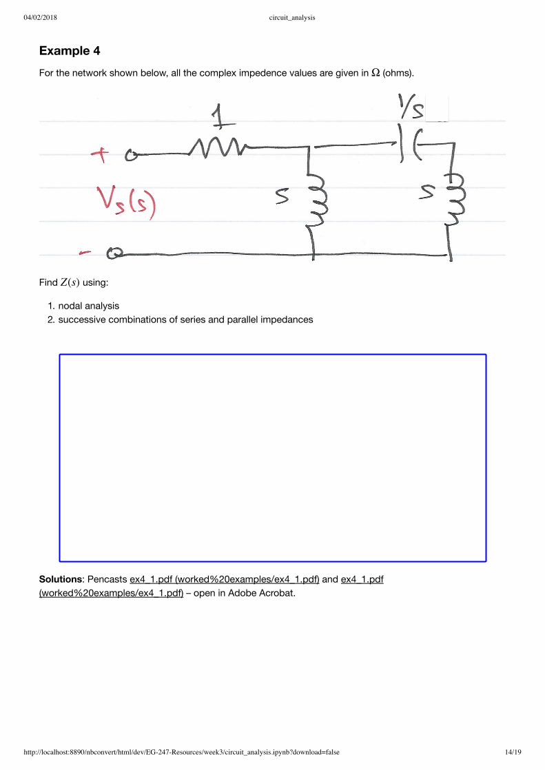
Example 4For the network shown below, all the complex impedence values are given in (ohms).

Find using:

1. nodal analysis2. successive combinations of series and parallel impedances

Solutions: Pencasts ex4_1.pdf (worked%20examples/ex4_1.pdf) and ex4_1.pdf(worked%20examples/ex4_1.pdf) – open in Adobe Acrobat.

Ω

Z(s)

http://localhost:8890/nbconvert/html/dev/EG-247-Resources/week3/worked%20examples/ex4_1.pdf

http://localhost:8890/nbconvert/html/dev/EG-247-Resources/week3/worked%20examples/ex4_1.pdf



Complex Admittance Y(s)Consider the -domain GLC parallel circuit shown below where the initial conditions are zero.

For this circuit

Defining the ratio as we obtain

The -domain voltage can be found from

where

is complex and is known as the complex input admittance of this GLC parallel circuit.

s

GV(s) + V(s) + sCV(s) = (s)1

sLIs

(G + + sC)V(s) = (s)1

sLIs

(s)/V(s)Is Y(s)

Y(s) = = G + + sC =(s)Is

V(s)

1

sL

1

Z(s)

s V(s)

V(s) =(s)Is

Y(s)

Y(s) = G + + sC.1

sL

Y(s)



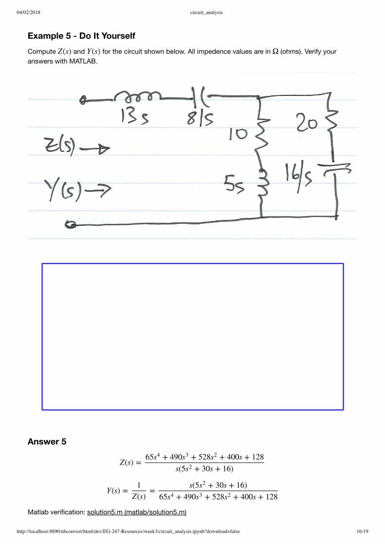
Example 5 - Do It YourselfCompute and for the circuit shown below. All impedence values are in (ohms). Verify youranswers with MATLAB.

Answer 5

Matlab verification: solution5.m (matlab/solution5.m)

Z(s) Y(s) Ω

Z(s) =65 + 490 + 528 + 400s + 128s4 s3 s2

s(5 + 30s + 16)s2

Y(s) = =1

Z(s)

s(5 + 30s + 16)s2

65 + 490 + 528 + 400s + 128s4 s3 s2

http://localhost:8890/nbconvert/html/dev/EG-247-Resources/week3/matlab/solution5.m



Example 5: Verification of Solution

In [8]:

syms s;

z1 = 13*s + 8/s; z2 = 5*s + 10; z3 = 20 + 16/s;

In [9]:

z = z1 + z2 * z3 /(z2 + z3)

In [10]:

z10 = simplify(z)

In [11]:

pretty(z10)

Admittance

In [12]:

y10 = 1/z10; pretty(y10)

z = 13*s + 8/s + ((5*s + 10)*(16/s + 20))/(5*s + 16/s + 30)

z10 = (65*s^4 + 490*s^3 + 528*s^2 + 400*s + 128)/(s*(5*s^2 + 30*s + 16))

4 3 2 65 s + 490 s + 528 s + 400 s + 128 ------------------------------------- 2 s (5 s + 30 s + 16)

2 s (5 s + 30 s + 16) ------------------------------------- 4 3 2 65 s + 490 s + 528 s + 400 s + 128

using laplace transforms for circuit analysis - github pages · consider the -domain glc parallel...

Documents