using hydrological tracers to study pesticide fate and ... · using hydrological tracers to study...

Using Hydrological tracers to

Study Pesticide Fate and

Transport on an Agricultural

Field

Brian Joseph Sweeney

Institute for Hydrology

University of Freiburg, Germany

Advisor: Prof. Dr. Jens Lange

Co-advisor: Dr. Gwenael Imfeld

A thesis submitted for the degree of

Master of Science

under the direction of Prof. Dr. Jens Lange

Freiburg i. Br., November 2012

mailto:[email protected]

http://www.hydro.uni-freiburg.de/

http://www.uni-freiburg.de/

Abstract

Non-point source pollution from pesticide leaching and runoff has become and im-

portant environmental problem. In a study by Winchester et al. (2009) detectable

levels of pesticides were found in 87 % of drinking water samples in 12 of the corn

belt states. This study focuses on the assessment of dye tracers as surrogates for S-

metolachlor fate and transport in the end that they be used as a possible low cost

substitutes in S-metolachlor risk studies. Two experiments were performed in order to

evaluate the dyes. In the first, dyes and pesticides were applied concurrently, along

with sodium bromide as a conservative tracer, to the soil surface of a 5 x 15 m area and

left under prevailing meteorological conditions. The progression of each constituent

was monitored in surface soils and subsequent runoff events. Nominal recoveries were

reported in collected runoff samples totaling 0.4, 0.06, and 0.14 % for Br-, UR and

SRB. This experiment was performed from April-July, 2012 in Alteckendorf, France.

After 90 days soil cores samples were extracted from the site and analyzed for tracer

and pesticide residues to determine leaching depths and persistence. Approximately

87 % of Bromide was recovered in soil cores taken to a depth of 1 m on the 12th fo

July. Wavelength shifting of dye tracers in soil samples after the 26th of June masked

fluorescence analysis such that their quantification could not be made after this date.

S-metolachlor analysis of water and soil samples was yet to be performed at the time

of conception of this document.

In the second experiment dye and bromide tracer leaching under high intensity

rainfall conditions was executed on a 2 x 4.8 m plot. Simulated rainfall equipment was

used to produce rainfalls approximately equal to a two year storm for the catchment.

Pesticides were not included in this study as a means of reducing pollution and obtained

values were compared to results from similar studies of S-metolachlor leaching as a

means of validation. All tracers were found in measurable amounts in tile drain effluent

after ± 60 mm of applied rainfall, pointing to preferential flows to field tile drains.

Keywords: Multi-tracer, S-metolachlor, fate, transport, surrogate

Zusammenfassung

Der diffuse Pestizidtransport von Ackern zu Oberflachenwassern ist zu einem wichti-

gen Umweltproblem geworden. In einer Studie von Winchester et al. (2009) wurden

nachweisbare Konzentrationen von Pestiziden in 87 % aller Trinkwasserproben in 12

US-Bundesstaaten gefunden. Ziel dieser Arbeit ist es zu untersuchen, inwiefern Farb-

stofftracer als Ersatzstoffe fur die Untersuchung von Pestizidverbleib und -transport

verwendbar sind. Dafur wurden zwei Experimente durchgefuhrt. Im ersten Exper-

iment wurden zwei Farbstofftracer (Uranin und Sulforhodamin B) gemeinsam mit

Pestiziden und einem konservativen Tracer (Bromid) auf den Boden einer 5 x 15 m

großen Flache unter am Standort vorherrschenden meteorologischen Bedingungen aus-

gebracht. Bromid wurde verwendet, um den Abbau und die Ausbreitung der Farb-

stoffe und der Pestizide nachzuvollziehen. Die Ausbreitung jedes Stoffes wurde mit-

tels Proben aus oberflachennahem Boden und oberirdischem Abfluss gemessen. Die

Wiederfindung der Tracer in Abflussproben war 0.4, 0.06, und 0.14 % fur Br-, UR und

SRB. Dieses Experiment wurde von April bis Juli 2012 in Alteckendorf im Frankre-

ich durchgefuhrt. 90 Tage nach der Ausbringung der Stoffe wurden Bodenproben aus

dem Versuchsgebiet entnommen und auf Farbstofftracer- und Pestizidruckstande un-

tersucht, um Auswaschungstiefen und Persistenz jedes Stoffes zu bestimmen. Ungefar

87 % des Bromids wurden in Bodenproben aus 1 m Tiefe am 12.7.2012 wiedergefun-

den. Eine Verschiebung der Fluoreszenz-Wellenlange des Farbstofftracers am 26. Juni

hat die Analyse verhindert und es wurden keine Messungen mehr nach diesem Datum

gemacht. Die S-Metolachlor Analyse war bei der Fertigstellung dieser Dokuments noch

nicht durchgefuhrt worden.

Im zweiten Experiment wurde die Farbstoff- und Bromid-Tracerversickerung auf

einer 2 x 4.8 m großen Flache bei hoher Regenintensitat gemessen. Dies entspricht ±60 mm Regen, was der Intensitat eines zweijahrigen Ereignisses gleich kommt. Mes-

sungen und Proben des oberirdischen sowie des Dranageabflusses wurden genommen

und davon wurde die Wiederfindung der Tracer kalkuliert. Diese Werte wurden mit

der Literatur verglichen, da keine Pestizide appliziert wurden. Alle Tracer wurden im

Dranageabflussen gemessen.

To Ma and Pa

Acknowledgements

I would like to acknowledge the help of Jens Lange and Barbra Herbstritt

from the Freiburg team in there assistance towards the completion of the

project and the conception of this document. I would also like to thank all

the help from the Strasbourg team; Gwenael Imfeld, Sylvain Payraudeau,

Marie Lefrancq, Benoit Guyot, Diogo, Eric and the whole lot, for their

support in the field and ideas in the hall.

Contents

List of Figures vii

List of Tables ix

List of Abbreviations & Symbols xi

1 Introduction - Literature Search 1

2 Aims of the project 7

2.1 Final aim . . . . . . . . . . . . . . . . . . . . . . . . . . . . . . . . . . . 7

2.1.1 Aims of Plot Experiment . . . . . . . . . . . . . . . . . . . . . . 7

2.1.2 Aims of Tile drain Experiment . . . . . . . . . . . . . . . . . . . 8

3 Materials & Methods 9

3.1 Study site . . . . . . . . . . . . . . . . . . . . . . . . . . . . . . . . . . . 9

3.1.1 Site description and climate . . . . . . . . . . . . . . . . . . . . . 10

3.1.2 Plot measurement devices . . . . . . . . . . . . . . . . . . . . . . 12

3.1.3 Catchment measurement devices . . . . . . . . . . . . . . . . . . 12

3.1.4 Field sampling . . . . . . . . . . . . . . . . . . . . . . . . . . . . 14

3.2 Tile Drain Experiment . . . . . . . . . . . . . . . . . . . . . . . . . . . . 15

3.2.1 Site description . . . . . . . . . . . . . . . . . . . . . . . . . . . . 16

3.2.2 Simulated rain equipment . . . . . . . . . . . . . . . . . . . . . . 16

3.2.3 Measurement devices and Sampling . . . . . . . . . . . . . . . . 18

3.3 Analysis of Water Samples . . . . . . . . . . . . . . . . . . . . . . . . . . 18

3.3.1 Bromide tracer analysis . . . . . . . . . . . . . . . . . . . . . . . 19

3.3.2 Fluorescent tracer analysis . . . . . . . . . . . . . . . . . . . . . 19

3.3.3 Hydrochemistry testing . . . . . . . . . . . . . . . . . . . . . . . 20

iii

CONTENTS

3.4 Analysis of Soil Samples . . . . . . . . . . . . . . . . . . . . . . . . . . . 20

3.4.1 Soil pH . . . . . . . . . . . . . . . . . . . . . . . . . . . . . . . . 20

3.4.2 Bulk Density and Field Moisture Content . . . . . . . . . . . . . 21

3.4.3 Carbonaceous Material . . . . . . . . . . . . . . . . . . . . . . . 21

3.4.4 Particle size . . . . . . . . . . . . . . . . . . . . . . . . . . . . . . 22

3.4.5 Saturated hydraulic conductivity . . . . . . . . . . . . . . . . . . 22

3.4.6 Soil Moisture Retention Curve . . . . . . . . . . . . . . . . . . . 23

3.4.7 Bromide Tracer - Desorption from soil and analysis . . . . . . . . 23

3.4.8 Fluorescent tracers - desorption from soil and analysis . . . . . . 24

3.5 Sorption Experiment . . . . . . . . . . . . . . . . . . . . . . . . . . . . . 24

3.5.1 Batch sorption tests . . . . . . . . . . . . . . . . . . . . . . . . . 24

3.5.2 Sorption Isotherms . . . . . . . . . . . . . . . . . . . . . . . . . . 26

4 Results 29

4.1 Plot Campaign . . . . . . . . . . . . . . . . . . . . . . . . . . . . . . . . 29

4.1.1 Plot Water Samples . . . . . . . . . . . . . . . . . . . . . . . . . 29

4.1.2 Soil Samples . . . . . . . . . . . . . . . . . . . . . . . . . . . . . 30

4.1.2.1 Soil Samples April - July . . . . . . . . . . . . . . . . . 32

4.1.2.2 Core Samples . . . . . . . . . . . . . . . . . . . . . . . . 34


4.2.1 Simulated Rain Equipment . . . . . . . . . . . . . . . . . . . . . 38

4.2.2 Tracer Breakthrough Curves . . . . . . . . . . . . . . . . . . . . 40

4.2.3 Tracer Mass Balance . . . . . . . . . . . . . . . . . . . . . . . . . 41

4.3 Batch Sorption Experiment . . . . . . . . . . . . . . . . . . . . . . . . . 43

5 Discussion 47

5.1 Plot Water Samples . . . . . . . . . . . . . . . . . . . . . . . . . . . . . 47

5.2 Plot Soil Samples . . . . . . . . . . . . . . . . . . . . . . . . . . . . . . . 49


5.4 Batch Sorption Experiment . . . . . . . . . . . . . . . . . . . . . . . . . 53

6 Conclusion 55

References 57

iv

CONTENTS

A Supplementary Figures 63

B Supplementary Tables 67

v

List of Figures

3.1 Pedology map of Alteckendorf . . . . . . . . . . . . . . . . . . . . . . . . 11

3.2 Climate graph of Alteckendorf, France . . . . . . . . . . . . . . . . . . . 11

3.3 Map of measurement devices at the experimental plot . . . . . . . . . . 13

3.4 Placement of extracted core samples . . . . . . . . . . . . . . . . . . . . 15

3.5 Site of tile drain experiment . . . . . . . . . . . . . . . . . . . . . . . . . 16

3.6 Diagram of simulated rain device . . . . . . . . . . . . . . . . . . . . . . 17

4.1 Normalized tracer concentrations and suspended solids flux . . . . . . . 31

4.2 Nitrate and sulfate from April-July, 2012 . . . . . . . . . . . . . . . . . . 32

4.3 Bromide, chloride, UR, and SRB from April-July, 2012 . . . . . . . . . . 33

4.4 VWC and pH development from April-July 2012 . . . . . . . . . . . . . 34

4.5 Bromide, chloride, nitrate, and sulfate with depth: 12th, July 2012 . . . 35

4.6 CEC, pH, and GWC; July 12th, 2012 . . . . . . . . . . . . . . . . . . . 37

4.7 Histogram of rainfall events at Waltenheim . . . . . . . . . . . . . . . . 38

4.8 Precipitation event recurrence intervals . . . . . . . . . . . . . . . . . . . 39

4.9 Distribution of simulated rain equipment . . . . . . . . . . . . . . . . . . 40

4.10 Tile drain experiment tracer BTCs w/ recovery rates and normalized

anion conc. . . . . . . . . . . . . . . . . . . . . . . . . . . . . . . . . . . 42

4.11 Comparison of tracer BTCs in drain effluent . . . . . . . . . . . . . . . . 43

4.12 UR and SRB Sorption Isotherms . . . . . . . . . . . . . . . . . . . . . . 45

A.1 UR and SRB Fluorescence spectroscopy calibration curves . . . . . . . . 63

A.2 Background fluorescence increases from high water tape . . . . . . . . . 64

A.3 Soil moisture curves . . . . . . . . . . . . . . . . . . . . . . . . . . . . . 64

A.4 Langmuir and Freundlich linearizations . . . . . . . . . . . . . . . . . . 65

vii

List of Tables

3.1 Chemical properties of used tracers and pesticides . . . . . . . . . . . . 10

3.2 Kd, Koc, and half-lives of dye tracers and S-metolachlor . . . . . . . . . 10

3.3 Equipment installed during the plot experiment Alteckendorf, France. . 12

3.4 Equipment found at the catchment and drain outlets, evaluated param-

eter and type of measurement performed. . . . . . . . . . . . . . . . . . 13

4.1 Estimated tracer recovery rates for rain event of 2nd of May, 2012 at

Alteckendorf, France . . . . . . . . . . . . . . . . . . . . . . . . . . . . . 30

4.2 Bromide tracer recovery from the soil column for soil cores extracted on

12.7.2012 . . . . . . . . . . . . . . . . . . . . . . . . . . . . . . . . . . . 36

4.3 Distribution statistics of simulated rain equipment . . . . . . . . . . . . 39

4.4 Tracer mass balances for measured parameters . . . . . . . . . . . . . . 41

4.5 Langmuir and Freundlich isotherm coefficients w/ R2 and RMSE . . . . 44

4.6 Distribution coefficient (Kd) [cm3/g] obtained from batch study of UR

and SRB at 8 different concentrations . . . . . . . . . . . . . . . . . . . 44

B.1 Product information of used tracing elements . . . . . . . . . . . . . . . 67

B.2 Plot water sample sediment flux and tracer concentrations . . . . . . . . 67

B.3 Mass balance calculations of tracers in soil surface samples . . . . . . . . 67

B.4 Saturated hydraulic conductivity (Ks) from site characterization . . . . 68

B.5 Correlation matrices (Pearson and Spearman) of water sample constituents 68

B.6 Correlation matrices (Pearson and Spearman) of soil sample constituents 69

ix

List of

Abbreviations

& Symbols

∆h Changes in water level [cm]

ψ Matric suction head in soils [-hPa or

-cm of water head]

ρsoil Bulk density of the soil [g/cm3]

ρwater Density of water at 20 ◦C [g/cm3]

A Area [cm2]

C Concentration at equilibrium [mg/L

; µg/L]

C0 Initial concentration [mg/L ; µg/L

Ka Langmuir adsorption coefficient

Kd Distribution coefficient [cm3/g]

Kd Distribution or partition coefficient

solid/water phase [cm3/g ; mL/g]

Kf Freundlich adsorption coefficient

Ks Saturated hydraulic conductivity

[cm/sec; cm/day]

l Height of sample cylinder [cm]

M Mass [g ; mg]

mdry Mass of soil sample after drying at

105 ◦C for 48 hr [g]

msample Mass of soil sample at field conditions

[g]

q Adsorbate per unit mass of adsorbent

at equilibrium [mg/g ; µg/g]

qm The maximum adsorbable value of

adsorbate per unit mass of absorbent

[mg/g; µg/g]

t Time [sec]

V Volume [mL ; L ; m3]

Vcyl Volume of sampling cylinder [cm3]

Br- Bromide

BTC Breakthrough curve

CI Confidence interval

Cl- The chemical substance Chloride

DDW Deionized distilled water

GWC Gravimetric water content [%]

LHyGeS laboratory of hydrology and geo-

chemistry of Strasbourg

LL Langmuir linearization

NaBr Sodium Bromide salt

NLLS Nonlinear least squares regression

NO3- The chemical substance Nitrate

pF curve Soil moisture retention curve

RMSE Root mean squared error

SO4-2 The chemical substance Sulfate

SRB Fluorescent dye sulforhodamine B,

C27H29N2O7S2Na

SS Statistically significant

Stdev Standard deviation

UR Fluorescent dye uranine, C20H1205Na2,

also known under the name fluores-

cein

VWC Volumetric water content [%]

xi

1

Introduction - Literature Search

Non-point source runoff from agriculture activities is an ever increasing problem in the

pollution of our waterways and aquifers. World use of pesticides was approximately 5.2

billion pounds (2.36 billion kg.) in both 2006 and 2007 (Grube et al., 2011), with 198

million metric tonnes of fertilizer being used in 2010 (FAO, 2010). Three sets of factors

are of known importance in the fate and transport of pesticides and nutrients applied to

soils; 1) management factors , 2) hydrological factors, and 3) chemical factors (Baker,

1999).

Management factors: many agricultural management practices have been examined

for their usefulness in reducing non-point pollution from acreage such as: no till farm-

ing, also known as conservation farming(Andreini and Steenhuis, 1990; Olsen, 1995;

Watanabe et al., 2007); reduction of soil compaction by management of sowing and

harvesting times (Batey, 2009; Soane and van Ouwerkerk, 1995); alignment of rows to

reduce direct runoff (USDA, 2001); buffer strips (USDA, 2000); etc. However, due to

heterogeneity of natural conditions and the unpredictability of meteorological events

site management practices cannot stop all cases of pesticide runoff and leaching. Thus,

further management and mitigation practices, such as artificial wetlands (Lange et al.,

2011), focus on the inevitability of pollutants reaching surface waters. For terseness

further discussion has been excluded.

Hydrological factors: three main hydrological factors, the rate of infiltration, the

route of infiltration, and quantity of runoff, are the main processes responsible for

the transport of pesticides and other agrochemicals off-site (Baker, 1999; Conservation,

1993; Oliver et al., 2012). Infiltration rates are extremely site specific and dependent on

1

1. INTRODUCTION - LITERATURE SEARCH

area soil properties making ameliorations difficult or economically unfeasible. Several

management practices, such as mulching or no-till, have been shown to increase water

absorption in the top soil layer by additions of biomass (Smets et al., 2008). This,

however, does not change soil properties further down in the soil column where deep

percolation occurs and possibilities of contamination exist by way of leaching pesticides

and solutes.

Infiltration pathways are also heavily dependent on site characteristics; land usage;

crop type, stage, and cover; and tilling practices (Mohanty et al., 1996; Wainwright,

1996; Watanabe et al., 2007). Mohanty et al. (1996) reports that nearly 91% (under

corn row), 89% (under nontrafficked interrow), and 92% (under trafficked interrow) of

the saturated water flux occurs through large pores and cracks in glacial till catchments,

at water tension ranges of 0-0.3 hPa. Savabi et al. (2008) found higher earthworm

(Lumbricus terrestris) activity under no-till fields and subsequent higher infiltration

rates due to increased macroporosity. Increases in field macroporosity can lead to

contamination of shallow aquifers during large rain events by bypassing the soil matrix,

leading to deeping infiltration, and increased risk of contamination of supply wells

(Cey et al., 2009; Hrudey et al., 2003).

Runoff from agricultural fields is dependent on rainfall quantity and intensity;

farming practices; and site soil properties (Mohanty et al., 1996; Wainwright, 1996;

Watanabe et al., 2007). In some cases runoff can exceed 70% of rainfall (Watanabe et al.,

2007), with rainfall event intensity being the driving factor in the percentage of runoff

measured (Wainwright, 1996). This occurs when the rainfall rate is less than the ini-

tial infiltration rate (suction driven), of the soil, but greater than the final gravity

dominated rate, at this point water cannot be taken up by the soil profile as fast as

it is added and ponding and runoff occur (Baker, 1999). Furthermore, the mode of

pesticide transport in runoff (in the dissolved phase or in association with transported

sediment) is dependent on pesticide properties (Oliver et al., 2012). Type and quan-

tity of sediment loads also play a large role in pesticide transport (Agassi et al., 1995)

and are shown to be highly correlated to tillage practices and site soil characteristics

(Cogo et al., 1984).

Chemical properties: chemical properties that determine transport through the un-

saturated zone depend on many factors: ion exclusion; ion exchange; volatilization;

dissolution and precipitation; chemical and biological transformation; bio-degradation;

2

adsorption; diffusion; dispersion; and persistence (Tindall et al., 1999), the four most

important properties being, persistence (or resistance to transformation or degrada-

tion), soil adsorption, water solubility, and vapor pressure (volatilization) (Baker, 1999).

These properties determine the most likely transport process a chemical will take. In

the case of strongly adsorbed pesticides (e.g., with distribution coefficients (Kd) > 200),

the main mode of transport is with sediment, because pesticide is not readily released

to water flowing over or through the soil surface; whereas for moderately adsorbed

pesticides (1 < Kd < 20), pesticide is more readily released to water flowing over or

through the soil surface, and runoff losses with water dominate over losses with sediment

(Baker, 1999). Currently there is a good understanding of most transport processes of

pesticides (Flury, 1996). There has also been extensive work done on the impact of

management practices on hydrological processes in conjunction with pesticide trans-

port (Andreini and Steenhuis, 1990; Olsen, 1995; Smets et al., 2008; Watanabe et al.,

2007). However heterogeneity between sites and soils is rarely addressed and individual

studies usually cannot be transfered between sites and catchments. In most cases, site

specific testing must be completed in order to characterize high risk pollution pathways

within individual catchments. Further complications arrive, since chemical properties

of pesticides differ greatly from one to another (Hertfordshire, 2009). Moreover testing

has mainly focused on the use of lysimeters or soil cores to characterize entire catch-

ments (Fank and Harum, 1994; Vanderborght et al., 2002). This approach brings into

question the validity of the transfer of observations from the small to the large scale in

processes such as macroporosity given its heterogeneity (Bloschl and Sivapalan, 1995).

This study’s focus is to show that dye tracers can be used as a surrogate for the pesti-

cide S-metolachlor and provide a low cost alternative in the case of site characterization

while using a scale representative of the catchment as a whole.

Water tracers have been employed as a means of determining catchment hydrology

for nearly 150 years (Knop, 1878). Most tracer tests focus on their use as a method to

determine water transport and arrival times in surface and groundwaters (Davis et al.,

1980; Haggerty et al., 2008). To that end tracers have been assessed using a set of

criteria to determine if they exhibit “conservative” or “ideal” behavior (Bowman, 1984;

Flury and N.N., 2003; Smart and Laidlaw, 1977). Bowman (1984) states the criteria

for an effective soil water tracer are:

3


1. the tracer should not be significantly sorbed or otherwise retarded by the soil of

interest

2. the tracer should be exotic to the soil environment, or should be present naturally

at low concentrations

3. the tracer should be conservative in that it is not significantly degraded chemically

or biologically during the course of an experiment.

Other considerations in choosing a tracer include: ease of quantitation in a soil solution

matrix; cost of the tracing element; and the potential for adverse environmental im-

pacts, particularly important if the tracer is to be used in unconfined field studies. How-

ever, only certain processes can be studied from conservative tracers such as, advection,

dispersion (spreading of break through curves), and transient storage or mass transfer

(tailing in break through curves) (Fank and Harum, 1994; Sanchez-Vila and Carrera,

2004).

Dye tracers have seen use as surrogates for pesticide fate and transport for up-

wards of 20 years. A surrogate is defined in environmental microbiology as an organ-

ism, particle, or substance used to study the fate of a pathogen in a specific envi-

ronment (Sinclair et al., 2012). Uranine and rhodamine WT dye tracers have already

been employed in laboratory column experiments designed to evaluate the dyes as ad-

sorbing tracers that mimic pesticide adsorption (Sabatini and Austin, 1991). In the

study Sabatini demonstrates that the tracers were able to delimit the break through

of atrazine and alachlor in column experiments, with the BTC peak of uranine com-

ing before and sulforhodamine B after the pesticides. Vanderborght et al. (2002) used

brilliant blue and sulforhodamine B dyes to assess solute transport mechanisms in

soil cores and Sinreich et al. (2007) used uranine and sulfrhodamine B as conserva-

tive and sorbing tracers respectively, in a comparative tracer test where both tracers

passed through a thin soil layer before entry into a karst system. Most studies to date

focus on the sorption properties of dyes and pesticides and the use of dyes as delim-

iters or indicators of pesticide leaching (Sabatini and Austin, 1991; Vanderborght et al.,

2002). These works focus on pesticide and dye leaching, most commonly in associa-

tion with preferential flows, during heavy rainfalls directly or shortly after application

(Andreini and Steenhuis, 1990; Vanderborght et al., 2002). Very little work has been

done on pesticide or dye tracer fate and transport under field conditions. Cornoi et al.

4

(2011) studied the fate of S-metolachlor under field conditions, but focused primarily

on pesticide leaching over time. More understanding of the processes effecting pesti-

cide dissipation in the top layer of soil need to be developed in order to better contain

pollution. This is also reflected in the large range of half-life values of S-metolachlor

in photodegradation studies, which range from 6.83 - 94.95 days (Costello and Hetrick,

2008); the use of organic matter and acetone as a photosensitizer being cited for the

large range of values. No previous work was found in which the sorption and degrada-

tion of dyes at normal field conditions was used as a means of delimiting or determining

pesticide fate.

The pesticide of focus in this study is S-metolachlor, which is shown to be moder-

ately adsorbed, have a high water solubility and a low rate of volatilization (Bowman,

1990; Hertfordshire, 2009; University, 1993). It has been widely used for selected weed

control for over 30 years and normally applied preemergence. The mean half life of

S-metolachlor was demonstrated to be 23 days in dissipation studies at different Eu-

ropean field sites (OConnell et al., 1998); where S-metolachlor persistence was shown

to be correlated to the application amount, since higher application amounts increased

leaching to depths were photo- and aerobic degradation were reduced (Cornoi et al.,

2011). Monitoring of S-metolachlor in runoff and tile drain effluent was performed by

Gaynor et al. (2002) in which 91% of total accounted pesticide loss was through the tile

drainage system, with 92% being transported in the first event after herbicide applica-

tion. Gish et al. (2009) reported volitalization losses of metolachlor as 19.3 - 11.4 % of

applied mass for a period of 3 days after pesticide application, the larger volitization

losses coming from plots with higher soil moisture contents. As before stated, there are

large differences in estimations of S-metolachlor persistence with in field half-life val-

ues ranging from 11-31 days in European studies (Hertfordshire, 2009) to 6.83 - 94.95

days in American studies (Costello and Hetrick, 2008), which displays either the site

specifity or conditional dependence of S-metolachlor decay.

Simulated rainfall experiments have successfully used to evaluate runoff and sed-

iment transport from agricultural fields for many years (Grace and Eagleson, 1966;

Sangesa et al., 2010; Touma and Alberge1, 1992; Wainwright, 1996). Many studies

have used simulated rainfall as a means of determining solute leaching rates during

5


large or high intensity events (Flury, 1996). Kung et al. (2000) tested deep leaching

of adsorbing and non-adsorbing tracers to determine transport processes involved in

leaching to field tile drains. Most rainfall simulations provide intensities well above

extreme events, such as discussed in Agassi and Bradford (1999) and Dunkerley (2008)

and reproduce inadequately natural rainfall. In reproducing natural rainfall the follow-

ing must be considered: drop size; drop impact kinetics; uniform rainfall intensity and

random drop size distribution; uniform rainfall application over the desired area; ver-

tical angle of impact; and natural occurrence of simulated event size (Blanquies et al.,

2003). The simulated rain experiment, in the case of this study, was performed to

study the mass recovery of dye tracers in rain events within 24 hours after applica-

tion; given that most S-metolachlor leaching is shown to occur in the first rain event

(Gaynor et al., 2002) and that pesticide leachate mass is inversely proportional to the

time elapsed between application and the first infiltration event (Flury, 1996). In this

way, the behavior of the fluorescent dyes under certain meteorological conditions could

be assessed that did not occur during the plot experiment.

It is believed that dye tracers can be effectively used as surrogates for the fate and

transport of S-metolachlor under field conditions. While it is doubtful that dyes can

mimic pesticide behavior completely, such that driving processes demonstrate a correla-

tion of 100 %, it is thought that they can provide a rough estimation of these processes.

It is also believed that dyes can be used as an ”early warning system” or ”delimiter” of

pesticide peaks in catchment effluent, such as been shown in laboratory column experi-

ments by Sabatini and Austin (1991). In this way, dye tracers that have already found

use in the determination of pesticide overspray during application (Barber and Parkin,

2003) could be further monitored to delineate pesticide peaks from runoff and leaching

to surface waters before they negatively impact water quality.

6

2

Aims of the project

2.1 Final aim

This study’s goal is to assess the use of two dye tracers as surrogates in quantifying

S-metolachlor fate and transport at the plot scale and determine their viability as such.

Two experiments were performed under different conditions in order to better define

individual transport processes; the aims of each are discussed below. Results from plot

scale experiments are then to be applied at the catchment scale to make inferences

towards driving transport processes within the catchment and the risk of pollution

posed by each.

2.1.1 Aims of Plot Experiment

The plot experiment has the aims of:

• Establishing an event based mass balance for tracers (Bromide, Uranine, Sul-

forhodamine B) and S-metolachlor.

• Investigating the hydrological processes of sediment deposition, runoff, and infil-

tration, at the soil surface and in the soil column.

• Understanding sorptive properties of site soils for assessment of retention and

retardation of S-metolachlor and tracers.

• Understanding the decay and transport processes of tracers compared to S-Metolachlor

and their link to prevailing hydro-chemical and meteorological conditions.

7

2. AIMS OF THE PROJECT

The plot experiment was carried out under prevailing meteorological conditions as

a means to better evaluate the dynamic processes of a normal spring-summer season.

2.1.2 Aims of Tile drain Experiment

The goal of the tile drain experiment is to quantify individual solute transport processes,

(runoff, infiltration, and macropore flow) under high rainfall conditions. This shall be

performed through the evaluation of the following points:

• Calculation of tracer mass balances under high rainfall conditions.

• Assessment of initial and final conditions and their impact on solute transport

through the soil column to the tile drain.

• Quantification of a processes’ contribution to solute transport.

The plot experiment utilized a simulated rainfall system with application rates

similar to an extreme two year event, in order to recreate the desired meteorological

conditions.

8

3

Materials & Methods

3.1 Study site

The study catchment Katzenlauf is located at 8 ◦51’44.136”E, 21 ◦53’14.189”N close to

the village of Alteckendorf, France. The chosen plot area measured approximately 5 m

x 15 m and was located circa 100m from the upper boundary of the catchment area

in order to reduce possible downstream effects. Plot width was chosen based on the

pesticide application method (sprayer boom of 6 m length), and plot length was chosen

to reduce plot asymmetry. Crops planted inside of the plot area consisted of sugar beet

(Beta Vulgaris) with the total crop makeup of the catchment comprising of 68% corn,

16% wheat 4% sugar beet (2% fallow). A slow release fertilizer was applied to the field

at the end of March with pesticides and tracers being applied several weeks later on the

same day in April, 2012 (exact dates are excluded for the privacy of the farmer). This

was done in the interest of facilitating mass balance calculations of tracer and pesticide

development over time.

900 g of uranine and sulforhodamine B along with 4.5 kg of sodium bromide (NaBr)

were mixed with 30 liters of water and applied to the soil surface using a backpack

sprayer. Care was taken to apply the tracers in a homogeneous manner as possible.

An effort was also made to reduce the amount of soil compaction by distributing the

sprayer’s weight over a larger area and limiting the number of footfalls on the plot

surface. Only the free anion bromide Br- was analyzed, making the measurable amount

of tracer equal to approximately 3.5 kg. The chemical properties of tracers are shown

in table 3.1 and product information in appendix table B.1. Table 3.2 gives literature

9

3. MATERIALS & METHODS

values of Distribution coefficient (Kd), normalized Kd to soil organic fraction value

(Koc), half-life (DT50) photostability, hydrolytic stability half-life, and half-life in soils,

for dye tracers and S-metolachlor. Tracer masses were chosen in consideration of the

photodegradation rate of uranine and the detection limits of all tracing elements in soil

and water samples. Masses per m2 were 11.64 g/m2 for dye tracers and 45.21 g/m2

for Br-.

Table 3.1: Chemical properties of tracers and pesticides used in experiments at Alteck-endorf, France for experiments from April-July, 2012.

Chemical Molecular FormulaMolecular

WeightpKa log Kow Solubility in H20

Excit/EmitWavelength

Sulforhodamine Ba C27H29N2O7S2Na 580.65 < 1.5 -2.02 70 g/L 565/590

Uraninea C20H1205Na2 376.15 5.1 -1.33 25 g/L 490/520

Sodium Bromideb NaBr 102.91 909 g/L —

Metalochlorc C15H22ClNO2 283.79 3.05 0.864 g/L 266/274Values determined from: a)Kasnavia et al. (1999) b)Roth Chemicals (2011) c)Commission (2004)

Table 3.2: Distribution coefficient (Kd), normalized Kd to soil organic fraction value(Koc), half-life (DT50) photostability, hydrolytic stability half-life, and half-life in soils; forUR, SRB and S-metolachlor.

Constituent Kd [cm3/g] Koc [cm3/g] Photostability water DT50 Hydrolytic stability DT50 Soil DT50

UR 0 − 0.31a dependent on focb pH dependentd stableb —

SRB 1.9 − 3.2b dependent on focb Initial Conc. Dependente stableb —

S-metolachlor 1.3 − 55.8c 110 − 369c 6 − 12dc stablec 11 − 31dc

a)Hadi et al. (1997) b)Sabatini (2000) c)Commission (2004) d)Smith and Pretorius (2002) e)Aley (2002)

3.1.1 Site description and climate

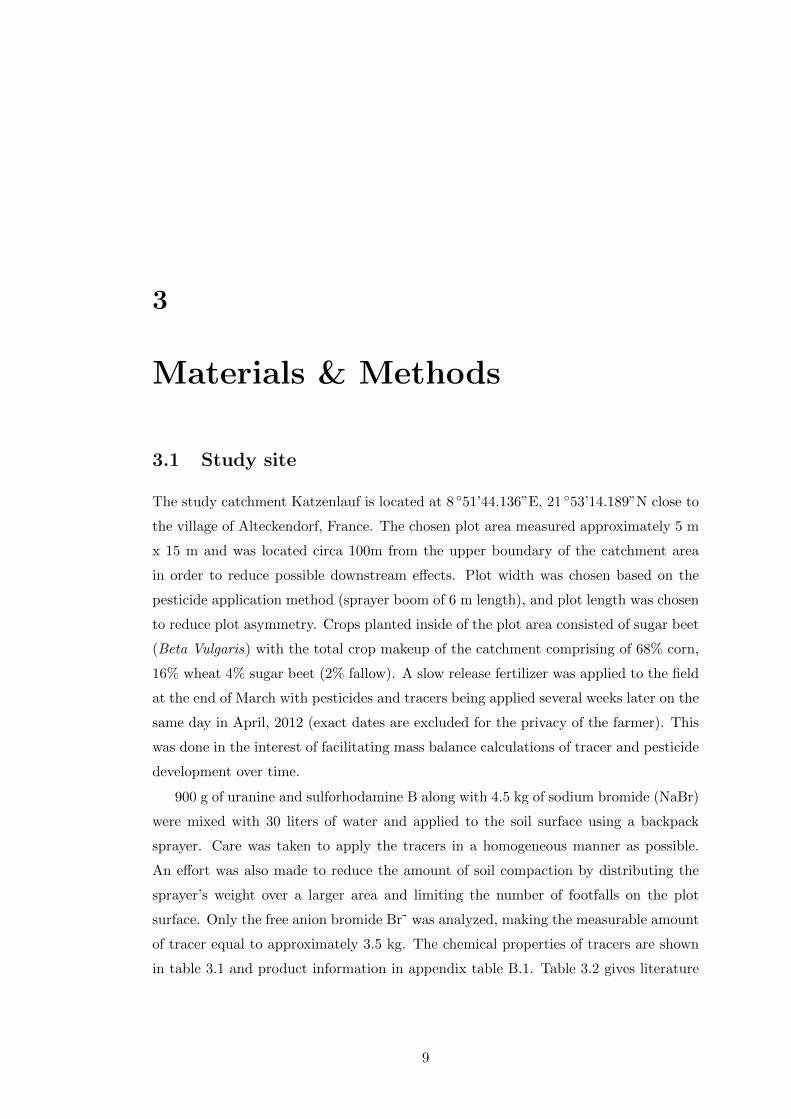
The site is characterized by circa 80% cambisols of slightly different types found in

higher catchment elevations, with the remaining 20% comprising of colluvial deposists

of the same cambisol soil at lower elevations. Cambisols are characterized by slight

or moderate weathering of parent material and by absence of appreciable quantities of

illuviated clay, organic matter, Al and/or Fe compounds. (Unesco. et al., 2006) Figure

3.1 displays the spacial distributions of the soils within the catchment.

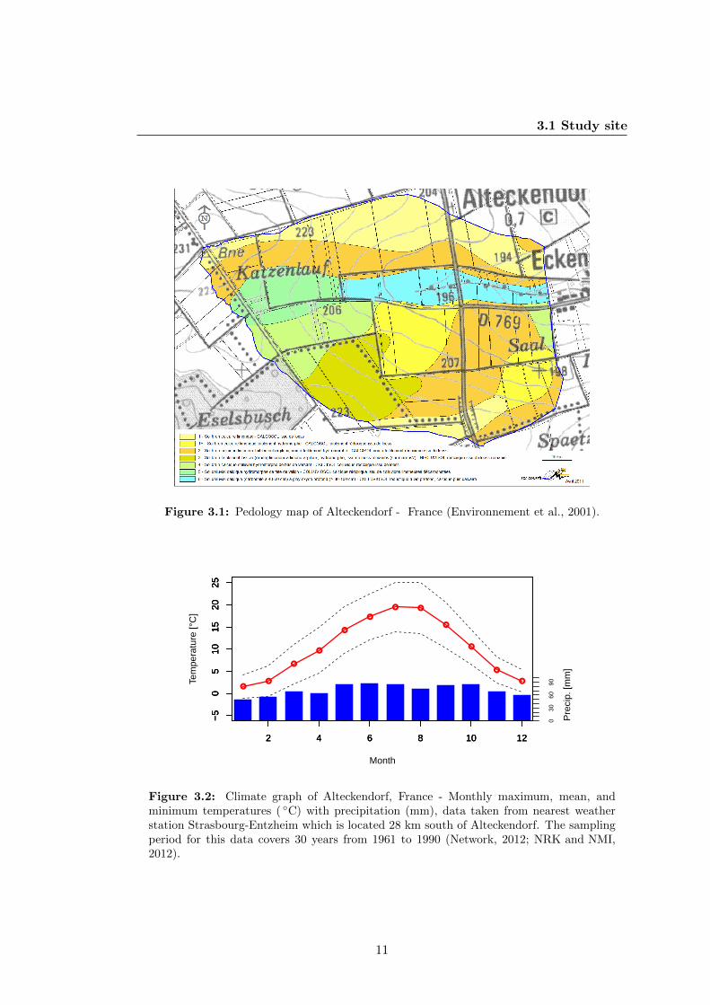
The climate of Alteckendorf, France is considered a maritime climate according to

Koppen climate classification (see Fig. 3.2). Maritime climates are defined by temper-

ate winter and summer temperatures along with evenly distributed precipitation events

10

3.1 Study site

Figure 3.1: Pedology map of Alteckendorf - France (Environnement et al., 2001).

●●

●

●

●

●

● ●

●

●

●

●

2 4 6 8 10 12

−5

05

1015

2025

Month

Tem

pera

ture

[°C

]

2 4 6 8 10 12

−5

05

1015

2025

2 4 6 8 10 12

−5

05

1015

2025

030

6090

Pre

cip.

[mm

]

Figure 3.2: Climate graph of Alteckendorf, France - Monthly maximum, mean, andminimum temperatures ( ◦C) with precipitation (mm), data taken from nearest weatherstation Strasbourg-Entzheim which is located 28 km south of Alteckendorf. The samplingperiod for this data covers 30 years from 1961 to 1990 (Network, 2012; NRK and NMI,2012).

11


throughout the year (Koppen, 1918). Alteckendorf has more precipitation events dur-

ing the months of March to July which includes most major events ie. over 20 mm/hour

(Fig. 3.2). This was considered when determining experimental dates, because spring

time runoff and erosion is much higher due to less or no crop cover and above stated

higher rainfall intensities. Furthermore, previous studies have shown that highest pes-

ticide losses in runoff occur during large intensity storms 1-2 weeks after application

(Wauchope, 1978).

3.1.2 Plot measurement devices

A list of plot measurement devices can be found in table 3.3. Figure 3.3 displays their

placement inside of the site. Values were logged at 5 min intervals for the tensiometers

and soil moisture probes, with the automatic water sampler engaging on a flow depen-

dent basis. Composite samples were produced for every 7 liters of discharge, which was

measured with an Ultrasound flowmeter at an interval of 1 min in the occurrence of

runoff.

Table 3.3: Equipment installed during the plot experiment Alteckendorf, France.

Equipment Model Evaluated parameter Mode of measurement

Ultrasound Flowmeter LOGISMA Height of water level Continuous

RefrigeratedAutomatic Sampler

Avalanche IscoMulti-Flasks NeoTek

PonselWater sampling Continuous

TensiometersT8 Long-term Monitoring

Tensiometer UMSSoil tension Continuous

Water content probesProfile Probe Type PR2

Delta-T Devices LtdVolumetric water content

of the soilContinuous

3.1.3 Catchment measurement devices

The catchment is essentially split into an upper and lower area by the department

highway 25 (D25) embankment (see fig. 3.1). Continuous discharge and hydrochemistry

data was collected at the upper catchment outlet, located at the culvert under D25,

for the duration of both experiments. No measurements or samples were taken in the

lower catchment area. Table 3.4 gives the measurement devices and their evaluated

parameters installed at the catchment and drain outlets. Composite samples for every

30 L of discharge were collected by the refrigerated automatic sampler and were kept at

12

3.1 Study site

!

!

#*

#0

""""

""

""""

""

!>

^^

Plot BoundaryDevice Hut

#0 Tipping Bucket#* Weekly Pluviometer" Tensiometer/WC probe! Porous Ceramic Cup!> Venturi¹0 6 123 Meters

^ Plot location

^ Catchment outletCatchment Boundary

Figure 3.3: Map of measurement devices at the experimental plot - Alteckendorf, France.

4 ◦C until collection to reduce degradation (biologic and photolytic) of pesticides and

dye tracers. Upon collection, samples were placed in an ice box for transport to the

laboratory where samples were filtered and either refrigerated or frozen depending on

the elapsed time before possible analysis.

Table 3.4: Equipment found at the catchment and drain outlets, evaluated parameterand type of measurement performed.

Equipment Model Evaluated parameter Mode of measurement

Limnimetric scale1 ELPOS & ELNEGStream stage and

sedimentPunctual

Ultrasound1 PCM3 NIVUS Stream stage Continuous

Hydrochemical Probe1AQUA Probe Acteon 3000

NeoTek PonselpH, Temperature, DO,

EC, RedoxContinuous

Doppler Flowmeter12150 Area Velocity Flow

Module ISCOFlow Continuous

Refrigerated

Automatic Sampler1

Avalanche IscoMulti-Flasks NeoTek

PonselWater sampling Continuous

CTD Diver2Van Essen Instruments

CTD-DiverWater Depth, EC,

TemperatureContinuous

BaroDiver2Van Essen Instruments

BaroDiverBarometric Pressure,

TemperatureContinuous

Found at 1. Catchment outlet 2. Drain outlet

13


3.1.4 Field sampling

Samples and data were collected from autonomous devices at the plot once every week

from the 17th of April until the 10th of July. Water sampling at the catchment outlet

continued from the 10th of July until the 21st of August. Punctual hydrochemistry

measurements were performed at the catchment and drain outlets as a validation mea-

sure of continuous measurements. Grab samples were taken at the plot after large

precipitation events when the automatic sampler was full. Water samples from the

plot automatic sampler were composited to determine mean concentrations for entire

runoff events. All water samples were placed on ice until arrival at the lab, where they

were refrigerated at 4 ◦C (tracers) or frozen (pesticides) until analysis to reduce bio-

and photolytic degradation.

For soil sampling the plot was divided into quadrants to provide a better areal

representation of the development of tracers and pesticides, with the NE corner being

designated as quadrant 1, then proceeding in a clockwise manner to quadrant 4 at the

NW corner (see fig. 3.4). Soil samples were taken once a week from each quadrant

of the plot from the beginning of the campaign until the 29th of May, at which point

sampling continued at an interval of every two weeks until the discontinuation of the

plot sampling campaign on the 10th of July. Each sample was comprised of a composite

of soil taken to a depth of 2 to 3 cm at several random locations within each quadrant.

Soil samples taken in the field were placed in polyethylene bags and stored in a cooler on

ice until arrival at the lab, whereupon they were frozen at −20 ◦C until analysis. This

was done to reduce degradation in samples before analysis. In addition to disturbed

surface soil samples, six 200 cm3 core samples with a depth of 5 cm, were extracted

on the 3rd of July in order to perform a site characterization of saturated hydraulic

conductivity and soil moisture retention.

Soil core samples were taken on the 12th of July before discontinuation of sampling

at the plot site using an Atlas-Copco Cobra TT percussion drill with a Van Walt soil

sampling set. A total of 12 core samples were taken to the depth of one meter with a

windowed sampler inside of the plot such that there was one sample for each tracer,

pesticide, and soil property analyses, extracted from each quadrant. Core samples

were split into sections of 0-2, 2-5, 5-10, 10-30, 30-66, and 66-99 cm. In addition

to the previous samples, 8 secondary cores were extracted for tracer analysis from

14

3.2 Tile Drain Experiment

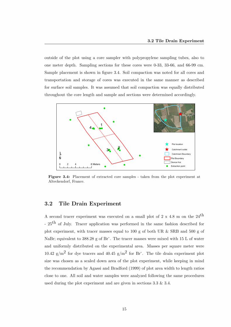
outside of the plot using a core sampler with polypropylene sampling tubes, also to

one meter depth. Sampling sections for these cores were 0-33, 33-66, and 66-99 cm.

Sample placement is shown in figure 3.4. Soil compaction was noted for all cores and

transportation and storage of cores was executed in the same manner as described

for surface soil samples. It was assumed that soil compaction was equally distributed

throughout the core length and sample and sections were determined accordingly.

!.

!.

!.

!.!.

!.

!.

!.!.!. !.!.!.

!.!.

!.!.!.!.

3 2

4 1^

^

^ Plot location


Plot BoundaryDevice Hut

!. Extraction point

¹0 4 82 Meters

Figure 3.4: Placement of extracted core samples - taken from the plot experiment atAlteckendorf, France.


A second tracer experiment was executed on a small plot of 2 x 4.8 m on the 24th

- 25th of July. Tracer application was performed in the same fashion described for

plot experiment, with tracer masses equal to 100 g of both UR & SRB and 500 g of

NaBr; equivalent to 388.28 g of Br-. The tracer masses were mixed with 15 L of water

and uniformly distributed on the experimental area. Masses per square meter were

10.42 g/m2 for dye tracers and 40.45 g/m2 for Br-. The tile drain experiment plot

size was chosen as a scaled down area of the plot experiment, while keeping in mind

the recommendation by Agassi and Bradford (1999) of plot area width to length ratios

close to one. All soil and water samples were analyzed following the same procedures

used during the plot experiment and are given in sections 3.3 & 3.4.

15


3.2.1 Site description

Figure 3.5 gives the site layout of the tile drain network and experiment performed in the

Katzenlauf catchment. Site vegetation was comprised of alfalfa (also known as lucerne;

Medicago sativa) with a mean height of approximately 20 cm. All vegetation was

removed from the experimental site before tracer application and soil was homogenized

to a depth of approximately 15-20 cm to imitate standard tilling practices employed

in the rest of the catchment. The site was located circa 35 m upslope from the drain

discharge point and directly over the tile drain network. TDR measurements were

taken at the NW corner of the experimental area and a depth of 25 cm, with water

samples and discharge measurements collected consecutively at the drain outlet.

"!;Î

"!;Î

#0

^^

^ Experimental site


Experimental siteDitchesTile drain network

#0 Tipping Bucket#* Weekly Pluviometer"!;Î Drain outlet"!;Î Catchment outlet¹0 10 205 Meters

Figure 3.5: Site of tile drain experiment - Alteckendorf, France, with description of tiledrain network found in the Katzenlauf catchment.

3.2.2 Simulated rain equipment

Simulated rain equipment was constructed and used to induce infiltration and runoff

at the experimental site. The device was similar to one fabricated by Sangesa et al.

(2010). The design consisted of 1/2 inch (1.27 cm) galvanized pipe and pipe fittings

with 4 Gardenia S-50 Pop-up Sprinkler heads (Gardena, 2012b), a manometer, and

a shut off valve. Water was supplied to the system via an electric powered pump

(Gardena, 2012a) and a generator, which was attached to a 1 m3 cistern. Figure

16


3.6 demonstrates the device set-up and its employment in the field. Water for the

experiment was supplied by the Alteckendorf community. The setup was situated at

a height of approximately 2.5 m directly above the center of the experimental plot,

running in an east-west direction.

Figure 3.6: Diagram of simulated rain device - used in the tile drain experiment atAlteckendorf, France (Sangesa et al., 2010).

A validation of the rain equipment’s homogeneity was completed before it was

employed in the field. The homogeneity of spray was evaluated by two factors, the

Christiansen’s uniformity coefficient and the distribution value, both unitless coeffi-

cients. These are both standard measures of an irrigation system’s water distribution

(Camp et al., 1997; Zoldoske and Solomon, 1988). The Christiansen’s uniformity coef-

ficient (CU) (Christiansen, 1942) is characterized by the following equation:

CU = 100 ·(

1−∑|xi − x|∑xi

)(3.1)

where CU is Christiansen’s uniformity coefficient, xi is the observed value of precipita-

tion in mm at point i of a uniformly spaced grid, and x is the mean of observed values

in mm.

17


The distribution coefficient (DU) Kruse (1978) was calculated using the equation:

DU = 100 ·( x4x

)(3.2)

where x4 is the mean of the lowest 25 percent of observations in mm of precipitation

and x is the statistical mean of observed values in mm.

3.2.3 Measurement devices and Sampling

A low tech approach was used in the measurement of runoff and discharge parameters

during the experiment. In the case of the drain discharge, flow was measured by the

use of a graduated cylinder and a stopwatch. Runoff was measured through increases

of water depth in a predefined container over a given time interval. Discharge mea-

surements were taken every 30 min and runoff measurements every 5 min on the 24th

of July during the first and second applications. The following day all measurements

were done at 5 minute intervals. Water sampling of the drain effluent was conducted

overnight and the following morning using an APEG automatic sampler at 7.5 min in-

tervals during the first hour of the tailing end of the tracer break through curves, then

at 30 min intervals in further measurements. During the campaign, water sampling was

conducted through grab sampling of drain effluent every 30 min on the 24th and every

5 min on the 25th. Soil moisture was measured at a depth of 25 cm during simulated

events at a 5 min interval, using a 6050X3K1B MiniTrase Kit (SoilMoisture Equipment

Corp. Santa Barbara, CA). Soil samples from the top 2-3 cm of soil were collected at

the end of campaign using the same randomized sampling procedure employed for the

plot experiment.

3.3 Analysis of Water Samples

Tracer analysis was performed on all samples from the plot, including samples from

the catchment after the 3rd of July. Water samples from the 3rd until the 24th of

July were taken as baseline values for calculations of tracer recovery in the tile drain

effluent. Hydrochemical testing was executed on all samples from both the plot and

the catchment. All samples were stored at 4◦C in brown glass bottles until analysis to

18

3.3 Analysis of Water Samples

reduce decay from biotic and abiotic processes. Pesticide analysis of plot and catch-

ment water samples was completed by the laboratory of hydrology and geochemistry

of Strasbourg (LHyGeS) using internal standards.

3.3.1 Bromide tracer analysis

Bromide concentrations in water samples were measured using a Dionex DX 500 Ion-

Chromatograph with the LC20 chromatography enclosure and auto-sampler (Analysis

range from 140 ppb to 100 ppm with an accuracy of 8% and an effective detection limit

of 0.018 mg/l (Dionex, 1993)). Samples were filtered with 0.7 µm glass fiber filters

and placed into 5 mL polypropylene vials for analysis. Given time restraints duplicate

measurements could not be performed and concentrations represent single measurement

values.

3.3.2 Fluorescent tracer analysis

Water samples were analyzed using a Perkin Elmer LS50B spectral fluorometer with

an extinction slit of 10 nm, an emission slit of 10 nm, a delta lambda of 22 nm, and

a scan speed of 600 nm/m. Hellma type 131-QS quartz glass Soprasil cuvettes with a

through flow pump were employed in the analysis. Samples were filtered at 0.7 µm with

glass fiber filters prior to analysis. Samples were brought to room temperature before

analyses in order to reduce temperature effects of tracer fluorescence due to different

sample and calibration temperatures (Wilson et al., 1986). pH was adjusted sample

dependent to reduce pH effects on uranine (Smith and Pretorius, 2002). Deionized

distilled water (DDW) was used in dilutions as needed. Fluorescence of DDW was was

compared with site specific blind water and showed little difference, thus no correction

was needed between diluted and non-diluted samples. Calibration curves were created

in accordance to the methodology explained in Wilson et al. (1986) (see appendix figure

A.1). Samples were analyzed in triplicates given enough solution, otherwise duplicates

were processed. Reproducibility of measurement was sample dependent and were within

the range of x ± 0.082-8.87x10-4 % for UR and x ± 0.402-6.92x10-5 % for SRB. Samples

with higher turbidity before filtering displayed higher deviations and background levels

of fluorescence than samples with lower initial turbidity. Subsequently, detection limits

were higher in such samples and sample concentrations were corrected accordingly.

19


3.3.3 Hydrochemistry testing

Hydrochemical analysis was performed on all plot and catchment water samples. Sam-

ples were analyzed for suspended solid flux (SS), organic matter in SS (OM), nitrogen

dioxide (NO2), nitrates (NO3-), ammonium (NH4

+), Phosphate (PO4-3), total inor-

ganic carbon (TIC), total organic carbon (TOC), dissolved inorganic carbon (DIC), dis-

solved organic carbon (DOC), and Phosphorous (P). Testing was completed at LHyGeS

using ISO or NF (Norme Francais) standards dependent on performed test.

3.4 Analysis of Soil Samples

All soil and core samples taken during the plot experiment were analyzed for tracer

concentrations, pH, and soil moisture content using the methods described below. The

six core samples taken on the 3rd of July were used in soil moisture retention curve

and saturated hydraulic conductivity analyses in order to characterize the physical soil

properties found at the site. Samples taken before application of pesticides and tracers

were used in the analyses of carbonaceous material and particle size. Pesticide analysis

is to be completed by LHyGeS using internal standards for all soil samples taken from

the soil surface during the tenure of the campaign and for four of the soil cores (one

for each quadrant) extracted on the 12th of July .

3.4.1 Soil pH

Soil pH testing was done in accordance with USEPA SW-846 method 9045 (USEPA,

2000) for the soil cores taken inside of the plot area on the 12th of July. Briefly, 20 g of

soil were added to an Erlenmeyer flask and mixed with 20 mL of DDW. The mixture was

then agitated by hand several times over a 30 minute period. After letting the solution

sit for an hour, allowing the majority of suspended solids to settle, the pH was measured

in the top portion of the solution with a WTW pH 597-S probe. For soil samples taken

over the course of the sampling campaign and the soil cores taken from outside of the

plot area pH testing was conducted using ISO-10390 (Carter and Gregorich, 2007; ISO,

1994) This was due to the fact that samples were frozen and had to be thawed and

dried to expedite analysis procedures. In short, 10 g. of soil was mixed with 50 mL

of DDW, agitated for 5 min and then allowed to sit for 2 hours. After the time had

elapsed the mixture was quickly agitated and the pH was measured in the liquid portion

20


of the mixture. A control of the pH probe was performed with 4.01 and 7.0 pH buffer

solutions before each use with the probe being calibrated as necessary.

3.4.2 Bulk Density and Field Moisture Content

Bulk Density and field moisture content were evaluated using the following equations

(Klute, 1986; Schack-Kirchner et al., 2009; Terzaghi et al., 1996)

Gravimetric Water Content (GWC) =(msample −mdry)

mdry∗ 100 (3.3)

V olumetric Water Content (VWC) =(msample −mdry)

Vcyl∗ 100 (3.4)

ρsoil =mdry

Vcyl(3.5)

Where GWC and VWC are in %, msample is the mass of the sample upon arrival

at the lab in g, mdry is the mass of the dried sample (105 ◦C for 48 hr) in g, Vcyl is the

volume of the sample cylinder in cm3, and ρsoil is the bulk density of the soil in g/cm3

Volumetric water content was calculated with the aid of equation 3.6 for samples taken

without defined volumes.

VWC =GWC ∗ ρsoilρwater@20 ◦C

(3.6)

with VWC and GWC given in %, ρwater in g/cm3, and ρsoil in g/cm3 being equal to

the mean bulk density of soils found at the plot.

3.4.3 Carbonaceous Material

Carbonaceous material analysis, both organic and inorganic, was calculated with a

Wosthoff-Apparatus. The apparatus introduces a previously metered sample gas into

a suitable liquid reagent of measured electrical conductivity (in this case a NaOH so-

lution). The volumetrically proportioned streams of sample gas and liquid reagent

combine, changing the conductivity of the reagent solution of which the resulting dif-

ference in conductivity of the reacted reagent solution is proportional to the concen-

tration of the sample gas being measured. Concentrations of the solution are then

21


determined by changes in the electrolytic conductivity of an absorbing solution. Con-

centrations are then converted to mg/g of substrate using mass balance considerations

(Schierjott and Eikevaag, 2012; Schlichting et al., 1995).

3.4.4 Particle size

The procedure used for the analysis of soil particle size used was the Kilmer and Alexander

(1949) pipette method which is the standard procedure of the USDA and Canadian Soil

Survey. (Carter and Gregorich, 2007; USDA, 1996) In short, samples were oven dried

at 105 ◦C for 24 hr., upon which they were passed through a 2 mm sieve separating the

fine and coarse portions of the samples. 10 g of the fine portion of the sample was then

placed in a 1 L Erlenmeyer flask and mixed with 50 mL H2O2 (30% volume fraction).

It was then capped and left overnight at room temperature. The following day the

samples were heated at 70 ◦C until all the organic material was destroyed, as needed

more H2O2 was added and the procedure repeated. After this the particles were dis-

persed using 25 mL of Na4P2O7 (C = 0.1 mol/L) and left overnight at 60 − 70 ◦C.

The following day the sample was transfered into a sedimentation cylinder (1000 mL),

shaken, and placed into a 20 ◦C water bath. A 10 mL sample was taken with a pipette

at 10 cm depth at different times according to the particle size settling rate as deter-

mined from Stoke’s law. The samples were then dried and weighed with the percentage

of each particle size calculated in relation to the sample mass.

3.4.5 Saturated hydraulic conductivity

Saturated hydraulic conductivity, or Ks value, was calculated using the falling head

method described in Head (1982). Samples cylinders were saturated through capillary

rise overnight and the following day fitted with water tight sleeves. The sleeves were

then filled with water and the time needed for the water level to move from level A to

level B was recorded. On the basis of the results the Ks value was calculated using the

following equation:

Ks =Aw

Acyl∗ lt∗ ln

(∆h0∆h1

)(3.7)

where Aw and Acyl are the area of the sleeve and sample cylinder in cm2, l is the height

of the sample cylinder in cm, t is the time in seconds, and ∆h0 and ∆h1 are the water

level at the beginning and end of the measurement in cm.

22


3.4.6 Soil Moisture Retention Curve

Analysis of six soil core samples taken on July 3rd, 2012 was done using soil wa-

ter desorption and imbibition techniques. (Carter and Gregorich, 2007; Klute, 1986;

Schack-Kirchner et al., 2009) The samples were saturated overnight in a wetting tank

using local tap water in order to bring the matric head (ψ) of samples to 0. The sample

was then weighed at saturated conditions and placed on a filter bed with a constant

head burette. A given head was then applied on the core sample and allowed time

to equilibrate, upon which it was weighed with the soil moisture content at the given

pressure head being determined by equations 3.3 and 3.4, with the mass of the sample

taken as the mass at the set pressure head. This was done for pressure head values of

0, 10, 60, 300, and 15000 hPa. A soil moisture retention curve was fit to the measured

points using the RETC program. (van Genuchten et al., 1991) All curves were fit using

the van Genuchten model with the assumption m = 1-1/n and Ks values determined

from testing. (See section 3.4.5)

3.4.7 Bromide Tracer - Desorption from soil and analysis

Bromide was extracted from the soil using a method similar to that described in

Lindau and Spalding (1984) (Herbel and Spalding, 1993; McMahon et al., 2003) In or-

der to analyze the frozen soil samples, they were allowed to thaw for one day prior to

being dried at 40 ◦C for 48 hr; then passed through a 2 mm sieve. 10 g of the < 2

mm substrate was combined with 100 mL of DDW, hand shaken for 1 minute and then

placed on a reciprocating shaking machine at 170 rpm and 26±1 ◦C for 24 hours. After-

wards, samples were transferred to glass centrifuge tubes and centrifuged at 3500g for

50 minutes. After centrifugation, an aliquot of the supernatant was taken and filtered

using 25mm syringe filters with a 0.45m cellulose acetate membrane. Finally, bromide

concentrations were measured as described in section 3.3.1. Concentrations were first

calculated as mg of bromide per L in solution and then converted to mg of Br- per g of

substrate using mass balance considerations. Sample duplicates were performed only

for core samples taken within the plot due to time constraints.

23


3.4.8 Fluorescent tracers - desorption from soil and analysis

Samples were prepared for analysis in the same manner stated in 3.4.7 for desorption of

fluorescent dyes from soil. Filtration did not affect fluorescence measurements. Super-

natant from the soil water mixture was analyzed using the procedure detailed in Section

3.3.2. Samples were brought to room temperature before analysis to reduce temper-

ature effects of tracer fluorescence. pH was adjusted dependent on initial sample pH

in order to reduce pH effects on UR. DDW was used in dilutions as needed. Calibra-

tion was executed in accordance to the methodology explained in Wilson et al. (1986)

and can be found in appendix figure A.1. Triplicate measurements of each sample

were taken and reproducibility of measurements were calculated. The reproducibility

of measurements for soil samples was within the range of x ± 0.039 - 9.5x10-4 % and

x ± 0.028 - 1.26-3 % for UR and SRB respectively.

3.5 Sorption Experiment

Batch sorption testing was performed using Alteckendorf site soil which is classified as

a hydric cambisol (see section 3.1.1) with a particle distribution of (8% sand, 64% silt,

28%clay, with 0.25 mg/g of carbon). Soil taken before the application of pesticides and

tracers was used in testing. Dyes were combined in batch testing to reflect conditions

of field application.

3.5.1 Batch sorption tests

The experimental protocol is similar to that described in German-Heins and Flury

(2000) and Mon et al. (2006). Samples were prepared by air drying them and pass-

ing them through a 2 mm sieve. Carbon was then removed using H2O2 following the

procedure described in section 3.4.4. Eight dye concentrations were used consisting

of 0.1, 1, 10, 50, 100, 200, 500, 1000 mg/l. These sample concentrations were em-

ployed since 1000 mg/l represents the applied amount of tracer on a 10 cm x 10 cm

square, which is roughly equivalent to the amount taken during each sampling ses-

sion. Two different solid to solution ratios were used for accurate measurement of

concentration changes in solution before and after shaking (Roy, 1993). The pH and

background electrolyte concentration of the batch system was adjusted with 0.1 mol/L

NaOH and CaCl2 to a pH of 9.5 and 10 mmol/L CaCl2 in order to reduce pH and ionic

24


strength effects on the analysis of samples. The samples were mixed in 100 mL brown

glass bottles, to reduce light induced decay of uranine, and placed on a reciprocating

shaking machine at 170 rpm and 26 ± 1 ◦C for 24 hours. Mikulla et al. (1997) and

German-Heins and Flury (2000) both report little difference between shaking times of

24 and 48 hr (< 1 %). Thus, 24 hr shaking times were used to expediate analysis.

Samples were then transferred to glass centrifuge tubes and centrifuged at 3500g for

50 minutes. After centrifugation, an aliquot of the supernatant was taken and filtered

using 25mm syringe filters with a 0.45m cellulose acetate membrane. A blank system

comprising of soil without dye and dye without soil were processed in the same manner

as described above. Three replicates were run of each sample including dye and soil

blanks, from which mean and standard deviations of peak values were calculated. Dye

concentrations were measured using a Perkin Elmer LS50B spectrophotometer with

the same settings used in the analyses described in section 3.3.2. Individual sorption

isotherm points were calculated from the mean concentration of triplicates according

to mass balance considerations such that:

V ∗ (C0 − C) = M ∗ (q − q0) (3.8)

where V is the volume of the sample in ml, C0 and C are the initial and equilibrium

concentrations of adsorbate in solution in mg/l, M is the mass of the substrate in g,

and q0 and q are the initial and equilibrium concentrations of adsorbate per unit mass

of absorbent in mg/g.

Distribution coefficients Kd (also known as partition coefficients) were calculated

for individual sorption points as a comparison to literature values for dyes and S-

metolachlor . Kd was calculated using the constant partition coefficient model which

is defined by the following equation:

Kd =q

C(3.9)

where Kd is the distribution coefficient in cm3/g, q is adsorbate on the solid at equilib-

rium in µg/g, and C is total dissolved adsorbate remaining in the solution at equilibrium

in µg/L (Wilhelm, 1999).

25


3.5.2 Sorption Isotherms

Two sorption isotherms, the Langmuir and Freundlich, were fit to the individual sorp-

tion isotherm points and evaluated for goodness of fit. The Langmuir isotherm is based

on a kinetic approach and assumes that adsorption takes place on a single homoge-

neous layer at a constant temperature of which each site can absorb only one atom or

molecule. It is also assumed that no phase transitions occur. (Czepirski et al., 2000;

Langmuir, 1918) The Langmuir isotherm equation is written as:

q =qm ·Ka · C1 +Ka · C

(3.10)

where q is adsorbate per unit mass of absorbent in mg/g, qm is the maximum adsorbable

value of q in mg/g, Ka is a constant (function of enthalpy of adsorption and tempera-

ture), and C is the adsorbate concentration in the solution in mg/L. Kinniburgh (1986)

states that linear transformations of the Langmuir isotherm for the derivation of equa-

tion parameters change the original error distribution; along with it the goodness of fit.

The isotherm was parameters, Ka and qm, were thus determined by fitting the data

with two different regression methods, i.e., Langmuir linearization (LL) and non-linear

least squares (NLLS) as purposed in Kinniburgh (1986) and Schulthess and Dey (1996).

The linear transformation used in calculations of Langmuir coefficients is written as:

C

q=

1

Ka · qm+

1

qm· C (3.11)

Weighted linear regression was not used to evaluate the Langmuir parameters. Kinniburgh

(1986) states that non-weighted linear regression using the Langmuir linearization re-

turns parameter estimates that lie somewhere between those obtained by assuming a

constant absolute error and a constant relative error, which often is not an unreasonable

assumption.

The Freundlich isotherm is an empirical equation, which assumes that the adsorbent

has a heterogeneous surface composed of adsorption sites with different adsorption

potentials. (Freundlich, 1909; Yetgin, 2006) The isotherm is explained by the equation:

q = Kf · C(1/n) (3.12)

where q is adsorbate per unit mass of absorbent in mg/g, Kf is a constant (function

26


of enthalpy of adsorption and temperature), C is the adsorbate concentration in the

solution in mg/L, and n is a constant. When a constant relative error is assumed the

Freundlich isotherm parameters can be estimated using the linearization:

log (q) = log (Kf ) +1

n· log (C) (3.13)

Kinniburgh (1986) states linear regression based on Eq. 3.13 gives reliable estimates

of the Freundlich isotherm parameters for the above assumptions.

27

4

Results

4.1 Plot Campaign

Several of the measurement devices at the plot malfunctioned (ie. tensiometers and soil

moisture probes) during the 3 month field campaign and no data is available for these

parameters for the tenure of the campaign. Results from the campaign include qualita-

tive water samples from runoff events and quantitative soil samples for the experiment

duration.

4.1.1 Plot Water Samples

Figure 4.1(a) depicts qualitative results of applied tracers (UR, SRB, Br-) in runoff

water samples collected during the plot experiment. The results are shown as con-

centrations per applied tracer mass (mg/L*kg). Figure 4.1(b) displays the normalized

concentrations from 0 to 1 in mg/kg*L for a representation of lower concentrations.

A table of all concentrations can be found in the appendix (Table B.2). Measured

concentrations in water samples show increases of all tracers after the rain event of

the 22nd of May. Sample sediment flux is included in both graphs, which shows a

peak value in samples taken on the 29th of May. The experimental setup for discharge

measurements was inundated during large runoff events and below the least measurable

flow during small events; thus, quantitative results could not be calculated from runoff

water samples. Pesticide data was yet to be analyzed at the time of submission of this

report. Dye tracer and pesticide data is to be compared in forthcoming reports, but is

not included in this document.

29

4. RESULTS

As a means of tracer recovery estimation for the event of the 2nd of May, measured

tracer concentrations were multiplied by the volume of standing water found in the

same hole as inundated devices. This can be found in Table 4.1. SRB demonstrates

the highest recovery rate in samples collected on the 2nd of May, with 0.032 % of

applied tracer mass and UR and Br- had values of 0.015 & 0.008 % respectively. The

same estimation was applied to the rain event of the 22nd of May. It is noted that the

volume utilized in calculations underestimates runoff from the rain event of the 22nd

given its higher intensity; its use here is only as a means of rough estimation. Tracer

recovery rates for the 22nd of May, using the above assumption are: 0.39, 0.05, and

0.11% for Br-, UR, and SRB, respectively.

A correlation matrix of water sample constituents and available physico-chemical

properties can be found in the appendix table B.5. Dye and bromide tracers show

no statistically significant correlations to physico-chemical properties, though it should

be noted that SRB displays a moderate positive correlation with rainfall. UR and

Br- demonstrate a high, statistically significant (confidence interval (CI) of 95 %),

correlation with a Pearson r-value of 0.86.

Table 4.1: Estimated tracer recovery rates for rain event of 2nd of May, 2012 at Alteck-endorf, France

Tracer Date Water Volume [m3] Conc. [mg/l] Mass [mg] % Recovered

Br 02/05/12 1.56 0.2 312.9 8.95*10-3

UR 02/05/12 1.56 8.74*10-2 136.76 0.0152SRB 02/05/12 1.56 0.1877 293.73 0.0326

Br 22/05/2012 1.56 8.75 13689.38 0.3917UR 22/05/2012 1.56 0.27 419.30 0.0466SRB 22/05/2012 1.56 0.61 961.94 0.1069

4.1.2 Soil Samples

All soil samples during the plot experiment had measurable quantities of tracers, though

fluorescence wavelength shifting occurred in both dye tracers in all samples after the

26th of June. Therefore, dye tracer quantities are only given until this date. Pesticide

analysis of soil samples was not completed before conception of this document and

comparisons will be made in forthcoming reports.

30

4.1 Plot Campaign

05

1015

Con

cent

ratio

n/S

olut

e A

pplie

d [m

g/kg

*L]

● ●

●

●

●

●

●

●

02−05 09−05 16−05 23−05 30−05 06−06 13−06 20−06 27−06 04−07 11−07

●

●

BrURSRBSS flux

2010

0P

reci

p [m

m/d

ay]

●●

●

●

● ● ● ● 02

46

8S

S fl

ux [g

/L]

(a)

0.0

0.2

0.4

0.6

0.8

Con

cent

ratio

n/S

olut

e A

pplie

d [m

g/kg

*L]

● ●

●

02−05 09−05 16−05 23−05 30−05 06−06 13−06 20−06 27−06 04−07 11−07

●

●

BrURSRBSS flux

2010

0P

reci

p [m

m/d

ay]

●

●

●

●

●

●

0.0

0.3

0.6

SS

flux

[g/L

]

(b)

Figure 4.1: Normalized tracer concentrations with suspended solid flux in water samplestaken at the plot in Alteckendorf from April to July 2012: (a) normalized concentrationsfor all events; (b) normalized concentrations from 0-1 mg/kg*L.

31

4. RESULTS

4.1.2.1 Soil Samples April - July

The development of anions at the soil surface for the duration of the experiment is

found in figures 4.3 and 4.2. Dye tracer development is witnessed in figures 4.3(c) and

4.3(d). A reduction of nearly half of all UR and SRB is seen within the first week of the

experiment reaching quantities below 0.1 mg/kg within five weeks. SRB undergoes a

less drastic reduction after the first week losing approximately 25% of its mass weekly,

whereas UR loses ∼ 50%. Calculated half-lives for UR and SRB in surface soils are

13.81 and 18.98 days, respectively. Bromide also decreases in the soil surface during the

first two weeks by more than 50%, with increases in concentrations during subsequent

dry periods. This behavior is mirrored in varying degrees by all measured anions.

After the rain event of the 22nd-23rd of May larger differences are reported in anion

and tracer concentrations between quadrants until core sampling on the 12th of July.

●

●

●

●

●

●

●

●

●

0.0

0.5

1.0

17−04 01−05 15−05 29−05 12−06 26−06 10−07

Date

Ads

orba

te/A

dsor

bant

[mg/

g]

● Zone 1Zone 2Zone 3Zone 4

2015

105

0P

reci

p [m

m/d

ay]

(a)

●

●

●● ●

●

●

●

●

0.0

0.1

0.2

0.3

0.4

17−04 01−05 15−05 29−05 12−06 26−06 10−07

Date

Ads

orba

te/A

dsor

bant

[mg/

g]


2015

105

0P

reci

p [m

m/d

ay]

(b)

Figure 4.2: Nitrate and sulfate development in the top 2 to 3 centimeters soil at Alteck-

endorf, for the period of April 17th to July 10th: (a) Nitrate (NO3-); (b) Sulfate (SO4

-2)

Uranine seems to be slightly more mobile than SRB, being transported to the

surface on the 29th of May, then decreasing in subsequent observations. SRB, on the

other hand, shows a decline in all quadrants during the complete measurement period.

Both pH and VWC exhibit decreases during dry periods and increases after rain events.

32

4.1 Plot Campaign

●

●

●

●

●

●

●

●●0

12

34

5

17−04 01−05 15−05 29−05 12−06 26−06 10−07

Date

Ads

orba

te/A

dsor

bant

[mg/

g]


2015

105

0P

reci

p [m

m/d

ay]

(a)

●

●

●

●

●

●

●

●

●

0.0

0.1

0.2

0.3

0.4

17−04 01−05 15−05 29−05 12−06 26−06 10−07

Date

Ads

orba

te/A

dsor

bant

[mg/

g]


2015

105

0P

reci

p [m

m/d

ay]

(b)

●

●

● ●●

● ● ● ●

0.0

0.5

1.0

1.5

2.0

2.5

17−04 01−05 15−05 29−05 12−06 26−06

Date

Ads

orba

te/A

dsor

bant

[mg/

g]


2015

105

0P

reci

p [m

m/d

ay]

(c)

●

●

●

●

●

● ● ● ●

0.5

1.0

1.5

2.0

17−04 01−05 15−05 29−05 12−06 26−06

Date

Ads

orba

te/A

dsor

bant

[mg/

g]


2015

105

0P

reci

p [m

m/d

ay]

(d)

Figure 4.3: Bromide, chloride, UR, and SRB in the top 2 to 3 centimeters soil for the

period of April 17th to July 10th, 2012: (a) Bromide (Br-); (b) Chloride (Cl-); (c) UR;(d) SRB.

33

4. RESULTS

●

●

●

●

●

●

●

●

●

●●

2040

6080

17−04 01−05 15−05 29−05 12−06 26−06 10−07

Date

Vol

umet

ric W

ater

Con

tent

[%]


2015

105

0P

reci

p [m

m/d

ay]

(a)

●

●

●

●

●

●

●

●

●

●

●

6.5

7.0

7.5

8.0

8.5

17−04 01−05 15−05 29−05 12−06 26−06 10−07

Date

Vol

umet

ric W

ater

Con

tent

[%]


2015

105

0P

reci

p [m

m/d

ay]

(b)

Figure 4.4: The development of volumetric water content and pH in the top 2 to 3

centimeters of soil at Alteckendorf from 17th April - 26th June: (a) VWC; (b) pH

Minimal rainfall prior to the soil sampling campaign, approximately 12 mm during a

one and a half month period, accounts for low initial VWC values.

A correlation matrix of soil constituents and physico-chemical properties can be

found in appendix table B.6. All tracers show statistically significant (CI = 95 %)

moderate negative correlations with precipitation with Pearson r-values of -0.40, -0.40,

and -0.47 for Br-, UR and SRB respectively. Further correlations of note are between

pH and soil anions besides sulfates, which display fairly strong negative correlations

of -0.59, -0.51, and -0.65 and are also statistically significant (CI = 95 %). Also, pH

and VWC have strong postive correlations (Pearson r-value = 0.75) and is statiscially

significant (CI = 95 %) All tracers show high correlations (Pearson r-values over 0.90),

with Br- and SRB the least correlative with a Pearson r-value of 0.89.

4.1.2.2 Core Samples

Due to wavelength shifting in dye tracer samples results have been excluded. Higher

concentrations of bromide in mg/g are seen to depths ranging from 5-30 cm which then

decrease with depth (see fig. 4.5(a)). The same profile is observed in chloride and

sulfate (fig. 4.5(b), 4.5(c)), with nitrate (fig. 4.5(d)) exhibiting inverse behavior in the

34

4.1 Plot Campaign

●

●

●

●

●

●


100

8060

4020

0

Dep

th [c

m]

0.00 0.05 0.10 0.15

Concentration [mg/g]

(a)

●

●

●

●

●

●


100

8060

4020

0

Dep

th [c

m]

0.010 0.012 0.014 0.016 0.018 0.020 0.022 0.024


(b)

●

●

●

●

●

●


100

8060

4020

0

Dep

th [c

m]

0.01 0.02 0.03 0.04 0.05


(c)

●

●

●

●

●

●


100

8060

4020

0

Dep

th [c

m]

1.0e−05 2.0e−05 3.0e−05 4.0e−05


(d)

Figure 4.5: Soil anions at the Alteckendorf plot to the depth of 1 meter for soil cores

extracted the 12th July, 2012:

(a) Bromide (Br-); (b) Chloride (Cl-); (c) Nitrate (NO3-); (d) Sulfate (SO4

-2).

35

4. RESULTS

first 40 centimeters of the soil column and then proceeding into an undefinable profile

between quadrants.

Cation exchange capacity (CEC) increases rapidly until a depth of 5-10 cm (fig.

4.6(a)) at which point it continues to increase more gradually with depth. pH at the

soil surface is slightly alkaline, becoming more acidic up to a depth of 5-10 cm, then

progressively becoming more alkaline with depth. Soil moisture content decreases to

an inflection point depth of 30 cm, where it begins to appreciate.

Table 4.2 gives the values of Bromide recovery from the plot soils. Bromide tracer

was not detected in any cores extracted outside of the plot area. In order to estimate

tracer masses in the soil column beneath the plot, it was assumed that all bromide

tracer infiltrated normal to the surface and no lateral flow occurred. The area assigned

to the plot was determined from GPS points of plot boundaries acquired by LHyGeS

and was split evenly into four quadrants; one for each soil core extracted. Higher tracer

masses were recovered from quadrants 3 and 4, which comprise the west side of the plot

area. Quadrants 1 and 2 exhibited much lower recovery rates than the west side, with

quadrant 2 returning only roughly 3% of the applied tracer mass. Plot slope runs in a

plane from the extreme South-west to North-east corners. In total, ∼ 87% of applied

tracer mass was recovered in the soil column.

Table 4.2: Bromide tracer recovery from the soil column for soil cores extracted on12.7.2012

Zone 1 Zone 2 Zone 3 Zone 4 Sum totalDepth Bromide St. Dev. Bromide St. Dev. Bromide St. Dev. Bromide St. Dev. Bromide St. Dev.[cm] [g] [g] [g] [g] [g] [g] [g] [g] [g] [g]

2 2.21 0.13 1.34 0.06 30.99 0.08 5.82 0.08 40.35 0.185 25.01 0.07 15.98 0.08 290.14 0.08 109.00 0.11 440.14 0.1810 410.12 0.09 78.91 0.09 491.90 0.11 344.72 0.12 1325.65 0.2030 105.58 0.07 0.00 0.00 34.03 0.06 57.88 4.02 197.50 4.0266 23.91 0.02 0.00 0.00 565.46 0.02 169.35 0.05 758.72 0.0699 0.00 0.00 0.00 0.00 24.49 0.44 244.85 0.08 269.34 0.45

Sum 566.84 0.38 96.23 0.23 1437.00 0.80 931.63 4.46 3031.70 4.55% Recovery 16.22 0.01 2.75 0.01 41.12 0.02 26.66 0.13 86.74 0.13

36

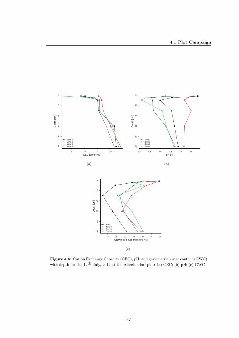
4.1 Plot Campaign

●

●

●

●

●

●


100

8060

4020

0

Dep

th [c

m]

5 10 15 20

CEC [cmol+/kg]

(a)

●

●

●

●

●

●


100

8060

4020

0

Dep

th [c

m]

6.6 6.8 7.0 7.2 7.4 7.6

pH [−]

(b)

●

●

●

●

●

●


100

8060

4020

0

Dep

th [c

m]

16 18 20 22 24 26 28

Gravimetric Soil Moisture [%]

(c)

Figure 4.6: Cation Exchange Capacity (CEC), pH, and gravimetric water content (GWC)

with depth for the 12th July, 2012 at the Alteckendorf plot: (a) CEC; (b) pH; (c) GWC

37

4. RESULTS


4.2.1 Simulated Rain Equipment

In all cases, 1 m3 of water was applied to the site area using the simulated rain de-

vice. The duration of each event was 42 ± 1 min with a mean precipitation rate of

0.74 mm/min, which is equivalent to a rain event of 31.1 ± 0.74 mm. Figure 4.7 dis-

plays rainfall event frequency for the months of March-July from a 4 year interval for

Waltenheim sur Zorn, France; which is located approximately 7 km to the South of

the Katzenlauf catchment. Most rainfall events in the area are under 5 mm for both

daily and hourly intensities. Thusly, application intensities would be similar to a two

year storm for the area, and multiple applications per day totaling 60 plus mm, would

represent an event similar to a 20 year event (see fig. 4.8). The first application was

employed as a means of wetting the area in order to reproduce conditions of a high

initial VWC (similar to several days of light rain before a large event) before a large

storm event, since this is when leaching is most likely to occur.

Precipitation [mm/day]

Fre

quen

cy

0 10 20 30 40 50

010

2030

4050

a)

Precipitation [mm/hr]

Fre

quen

cy

0 10 20 30 40

010

2030

4050

b)

Precipitation [mm/6 min]

Fre

quen

cy

0 2 4 6 8 10 12

010

2030

4050

c)

Figure 4.7: Histogram of rainfall events at Waltenheim - located 7 km to the South ofAlteckendorf, for a 4 year period, comprising of the years 2008-2011, and for the monthsof March-July a) daily b) hourly c) 6 minute intensities. Y-axis break doesn’t include alloccurrences of lower intensity events for representation of larger events.

CU and DU were evaluated using equations 3.1 and 3.2. Assuming that rainfall

for small areas is homogeneous a CU or DU value of 100 would be completely repre-

sentative of natural rainfall, with a value below 50 indicating very heterogeneous and

38


●

●

●

●2040

6080

Recurrence Interval (yr)

Max

Pre

cipi

tatio

n [m

m]

●

●

●

●

●

●

Max Daily PrecipMax Hourly Precip

1.001 1.1 1.5 5 10 20 50 100 500

Figure 4.8: Precipitation event recurrence intervals - for daily and hourly data from a 4year period (2008-2012) and the months of March-July.

unrepresentative conditions. The Center of Irrigation Technologies Fresno, California

USA rates irrigation systems with CU over 87% and DU over as 85% excellent and

those below 70% and 65% as poor. (Solomon, 1990). The mean CU and DU achieved

by the device was 82.16% & 73.65% respectively, which is fairly representative of nat-

ural precipitation conditions. Table 4.3 shows the statistics for the validation carried

out before deployment of the device in the field.

Table 4.3: Distribution statistics of simulated rain equipment calculated from an equip-ment validation performed before its use in the tile drain experiment at Alteckendorf,

France on the 24-25th of July, 2012.

Trial Mean Precipitation Christiansen’s Uniformity Distribution Uniformity[mm/min] Coefficient (DU)

(CU)

1 0.77 75.20 60.902 0.70 84.95 80.143 0.75 86.33 79.91

Mean 0.74 82.16 73.65

Figure 4.9 displays the mean rainfall distribution of the device. A fairly uniform

result is seen for a 2m x 5m area with a range of 0.7 to 0.9 mm/min. This correlates

to the area of the tile drain experiment which was 2m x 4.5m.

39

4. RESULTS

0 1 2 3 4 5 6 7

0.0

0.5

1.0

1.5

2.0

Length [m]

Wid

th [m

]

0.2

0.3

0.6

0.7

0.7

0.8

0.9

0.9

Figure 4.9: Distribution of simulated rain equipment - Contour plot of precipitation[mm/min] distribution of simulated rain equipment measured during the equipment vali-

dation on the 23rd of July, 2012.

4.2.2 Tracer Breakthrough Curves

Tracer breakthrough curves (BTC) recovery rates as witnessed in figure 4.10(a) present

tracer concentrations, normalized to the applied quantity, found in drain effluent over

the period of the experiment. Br- recoveries were approximately two times that of UR

and eight times that of SRB, during the measurement campaign. The first BTC shows

the bromide and dye tracers arriving at the same time, though dye tracer concentrations

were nominal. All tracer BTCs peak at the same time, which is slightly before the end

of irrigation inputs. It must be noted that the sampling interval at this time was 30

minutes and it is possible that the actual peak is not represented by the data. All data

was assessed with a 5 minute time step, with missing values being evaluated through

interpolation. SRB recovery during the first peak is negligent at a recovery of 0.17 %

of mass. Returns for UR and Br- during the first BTC were roughly 1.7 and 4.0 % of

mass, respectively.

Measured anion concentrations besides Br- (chloride, sulfates, and nitrates) are dis-

played in figure 4.10(b) with concentrations depicted as unitless normalized quantities

(concentration/mean concentration). An obvious peak for all anions is seen on the

24th at approximately the same time or shortly after tracer peaks. This is followed by

40


trough 2.5 to 3 hours later.

On the 25th of July, normalized UR and Br- BTCs are similar. Approximately the

same mass from the previous day was recovered in the case of Bromide and approxi-

mately 150% for UR. SRB recovery was roughly 3 times larger in comparison to the

previous day, with a nominal return of 0.61% of tracer mass. Total tracer recoveries

at the end of the measurement campaign were 7.69, 4.52, and 0.79%, for Br-, UR, and

SRB. Figure 4.11 gives a comparison of BTCs from the beginning of the rain events

until 180 minutes afterward. No tracer mass was measured within the period of 3 hours

after the first simulated rain application, though discharge and soil moisture data are

included to depict initial site conditions. Tracer BTC for the 24th of July show all

tracers arriving after the discharge peak. The BTC for the 25th gives tracer arrival

before peak discharge is measured, with the SRB peak exhibiting a lag of roughly 20

minutes compared to UR and Br-.

4.2.3 Tracer Mass Balance

Tracer recovery was calculated for the parameters measured during the tile drain exper-

iment. Table 4.4 lists the recovery rates for each of the parameters, excluding tracers

found in the soil column. Because overland flow measurements were available for only

the 3rd simulated rain application, it has been assumed that recovered values for all

events are similar. It is noted that this is an underestimation of the value, and is used

here only as a means of evaluation. Values of tracer masses found in overland flow per

single event were 0.09, 0.18, and 0.23 % for Br-, UR, and SRB, respectively. Total

tracer recoveries for measured parameters were 9.29, 5.48, and 7.79% for Br-, UR, and

SRB. No quantifiable tracer mass was measured in samples taken downstream at the

catchment outlet after the 25th of July.

Table 4.4: Mass balance calculations of tracers for measured parameters: tile drainexperiment performed, July 24-25th, 2012 Alteckendorf, France.

Tracer Applied mass [g]Recovered

mass outlet[g]

Overland flow [g] Soil Surface [g]Total Outlet +

Overland flow +Surface soil [g]

% Re-coveredTotal

Br 388.28 29.86 0.36 5.12 36.07 9.29UR 100 4.52 0.18 0.43 5.48 5.48SRB 100 0.79 0.23 6.29 7.79 7.79

41

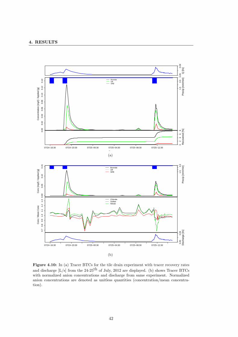
4. RESULTS

Date

0.05

0.09

Q [l

/s]

0.00

0.02

0.04

0.06

0.08

0.10

0.12

0.14

Con

cent

ratio

n [m

g/l]

/ App

lied

[g]

BromideURSRB

n

1.5

0.5

Pre

cip

[mm

/min

]

Date

02

46

8R

ecov

ered

[%]

07/24−16:30 07/24−20:30 07/25−00:30 07/25−04:30 07/25−08:30 07/25−12:30

(a)

0.00

0.05

0.10

0.15

Date

Con

c [m

g/l]

/ App

lied

[g]

BromideURSRB

Index

1.5

0.0

Pre

cip

[mm

/min

]

0.7

0.8

0.9

1.0

1.1

1.2

1.3

Con

c / M

ean

Con

c

ChlorideSulfateNitrate

0.05

0.09

Dis

char

ge [l

/s]

07/24−16:30 07/24−20:30 07/25−00:30 07/25−04:30 07/25−08:30 07/25−12:30

(b)

Figure 4.10: In (a) Tracer BTCs for the tile drain experiment with tracer recovery rates

and discharge [L/s] from the 24-25th of July, 2012 are displayed. (b) shows Tracer BTCswith normalized anion concentrations and discharge from same experiment. Normalizedanion concentrations are denoted as unitless quantities (concentration/mean concentra-tion).

42

4.3 Batch Sorption Experiment

28.3

034

.40

Soi

l Moi

stur

e [%

]

1st App 2nd App 3rd App

0.00

0.02

0.04

0.06

0.08

0.10

0.12

Time [min]

Con

cent

ratio

n [m

g/l]/

Am

ount

App

lied

[g]

BromideURSRB

50 100 150

Time [min]

0.05

0.09

Dis

char

ge [l

/s]


(a)

28.3

034

.40

Soi

l Moi

stur

e [%

]


0.00

0.02

0.04

0.06

0.08

0.10

0.12

BromideURSRB

Con

cent

ratio

n [m

g/l]/

Am

ount

App

lied

[g]

50 100 150

Time [min]

0.05

0.09

Dis

char

ge [l

/s]


(b)

Figure 4.11: Comparision of tracer BTCs seen at the drain outlet during the tile drain

experiment: (a) 1st BTC after 2 simulated rain events on the 24th (b) 2nd BTC after 1

rain event on the 25th July, 2012


Individual sorption isotherm points were evaluated using the Freundlich and Langmuir

isotherms. Best fit results were obtained from the Langmuir isotherm using NLLS re-

gression, with RMSE values of 0.00232 for UR and 0.02142 for SRB. Table 4.5 shows

the results for the other isotherms evaluated. Distribution coefficients values range

from 1.96 to 0.27 for UR and from 5.77 to 0.87 for SRB and show, in most cases, an

inverse dependency on tracer concentration (see tab. 4.6). Higher standard deviations

were calculated for lower concentrations, showing a greater imprecision in measurement,

which could account for deviations from the general pattern. Figure 4.12 reproduces

graphically the behavior of the evaluated isotherms. The inset windows show evalua-

tions at lower concentrations, which in some cases demonstrate a better fit to isotherms

other than the determined overall best fit.

43

4. RESULTS

Table 4.5: Langmuir and Freundlich isotherm coefficients and goodness of fit criteria

coefficient of determination R2 and residual root mean square error (RMSE).

DyeFreund.

Coeff. KfFreund.Coeff. n

Lang. Coeff.Ka

Max Adsorptionqm

R2 RMSE Isotherm Model

UR 0.00152 1.1862 — —0.0840

0.08554 Freundlich

— — 0.00606 0.26120.9989

0.00296 LL

— — 0.00570 0.26370.9993

0.00232 L-NLLS

SRB 0.01013 1.2410 — —0.6400

0.15572 Freundlich

— — 0.00647 0.99470.9778

0.03869 LL

— — 0.01198 0.82330.9932

0.02142 L-NLLS

Table 4.6: Distribution coefficient (Kd) [cm3/g] obtained from batch study of UR andSRB at 8 different concentrations

Batch values Kd UR [cm3/g] Kd SRB [cm3/g] Stdev. Kd UR Stdev. Kd SRB

0.1 1.377 4.902 0.044 0.1121 1.957 5.767 0.025 0.02110 1.084 4.508 0.028 0.02350 1.441 2.209 0.013 0.004100 1.246 1.984 0.011 0.002200 0.962 1.702 0.010 0.003500 0.546 1.197 0.011 0.0091000 0.272 0.867 0.016 0.006

44


●

●

●

●

●

●●

●

0 200 400 600 800 1000

0.00

0.05

0.10

0.15

0.20

C [mg/l]

q A

dsor

bate

/Ads

orba

nt [m

g/g]

Langmuir LinearizationFreundlichLangmuir NLLS

●

●

●

0 2 4 6 8 10

0.00

00.

005

0.01

00.

015

0.02

0q

Ads

orba

te/A

dsor

bant

[mg/

g]

C [mg/l]

(a)

●

●

●

●

●

●●

●

0 50 100 150 200 250 300

0.0

0.1

0.2

0.3

0.4

0.5

0.6

0.7

C [mg/l]

q A

dsor

bate

/Ads

orba

nt [m

g/g]

Langmuir LinearizationFreundlichLangmuir NLLS

●

●

●

●

●

0 2 4 6 8 10

0.00

0.02

0.04

0.06

q A

dsor

bate

/Ads

orba

nt [m

g/g]

C [mg/l]

(b)

Figure 4.12: Calculated sorption Isotherms for UR and SRB using linearized Langmuir,NLLS Langmuir and linearized Freundlich: (a) UR; (b) SRB

45

5

Discussion

Results have been presented for tracer water & soil samples from the plot along with tile

drain experiments and batch sorption tests. The aim of this study is to determine the

viability of dye tracer use as surrogates for pesticide fate and transport, in particular

uranine and sulforhodamine B for S-metolachlor. Since pesticide analysis was yet to be

completed at the time of submission of this document, comparisons are conducted with

literature values. It is noted that site specific data is needed in order to fully evaluate

tracer use. This will be addressed in continuing works related to this project.

5.1 Plot Water Samples

Tracer recovery from runoff samples using the assumptions stated in the results section

were nominal, with returns totaling 0.4, 0.06, and 0.14 % for Br-, UR and SRB. Most

Br- in runoff is collected during the event of the 22nd of May, which can be accounted

for by increases in Br- concentrations in surface soils before the event. Higher observed

tracer concentrations in water samples collected towards the end of the campaign can

explained through the deposition of tracers at the runoff catch inlet during to the rain

event of the 22nd of May. This is observed in higher concentrations of Br- found

in quadrant 4 soil core samples from the 12th of July. This behavior is seen to a

lesser degree in surface soil samples namely due to the sampling technique, in which

a composite samples for the total quadrant area were made, effectively diluting any

tracer accumulation in one area of the quadrant.

47

5. DISCUSSION

None of the tracers exhibit a high correlation with suspended solids (Pearson r-

values = -0.38, -0.25, -0.19; none statistically significant (SS) at 95 % CI), which means

tracers are more readily released to water flowing over or through the soil surface. This

is in agreement with the literature which states that runoff losses with water are the

dominate mode of transport for moderately adsorbed solutes (Baker, 1999; Gilley et al.,

1990). Br- and UR display a strong correlation (Pearson r value = 0.86; SS at 95 %

CI) in water samples, which implies similar behavior of the two tracers. In addition,

both exhibit a higher correlation (Pearson r-values = 0.64, 0.65; for Br- and UR; not

SS) to rainfall than SRB (Pearson r-value = 0.48; not SS) being attributed to their

lower Kd values. This is in accordance with the literature, which states that both Br-

and UR exhibit conservative behavior (non-adsorbing, non-retarded) in non-acidic soils

(Goldberg and Kabengi, 2010; Smith and Pretorius, 2002).

Gaynor et al. (2002) found that runoff of metolachlor accounts for a nominal portion

of total pesticide losses, comprising only 9 % of losses from measurements of leaching

and runoff. Furthermore, total pesticide losses are tied to rain events occuring within

the first 1 to 2 weeks after application irregardless of pesticide properties (Flury, 1996).

In Gaynor et al. (2002) 67 to 77 % of all metolachlor losses occurred in the first rain

event following application. Rector et al. (2003) reported S-metolachlor runoff in an

event 2 days after pesticide application that was 5.3 % of applied mass. Although there

is no large rain event during the first one to two weeks after application from which

runoff concentrations of tracers could be compared with literature values, the data does

provide insights into runoff losses even at 4-5 weeks after application. Direct comparison

with pesticide concentrations is needed to further evaluate similarities of S-metolachlor

and dye tracer similarity. Further examination of literature values provides a wide range

of photo and aerobic degradation rates for S-metoloachlor at the soil surface, 6.83 -

94.95 days for photo and 37.87 - 66 days for aerobic degradation (Costello and Hetrick,

2008). These numbers provide at least a base assumption that an increased pollution

risk exists for approximately one to two months after application; however, pollution

risk is extremely dependent on rain event size and intensity.

Potential sources of dye tracer measurement error exist for water samples collected

during low flow events before the 26th of June due to background fluorescence increases

from a high water level marking tape used prior to this date (see fig. A.2). Increases

in background fluorescence for large events was assumed to be negligible. Estimated

48

5.2 Plot Soil Samples

tracer recovery rates are more than likely overestimated due to water upslope of the plot

entering the plot area during the two major events, biasing actual measurements. This

occurred due to a failure of the boundary material. It is believed that high suspended

solid flux in samples from the 29th of May are due to counter measures taken on the

22nd of May to correct erosion problems under the runoff catch on account of the same

boundary breach. Counter measures led to there being more loose sediment directly at

the runoff catch inlet that was easily transported in subsequent runoff events.

5.2 Plot Soil Samples

All tracers show a dissipation in surface soils until the beginning of May, at which time

Br- shows an increase. Br- increases can attributed to the precipitation of salts in

surface soils. This phenomena is caused by increases in evapotranspiration resulting in

a rise of the suction force of surface soils and subsequent precipitation of salts once they

have reached the soil surface (Gran et al., 2009). This behavior is mirrored in varying

degrees by all measured soil anions. Both dye tracers followed first order kinetics with

different decay rates. Calculated half-lives for UR and SRB were 13.81 and 18.98 days,

denoting that photodegradation of UR in soils plays less of a role than one would assume

given literature values (see tab. 3.2). A possible explanation for this is migration of UR

with water away from the soil surface either through capillarity of smaller pores in the

soil matrix, or infiltration after precipitation events. Hebert and Miller (1990) found

that direct photolysis was restricted to the photic depth of soils (0.2 - 0.4 mm), while

indirect photolysis depth was slightly deeper (0.6 - 0.7 mm). In all cases photolysis was

limited to less than 1.0 mm. In a study of atrazine photodegradation in surface soils,

soil granularity, pH value, humidity, organic content, humic acid and surface-active

agents were shown to have an impact on the rate of atrazine decay (Xiaozhena et al.,

2005). These factors, in turn, likely play a role in dye tracer decay.

Negative correlations of tracer masses in surface soil and rainfall indicate that other

factors besides rainfall lead to their dissipation in surface soils. Negative correlations

of Br-, Cl, and NO3 with pH can be attributed to displacement of H and Al cations

on or near soil colloid surfaces during increases in salt concentration, which in turn,

decreases measured soil pH (Bohn et al., 2001). This is further recognized in negative

49

5. DISCUSSION

correlations of soil anions with VWC; indicating anion leaching during periods of VWC

increases and enrichment during decreases.

It is believed that decreases in measured soil anions in samples taken on the 12th

of July are due to changes in the collection procedure, in which a large quantity of soil

was taken from the soil surface in preparation for core sampling. This led to dilutions

of anion masses per soil weight and also an over representation of a single area within

the quadrant. Dilution is also believed to be a factor in the non detection of tracer

masses in soil cores taken outside of the plot, where sampling sections were larger.

Recovered bromide masses from soil cores extracted on the 12th of July indicate that

a little over one third of Br- mass was found at depths of 5-10 cm. Bromide leachate

was found to depths of one meter in two of the four cores (approximately 9 % of applied

mass), denoting a high possibility of infiltration below this depth. The majority of Br-

mass was found in quadrant four, where a large volume of water entered through a

breach in the boundary. Thus, the likelihood of macropore activation and resultant

deep percolation in this quadrant is quite high. Similar findings for S-metolachlor were

reported by Cornoi et al. (2011), in which 93 % of applied pesticide mass was recovered

in the top 15 cm of soil after 90 days.

Measured peak fluorescence of soil samples after the 26th of June were at wave-

lengths between 508-511 nm (489-491 nm are expected absorbance wavelengths for

UR) . The fluorescent peak displayed no pH dependency (ie. no change in UV ab-

sorbance); where it is assumed that increasing or decreasing pH should change the UV

absorbance of UR, with pH values below 3.5 effectively dampening all UR absorbance

(Peterson, 2010; Smith and Pretorius, 2002). Due to this SRB was effectively quenched

by peak values in the range of 508-511 nm and SRB concentrations could have been

present in samples. Wavelength shifting of UR has been recorded in other studies due

to colloids or organic content (Leibundgut et al., 2009), but there is no record of pH

independence. Samples before the 26th of June exhibited the same fluorescence in a

range of 508-511 nm, but measurable quantities of UR were found at wavelengths of

489-491 nm when solution pH was increased above 10. Also, UR fluorescence in water

samples displayed only a slight wavelength shift (measured peak at 493 nm) in sam-

ples collected on the 10th and 16th of July. This leads one to believe that erroneous

fluorescence peaks are from a soil constituent that has a low solubility, since it is not

transported by runoff events. Other possibilities could be changes in the prevalent UR

50


molecule. A study focusing on UR excitation spectra in different solutions found UR

to exhibit fluorescence at 508 nm in methanol solutions with pHs above 6.4 attributing

this behavior to a shifting of the primary UR anion from the monoanion to the dianion

(Cook and Le, 2006). This phenomena needs to be studied further if UR is to be used

in long term, surface application pesticide studies in the future.


Tracer BTC for the 24th of July show all tracers arriving after the discharge peak with

an approximate lag of 10 minutes after the second simulated rain application. Increases

in discharge can either be attributed to old water being pushed out of the soil column,

or new water arriving via macropores (Kung et al., 2000). This confirms piston flows

from the input of irrigation water, since in the case of new water tracer peaks would be

expected at the same time as the discharge peak. Furthermore, one would not expect

to see the flushing effect of soil anions exhibited by the concentration increases of Cl,

NO3, and SO4, whose peak values are at the same time as the tracers. If no flushing of

the soil matrix occurred, it would be assumed that Cl, NO3, and SO4 concentrations

would decrease with increasing discharge rates due to additions of new water. The

new water from irrigation can be seen entering the system by the observed trough in

anion concentrations approximately 6 hours after the initial simulated rain application,

evidencing the normal infiltration of water through the soil matrix.

Calculated mean Ks values from the plot characterization returned values of 552.97

± 444.25 cm/day for the plot surface. Assuming conductivity decreases with increasing

depth, it can be safely inferred that it would take longer than the observed 3 hour period

for water to reach the outlet. Thus, tracer BTC observed 3 hours after initial irrigation

application can only be attributed to preferential flows. This is affirmed by similar

tracer peak arrival times in the effluent. Under normal infiltration conditions sorptive

solutes show a retardation, with observed maximums taking place after less sorptive

solutes. Thus, if only advective transport were responsible for tracer transport, lag

times in tracer peaks should be observed, which is not the case.

SRB and UR mass recoveries from the first tracer BTC demonstrate a reduction

compared to Br-. This denotes the occurrence of adsorption during solute transport

within preferential flow pathways. If this were not the circumstance, normalized tracer

51

5. DISCUSSION

recoveries should be similar. This is most likely due to the interval between simulated

rain events, where the inactivation of macropores allowed for sorption reactions to take

place, such that in the ensuant irrigation only the unsorbed quantity of tracer was

transported in the re-activation of preferential pathways.

This finding runs counter to previous studies, which show adsorption properties

having no effect on tracer transport through preferential flow paths (Flury, 1996;

Kung et al., 2000) and is likely attributable to differences in simulated rain quantities

and durations. The assumptions made, perhaps, overestimate additions to discharge

through preferential flow; exact depths of tile drain piping and Ks values are needed to

truly substantiate claims. In addition, adsorption processes occurring in the interval

between tracer and irrigation application and between irrigation events could account

for dye tracer reductions, since in applicable studies dye and bromide tracers were

applied concurrently with irrigation water.

The BTC for the 25th shows tracer arrival before peak discharge measurement,

affirming the idea of piston flows. This is further substantiated through Cl and NO3

levels which drop almost directly after irrigation begin and display a slower return to

baseline values after the termination of irrigation, denoting inputs of irrigation water

in the effluent. SO4 levels increase for a period of approximately 30 minutes before

exhibiting the same behavior as Cl and NO3. This is explained by higher sorption of

SO4 compared to Cl in the soil matrix (Huber et al., 2012; Scanlon et al., 2009), leaving

more SO4 to be flushed out in further events. This behavior is similar to SRB, which

demonstrates a lag of roughly 20 minutes compared to UR and Br- and is common of

sorptive solutes during advective transport.

In a study comparing preferential flow under alfalfa and corn plot estimates from all

observed data suggested that 39% more bromide was leached out of the 0-30 cm zone in

the alfalfa as compared to the corn plots (Caron et al., 1996). This calls into question

the validity of the application of findings from the tile drain experiment to the entire

catchment. However, it should be noted that metolachlor can be readily transported

towards the deeper soil layer, where less degradation of the pesticide occurs, in the

presence of preferential flow (Francaviglia and Capri, 2000) and that at depths more

than 5 cm S-metolachlor was found to be more persistant than EU documented values

((Commission, 2004) EU study DT50soil = 7.6-37.6 days; (Cornoi et al., 2011) DT50soil

= 69.3 days). Thus, leaching of S-metolachlor from the soil surface via preferential flow

52


pathways or infiltration presents a high pollution risk to shallow aquifers or streams

connected to agricultural tile drain systems regardless.

Tracer recovery rates from the experiment may be underestimated due to the sam-

pling interval during the first BTC, though it is believed to have minimal effect on total

recovered tracer mass. It is also possible that BTC peaks were not accurately recre-

ated, because of the low sampling rates. Higher tracer concentrations seen at 8:30 on

the 25th were due to a leaky hose inside of the automatic sampler and values were ex-

cluded from tracer mass recoveries. Measurements of overland flow likely overestimate

discharges, because the plot area was unbound, providing a possibility for over-spray

to enter the experimental area.


A quick comparison of Kd literature to measured values of dye tracers (see tab. 3.2 and

4.6) reveals comparable sulforhodamine B values, but large differences in the sorptivity

of uranine. In both cases, sorption increases with decreasing concentration, which

mirrors S-metolachlor behavior in a study done by Cornoi et al. (2011). High organic

matter content is also a possible reason for the higher observed sorbtivity of UR. A

study by Mikulla et al. (1997) showed UR having Kd values of 10.2 in the presence

of 31.2 % organic matter. In a catchment characterization performed by LHyGeS

organic matter contents were determined to be in the range of 4.7-7.1 %. Given these

conditions it would be quite possible that higher Kd values for UR are attributed to

organic matter. In a study by Shaner et al. (2006), Kd values of S-metolachlor were

also found to be highly correlated to organic matter in the soil with Kd values ranging

from 1.58-6.93 cm3/g for organic contents 1.5-5.6 %. This suggests that S-metolachlor

would be retained in a manner closer to SRB than UR, but site specific sorption data

for S-metolachlor is needed to truly evaluate the dye tracers as surrogates, due to the

many facets of solute sorption. Failings of using Kd values to determine sorption in the

soil column are that values from batch experiments can be high relative to the extent of

sorption occurring in a real system, since water flows though the soil matrix and is not

stagnant. Kd values can also over estimate desorption, because it is normally assumed

adsorption and desorption processes are directly reversible, which normally is not the

case (Wilhelm, 1999).

53

5. DISCUSSION

Langmuir isotherms for both UR and SRB provided better estimations of sorption

than Freundlich isotherms for the given concentration range of batch studies. Compara-

ble literature values of Langmuir isotherm coefficients for S-metolachlor weren’t found,

since pesticide application concentrations were much lower than applicable dye concen-

trations, and individual isotherm points were evaluated only for Freundlich isotherms.

If further studies are to be done, an evaluation of the needed range of dye tracer concen-

tration where tracers demonstrate the same sorptivity as the chosen pesticide should

be performed. Also dye tracer application concentrations should be similar to their

pesticide counterpart. This would increase the validity of dye tracer use as surrogates

in such cases.

54

6

Conclusion

All tracers demonstrated behavior at the soil surface close to S-metolachlor values

taken from a similar study by Cornoi et al. (2011) during the first two weeks of the

plot experiment. However, degradation processes remain more or less unknown and

similar dissipation behavior could be attributed to different processes, dependent on

the constituent. Dye tracers could be used as delimiters of pesticide leaching as noted in

Sabatini and Austin (1991) and concurrently applied with pesticides if a high potential

of pesticide leaching exists. In this way secondary measures could be employed before

the arrival of pesticide peaks, and removed after them. It must be noted that tracer

masses used in this study would be cost prohibitive and further study of dye tracer use

at lower concentrations must be made, especially due to sorption behavior changes of

both dyes at low concentrations. Furthermore, photodegradation of UR could be under

level of detection when applied in small quantities reflective of pesticide concentrations

if penetration depths into the soil column are less than 0.2 mm. Bromide could also

be used to delimit pesticide transport since it arrives ahead of pesticides in almost

all cases, but increases in soil salt content could negatively impact crop production,

and needed quantities would be cost prohibitive. Further study needs to be done on

degradation and sorption processes of dye tracers if they are to be used as surrogates

in pesticide transport studies.

Given the findings of the plot experiment, dye tracers are not suited for long term

studies of pesticide losses from the soil surface. Fluorescence peak shifting and pH in-

dependence effectively masks the measurement of both dye tracers after approximately

80-90 days. It is possible that this behavior would not be seen in studies using only one

55

6. CONCLUSION

dye, but this remains unsubstantiated. Therefore, further testing comparing each dye

individually to S-metolachlor are needed in order to confirm their validity as surrogates

in surface application experiments.

The highest risk of pollution from S-metolachlor remains leaching during high in-

tensity rain storms in a period of 1 to 2 weeks following application (Flury, 1996;

Wauchope, 1978). This is further substantiated through drain experiment findings,

which show rapid transport of both dye tracers and bromide into the tile drain system

during high intensity rainfall. With effective meteorological forecasting risk of pollution

can be reduced through simple measures limiting pesticide application during periods

of potential precipitation within a week antecedent to pesticide application. It is noted

that due heterogeneity of weather patterns, risk will continue to exist and secondary

measures will be needed.

56

References

Agassi, M. and Bradford, J. (1999). Methodologies for interrill soil erosion studies. Soil and Tillage Research, 49(4):277 – 287. 6,

15

Agassi, M., Letey, J., Farmer, W. J., and Clark, P. (1995). Soil erosion contribution to pesticide transport by furrow irrigation.

J. Environ. Qual., 24(5):892–895. 2

Aley, T. (2002). Groundwater Tracing Handbook. Ozark Underground Laboratory. 10

Andreini, M. and Steenhuis, T. (1990). Preferential paths of flow under conventional and conservation tillage. Geoderma, 46:85–

102. 1, 3, 4

Baker, J. (1999). Handbook of pest management, chapter 26, pages 713–737. M. Dekker, New York. 1, 2, 3, 48

Barber, J. and Parkin, C. (2003). Fluorescent tracer technique for measuring the quantity of pesticide deposited to soil following

spray applications. Crop Protection, 22(1):15 – 21. 6

Batey, T. (2009). Soil compaction and soil management a review. Soil Use and Management, 25(4):335–345. 1

Blanquies, J., Scharff, M., and Hallock, B. (2003). The design and construction of a rainfall simulator. In International Erosion

Control Association (IECA), 34th Annual Conference and Expo. 6

Bloschl, G. and Sivapalan, M. (1995). Scale issues in hyrological modelling: a review. Hydrological Processes, 9:251–290. 3

Bohn, H., McNeal, B., and O’Connor, G. (2001). Soil Chemistry. Wiley and Sons, 3 edition. 49

Bowman, B. (1990). Mobility and persistence of alachlor, atrazine and metolachlor in plainfield sand, and atrazine and isazofos

in honeywood silt loam, using field lysimeters. Environmental Toxicology and Chemistry, 9:453–461. 5

Bowman, R. S. (1984). Evaluation of some new tracers for soil water studies. Soil Sci. Soc. Am. J., 48(5):987–993. 3

Camp, C. R., Sadler, E. J., and Busscher, W. J. (1997). A comparison of uniformity measures for drip irrigation systems.

Transactions of the ASAE, 40(4):1013–1020. 17

Caron, J., Banton, O., Angers, D., and Villeneuve, J. (1996). Preferential bromide transport through a clay loam under alfalfa

and corn. Geoderma, 69:175–191. 52

Carter, R. and Gregorich, E. (2007). Soil Sampling and Methods of Analysis, Second Edition. Canadian Society of Soil Science.

Taylor & Francis. 20, 22, 23

Cey, E., Rudolph, D., and Passmore, J. (2009). Influence of macroporosity on preferential solute and colloid transport in

unsaturated field soils. Journal of Contaminant Hydrology, 107:4557. 2

Christiansen, J. (1942). Irrigation by Sprinkling. California. Agricultural experiment station, Berkeley. University of California.

17

Cogo, N. P., Moldenhauer, W. C., and Foster, G. R. (1984). Soil loss reductions from conservation tillage practices1. Soil Sci.

Soc. Am. J., 48(2):368–373. 2

Commission, E. (2004). Review report for the active substance s-metolachlor. European Commission. 10, 52

Conservation, C. L.-R. S. W. (1993). Soil and Water Quality:An Agenda for Agriculture. The National Academies Press. 1

Cook, A. and Le, A. (2006). The effect of solvent and ph on the fluorescence excitation and emission spectra of solutions

containing fluorescein. J. Phys. Chem. Lab, 10:44–49. 51

57

REFERENCES

Cornoi, I., DeWilde, T., Cara, M., and Jitareanu, G. (2011). Sorption and leaching of s-metolachlor in surface horizons of

romania. Lucrari stiintifice, 54(2):18–22. 4, 5, 50, 52, 53, 55

Costello, K. and Hetrick, J. (2008). US EPA -Pesticides; S-Metolachlor, Pc Code 108800. USEPA. 5, 48

Czepirski, L., Balys, M. R., and Komorowska-Czepirska, E. (2000). Some generalization of langmuir adsorption isotherm. 26

Davis, S., Thompson, G., Bentley, H., and Stiles, G. (1980). Ground-water tracers - a short review. Ground Water, 1:14–23. 3

Dionex (1993). LC20 Chromatography Enclosure Operator’s Manual. Dionex Corp. 19

Dunkerley, D. (2008). Rain event properties in nature and in rainfall simulation experiments: a comparative review with

recommendations for increasingly systematic study and reporting. Hydrological Processes, 22:4415–4435. 6

Environnement, C., Lebreton-Thaler, A., and pour la relance agronomique en Alsace, A. (2001). Collines de Brumath, du

Kochersberg et de l’arriere Kochersberg: petite region naturelle n 5 : un guide pour l’identification des sols et leur valorisation

agronomique. Guide des sols d’Alsace. Region Alsace. 11

Fank, J. and Harum, T. (1994). Solute transport and water movement in the unsaturated zone of a gravel filled valley: Tracer

investigations under different cultivation types. In Publ., I., editor, Future Groundwater Resources at Ris, number 222. 3, 4

FAO (2010). Current world fertilizer trends and outlook to 2014. FAO ; UNESCO, Rome. 1

Flury, M. (1996). Experimental evidence of transport of pesticides through field soils - a review. Journal of Environmental Quality,

25:25–45. 3, 6, 48, 52, 56

Flury, M. and N.N., W. (2003). Dyes as tracers for vadose zone hydrology. Reviews of Geophysics, 41(1):2.1–2.37. 3

Francaviglia, R. and Capri, E. (2000). Lysimeter experiments with metolachlor in Tor Mancina (Italy). Agricultural Water

Management, 44:63–74. 52

Freundlich, H. (1909). Kapillarchemie. Akademische verlagsgesellschaft m.b.h. 26

Gardena (2012a). Classic garden pump 3000/4. Gardena GmbH. 16

Gardena (2012b). Pop-up sprinkler s-50 data sheet. Gardena GmbH. 16

Gaynor, J., Tan, C., Drury, C., Welacky, T., Ng, H., and Reynolds, W. (2002). Runoff and drainage losses of atrazine, metribuzin,

and metolachlor in three water management systems. Journal of Environmental Quality, 31:300308. 5, 6, 48

German-Heins, J. and Flury, M. (2000). Sorption of Brilliant Blue FCF in soils as affected by pH and ionic strength. Geoderma,

97:87–101. 24, 25

Gilley, J., Finkner, S., Doran, J., and Kottwitz, E. (1990). Adsorption of bromide tracers onto sediment. Applied Engineering in

Agriculture, 61(1):35–38. 48

Gish, T., Prueger, J., Kustas, W., Daughtry, C., McKee, L., Russ, A., and Hatfield, J. (2009). Soil moisture and metolachlor

volatilization observations over three years. Journal of Environmental Quality, 38:17851795. 5

Goldberg, S. and Kabengi, N. (2010). Bromide adsorption by reference minerals and soils. Vadose Zone Journal, 9:780–786. 48

Grace, R. and Eagleson, P. (1966). Construction and use of a physical model of the rainfall-runoff process. Technical Report 11,

Massachusetts Institute of Technology. 5

Gran, M., Carrera, J., Olivella, S., Massana, J., Saaltink, M., Ayora, C., and Lloret, A. (2009). Salinity is reduced below the

evaporation front during soil salinization. In Silva, O., editor, Estudios en la Zona no Saturada del Suelo, volume 9. 49

Grube, A., Donaldson, D., Kiely, T., and Wu, L. (2011). Pesticides Industry Sales and Usage: 2006 and 2007 Market Estimates.

USEPA. 1

Hadi, S., Leibundgut, C., Freidrich, K., and Maloszewski, P. (1997). Tracer Hydrology 97, chapter New fluorescent tracers, pages

55–62. A.A Balkema. 10

Haggerty, R., Argerich, A., and Marti, E. (2008). Development of a smart tracer for the assessment of microbiological activity

and sediment-water interaction in natural waters: The resazurin-resorufin system. Water Resources Research, 44:W00D01. 3

Head, K. (1982). Manual of Soil Laboratory Testing: Volume 2 - Permeability, Shear Strength and Compressibility Tests, volume 2.

Pentech Press Limited. 22

58

REFERENCES

Hebert, V. R. and Miller, G. C. (1990). Depth dependence of direct and indirect photolysis on soil surfaces. Journal of Agricultural

and Food Chemistry, 38(3):913–918. 49

Herbel, M. and Spalding, R. (1993). Vadose zone fertilizerderived nitrate and delta15n extracts. Ground Water, 31:376–382. 23

Hertfordshire, U. (2009). The pesticide properties database (ppdb). Agriculture and Environment Research Unit (AERU).

EU-funded FOOTPRINT project (FP6-SSP-022704). accessed 2/11/2012. 3, 5

Hrudey, S., Payment, P., Huck, P., Gillham, R., and Hrudey, E. (2003). A fatal waterborne disease epidemic in walkerton, ontario:

Comparison with other waterborne outbreaks in the developed world. Water Science and Technology, 47(3):714. 2

Huber, G., Knafla, A., Vickerman, L., and Bell, G. (2012). Summary of research on sulfate behavior in soil and groundwater:

Implications for subsoil sulfate guideline development. In PTAC Soil and Groundwater Forum, Calgary. 52

ISO (1994). ISO 10390: Soil Quality - Determination of pH. 20

Kasnavia, T., Vu, D., and Sabatini, D. (1999). Fluorescent dye and media properties affecting sorption and tracer selection.

Ground Water, 37(3):376–381. 10

Kilmer, V. and Alexander, L. (1949). Methods of making mechanical analysis of soils. Soil Science, 68:15–24. 22

Kinniburgh, D. (1986). General purpose adsorption isotherms. Environ. Sci. Technol., 20(20):895–904. 26, 27

Klute, A. (1986). Methods of soil analysis: Physical and mineralogical methods. Soil Science Society of America book series.

American Society of Agronomy. 21, 23

Knop, A. (1878). Uber die hydrographischen beziehungen zwischen der donau und der aachquelle im badischen oberlande (schluss).

Neues Jahrb. Mineral. Geol. Paleontol.,, 1878:350363. 3

Koppen, W. (1918). Klassifikation der klimate nach temperatur, niederschlag und jahresablauf. Petermanns Geogr. Mitt., 64:243–

248. 12

Kruse, E. (1978). Describing irrigation efficiency and uniformity. ASCE Journal of the Irrigation and Drainage Division, 104(1):35–

41. 18

Kung, K., Steenhuis, T., Kladivko, E., Gish, T., Bubenzer, G., and Helling, C. (2000). Impact of preferential flow on the transport

of adsorbing and non-adsorbing tracers. Soil Sci. Soc. Am. J., 64:1290–1296 1290–1296. 6, 51, 52

Lange, J., Schuetz, T., Gregoire, C., Elssser, D., Schulz, R., Passeport, E., and Tournebize, J. (2011). Multi-tracer experiments to

characterise contaminant mitigation capacities for different types of artificial wetlands. International Journal of Environmental

Analytical Chemistry, 91(7-8):768–785. 1

Langmuir, I. (1918). The adsorption of gases on plane surfaces of glass, mica and platinum. Journal of the American Chemical

Society, 40(9):1361–1403. 26

Leibundgut, C., Maloszewski, P., and Klls, C. (2009). Artificial Tracers, chapter 4, pages 57–122. John Wiley & Sons, Ltd. 50

Lindau, C. and Spalding, R. (1984). Major procedural discrepancies in soil extracted nitrate levels and nitrogen isotopic values.

Ground Water, 22:273–278. 23

McMahon, P., (U.S.), N. W.-Q. A. P., and (U.S.), G. S. (2003). Water movement through thick unsaturated zones overlying the

central High Plains aquifer, southwestern Kansas, 2000-2001. Water-resources investigations report ;03-4171. U.S. Dept. of the

Interior, U.S. Geological Survey ; Information Services. 23

Mikulla, C., Einsiedl, F., Schlumprecht, C., and Wohnlich, S. (1997). Sorption of uranine and eosine on an aquifer material

containing high organic carbon. In Kranjc, A., editor, Tracer Hydrology 97, pages 77–84. Taylor & Francis. 25, 53

Mohanty, B., Horton, R., and Ankeny, M. (1996). Infiltration and macroporosity under a row crop agricultural field in a glacial

till soil. Soil Science, 161(4):205–213. 2

Mon, J., Flury, M., and Harsh, J. (2006). Sorption of four triarylmethane dyes in a sandy soil determined by batch and column

experiments. Geoderma, 133:217224. 24

Network, T. W. (2012). Weather Statistics: Strasbourg, France. URL: http://www.theweathernetwork.com/statistics/C02102/fra0046

accessed; 7/10/2012. 11

NRK and NMI (2012). Weather statistics for Alteckendorf, Alsace France. URL:

http://www.yr.no/place/France/Alsace/Alteckendorf/statistics.html accessed; 7/10/2012. 11

59

REFERENCES

OConnell, P., Harms, C., and Allen, J. F. (1998). Metolachlor, s-metolachlor and their role within sustainable weed-management.

Crop Protection, 17(3):207–212. 5

Oliver, D. P., Kookana, R. S., Anderson, J. S., Cox, J. W., Waller, N., and Smith, L. H. (2012). Off-site transport of pesticides in

dissolved and particulate forms from two land uses in the mt. lofty ranges, south australia. Agricultural Water Management,

106(0):78 – 85. 1, 2

Olsen, L. (1995). Pesticide movement in soils: A comparison of no-tillage and conventional tillage in the beaver creek watershed

in west tennessee. Technical report, USGS. 1, 3

Peterson, C. (2010). ph dependence and unsuitability of fluorescein dye as a tracer for pesticide mobility studies in acid soil.

Water Air Soil Pollut, 209:473481. 50

Rector, R. J., Regehr, D. L., Barnes, P. L., and Loughin, T. M. (2003). Atrazine, s-metolachlor, and isoxaflutole loss in runoff

as affected by rainfall and management. Weed Science, 51(5):pp. 810–816. 48

Roth Chemicals (2011). MSDS: Sodium Bromide No. 5086. Roth Chemicals. 10

Roy, W. R. (1993). Adsorption-desorption methodologies and selected estimation techniques for transport-modeling parameters.

NATO ASI series : Series G : Ecological sciences., 32:169–188. 24

Sabatini, D. (2000). Sorption and intraparticle diffusion of fluorescent dyes with consolidated aquifer media. Ground Water,

38(5):651–656. 10

Sabatini, D. and Austin, T. (1991). Characteristics of rhodamine wt and fluoresein as adsorbing ground-water tracers. Ground

Water, 29(3):341–349. 4, 6, 55

Sanchez-Vila, X. and Carrera, J. (2004). On the striking similarity between the moments of breakthrough curves for a heteroge-

neous medium and a homogeneous medium with a matrix diffusion term. Journal of Hydrology, 294(13):164 – 175. 4

Sangesa, C., Arum, J., Pizarro, R., and Link, O. (2010). A rainfall simulator for the in situ study of superficial runoff and soil

erosion. Chilean Journal of Agricultural Research, 70(1):178–182. 5, 16, 17

Savabi, M., Golabi, M., Abou-Arab, A., and Kladivko, E. (2008). No-till farming systems, chapter Infiltration characteristics

of no-till vs. conventional tillage in Indiana and Illinois farm fields, pages 289–299. World Association of Soil and Water

Conservation. 2

Scanlon, B., Stonestrom, D., Reedy, R., Leaney, F., Gates, J., and Cresswell, R. (2009). Inventories and mobilization of un-

saturated zone sulfate, fluoride, and chloride related to land use change in semiarid regions, southwestern united states and

australia. Water Resour. Res., 45:W00A18. 52

Schack-Kirchner, H., Gaertig, T., and Petschke, C. (2009). Kurzanleitungen bodenphysikkurs. Institut fur Bodenkunde, Freiburg.

21, 23

Schierjott, P. and Eikevaag, J. (2012). Wosthoff messtechnik gmbh. URL: http://www.xn–wsthoff-90a.com/ accessed; 15/10/2012.

22

Schlichting, E., Blume, H., and Stahr, K. (1995). Bodenkundliches Praktikum: Eine Einfuhrung in pedologisches Arbeiten fur

Okologen, insbesondere Land- und Forstwirte, und fur Geowissenschaftler. Pareys Studientexte. Blackwell Wissenschafts. 22

Schulthess, C. P. and Dey, D. K. (1996). Estimation of langmuir constants using linear and nonlinear. Soil Sci. Soc. Am. J.,

60(2):433–442. 26

Shaner, D., Brunk, G., Belles, D., Westra, P., and Nissen, S. (2006). Soil dissipation and biological activity of metolachlor and

s-metolachlor in five soils. Pest Management Science, 62:617–623. 53

Sinclair, R., Rose, J., Hashsham, S., Gerba, C., and Haase, C. (2012). Criteria for selection of surrogates used to study the fate

and control of pathogens in the environment. Appl Environ Microbiol., 78(6):19691977. 4

Sinreich, M., Cornaton, F., and Zwahlen, F. (2007). Groundwater Vulnerability Assessment and Mapping: IAH-Selected Papers,

chapter Evaluation of reactive transport parameters to assess specific vulnerability in karst systems, pages 21–32. Selected

Papers on Hydrogeology Series. Taylor & Francis. 4

Smart, P. L. and Laidlaw, I. M. S. (1977). An evaluation of some fluorescent dyes for water tracing. Water Resour. Res.,

13(1):15–33. 3

Smets, T., Poesen, J., and Knapen, A. (2008). Spatial scale effects on the effectiveness of organic mulches in reducing soil erosion

by water. Earth-Science Reviews, 89(12):1 – 12. 2, 3

60

REFERENCES

Smith, S. and Pretorius, W. (2002). The conservative behaviour of fluorescein. Water SA, 28(4):403–406. 10, 19, 48, 50

Soane, B. and van Ouwerkerk, C. (1995). Implications of soil compaction in crop production for the quality of the environment.

Soil and Tillage Research, 35(12):5 – 22. 1

Solomon, K. (1990). Sprinkler irrigation uniformity. Center for Irrigation Technology. California State University, Fresno, CA.

39

Terzaghi, K., Peck, R., and Mesri, G. (1996). Soil Mechanics in Engineering Practice. A Wiley Interscience Publication. John

Wiley & Sons. 21

Tindall, J., Kunkel, J., and Anderson, D. (1999). Unsaturated zone hydrology for scientists and engineers. Prentice Hall. 3

Touma, J. and Alberge1, J. (1992). Determining soil hydrologic properties from rain simulator or double ring infiltrometer

experiments: a comparison. Journal of Hydrology, 135:73–86. 5

Unesco., Food, of the United Nations., A. O., and Office., W. S. R. (2006). World soil resources reports. 10

University, C. (1993). Extoxnet: Metolachlor. http://pmep.cce.cornell.edu/profiles/extoxnet/metiram-propoxur/metolachlor-

ext.html accessed; 1/11/2012. 5

USDA (1996). Soil survey laboratory methods manual. Number 42 in Soil Survey Investigations Report. United States Department

of Agriculture, Natural Resources Conservation Service, National Soil Survey Center, 3 edition. 22

USDA (2000). Conservation Buffers to Reduce Pesticide Losses. USDA. 1

USDA (2001). Conservation practice standard contour farming (acre) code 330. USDA-NRCS. 1

USEPA (2000). pH in Liquid and Soil SW-846 Method 9045 (Soil). USEPA. 20

van Genuchten, M., Leij, F. J., and Yates, S. R. (1991). The RETC Code for Quantifying the Hydraulic Functions of Unsaturated

Soils, Version 1.0. EPA Report 600/2-91/065. 23, 64

Vanderborght, J., Gahwiller, P., and Flahler, H. (2002). Identification of transport processes in soil cores using fluorescent tracers.

Soil Sci. Soc. Am. J., 66(3):774–787. 3, 4

Wainwright, J. (1996). Infiltration, runoff and erosion characteristics of agricultural land in extreme storm events, se france.

CATENA, 26(12):27 – 47. 2, 5

Watanabe, H., Watermeier, N., Steichen, J., Barnes, P., and Phong, T. (2007). Impacts of tillage and application methods on

atrazine and alachlor losses from upland fields. Weed Biology and Management, 7:44–54. 1, 2, 3

Wauchope, R. D. (1978). The pesticide content of surface water draining from agricultural FieldsA review1. J. Environ. Qual.,

7(4):459–472. 12, 56

Wilhelm, R. (1999). The Kd Model, Methods of Measurement, and Application of Chemical Reaction Codes. USEPA. 25, 53

Wilson, J., Cobb, E., and Kilpatrick, F. (1986). Fluorometric Procedures for Dye Tracing, chapter A12, pages 1–34. Number 3 in

Techniques of Water-Resources Investigations. USGS. 19, 24

Winchester, P. D., Huskins, J., and Ying, J. (2009). Agrichemicals in surface water and birth defects in the united states. Acta

Pdiatrica, 98(4):664–669. ii, iii

Xiaozhena, F., Boa, L., and Aijunb, G. (2005). Dynamics of solar light photodegradation behavior of atrazine on soil surface.

Journal of Hazardous Materials, B117:75–79. 49

Yetgin, S. (2006). Investigation of fuel oxygenate adsorption on clinoptilolite rich natural zeolite. Master’s thesis, Izmir Institute

of Technology. 26

Zoldoske, D. and Solomon, K. (1988). Coefficient of uniformity - what it tells us. Center for Irrigation Technology. California

State University, Fresno, CA. 17

61

Appendix A

Supplementary Figures

●●●●

●

●

●

●

●

●

●

●

0 200 400 600

020

4060

8010

0

Intensity Units [−]

Con

cent

ratio

n [µ

g/l]

R2 = 0.9963y = 0.06962 x −1.372

(a)

●●●●

●

●

●

●

●

●

●

●

●

0 100 200 300 400

020

4060

8010

0

Intensity Units [−]

Con

cent

ratio

n [µ

g/l]

R2 = 1y = 0.2293 x −1.009

(b)

Figure A.1: Fluorescence spectroscopy calibration curves with coefficient of determina-tion for (a) UR; and (b) SRB

63

A. SUPPLEMENTARY FIGURES

●●

●

●

●●

●

●

●

0 10 20 30 40 50

05

1015

2025

cm of tape/L

Trac

er C

once

ntra

tion

µg/l

●

●●

●

●●

●

●

●

05

1015

2025

UranineSRB

R2 SRB = 0.9875R2 UR = 0.9327

Figure A.2: Background fluorescence increases from high water tape - used prior to the

26th of June for the determination of runoff in the Venturi.

●

●

●

●

●

●

●

●

●

●

●

●

●

●

●

●

●

●

●

●

●

●

●

●

0 1 2 3 4 5 6 7

010

2030

4050

60

− Log Pressure Head [hPa]

Vol

umet

ric S

oil M

oist

ure

[%]

Mean pF curve

Figure A.3: Soil moisture curves - estimated using the Van Genuchen equation(van Genuchten et al., 1991) and the RETC program

64

●●

●

●

●

●

●

●

0 200 400 600 800

500

1500

2500

3500

Uranine

C [mg/l]

C/q

[g/l]

R2 langmuir = 0.9887

●

●●

●

●

●●

●

0 50 150 250

100

200

300

400

Sulforhodamine B

C [mg/l]

C/q

[g/l]

R2 langmuir = 0.9569

●

●

●

●●

●

●

●

−1 0 1 2 3

−4.

0−

3.0

−2.

0−

1.0

log C [mg/l]

log

q A

mou

nt A

dsor

bed

[mg/

g]

R2 freundlich = 0.976

●

●

●

●

●

●

●

●

−1 0 1 2

−3.

5−

2.5

−1.

5−

0.5

log C [mg/l]

log

q A

mou

nt A

dsor

bed

[mg/

g]

R2 freundlich = 0.983

Figure A.4: Langmuir and Freundlich linearizations - Langmuir and Freundlich lineariza-

tions used to obtain equation variables for UR and SRB with R2

65

Appendix B

Supplementary Tables

Table B.1: Product article numbers, CAS numbers, and producers for tracers used atAlteckendorf, France

Tracing Chemical Producer Article number CAS-No.

Uranine Simon & Werner GmbH 100982-00025 518-47-8Sulforhodamine B Waldeck GmbH 1A-006 3520-42-1Sodium Bromide Carl Roth Chemicals GmbH 5086 7647-15-6

Table B.2: Plot water sample sediment flux and tracer concentrations; suspended solids(SS), organic matter (OM), bromide (Br), uranine (UR), and sulforhodamine B (SRB)

Sample date SS flux OM %OM Conc. Br Stdev. BR Conc. UR Conc. SRB Stdev. UR Stdev. SRB[g/L] [g/L] [%] [mg/L] [mg/L] [µg/L] [µg/L] [µg/L] [µg/L]

02/05/2012 1.12 0.14 12.47 0.2 0.018 87.42 187.75 0.70 0.7115/05/2012 0.59 0.07 11.90 0.205 0.018 15.89 12.42 0.26 0.0522/05/2012 2.92 0.40 13.70 8.75 0.018 268.01 614.86 5.93 0.8929/05/2012 7.66 0.84 11.04 0.68 0.018 102.35 89.18 0.80 1.1312/06/2012 0.73 0.09 12.16 4.28 0.018 273.68 310.59 2.01 0.3219/06/2012 0.38 0.09 23.54 19.54 0.018 432.57 378.45 1.74 3.1610/07/2012 0.18 0.08 46.32 49.9 0.018 686.97 306.21 13.64 3.2916/07/2012 0.05 0.00 0.00 14.4 0.018 20.39 310.27 0.40 3.59

Table B.3: Mass balance calculations of tracers in soil surface samples: tile drain experi-ment performed, July 24-25th, Alteckendorf, France.

TracerConc.

Sampleweight

Tracer VolumeBulk

densitySoilmass

Tracermass

[mg/l] [g] [mg/kg] [m3] [kg/m3] soil mass [kg] [g]

Br 7.56 10.00 7.56 0.45 1505.12 677.30 5.12UR 0.64 10.00 0.64 0.45 1505.12 677.30 0.43SRB 9.29 10.00 9.29 0.45 1505.12 677.30 6.29

67

B. SUPPLEMENTARY TABLES

Table B.4: Saturated hydraulic conductivity (Ks) test results from plot experiment soilsurface site characterization core samples

Probe Time h0 h1 ks cm/s ks m/s Ks m/d Ks cm/d

3181 115.4 10 5 0.0300 3.00E-004 25.9480 2594.79713202 2327.2 10 5 0.0015 1.49E-005 1.2867 128.66953039 80.6 9 7 0.0156 1.56E-004 13.4700 1346.99543039 274.40 10 5 0.0126 1.26E-004 10.9125 1091.25213198 968.6 10 5 0.0036 3.58E-005 3.0915 309.14683109 541.6 10 5 0.0064 6.40E-005 5.5288 552.87963178 1214 10 5 0.0029 2.85E-005 2.4666 246.65533178 1534 10 5 0.0023 2.26E-005 1.9520 195.2018Mean 0.0064 6.40E-005 5.5297 552.9715Stdev. 0.0051 5.14E-005 4.4425 444.2540

Mean and stdev. exclude values from probe 3181;it is assumed that contact with cylinder wall was broken

Table B.5: Correlation matrices (Pearson and Spearman) of water sample constituentsand physico-chemical properties from samples taken during the tenure of the Alteckendorfcampaign

Pearson correlation coefficientsSS.flux OM Bromide UR SRB Precip.

SS.flux 1.00 0.99 -0.38 -0.25 -0.19 -0.27OM 0.99 1.00 -0.32 -0.17 -0.11 -0.20Bromide -0.38 -0.32 1.00 0.86 0.32 0.64UR -0.25 -0.17 0.86 1.00 0.45 0.65SRB -0.19 -0.11 0.32 0.45 1.00 0.48Precip. -0.27 -0.20 0.64 0.65 0.48 1.00

Pearson test significance levelsSS.flux OM Bromide UR SRB Precip.

SS.flux NA 0.00 0.35 0.55 0.66 0.52OM 0.00 NA 0.44 0.69 0.80 0.64Bromide 0.35 0.44 NA 0.01 0.45 0.09UR 0.55 0.69 0.01 NA 0.27 0.08SRB 0.66 0.80 0.45 0.27 NA 0.22Precip. 0.52 0.64 0.09 0.08 0.22 NA

Spearman correlation coefficientsSS.flux OM Bromide UR SRB Precip.

SS.flux 1.00 0.88 -0.62 -0.10 -0.10 -0.14OM 0.88 1.00 -0.29 0.24 0.14 -0.29Bromide -0.62 -0.29 1.00 0.69 0.57 0.26UR -0.10 0.24 0.69 1.00 0.55 0.24SRB -0.10 0.14 0.57 0.55 1.00 0.17Precip. -0.14 -0.29 0.26 0.24 0.17 1.00

Spearman test significance levelsSS.flux OM Bromide UR SRB Precip.

SS.flux NA 0.00 0.10 0.82 0.82 0.74OM 0.00 NA 0.49 0.57 0.74 0.49Bromide 0.10 0.49 NA 0.06 0.14 0.53UR 0.82 0.57 0.06 NA 0.16 0.57SRB 0.82 0.74 0.14 0.16 NA 0.69Precip. 0.74 0.49 0.53 0.57 0.69 NA

68

Table B.6: Correlation matrices (Pearson and Spearman) for soil constituents andphysico-chemical properties from samples taken the soil surface during the tenure of theAlteckendorf campaign.

Pearson correlation coefficientsChloride Bromide Nitrate Sulfate UR SRB GWC VWC pH Precip.

Chloride 1.00 0.49 0.49 0.68 0.38 0.35 -0.38 -0.38 -0.59 0.14Bromide 0.49 1.00 0.19 0.33 0.91 0.82 -0.64 -0.64 -0.51 -0.40Nitrate 0.49 0.19 1.00 0.08 -0.19 -0.21 -0.56 -0.56 -0.65 -0.40Sulfate 0.68 0.33 0.08 1.00 0.59 0.56 -0.27 -0.27 -0.27 0.46UR 0.38 0.91 -0.19 0.59 1.00 0.95 -0.38 -0.38 -0.20 -0.46SRB 0.35 0.82 -0.21 0.56 0.95 1.00 -0.27 -0.27 -0.08 -0.47GWC -0.38 -0.64 -0.56 -0.27 -0.38 -0.27 1.00 1.00 0.75 0.61VWC -0.38 -0.64 -0.56 -0.27 -0.38 -0.27 1.00 1.00 0.75 0.61pH -0.59 -0.51 -0.65 -0.27 -0.20 -0.08 0.75 0.75 1.00 0.35Precip. 0.14 -0.40 -0.40 0.46 -0.46 -0.47 0.61 0.61 0.35 1.00

Pearson significance levelsChloride Bromide Nitrate Sulfate UR SRB GWC VWC pH Precip.

Chloride NA 0.00 0.00 0.00 0.04 0.07 0.02 0.02 0.00 0.40Bromide 0.00 NA 0.26 0.05 0.00 0.00 0.00 0.00 0.00 0.01Nitrate 0.00 0.26 NA 0.66 0.33 0.28 0.00 0.00 0.00 0.01Sulfate 0.00 0.05 0.66 NA 0.00 0.00 0.11 0.11 0.11 0.01UR 0.04 0.00 0.33 0.00 NA 0.00 0.02 0.02 0.23 0.00SRB 0.07 0.00 0.28 0.00 0.00 NA 0.11 0.11 0.65 0.00GWC 0.02 0.00 0.00 0.11 0.02 0.11 NA 0.00 0.00 0.00VWC 0.02 0.00 0.00 0.11 0.02 0.11 0.00 NA 0.00 0.00pH 0.00 0.00 0.00 0.11 0.23 0.65 0.00 0.00 NA 0.02Precip. 0.40 0.01 0.01 0.01 0.00 0.00 0.00 0.00 0.02 NA

Spearman correlation coefficientsChloride Bromide Nitrate Sulfate UR SRB GWC VWC pH Precip.

Chloride 1.00 0.85 0.57 0.84 0.43 0.34 -0.66 -0.66 -0.72 -0.13Bromide 0.85 1.00 0.50 0.74 0.71 0.60 -0.67 -0.67 -0.66 -0.30Nitrate 0.57 0.50 1.00 0.33 -0.04 -0.17 -0.52 -0.52 -0.65 -0.31Sulfate 0.84 0.74 0.33 1.00 0.59 0.50 -0.61 -0.61 -0.51 0.07UR 0.43 0.71 -0.04 0.59 1.00 0.96 -0.20 -0.20 -0.10 -0.50SRB 0.34 0.60 -0.17 0.50 0.96 1.00 -0.10 -0.10 0.00 -0.44GWC -0.66 -0.67 -0.52 -0.61 -0.20 -0.10 1.00 1.00 0.74 0.61VWC -0.66 -0.67 -0.52 -0.61 -0.20 -0.10 1.00 1.00 0.74 0.61pH -0.72 -0.66 -0.65 -0.51 -0.10 0.00 0.74 0.74 1.00 0.48Precip. -0.13 -0.30 -0.31 0.07 -0.50 -0.44 0.61 0.61 0.48 1.00

Spearman significance levelsChloride Bromide Nitrate Sulfate UR SRB GWC VWC pH Precip.

Chloride NA 0.00 0.00 0.00 0.02 0.07 0.00 0.00 0.00 0.44Bromide 0.00 NA 0.00 0.00 0.00 0.00 0.00 0.00 0.00 0.08Nitrate 0.00 0.00 NA 0.05 0.83 0.39 0.00 0.00 0.00 0.07Sulfate 0.00 0.00 0.05 NA 0.00 0.01 0.00 0.00 0.00 0.70UR 0.02 0.00 0.83 0.00 NA 0.00 0.25 0.25 0.58 0.00SRB 0.07 0.00 0.39 0.01 0.00 NA 0.57 0.57 0.99 0.01GWC 0.00 0.00 0.00 0.00 0.25 0.57 NA 0.00 0.00 0.00VWC 0.00 0.00 0.00 0.00 0.25 0.57 0.00 NA 0.00 0.00pH 0.00 0.00 0.00 0.00 0.58 0.99 0.00 0.00 NA 0.00Precip. 0.44 0.08 0.07 0.70 0.00 0.01 0.00 0.00 0.00 NA

69

Declaration

I herewith declare that I have produced this paper without the prohibited

assistance of third parties and without making use of aids other than those

specified; notions taken over directly or indirectly from other sources have

been identified as such. This paper has not previously been presented in

identical or similar form to any other German or foreign examination board.

The thesis work was conducted from May 10th, 2012 to November 12th,

2012 under the supervision of Prof. Dr. Jens Lange at the Institut fur

Hydrologie; Albert-Ludwigs Universitat Freiburg.

Freiburg im Breisgau, 12th November, 2012

Brian J. Sweeney

using hydrological tracers to study pesticide fate and ... · using hydrological tracers to study...

Documents