using helium as hydrogen surrogate for … · list of tables ... space with one vent ... table 4-1...
TRANSCRIPT

USING HELIUM AS HYDROGEN SURROGATE FOR SAFETY ANALYSIS
RELATED TO HYDROGEN LEAKS FROM RESIDENTIAL FUEL CELL SYSTEMS
Erdem Kokgil
A Thesis
in
The Department
of
Building, Civil and Environmental Engineering
Presented in Partial Fulfillment of the Requirements
For the Degree of Master of Applied Science (Building Engineering) at
Concordia University
Montréal, Québec, Canada
September 2015
© Erdem Kokgil, 2015

CONCORDIA UNIVERSITY
School of Graduate Studies
This is to certify that this thesis is prepared
By: Erdem Kokgil
Entitled: Using Helium as Hydrogen Surrogate for Safety Analysis Related to Hydrogen
Leaks from Residential Fuel Cell
and submitted in partial fulfillment of the requirements for the degree of
Master of Applied Science (Building Engineering)
complies with the regulations of the University and meets the accepted standards with respect to
originality and quality.
Signed by the final examining committee:
Dr. Theodore Stathopoulos Chair
Dr. Hua Ge Examiner
Dr. Hoi Dick Ng Examiner
Dr. Liangzhu Wang Supervisor
Dr. Lyes Kadem Supervisor
Approved by
Chair of Department or Graduate Program Director
2015
Dean of Faculty

iii
ABSTRACT
Using Helium as Hydrogen Surrogate for Safety Analysis Related to Hydrogen Leaks from
Residential Fuel Cell Systems
Erdem Kokgil
One of the most critical barrier against residential hydrogen fuel cell systems is the unintended
release of hydrogen in an enclosure that causes fires and explosions, especially when the gas
concentration level exceeds certain amount in the ambient air. Scientists are using helium as a
surrogate to investigate and observe the dispersion behaviour of hydrogen in case of a leak.
However, it has been found that there are differences between hydrogen and helium
concentrations before the plumes become stable, during the initial stages of the gas release. At
present, the similarity of the hydrogen and helium plumes depend only on experimental results
and observations. This thesis proposes a theoretical model of a point source light gas plume and
developed a new theoretical model for the similarity of hydrogen and helium plumes.
In order to better understand the dispersion behavior of the hydrogen gas in an enclosure,
experiments were conducted in a 1/4 sub-scale residential garage model. Helium gas was
released inside the model with various experimental configurations. Helium concentrations were
measured by thermal conductivity sensors to observe the effects of natural and mechanical
ventilation. For natural ventilation cases, it is found that volumetric flow rate, injector height,
release direction and release times had significant effects on helium concentration levels inside
the enclosure. For the mechanical ventilation case, high fluctuations of concentration levels
were observed at the sensors inside the plume and the maximum concentration level did not have
a significant difference inside the plume compared to the same case with natural ventilation. On
the other hand, the maximum concentration level outside the plume had vital differences, forced
ventilation caused maximum concentration level to stay below the lower hydrogen explosion
limit.

iv
ACKNOWLEDGEMENT
I would like to thank to my supervisor Dr. Liangzhu Wang for his encouragement, support and
guidance during my studies. I would also like to thank Dr. Lyes Kadem for his co-supervision and
valuable guidance.
Additionally, I would like to thank Dr. Wael Salah and Dr. Hoi Dick Ng for their valuable
contribution and support in my study. I would also like to thank Mr. Joseph Hrib and Mr. Luc
Demers for their service during the experiments.
I offer my regards and respect to my colleague Jiaqing He for his contribution to my study. I
would like to thank my other colleagues Guanchao Zhao and Sherif Goubran for their assistance
and support. Most importantly, I would also thank to my family for their support during my
studies.

v
Table of Contents
LIST OF FIGURES ..................................................................................................................... viii
LIST OF TABLES .......................................................................................................................... x
NOMENCLATURE ...................................................................................................................... xi
1. INTRODUCTION ...................................................................................................................... 1
1.1. Background .......................................................................................................................... 1
1.2. Overview of Hydrogen Fuel Cells ....................................................................................... 1
1.3. Types of Hydrogen Fuel Cells ............................................................................................. 4
1.3.1. Molten Carbonate Fuel Cells ......................................................................................... 4
1.3.2. Phosphoric Acid Fuel Cells ........................................................................................... 5
1.3.3. Proton Exchange Membrane Fuel Cells ........................................................................ 6
1.3.4. Solid Oxide Fuel Cells ................................................................................................... 7
1.4. Hydrogen Fuel Cell Residential Applications around the World ........................................ 9
1.5. Safety Issues of Hydrogen Leakages ................................................................................. 12
1.6. Research Objectives ....................................................................................................... 14
1.7. Thesis Outline ................................................................................................................. 15
2. LITERATURE REVIEW ......................................................................................................... 16
2.1. Release and Dispersion of a Buoyant Gas in Partially Confined Spaces ........................... 16
2.2. Experimental Study of the Concentration Build-Up Regimes in an Enclosure without
Ventilation ................................................................................................................................. 20
2.3. Helium Dispersion Following Release in a 1/4-Scale Two-Car Residential Garage ......... 24
2.4. Hydrogen Leakage into Simple Geometric Enclosures ..................................................... 27
2.5. CFD Benchmark on Hydrogen release and Dispersion in Confined, Naturally Ventilated
Space with One Vent ................................................................................................................. 31
2.6. Summary ............................................................................................................................ 36
3. THEORY .................................................................................................................................. 38
3.1. Similarity of Hydrogen and Helium Plumes ...................................................................... 38
3.2. Assumptions ....................................................................................................................... 40
3.3. Analytical Expressions ....................................................................................................... 41
3.3.1. Equations of Mass and Momentum ............................................................................. 42
3.3.1.1. Conservation of Mass .......................................................................................... 42
3.3.1.2. Conservation of Momentum ................................................................................ 43
3.3.2. Solution of the Two Differential Equations ................................................................ 44
3.4. Hydrogen and Helium Plume Similarity Equation ............................................................ 46

vi
4. METHODOLOGY ................................................................................................................... 48
4.1. Sub-Scale Residential Garage Experiment Methodology .................................................. 48
4.1.1. Sub-scale Model .......................................................................................................... 48
4.1.1.1. Geometry.............................................................................................................. 48
4.1.1.2. Helium Supply ..................................................................................................... 50
4.1.1.3. Gas Sampling System .......................................................................................... 51
4.1.1.3.1. Calibration of Sensors ................................................................................... 51
4.1.1.4. Mechanical Ventilation ........................................................................................ 53
4.1.2. Experimental Method .................................................................................................. 55
4.1.2.1. Series of Tests ...................................................................................................... 55
4.1.2.2. Experimental Procedure ....................................................................................... 57
5. RESULTS AND DISCUSSION ............................................................................................... 58
5.1. Sub-Scale Residential Garage Tests ................................................................................... 58
5.1.1. Natural Ventilation Cases ............................................................................................ 58
5.1.1.1. Volumetric Flow Rate .......................................................................................... 58
5.1.1.2. Release Location .................................................................................................. 61
5.1.1.3. Injector Height ..................................................................................................... 63
5.1.1.4. Release Direction ................................................................................................. 67
5.1.1.5. Gas Release Time ................................................................................................ 68
5.1.2. Mechanical Ventilation Case ....................................................................................... 69
5.1.2.1. ASHRAE Standard 62.1 Exhaust Rate for Residential Garages ......................... 69
5.2. CFD Comparison of Hydrogen and Helium Plume Similarity .......................................... 72
5.2.1. CFD Model .................................................................................................................. 72
5.2.1.1. Geometry.............................................................................................................. 72
5.2.1.2. Parameters of the Simulation ............................................................................... 73
5.2.2. Comparison of CFD Predictions to Experimental Data .............................................. 76
5.2.2.1. Helium Concentrations ........................................................................................ 76
5.2.3. Comparison for Hydrogen and Helium Plume Similarity Using the CFD Model ...... 77
5.2.3.1. Same Volumetric Flow for Hydrogen and Helium .............................................. 77
5.2.3.2. Volumetric Flow Rates Based on Equation 3.15 ................................................. 78
5.3. Summary ............................................................................................................................ 79
6. CONCLUSION AND FUTURE WORK ................................................................................. 81
6.1. Conclusion .......................................................................................................................... 81
6.2. Future Work ....................................................................................................................... 82

vii
REFERENCES ............................................................................................................................. 84
APPENDIX A – SENSOR MEASUREMENT GRAPHS ........................................................... 87
APPENDIX B – HELIUM CONCENTRATIONS FOR 20 CASES ........................................... 89
APPENDIX C – FAN CALIBRATION MEASURMENTS ...................................................... 100

viii
LIST OF FIGURES
Figure 1-1 Schematics of a hydrogen fuel cell [Source: www.fuelcells.org]. ................................ 2
Figure 1-2 Schematics of MCFC [Source: http://mypages.iit.edu/~smart/garrear/fuelcells.htm]. . 5
Figure 1-3 Schematics of PAFC [Source: http://mypages.iit.edu/~smart/garrear/fuelcells.htm]. .. 6
Figure 1-4 Schematics of PEMFC .................................................................................................. 7
Figure 1-5 Schematics of SOFC [Source: http://mypages.iit.edu/~smart/garrear/fuelcells.htm]. .. 9
Figure 1-6 RHEIN system for 8 homes, configuration of a fuel cell system [15]. ....................... 10
Figure 1-7 Full-scale test of 18.6% hydrogen/air mixture ignited with a car inside the garage
[41]. ............................................................................................................................................... 13
Figure 2-1 Experiment setup [22]. ................................................................................................ 17
Figure 2-2 Schematic representation of the flow in an enclosure with a point source plume [23].
....................................................................................................................................................... 21
Figure 2-3 Experimental set-up, top view (left) and side view (right) [23]. ................................. 22
Figure 2-4 Experimental setup of 1/4-scaled a two car residential garage [24]. .......................... 24
Figure 2-5 Data from the 20 enclosures modeled, the ratio between helium and hydrogen
concentration near the ceiling [33]. .............................................................................................. 30
Figure 2-6 Leakage in 1/2 scale garage. Double vent garage door, gas supply opposite side of
garage door, supply rate: 2700lt/h. [33]. ....................................................................................... 31
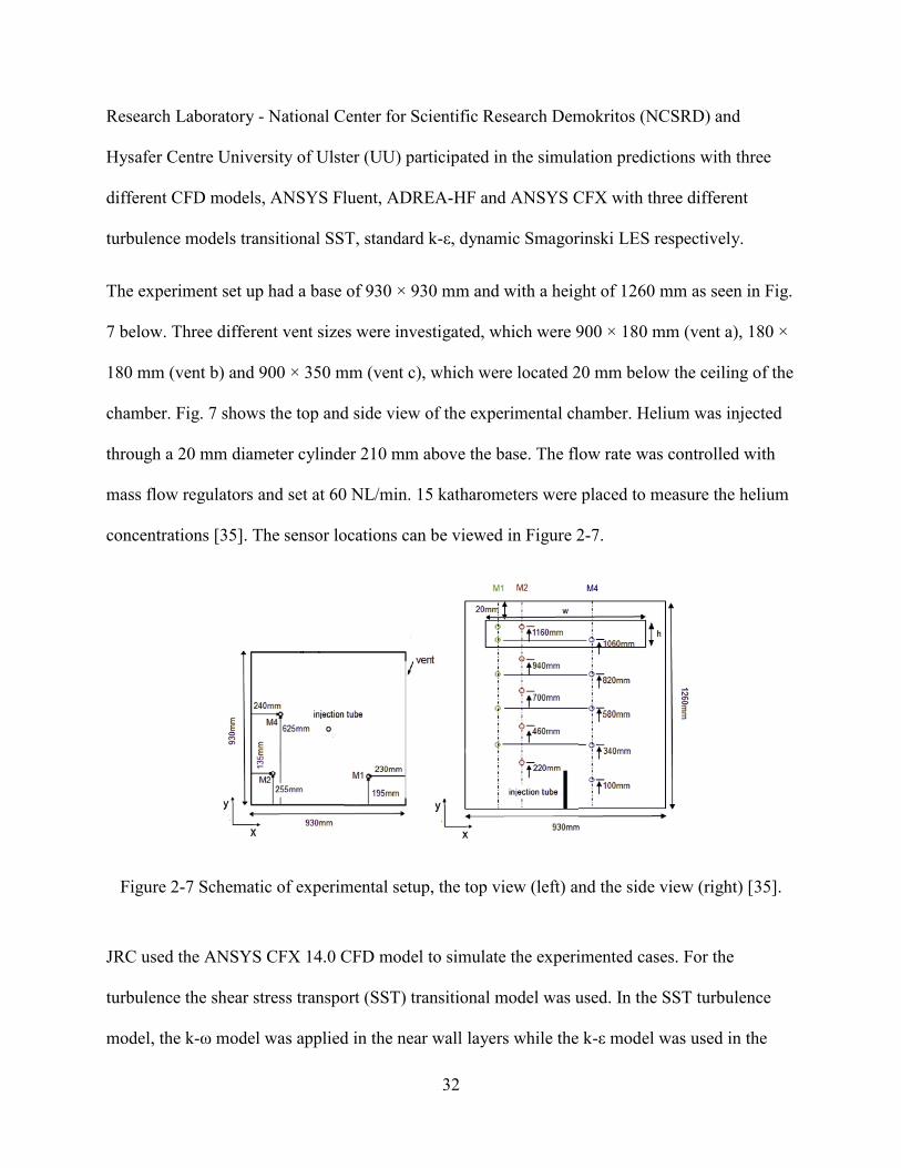
Figure 2-7 Schematic of experimental setup, the top view (left) and the side view (right) [35]. . 32
Figure 2-8 Vent a: comparison of the predicted helium concentration vs. experimental for sensor
M4 [35]. ........................................................................................................................................ 34
Figure 2-9 Vent b: comparison of the predicted helium concentration vs. experimental for sensor
M4 [35]. ........................................................................................................................................ 35
Figure 2-10 Vent c: comparison of the predicted helium concentration vs. experimental for
sensor M4 [35]. ............................................................................................................................. 35
Figure 3-1 Schematics of Hydrogen and Helium Plumes. ............................................................ 39
Figure 3-2 Schematic of light gas plume from a point source [36]. ............................................. 41
Figure 4-1 Sub-scale 1/4 residential garage model at Concordia University. .............................. 49
Figure 4-2 Helium mass flow controller. ...................................................................................... 50
Figure 4-3 XEN-5310 Helium Sensor (left) XEN-85000 USB Readout (right). ......................... 51
Figure 4-4 Calibration Setup for 8 sensors and 2 USB outputs. ................................................... 52

ix
Figure 4-5 Location of the sensors inside the model. ................................................................... 52
Figure 4-6 Fan speed calibration. .................................................................................................. 54
Figure 5-1 Comparison for different volume flow rates (a) 5L/min (b) 10L/min and (c) 15L/min
....................................................................................................................................................... 60
Figure 5-2 Location of the helium sensors and injector for Case 2. ............................................. 61
Figure 5-3 Comparison for different release locations (a) Corner release (b) Center release. ..... 62
Figure 5-4 Sensor and helium injector locations for Case 13. ...................................................... 63
Figure 5-5 Comparison for different release heights (a) 0.55m (b) 0.123m. ................................ 64
Figure 5-6 Comparison for different release directions (a) Upwards (b) Downwards. ................ 66
Figure 5-7 Comparison for different release times (a) 300 sec (b) 900 sec (c) 1800 sec. ............ 69
Figure 5-8 Comparison of mechanical ventilation to natural ventilation (a) Mechanical ............ 71
Figure 5-9 Numerical model of sub-scale enclosure. ................................................................... 73
Figure 5-10 Volumetric helium concentration at the end of 2700 seconds. ................................. 75
Figure 5-11 Comparison of predicted helium concentrations to measured data for Case 15. ...... 76
Figure 5-12 Hydrogen simulation vs helium simulation - Same Volumetric Flow. ..................... 78
Figure 5-13 Hydrogen simulation vs helium simulation – Equation 3.15. ................................... 79

x
LIST OF TABLES
Table 1-1 Summary of current hydrogen fuel cell types [2]. .......................................................... 4
Table 1-2 Fuel Flammability Comparisons [20]. .......................................................................... 13
Table 4-1 ASHRAE 62.1 Minimum Exhaust Rates [38]. ............................................................. 53
Table 4-2 Experimental cases. ...................................................................................................... 56
Table 5-1 Simulation parameters. ................................................................................................. 74
Table 5-2 Hydrogen and helium volumetric flow rates for simulations. ...................................... 77
Table 5-3 Percentage accuracy for Case 15. ................................................................................. 79

xi
NOMENCLATURE
ACH Air changes per hour
QH2 Hydrogen volumetric flow rate, m3/s
QHe Helium volumetric flow rate, m3/s
Qair, H2 Air entrainment rate to hydrogen plume, m3/s
Qair, He Air entrainment rate to helium plume, m3/s
Qexhaust rate Exhaust fan volumetric flow rate, m3/s
Bgas Buoyancy flux of gas, m4/s3
g Acceleration due to gravity, m/s2
ṁplume Mass flow rate of the plume, kg/s
u Upwards velocity of the plume, m/s
C Volumetric concentration of the gas
b Radius of the plume, m
α Ambient air entrainment coefficient
ρHe Helium density, kg/m3
ρH2 Hydrogen density, kg/m3
Acronyms
MCFC Molten Carbonate Fuel Cell

xii
PAFC Phosphoric Acid Fuel Cell
PEMFC Proton Exchange Membrane Fuel Cell
SOFC Solid Oxide Fuel Cell
CFD Computational Fluid Dynamics
LES Large Eddy Simulation

1
1. INTRODUCTION
1.1. Background
Demand for energy is increasing due to the rapidly growing world population. In order to supply
energy for this dramatic increase, new environmentally friendly and sustainable technologies
need to be developed. Fossil fuel based energy causes environmental problems that have
motivated researchers on more environmentally conscious alternative fuels. Among the many
possibilities of renewable energy solutions such as wind and solar; hydrogen is a promising
energy carrier, which can be used for fueling vehicles and powering residential homes without
producing greenhouse gas emissions.
William Grove developed the fuel cell first more than 150 years ago. He had the idea to
investigate the reverse version of the electrolysis. Around the 1840’s the popularity of fuel cells
increased by the investigations of Ludwig Mond and Charles Langer. The first successful
implementation was by Francis Bacon in 1932. The major application of the fuel cell was
developed by NASA in 1950’s to use as electric generators for space crafts. Today, there are a
number of large companies who play a key role in for the fuel cell technology via making large
investments, in order to supply energy for residential homes and transportation [1].
1.2. Overview of Hydrogen Fuel Cells
This section briefly explains the components of the hydrogen fuel cell. Figure 1-1 below is a
representation of a fuel cell. It is an electrochemical device that combines hydrogen and oxygen
to produce electricity and the byproducts are heat and water. The hydrogen can be obtained from
any hydrocarbon fuel such as natural gas, gasoline, diesel, or methanol. The oxygen is acquired

2
from air around the fuel cell. Since fuel cells are electrochemical devices operating without
combustion, they do not generate combustion emissions [2].
Figure 1-1 Schematics of a hydrogen fuel cell [Source: www.fuelcells.org].
A hydrogen fuel cell can provide heat as a byproduct that is released from the process, which is
called cogeneration. The fuel cell does not contain any moving parts, making it a quiet and
reliable source of power, electricity, heat, and water. [3]
Each fuel cell system consist of individual fuel cells that are stacked and located at the center of
the fuel cell equipment or power plant. Moreover, according to the type of fuel cell, there may be
a fuel processing section of the equipment, which is separate form or integral to the cell stack.
This system produces power in the direct current (DC) form, therefore a converter is needed to
change the current form DC to alternating current (AC). Regardless, all fuel cell power plants
contain these components and thus, the assembly of them into the system is crucial [4].

3
The fuel processor is the section where relatively pure hydrogen is provided to the fuel cell. The
hydrogen can be obtained from fuels such as steam reforming natural gas, coal gasification,
biogass and liquefied petroleum gas and diesel [5, 6 and 7]. Additionally, electrolysis of water
can be another source for hydrogen, combining the system with solar photovoltaic panels can
produce enough energy for the electrolysis [8, 9 and 10].
Hydrogen gas is constantly supplied to the electrodes where an electrochemical reaction occurs
to produce an electric current. The battery consists of two electrodes, namely anode and cathode,
which produce electricity. The anode, which is the negative portion of the fuel cell, conducts the
electrons released from the hydrogen molecules so that they can be used in an external circuit.
The anode has channels that diffuse the hydrogen gas equally to the surface of the catalyst,
splitting the hydrogen molecules into positively charged ions, releasing an electron. The
positively charged ions transfer to the electrolyte and the negatively charged electrons
transported through the external circuit to produce electric energy. On the other hand, the
cathode, which is the positive portion of the fuel cell, also has channels that distribute the oxygen
supply from air to the surface of the catalyst. It conducts the electrons back from the external
circuit, where they can combine with the hydrogen ions again and produce water [2, 3].
It should be noted that, one single fuel cell can produce around 0.7 volts. In order to increase the
voltage, many different fuel cells need to be combined to form a fuel cell stack. The fuel cell
stack is installed into a fuel cell system along with a fuel reformer, power electronics, and
controls. If there are more cells in the stack, there will be more power output. The term stack
power density determines the amount of power produced for an area of a fuel cell. [2]
4
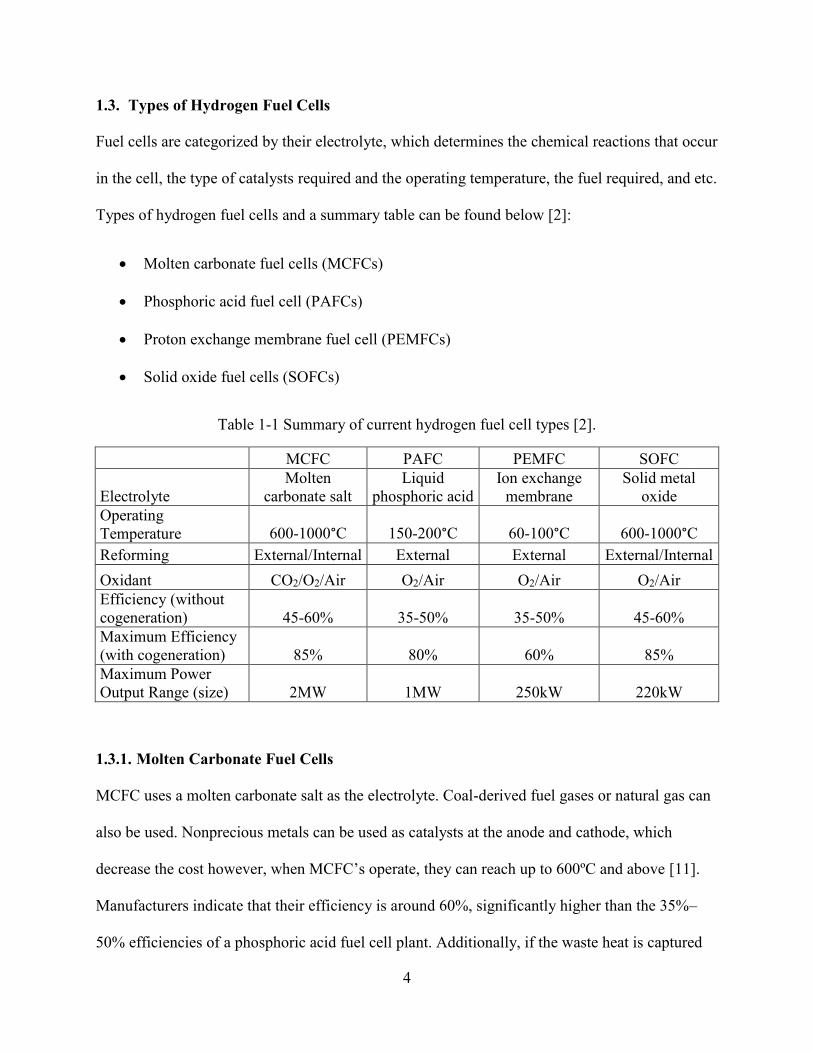
1.3. Types of Hydrogen Fuel Cells
Fuel cells are categorized by their electrolyte, which determines the chemical reactions that occur
in the cell, the type of catalysts required and the operating temperature, the fuel required, and etc.
Types of hydrogen fuel cells and a summary table can be found below [2]:
Molten carbonate fuel cells (MCFCs)
Phosphoric acid fuel cell (PAFCs)
Proton exchange membrane fuel cell (PEMFCs)
Solid oxide fuel cells (SOFCs)
Table 1-1 Summary of current hydrogen fuel cell types [2].
MCFC PAFC PEMFC SOFC
Electrolyte
Molten
carbonate salt
Liquid
phosphoric acid
Ion exchange
membrane
Solid metal
oxide
Operating
Temperature 600-1000°C 150-200°C 60-100°C 600-1000°C
Reforming External/Internal External External External/Internal
Oxidant CO2/O2/Air O2/Air O2/Air O2/Air
Efficiency (without
cogeneration) 45-60% 35-50% 35-50% 45-60%
Maximum Efficiency
(with cogeneration) 85% 80% 60% 85%
Maximum Power
Output Range (size) 2MW 1MW 250kW 220kW
1.3.1. Molten Carbonate Fuel Cells
MCFC uses a molten carbonate salt as the electrolyte. Coal-derived fuel gases or natural gas can
also be used. Nonprecious metals can be used as catalysts at the anode and cathode, which
decrease the cost however, when MCFC’s operate, they can reach up to 600ºC and above [11].
Manufacturers indicate that their efficiency is around 60%, significantly higher than the 35%–
50% efficiencies of a phosphoric acid fuel cell plant. Additionally, if the waste heat is captured

5
and used, total efficiency can go up to 85% [2]. Figure 1-2 below represents a schematic of a
MCFC.
Even though MCFC’s name might imply otherwise, carbon monoxide (CO) and carbon dioxide
(CO2) poisoning are not an issue and CO2 can be used as fuel. This property makes MCFC’s
more attractive for fueling with gases made from coal. Although they have more resistance to
impurities than other fuel cell types, scientists are searching for new ways to make MCFC’s
more resistant to impurities [2].
The main disadvantage of current MCFC technology is the strength. The high temperatures and
the corrosive electrolyte decrease cell life. Scientists are also focusing on corrosion-resistant
materials to increase cell life without decreasing the efficiency [3].
Figure 1-2 Schematics of MCFC [Source: http://mypages.iit.edu/~smart/garrear/fuelcells.htm].
1.3.2. Phosphoric Acid Fuel Cells
PAFC’s contain an anode and a cathode made from a platinum catalyst on carbon paper, and a
silicon carbide matrix that holds the phosphoric acid electrolyte. They are more durable to the
impurities than PEMFC’s. Carbon monoxide sticks to the platinum catalyst at the anode causing

6
decrease of the fuel cell's efficiency [11]. Their efficiency can go up to 85% when used with the
cogeneration of heat and electricity although without the cogeneration their efficiency is around
35% to 50% [2]. Figure 1-3 below represents a schematic of PAFC.
Today, more than 200 PAFC systems have been installed all around the world in commercial
buildings such as; hospitals, nursing homes, hotels, office buildings, schools, utility power
plants, military bases, airport terminal, landfills, and waste water treatment plants. Most of them
are 200-kW PC25 fuel cell power plant produced by the ONSI Corporation, one example is the
police station in New York City's Central Park. The PAFC system in Japan is the largest
application, which operates with 11-MW power. Most of the reference projects of PAFC’s have
operated for more than 40,000 hours without any disruption [2].
Figure 1-3 Schematics of PAFC [Source: http://mypages.iit.edu/~smart/garrear/fuelcells.htm].
1.3.3. Proton Exchange Membrane Fuel Cells
PEMFC’s operate with a fluorocarbon ion exchange with a polymeric membrane as the
electrolyte. They operate at low temperatures compared to other fuel cell types and are able to
change and control their power output to meet fluctuating power demands. Therefore, with these

7
properties, PEMFC’s offer a good solution for light-duty vehicles, buildings, and smaller
applications [3]. Figure 1-4 below shows the schematics of PEMFC’s.
PEMFCs operate at lower temperatures, around 80°C, which have a faster warm-up and allows
for a quick start. This results in less thermal stress for system components. On the other hand,
lower temperature operation requires a platinum catalyst to separate the hydrogen electrons and
protons [12]. The platinum catalyst is not durable to carbon monoxide which then requires the
need to have an additional reactor to decrease carbon monoxide in the fuel gas only if the
hydrogen is produced from a carbon based fuel. Scientists are looking for different catalyst
formations that are more resilient to carbon monoxide [2]. PEMFC manufacturers indicate that
system efficiencies vary from 35% to 50% and, with thecapture and use of byproduct heat, the
system efficiency can go up to 60%.
Figure 1-4 Schematics of PEMFC
[Source: http://www.nist.gov/mml/msed/functional_polymer/fuelcell.cfm].
1.3.4. Solid Oxide Fuel Cells
The technology is still developing for SOFC’s due to the use of thin layer of zirconium oxide as
a solid ceramic electrolyte. They reach higher temperatures around 1000ºC while operating,
which prevents using a precious-metal catalyst. Moreover, SOFC’s are able to reform fuels

8
internally, which allows them to use different type of fuels and reduce the related costs. This is
the reason why SOFCs are a good solution for applications that require high power.
SOFCs are sulfur resistant allowing them resilience to carbon monoxide, which can also be used
as fuel [13].
Additionally, SOFCs can also use gases made from coal or other gas-fired fossil fuels. However,
high-temperature operation creates disadvantages, which causes slow start-up and requires
significant thermal insulation to preserve heat and protect the people working in the vicinity.
This can be acceptable for utility applications but not for transportation and mobile applications.
The high operating temperatures also require high heat resistance on materials. The most crucial
part for SOFC’s is the development of low-cost materials with high heat resistance for high
operating temperatures [2].
The electric efficiency of unpressurized SOFC is around 45% and according to Argonne
National Laboratory, pressurized efficiency can go up to 60%. The efficiency of power
generation can go up to 85% with the use of cogenerated heat [2].

9
Figure 1-5 Schematics of SOFC [Source: http://mypages.iit.edu/~smart/garrear/fuelcells.htm].
1.4. Hydrogen Fuel Cell Residential Applications around the World
Due to its power generation with high efficiency and low environmental impact, many
researchers around the world have conducted experiments and simulations to investigate the
performance of the fuel cells for residential applications. Japan is one of the leading countries for
the application of hydrogen fuel cells in residential areas [14].
The application of fuel cells for residential houses started in the early 2000’s in Japan. General
system components are fuel cell stacks, fuel processors that generate hydrogen from natural gas,
heat recovery equipment, and a boiler. The implementation of fuel cell systems did not require
additional infrastructure which is why consumer acceptance was rapid in Japan. On the other
hand, there are limitations in terms of efficiency and flexibility. One study in Japan suggested the
implementation of a regional hydrogen energy interchange network (RHEIN), which enables
consumers for the interchange of hydrogen, electricity, heat and hot water in residential homes.
They suggested the fuel processors should be separated from the fuel cell stacks. In order to
observe and investigate, they proposed a system of eight homes, see Figure 1-6 for the detailed

10
schematics. One of the greatest advantages of this system is, it is easy to install that requires
minimum additional investment and can be combined with systems installed in other groups of
homes. Furthermore, a mathematical model was developed to investigate the effect of RHEIN on
energy cost reduction for homes and CO2 emission. [15].
Figure 1-6 RHEIN system for 8 homes, configuration of a fuel cell system [15].
11
Different cases on the number of fuel cells and fuel processors with and without energy
interchange were investigated in terms of energy cost and CO2 emission. The results showed that
the energy interchange simultaneously improved both the objectives. It had advantages both
energy cost and CO2 reduction. The operation of the fuel cells should be determined according to
the electricity and heat balance demand and different operational strategies should be applied for
different seasons. Another similar study conducted in Japan had very similar results showing the
benefit of the interchange network for hydrogen, electricity, heat and hot water in residential
homes [16].
Besides Japan, there are also other studies about fuel cell systems from other countries. A study
was performed to determine the feasibility of PEMFC for residential cooling system in Ghardaia,
located in the southern region of Algeria [17]. Residential homes in Ghardaia have a
considerable problem of cooling during hot summers for a long period of the year. In this study,
the PEMFC sub-system and the absorption sub-system were simulated by using the Unit of
Applied Research in Renewable Energies in Ghardaia’s residence data. According to the
operating data of the PEMFC, the most suitable generation temperatures of single-effect
absorption chiller system was set between 70 and 85°C. Simulation results showed that the best
achieved COP of the absorption subsystem is 0.72 with a maximum cooling capacity of 4.86kW.
When the PEMFC maximum electrical power was reached, the methane consumption was
0.0017 m3, total system efficiency was determined to be 70% and the PEMFC efficiency was
determined to be 40%. They concluded that using PEMFC sub-system and a single effect H2O-
LiBr absorption chiller sub-system, offered an efficient system to cool residences located in
Ghardaia, Algeria [17].
12
An additional feasibility study of the fuel cell system was investigated in Malaysia. A cost
comparison was conducted between cogeneration system fuel systems to the conventional grid
energy system. Two different models, grid-independent and cogeneration system are simulated
using Homer 1 software to decide if the energy demand compensates the electric and thermal
loads of the residence. Two cases, with and without battery pack were simulated to observe the
effect of power generation of fuel cell systems. Results indicated that cogeneration system can
decrease the energy usage by 30-40%, which enables that fuel cell systems can become an
alternative energy source for residential homes in the near future [18].
Likewise, another study was conducted in New Zealand to investigate requirements of fuel cells
in residential houses, where the power demand ranges from 1 to 10kW. PEM, SOFC and PAFC
technologies were investigated in terms of energy costs. Results indicated that all types of fuel
cells have cost target around 500-700 EUR/kW. The most suitable application of fuel cells in
New Zealand was suggested where grid connections are not available or very expensive. During
the time of the study, in 1999 all types of fuel cell costs were estimated to be around 1000
EUR/kW. It was estimated that the market for fuel cell generators in New Zealand is
approximately 1250 units per year [19].
1.5. Safety Issues of Hydrogen Leakages
As seen from aforementioned studies around the world, hydrogen fuel cell technology has an
untapped potential for powering residential homes in the near future. However, there are several
issues to overcome, one predominantly being the cost. Moreover, hydrogen is extremely
flammable with in the concentration limits of 4-74% by volume in air, which can create safety
challenges for public acceptance. Although, hydrogen is not more or less dangerous than other
flammable fuels such as gasoline and natural gas, it is imperative that all flammable fuels must

13
be carefully handled. Besides, hydrogen is the lightest gas and diffuses very fast, almost 3.8
times faster than natural gas and 2 times faster than helium [20]. Table 1-2 below shows the
comparison of hydrogen to other flammable fuels.
Table 1-2 Fuel Flammability Comparisons [20].
Hydrogen Gasoline Vapor Natural Gas
Flammability Limits (in air) 4-74% 1.4-7.6% 5.3-15%
Explosion Limits (in air) 18.3-59 % 1.1-3.3% 5.7-14%
Ignition Energy (mJ) 0.02 0.2 0.29
Flame Temperature in air (°C) 2045 2197 1875
Stoichiometric Mixture (most
easily ignited in air) 29% 2% 9%
These special properties of hydrogen makes safety issues the most critical barrier against the
public opinion. Therefore, the science community identifies unintended release and
concentration levels of hydrogen in an enclosure causing fires and explosions as the most crucial
problems. Scientists are investigating accident scenarios of hydrogen leakage in indoor
residential areas by studying dispersion behavior of hydrogen buoyant plume, spatial behavior of
hydrogen concentration level in an enclosure and the effects of natural and mechanical
ventilation for the mentioned behaviors (Figure 1-7).
Figure 1-7 Full-scale test of 18.6% hydrogen/air mixture ignited with a car inside the garage
[41].

14
Many researchers conduct full and sub scale experiments to understand the hydrogen dispersions
in enclosures, due to the safety and economic reasons, generally helium was chosen as a
surrogate for those experiments. Helium is the second lightest gas with non-toxic and non-
reactive properties. Swain et al. [21] showed that helium gas can be used to predict the
distribution and concentration of hydrogen gas leakage scenario. However, it has also been found
that there are differences between hydrogen and helium concentrations before the plumes
becomes stable, during the initial release of the gases. Currently, the similarity of the plumes
between two gases only rely on experimental results, without a theoretical model. Since
hydrogen safety is very crucial for fuel cell technology, a new theoretical model between
hydrogen and helium plumes urgently needs to be investigated.
In this thesis, a theoretical model was developed for a point source light gas plume in order to
find the analytical expressions to appropriately correlate hydrogen plumes to helium plumes. The
model between hydrogen and helium were compared with the results of advanced computational
fluid dynamic (CFD) software. Furthermore, in order to understand the effects of natural and
mechanical ventilation, sub-scale experiments were conducted and concentrations of helium
were measured at various points.
1.6. Research Objectives
The research objectives of this thesis are:
Determine and compare the effects of natural and mechanical ventilation for the
concentration of helium in sub-scaled model.
With various experimental cases, the effects of, volumetric flow rate, release location,
injector height, release direction, release time along with effect of forced ventilation will
be observed.

15
Develop a theoretical expressions for a point source plume and determine a new
theoretical model for the similarity of helium and hydrogen plumes.
With this new model, similarity between helium and hydrogen plumes can be identified.
This model can be used for further studies of helium experiments that will predict
hydrogen dispersion.
Compare the numerical result for several cases with experimental measurements of sub-
scaled model in order to investigate hydrogen helium plume similarity.
1.7. Thesis Outline
Chapter 2 presents a literature review of experimental and numerical studies for predicting
hydrogen dispersion using helium gas. Sub-scale experiments along with numerical studies were
found to provide assurance to use helium to simulate hydrogen leakage.
Chapter 3 presents a theoretical model to determine the properties of a point source light gas
plume. The properties are radius, upward velocity, volumetric concentration and the plume
density at any given height. Determination of the hydrogen and helium plume similarity model is
also presented.
Chapter 4 introduces a sub-scale physical model built to investigate a typical two car residential
garage at Concordia University building an envelope lab. The model geometry, helium supply,
gas sampling system and experimental method are described in details.
Chapter 5 analyzes the results of various cases of sub-scale experiment. A brief overview is
presented for the CFD Fluent model. For several cases, results are compared with the CFD
predictions.
Chapter 6 presents the conclusions and suggested future work.
16
2. LITERATURE REVIEW
In this chapter, several cases of hydrogen dispersion in an enclosure are presented along with the
comparison of experimental and CFD simulation results. In all the cases, helium was used as a
substitute of hydrogen. A summary of the effects of flow rates, vent size and location, gas supply
direction and location are investigated. The goal is produce a general consensus on the
dispersion behaviour and concentration levels of hydrogen in an enclosure while using helium.
2.1. Release and Dispersion of a Buoyant Gas in Partially Confined Spaces
Prasad et al. [22] from the Fire Research Division, National Institute of Standards and
Technology (NIST) evaluated the ability of FDS (Fire Dynamics Simulator), a CFD code to
simulate the number of experiments on predicting the dispersion and mixing behavior of
hydrogen, when accidentally released in a partly limited space. In order to conduct the
experiments safely, helium was chosen as a surrogate. In a sub-scaled residential garage
enclosure, helium gas was released from two different heights, with two different opening
locations, different flow rates and release times. Seven different sensors on the same vertical axis
with different heights above the floor measured helium gas concentrations.
In this study, based on the dimensions of two car residential garage 6.1 × 6.1 × 3.05 m, roughly
1/4 scale experimental chamber with interior dimensions of 1.5 × 1.5 × 0.745 m was constructed
from 1.25 cm thick plexiglas (Figure 2-1).

17
Figure 2-1 Experiment setup [22].
Helium supply was located at 207 mm height, above the center of the floor with a diameter of
36mm and a cross sectional area of 10.2 cm2. Helium flow was controlled by a mass flow
controller. Helium flow rates were calculated and scaled to exemplify the leakage rate of a
typical 5 kg of hydrogen from a fuel tank in 1 hour and 4 hours, which were respectively 14.95
L/min and 3.74 L/min [22].
This article describes a typical residential garage as not air-tight especially considering the
garage door and windows. Therefore, their study suggested that for a sub-scale chamber, opening
sizes were chosen to have areas that provide minimum ventilation requirements for residential

18
garages, which was 3 air changes per hour (ACH) with pressure differential of 4 Pa. An opening
with size of 2.34 × 2.32 cm (cross-sectional area of 5.43 cm2) and another opening with size of
1.56 × 2.32cm (cross-sectional area 3.62 cm2) were used to compare experimental data and
simulation predictions.
Prasad et al. [22] used NIST Fire Dynamic Simulator (FDS) to simulate the experiments
conducted in this study. FDS is a CFD code that was developed for computing fire driven flows.
Both in experiment and simulation results; as helium was released into the experimental setup,
the buoyant plume rose directly to the ceiling with a horizontal spread behavior. Air inside the
chamber was pushed outwards through the holes as helium concentration increase towards the
ceiling. Results indicate that the helium variation in helium concentration in the horizontal
direction was relatively small outside the plume. For example, when the helium supply was
located at the center, 21 cm above of the floor, with one hole on the side wall; the average
difference between the maximum concentrations of experimental data and numerical results were
less than 3.3%.
Furthermore, Prasad et al. conducted differently configured cases to understand the effect of each
configuration on the concentration of helium. Results showed that increasing the mass flux of
helium by 10%, increased the predicted concentration of helium by 7.4%, for both sensors which
are located 9.3 cm (Sensor 1) and 65 cm above the floor (Sensor 7).
One case showed that, when the cross-sectional area of the helium supply was reduced by 25%,
the predicted helium concentration increased by 2.5% for both sensors. Hence, decreasing the
helium supply in a cross sectional area caused an increase in the flow velocity to maintain a
constant mass flux but did not create a significant difference in the concentration level of helium
[22].

19
In another case, moving the helium supply 72.5 cm above floor, very close to the ceiling, had a
substantial effect on the measured concentrations because the distance to ceiling and time
available for air entrainment into the helium plume were reduced. As a result, the helium
concentration measured for sensor 1 was significantly lower and then for sensor 7 was
significantly higher [22].
In order to observe the effect of different size of openings, an opening with a size of 2.34 × 2.32
cm (cross-sectional area of 5.43 cm2) versus another opening with a size of 1.56 × 2.32 cm
(cross-sectional area 3.62 cm2) were used to compare experimental data and simulation
predictions. It was found that changing the size of the hole on the wall for predicting the helium
concentration was not very sensitive. Only slight differences were observed during the dispersion
phase, which was less than 2.5%. Even though the size of the openings do not have a large effect
on the predicted helium concentration, the location of the leaks have higher effect on mixing and
dispersion. The results show that the location of the leaks have a large effect on the gas
concentration inside the experimental chamber [22].
Increasing the mesh density inside the plume and around the openings can improve the
comparison between numerical simulations and experimental data. Although the sensors were
located outside the plume, grid size used in the simulations was suitable for predicting the helium
concentration. If the sensors were located inside the plume, smaller mesh size would be needed
for a better prediction of helium concentration. Results show that coarse mesh and fine mesh
approaches were relatively close during the release phase, whereas, the relative difference
occurred between them during the dispersion phase, which was approximately 7.5%. This shows
that the helium concentration can increase as the grid density increases and can better estimate
the experimental data [22].

20
2.2. Experimental Study of the Concentration Build-Up Regimes in an Enclosure without
Ventilation
Cariteau et al. [23] from Laboratoire d’Etude Experiméntale des Fluides, conducted experiments
of simplified cases to investigate the dispersion behavior of hydrogen in confined spaces without
ventilation. As in the previous experiment, helium was used as substitute of hydrogen due to
safety reasons. Various configurations, where the source of the helium gas was jet or plume were
studied. The aim was to quantify the effects of a leak from a fuel cell system within three
different distinct regimes; stratified, stratified with a homogeneous upper layer and homogenous.
This study cites that the magnitude of Richardson number determines whether the flow is jet or
plume. Even though in the case where the number was smaller than one, the flow at the exit was
jet like. On the other hand, if the velocity was decreased, it might allow a transition to a plume
like flow for a certain distance above the gas supply. During this type of flow, the gas dispersed
in the enclosure and led to the variation of density in the enclosure. Furthermore, it was noted
that there were two zones inside the chamber during such a gas release, which namely the forced
plume vertical upward and the rest of the volume. The density distribution inside the chamber
throughout the gas filling, was particularly reliant on supply conditions. As the effects of gravity
dominate, the distribution of density was considered by a stable vertical stratification.

21
Figure 2-2 Schematic representation of the flow in an enclosure with a point source plume [23].
As seen in Figure 2-2, the plume was developed vertically on the ceiling until after it was
deflected horizontally by the edges of the enclosure. A descending vertical flow filled the entire
horizontal section of the enclosure. A horizontal border was formed over the division between
the upper part of the enclosure where the injected gas was gathered and the lower part where the
density remains unchanged. This border was called the filling front. In the upper layer, the
mixture density was reduced from the border to the ceiling. The filling front moved down as the
gas is injected.
The enclosure used in this study has a square floor with 93 × 93 cm and 1.26 m height. Helium
was supplied through 5 mm and 20 mm diameter vertical tube, in the upward direction and
located at the center of the floor with 210 mm from the bottom of the enclosure as shown in
Figure 2-3.

22
Figure 2-3 Experimental set-up, top view (left) and side view (right) [23].
Two mass flow controllers used during experiments; 20L/min and 700L/min and the error rates
of the controllers were 0.5% and 0.7% respectively. Additionally, three different compositions of
air/helium mixture were used namely, 100%, 80% and 60% of helium volume fraction.
During these experiments, temperature was measured by thermocouple and helium
concentrations were measured with 10 mini-katharometers placed on vertical axis as shown in
Figure 2-3. Sensors were positioned away from the source to overcome the effect from inside the
plume. Sensors inside the chamber were placed for a one dimensional concentration build-up
away from the helium supply by the consistency of the vertical concentration profile.
Measurements were sampled every 5 seconds on each sensor. The absolute error of the
measurements of the concentration was 0.1%. The calibration of the sensors was done by placing
23
them in a vacuum enclosure with synthetic mixtures of precisely known concentrations and then
output voltage of each sensor were measured [23].
The results for stratified regime experiments showed that the Richardson number varied from 0.2
to 0.007 with the supply of 5 mm diameter, causing a jet length ranging from 0.1 m to 0.3 m and
with the supply of 20 mm diameter, the Richardson number varied from 190 to 0.03 with the jet
length from 0.008 m to 0.6 m. As the supply speed was increased, the Richardson number was
decreased to 0.03 for 80Nl/min. The variation of the jet length for that range of flow rate was
weak enough to have no significant effect on the entrainment coefficient. Despite the transition
from jet to plume in the experiments with the 20 mm source, the helium concentration at vertical
profile was not significantly affected [23].
Additionally, the results for stratified regime with a homogeneous layer indicated the increase in
supply caused an increase in velocity of the gas and jet length. This also led the supply
momentum sufficiently larger at the edges and ceiling of the chamber, generated overturning and
developed mixing and forming a homogeneous layer. Before the formation of the filling front,
from the start of gas supply, the jet rose up to the ceiling and then dispersed horizontally to the
edges of the chamber. This phase varied from the filling front with a higher velocity and a higher
turbulence. Initial front was expected to produce overturning if its kinetic energy was high
enough until it spreads to the corners of the chamber. Moreover, the homogeneous regime was a
limited case of the previous regime when the supply conditions lead to the creation of a
homogeneous layer of height equal to the height of the chamber. This regime was reached for the
following air/helium mixture of supply was tested, 60%, 80% and 100% [23].

24
2.3. Helium Dispersion Following Release in a 1/4-Scale Two-Car Residential Garage
Pitts et al. [24] from NIST conducted multiple series of experiments where helium was supplied
at a constant mass flow rate into sub-scaled experimental chamber in order to represent a two car
residential garage. The aim of this study was to distinguish the effects of variables on the mixing
behavior of helium inside the chamber. Due to the safety reasons, helium was used as a surrogate
for hydrogen. Helium concentrations were measured by seven sensors, which were located
vertically inside the chamber. Vents on one wall of the chamber were sized to represent air
exchange rates of a typical residential garage in order to investigate the effects on concentration
level of helium inside the chamber. Size, number and location of the vents were investigated
with three different combinations. Furthermore, the effects of different supply locations were
also investigated with three different combinations.
The dimensions of sub-scaled experimental chamber was based on a two-car garage with the
dimensions of 6.1 × 6.1 × 3.05 m, which the sub-scale experimental chamber was constructed
with the dimensions of 1.5 × 1.5 × 0.75 m from 1.27 cm thickness of plexiglas with the scale
factor of 0.246 as seen in Figure 2-4.
Figure 2-4 Experimental setup of 1/4-scaled a two car residential garage [24].
25
In this study, in order to replicate the situations in accidents, a leakage of 5 kg of hydrogen was
used to represent the amount of hydrogen inside the full tank of hydrogen fuel cell powered
vehicles. Hydrogen was released at a constant rate over 1 and 4 hours until the tank was depleted
at different locations inside the garage. These hydrogen leak scenarios were picked to provide
comparison to conducted cases with relatively high leak rates.
Consequently, in many of the previous studies, researchers assumed hydrogen mass flow rates as
follow: 1.2 kg/h [25], 3.3 kg/h [26], 0.3 kg/h [27], 1.0 kg/h [28], 0.2 kg/h [29], 3.6 kg/h [30], 6.0
kg/h [31], and 9.2 kg/h [32]. The values stated were the maximum flow rates in their studies and
the flow rates were assumed to be steady.
In order to investigate the effects of natural ventilation, three different vents were observed in
this study. The first vent had the dimensions of 2.40 × 2.40 cm (Area=5.76 cm2) at the center of
the wall. The second vent had the dimensions of 3.05 × 3.05 cm (Area=9.30 cm2) which was also
located at the center of the wall. Third vent, which was composed of two openings had the
dimensions of 2.15 × 2.15 cm (Total Area= 9.25 cm2, each 4.62 cm2) were located from the
sidewalls with the bottom edge of the lower 2.54 cm above the floor and the top edge of the
upper located 2.54 cm below the ceiling. The equivalent values of (ACH) 4Pa for the three vents
were 1.98 h-1, 3.24 h-1, and 3.42 h-1 respectively [24].
Pitts et al. [24] used a mass flow controller to deliver constant volume flow rates with the release
periods of either 3600 or 14.400 seconds in order to correspond to the scaled volume for a room
temperature at 21°C with the release of 5 kg of hydrogen into the full-scale garage through the
volume of 59.8m3. The equivalent hydrogen volume of 0.890m3 for the sub-scale garage required
volume flow rates of 2.47 × 10⁻⁴ m3/s = 14.8L/min and 6.18 × 10⁻⁵ m3/s = 3.71L/min for the 1
and 4 hour releases, respectively. The actual volume flow rates supplied by the mass flow
26
controller were measured to be 14.92 L/min ±0.15 L/min and 3.54L/min ±0.06 L/min using a
Gilabrator-2 electronic bubble flow meter from Gilian. Helium was supplied through a
cylindrical opening with a diameter of 3.6 cm located 20.7 cm above the base of the chamber.
The flow was released from three different locations on the floor; at the center of the enclosure
(Coordinates; 0.75 m, 0.75 m, 0.207 m), at the center of the back wall, with the exit edge 3.0 cm
away from the wall (Coordinates: 0.75 m, 1.45 m, 0.207 m), and at the center of the chamber
with the exit located 2.5 cm below the ceiling (Coordinates: 0.75 m, 0.75 m, 0.725 m). During
the experiments, laboratory temperature was maintained at 21°C ±1°C. Measurements were
recorded at seven locations along a vertical line located 37.5 cm from the side walls using
Xensor Integration Model TCG-3880 thermal conductivity sensors. The heights for the seven
sensors were 9.3 cm, 18.5cm, 27.6cm, 37.2 cm, 46.6 cm, 55.9cm and 65 cm above the base of
the chamber [24].
Eighteen different configurations of experiments were conducted, with two different release
times; three different release locations and three different vent type were investigated. Results
emphasized the effects of the parameters on observed mixing behavior of helium. Detailed
comparisons showed that at the end of the release period helium concentrations for the rear
release were a little lower (maximum 0.3% difference) or equal to those for the center release at
the seven measurement heights. The concentration variations directly following the end of the
release period were more emphasized for the upper release case. Concentrations near the ceiling
initially were dropping and for sensors, which were located close to the base of the chamber
were increasing for considerable periods after the release ended. The concentrations for the upper
release case remained slightly higher 4 hours after the end of the helium release although the
average concentration gradient seemed to be similar at this time [24].

27
The largest effects on mixing behavior were detected when the vent configuration was changed
from a single opening at the center to two openings near the top and bottom. The observed
maximum helium concentrations were significantly reduced, and the relative variations with
height, the concentrations were much larger. Contrasting with the single vent, which had helium
concentrations were still increasing at the end of the 4 hour period, the helium concentrations in
the chamber with two vents had leveled off and reached a steady state approximately 2 hours
after the beginning of the helium supply. These different levels of concentration between inside
the chamber and surroundings for the two vent cases were due to large hydrostatic pressure
differences that occurred through the vents as a result of the lower density gas in the volume. The
result was a positive pressure difference for the vent at the top and a negative difference for the
vent at the bottom, which caused an outward flow at the top and an inward flow at the bottom
[24].
Thus, decreasing the supply time and increasing the helium volume flow rate by four times also
had a strong effect on the concentration levels. Horizontal concentration differences were
insignificant, therefore the average concentration level at the vertical measurement axis should
agree closely to the average value for the whole volume inside the chamber. Comparison of the
average concentration values indicated only had weak dependencies on supply location, duration
of the release, and vent size for the experiments with single vents in the center of the front wall.
2.4. Hydrogen Leakage into Simple Geometric Enclosures
Swain et al. [33] evaluated the hydrogen risk assessment method (HRAM) to diminish the
necessity for CFD modeling. This method was developed to determine the potential health and
safety implications of a hydrogen leak [33]. The HRAM can be used for the ventilation of
28
buildings which have hydrogen-fueled equipment. This method can also be used to determine
optimum hydrogen sensor locations for safety systems.
Light gas leakages can be categorized by the space surrounding the leak and by the gas flow. The
classifications for the space surrounding the leaks were identified as enclosed, partially enclosed,
and unenclosed spaces. For leaks into enclosed, where there were no vents, the risk was mostly
affected by the total volume of hydrogen leaking rather than the flow rate of the hydrogen. The
reason was stated, because ignition would arise soon after the gas leakage begins or the ignition
can be delayed. 33]
The leaking hydrogen was expected to rise towards the ceiling within seconds and then diffused
back towards the lower section, which can take long times due to the absence of forced
ventilation. If the total volume of hydrogen leakage was less than 4.1% of the volume of the
enclosure, the resulting risk of combustion expected to decrease to zero as the hydrogen becomes
homogeneously dispersed into the enclose. On the other hand, if the total volume of hydrogen
leakage was higher than 4.1% but less than 75% of the volume of the enclosure, the resulting risk
of combustion expected to continue until the enclosure was vented otherwise combustion could
occur [33].
Swain et al. [33] concluded that for the leaks into unenclosed spaces, the risk expected to be
affected by the flow rate of the hydrogen leakage rather than the total volume of hydrogen leaked
to the enclosure. One should note, steady-state combustible plume expected to be reached within
15 seconds. For leaks into partially enclosed spaces, or enclosures with vents, both the total
volume of hydrogen gas leaking and the flow rate at expected to affect the risk of combustion.
The relative importance of the total volume and flow rate was dependent on the geometry of the
partially enclosed enclosure and the location of the hydrogen leak. Vents that were located near

29
the top of the enclosure can allow hydrogen to leave the enclosure effectively, as long as vents
were also provided near the bottom of the enclosure. Vents near the bottom of the enclosure
allow outside air to enter and replace the hydrogen. Hence, double vent systems were preferred
to single vent systems [33].
Based on their previous studies, using helium gas to validate CFD models can also be used to
predict the dispersion behavior and concentration of hydrogen gas in a leakage scenario. Since
two gases have low densities, they have similar dispersion when released into partial enclosures.
Consequently, the design of structures containing potential hydrogen gas leaks, can be evaluated
using a CFD model which has been verified using helium leakage and concentration data. The
HRAM method is explained as follows [34]:
HRAM Method
1. Simulation of the leakage scenario with helium, measuring helium concentration versus
time at various locations while supplying helium at the expected hydrogen leakage rate.
2. Verification of a CFD model of the leakage scenario using the helium experimental data.
3. Prediction of the dispersion behavior and the concentration of hydrogen using the CFD
model.
4. Determination of risk from the spatial and temporal distribution of hydrogen [34].

30
Figure 2-5 Data from the 20 enclosures modeled, the ratio between helium and hydrogen
concentration near the ceiling [33].
Figure 2-5 is a plot of experimental data indicating the helium and hydrogen concentration ratio
for all the experimentally validated CFD geometries presented in this study. The data sets were
from locations near the ceiling of the enclosures, in which half of them had single vent type and
the other half had double vent type. For areas near a vent, the concentration of either hydrogen or
helium might oscillate due to instabilities in flow [33].

31
Figure 2-6 Leakage in 1/2 scale garage. Double vent garage door, gas supply opposite side of
garage door, supply rate: 2700lt/h. [33].
Figure 2-6 shows the experimental result for 1/2 scale garage with double vents that were located
at the top and bottom of the garage door to decrease the risks in case of hydrogen leakage.
Separate vent locations, high and low in the room, were found to be more effective than a single
vent. Hydrogen concentration inside the chamber increased with leakage rate but doubling the
flow rate did not double the concentrations. Helium concentrations near the ceiling were a good
interpreter of potential hydrogen concentrations. [33]
2.5. CFD Benchmark on Hydrogen release and Dispersion in Confined, Naturally
Ventilated Space with One Vent
In this study, Giannissi et al. [35] performed a CFD benchmark along with the HyIndoor project,
to investigate hydrogen leakage and dispersion in a confined space with natural ventilation and
one vent. Due to the safety reasons, helium was used as a substitute of hydrogen. Three
experiments were conducted and helium was released in upward direction at 60 NL/min from a
20 mm opening near the center of the chamber. Different vent sizes were used for each test.
Three HyIndoor partners European Commission Joint Research Center (JRC), Environmental
32
Research Laboratory - National Center for Scientific Research Demokritos (NCSRD) and
Hysafer Centre University of Ulster (UU) participated in the simulation predictions with three
different CFD models, ANSYS Fluent, ADREA-HF and ANSYS CFX with three different
turbulence models transitional SST, standard k-ε, dynamic Smagorinski LES respectively.
The experiment set up had a base of 930 × 930 mm and with a height of 1260 mm as seen in Fig.
7 below. Three different vent sizes were investigated, which were 900 × 180 mm (vent a), 180 ×
180 mm (vent b) and 900 × 350 mm (vent c), which were located 20 mm below the ceiling of the
chamber. Fig. 7 shows the top and side view of the experimental chamber. Helium was injected
through a 20 mm diameter cylinder 210 mm above the base. The flow rate was controlled with
mass flow regulators and set at 60 NL/min. 15 katharometers were placed to measure the helium
concentrations [35]. The sensor locations can be viewed in Figure 2-7.
Figure 2-7 Schematic of experimental setup, the top view (left) and the side view (right) [35].
JRC used the ANSYS CFX 14.0 CFD model to simulate the experimented cases. For the
turbulence the shear stress transport (SST) transitional model was used. In the SST turbulence
model, the k-ω model was applied in the near wall layers while the k-ε model was used in the

33
free stream flow far from the walls. For the boundary conditions, no-slip condition on all walls
and on the ground was carried out [35].
NCSRD used the ADREA-HF CFD model to simulate the experiment cases. For the turbulence
model, the standard k-ε model with extra buoyancy terms were used. Initial temperature of
helium supply and air temperature in the enclosure were set the same as in the experimental case.
Initial velocities were set to zero in the whole computational domain. Non-slip boundary
conditions were applied to the solid surfaces. At the top outlet part, the constant pressure
boundary condition was defined. At the symmetric boundary y = 0 boundary conditions were set
[35].
UU had simulated the test cases with the ANSYS Fluent14.5 CFD software. For the turbulence
modeling dynamic LES was used. Initial temperature of the supplied helium and air temperature
inside the chamber were set the same as in experimental data. Initial velocities were set to zero in
the whole computational domain. Non-slip boundary conditions were applied to all solid
surfaces. The pressure outflow condition was set at the domain boundaries with the same
temperature as in the domain and the gauge pressure was set to zero [35].
Figure 2-8 shows the results of the simulation for vent a, all the simulation results were in line
with the experiment. Both k-ε model and LES results, show better results than SST transitional
model at the sensor on top, at which it overestimated the concentration levels [35].

34
Figure 2-8 Vent a: comparison of the predicted helium concentration vs. experimental for sensor
M4 [35].
For the comparison of vent b, Figure 2-9 shows that results by all simulation models were mostly
in line with experiment. The concentration level at the lowest sensor over-predicted by both the
SST transitional model and the k-ε model at the early stage of the helium supply, however LES
model prediction was closer to the experiment. At steady state, the predictions had also
similarities with the experiment for all the models. The SST transitional model had tendency to
overestimate the concentration at the top. The k-ε model under predicted the readings in the
majority of the sensors. The LES model prediction was in better agreement with the experiment
for the lower sensor, but overall it underestimated the helium concentration [35].
Furthermore, for the comparison of vent c, Figure 2-10 below shows the similarity with
experiments was acceptable in the upper part of the chamber but had a weak agreement with the
experiment with the lowest sensor located below the helium supply, the helium concentration
levels were significantly overestimated [35].

35
Figure 2-9 Vent b: comparison of the predicted helium concentration vs. experimental for sensor
M4 [35].
At the lowest sensor, before the steady state was reached, k-ε model predictions were close,
while SST transitional model and LES model were similar and have better prediction, especially
at the beginning until around 600 seconds.
Figure 2-10 Vent c: comparison of the predicted helium concentration vs. experimental for
sensor M4 [35].

36
As a conclusion for the 3 CFD model comparison, for the case with vent a, simulation
predictions were in good agreement with the experiment. With vent b, the helium concentration
was overestimated by SST transitional model and k-ε model, however it was slightly under-
predicted by the LES model at the beginning of the gas release. The stratification area had better
consistency with LES model in vent a, and by the transitional SST model in vent b. On the other
hand, the k-ε model was under predicted the concentration in this area in both cases. In the case
with vent c, SST transitional model and k-ε model predictions had good agreement with the
experiment excluding the sensor below the injection point. In that sensor, LES model results
showed better agreement with the experiment, but still the concentration at steady state was over-
predicted. This could be the reason for the overestimated turbulent diffusivity, which leads to
more diffused results. For those cases, the LES model predictions were better than SST
transitional and k-ε model in the lower section of the facility [35].
2.6. Summary
Studies using helium to understand the dispersion behavior of the hydrogen both for experiment
measurements and simulation predictions are presented above. In the first NIST test [22], helium
dispersion was investigated in partially confined spaces and results were compared to FDS
predictions. It was found that, FDS simulations predicted the measured data accurately, the
difference between experimentally measured peak concentrations and the numerical predictions
averaged over all sensors was found to be 2.3%. For the experimental measurements, it was
observed that location of the leaks and mass flow rate of the gas had significant effect on helium
concentration level whereas, size of the leak had small effect. In the second NIST test [24],
results indicated that the helium distribution inside the chamber was sensitive to changes in vent

37
location, especially with two vents near the top and bottom of the wall, which provided the most
efficient removal of helium in the enclosure. However, helium concentration levels were less
sensitive to release location and vent size.
Another study stated that hydrogen can be replaced with helium for conducting the experiments.
In the CFD benchmark, different CFD models were analyzed and in overall, LES model had the
best results for predicting the helium concentration level. In Chapter 3, a theoretical study, a
point source plume will be derived in order to obtain the equations for radius, density, velocity
and concentration of the light gas plume.

38
3. THEORY
As described in the literature review, experimental and/or numerical methods are widely
accepted for a complete study of hydrogen and helium dispersion behaviour in an enclosure.
Hence in this study, experiments are conducted and results are compared within the numerical
predictions to understand hydrogen leakage behaviour in a residential garage. However in all
previous studies, similarity of the hydrogen and helium plumes rely only on experiment
measurements and numerical predictions. This chapter presents a new theoretical model between
the similarity of hydrogen and helium plumes by determining all the variables of a point source
light gas plume.
3.1. Similarity of Hydrogen and Helium Plumes
In all previous studies, to understand the dispersion of hydrogen in an enclosure, researchers
used CFD methods to simulate and measure the hydrogen concentration in ambient air. In order
to support their argument, many experiments were conducted both sub scaled and full scaled [23,
24, 35 and 40]. Hydrogen has a high flammability range from 4% to 75%, making conducting
experiments dangerous. Therefore, helium has been used as a surrogate as it is the second
lightest gas and has the molecular diffusion coefficient of about 90% of hydrogen.

39
Figure 3-1 Schematics of Hydrogen and Helium Plumes.
In order to use helium accurately as a surrogate, the similarity of the hydrogen and helium
plumes need to be determined. Figure 3-1 shows the plume profiles of hydrogen and helium,
where QH2 and QHe are volumetric flow rates of hydrogen and helium in m3/s, Qair, H2 and Qair, He
are the volumetric flow rates of air entrainment to each plumes in m3/s and BH2 and BHe are the
buoyancy flux of hydrogen and helium plumes in m4/s3, which is defined by:
Bgas= g Qgas
(ρ
air- ρ
gas
ρair
) (3.1)
Where ρair is the surrounding air density in kg/m3, g is the acceleration of gravity in m/s2 and Qgas
is the volumetric flow rate of the plume in m3/s. Several experiments and simulations conducted
by researchers, such as Swain et al. [33], when the volumetric flow of the hydrogen and helium
were the same, concentration of helium and hydrogen were also same on top of the plume. On
the other hand, it was also realized that helium and hydrogen concentrations were considerably
different before the plume becomes stable. Since the density of helium has twice the density of
hydrogen, it is necessary to investigate that if the same volumetric flow rates provides accurate
results. In order to clarify, the equations for buoyant plumes of a light gas from a point source

40
needs to be derived and the concentrations of two gases with the same volumetric flow needs to
be calculated. In order to derive the equations of the plume from a point source of a light gas
certain assumptions need to be made, the section below summarizes these assumptions.
3.2. Assumptions
With the intention of finding simple analytical solutions expressing the plume properties, the
following restricting assumptions need to be made:
1- The temperature is not changing in the plume or in the ambient air.
2- Ambient air is entrained at rate proportional to plume velocity, v = αu, where
α ≈ 0.15
3- The flow is similar in terms of velocity and density profiles at all heights. The
difference occurs only by a scale factor, which is the function of height z.
4- Velocity and density are constant at each height.
5- Volumetric flow of the gas (Qgas) is constant.
The plume of the light gas is considered an upside down conical shape with a disc shaped
element of height dz and radius b. Figure 3-2 represents the schematic of the plume of any light
gas, where u is the plume velocity parallel to the flow axis in m/s.

41
Figure 3-2 Schematic of light gas plume from a point source [36].
3.3. Analytical Expressions
The main goal of further derivations is to find analytical expressions for the following variables
as a function of height z:
-The plume density at height z ρplume
(z) given in kg/m3
-The radius of the plume at height z b(z) given in m
-The upward gas velocity at height z u(z) given in m/s
-The volumetric concentration of the gas at height z C(z)

42
3.3.1. Equations of Mass and Momentum
Prior to the equations of mass and momentum, the following relationships between terms are
expressed below:
Qplume
=Qgas
+ Qair
Qplume
= πb2u
Volumetric Concentration = C = Qgas
Qplume
= Qgas
πb2u (3.2)
ρplume
= C ρgas
+(1-C)ρair
= ρair
+ Qgas
πb2u
(ρgas
- ρair
) (3.3)
3.3.1.1. Conservation of Mass
According to the law of conservation of mass:
ṁplume= Qplume
ρplume
= πb2uρ
plume
The rate of change of mass over height dz:
dṁplume
dz=
d(πb2uρ
plume)
dz (3.4)
Rate of air entrainment through the sides of dz:
2πb dz u α ρair
/dz (3.5)
Equating (3.4) and (3.5), since the rate of change of mass over dz must be equal to the rate of air
entrainment through the sides of dz, resulting the equation:
d(b2uρplume)
dz= 2 b u α ρ
air (3.6)

43
Differential equation (3.6) will be solved in the following section; on the other hand the
differential equations for momentum and buoyancy need to be set.
3.3.1.2. Conservation of Momentum
According to conservation of momentum, the rate of change of momentum over height dz must
be equal to the buoyancy forces per unit height acting on element dz [37].
The time rate of momentum at height z can be written as:
ṁplumeu = πb2u2ρ
plume
The rate of change of momentum over height dz:
d(ṁplume u)
dz=
d(πb2u2ρ
plume)
dz (3.7)
The differential buoyancy force acting on the mass within height dz can be expressed as:
dF = g (ρair
- ρplume
) πb2dz
In order to get the buoyancy force acting on element dz per unit height, equation above is divided
by dz:
dF
dz= g (ρ
air- ρ
plume) πb
2 (3.8)
Equating the rate of change of momentum (3.7) with the buoyancy force per unit height (3.8)
gives the second differential equation:
d(πb2u2ρplume)
dz= g (ρ
air- ρ
plume) πb
2 (3.9)
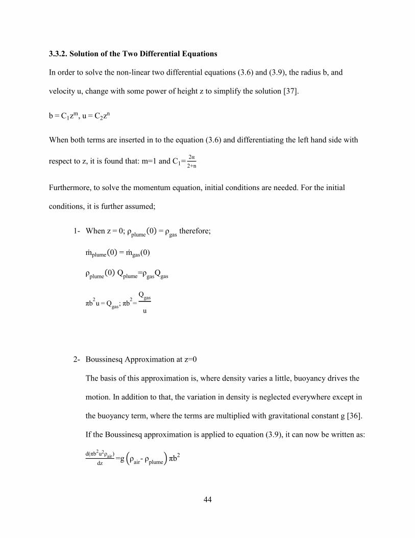
44
3.3.2. Solution of the Two Differential Equations
In order to solve the non-linear two differential equations (3.6) and (3.9), the radius b, and
velocity u, change with some power of height z to simplify the solution [37].
b = C1zm, u = C2zn
When both terms are inserted in to the equation (3.6) and differentiating the left hand side with
respect to z, it is found that: m=1 and C1=2α
2+n
Furthermore, to solve the momentum equation, initial conditions are needed. For the initial
conditions, it is further assumed;
1- When z = 0; ρplume
(0) = ρgas
therefore;
ṁplume(0) = ṁgas(0)
ρplume
(0) Qplume
=ρgas
Qgas
πb2u = Q
gas; πb
2=
Qgas
u
2- Boussinesq Approximation at z=0
The basis of this approximation is, where density varies a little, buoyancy drives the
motion. In addition to that, the variation in density is neglected everywhere except in
the buoyancy term, where the terms are multiplied with gravitational constant g [36].
If the Boussinesq approximation is applied to equation (3.9), it can now be written as:
d(πb2u2ρair)
dz=g (ρ
air- ρ
plume) πb
2

45
For the right hand side of the equation, based on initial conditions mentioned above at
height z=0, ρplume
(0)=ρgas
and above it is already found πb2=
Qgas
u , as a result
momentum equation becomes;
d(πb2u2ρair)
dz=g (ρ
air- ρ
gas)
Qgas
u (3.10)
Given equation (3.10), inserting b=C1z and u=C2zn and differentiating with respect to
height z, enables to determine the unknowns, which are:
n = -1
3 , C1 =
6α
5 and C2 = [
25 Qgas g (ρair- ρgas)
48 π ρair α2
]
(1
3)
Since all four unknowns were solved, radius, velocity, volumetric concentration and density of
the plume as a function of height z can now be expressed as:
The radius of the plume, b;
b(z) =6α
5z (3.11)
The velocity of the plume, u;
u(z) = [25 Qgas g (ρair- ρgas)
48 π ρair α2
]
(1
3)
z(−1
3) Recalling (3.1), if we insert buoyancy flux in this equation
Bgas = g Qgas
(ρ
air- ρ
gas
ρair
) we can express velocity of the plume:
u(z) = [25 Bgas
48 π α2]
(1
3)
z(-
1
3) (3.12)
The volumetric concentration:
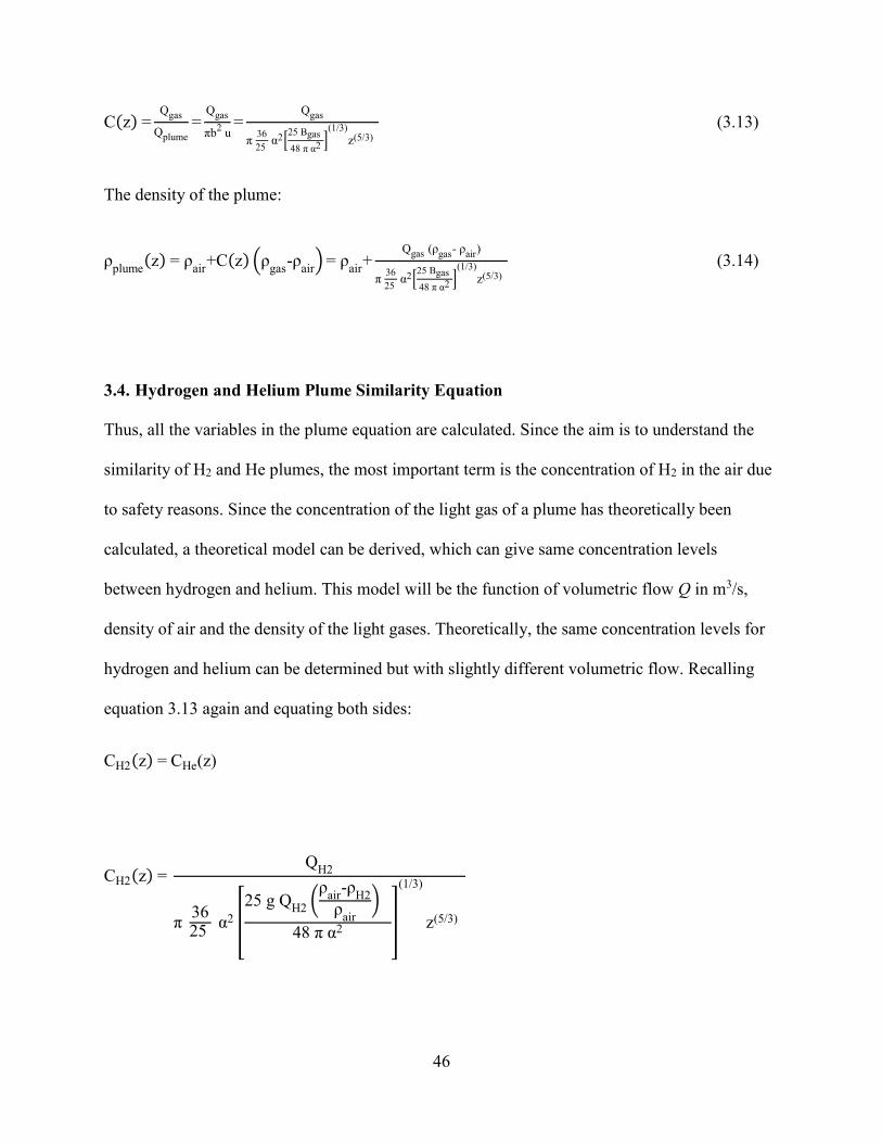
46
C(z) =Qgas
Qplume
=Qgas
πb2
u=
Qgas
π 36
25 α2[
25 Bgas
48 π α2 ](1/3)
z(5/3)
(3.13)
The density of the plume:
ρplume
(z) = ρair
+C(z) (ρgas
-ρair
) = ρair
+Qgas (ρgas- ρair)
π 36
25 α2[
25 Bgas
48 π α2 ](1/3)
z(5/3) (3.14)
3.4. Hydrogen and Helium Plume Similarity Equation
Thus, all the variables in the plume equation are calculated. Since the aim is to understand the
similarity of H2 and He plumes, the most important term is the concentration of H2 in the air due
to safety reasons. Since the concentration of the light gas of a plume has theoretically been
calculated, a theoretical model can be derived, which can give same concentration levels
between hydrogen and helium. This model will be the function of volumetric flow Q in m3/s,
density of air and the density of the light gases. Theoretically, the same concentration levels for
hydrogen and helium can be determined but with slightly different volumetric flow. Recalling
equation 3.13 again and equating both sides:
CH2(z) = CHe(z)
CH2(z) = Q
H2
π 3625
α2 [
25 g QH2
(ρ
air-ρ
H2
ρair
)
48 π α2 ]
(1/3)
z(5/3)
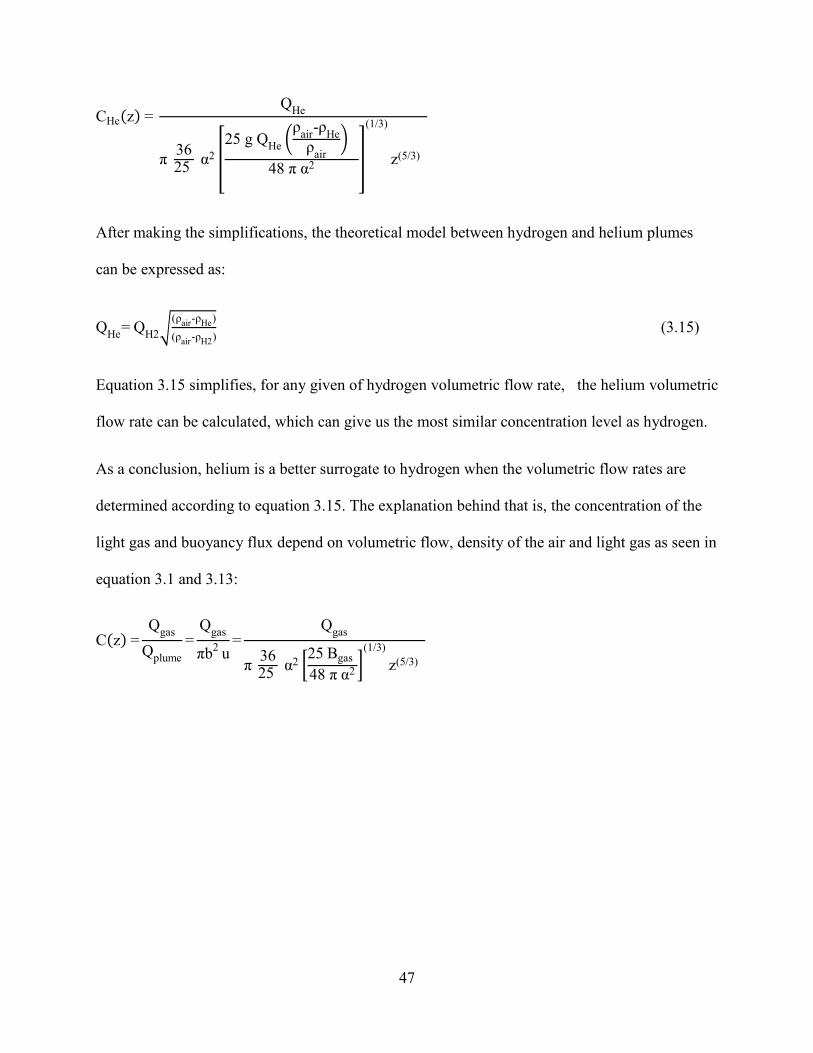
47
CHe(z) = Q
He
π 3625
α2 [
25 g QHe
(ρ
air-ρ
He
ρair
)
48 π α2 ]
(1/3)
z(5/3)
After making the simplifications, the theoretical model between hydrogen and helium plumes
can be expressed as:
QHe
= QH2√
(ρair-ρHe)
(ρair-ρH2) (3.15)
Equation 3.15 simplifies, for any given of hydrogen volumetric flow rate, the helium volumetric
flow rate can be calculated, which can give us the most similar concentration level as hydrogen.
As a conclusion, helium is a better surrogate to hydrogen when the volumetric flow rates are
determined according to equation 3.15. The explanation behind that is, the concentration of the
light gas and buoyancy flux depend on volumetric flow, density of the air and light gas as seen in
equation 3.1 and 3.13:
C(z) =Q
gas
Qplume
=Q
gas
πb2
u=
Qgas
π 3625 α2 [
25 Bgas
48 π α2 ](1/3)
z(5/3)

48
4. METHODOLOGY
4.1. Sub-Scale Residential Garage Experiment Methodology
A 1/4 sub-scale residential garage model was constructed and the experiments were conducted at
building envelope lab in Concordia University to investigate the dispersion behaviour of helium
under different cases. Sub-scale enclosure, helium supply and gas sampling system were
cautiously chosen and designed. Some results of the experiments were used to compare with
CFD predictions. Specifics of the experiment were explained in this chapter, including
experimental components, instruments, experimental methods and data acquisition.
4.1.1. Sub-scale Model
4.1.1.1. Geometry
The model used in this study is a 1/4 sub-scale model of a two car residential garage model
(Figure 4-1). The model was built with similar model geometry of sub-scale garage model used
by Prasad et al. [22]. The model was made from 6 mm thick plexiglas, for its transparency, clear
visuals were provided during the measurements.
There were three 2.6 mm × 2.6 mm vents on the top part of the model, one in the center and two
other were close to a sidewall. These vents were used to measure the effect of both natural and
mechanical ventilation. There were three 2.6 mm × 2.6 mm vents on the sidewall, which were
also used for the reason mentioned above. There were three more 3.6 mm × 3.6 mm vents on the
bottom of the model that allowed modifying the location of the helium supply. The top part of
the enclosure was independent from the rest of the model, after each test, the part was removed
in order to ventilate the model.
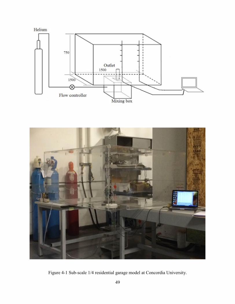
49
Figure 4-1 Sub-scale 1/4 residential garage model at Concordia University.

50
4.1.1.2. Helium Supply
Pure helium was supplied into the model to measure concentration level in different scenarios. In
the study of Prasad et al. [24], the helium supply flow rate was determined from a leakage rate of
5 kg of hydrogen into full-scale garage of 59.8m3. The corresponding hydrogen volume of 0.89
m3 for the sub-scale garage required volume flow rates of 14.8 L/min and 3.71 L/min. for 3600
and 14400 seconds release period. Therefore, for the experiments’ different scenarios; 5L/min,
10L/min and 15L/min flow rates were chosen.
The helium was supplied by a 40 liter compressed helium cylinder. A mass flow controller
(Alicat MCR-250SLPM-D/5M) (Figure 4-2) was used to fix the flow of helium at the desired
rate. The flow meter was controlled manually, desired flow rates were set from the flow
controller menu. During the experiments, ±0.3L/min from the set value was observed.
Figure 4-2 Helium mass flow controller.

51
4.1.1.3. Gas Sampling System
Gas sampling was conducted with eight XEN-5310 sensors and two USB readout XEN-85000.
Sensors measure the helium concentration by measuring the thermal conductivity of the ambient
air using a thermal conductivity gauge (Figure 4-3). To eliminate the effect of the temperature
and humidity, these values are measured separately and a correction was made by the micro
controller. Each device was factory calibrated, but before commencing the experiments, each
sensors’ measurement was controlled and checked at the lab.
Figure 4-3 XEN-5310 Helium Sensor (left) XEN-85000 USB Readout (right).
4.1.1.3.1. Calibration of Sensors
In order to conduct experiments, eight helium sensors XEN-5310 and two USB read out XEN-
85000 were recalibrated. For the calibration, previously designed mixing box was used. Figure 4-
4 represents the calibration set up for the sensors. Sensors were grouped into two and measured
at the same time. In that way, the two sensors’ results were checked in the same condition. On
the side of the mixing box, the first opening was closed and the second opening was for the
supply of the helium gas.

52
Figure 4-4 Calibration Setup for 8 sensors and 2 USB outputs.
The basic process of the calibration was, placing two sensor on the top opening, starting the
measurements of the helium concentration, waiting and observing the reaction of the sensors
before releasing the helium for 0-100 seconds and after opening the valve for the helium tank
and observing the change in the concentration level of helium in both sensors. Each sensor
comparison graphs are shown in the Appendix A. According to the manufacturer, reaction times
for the sensor are 1 second with the accuracy of 1.1%. Labview software along with H2 Polling
R232 communication software was used to acquire the output from the sensor. Digital output
was user specified, % concentration was chosen for each measurement. Figure 4-5 represents the
location of the sensors.
Figure 4-5 Location of the sensors inside the model.
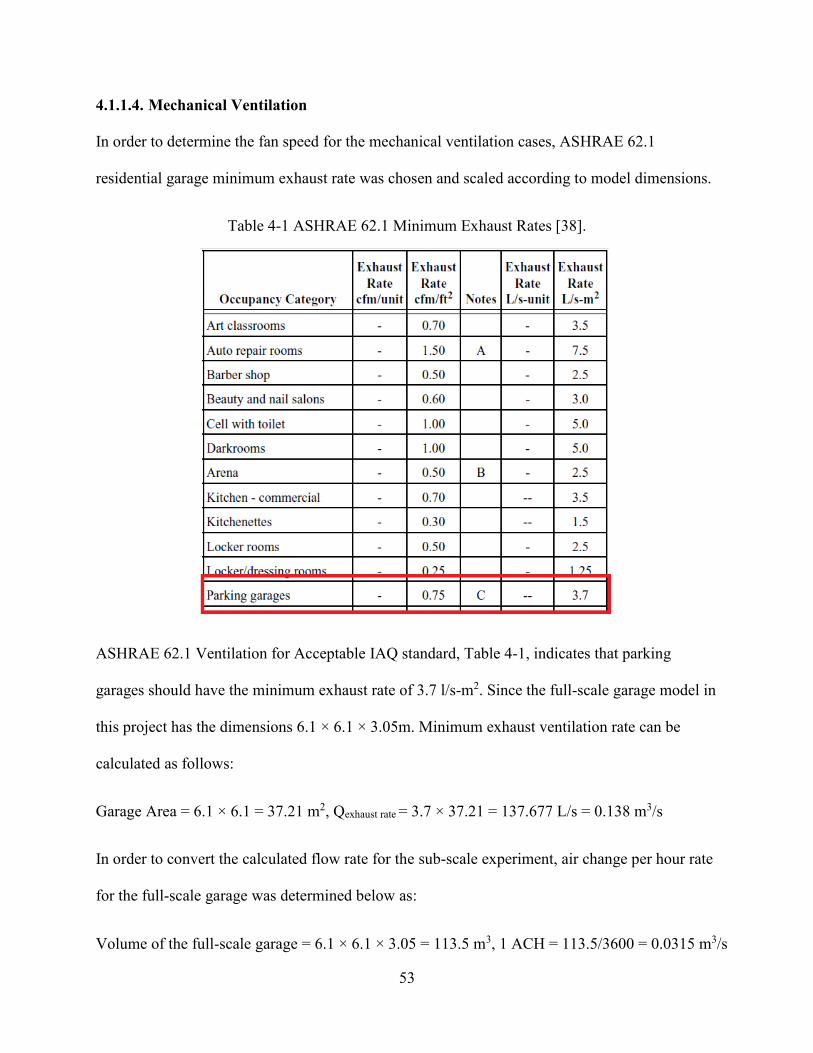
53
4.1.1.4. Mechanical Ventilation
In order to determine the fan speed for the mechanical ventilation cases, ASHRAE 62.1
residential garage minimum exhaust rate was chosen and scaled according to model dimensions.
Table 4-1 ASHRAE 62.1 Minimum Exhaust Rates [38].
ASHRAE 62.1 Ventilation for Acceptable IAQ standard, Table 4-1, indicates that parking
garages should have the minimum exhaust rate of 3.7 l/s-m2. Since the full-scale garage model in
this project has the dimensions 6.1 × 6.1 × 3.05m. Minimum exhaust ventilation rate can be
calculated as follows:
Garage Area = 6.1 × 6.1 = 37.21 m2, Qexhaust rate = 3.7 × 37.21 = 137.677 L/s = 0.138 m3/s
In order to convert the calculated flow rate for the sub-scale experiment, air change per hour rate
for the full-scale garage was determined below as:
Volume of the full-scale garage = 6.1 × 6.1 × 3.05 = 113.5 m3, 1 ACH = 113.5/3600 = 0.0315 m3/s
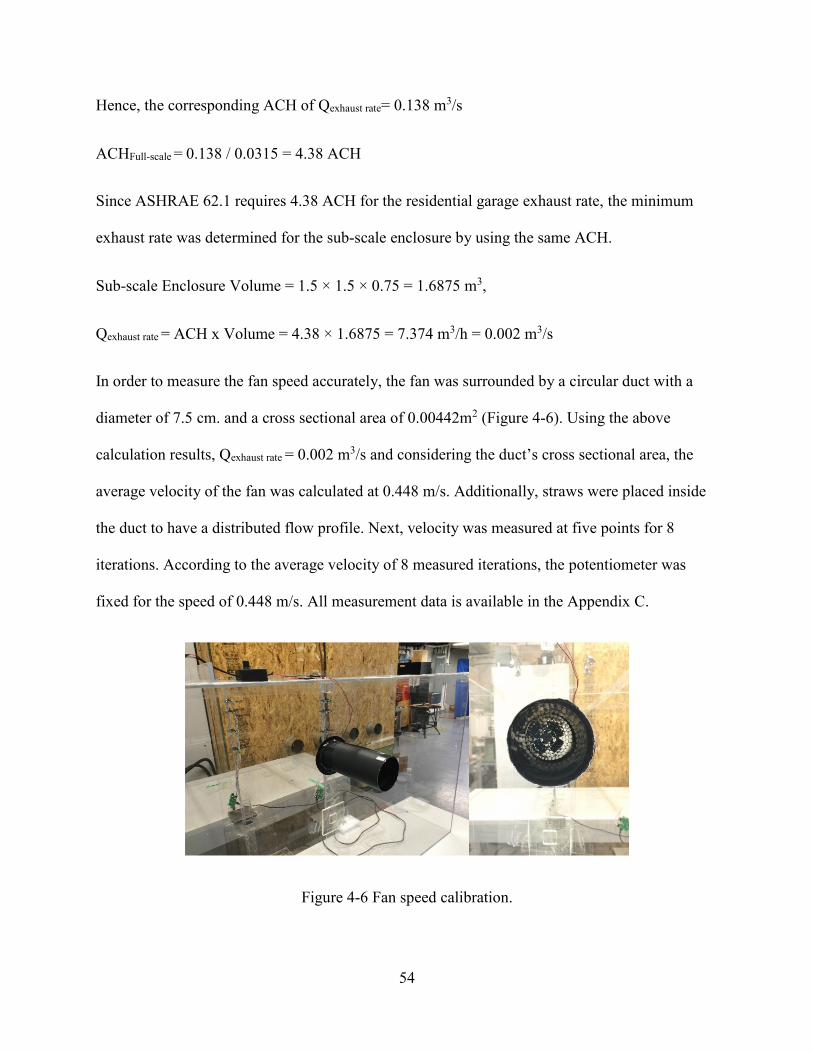
54
Hence, the corresponding ACH of Qexhaust rate= 0.138 m3/s
ACHFull-scale = 0.138 / 0.0315 = 4.38 ACH
Since ASHRAE 62.1 requires 4.38 ACH for the residential garage exhaust rate, the minimum
exhaust rate was determined for the sub-scale enclosure by using the same ACH.
Sub-scale Enclosure Volume = 1.5 × 1.5 × 0.75 = 1.6875 m3,
Qexhaust rate = ACH x Volume = 4.38 × 1.6875 = 7.374 m3/h = 0.002 m3/s
In order to measure the fan speed accurately, the fan was surrounded by a circular duct with a
diameter of 7.5 cm. and a cross sectional area of 0.00442m2 (Figure 4-6). Using the above
calculation results, Qexhaust rate = 0.002 m3/s and considering the duct’s cross sectional area, the
average velocity of the fan was calculated at 0.448 m/s. Additionally, straws were placed inside
the duct to have a distributed flow profile. Next, velocity was measured at five points for 8
iterations. According to the average velocity of 8 measured iterations, the potentiometer was
fixed for the speed of 0.448 m/s. All measurement data is available in the Appendix C.
Figure 4-6 Fan speed calibration.
55
4.1.2. Experimental Method
An experimental method was used to examine the effects of natural and mechanical ventilation
on the concentration levels of helium in a sub-scaled residential garage model. Moreover,
similarities between helium and hydrogen plumes were also observed for future experiments.
Important parameters for the experiments are as follows:
Natural ventilation
Volumetric flow rate
Release location
Injector height
Release direction
Release time
Mechanical Ventilation
ASHRAE 62.1 minimum residential garage exhaust rate
Furthermore, the new model between hydrogen and helium plumes discussed in section 3, were
observed in line with the simulation predictions.
4.1.2.1. Series of Tests
In this section, helium concentration measurement for 20 different cases are indicated. Table 4-2
below shows the details of the cases. See Appendix B for the measurements of 20 different cases.

56
Table 4-2 Experimental cases.
QHe
(lt/min) Vents
Release Time
(min)
Injector
Location&Height
Injection
Direction Type
Case 1 15 - 5 Center, 12.3cm Up Natural ventilation
Case 2 15 2 (Ceiling center,
side wall up) 30
Corner(18-37cm),
12.3 cm Up Natural ventilation
Case 3 5 1 (Side wall up) 30 Center, 12.3cm Up Natural ventilation
Case 4 10 1 (Side wall up) 30 Center, 12.3cm Up Natural ventilation
Case 5 15 1 (Side wall up) 30 Center, 12.3cm Up Natural ventilation
Case 6 15 2 (Ceiling center,
side wall up) 30 Center, 12.3cm Down Natural ventilation
Case 7 10 1 (Side wall up) 5 Center, 12.3cm Up Natural ventilation
Case 8 10 1 (Side wall up) 15 Center, 12.3cm Up Natural ventilation
Case 9 10 1 (Side wall up) 30 Center, 12.3cm Up Natural ventilation
Case 10 10 1 (Side wall up) 45 Center, 12.3cm Up Natural ventilation
Case 11 15 1 (Ceiling Centre) 5 Center, 12.3cm Up Natural ventilation
Case 12 15 1 (Ceiling Centre) 20 Center, 12.3cm Up Natural ventilation
Case 13 15 1 (Side wall up) 30 Center, 55 cm Up Natural ventilation
Case 14 15 2 (Ceiling center,
side wall up) 5 Center, 12.3cm Up Natural ventilation
Case 15 15 2 (Ceiling center,
side wall up) 45 Center, 12.3cm Up Natural ventilation
Case 16 15 2 (Side wall up,
side wall center) 5 Center, 12.3cm Up Natural ventilation
Case 17 15 2 (Side wall up,
side wall center) 45 Center, 12.3cm Up Natural ventilation
Case 18 15 2 (Ceiling, beside
wall) 5 Center, 12.3cm Up Natural ventilation
Case 19 15 2 (Ceiling, beside
wall) 45 Center, 12.3cm Up Natural ventilation
Case 20 15 1 (Ceiling Center) 20 Center, 12.3cm Up Mechanical ventilation
(Fan= Side wall up)

57
4.1.2.2. Experimental Procedure
Lab safety requirements were followed for each 20 case’s experimental procedure. Cases 1-19
were conducted with only natural ventilation, whereas case 20 was conducted with mechanical
ventilation. For every case, helium concentrations were measured from 8 sensors, where 4
sensors were placed inside (center) of the plume and remaining 4 were placed 40 cm away from
two side walls, as shown in Figure 4-5.
The experimental procedures are:
1. Remove top of the experiment model and check the sensor for helium concentration level
inside the model.
2. Use the air pump to extract the helium inside the mixing;
3. Wait until helium concentration level are less than 0.05% for each sensor;
4. Seal the top of the model and necessary vents with a duct tape and other apparatus;
5. Check the 8 sensors’ connection to the laptop, start the H2 Polling R232 communication
software, check the display for both sensor’s measurements;
6. Turn on the mass flow meter, set the desired flow rate manually;
7. Open the regulator valve of helium tank and start the test;
8. Check the software output for concentration level and the graphs;
9. Measure the flow direction and speed through vents;
10. Save the data and turn of the mass flow meter and helium tank regulator respectively.
For cases 1-19 above procedure steps were followed. For mechanical ventilation case 20
abovementioned steps were also followed. Additionally, calibration of the fan speed was
conducted before step 5.

58
5. RESULTS AND DISCUSSION
5.1. Sub-Scale Residential Garage Tests
The results of the experiments, conducted at Concordia University Building Envelope Lab are
subsequently presented in this chapter. Natural ventilation and mechanical ventilation cases are
discussed by the measured helium concentrations. The graphs that will be shown in this section
only contain 4 sensor data, in 20 cases, it was observed that maximum helium concentration
inside the plume was measured at sensor E1 (h=0.4m) and minimum concentration was
measured at sensor E4 (h=0.65m), whereas outside the plume, maximum helium concentration
measured at sensor ED (h=0.65m) and minimum concentration measured at sensor EA (h=0.4m).
Eight sensors’ measured data can be found for 20 cases in Appendix B.
5.1.1. Natural Ventilation Cases
5.1.1.1. Volumetric Flow Rate
As described in Chapter 4 – Helium Supply, leakage rates from a 5 kg hydrogen tank of a fuel
cell into a residential garage were determined and scaled to the model for 1 hour and 4 hour
releases, which were 14.8L/min and 3.71L/min respectively [24].
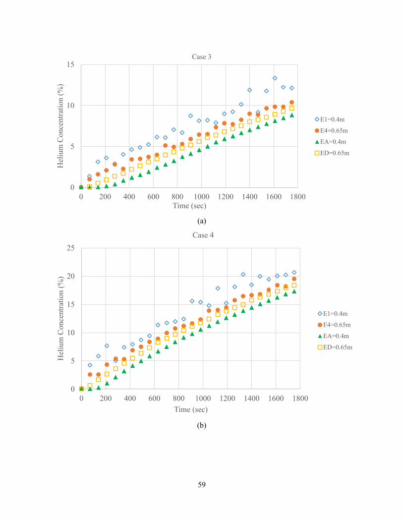
59
(a)
(b)
0
5
10
15
0 200 400 600 800 1000 1200 1400 1600 1800
Hel
ium
Conce
ntr
atio
n (
%)
Time (sec)
Case 3
E1=0.4m
E4=0.65m
EA=0.4m
ED=0.65m
0
5
10
15
20
25
0 200 400 600 800 1000 1200 1400 1600 1800
Hel
ium
Conce
ntr
atio
n (
%)
Time (sec)
Case 4
E1=0.4m
E4=0.65m
EA=0.4m
ED=0.65m

60
(c)
Figure 5-1 Comparison for different volume flow rates (a) 5L/min (b) 10L/min and (c) 15L/min
The effects of different flow rates 5L/min, 10L/min and 15L/min corresponding to Case 3, Case
4 and Case 5 respectively, are shown in Figure 5-1 (Details of all cases are listed at Table 4-2).
At the end of 1800 seconds, the maximum concentration level for Case 3 is 12-14%, for Case 4
is 20-23% and for Case 5 it is between 27-30%. At the end of 1800 seconds, the maximum
helium concentration in Case 3 (5L/min) is lower than hydrogen explosion limit 18.3-59%
(Table 1-2) whereas, Case 4’s (10L/min) and Case 5’s (15L/min) maximum concentrations are
higher than the lower hydrogen explosion limit.
0
5
10
15
20
25
30
0 200 400 600 800 1000 1200 1400 1600 1800
Hel
ium
Conce
ntr
atio
n (
%)
Time (sec)
Case 5
E1=0.4m
E4=0.65m
EA=0.4m
ED=0.65m

61
5.1.1.2. Release Location
In order to observe the effect of different release location on concentration levels of helium, the
injector was not located to the center of the base but at 18 cm away from the sidewall with the
vent and 37 cm away from the side wall without the vent as shown in Figure 5-2.
Figure 5-2 Location of the helium sensors and injector for Case 2.

62
(a)
(b)
Figure 5-3 Comparison for different release locations (a) Corner release (b) Center release.
0
5
10
15
20
25
30
0 200 400 600 800 1000 1200 1400 1600 1800
Hel
ium
Conce
ntr
atio
n (
%)
Time (sec)
Case 2
E1=0.4m
E4=0.65m
EA=0.4m
ED=0.65m
0
5
10
15
20
25
30
0 200 400 600 800 1000 1200 1400 1600 1800
Hel
ium
Conce
ntr
atio
n (
%)
Time (sec)
Case 15
E1=0.4m
E4=0.65m
EA=0.4m
ED=0.65m

63
In case 15, the injector was located at the center. In both cases sensors 1, 2, 3 and 4 were located
inside the plume, above the injector and helium gas was supplied 15L/min for 1800 seconds,
until the helium concentration level reached 30% (most easily ignited in air limit for hydrogen).
Sensors A, B, C, and D were located 0.4 m away from the walls. Figure 5-3 represents the
concentration levels of helium in 1800 seconds for both cases. The maximum concentration for
Case 2 and Case 15 is around 30% and the two graphs have similar trends in terms of
concentration. It can be observed that the corner release does not have much influence on the
helium concentration levels inside the enclosure compared to the center release. In both cases,
maximum concentration levels exceeds hydrogen explosion limits as well as the stoichiometric
mixture limit (most easily ignited in air), which is 29% at the end of 1800 seconds.
5.1.1.3. Injector Height
In all cases the injector was located 12.3 cm above the base however, for Case 13, in order to
observe the effect of the release height, the injector was raised to 55cm, as shown in Figure 5-4.
Figure 5-4 Sensor and helium injector locations for Case 13.

64
(a)
(b)
Figure 5-5 Comparison for different release heights (a) 0.55m (b) 0.123m.
0
5
10
15
20
25
30
35
40
45
0 200 400 600 800 1000 1200 1400 1600 1800
Hel
ium
Conce
ntr
atio
n (
%)
Time (sec)
Case 13
E1=0.4m
E4=0.65m
EA=0.4m
ED=0.65m
0
5
10
15
20
25
30
35
0 200 400 600 800 1000 1200 1400 1600 1800
Hel
ium
Conce
ntr
atio
n (
%)
Time (sec)
Case 5
E1=0.4m
E4=0.65m
EA=0.4m
ED=0.65m

65
Helium volumetric flow rate, release time, vent size and vent location are exactly same for Case
5 and 13 whereas, sensor locations and helium release heights are different. The higher injector
height (0.55m) caused less mixing between air and helium, compared to the lower injector height
(0.123). The differences in concentration levels had significant between two cases as shown in
Figure 5-5. With lower injector height, helium gas rose through the top of the model with
buoyancy force and mixed with air, whereas with higher injector height, helium gas reached to
the top of the model quickly with the less mixing with air. Since the injector height for Case 13 is
0.55m, the helium concentration inside the plume was not measured. All the helium sensors were
located outside the plume.

66
(a)
(b)
Figure 5-6 Comparison for different release directions (a) Upwards (b) Downwards.
Even though both cases have the same helium volumetric flow rate, the maximum concentration
for Case 13 is close to 40%, whereas for Case 5, it is 25-30%. Therefore, in both cases, the
0
5
10
15
20
25
0 200 400 600 800 1000 1200 1400 1600 1800
Hel
ium
Conce
ntr
atio
n (
%)
Time (sec)
Case 6
E1=0.4m
E4=0.65m
EA=0.4m
ED=0.65m
0
5
10
15
20
25
30
0 200 400 600 800 1000 1200 1400 1600 1800
Hel
ium
Conce
ntr
atio
n (
%)
Time (sec)
Case 15
E1=0.4m
E4=0.65m
EA=0.4m
ED=0.65m

67
maximum helium concentration is higher than the lower hydrogen explosion limit and the most
easily ignited in air limit at the end of 1800 seconds.
Furthermore, with the lower injection point, helium gas rose towards the ceiling due to the
buoyancy force, mixed with air and caused a homogeneous distribution inside the chamber. By
contrast, with the higher injection point, helium gas aggregated on the top of the enclosure and
less mixing occurred with air causing high concentration levels of helium on the top part of the
chamber, which can describe the difference between the maximum helium concentration levels
for Case 5 and 13.
5.1.1.4. Release Direction
Figure 5-6 represents the difference between upwards and downwards release direction. Both
Case 6 and Case 15 had the exact same vent size, vent location, helium volumetric flow rate with
1800 seconds of helium injection. The only difference was Case 6 had downward flow direction
whereas Case 15 had upward direction. It was observed that the maximum concentration level
for Case 6 reached 20-22% and for Case 15, it reached around 30% at the end of 1800 seconds.
In both cases, maximum helium concentrations were above the minimum hydrogen explosion
limit but Case 6’s maximum concentration was below the stoichiometric mixture limit.
Moreover, in Case 6 less fluctuations for concentration levels can be observed. The reason for
the less fluctuations can be explained by the helium gas exited upside down through the injector,
with gravity, a turnover occurred and the gas started to rise towards ceiling with buoyant force.
This gravitational resistance created more homogeneous mixture inside the chamber and resulted
in lower concentration levels compared to upward release scenario.

68
5.1.1.5. Gas Release Time
(a)
(b)
0
2
4
6
8
10
12
0 50 100 150 200 250 300
Hel
ium
Conce
ntr
atio
n (
%)
Time (sec)
Case 7
E1=0.4m
E4=0.65m
EA=0.4m
ED=0.65m
0
5
10
15
20
0 100 200 300 400 500 600 700 800 900
Hel
ium
Conce
ntr
atio
n (
%)
Time (sec)
Case 8
E1=0.4m
E4=0.65m
EA=0.4m
ED=0.65m
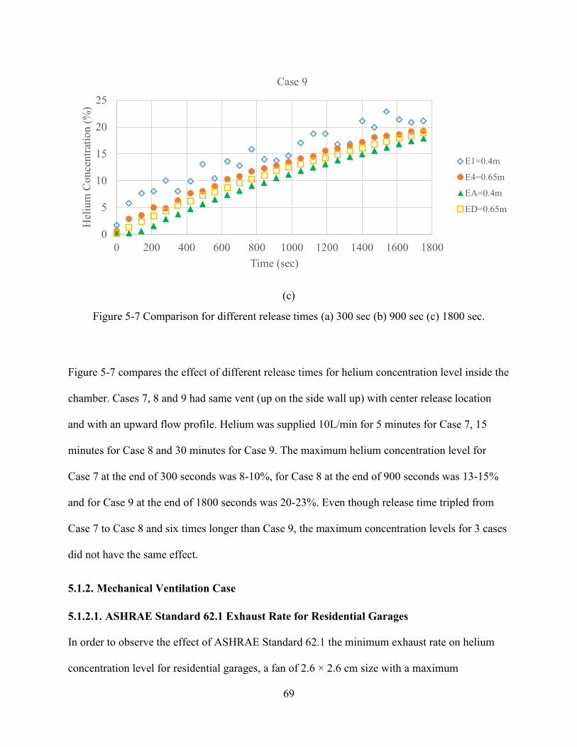
69
(c)
Figure 5-7 Comparison for different release times (a) 300 sec (b) 900 sec (c) 1800 sec.
Figure 5-7 compares the effect of different release times for helium concentration level inside the
chamber. Cases 7, 8 and 9 had same vent (up on the side wall up) with center release location
and with an upward flow profile. Helium was supplied 10L/min for 5 minutes for Case 7, 15
minutes for Case 8 and 30 minutes for Case 9. The maximum helium concentration level for
Case 7 at the end of 300 seconds was 8-10%, for Case 8 at the end of 900 seconds was 13-15%
and for Case 9 at the end of 1800 seconds was 20-23%. Even though release time tripled from
Case 7 to Case 8 and six times longer than Case 9, the maximum concentration levels for 3 cases
did not have the same effect.
5.1.2. Mechanical Ventilation Case
5.1.2.1. ASHRAE Standard 62.1 Exhaust Rate for Residential Garages
In order to observe the effect of ASHRAE Standard 62.1 the minimum exhaust rate on helium
concentration level for residential garages, a fan of 2.6 × 2.6 cm size with a maximum
0
5
10
15
20
25
0 200 400 600 800 1000 1200 1400 1600 1800
Hel
ium
Con
centr
atio
n (
%)
Time (sec)
Case 9
E1=0.4m
E4=0.65m
EA=0.4m
ED=0.65m

70
volumetric flow rate of 0.002 m3/s was used for the sub-scale model. Fan speed determination,
scaling for experimental model and fan speed calibration was explained in Chapter 4. In Figure
5-8, Case 20 shows the mechanical ventilation experiment with the ceiling center vent and the
fan location on the upper sidewall vent whereas, Case 12 shows the natural ventilation case with
only a ceiling center vent.
Due to the fan’s turbulence effect, helium concentration levels inside the plume fluctuates for the
sensors E1 and E4. For 1200 seconds, maximum helium concentration level in both cases are 20-
23%, which is higher than the hydrogen explosion limit.
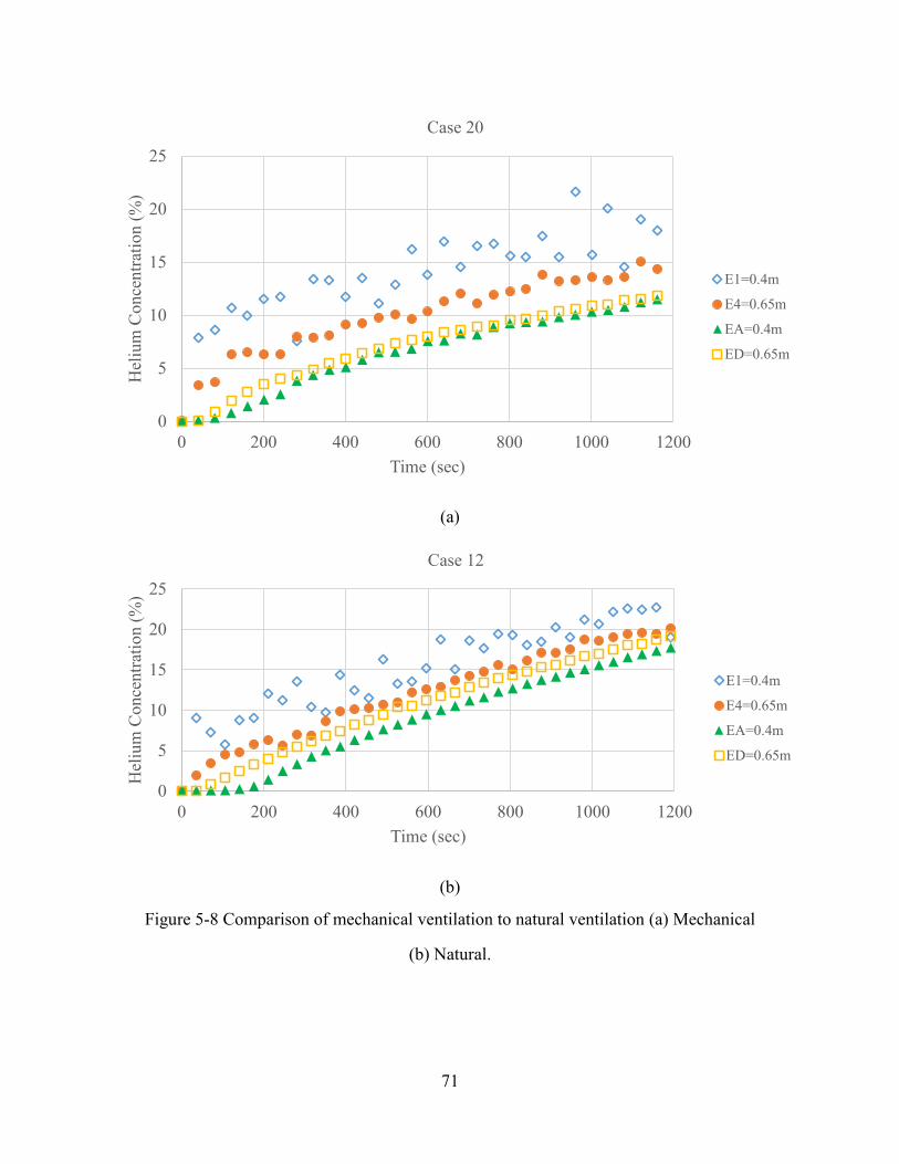
71
(a)
(b)
Figure 5-8 Comparison of mechanical ventilation to natural ventilation (a) Mechanical
(b) Natural.
0
5
10
15
20
25
0 200 400 600 800 1000 1200
Hel
ium
Conce
ntr
atio
n (
%)
Time (sec)
Case 20
E1=0.4m
E4=0.65m
EA=0.4m
ED=0.65m
0
5
10
15
20
25
0 200 400 600 800 1000 1200
Hel
ium
Conce
ntr
atio
n (
%)
Time (sec)
Case 12
E1=0.4m
E4=0.65m
EA=0.4m
ED=0.65m

72
On the other hand, for the sensors outside the plume; EA and ED, the maximum helium
concentration level is 11-12% for Case 20 whereas, 18-19% for Case 12. The reason for this
difference between two cases was the influence of the exhaust fan. Outside the plume, the
maximum helium concentration level for Case 20 was below the lower hydrogen explosion limit,
but without the fan, for Case 12, it is close to the point for the lower hydrogen explosion limit.
CFD Comparison of Hydrogen and Helium Plume Similarity
5.1.3. CFD Model
CFD modeling was used to simulate helium and hydrogen plumes and investigate their
similarity. Since conducting the experiments with hydrogen is not safe, ANSYS Fluent14.5 CFD
software allowed us to observe the plume similarity and compare same volumetric flow and the
Equation 3.15, which was derived in Chapter 3. For the simulation model, the Large Eddy
Simulation (LES) turbulence model was chosen. For the transient cases, Giannissi et al. [35]
concluded that the LES model had compliance with the experiment results as mentioned in
Chapter 2.
5.1.3.1. Geometry
The geometry of the model was designed exactly same as the sub-scale experimental chamber at
Concordia University Building Envelope Lab (Figure 5-9). The simulation was conducted under
the exact conditions with Case 15, as indicated in Chapter 4.
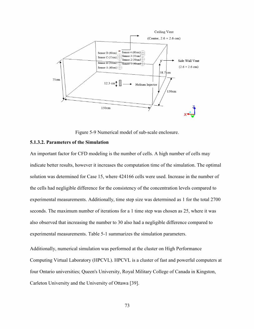
73
Figure 5-9 Numerical model of sub-scale enclosure.
5.1.3.2. Parameters of the Simulation
An important factor for CFD modeling is the number of cells. A high number of cells may
indicate better results, however it increases the computation time of the simulation. The optimal
solution was determined for Case 15, where 424166 cells were used. Increase in the number of
the cells had negligible difference for the consistency of the concentration levels compared to
experimental measurements. Additionally, time step size was determined as 1 for the total 2700
seconds. The maximum number of iterations for a 1 time step was chosen as 25, where it was
also observed that increasing the number to 30 also had a negligible difference compared to
experimental measurements. Table 5-1 summarizes the simulation parameters.
Additionally, numerical simulation was performed at the cluster on High Performance
Computing Virtual Laboratory (HPCVL). HPCVL is a cluster of fast and powerful computers at
four Ontario universities; Queen's University, Royal Military College of Canada in Kingston,
Carleton University and the University of Ottawa [39].

74
Table 5-1 Simulation parameters.
Sub-Scale Size 1.5 m (L) × 1.5 m (W) × 0.75 m (H)
Vent Size 0.026 m × 0.026 m
Vent Location 1 side wall, 1 ceiling center
Injector Size 0.036 × 0.036 m
Injector Height 0.123 m
Injector Location Center of the base
Concentration Sensors 8 Sensors (4 Inside, 4 Outside the plume)
Location of the Sensors 4 Inside = Center 4 Outside = 0.4 m away from walls
Boundary Conditions Ceiling Vent:
Pressure Outlet (0)
Side Wall Vent:
Velocity Inlet (m/s)
Injector:
Mass flow inlet
(kg/s)
Number of Cells 424166
Simulation Time 2700 seconds
Computation Time 5 h 30 min
The initial temperature of released helium and air temperature in the chamber were set equal to
the specified in experimental data and initial pressure of the model was set to 101325 Pa. Initial
velocities were set to zero in the whole computational domain. The boundary conditions for the
injector was set as the mass flow inlet and the ceiling vent was set as pressure outlet, where the
gauge pressure was equal to zero. For the sidewall vent, the velocity inlet was chosen during the
experimental phase for Case 15, the velocity was measured through the five points of the vent (4
corners and 1 center) and the velocity magnitude was set for the simulation as the average of
these measurements. Figure 5-10 shows the predicted profile of helium concentration at the end
of 2700 seconds.
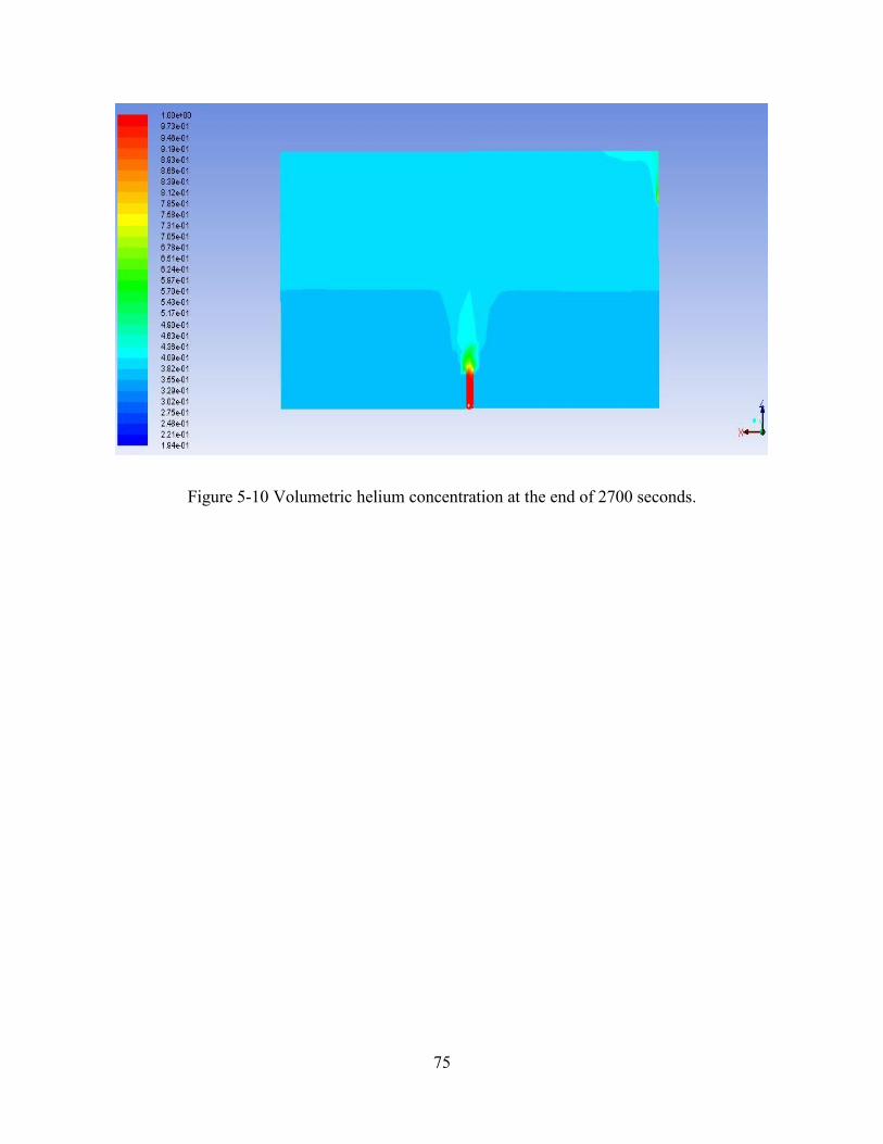
75
Figure 5-10 Volumetric helium concentration at the end of 2700 seconds.

76
5.1.4. Comparison of CFD Predictions to Experimental Data
5.1.4.1. Helium Concentrations
Figure 5-11 Comparison of predicted helium concentrations to measured data for Case 15.
Figure 5-11 shows the comparison of helium concentration levels for the CFD predictions (lines)
and experiment measurements (dots). Visually the CFD predictions are in good agreement with
experimental measurements however, in first 300 seconds, measured and predicted values
fluctuate due to the initial spatial behavior of helium gas. Table 5-3 shows the average
percentage accuracy of CFD predictions to experimental measurements for the four sensors
inside the plume between 300 seconds to 2700 seconds. Simulation results have a tendency to
0
5
10
15
20
25
30
35
40
0 300 600 900 1200 1500 1800 2100 2400 2700
Hel
ium
Conce
ntr
atio
n (
%)
Time (sec)
Case 15
S1=0.4m (Simulation) S2=0.5m (Simulation) S3=0.6m (Simulation) S4=0.65m (Simulation)
E1=0.4m (Experiment) E2=0.5m (Experiment) E3=0.55m (Experiment) E4=0.65m (Experiment)

77
overestimate the measured helium concentrations in the first 300 seconds and underestimate
between 300 seconds to 2700 seconds. In order to improve the results, especially for the first 300
seconds, further experimental data and CFD modeling is needed.
5.1.5. Comparison for Hydrogen and Helium Plume Similarity Using the CFD Model
In previous hydrogen studies, due to safety issues, helium was used as a surrogate with the same
volumetric flow rate, lacking a theoretical model between the two gases. In Chapter 3, a new
theoretical model was derived, equation 3.15, which enables to determine flow rates of two gases
so that similar plumes can be achieved in terms of concentration levels. Table 5-2 shows the
determined hydrogen and helium flow rates that were used in the CFD comparison for Case 15.
Table 5-2 Hydrogen and helium volumetric flow rates for simulations.
Model between hydrogen
and helium volumetric flow rates
Helium Flow Rate
(L/min)
Hydrogen Flow Rate
(L/min)
QHe
= QH2
15 15
QHe
= QH2
√(ρ
air-ρ
He)
(ρair
-ρH2
) 15 15.5955
5.1.5.1. Same Volumetric Flow for Hydrogen and Helium
Figure 5-12 represents the comparison of the simulation predictions of the same volumetric flow
for both hydrogen and helium gases, which was set to 15L/min. When the same volumetric flow
was used, predictions of the helium concentration levels were close with the hydrogen
concentration levels. However, differences could be observed inside the plume, which is the
most critical domain for the safety issues. In Table 5-3, average percentage accuracies were
listed for the similarity of hydrogen and helium plumes.
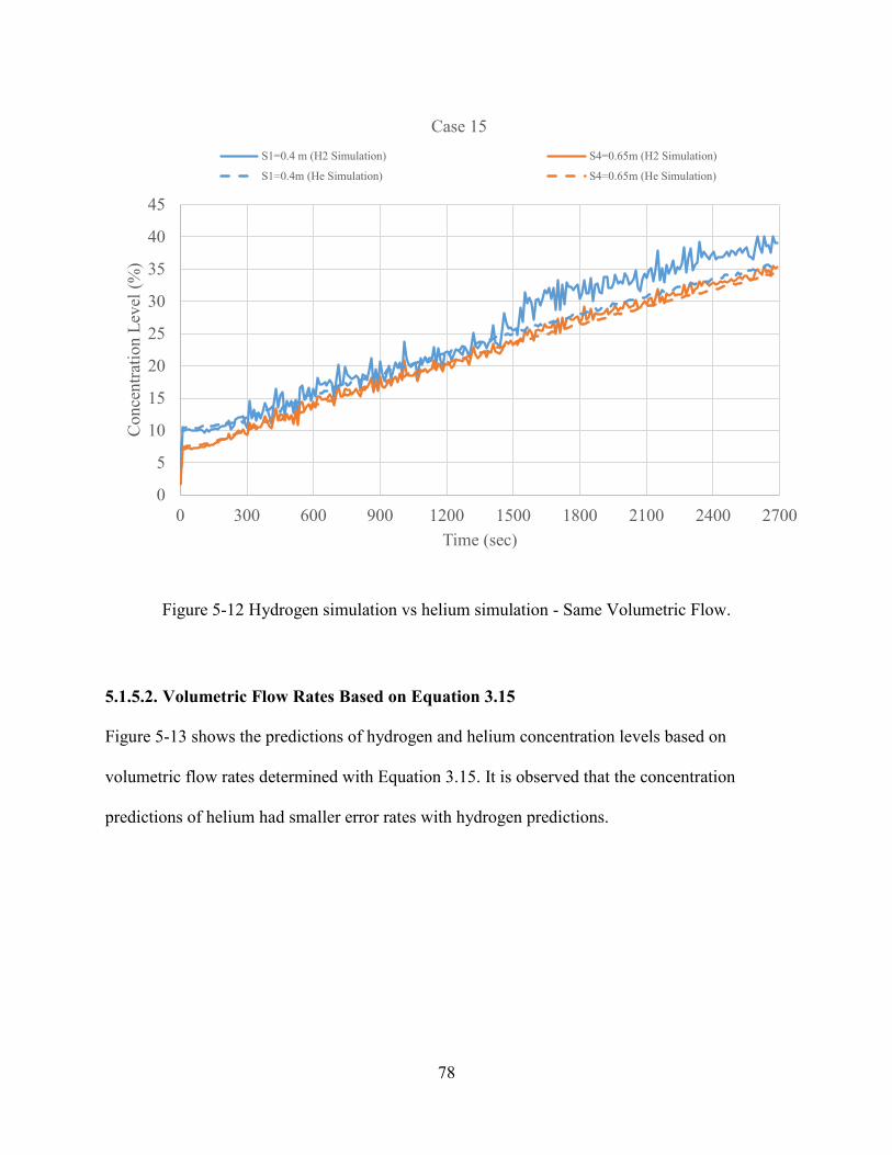
78
Figure 5-12 Hydrogen simulation vs helium simulation - Same Volumetric Flow.
5.1.5.2. Volumetric Flow Rates Based on Equation 3.15
Figure 5-13 shows the predictions of hydrogen and helium concentration levels based on
volumetric flow rates determined with Equation 3.15. It is observed that the concentration
predictions of helium had smaller error rates with hydrogen predictions.
0
5
10
15
20
25
30
35
40
45
0 300 600 900 1200 1500 1800 2100 2400 2700
Conce
ntr
atio
n L
evel
(%
)
Time (sec)
Case 15
S1=0.4 m (H2 Simulation) S4=0.65m (H2 Simulation)
S1=0.4m (He Simulation) S4=0.65m (He Simulation)

79
Figure 5-13 Hydrogen simulation vs helium simulation – Equation 3.15.
Table 5-3 Percentage accuracy for Case 15.
Case 15 Helium Experiment vs
Helium Simulation
Hydrogen Simulation vs
Helium Simulation
Same Volumetric Flow
Hydrogen Simulation vs
Helium Simulation
Equation 3.15
Sensor 1 6.14% 7.60% 5.63%
Sensor 2 4.47% 5.30% 4.33%
Sensor 3 4.21% 3.84% 3.49%
Sensor 4 4.89% 3.32% 3.17%
5.2. Summary
This chapter investigates the effects of natural and mechanical ventilation by measuring the
helium concentration levels inside the sub-scale chamber. Additionally, a CFD model was used
0
5
10
15
20
25
30
35
40
0 300 600 900 1200 1500 1800 2100 2400 2700
Con
centr
atio
n L
evel
Time (sec)
Case 15
S1=0.4 m (H2 Simulation) S4=0.65m (H2 Simulation)
S1=0.4m (He Simulation) S4=0.65m (He Simulation)

80
to compare how hydrogen and helium plumes were similar in terms of concentration level with
using the same volumetric flow rate and Equation 3.15, which was derived in Chapter 3.
In the natural ventilation cases section, the effect of different volumetric flow rates, release
locations, injector heights, release directions and release times were compared for helium
concentration levels inside the chamber. It was found that the volumetric flow rate had a
significant effect on helium concentration levels, whereas different release location had not
critical effect. On the other hand, higher injector height had greater helium concentration
compared to the case with the lower injector height due to the higher mixing potential of the
lower injection point. Additionally, the downward release direction had significant effect
compared to the upward release direction due to the gravitational and buoyancy forces. Finally,
release times also had noticeable effect on helium concentration inside the chamber.
For the mechanical ventilation case, due to the effect of forced ventilation, high fluctuations
were observed at the sensors inside the plume and the maximum concentration levels did not
have a significant difference inside the plume compared to the same natural ventilation case. On
the other hand, differences were observed outside the plume, the maximum concentration level
dropped 7% and caused the level to stay below the lower explosion limit.
Additionally, results from the sub-scale experiment measurements were used to verify the
simulation model in terms of helium concentrations. In order to investigate the hydrogen and
helium plume similarity, the same model was used to compare the effects of same volumetric
flow with the equation 3.15. Matching concentrations were found for both flows outside the
plume whereas, inside the plume, which is more critical in terms of safety issues, Equation 3.15
had smaller error rates for helium concentration levels while predicting the hydrogen
concentrations.

81
6. CONCLUSION AND FUTURE WORK
This thesis proposed a new theoretical model between hydrogen and helium plumes for the
safety analysis of hydrogen fuel cell technology’s residential applications. The study included a
complete literature review of three different sub-scaled tests of helium dispersion in an
enclosure. In addition, sub-scaled experiments were conducted to understand the dispersion
behaviour of helium during a leakage under the effect of natural and mechanical ventilations.
6.1. Conclusion
One of the promising alternative energy source to power residential homes in near future is
hydrogen fuel cell technology. However, in case of a hydrogen gas leakage, it is extremely
dangerous and flammable with in the concentration limits of 4-74% in air. In order to overcome
this safety issue, scientist conducted many sub-scale and full scale experiments along with CFD
simulations to investigate the dispersion behavior of the hydrogen. The detailed literature review
showed that helium can be used as a surrogate to hydrogen. Experiment results showed that mass
flow rate, leak location and having two vents; near the top and bottom of the wall had significant
effect, whereas release location, vent size had weak effect on helium concentrations inside the
enclosure.
On the other hand, it has also been found that there are differences between hydrogen and helium
concentrations before the plumes becomes stable, during the initial release of the gases. Until
now, the similarity of the plumes between two gases only rely on experimental results, without a
theoretical model. Equation 3.15 derived in this study describes that for any given of hydrogen
volumetric flow rate, the helium volumetric flow rate can be calculated, which can give smaller
error rates for concentration level as hydrogen.

82
Additionally, in this study, series of experiments were conducted to observe the effects of natural
and mechanical ventilation by measuring the helium concentration levels inside the 1/4 sub-scale
residential garage model. In the natural ventilation cases, the effect of different volumetric flow
rates, release locations, injector heights, release directions and release times were compared for
helium concentration levels inside the chamber. It was found that the volumetric flow rate,
higher injector height, release times and downward release direction had significant effects on
helium concentration levels, whereas different release location had not critical effect. For the
mechanical ventilation case, the maximum concentration levels did not have a significant
difference inside the plume compared to the same natural ventilation case. However, differences
were observed outside the plume, the maximum concentration level dropped and caused the level
to stay below the lower explosion limit.
Finally, a CFD model was used to compare how hydrogen and helium plumes were similar in
terms of concentration level with using the same volumetric flow rate and Equation 3.15. Results
from the sub-scale experiment measurements were used to verify the simulation model in terms
of helium concentrations. In order to investigate the hydrogen and helium plume similarity, the
same model was used to compare the effects of same volumetric flow with the equation 3.15.
Matching concentrations were found for both flows outside the plume whereas, inside the plume,
which is more critical in terms of safety issues, Equation 3.15 had smaller error rates for helium
concentration levels while predicting the hydrogen concentrations.
6.2. Future Work
Series of experiments were conducted to determine the spatial behaviour of helium in case of a
leakage. Different scenarios for natural and mechanical ventilation cases were observed.
However, all the cases had simple enclosure geometries; obstacles, doors and equipment in the

83
residential garage were not considered. Additionally, temperature and velocity of the gas were
also not measured. More experiments are needed in the future to determine the velocity profiles
of the gas by using Time-Resolved Particle Image Velocimetry (TR-PIV). These measurements
will allow for a better understanding of helium and hydrogen dispersion during an unexpected
release.
Hydrogen and helium plume similarity is crucial for the safety of hydrogen fuel cell technology.
Air density, gravitational acceleration constant and the densities of the two gases are the
functions of buoyancy flux. Plume theory and the model for volumetric flow rates between
hydrogen and helium presented in this study were developed under steady state conditions. More
theoretical studies are needed in the future for changing temperature and transient cases.
Finally, more numerical simulations should be done to observe the effect of hydrogen dispersion
in complex geometries. Velocity of the gas and temperature of the enclosure need to be taken
into consideration for the future numerical simulations. With the support from the complex
geometry experimental results, numerical predictions can be further improved and will assist to
create a reliable hydrogen safety guide.

84
REFERENCES
[1] Sharaf, O. Z., & Orhan, M. F. (2014). An Overview of Fuel Cell Technology: Fundamentals
and Applications. Renewable and Sustainable Energy Reviews 32, 810-853.
[2] U.S. Department of Energy (2004). Module 1 - Permitting Stationary Fuel Cell Installations.
[3] EG&G Technical Services Inc. (2004). Fuel Cell Handbook (Seventh Edition). West
Virginia: U.S. Department of Energy Office of Fossil Energy.
[4] Cetin, E., Yilanci, A., Ozturk, H. K., Kasikci, I., Colak, M., & Icli, S. (2011). Construction of
a Fuel Cell System with DC Power Distribution for Residential Applications.
International Journal of Hydrogen Energy 36, 11474-11479.
[5] Cetinkaya, E., Dincer, I., & Naterer, G. (2011). Life Cycle Assessment of Various Hydrogen
Production Methods. International Journal of Hydrogen Energy 37, 2071-2080.
[6] Dincer, I. (2012). Green Methods for Hydrogen Production. International Journal of
Hydrogen Energy 37, 1954-1971.
[7] Mohan, V., Shah, A., Sheffield, J. W., & Martin, K. B. (2012). Design of a Hydrogen
Community. International Journal of Hydrogen Energy 37, 1214-1219.
[8] Maclay, J. D., Brouwer, J., & Samuelsen, G. S. (2011). Experimental Results for Hybrid
Energy Storage Systems Coupled to Photovoltaic Generation in Residential Applications.
International Journal of Hydrogen Energy 36, 12130-12140.
[9] Shah, A., Mohan, V., Sheffield, J. W., & Martin, K. B. (2011). Solar Powered Residential
Hydrogen Fueling Station. International Journal of Hydrogen Energy 36, 13132-13137.
[10] Maclay, J. D., Brouwer, J., & Samuelsen, G. S. (2006). Dynamic Analysis of Regenerative
Fuel Cell Power for Potential Use in Renewable Residential Applications. International
Journal of Hydrogen Energy 31, 994-1009.
[11] Lucia, U. (2014). Overview of Fuel Cells. Renewable and Sustainable Energy Reviews 30,
164-169.
[12] Gencoglu, M. T., & Ural, Z. (2009). Design of a PEM Fuel Cell System for Residential
Application. International Journal of Hydrogen Energy 34, 5242-5248.
[13] Kazempoor, P., Dorer, V., & Ommi, F. (2009). Evaluation of Hydrogen and Methane-
Fuelled Solid Oxide Fuel Cell Systems for Residential Applications: System Design
Alternative and Parameter Study. International Journal of Hydrogen Energy 34, 8630-
8644.

85
[14] Dodds, P. E., Staffel, I., Hawkes, A. D., Li, F., Grunewald, P., McDowall, W., & Ekins, P.
(2014). Hydrogen and Fuel Cell Technologies for Heating: A Review. International
Journal of Hydrogen Energy, 1-19.
[15] Aki, H., Taniguchi, Y., Tamura, I., Kegasa, A., Hayakawa, H., Ishikawa, Y., Sugimoto, I.
(2012). Fuel Cells and Energy Networks of Electricity, Heat and Hydrogen: A
Demonstration on Hydrogen-Fueled Apartments. International Journal of Hydrogen
Energy 37, 1204-1213.
[16] Aki, H., Yamamoto, S., Kondoh, J., Maeda, T., Yamaguchi, H., Murata, A., & Ishii, I.
(2006). Fuel Cells and Energy Networks of Electricity, Heat and Hydrogen in Residential
Areas. International Journal of Hydrogen Energy 31, 967-980.
[17] Bendaikha, W., Larbi, S., & Mahmah, B. (2011). Hydrogen Energy System Analysis for
Residential Applications in the Southern Region of Algeria. International Journal of
Hydrogen Energy 36, 8159-8166.
[18] Mahlia, T., & Chan, P. (2011). Life Cycle Cost Analysis of Fuel Cell Based Cogeneration
System for Residential Application in Malaysia. Renewable and Sustainable Energy
Reviews 15, 416-426.
[19] Sammes, N., & Boersma, R. (2000). Small-Scale Fuel Cells for Residential Applications.
Journal of Power Sources, 98-110.
[20] U.S. Department of Energy Hydrogen Safety Fact Sheet Series.
[21] Swain, M. R., Grilliot, E. S., & Swain, M. N. (1999). Experimental Verification of A
Hydrogen Risk Assessment Method. Chemical Health & Safety, 28-32.
[22] Prasad, K., Pitts, W., & Yang, J. (2011). A Numerical Study of the Release and Dispersion
of a Buoyant Gas in Partially Confined Spaces. International Journal of Hydrogen
Energy 36, 5200-5210.
[23] Cariteau, B., & Tkatschenko, I. (2012). Experimental Study of the Concentration Build-Up
Regimes in an Enclosure without Ventilation. International Journal of Hydrogen Energy
37, 17400-17408.
[24] Pitts, W. M., Yang, J. C., & Fernandez, M. G. (2012). Helium Dispersion Following
Release in a 1/4-Scale Two Car Residential Garage. International Journal of Hydrogen
Energy 37, 5286-5298.
[25] Breitung, W., Necker, G., Kaup, B., & Veser, A. (2001). Numerical Simulation of Hydrogen
Release in a Private Garage. Proceedings of Hypothesis 4, 368-378.

86
[26] Gupta, S., Brinster, J., Struder, E., & Tkatschenko, I. (2009). Hydrogen Related Risks
within a Private Garage: Concentration Measurements in a Realistic Full Scale
Experimental Facility. International Journal of Hydrogen Energy 34, 5902-5911.
[27] Barley, C., & Gawlik, K. (2009). Buoyancy-Driven Ventilation of Hydrogen from Buildings:
Laboratory Test and Model Valisation. Golden Colorado: National Renewable Energy
Laboratory, U.S. Department of Energy.
[28] Cariteau, B., Brinster, J., Studer, E., Tkatschenko, I., & Joncquet, G. (2009). Experimental
Results on the Dispersion of Bouyant Gas in a Full Scale Garage froma a Complex
Source.
[29] Denisko, V., Kirillov, I., Korobtsev, S., & Nikolev, I. (2009). Hydrogen-Air Explosive
Envelope Behaviour in Confined Space at Different Leak Velocities.
[30] Lacome, J., Dagba, Y., Jamois, D., Perrette, L., & Proust, C. (2007). Large-Scale Hydrogen
Release in an Isothermal Confined Area. International Conference on Hydrogen Safety,
(p. 7). San Sebastian.
[31] Ishimoto, Y., Merilo, E., Groethe, M., Chiba, S., Iwabuchi, H., & Sakata, K. (2007). Study
of Hydrogen Diffusion and Deflagration in a Closed System.
[32] Merilo, E., Groethe, M., Colton, J., & Chiba, S. (2011). Experimental Study of Hydrogen
Release Accidents in a Vehicle Garage. International Journal of Hydrogen Energy 36,
2436-2444.
[33] Swain, M. R., Filoso, P., Grilliot, E. S., & Swain, M. N. (2003). Hydrogen Leakage into
Simple Geometric Enclosures. International Journal of Hydrogen Energy 28, 229-248.
[34] Swain, M. R., S., G. E., & Swain, M. N. (2002). The Application of a Hydrogen Risk
Assessment Method.
[35] Giannissi, S., Shentsov, V., Melideo, D., Cariteau, B., Baraldi, D., Venetsanos, A., &
Molkov, V. (2015). CFD Benchmark on Hydrogen Release and Dispersion in Confined,
Naturally Ventilated Space with One Vent. International Journal of Hydrogen Energy 40
, 2415-2429.
[36] Fannelop, T. (1994). Fluid Mechanics for Industrial Safety and Environmental Protection -
Industrial Safety Studies Volume 3. Elsevier.
[37] Karlsson, B., & Quintiere, J. (1999). Enclosure Fire Dynamics. Press LLC.
[38] ASHRAE (2013). Standard 62.1 Ventilation for Accetable Indoor Air Quality.
[39] High Performance Computing Virtual Laboratory. (2015). Retrieved from
http://www.hpcvl.org/

87
[40] Hajji, Y., Bouteraa, M., ELCafsi, A., Belghith, A., Bournot, P., & Kallel, F. (2015). Natural
Ventilation of Hydrogen during a Leak in a Residential Garage. Renewable and
Sustainable Energy Reviews 50, 810-818.
[41] Pitts, W. M., Yang, J. C., Blais, M., & Joyce, A. (2012). Dispersion and Burning Behaviour
of Hydrogen Released in a Full-Scale Residential Garage in the Presence and Absence of
Conventional Automobiles. International Journal of Hydrogen Energy 37, 17457-17469.
APPENDIX A – SENSOR MEASUREMENT GRAPHS
Comparison results for Sensors 11 and 12.
0
10
20
30
40
50
60
70
80
90
100
0 50 100 150 200 250 300
Hel
ium
Conce
ntr
atio
n (
%)
Time (sec)
Sensor 11 Sensor 12

88
Comparison results for Sensors 13 and 14.
Comparison results for Sensors 15 and 16.
0
10
20
30
40
50
60
70
80
90
100
0 50 100 150 200 250
Hel
ium
Conce
ntr
atio
n (
%)
Time (sec)
Sensor 13 Sensor 14
0
10
20
30
40
50
60
70
80
90
100
0 50 100 150 200 250
Hel
ium
Conce
ntr
atio
n (
%)
Time (sec)
Sensor 15 Sensor 16

89
Comparison results for Sensors 17 and 18.
APPENDIX B – HELIUM CONCENTRATIONS FOR 20 CASES
E1, E2, E3 and E4 are located inside the plume whereas; EA, EB, EC and ED are outside the plume.
0
10
20
30
40
50
60
70
80
90
100
0 50 100 150 200 250
Hel
ium
Conce
ntr
atio
n (
%)
Time (sec)
Sensor 17 Sensor 18
0
2
4
6
8
10
12
14
16
0 50 100 150 200 250 300
Hel
ium
Concn
etra
tion (
%)
Time (sec)
E1=0.4m E2=0.5m E3=0.6m E4=0.65m EA=0.4m EB=0.5m EC=0.6m ED=0.65m

90
Measurements for Case 1.
Measurements for Case 2.
0
5
10
15
20
25
30
35
0 200 400 600 800 1000 1200 1400 1600 1800
Hel
ium
Conce
ntr
atio
n (
%)
Time (sec)
E1=0.4m E2=0.5m E3=0.6m E4=0.65m EA=0.4m EB=0.5m EC=0.6m ED=0.65m
0
2
4
6
8
10
12
14
16
0 200 400 600 800 1000 1200 1400 1600 1800
Hel
ium
Conce
ntr
atio
n (
%)
Time (sec)
E1=0.4m E2=0.5m E3=0.6m E4=0.65m EA=0.4m EB=0.5m EC=0.6m ED=0.65m

91
Measurements for Case 3.
Measurements for Case 4.
0
5
10
15
20
25
0 200 400 600 800 1000 1200 1400 1600 1800
Hel
ium
Conce
ntr
atio
n (
%)
Time (sec)
E1=0.4m E2=0.5m E3=0.6m E4=0.65m EA=0.4m EB=0.5m EC=0.6m ED=0.65m
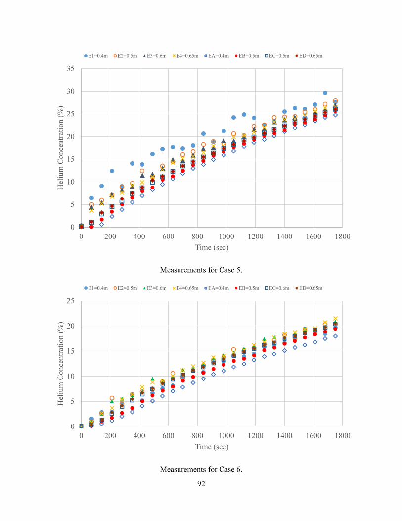
92
Measurements for Case 5.
Measurements for Case 6.
0
5
10
15
20
25
30
35
0 200 400 600 800 1000 1200 1400 1600 1800
Hel
ium
Conce
ntr
atio
n (
%)
Time (sec)
E1=0.4m E2=0.5m E3=0.6m E4=0.65m EA=0.4m EB=0.5m EC=0.6m ED=0.65m
0
5
10
15
20
25
0 200 400 600 800 1000 1200 1400 1600 1800
Hel
ium
Conce
ntr
atio
n (
%)
Time (sec)
E1=0.4m E2=0.5m E3=0.6m E4=0.65m EA=0.4m EB=0.5m EC=0.6m ED=0.65m

93
Measurements for Case 7.
Measurements for Case 8.
0
2
4
6
8
10
0 50 100 150 200 250 300
Hel
ium
Conce
ntr
atio
n (
%)
Time (sec)
E1=0.4m E2=0.5m E3=0.6m E4=0.65m EA=0.4m EB=0.5m EC=0.6m ED=0.65m
0
2
4
6
8
10
12
14
16
18
0 100 200 300 400 500 600 700 800 900
Hel
ium
Con
centr
atio
n (
%)
Time (sec)
E1=0.4m E2=0.5m E3=0.6m E4=0.65m EA=0.4m EB=0.5m EC=0.6m ED=0.65m

94
Measurements for Case 9.
Measurements for Case 10
0
5
10
15
20
25
0 200 400 600 800 1000 1200 1400 1600 1800
Hel
ium
Conce
ntr
atio
n (
%)
Time (sec)
E1=0.4m E2=0.5m E3=0.6m E4=0.65m EA=0.4m EB=0.5m EC=0.6m ED=0.65m
0
5
10
15
20
25
30
0 300 600 900 1200 1500 1800 2100 2400 2700
Hel
ium
Conce
ntr
atio
n (
%)
Time (sec)
E1=0.4m E2=0.5m E3=0.6m E4=0.65m EA=0.4m EB=0.5m EC=0.6m ED=0.65m
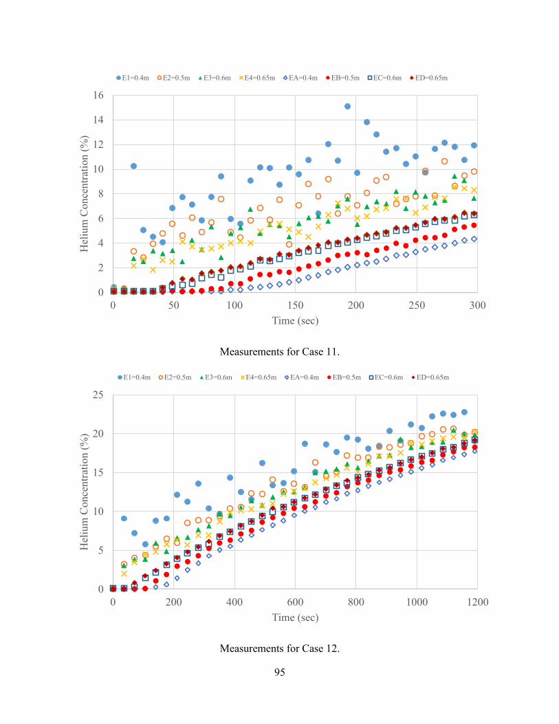
95
Measurements for Case 11.
Measurements for Case 12.
0
2
4
6
8
10
12
14
16
0 50 100 150 200 250 300
Hel
ium
Conce
ntr
atio
n (
%)
Time (sec)
E1=0.4m E2=0.5m E3=0.6m E4=0.65m EA=0.4m EB=0.5m EC=0.6m ED=0.65m
0
5
10
15
20
25
0 200 400 600 800 1000 1200
Hel
ium
Conce
ntr
atio
n (
%)
Time (sec)
E1=0.4m E2=0.5m E3=0.6m E4=0.65m EA=0.4m EB=0.5m EC=0.6m ED=0.65m
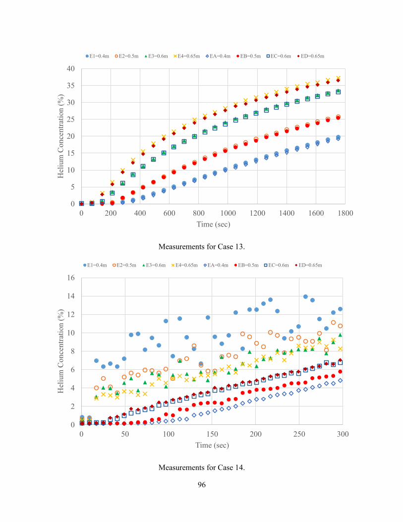
96
Measurements for Case 13.
Measurements for Case 14.
0
5
10
15
20
25
30
35
40
0 200 400 600 800 1000 1200 1400 1600 1800
Hel
ium
Conce
ntr
atio
n (
%)
Time (sec)
E1=0.4m E2=0.5m E3=0.6m E4=0.65m EA=0.4m EB=0.5m EC=0.6m ED=0.65m
0
2
4
6
8
10
12
14
16
0 50 100 150 200 250 300
Hel
ium
Conce
ntr
atio
n (
%)
Time (sec)
E1=0.4m E2=0.5m E3=0.6m E4=0.65m EA=0.4m EB=0.5m EC=0.6m ED=0.65m
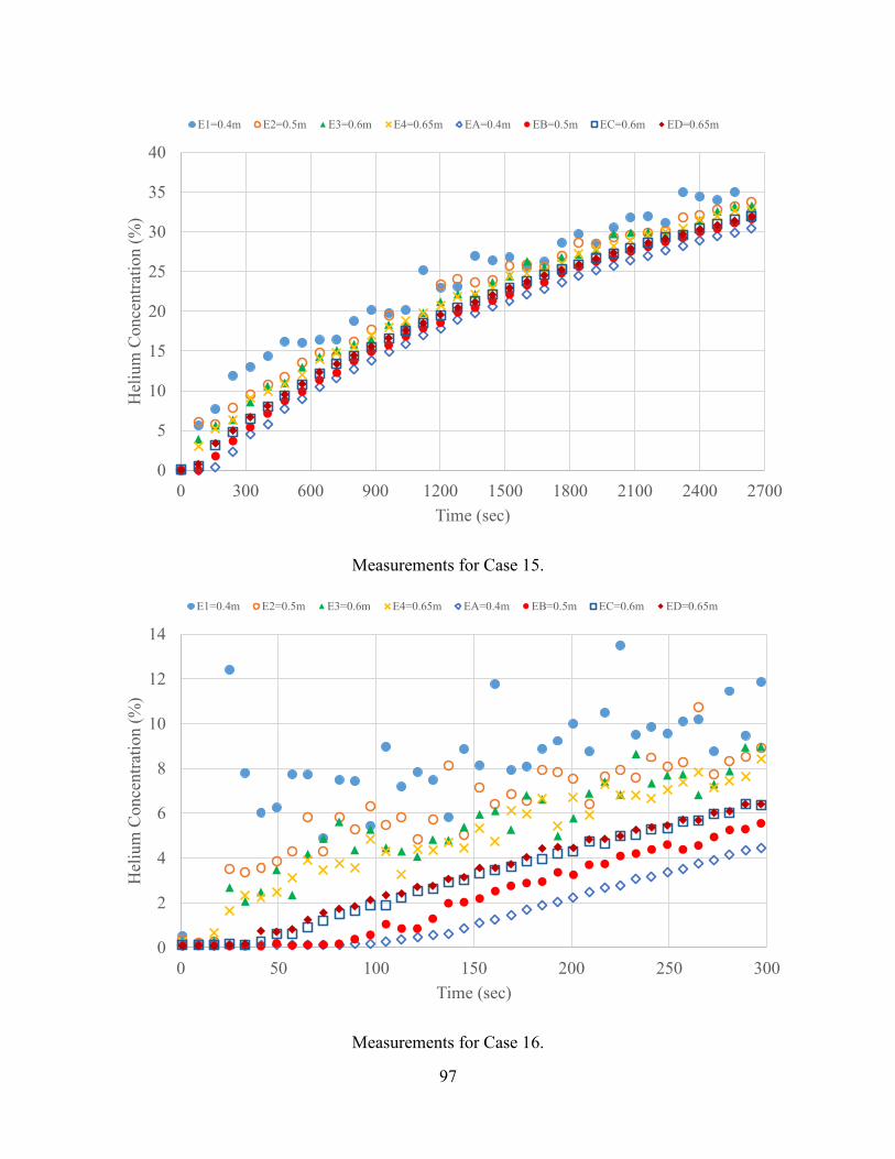
97
Measurements for Case 15.
Measurements for Case 16.
0
5
10
15
20
25
30
35
40
0 300 600 900 1200 1500 1800 2100 2400 2700
Hel
ium
Conce
ntr
atio
n (
%)
Time (sec)
E1=0.4m E2=0.5m E3=0.6m E4=0.65m EA=0.4m EB=0.5m EC=0.6m ED=0.65m
0
2
4
6
8
10
12
14
0 50 100 150 200 250 300
Hel
ium
Conce
ntr
atio
n (
%)
Time (sec)
E1=0.4m E2=0.5m E3=0.6m E4=0.65m EA=0.4m EB=0.5m EC=0.6m ED=0.65m

98
Measurements for Case 17.
Measurements for Case 18.
0
5
10
15
20
25
30
35
40
0 300 600 900 1200 1500 1800 2100 2400 2700
Hel
ium
Conce
ntr
atio
n (
%)
Time (sec)
E1=0.4m E2=0.5m E3=0.6m E4=0.65m EA=0.4m EB=0.5m EC=0.6m ED=0.65m
0
2
4
6
8
10
12
14
16
0 50 100 150 200 250 300
Hel
ium
Conce
ntr
atio
n (
%)
Time (sec)
E1=0.4m E2=0.5m E3=0.6m E4=0.65m EA=0.4m EB=0.5m EC=0.6m ED=0.65m

99
Measurements for Case 19.
Measurements for Case 20.
0
5
10
15
20
25
30
35
0 300 600 900 1200 1500 1800 2100 2400 2700
Hel
ium
Conce
trat
ion (
%)
Time (sec)
E1=0.4m E2=0.5m E3=0.6m E4=0.65m EA=0.4m EB=0.5m EC=0.6m ED=0.65m
0
5
10
15
20
25
0 200 400 600 800 1000 1200
Hel
ium
Conce
ntr
atio
n (
%)
Time (sec)
E1=0.4m E2=0.5m E3=0.6m E4=0.65m EA=0.4m EB=0.5m EC=0.6m ED=0.65m
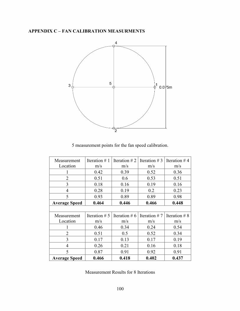
100
APPENDIX C – FAN CALIBRATION MEASURMENTS
5 measurement points for the fan speed calibration.
Measurement
Location
Iteration # 1
m/s
Iteration # 2
m/s
Iteration # 3
m/s
Iteration # 4
m/s
1 0.42 0.39 0.52 0.36
2 0.51 0.6 0.53 0.51
3 0.18 0.16 0.19 0.16
4 0.28 0.19 0.2 0.23
5 0.93 0.89 0.89 0.98
Average Speed 0.464 0.446 0.466 0.448
Measurement
Location
Iteration # 5
m/s
Iteration # 6
m/s
Iteration # 7
m/s
Iteration # 8
m/s
1 0.46 0.34 0.24 0.54
2 0.51 0.5 0.52 0.34
3 0.17 0.13 0.17 0.19
4 0.26 0.21 0.16 0.18
5 0.87 0.91 0.92 0.91
Average Speed 0.466 0.418 0.402 0.437
Measurement Results for 8 Iterations