Using geometric algebra to represent curvature in

shell theory with applications to Starling resistors

Alastair L Gregory1,*, Anurag Agarwal1, and Joan Lasenby1

1Department of Engineering, University of Cambridge,Trumpington Street, Cambridge, CB2 1PZ

*alg57@cam.ac.uk

31 October 2017

Abstract

We present a novel application of rotors in geometric algebra to repre-sent the change of curvature tensor, that is used in shell theory as part ofthe constitutive law. We introduce a new decomposition of the change ofcurvature tensor, which has explicit terms for changes of curvature due toinitial curvature combined with strain, and changes in rotation over thesurface. We use this decomposition to perform a scaling analysis of therelative importance of bending and stretching in flexible tubes undergo-ing self excited oscillations. These oscillations have relevance to the lung,in which it is believed that they are responsible for wheezing. The newanalysis is necessitated by the fact that the working fluid is air, comparedto water in most previous work. We use stereographic imaging to empiri-cally measure the relative importance of bending and stretching energy inobserved self excited oscillations. This enables us to validate our scalinganalysis. We show that bending energy is dominated by stretching energy,and the scaling analysis makes clear that this will remain true for tubesin the airways of the lung.

1 Introduction

Self excited oscillations of flexible tubes driven by fluid flow have been a sub-ject of interest for some time, and there is a considerable literature on thesubject, which is reviewed by [1–6]. Experimental rigs designed to study thisphenomenon are often called Starling resistors. We are interested in this phe-nomenon because of its possible relevance to wheezing in the lung [7], which isone of the most commonly heard lung sounds used for diagnosis [8, 9]. Previouswork on Starling resistors has largely used water as the working fluid. In thelung the working fluid is air. This means that the density ratio between theworking fluid and the tube material in the lung is significantly different from

1

arX

iv:1

710.

1154

2v1

[m

ath-

ph]

31

Oct

201

7

almost all of previously completed work on Starling resistors. Previous mod-elling work usually neglects wall inertia, using instead a “tube law” [10], butthere is strong evidence that wall inertia is significant in the lung from [8, 11],who showed that when the density of the fluid breathed in is changed, the fre-quency of the wheezes is not affected significantly. It is clear therefore that thechange in density ratio results in a qualitatively different mechanism. For thisreason we have been conducting our own experiments, and creating models tounderstand the onset of oscillations.

The flexible tube itself is generally modelled as an elastic shell. Traditionalshell theories [12–17] are well developed but difficult to implement. We havefound that linearised shell theories do not provide good predictions of the fre-quencies of oscillation, and we believe that this is due in part to the fact thatwe have observed that oscillations start from a collapsed or partially collapsedstate. To use current geometrically non-linear shell theories would require a nu-merical simulation of a very complex fluid structure interaction problem, whichwould be of similar value to experimental results (though arguably harder toimplement), and would provide the same problem of being difficult to physi-cally interpret due to the complex nature of the oscillations observed. Insteadwe would like to gain a physical understanding of the important mechanismsbehind the oscillations, and this is difficult with shell theories based in differen-tial geometry [14, 15], in particular due to the lack of physical interpretationsof the change of curvature tensor in general situations. We recently introducedgeometric algebra to shell theory [18], which allowed us to express the funda-mental laws in a component-free form and clarify the role of angular velocityand moments through the use of bivector representation. For an introductionto the basics of geometric algebra see [19]. One of the most powerful aspects ofgeometric algebra lies in the use of rotors to represent rotations. In [20] thesehave been used to simplify Simo and Vu Quoc’s numerical algorithm [21] formodelling the nonlinear behaviour of rods. In projective and conformal geom-etry [19, §10] rotors have allowed geometric primitives to be represented in amore simple and lucid manner, and in relativity [22] and relativistic analogies[23] rotors can simplify transformation between frames of reference. In thispaper we make use of rotors to better understand the change of curvature ofa shell, which is of prime importance to the constitutive law of the shell, butwhose representation has long caused controversy. In [12] at least 10 differentlinearised shell theories are presented, and the differences are primarily causedby disagreements over how to represent changes of curvature. [14] has provideda tensor definition of the change of curvature that has become accepted, how-ever, the utility of this expression is limited by its complexity. We have beenable to simplify the representation of this tensor using rotors, allowing a morelucid and physical interpretation of changes of curvature. We take advantage ofthis to allow us to understand the importance of the change of curvature in thecontext of our Starling resistor experiments.

In order to compare results from the shell theory to our experimental resultswe need to be able to calculate the kinematic parameters associated with thedeformation of the flexible tube. To enable this we use stereoscopic imaging,

2

which to our knowledge is the first time it has been used in the study of Starlingresistors. We take high speed video of the tube at the onset of oscillation,and are able to track the motion of the surface, and consequently compare thepredictions of shell theory with empirical calculation.

2 Understanding Changes in Curvature

There is an energy associated with any deformation of a shell, and Koiter [17]proposes the following form for this energy,

ρ0U =Eh

2(1− ν2)

((1− ν) tr(E2) + ν tr(E)2

)+

Eh3

24(1− ν2)

((1− ν) tr(H2) + ν tr(H)2

).

(1)U is the internal energy per unit mass of the shell, defined on the reference con-figuration, ρ0 is the time independent area density of the shell on the referenceconfiguration, E is Young’s modulus, ν is Poisson’s ratio, h is the shell thick-ness (which in Koiter’s theory is assumed constant), E is the two-dimensionalGreen-Lagrange strain tensor defined on the reference configuration, H is thechange of curvature tensor, and tr is the trace operator. From (1) we can derivethe governing equations of the shell (for more details see [18]). The first termon the right hand side of (1) represents the stretching energy, and the secondterm represents the bending energy.

In general a shell is a body in which the thickness is smaller than the otherrelevant defining length scales. The use of (1) for the energy of deformationimplies that we additionally assume that the midsurface of the body remains themidsurface under deformation, a material line that is normal to the midsurfaceremains normal to it under deformation, the shell thickness remains constantwith time, the first and second moments of density relative to the midsurfaceare zero, strains within the shell are small, and so is the normal stress (see [18]for further discussion).

Following the notation of [18] we take B and S to be the reference andspatial configurations of the shell, and X ∈ B and x ∈ S to be locations onthese configurations. φt is the motion of the shell, meaning that at time t, thepoint X ∈ B is at the position φt(X) ∈ S. G and g are the identity functionson the reference and spatial configurations. Y and y are vectors within thetangent spaces of B and S respectively. {Xi}, i = 1, 2 is a coordinate systemon the reference configuration B, which we can then use to define the frame onthe reference configuration {Ei = ∂X/∂Xi}. {Ei} is the reciprocal frame thatsatisfies Ei · Ej = δij . {xi}, {ei} and {ei} are the similarly defined coordinatesystem, frame, and reciprocal frame on the spatial configuration. The shellundergoing deformation is embedded within a flat three-dimensional Euclideanspace E3.

If A and B are general multivectors, then AB is the geometric productbetween them, A ·B is the inner product, A∧B is the outer product, and A×Bis the commutator product, defined by A×B = 1

2 (AB −BA) (see [19, §4.1.3]).

3

We also take ××× (compared to ×) to be the cross product between two vectors.If I is the pseudoscalar of a three-dimensional space, and a and b are vectors,then a××× b = −Ia ∧ b.

We are particularly interested in the change of curvature that is encoded in H.To understand this we must understand the curvature tensors on the referenceand spatial configurations B and b. If E3 and e3 are the normal vectors to thereference and spatial configurations respectively, then B(Y ) and b(y) are givenby,

B(Y ) = −Y · ∂E3, b(y) = −y · ∂e3, (2)

where ∂ is the intrinsic vector derivative to any surface. The relationship be-tween ∂ and the vector derivative of E3 is explained in [18]. On B we can expand∂ as ∂ = Ei∂/∂Xi and on S we can expand it as ∂ = ei∂/∂xi [19, §6.5.1]. Band b give non-zero results if the surface is not flat. The change of curvaturetensor H is given by,

H(Y ) = FbF(Y )− B(Y ), (3)

where F is the deformation gradient, defined by F(Y ) = Y ·∂φt(X). F maps fromthe tangent space of B to the tangent space of S, providing information aboutthe local deformation of the surface. F is the adjoint of F, i.e. F(Y ) ·y = Y · F(y).The strain tensor E, used in the constitutive law (1), is given by,

E(Y ) =1

2

(FF(Y )− Y

). (4)

This much is well known, though in other treatments coordinate dependentdefinitions of H are used (e.g. in [14]). To make further progress we will nowuse rotors to better understand what will produce changes in H.

To begin, we note that we can perform a polar decomposition on F suchthat F(Y ) = RU(Y ) where R = R−1, detR = 1, and U = U. R encodes rotation,and U encodes stretching. We can choose to consider a frame {Ei} on thereference configuration that is locally orthonormal1. In this case E3 = E1×××E2 =−I3(E1 ∧ E2) = −I3(E1E2), where I3 is the pseudoscalar of three-dimensionalEuclidean space E3.

To find e3 we need two unit vectors in the tangent space of the spatialconfiguration that are oriented in the same way as the pair F(E1),F(E2), andare orthonormal. This pair of unit vectors is given by R(E1),R(E2), and so e3 isgiven by e3 = R(E1)××× R(E2) = −I3(R(E1) ∧ R(E2)) = −I3(R(E1)R(E2)). Thefact that the function R is a rotation means that it has an associated rotor R suchthat R(Y ) = RYR, where R is an even multivector that satisfies RR = RR = 1,where R is the reverse of R. This allows us to write e3 as,

e3 = −I3(

(RE1R)(RE2R))

= −I3(R(E1E2)R

)= RE3R, (5)

where we have used the fact that any rotor will commute with I3. Thus we haveshown that the rotation associated with the deformation is also the rotation

1The coordinate system {Xi} must be chosen such that this is the case, and it may benecessary to use several overlapping coordinate systems to achieve this.

4

between the normal vectors E3 and e3, which makes intuitive sense. We havealso extended the range and domain of R to E3, while the range and domainof U is still constrained to the tangent space of the reference configuration, andthe range and domain of F are constrained to the tangent spaces of the spatialand reference configuration respectively.

Two results that we will find useful are,

Y · ∂R = −R(Y · ∂R)R, (6a)

F(Y ) · ∂e3 = Y · ∂e3. (6b)

(6a) follows from RR = 1. (6b) has implicit assumptions that require explana-tion. The expression on the left of (6b) tells us how e3 varies over the spatialconfiguration in the direction defined by F(Y ), which lies in the tangent space ofthe spatial configuration. On the right of (6b), e3 = e3(x) has been mapped to avector field on the reference configuration such that e3(X) = e3(φt(X)) ∀X ∈ B.This allows the expression on the right to tell us how e3 varies over the referenceconfiguration in the direction defined by Y , which is tangent to the reference con-figuration. The equality of these expressions is a standard result when mappingderivatives between manifolds, which can be proven by considering derivativeswith respect to convected coordinates that satisfy xi(x) = Xi(φ−1

t (x)). Fromthis point we will assume that {xi} are convected coordinates.

Using these results we can write FbF(Y ) as FbF(Y ) = −F(Y · ∂e3), and theargument of F can be expressed as,

Y · ∂e3 = Y · ∂(RE3R) = (Y · ∂R)E3R+R(Y · ∂E3)R+RE3(−R(Y · ∂R)R)

= R(Y · ∂E3)R+ [(Y · ∂R)R]RE3R−RE3R[(Y · ∂R)R]

= R(Y · ∂E3)R+ [(Y · ∂R)R]e3 − e3[(Y · ∂R)R]

= R(Y · ∂E3)R+ [2(Y · ∂R)R]× e3= R(Y · ∂E3) + [2(Y · ∂R)R]× e3,

(7)where × is the commutator product. Hence we can express FbF(Y ) as,

FbF(Y ) = −FR(Y · ∂E3)− F(

[2(Y · ∂R)R]× e3)

= −U(Y · ∂E3)− F(

[2(Y · ∂R)R]× e3)

= UB(Y ) + F(e3 × [2(Y · ∂R)R]

),

(8)

and finally we obtain an expression for H,

H(Y ) = (U− G)B(Y ) + F(e3 × [2(Y · ∂R)R]

)= (U− G)B(Y ) + F

([RE3R]× [2(Y · ∂R)R]

).

(9)

This shows that there are two contributions to H. Firstly, if the referenceconfiguration is at all curved (i.e. B(Y ) is non-zero), then the strain of the shell,

5

encoded in U−G, will result in a change of curvature. The second contributionis due to variation of the rotor R over the shell. These two kinds of change ofcurvature are illustrated well by an inflating sphere and deformation of a flatplate. As a sphere is inflated to become a larger sphere, the normal vector isunchanged, i.e. e3 = E3, hence R = 1 everywhere. This means that the secondterm in our expression for H will be zero. However, the surface of the sphere willstretch, meaning that U − G will be non-zero. In addition, B will be non-zerofor a sphere, which tells us that the first term in our expression for H will benon-zero. By contrast, for a flat plate B(Y ) will be zero, meaning that R mustvary over the plate in order for there to be any change of curvature.

A variant on this expression for H can be obtained if we express the rotor Ras R = exp(−A/2) = exp(−Aθ/2), where A is a bivector aligned with the planeof rotation whose magnitude is equal to the angle of rotation θ. A is a unitbivector (A2 = −1). Note that the direction of rotation is defined by the signof θ and the orientation of A together. We can set the convention that θ > 0,in which case θ and A are uniquely defined if A is known. Given this definitionwe can express Y · ∂R as,

Y · ∂R = −Y · ∂A2

exp(−A/2) = −Y · ∂A2

R. (10)

Using this we can express H as,

H(Y ) = (U− G)B(Y )− F(

(RE3R)× (Y · ∂A)). (11)

The term that F operates on is the commutator product of a vector and bivector,so we can replace the commutator product with a dot product,

H(Y ) = (U− G)B(Y )− F(

(RE3R) · (Y · ∂A)). (12)

Taking the inner product of a bivector with RE3R = e3 means that only vectorstangential to the spatial configuration are retained, which then means that Fcan operate and return vectors tangential to the reference configuration. Henceour description confirms that the range and domain of H are both the tangentspace of the reference configuration.

The explicit expression for the two possible contributions to change of curva-ture, shown in (12), gives a new decomposition of the change of curvature tensorwhich will be of use when we try to understand the importance of bending inthe Starling resistor.

3 Experiment Description

3.1 Experimental Setup

Figure 1 shows a schematic of the experimental setup used to investigate the os-cillations of flexible tubes. Air flows into the system through (1), then through

6

1

82

3

45 6 7 6’ 5’

3’

Figure 1: Schematic of Starling resistor experiment. 1: Flow inlet, 2: Ro-tameter, 3/3’: Settling chambers, 4: Clean flow inlet, 5/5’: Clean flow tubes,6/6’: Contraction and expansion, 7: flexible tube, 8: tube to suction fan. Thedownstream settling chamber is approximately 4 m3 while the upstream settlingchamber is 0.03 m3.

a rotameter (2) used to monitor flowrate. The noise that the rotameter intro-duces into the flow, and any other noise, is isolated from the flexible tube by theupstream settling chamber (3). Air flows into the upstream clean flow tube (5)section via a shaped inlet (4) that reduces separation. A contraction (6) leadsto the flexible tube (7), before an expansion (6’) leads to the downstream cleanflow tube (5’) that exits into the downstream settling chamber (3’). Suctionis provided by a fan (8). The downstream settling chamber (3’) isolates theflexible tube from the noise from this fan. Experiments were performed in theAcoustics Laboratory in the Department of Engineering at the University ofCambridge.

In the experiments relevant to this paper the suction at (8) is graduallyincreased until the flexible tube just starts oscillating. With the tube oscillatingin this way high speed video is recorded from 2 FASTCAM-ultima APX cameras(produced by Photron https://photron.com) with a frame rate of 12 500 fpsand a resolution of 512× 256 pixels (grayscale). Our experiments require us tofocus on a small flexible tube at reasonably close range. The Photron camerahas an adaptor for Nikon lens’s. We use a 50 mm lens combined with a 7 mmextension tube to allow us to focus on the tube and have it fill most of the frame.An aperture of f/2.8 is used.

The flexible tubes used are made out of rubber latex for which E = 1 MPaand ν = 0.5. The tube diameter is 6 mm, the wall thickness is 0.3 mm and theunstrained length is 19 mm. The tubes are held in an axially strained state, sothe length of the tubes during the experiment is 25 mm.

3.2 Image Processing

The high speed cameras record at 12 500 fps, and are triggered together, so thatevery ∆t = 80 µs two images of the flexible tube are taken. A schematic of thetwo cameras and the flexible tube is shown in Figure 2. Dots are drawn on

7

flexible tube

camera 1 camera 2

focal point of camera 1 focal point of camera 2

dots drawn on flexible tube

dots seen inboth cameraplanes

dot of interest,dot i (of n)

dot i seen incamera 1

dot i seen incamera 2

Figure 2: Schematic of the high speed camera setup.

the flexible tube (shown in white in Figure 2), which indicate a set of materialpoints we would like to track over time in three dimensions.

It is possible to find the characteristics2 of two cameras such that if a pointappears in simultaneous images from both cameras, the point’s position in three-dimensional space can be triangulated [24, 25]. Calibration involves taking atleast 3, and in general between 10 and 20, simultaneous images of a chequer-board pattern in various orientations. From this the position of the two cam-eras relative to each other, and their internal parameters, can be calculated. Inthis method cameras are modelled as pinhole cameras, meaning that the focallength, pixel size and skew are the important internal parameters. In addition itis possible to account for radial distortion of the image by the camera lens, andtangential distortion, which occurs when the image sensor is not perfectly per-pendicular to the line of sight of the camera. This calibration is performed usingthe computer vision system toolbox of Matlab R© [26]. The images producedby these pinhole camera models is what is illustrated in Figure 2.

To find the three-dimensional tracks of the material points, we must firstfind the locations of the dots within each image. We refer to these coordinatepairs as points. The dots on the tube surface are drawn in white, are spaced byapproximately 1 mm, and have a diameter of approximately 0.7 mm. We takethe material points to be the centres of the dots, and we find them by first takinga two-dimensional convolution of the image with a “mexican hat” function of

2The characteristics of an imaginary pinhole camera that we replace the real camera withto allow us to use methods from projective geometry to perform the triangulation.

8

the form,

1

πσ4

(1− x2 + y2

2σ2

)e−

x2+y2

2σ2 , (13)

where σ is the expected radius of the dot in the image. The convolution effec-tively smooths the image, removing any artefacts from drawing the dots, leavingpeaks in the centroid of each dot. These peaks are then used as the locations ofeach point.

Hence at each time instance, we have two collections of points, representingthe material points as seen from each camera. If there are n points on the tube,and m frames in our video, then in total we will have found the locations of2nm points. To make use of this data, we need to identify each unique materialpoint in each camera and over time.

To associate points across time for a single camera’s set of images, the pointsat t and t + ∆t are compared, and if two points are within a certain distanceof each other, then it is assumed that these represent the same point. Thisworks because the frame rate (12 500 fps) is much larger than the frequency ofthe observed vibrations (∼ 500 Hz), so motions between frames are small.

A pair of corresponding points in the two camera images are illustrated inFigure 2, but finding these pairings at each instant in time is more complex.First we consider the line drawn from the focal point of camera 2 to dot i inthe image, which we will call a ray. Anything on this ray in three-dimensionalspace will appear at the same highlighted location in camera 2. However, fromcamera 1, the ray will appear as a line. Therefore, if a point’s location is knownin one camera image, then it must lie on a specific line in the other image.This line is known as an epipolar line [25]. Hence, for a pair of points, onein each camera image, to correspond to the same material point, they musteach lie on the epipolar line of the other. However, because of the specificarrangement of the cameras and dots, this does not usually provide a uniqueset of pairs. The relative positioning of the cameras means that the epipolarlines are all approximately horizontal, and the dots drawn on the tube arearranged in horizontal rows, so multiple dots can be very close to a given epipolarline. To overcome this, we specify 10 corresponding point pairs between thetwo images (20 points in total), and these 10 pairs are then used to find thebest fitting projective transformation from camera 1 to camera 2. Applyingthis transformation to the image from camera 1 places each point close to thecorresponding point in the image from camera 2, allowing all the remainingpoint pairs to be found. This result is then checked for consistency with theepipolar line condition.

In addition to tracing material points over time as the self excited oscillationsoccur, we must also find the locations of the material points on the tube whenit is unstrained. This is necessary for the calculation of the kinematic variablesused in expression for energy of deformation (1). To achieve this a single imageis taken from each camera when the tube is held in its unstrained state. Pairingof points must then also be completed between the two images of the tube in itsunstrained state and images from the high speed video of self excited oscillations.

9

This pairing is done using the methods described in the previous paragraph.Once point pairs are known over time, the camera calibration can be used

to find three-dimensional point traces over time. The spatial resolution of thistrace is limited by the size of the pixels in the high speed video. This results inpoint traces with distinct jumps in position. These jumps are by no more than0.1 mm in three-dimensional space, compared to variations in position on theorder of 2 mm over the course of the self excited oscillations. For this reason wesmooth the three-dimensional point traces by fitting functions of the form,

8∑i=1

Ai sin(ωit), (14)

to the three position components, where Ai and ωi are chosen to fit the empiricaldata. These fits work well because the videos are of quasi-steady behaviour atthe onset of oscillation, and the observed motions are close to sinusoidal. 8 termshave been found to be sufficient to match the experimental data. This smoothingis necessary in order for derivatives of the point traces to give meaningful results.

3.3 Kinematic Calculations

In Figure 3 we show a single frame from the video in which the dots on thesurface of the tube have been automatically detected, identified with the corre-sponding dots in the other video image, and identified with the correspondingdots in a stereoscopic image of the unstrained tube (not shown). With thisinformation we can reconstruct the points in three dimensions and fit a surfaceto them. The process can be summarised as follows,

• Locate points in images of unstrained tube.

• Track points in high speed video frames.

• Associate points between all images (as described in §3.2) and triangulateto have the position of each material point as a function of time, and itsposition on the unstrained tube.

• Assign a pair of coordinate values {xi} to each point for use as the con-vected surface coordinates.

• Fit a smoothing curve to every three-dimensional point as a function oftime as described in §3.2.

• At a chosen time take the positions of all of the points and fit a polynomialsurface such that we have position as a function of the surface coordinates{xi}. Repeat this for the unstrained surface.

• Take all possible first and second derivatives of the surface position withrespect to {xi}. This is done analytically using the polynomial surface.Repeat this for the unstrained surface.

10

Figure 3: A typical image of the principal strains of the flexible tubes, shownalong with the principal strain directions (illustrated with unit vectors). On theleft the original high speed camera images are shown with the tracked surfacepoints, and a view of the three-dimensional triangulation with the surface fittedto them.

The surface fit and its derivatives are used to calculate all the kinematic prop-erties of the undeformed and deformed surfaces.

In Figure 3 we show a typical image of the principal strains of the flexibletube, i.e. the eigenvectors and values of E. An eigenvalue of 1 corresponds to nostrain, a value less than 1 corresponds to compression, and a value greater than1 corresponds to tension. The eigenvectors give the direction in which the strainis occurring. We can see that the first principal strain is approximately alignedwith the longitudinal direction, and is tensile. This is due to the dominantpre-strain of the elastic tube. By contrast, the second principal strain, which isprimarily in the azimuthal direction, is a mixture of compression and tension,and is generally closer to 1. In Figure 4 we show the principal curvatures ofthe deformed surface, i.e. the eigenvectors and values of b. For a cylinder,which the tube is in its undeformed state, the principal curvatures would be 0in the longitudinal direction and 1/a = 0.33 mm−1 in the azimuthal direction.We see that in the deformed tube the curvatures are still closely aligned to thelongitudinal and azimuthal directions, and can see that the squashing of thetube results in a slightly negative longitudinal curvature and a slight reductionin the azimuthal curvature towards the centre of the tube. But these effects arefairly small.

11

Figure 4: A typical image of the principal curvatures of the flexible tube, shownalong with the principal curvature directions (illustrated with unit vectors).

12

4 Calculation of Bending and Stretching Ener-gies

We now aim to gain more understanding of how the tube deforms. To do this wewill use a mixture of empirical and analytical techniques. More specifically wecan use the high speed video reconstructions combined with the mathematicalframework for shells already developed in §2.

4.1 Scaling Analysis

We start by estimating the bending and stretching energies analytically, whichrequires us to estimate the values of tr(E2), tr(E)2, tr(H2), and tr(H)2.

If αi are the eigenvalues of the linear function A, then tr(A)2 = α21 +2α1α2+

α22 and tr(A2) = α2

1+α22. We know that the eigenvalues of E are 1

2 (λ2i−1) (λi arethe principal strains) and that λ1 ∼ λ, λ2 ∼ 1, where λ is the initial axial strainof the tube. This allows us to get an order of magnitude estimate for tr(E2) andtr(E)2 of (λ2 − 1)2/4. If we take λ = 1.33 then we have tr(E2) ∼ tr(E)2 ∼ 0.1.

To understand bending in the tube we consider the representation of Hderived in §2, and given in (12). We can write the action of U(Y ) as U(Y ) =λ1(Y · W1)W1 + λ2(Y · W2)W2, where Wi are the unit eigenvectors of U. Usingthe approximation λ1 ≈ λ and λ2 ≈ 1 this becomes U(Y ) ≈ λ(Y · W1)W1 +(Y · W2)W2. We can write B(Y ) as B(Y ) = C(Y · E2)E2, where Ei are the uniteigenvectors of B, and C is the principal curvature of the undeformed tube inthe azimuthal direction. Combining these we have,

UB(Y )− B(Y ) = U(CY · E2E2)− CY · E2E2

≈ CY · E2(λE2 · W1W1 + E2 · W2W2)− CY · E2E2.(15)

We know from Figure 3 that W1 and W2 are approximately aligned with thelongitudinal and circumferential directions, so we can write E2 · W1 ≈ 0 andE2 · W2 ≈ 1. Using this we obtain,

UB(Y )− B(Y ) ≈ CY · E2W2 − CY · E2E2 ≈ 0. (16)

This is saying that because the directions of principal strain and principal cur-vature are approximately perpendicular, the influence of strain on change ofcurvature is removed.

We are now in a position to consider the rotor R, since it is changes in thismultivector over the surface of the shell that are responsible for the change ofcurvature. R represents the rotation, and as is shown in §2 is characterised bythe bivector A = θA, whose magnitude gives the rotation angle in radians, andwhose plane gives the plane of rotation. In Figure 5 we visualise the angle andaxis of rotation encoded in the rotation tensor R, corresponding to a typicaldeformation. The axes of rotation shown in Figure 5 are primarily tangential to

3The strained length of the tube is l = 25 mm and the unstrained length is l0 = 19 mm,giving λ = l/l0 ≈ 1.3.

13

Figure 5: A visualisation of the rotation R. The axis of rotation is shown alongwith the absolute value of the angle of rotation (in radians).

the surface, so the bivector A will be dominated by the components e1 ∧ e3 ande2 ∧ e3, with little rotation in the e1 ∧ e2 plane, i.e. about the normal vector e3.Hence, we can write A as,

A = θ1e1 ∧ e3 + θ2e

2 ∧ e3 = θiei ∧ e3. (17)

We have used the reciprocal frame {ei} instead of of {ei} because it will allow usto use the property F(ei) = Ei4. We can extend the frames {ei} and {ei} to spanE3 by using the normal vector e3. Because e3 is a unit vector and perpendicularto all of ei, e

i, we can also write e3 = e3, and we have the frame {ea}, a = 1, 2, 3and {ea}. Using this we define the Christoffel coefficients γaib = ea · ∂eb/∂xi,i = 1, 2; a, b = 1, 2, 3. These also satisfy eb · ∂ea/∂xi = −γaib.

Substituting A into the second part of the change of curvature tensor givenin (12), using the fact that e3 is normal to e1 and e2, and γ3i3 = 0, we obtain,

F(e3 · (Y · ∂A)

)= Y iF

(−∂i(θj)ej + θjγ

jike

k)

= −Y i∂i(θj)Ej + Y iθjγ

jikE

k.(18)

Therefore, given that the first part of H in (12) is zero, Ei ·H(Ej) = Hij is givenby,

Hij = ∂jθi − θkγkji. (19)

We know that H is symmetric, so from this we see that our earlier assumption onthe form of A must be joined by the condition ∂iθj = ∂jθi to produce consistentresults.

The frame {Ei} can be chosen by us to be orthonormal. More specifically,we can align E1 with the longitudinal direction and E2 with the azimuthaldirection on the unstrained cylindrical tube. From Figure 3 we can see that

4The coordinate system is convected, so ei = F(Ei), and as always ei · ej = Ei · Ej = δij .

Hence δij = ei · F(Ej) = F(ei) · Ej , from which it is clear that F(ei) = Ei.

14

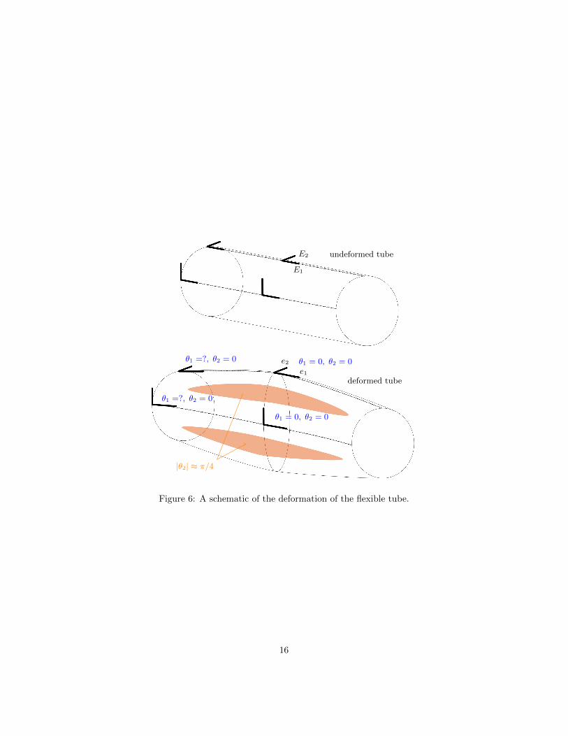
under a typical deformation these basis vectors remain close to the axial andazimuthal directions. In Figure 6 we give a schematic illustration of how Ei

maps to ei. In Figure 6 we have also labelled the values of θi where they areobvious. The regions where |θ2| ≈ π/4 can be seen empirically in Figure 5.There are two unknown values of θ1 shown as question marks. We can estimatethe largest value of these rotations by assuming a straight line from the clampedtube end and the centre of the tube when the tube collapses completely at thecentre. In this case θ1 ∼ arctan(a/(l/2))λ where a is the tube radius and l is thetube length in its deformed state. The multiplication by λ is necessary becauseθ1 is the e1 ∧ e3 component, and e1 is shortened by a factor of λ compared tothe unit vector E1. Up to angles of 30◦, tan θ is within 10 % of θ, so we will takeθ1 ∼ λa/(l/2) = a/(l0/2) at the point in question, where l0 is the unstrainedlength of the tube. This, and the values of θi shown in Figure 6, allows us tomake the following estimates,

∂1θ1 ∼a

l0/2

1

l0/2=

4a

l20,

∂1θ2 = ∂2θ1 ∼π/4

l0/2=

π

2l0,

∂2θ2 ∼π/4

2πa/8=

1

a.

(20)

Because of replacement of arctan with the identity function, our estimate for∂1θ1 will be an overestimate when the tube is very short.

We can also estimate the values of the coefficients γijk using Figure 6,

∂1e1 ∼a

(l0/2)2e3,

∂2e1 = ∂1e2 ∼ 0,

∂2e2 ∼1

ae3.

(21)

From this we see that the changes in the basis vectors are primarily in the e3direction, meaning that they do not contribute to Hij .

If we take l0 to be much larger than a, then the dominant term in Hij willbe 1/a, but even if l0 and a are a similar order of magnitude, all of the Hij

terms will be of the order 1/a. Hence, we expect tr(H2) and tr(H)2 will scale as(1/a)2 = (1/3 mm)2 = 0.1 mm−2.

Given these scalings for tr(E2), tr(E)2, tr(H2), and tr(H)2, and the valuesE = 1 MPa, ν = 0.5, and h = 0.3 mm, we can obtain scalings for the bendingand stretching energy given in (1),

stretching energy ∼ 0.02 N mm−1,

bending energy ∼ 1.5× 10−4 N mm−1,(22)

This indicates that given the kind of deformation we have observed in our Star-ling resistors at onset, i.e. where the strain energy is dominated by the effects of

15

E1

E2

e1

e2 θ1 = 0, θ2 = 0

θ1 = 0, θ2 = 0

θ1 =?, θ2 = 0

θ1 =?, θ2 = 0

|θ2| ≈ π/4

undeformed tube

deformed tube

Figure 6: A schematic of the deformation of the flexible tube.

16

Figure 7: Values of the kinematic variables tr(E2), tr(E)2, tr(H2), and tr(H)2.

pre-strain, the axis aligned with the largest strain remains close to perpendic-ular to the axis aligned with the largest curvature, rotations are mostly aboutaxes tangential to the shell, and changes in the rotation scale with the changeof rotation about the longitudinal axis in the azimuthal direction, stretchingenergy will dominate bending energy. Moreover, this result remains valid evenwhen the tube length gets close to the tube diameter. This is significant forour considerations of the lung, since the length to diameter ratio of tubes in thelung typically varies from 1 to 6 [27].

4.2 Direct Calculation from Data

We can use the high speed video data to calculate tr(E2), tr(E)2, tr(H2), andtr(H)2 from (1). Typical plots are shown in Figure 7, from which we see that inthe units chosen these have similar orders of magnitude. We also see that thescalings obtained in the previous section agree with these plots well, providingsupport for the assumptions made. We can also calculate the bending andstretching energy, and this is shown in Figure 8. This agrees very well with thescaling values of the previous section, again supporting our conclusions.

5 Conclusions

We have developed a new method of representing the change of curvature tensorusing rotors (see (12)), increasing our understanding of bending in shells. Wehave used this representation to explain results from stereographic imaging ofStarling resistors that demonstrate that the bending energy in these deforma-

17

Figure 8: The stretching energy (top image) and bending energy (bottom image)associated with the deformation of the flexible tube.

18

tions is around 2 orders of magnitude lower than the stretching energy. We havebeen able to show that this relies on the fact that the strain energy is dominatedby the effects of pre-strain, the axis aligned with the largest strain remains closeto perpendicular to the axis aligned with the largest curvature, rotations aremostly about axes tangential to the shell, and changes in the rotation scalewith the change of rotation about the longitudinal axis in the azimuthal direc-tion. Further to this, our scaling analysis remains valid even when the tubelength gets close to the tube diameter. This is of significance to our work inunderstanding wheezing, since the length to diameter ratio of tubes in the lungtypically varies from 1 to 6. Hence we have provided a scaling analysis, con-firmed by experiment, that allows us to say that bending energy is dominatedby stretching energy during self excited oscillations in the airways of the lung.This should allow the use of membrane theory to model the tube, which reducesthe order of the equations of motion from 4 to 2.

Ethics This paper adheres to the Royal Society publishing and research ethicspolicy.

Data Accessibility Data for this paper can be accessed athttps://doi.org/10.17863/CAM.10363.

Author Contributions The work was completed as part of the PhD projectof AG, with AA supervising, and JL advising, in particular on image processingand the uses of geometric algebra.

Competing Interests The authors declare no competing interests.

Funding The authors would like to acknowledge funding from the EPSRC,the IMechE Postgraduate Research Scholarship, and Engineering for ClinicalPractice (http://divf.eng. cam.ac.uk/ecp/Main/EcpResearch).

Acknowledgements Our lab technician John Hazelwood, who has been in-strumental in the experimental work completed, and Holger Babinsky, who pro-vided advice on the use of high speed cameras.

References

[1] Heil, M. & Jensen, O. E. 2003 Flows in deformable tubes and channels.In Flow past Highly Compliant Boundaries and in Collapsible Tubes (eds.P. W. Carpenter & T. J. Pedley), pp. 15–49. Kluwer Academic Publishers.

[2] Bertram, C. D. 2003 Experimental Studies of Collapsible Tubes. In Flowpast Highly Compliant Boundaries and in Collapsible Tubes (eds. P. W.Carpenter & T. J. Pedley), pp. 51–65. Kluwer Academic Publishers.

19

[3] Grotberg, J. B. & Jensen, O. E. 2004 Biofluid Mechanics in Flexible Tubes.Annu. Rev. Fluid Mech., 36(1), 121–147.

[4] Heil, M. & Hazel, A. L. 2011 Fluid-Structure Interaction in Internal Phys-iological Flows. Annu. Rev. Fluid Mech., 43(1), 141–162.

[5] Kisilova, N., Hamadiche, M. & Gad-El-Hak, M. 2012 Mathematical modelsof biofluid flows in compliant ducts. Arch. Mech., 64(1), 65–94.

[6] Jensen, O. E. 2013 Instabilities of flows through deformable tubes andchannels. In Mechanics Down Under - Proceedings of the 22nd InternationalCongress of Theoretical and Applied Mechanics, ICTAM 2008, pp. 101–116.

[7] Grotberg, J. B. & Davis, S. H. 1980 Fluid-dynamic flapping of a collapsiblechannel: sound generation and flow limitation. J. Biomechanics, 13(3),219–230.

[8] Forgacs, P. 1978 Lung Sounds. Bailliere Tindall.

[9] Bohadana, A. B., Izbicki, G. & Kraman, S. S. 2014 Fundamentals of lungauscultation. N Engl J Med, 370(8), 744–751.

[10] Whittaker, R. J., Heil, M., Jensen, O. E. & Waters, S. L. 2010 A RationalDerivation of a Tube Law from Shell Theory. Q. J. Mech. Appl. Math.,63(4), 465–496.

[11] Shabtai-Musih, Y., Grotberg, J. B. & Gavriely, N. 1992 Spectral contentof forced expiratory wheezes during air, He, and SF6 breathing in normalhumans. J. Appl. Physiol., 72(2), 629–635.

[12] Leissa, A. W. 1973 Vibration of shells. Tech. Rep. NASA SP-288, NationalAeronautics and Space Administration, Washington D.C.

[13] Naghdi, P. M. 1972 The theory of shells and plates. In Handb. derPhys. (Encyclopedia Physics), Band (Volume) VIa/2, FestkorpermechanikII (Mechanics Solids II) (eds. S. Flugge & C. Truesdell), pp. 425–640.Springer-Verlag.

[14] Ciarlet Jr, P. G. 2005 An introduction to differential geometry with appli-cations to elasticity. J. Elast., 78-79, 1–215.

[15] Antman, S. S. 2005 Nonlinear Problems of Elasticity. Berlin: Springer-Verlag, 2nd edn.

[16] Lacarbonara, W. 2012 The Nonlinear Theory of Plates. In Nonlinear Struc-tural Mechanics, pp. 497–592. Boston, MA: Springer US.

[17] Koiter, W. T. 1966 On the nonlinear theory of thin elastic shells. Konin-klijke Nederlandse Akademie van Wetenschappen, 69B, 1–54.

20

[18] Gregory, A. L., Lasenby, J. & Agarwal, A. 2017 The elastic theory of shellsusing geometric algebra. R. Soc. Open Sci., 4(3), 170 065.

[19] Doran, C. J. L. & Lasenby, A. N. 2003 Geometric Algebra for Physicists.Cambridge: Cambridge University Press.

[20] McRobie, F. A. & Lasenby, J. 1999 Simo-Vu Quoc rods using Cliffordalgebra. Int. J. Numer. Meth. Eng., 45, 377–398.

[21] Simo, J. C. & Vu-Quoc, L. 1988 On the dynamics in space of rids under-going large motions - a geometrically exact approach. Comput. Method.Appl. M., 66, 125–161.

[22] Lasenby, A., Doran, C. & Gull, S. 1998 Gravity, gauge theories and geo-metric algebra. Phil. Trans. R. Soc. Lond. A, 356(1737), 487–582.

[23] Gregory, A. L., Sinayoko, S., Agarwal, A. & Lasenby, J. 2015 An acous-tic space-time and the Lorentz transformation in aeroacoustics. Int. J.Aeroacoust., 14(7), 977–1003.

[24] Dorst, L., Fontijne, D. & Mann, S. 2009 Geometric Algebra for ComputerScience. An Object-Oriented Approach to Geometry. Morgan Kaufmann,2nd edn.

[25] Hartley, R. 2004 Multiple View Geometry in Computer Vision. CambridgeUniversity Press, 2nd edn.

[26] MATLAB 2017 version 9.2.0 (R2017a). Natick, Massachusetts: The Math-works Inc.

[27] Horsefield, K. & Cumming, G. 1968 Morphology of the bronchial tree inman. J. Appl. Physiol., 24(3), 373–383.

21