using genetic programming to learn predictive models...
TRANSCRIPT

Using Genetic Programming to Learn
Predictive Models from Spatio-Temporal Data
by
Andrew David Bennett
Submitted in accordance with the requirements
for the degree of Doctor of Philosophy.
The University of Leeds
School of Computing
July 2010
The candidate confirms that the work submitted is his own and that the appropriate
credit has been given where reference has been made to the work of others. This
copy has been supplied on the understanding that it is copyright material
and that no quotation from the thesis may be published without proper
acknowledgement.

Abstract
This thesis describes a novel technique for learning predictive models from non-
deterministic spatio-temporal data. The prediction models are represented as a production
system, which requires two parts: a set of production rules,and a conflict resolver. The
production rules model different, typically independent,aspects of the spatio-temporal
data. The conflict resolver is used to decide which sub-set ofenabled production rules
should be fired to produce a prediction. The conflict resolverin this thesis can probabilis-
tically decide which set of production rules to fire, and allows the system to predict in
non-deterministic situations. The predictive models are learnt by a novel technique called
Spatio-Temporal Genetic Programming (STGP). STGP has beencompared against the
following methods: an Inductive Logic Programming system (Progol), Stochastic Logic
Programs, Neural Networks, Bayesian Networks and C4.5, on learning the rules of card
games, and predicting a person’s course through a network ofCCTV cameras.
This thesis also describes the incorporation of qualitative temporal relations within
these methods. Allen’s intervals [1], plus a set of four novel temporal state relations,
which relate temporal intervals to the current time are used. The methods are evaluated
on the card game Uno, and predicting a person’s course through a network of CCTV cam-
eras. This work is then extended to allow the methods to use qualitative spatial relations.
The methods are evaluated on predicting a person’s course through a network of CCTV
cameras, aircraft turnarounds, and the game of Tic Tac Toe.
Finally, an adaptive bloat control method is shown. This looks at adapting the amount
of bloat control used during a run of STGP, based on the ratio of the fitness of the current
best predictive model to the initial fitness of the best predictive model.
i

Acknowledgements
I would like to thank my supervisor Derek Magee, for his support and guidance over
the last 6 years. I would also like to thank Roger Boyle who spent many hours proof
reading this thesis and giving me lots of useful feedback. Next I would like to thank the
members of staff, and the postgrads in the School of Computing who have been great
friends over the years especially: Hannah Dee, Roberto Fraile, John Bryden, Matthew
Birtwistle, Patrick Ott, Sam Johnson, and Terry Herbert.
I would also like to thank the members of Leeds University Canoe Club, and Leeds
Canoe Club who got me interested in white water kayaking, kept me fit, and gave me
plenty of stories to tell my friends!
Finally I would especially like to thank Anna who stuck by me,helped to proofread
my thesis, and gave me a lot of support and guidance during my PhD.
ii

Declarations
Some parts of the work presented in this thesis have been published in the following
articles:
A. D. Bennett and D. R. Magee, “Using Genetic Programming to Learn Models Containing
Temporal Relations from Spatio-Temporal Data”, In:Proceedings of 1st International
Workshop on Combinations of Intelligent Methods and Applications, European Confer-
ence on Artificial Intelligence, Pages 7 - 12, Patras, Greece, 2008.
A. D. Bennett and D. R. Magee, “Learning Sets of Sub-Models for Spatio-Temporal Predic-
tion”, In: Proceedings of AI-2007, the Twenty-seventh SGAI International Conference on
Innovative Techniques and Applications of Artificial Intelligence, Pages 123 - 136, Cam-
bridge, UK, 2007. Springer.
iii

Contents
1 Introduction 1
1.1 The problem domain . . . . . . . . . . . . . . . . . . . . . . . . . . . . 1
1.2 A system to model and learn object behaviour . . . . . . . . . . .. . . . 2
1.2.1 Data generation and representation . . . . . . . . . . . . . . .. . 2
1.2.2 Model learning and prediction . . . . . . . . . . . . . . . . . . . 4
1.3 Thesis overview . . . . . . . . . . . . . . . . . . . . . . . . . . . . . . . 5
2 Background 7
2.1 Introduction . . . . . . . . . . . . . . . . . . . . . . . . . . . . . . . . . 7
2.2 Generating spatio-temporal data from video . . . . . . . . . .. . . . . . 9
2.2.1 Locating objects in video . . . . . . . . . . . . . . . . . . . . . . 9
2.3 Representing spatio-temporal data . . . . . . . . . . . . . . . . .. . . . 12
2.3.1 Qualitative spatial relations . . . . . . . . . . . . . . . . . . .. 13
2.3.2 Qualitative temporal relations . . . . . . . . . . . . . . . . . .. 15
2.3.3 First order logic . . . . . . . . . . . . . . . . . . . . . . . . . . 15
2.3.3.1 Spatio-temporal data . . . . . . . . . . . . . . . . . . . 16
2.3.3.2 Predictive models . . . . . . . . . . . . . . . . . . . . 17
2.3.3.3 Inference . . . . . . . . . . . . . . . . . . . . . . . . . 18
2.3.4 Frames . . . . . . . . . . . . . . . . . . . . . . . . . . . . . . . 19
2.4 Learning predictive models of spatio-temporal sequences . . . . . . . . . 20
2.4.1 An overview of predictive model learning from spatio-temporal
sequences . . . . . . . . . . . . . . . . . . . . . . . . . . . . . . 20
2.4.2 Previous techniques for learning predictive models .. . . . . . . 22
2.4.2.1 Learning predictive models from variable length data . 22
2.4.2.2 Learning models of non-deterministic data . . . . . . .23
2.5 Production systems . . . . . . . . . . . . . . . . . . . . . . . . . . . . . 25
2.5.1 Learning first order logic production rules . . . . . . . . .. . . . 26
iv

2.5.1.1 Supervised learning of a set of Horn clauses in a se-
quential manner . . . . . . . . . . . . . . . . . . . . . 27
2.5.1.2 Supervised learning of a set of Horn clauses concurrently 29
2.5.1.3 Unsupervised learning of sets of Horn clauses . . . . .32
2.5.2 Conflict resolution strategies . . . . . . . . . . . . . . . . . . .. 33
2.5.3 Applying first order logic production rules to non-deterministic
spatio-temporal data . . . . . . . . . . . . . . . . . . . . . . . . 36
2.5.3.1 Probability . . . . . . . . . . . . . . . . . . . . . . . 36
2.5.3.2 Bayesian Networks . . . . . . . . . . . . . . . . . . . 37
2.5.3.3 Combining first order logic and probability . . . . . . 39
2.6 Evolutionary search . . . . . . . . . . . . . . . . . . . . . . . . . . . . 42
2.6.1 Overview of evolutionary search . . . . . . . . . . . . . . . . . .42
2.6.2 Representation . . . . . . . . . . . . . . . . . . . . . . . . . . . 43
2.6.3 Fitness methods . . . . . . . . . . . . . . . . . . . . . . . . . . . 44
2.6.4 Population sampling methods . . . . . . . . . . . . . . . . . . . 45
2.6.5 Genetic operators . . . . . . . . . . . . . . . . . . . . . . . . . 46
2.6.6 Reducing the complexity of evolving solutions in Genetic Pro-
gramming . . . . . . . . . . . . . . . . . . . . . . . . . . . . . . 48
2.6.7 Bloat and diversity . . . . . . . . . . . . . . . . . . . . . . . . . 49
2.7 Complete systems for learning predictive models from video . . . . . . . 50
2.8 Conclusions . . . . . . . . . . . . . . . . . . . . . . . . . . . . . . . . . 52
3 An Architecture for Representing, and Modelling Spatio-Temporal Data 54
3.1 Introduction . . . . . . . . . . . . . . . . . . . . . . . . . . . . . . . . . 54
3.2 History representation . . . . . . . . . . . . . . . . . . . . . . . . . . .. 55
3.2.1 Properties . . . . . . . . . . . . . . . . . . . . . . . . . . . . . . 56
3.2.2 Entities . . . . . . . . . . . . . . . . . . . . . . . . . . . . . . . 57
3.2.2.1 Entity definition . . . . . . . . . . . . . . . . . . . . . 57
3.2.2.2 Entity instance . . . . . . . . . . . . . . . . . . . . . . 58
3.2.3 Relations . . . . . . . . . . . . . . . . . . . . . . . . . . . . . . 60
3.2.3.1 Relation definition . . . . . . . . . . . . . . . . . . . . 60
3.2.3.2 Relation instance . . . . . . . . . . . . . . . . . . . . 60
3.2.4 System implementation . . . . . . . . . . . . . . . . . . . . . . . 61
3.2.4.1 File format . . . . . . . . . . . . . . . . . . . . . . . . 61
3.2.4.2 Memory representation . . . . . . . . . . . . . . . . . 61
3.3 Predictive model representation . . . . . . . . . . . . . . . . . . .. . . . 62
v

3.3.1 Production rules . . . . . . . . . . . . . . . . . . . . . . . . . . 65
3.3.1.1 Condition section . . . . . . . . . . . . . . . . . . . . 65
3.3.1.2 Action section . . . . . . . . . . . . . . . . . . . . . . 67
3.4 Inference . . . . . . . . . . . . . . . . . . . . . . . . . . . . . . . . . . 68
3.5 Discussion . . . . . . . . . . . . . . . . . . . . . . . . . . . . . . . . . . 71
4 Learning Predictive Models of Spatio-Temporal Data 73
4.1 Introduction . . . . . . . . . . . . . . . . . . . . . . . . . . . . . . . . . 73
4.2 Learning predictive models . . . . . . . . . . . . . . . . . . . . . . . .73
4.3 Spatio-Temporal Genetic Programming . . . . . . . . . . . . . . .. . . 74
4.4 Initialising the population of predictive models . . . . .. . . . . . . . . 76
4.4.1 Predictive model initialisation . . . . . . . . . . . . . . . . .. . 76
4.4.2 Production rule initialisation . . . . . . . . . . . . . . . . . .. . 76
4.4.2.1 Condition section initialisation . . . . . . . . . . . . . 76
4.4.2.2 Action section initialisation . . . . . . . . . . . . . . . 79
4.5 Altering the predictive models . . . . . . . . . . . . . . . . . . . . .. . 79
4.5.1 Altering the set of production rules . . . . . . . . . . . . . . .. 80
4.5.2 Altering the composition of the individual production rules . . . . 81
4.5.2.1 Crossover . . . . . . . . . . . . . . . . . . . . . . . . 81
4.5.2.2 Mutation . . . . . . . . . . . . . . . . . . . . . . . . . 82
4.6 Conflict resolver parameter learning . . . . . . . . . . . . . . . .. . . . 82
4.7 Fitness function for scoring predictive models . . . . . . .. . . . . . . . 86
4.8 Controlling the size of the predictive models . . . . . . . . .. . . . . . 87
4.9 Evaluation . . . . . . . . . . . . . . . . . . . . . . . . . . . . . . . . . . 88
4.9.1 Overview of the datasets . . . . . . . . . . . . . . . . . . . . . . 88
4.9.1.1 Uno and Uno2 . . . . . . . . . . . . . . . . . . . . . . 88
4.9.1.2 Papers scissors stone . . . . . . . . . . . . . . . . . . . 89
4.9.1.3 CCTV data of a path . . . . . . . . . . . . . . . . . . 90
4.9.1.4 Play your cards right . . . . . . . . . . . . . . . . . . . 91
4.9.2 Spatio-temporal data acquisition . . . . . . . . . . . . . . . .. . 91
4.9.2.1 Uno, Uno2 and PSS . . . . . . . . . . . . . . . . . . . 91
4.9.2.2 CCTV . . . . . . . . . . . . . . . . . . . . . . . . . . 92
4.9.3 Representation . . . . . . . . . . . . . . . . . . . . . . . . . . . 92
4.9.3.1 Progol and Pe . . . . . . . . . . . . . . . . . . . . . . 92
4.9.3.2 STGP . . . . . . . . . . . . . . . . . . . . . . . . . . 94
4.9.3.3 Bayesian Networks, Neural Networks, and C4.5 . . . . 96
vi

4.10 Results . . . . . . . . . . . . . . . . . . . . . . . . . . . . . . . . . . . 97
4.10.1 Evaluation criteria . . . . . . . . . . . . . . . . . . . . . . . . . 97
4.10.2 A comparison of STGP with current methods . . . . . . . . . .. 97
4.10.3 Parameter experimentation with STGP . . . . . . . . . . . . .. 103
4.10.3.1 Population Size . . . . . . . . . . . . . . . . . . . . . 104
4.10.3.2 Tarpeian value . . . . . . . . . . . . . . . . . . . . . . 104
4.10.3.3 Tournament selection . . . . . . . . . . . . . . . . . . 107
4.10.3.4 Roulette wheel . . . . . . . . . . . . . . . . . . . . . . 112
4.10.3.5 Maximum number of generations . . . . . . . . . . . . 112
4.10.3.6 Operators . . . . . . . . . . . . . . . . . . . . . . . . 112
4.10.4 Conflict resolver . . . . . . . . . . . . . . . . . . . . . . . . . . 116
4.11 Conclusions . . . . . . . . . . . . . . . . . . . . . . . . . . . . . . . . . 118
5 Learning Predictive Models Using A Qualitative Representation of Time 121
5.1 Introduction . . . . . . . . . . . . . . . . . . . . . . . . . . . . . . . . . 121
5.2 Quantitative representation of time . . . . . . . . . . . . . . . .. . . . . 122
5.3 Qualitative representation of time . . . . . . . . . . . . . . . . .. . . . . 124
5.4 Temporal state relations . . . . . . . . . . . . . . . . . . . . . . . . . .125
5.5 Evaluation . . . . . . . . . . . . . . . . . . . . . . . . . . . . . . . . . 127
5.5.1 Overview of the datasets . . . . . . . . . . . . . . . . . . . . . . 128
5.5.1.1 CCTV . . . . . . . . . . . . . . . . . . . . . . . . . . 128
5.5.1.2 Uno . . . . . . . . . . . . . . . . . . . . . . . . . . . 128
5.5.2 Representation . . . . . . . . . . . . . . . . . . . . . . . . . . . 129
5.5.2.1 STGP . . . . . . . . . . . . . . . . . . . . . . . . . . 129
5.5.2.2 Progol, and Pe . . . . . . . . . . . . . . . . . . . . . . 132
5.5.2.3 C4.5, Neural Network, and Bayesian Network . . . . . 132
5.6 Results . . . . . . . . . . . . . . . . . . . . . . . . . . . . . . . . . . . 133
5.6.1 Temporal noise robustness of STGP . . . . . . . . . . . . . . . . 133
5.6.2 A comparison of STGP with current methods . . . . . . . . . . .134
5.6.3 Parameter experimentation with STGP . . . . . . . . . . . . . .137
5.6.3.1 Tarpeian value . . . . . . . . . . . . . . . . . . . . . . 137
5.6.3.2 History length . . . . . . . . . . . . . . . . . . . . . . 138
5.7 Conclusions . . . . . . . . . . . . . . . . . . . . . . . . . . . . . . . . . 138
6 Learning Predictive Models Using A Qualitative Representation of Space 142
6.1 Introduction . . . . . . . . . . . . . . . . . . . . . . . . . . . . . . . . . 142
6.2 Qualitative representation of space . . . . . . . . . . . . . . . .. . . . . 143
vii

6.3 Evaluation . . . . . . . . . . . . . . . . . . . . . . . . . . . . . . . . . 144
6.3.1 Datasets . . . . . . . . . . . . . . . . . . . . . . . . . . . . . . 144
6.3.1.1 CCTV using spatial relations . . . . . . . . . . . . . . 144
6.3.1.2 Aircraft turnarounds . . . . . . . . . . . . . . . . . . . 144
6.3.1.3 Tic Tac Toe . . . . . . . . . . . . . . . . . . . . . . . 146
6.3.2 Representation . . . . . . . . . . . . . . . . . . . . . . . . . . . 146
6.3.2.1 STGP . . . . . . . . . . . . . . . . . . . . . . . . . . 146
6.3.2.2 Progol, C4.5, Neural Networks, and Bayesian Networks 147
6.4 Results . . . . . . . . . . . . . . . . . . . . . . . . . . . . . . . . . . . 148
6.4.1 Spatial noise robustness of STGP . . . . . . . . . . . . . . . . . 148
6.4.2 A comparison of STGP with current methods . . . . . . . . . . .148
6.4.3 Parameter experimentation with STGP . . . . . . . . . . . . . .153
6.4.3.1 Tarpeian value . . . . . . . . . . . . . . . . . . . . . . 154
6.4.3.2 History length . . . . . . . . . . . . . . . . . . . . . . 155
6.5 Conclusions . . . . . . . . . . . . . . . . . . . . . . . . . . . . . . . . . 156
7 Automatic Bloat Control in Genetic Programming 158
7.1 Introduction . . . . . . . . . . . . . . . . . . . . . . . . . . . . . . . . . 158
7.2 Adaptive Tarpeian value . . . . . . . . . . . . . . . . . . . . . . . . . . 159
7.3 Results . . . . . . . . . . . . . . . . . . . . . . . . . . . . . . . . . . . . 160
7.4 Conclusions . . . . . . . . . . . . . . . . . . . . . . . . . . . . . . . . . 161
8 Conclusions 173
8.1 Summary of the work . . . . . . . . . . . . . . . . . . . . . . . . . . . . 173
8.2 Contributions . . . . . . . . . . . . . . . . . . . . . . . . . . . . . . . . 175
8.3 Discussion . . . . . . . . . . . . . . . . . . . . . . . . . . . . . . . . . . 176
8.4 Future work . . . . . . . . . . . . . . . . . . . . . . . . . . . . . . . . . 178
Bibliography 181
viii

List of Figures
1.1 The left image shows a picture of a city centre environment, and the right
image shows a picture of a motorway. . . . . . . . . . . . . . . . . . . . 2
1.2 A flow chart showing the main components of a system to model and
learn object behaviour. . . . . . . . . . . . . . . . . . . . . . . . . . . . 3
2.1 A set of frames from a video of a person walking along a path. . . . . . . 7
2.2 The four stages required to firstly learn a predictive model from a set
of spatio-temporal data; and secondly to predict a future set of spatio-
temporal data, or recognise an event from a past set of spatio-temporal
data. . . . . . . . . . . . . . . . . . . . . . . . . . . . . . . . . . . . . . 8
2.3 An example of applying the simple model of a human (on the right) to the
three frames of the video from Figure 2.1 (on the left). . . . . .. . . . . 10
2.4 Region tracking applied to the frames in Figure 2.1. . . . .. . . . . . . . 11
2.5 The RCC-8 relations from [105]. . . . . . . . . . . . . . . . . . . . . .. 14
2.6 An orientation relation where the primary object’s orientation is based on
the position of the reference object, and the orientation ofthe frame of
reference. . . . . . . . . . . . . . . . . . . . . . . . . . . . . . . . . . . 14
2.7 The three levels of orientation relations. . . . . . . . . . . .. . . . . . . 15
2.8 The thirteen Allen’s intervals [1]. . . . . . . . . . . . . . . . . .. . . . . 16
2.9 A class frame (on the left) and instance frame (on the right) for a Person. . 20
2.10 An example showing the language template and binary encoding used
in REGAL. Each box can contain a binary value, which indicates if the
literal, or constant should be used within the clause. The binary encoding
shown in the diagram represents the clausecolour(y,r), colour
(x,g). . . . . . . . . . . . . . . . . . . . . . . . . . . . . . . . . . . . 30
2.11 A simple Bayesian Network involving four variables:X, A, B, andC. X
has three parent nodes it is directly influenced by:A, B, andC. . . . . . . 38
2.12 An evolutionary search flow chart. . . . . . . . . . . . . . . . . . .. . . 42
ix

2.13 An example GP binary tree which is representing the function 1+x2. . . 43
2.14 Crossover performed on two trees. . . . . . . . . . . . . . . . . . .. . . 47
2.15 Mutation performed on a tree. . . . . . . . . . . . . . . . . . . . . . .. 47
2.16 A tree containing a result producing branch, and a set ofautomatically
defined functions. . . . . . . . . . . . . . . . . . . . . . . . . . . . . . . 48
3.1 An architecture to represent and model spatio-temporaldata. It has three
parts: a history; and a predictive model which is input the history; and
produces a prediction. The predictive model is broken down into two
parts: a set of production rules, and a conflict resolver. . . .. . . . . . . 55
3.2 Property and attribute examples. The top row shows the class frames
for the attributes:X,Y, ColourName. The bottom row shows the class
frames for the properties:Position andColour. . . . . . . . . . . . 57
3.3 Two example entity class frames, which use the properties shown in Fig-
ure 3.2. The first class frame is for aCar, and the second is for aPerson. 58
3.4 Two entity instance frames, which are instances of the entity class frames
from Figure 3.3. Firstly the attribute, and property instance frames that
the entity instance frames use are shown, and then the entityinstance
frames are shown. . . . . . . . . . . . . . . . . . . . . . . . . . . . . . . 59
3.5 TheLeft Of relation definition. The relation represents that a car is to
the left of a person. . . . . . . . . . . . . . . . . . . . . . . . . . . . . . 60
3.6 An instance of theLeft Of relation that was defined in Figure 3.5. It
shows that entityCar1 was to the left of entityPerson1 between time
values 4 to 9. . . . . . . . . . . . . . . . . . . . . . . . . . . . . . . . . 61
3.7 An example of thePerson1 entity instance from Figure 3.4 represented
in XML. . . . . . . . . . . . . . . . . . . . . . . . . . . . . . . . . . . . 62
3.8 A hand defined set of production rules for Uno. . . . . . . . . . .. . . . 63
3.9 The combined production rules for Uno. . . . . . . . . . . . . . . .. . . 64
3.10 The condition section for the Colour production rule from Figure 3.8. . . 67
3.11 The action section for the Colour production rule. The text in a typewriter
font shows that the value of the slot is a link to another instance frame.
The Time slot is left blank, as it is filled in when the entity instance is
used for a prediction. . . . . . . . . . . . . . . . . . . . . . . . . . . . . 68
3.12 TheFindBestSubstitution algorithm. . . . . . . . . . . . . . . . 70
3.13 An example game of Uno. . . . . . . . . . . . . . . . . . . . . . . . . . 70
x

3.14 The Event entity instance, along with its property and attribute instances
produced by the action section of the Colour production rule. The text
in a typewriter font shows that the value of the slot is a link to another
instance frame. . . . . . . . . . . . . . . . . . . . . . . . . . . . . . . . 71
4.1 A flow chart showing the different steps in a run of STGP. . .. . . . . . 75
4.2 Invalid condition sections. . . . . . . . . . . . . . . . . . . . . . . .. . 77
4.3 An example condition section produced using the Full method. . . . . . . 79
4.4 A flow chart showing the possible ways to alter the predictive models in
the current population to produce a new population. . . . . . . .. . . . 80
4.5 The genetic operator Crossover being performed on two condition sections. 82
4.6 The genetic operator Mutation being performed on a condition section. . . 83
4.7 The pseudo code for the matching algorithm. . . . . . . . . . . .. . . . 84
4.8 A path containing three sensors numbered 1, 2 and 3. . . . . .. . . . . . 84
4.9 The predictive model for the Path example. . . . . . . . . . . . .. . . . 85
4.10 The pseudo code for theFindBestMatch algorithm. . . . . . . . . . . 87
4.11 Figure (a) shows a frame of the video with a person takinga decision at
the junction point. Figure (b) shows the possible location of the virtual
CCTV cameras in the image. . . . . . . . . . . . . . . . . . . . . . . . . 90
4.12 The four possible movement patterns in the CCTV scene. .. . . . . . . . 90
4.13 Type declarations for Progol on the Uno dataset. . . . . . .. . . . . . . . 93
4.14 Examples of the Uno dataset which are used with Progol. .. . . . . . . . 94
4.15 Mode declarations for Progol on the Uno dataset. . . . . . .. . . . . . . 94
4.16 Properties, and entity definitions for STGP on the Uno dataset. . . . . . . 95
4.17 Terminals for STGP used to learn the Uno dataset. . . . . . .. . . . . . . 95
4.18 Functions used to learn the Uno dataset . . . . . . . . . . . . . .. . . . 96
4.19 An example Uno dataset representation for Bayesian Networks, Neural
Networks, and C4.5. . . . . . . . . . . . . . . . . . . . . . . . . . . . . 96
4.20 The mean accuracy and coverage for Uno Clean (top) and Uno 10% noise
(bottom). The error bars show one standard deviation from the mean. All
results were produced by 10 fold cross validation. . . . . . . . .. . . . . 99
4.21 The mean accuracy and coverage for Uno2 Clean (top) and Uno2 10%
noise (bottom). The error bars show one standard deviation from the
mean. All results were produced by 10 fold cross validation.. . . . . . . 100
4.22 A result for Progol on the Uno dataset with the clauses inthe wrong order. 100
4.23 A result for Progol on the Uno dataset with the clauses inthe correct order. 100
xi

4.24 The estimated probabilities for the clauses in Figure 4.22 using Pe. . . . . 101
4.25 The mean accuracy and coverage for PSS Clean (top) and PSS 10% noise
(bottom). The error bars show one standard deviation from the mean. All
results were produced by 10 fold cross validation. . . . . . . . .. . . . . 101
4.26 The mean accuracy and coverage for PYCR Clean (top) and PYCR 20%
noise (bottom). The error bars show one standard deviation from the
mean. All results were produced by 10 fold cross validation.. . . . . . . 102
4.27 The mean accuracy and coverage for CCTV Clean (top) and CCTV 20%
noise (bottom). The error bars show one standard deviation from the
mean. All results were produced by 10 fold cross validation.. . . . . . . 103
4.28 The mean accuracy graphs for population size on the clean datasets. The
error bars show one standard deviation from the mean. All results were
produced by 10 fold cross validation. . . . . . . . . . . . . . . . . . . .. 105
4.29 The mean predictive model size for the CCTV (right) and Uno (left). . . . 106
4.30 The mean accuracy results for the clean datasets on different Tarpeian
values. The error bars show one standard deviation from the mean. All
results were produced by 10 fold cross validation. . . . . . . . .. . . . . 107
4.31 The mean size results for the clean datasets on different Tarpeian values.
The error bars show one standard deviation from the mean. Allresults
were produced by 10 fold cross validation. . . . . . . . . . . . . . . .. . 108
4.32 The mean accuracy results for the clean datasets on different Tarpeian
values where Tarpeian bloat control starts after the first 10generations.
The error bars show one standard deviation from the mean. Allresults
were produced by 10 fold cross validation. . . . . . . . . . . . . . . .. . 109
4.33 The mean size results for the clean datasets on different Tarpeian values
where Tarpeian bloat control starts after the first 10 generations. The
error bars show one standard deviation from the mean. All results were
produced by 10 fold cross validation. . . . . . . . . . . . . . . . . . . .. 110
4.34 The mean accuracy results for the clean datasets on different Tournament
selection values. The error bars show one standard deviation from the
mean. All results were produced by 10 fold cross validation.. . . . . . . 111
4.35 The mean accuracy results for the clean datasets on comparing Roulette
wheel with Tournament selection. The error bars show one standard devi-
ation from the mean. All results were produced by 10 fold cross validation. 113
4.36 The best fitness score for the predictive models for the clean datasets using
Roulette wheel, and Tournament selection. . . . . . . . . . . . . . .. . . 114
xii

4.37 The best fitness score for the predictive models for the clean datasets with
different values for the maximum number of generations. . . .. . . . . . 115
4.38 The fitness score results for the best scoring predictive models for the
clean datasets where the number of generations performed onthe global
search is increased. . . . . . . . . . . . . . . . . . . . . . . . . . . . . . 117
4.39 The mean accuracy and size results for the clean datasets on different
Tarpeian values where Tarpeian bloat control starts after the first 10 gen-
erations, and a simple conflict resolver is used in the predictive models.
The error bars show one standard deviation from the mean. Allresults
were produced by 10 fold cross validation. . . . . . . . . . . . . . . .. . 119
4.40 The mean accuracy and size results for the clean datasets on different
Tarpeian values where a simple conflict resolver is used in the predictive
models. The error bars show one standard deviation from the mean. All
results were produced by 10 fold cross validation. . . . . . . . .. . . . . 120
5.1 This diagram shows a person walking along a crossroads and passing
through the circular regions numbered 1, 2 and 3. The movement in the
scene is represented as a continuous time graph. Temporal quantisation is
applied to the graph to produce a sequence of region detections. . . . . . 123
5.2 This diagram shows a person walking along a crossroads and passing
through the circular regions numbered 1, 2 and 3, and region 4(shaded)
firing erroneously. . . . . . . . . . . . . . . . . . . . . . . . . . . . . . 123
5.3 Two people walking through a crossroads and passing through the num-
bered circular regions. . . . . . . . . . . . . . . . . . . . . . . . . . . . 124
5.4 The four temporal states, with respect to current time, an object can be
in: entering, existing, leaving, and left. The dotted linesrepresent that we
don’t know when the object will leave the scene. . . . . . . . . . . .. . . 126
5.5 This shows how the four temporal states could be represented as Allen’s
intervals. The diagonal lined filled box represents the current time, which
has a time range (currentTime,currentTime+ δ ). The black filled box
represents the object, where its unknown end time has been replaced with
a constant. Temporal state Entering can be represented as Starts. Tempo-
ral state Existing can be represented as During. Temporal state Leaving
can be represented as Finishing. Temporal state Left can be represented
as Before. . . . . . . . . . . . . . . . . . . . . . . . . . . . . . . . . . . 127
5.6 A screenshot from the video of a path containing multiplepeople. . . . . 128
xiii

5.7 The property and entity definitions for the CCTV datasets. . . . . . . . . 129
5.8 The property and entity definitions for the Uno datasets.. . . . . . . . . . 130
5.9 The functions used in the CCTV datasets. . . . . . . . . . . . . . .. . . 131
5.10 The terminals used in the CCTV datasets. . . . . . . . . . . . . .. . . . 131
5.11 The functions in the Uno dataset. . . . . . . . . . . . . . . . . . . .. . . 131
5.12 The terminals in the Uno dataset. . . . . . . . . . . . . . . . . . . .. . . 131
5.13 How the time used by the variables in condition section of the predictive
models affects their ability to deal with injection noise. The error bars
show one standard deviation from the mean. All results were produced
by 10 fold cross validation. . . . . . . . . . . . . . . . . . . . . . . . . . 134
5.14 How the time used by the variables in the condition section of the pre-
dictive models affects their ability to predict the actionsof people from
a multi-person dataset. The error bars show one standard deviation from
the mean. All results were produced by 10 fold cross validation. . . . . . 135
5.15 The mean coverage and accuracy results for the different methods on the
Uno Temporal datasets. The error bars show one standard deviation from
the mean. All results were produced by 10 fold cross validation. . . . . . 136
5.16 An example set of clauses learnt by Progol on the Uno Temporal dataset. . 136
5.17 The mean coverage and accuracy results for the different methods on the
CCTV datasets. The error bars show one standard deviation from the
mean. All results were produced by 10 fold cross validation.. . . . . . . 137
5.18 The mean accuracy and size results for the datasets using different Tarpeian
values. The error bars show one standard deviation from the mean. All
results were produced by 10 fold cross validation. . . . . . . . .. . . . . 139
5.19 The mean coverage and accuracy results for the datasetson different his-
tory length values. The error bars show one standard deviation from the
mean. All results were produced by 10 fold cross validation.. . . . . . . 140
6.1 This shows how movement in the scene affects detection labelling. . . . . 143
6.2 A still from one of the aircraft turnaround videos. . . . . .. . . . . . . . 145
6.3 The zones labelled on the ground plane on the aircraft turnaround videos. 145
6.4 The four spatial relations used in the Tic Tac Toe dataset: above, right,
above right, and above left. . . . . . . . . . . . . . . . . . . . . . . . . . 147
xiv

6.5 Accuracy and coverage results showing how the movement in the location
of the detectors in the CCTV dataset affects the predictive models using
and not using spatial relations. The error bars show one standard deviation
from the mean. All results were produced by 10 fold cross validation. . . 149
6.6 The accuracy and coverage results for the different methods on the CCTV
Spatial dataset. The error bars show one standard deviationfrom the
mean. All results were produced by 10 fold cross validation.. . . . . . . 150
6.7 An incorrect set of clauses learnt by Progol from the CCTVSpatial dataset.150
6.8 The accuracy and coverage results for the different methods on the aircraft
turnaround dataset. The error bars show one standard deviation from the
mean. All results were produced by 10 fold cross validation.. . . . . . . 151
6.9 The accuracy results for the different methods on the TicTac Toe dataset.
The error bars show one standard deviation from the mean. Allresults
were produced by 10 fold cross validation. . . . . . . . . . . . . . . .. . 154
6.10 The mean accuracy and size results for the datasets on different Tarpeian
values. The error bars show one standard deviation from the mean. All
results were produced by 10 fold cross validation. . . . . . . . .. . . . . 155
6.11 The mean coverage and accuracy results for the CCTV Spatial, and air-
craft turnaround datasets on different history length values. The error bars
show one standard deviation from the mean. All results were produced by
10 fold cross validation. . . . . . . . . . . . . . . . . . . . . . . . . . . . 156
7.1 The accuracy and size results for the Auto Tarpeian method on the PSS
dataset. The error bars show one standard deviation from themean. All
results were produced by 10 fold cross validation. . . . . . . . .. . . . . 162
7.2 The accuracy and size results for the Auto Tarpeian method on the Uno
datasets. The error bars show one standard deviation from the mean. All
results were produced by 10 fold cross validation. . . . . . . . .. . . . . 163
7.3 The accuracy and size results for the Auto Tarpeian method on the Uno2
datasets. The error bars show one standard deviation from the mean. All
results were produced by 10 fold cross validation. . . . . . . . .. . . . . 164
7.4 The accuracy and size results for the Auto Tarpeian method on the CCTV
datasets. The error bars show one standard deviation from the mean. All
results were produced by 10 fold cross validation. . . . . . . . .. . . . . 165
xv

7.5 The accuracy and size results for the Auto Tarpeian method on the PYCR
datasets. The error bars show one standard deviation from the mean. All
results were produced by 10 fold cross validation. . . . . . . . .. . . . . 166
7.6 The accuracy and size results for the Auto Tarpeian method on the CCTV
dataset using temporal relations, and the CCTV dataset using spatial re-
lations. The error bars show one standard deviation from themean. All
results were produced by 10 fold cross validation. . . . . . . . .. . . . . 167
7.7 The accuracy and size results for Auto Tarpeian method onthe Uno Tem-
poral datasets. The error bars show one standard deviation from the mean.
All results were produced by 10 fold cross validation. . . . . .. . . . . . 168
7.8 The accuracy and size results for Auto Tarpeian method onthe CoFriend
and Tic Tac Toe datasets. The error bars show one standard deviation
from the mean. All results were produced by 10 fold cross validation. . . 169
7.9 The accuracy and size results for the Auto Tarpeian method on the PSS
dataset, where the predictive models are using a simple conflict resolver.
The error bars show one standard deviation from the mean. Allresults
were produced by 10 fold cross validation. . . . . . . . . . . . . . . .. . 170
7.10 The accuracy and size results for the Auto Tarpeian method on the Uno
datasets, where the predictive models are using a simple conflict resolver.
The error bars show one standard deviation from the mean. Allresults
were produced by 10 fold cross validation. . . . . . . . . . . . . . . .. . 171
7.11 The accuracy and size results for the Auto Tarpeian method on the Uno2
datasets, where the predictive models are using a simple conflict resolver.
The error bars show one standard deviation from the mean. Allresults
were produced by 10 fold cross validation. . . . . . . . . . . . . . . .. . 172
xvi
List of Tables
2.1 The first order logical connectives. . . . . . . . . . . . . . . . . .. . . . 17
3.1 The four time types: Point, Period, AllTime and Incomplete. They are
defined by temporal ranges. Variablets represents the start time of the
entity or relation instance, andte represents the end time of the entity or
relation. . . . . . . . . . . . . . . . . . . . . . . . . . . . . . . . . . . . 58
3.2 The conditional probability distribution for the production rules in Figure
3.8 . . . . . . . . . . . . . . . . . . . . . . . . . . . . . . . . . . . . . . 64
3.3 The probability distribution for the combined production rules in Figure
3.9. . . . . . . . . . . . . . . . . . . . . . . . . . . . . . . . . . . . . . 65
4.1 The prediction results for the Path model on a set of history. The history at
each point in time represents the sensor numbers that have been detected.
There is only one detection at each point in time because the condition
sections of both of the production rules only use detectionsat the current
time. . . . . . . . . . . . . . . . . . . . . . . . . . . . . . . . . . . . . . 85
4.2 The fitness results for the Path predictive model on a set of history data.
Variablesr1 and r2 represents that production rule 1 or 2 were enabled
or not enabled on the history. VariableW represents the set of predic-
tions, which each tuple is a prediction from a production rule containing
an output, and its probability. The tuples in bold representwhere the pre-
diction matches the detection at the next time step. The variablecompare
represents how well the prediction matched the actual history. . . . . . . 88
4.3 The result states for a game of Paper Scissors Stone between two players. 89
4.4 Initial settings for STGP. . . . . . . . . . . . . . . . . . . . . . . . . .. 104
6.1 The key for the event types used in the aircraft turnaround dataset. . . . . 152
6.2 The confusion matrix for STGP on the aircraft turnarounddataset. . . . . 152
6.3 The confusion matrix for Progol on the aircraft turnaround dataset. . . . . 152
xvii

6.4 The confusion matrix for Bayesian Networks on the aircraft turnaround
dataset. . . . . . . . . . . . . . . . . . . . . . . . . . . . . . . . . . . . 153
6.5 The confusion matrix for C4.5 on the aircraft turnarounddataset. . . . . . 153
xviii

Chapter 1
Introduction
1.1 The problem domain
This thesis investigates learning predictive models from non-deterministic spatio-temporal
data. Predictive models can be used to predict future spatio-temporal data; or to recognise
events or activities from past or current observations. Theresearch in this thesis fits into
the wider research area of behaviour modelling of multiple objects. Behaviour modelling
can be applied to a wide variety of domains including: city centres, airports, stations,
motorway networks, office buildings, homes, and hospitals.Figure 1.1 shows two of
these domains: a city centre and a motorway network. Typicalapplications of behaviour
modelling in a motorway network include: predicting trafficflow; recognising road ac-
cidents; and detecting traffic offences. Typical applications of behaviour modelling in a
city centre include: recognising fights, predicting the flowof people through the streets;
and recognising theft.
Behaviour modelling is a complex and only partially solved problem for a number
of reasons: Firstly, there are multiple interacting objects in the domains, which create
complex datasets to predict, and learn from. For example, inthe city centre domain
multiple people in the scene might affect the temporal orderof information referring to
each person (which may be difficult to identify as individuals over time), and a model
using this information needs to be able to cope with this variation. Secondly, the objects
behave in a non-deterministic manner. For example, in the motorway domain at a road
1

Chapter 1 Introduction
Figure 1.1: The left image shows a picture of a city centre environment, and the rightimage shows a picture of a motorway.
junction there might be multiple routes a car could take, each with an associated likelihood
of being chosen. Finally, there are large areas to monitor which require a large number of
sensors, for example a network of CCTV cameras.
Advances in this research area will help to improve systems that automatically monitor
these domains. These systems could be improved in the following ways. Firstly, they
could predict or recognise the actions of multiple objects more accurately, for example
at a station where there are large numbers of interacting people. Secondly, they could
predict or recognise over an extended period of time, or recognise events; for example
the junction a car might take could be based on the route it took over the last 200 miles.
Finally, they could use more complex probabilistic models to more accurately recognise,
or predict from non-deterministic data. For example, in thelast example, the likelihood of
the car taking the junction would need to be computed based onthe likelihood of it taking
specific junctions at each point on its journey, which in practice is a complex conditional
probability distribution. The work in this thesis aims to contribute to these three areas.
1.2 A system to model and learn object behaviour
Figure 1.2 shows the four main components required for a system to learn and predict or
recognise the behaviour of objects: data generation; data representation; model learning;
and recognition or prediction.
1.2.1 Data generation and representation
To acquire data on objects requires identifying the locations of objects of interest over the
entire domain. There are two main approaches to identifyingthe locations of objects in
2

Chapter 1 Introduction
Figure 1.2: A flow chart showing the main components of a system to model and learnobject behaviour.
domains covering a wide area. One approach is to use a networkof cameras, where each
object is tracked individually over the cameras. Tracking algorithms come from the field
of Computer Vision [119]. They analyse the video produced bythe cameras frame by
frame to locate and track objects. There are many problems with this approach: cameras
can be expensive to buy and maintain; the tracking algorithms are not always reliable;
and it can be hard to place cameras to cover every part of the domain, due to ethical or
legal issues. An alternative approach is to use a network of sensors. Each sensor outputs
when it detects movement or some other factor has occurred along with the length of time
it has happened. There are a number of benefits of sensors overusing cameras: they are
cheap; they are reliable; and they can be placed in almost every part of the domain. The
downside is that, unlike using cameras combined with a tracking algorithm, the output is
just a set of movement states, and the system might not know which object has caused
them. This is known as the data association problem [32]. In the motorway network and
city centre domains it is expensive to place cameras over theentire space. Cameras are
also affected by the weather, and the tracking algorithms will fail to track people and cars
when they become occluded by other objects. Placing movement sensors under the road
or pavement can be cheaper; can be more reliable for trackingoccluded people and cars;
and are less affected by the weather.
Once a set of object data has been identified it needs to be described in an appropriate
representation. A representation needs to both describe the properties of each of the
objects, and relations (i.e. spatial or temporal) between the objects. The representation
chosen must represent the data accurately, and must be easy to learn a model from.
3

Chapter 1 Introduction
1.2.2 Model learning and prediction
A model contains a set of components which each perform a specific task to aid the
model when it is making a prediction, or recognising an event. A learning algorithm then
attempts to find the best representation for the components in the model and the values
for its parameters, such that it best predicts from, or recognises a set of data. Once the
model has been learnt it can then be used to predict, or recognise unseen data.
This thesis investigates how predictive models can be learnt from non-deterministic
spatio-temporal data, and what is the best representation for their components. This thesis
represents predictive models using a production system. This contains a set of production
rules represented in first order logic, and a conflict resolver to decide which production
rules to use when multiple production rules make a prediction. The production rules
contain a condition section that represents a pattern to findin the spatio-temporal data,
and the action section represents a prediction or event to recognise. In this context, this
thesis attempts to investigate the following questions:
1. Does representing the components of the predictive models using first order logic,
produce more accurate results on non-deterministic spatio-temporal data than using
standard machine learning representations?
2. Does using a probabilistic conflict resolver produce moreaccurate predictive mod-
els on non-deterministic spatio-temporal data than other conflict resolution approaches?
3. Does using evolutionary search techniques to learn production rules produce more
accurate results on non-deterministic spatio-temporal data than using a determinis-
tic (greedy) search?
4. Does learning the production rules and the parameters of the conflict resolver si-
multaneously produce more accurate results on non-deterministic spatio-temporal
data than learning them sequentially?
5. Does use of qualitative temporal relations within the components of the predic-
tive models make them robust to changes in the temporal structure of the non-
deterministic spatio-temporal data?
6. Does use of qualitative spatial relations within the components of the predictive
models make them robust to changes in the spatial structure of the non-deterministic
spatio-temporal data?
4

Chapter 1 Introduction
1.3 Thesis overview
The structure of this thesis is as follows:
• Chapter 2 is a literature review of the following subjects: spatio-temporal data ac-
quisition, and representation; and spatio-temporal predictive model learning.
• Chapter 3 firstly describes how spatio-temporal data is represented. Secondly, an
architecture of the novel spatio-temporal modelling scheme is described. Finally, a
method to evaluate predictive models on the spatio-temporal data is described.
• Chapter 4 describes how predictive models are learnt using anovel Genetic Pro-
gramming based technique called Spatio-Temporal Genetic Programming (STGP).
Techniques to build the initial population of predictive models, the fitness function,
and the genetic operators are described. The system is evaluated against standard
machine learning algorithms, and the Inductive Logic Programming system; Pro-
gol. Experiments are done using deterministic, and non-deterministic datasets with
varying amounts of noise. Finally, experimentation with the different parameters
for STGP is presented.
• Chapter 5 describes an approach for incorporating temporalrelations into predictive
models. A set of novel temporal relations to relate the time range of an object to the
current prediction time is described. This is tested on a handcrafted game of Uno,
and real-world CCTV datasets. A comparison with predictivemodels using, and
not using, the temporal relations is given. The system is then compared against the
alternative methods from the previous chapter. Finally, experimentation with some
of the parameters of STGP is presented.
• Chapter 6 describes an approach for incorporating spatial relations along with the
temporal relations from Chapter 5 into predictive models. This is evaluated using a
real-world CCTV dataset, the game of Tic Tac Toe, and recognising events from an
aircraft apron. A comparison is presented comparing predictive models containing,
and not containing spatial relations. Again, a comparison is performed with the
alternative methods from Chapter 4, along with experimentation with some of the
parameters for STGP.
• Chapter 7 describes a method to automatically vary the amount of bloat (downward
pressure on the size of the predictive models) using the Tarpeian method [22] dur-
ing a run of STGP. Experiments and results using the datasetsfrom the previous
chapters is given.
5

Chapter 1 Introduction
• Chapter 8 summarises the conclusions of the thesis, investigates how well the thesis
has answered the raised shown in the previous section of thischapter, and proposes
potentially fruitful further directions for this research.
6

Chapter 2
Background
2.1 Introduction
This thesis investigates the learning of predictive modelsfrom non-deterministic spatio-
temporal data. In this thesis the spatio-temporal data is typically generated from video.
Once a predictive model has been learnt it can then be used to predict future spatio-
temporal data, or recognise a particular event from past spatio-temporal data. An example
will now be introduced that will be used to explain in more detail how predictive models
are learnt, and how this relates to the rest of this chapter. The example will be used
throughout this chapter to explain the different techniques and methods. A video has
been taken of a set of people walking along a path. The path contains a junction where a
person can take either the right or left fork. Figure 2.1 shows a set of frames taken from
the video.
Figure 2.1: A set of frames from a video of a person walking along a path.
7

Chapter 2 Background
Figure 2.2: The four stages required to firstly learn a predictive model from a set of spatio-temporal data; and secondly to predict a future set of spatio-temporal data, or recognisean event from a past set of spatio-temporal data.
To learn a predictive model from this video requires four stages (Figure 2.2). Firstly,
a set of spatio-temporal data has to be generated from the video. This is performed by
identifying objects in the scene, in this case the people andthe path; and then extracting
properties on the objects for example their: speed; colour;and relationships between the
other objects. Secondly, the spatio-temporal data must be stored within the computer.
This requires an appropriate representation that should both: describe the spatio-temporal
data accurately; and be suitable for use with a predictive model. Thirdly, once a set of
spatio-temporal data has been generated it can be used to induce or learn a predictive
model. A predictive model contains a set of components [111]that aid the predictive
model when it is making a prediction or recognising an event,for example there might
be one component to predict the person will take the left fork, and another component
to predict the person will take the right fork. Each component is described by a sepa-
rate representation. To learn a predictive model involves finding best representation and
parameters for its components such that it best predicts or recognises from a set of spatio-
temporal data. Fourthly, once a predictive model has been learnt it may be applied to a
set of spatio-temporal data to predict future occurrences,or to recognise an event. In the
example the input data could be the location of a person alongthe path, and the prediction
could be how likely the person is to take the left or right fork.
The stages outlined in Figure 2.2 have been used to structurethe rest of this chapter.
Section 2.2 presents an overview of techniques for processing video to locate its objects
and produce a set of basic properties or features on each object for example: its colour;
speed; or position. Section 2.3 firstly describes the different spatial and temporal relations
8

Chapter 2 Background
that can be defined between objects, and the various representation schemes that can be
used to describe spatio-temporal data. Frames are explained which are used to represent
the spatio-temporal data in this thesis. First order logic is also explained which is used
to represent the production rules in this thesis. Section 2.4 describes methods for learn-
ing predictive models from spatio-temporal data, and reviews techniques that can firstly
deal with variable length spatio-temporal data, and secondly non-deterministic spatio-
temporal data. Section 2.5 describes production systems which are the architecture used
to represent the predictive models used in this thesis. Production systems contain a set
of production rules, and a conflict resolution strategy to decide how to apply the produc-
tion rules to predict in different contexts. Section 2.5.1 outlines different techniques to
learn production rules represented in first order logic froma set of spatio-temporal data.
Section 2.5.2 explores different conflict resolution strategies, and Section 2.5.3 present an
overview of techniques to allow production rules to deal with non-deterministic data. To
learn the production rules in this thesis an evolutionary search technique called Genetic
Programming is used. Section 2.6 describes this technique in more detail. Finally Section
2.7 describes some existing systems that learn predictive models, represented in first order
logic, from spatio-temporal data.
2.2 Generating spatio-temporal data from video
The first stage to produce a set of spatio-temporal data from video is to process the video
to find the objects in it. Once a set of objects have been located then the properties from
each of the objects and the relations between the objects canbe computed. There is a large
set of different properties that could be extracted from an object including: its average
colour; texture; speed; orientation; position; and the time range it appears in the video.
There are two main types of relations between objects. Firstly, how objects are related to
each other over time (ortemporal relations), and secondly how objects are related to each
other in the space they exist in (orspatial relations). These will be covered in more detail
in Section 2.3. The remainder of this section will look at thedifferent techniques to locate
objects in video.
2.2.1 Locating objects in video
There are three main approaches for locating objects in a video. The first uses a prior
model of the object to be found. A model is fitted (for example using edge information)
to the set of video frames to find the location of the object. There have been object
9

Chapter 2 Background
Figure 2.3: An example of applying the simple model of a human(on the right) to thethree frames of the video from Figure 2.1 (on the left).
models produced for tracking humans [7, 47], and vehicles [28, 56]. Figure 2.3 shows a
very simple model of a human based on four rectangles, and some example results of how
it might match the three frames shown in Figure 2.1.
The approach works well when there is a known object to be found and a prior model
of it can be produced in advance. This approach will fail firstly when the object to be
found has a large amount of variation in its appearance, preventing it from fitting to its
object model. Secondly, it will fail in situations where it is hard to decide a priori the
specific objects that will appear in the scene for example in an airport terminal. Here a
large number of different objects can appear: passengers, luggage and trolleys etc; and it
would be hard to find prior models for all the possible objects.
The second approach is to identify coherently moving regions that appear in the fore-
ground of the video. These regions are then assumed to be objects, (or parts of objects).
This approach does not require a detailed prior object model, and so can work in videos
where it is difficult to define the types of objects that might appear. This was the approach
used to produce some of the datasets used in this thesis, shown in Chapter 4, as it allowed
the method described in this thesis to be quickly applied to alarge variety of situations.
A background model is learnt over time. Any regions that are not modelled by it
are seen as foreground regions. A background model is learntin the following manner.
Firstly, the background is modelled at the pixel level by separately modelling the colour
distribution at each pixel over time. A new pixel value is seen as a foreground pixel if it is
assigned a low probability by its colour distribution. Foreground pixels are then typically
grouped into regions using connected component analysis [119]. These regions need to
be associated to a set of objects, and these objects need to betracked over time. One
approach is to use a Kalman filter [51]. This is a stochastic linear predictor where the
likelihood of an object’s location is a linear function of its previous location; and a noisy
observation based on the location of a region within the current frame. The Kalman filter
is used in three stages: prediction; data association; and correction. The prediction stage
10

Chapter 2 Background
Figure 2.4: Region tracking applied to the frames in Figure 2.1.
linearly predicts the location of the object in the next frame by using its previous location.
The location of the object is further refined by using the location of a region detected in
the current frame. The data association stage finds a region whose location is the most
likely match to the predicted location of an object. The correction phase then uses this
region to refine the location of the object. New objects are then created for any unmatched
regions. Typically, if an object does not find a matching region for a number of frames it
is removed.
This approach has been applied to tracking vehicles [68, 124], and people [124, 132],
and groups of people [42, 74]. Figure 2.4 shows the detected foreground regions (shown
in white) representing the person walking along the path. There are two main problems
with this approach. Firstly, it assumes the objects will move in a linear manner; if they
move in a non-linear manner, for example if a person changes direction sharply they may
be failed to be tracked. Secondly, objects can become fragmented if parts the object to be
tracked match the background model. The datasets used in Chapter 4 do not have these
problems as the objects are well segmented from the background, and they move in a
linear manner.
The final approach uses feature points extracted from the frames. Objects are located
by grouping up sets of points having similar properties (e.g. having similar motion). This
approach can deal with occluding objects, because some of the feature points on each of
the objects are still visible. Beymer [8] uses this approachto track cars along a motorway.
The cars are tracked from a user defined detection region at the bottom of the frame, to a
hand defined exit region at the top of the frame. In the detection region a corner detector is
applied to extract corner feature points. The position and velocity of these feature points
are then tracked over time by using a Kalman filter. To group upthe feature points a graph
based approach is used. The vertices are the tracks of the feature points, and the edges
group up feature points that move in the same manner. Initially a feature is connected
to all feature points within a specific radius. Over time these edges are removed if the
11

Chapter 2 Background
amount of relative motion between the tracks of two feature points is above a pre-defined
threshold. This approach assumes that the objects will movein a linear manner, and as
explained previously, if the object moves in a non-linear manner it might fail to be tracked
properly. Also it assumes that the object will not change itsshape, or appearance once it
leaves the detection region. A large number of objects e.g. people, can have variation in
their appearance, and so would not be tracked well by this approach.
2.3 Representing spatio-temporal data
The previous section discussed the techniques used for locating and extracting informa-
tion relating to objects in video, in order that a set of spatio-temporal data may be pro-
duced. The spatio-temporal data contains data on the individual objects, and data on
relations between objects over time. The spatio-temporal data needs to be described in
an appropriate representation. The representation is on two levels. The first level is how
to represent each of the object’s properties and relations between objects. The second
level is how to represent data on multiple objects. The appropriate representation chosen
depends on the task to be performed. The representation mustintegrate well with the
system that is using the data, in this case of this thesis a predictive model. It must also
accurately describe the data given the task the system is performing; in the case of this
thesis predicting or recognising events from spatio-temporal data.
There are two possible types of representations for describing properties of an object,
or relations between objects: quantitative representations, and qualitative representations.
Quantitative representations describe a property or relation based on a specific quantity
like seconds or metres; for example “Bob’s height is 2 metres.”, or “Andy is 2 metres
to the left of Colin”. Qualitative representations describe a property or relation using a
particular quality or categorisation like short, or long; for example “Bob is tall.”, or “Andy
is behind Colin”.
There are two main approaches to representing data on a set ofobjects: a fixed length
representation, or a variable length representation. A fixed length representation uses a
predefined number of attributes, where each attribute has a name and predetermined type
and set of values. This allows properties of an object to be easy represented, but it is often
difficult to efficiently describe multiple objects, and their relations. For example, Galata
et al. [34] produced a system that can learn the interactions between cars on a road for
example overtaking, and following. They use a fixed length input vector, that is limited to
describing interactions between two cars. To extend the system to model the interactions
of more than two cars would require a different fixed length vector to be produced that is
12

Chapter 2 Background
specialised to that number of cars. Many standard machine learning algorithms require
a fixed length vector, but there are some solutions to allow variable length data to be
described as a fixed length vector. These are detailed in Section 2.4.2.1. A variable
length representation, however, does not require the number of possible objects and their
relations to be predefined, so it can be used in situations where an unknown number of
objects might appear. There is also no redundancy in the representation as only actual
relations between objects need to be stored. For example, Needhamet al. [89] produced
a system that could learn the rules of basic card games. A variable length representation
based on first order logic was used to describe the cards. Thisdid not place any limits on
the number of cards that could be represented both in each scene, or over the length of a
game.
The remainder of this section will firstly explain two types of qualitative object re-
lations: qualitative spatial relations, and qualitative temporal relations which are used in
Chapters 5 and 6. Subsequently, two approaches, used in thisthesis to represent variable
length spatio-temporal data: frames, and first order logic will be presented.
2.3.1 Qualitative spatial relations
Cohn and Hazarika [13] give an overview of work in qualitative spatial relations. There
are two main types of qualitative spatial relations: relations based on regions and relations
based on points.
The first approach uses a set of regions, and looks at how each of the regions relate
to one another. Region Connected Calculus (RCC-8) [105] is atopological spatial calcu-
lus to represent the possible spatial relations between tworegions. There are 8 possible
relations (Figure 2.5) which describe concepts like two spatial regions touching, or over-
lapping. Maillot et al. [69] uses RCC-8 as part of a system to build a visual concept
ontology.
The second approach assumes objects are points in space, andrelates the position of an
object to the position of a reference object. Orientation relations [45] relate the orientation
of a primary object based on a reference object and a frame of reference (Figure 2.6).
The line representing the frame of reference passes throughthe reference object, and the
primary object’s orientation is based on which side of the line it is located. The simplest
orientation relation is a level 1 orientation relation. It only uses one frame of reference,
and therefore is a binary relation based on which side of the line the object is located.
Figure 2.7 shows two level 1 orientation relations: one allowing an object to be east or
west of the line, and the other allows the object to be north orsouth of the line. To
13

Chapter 2 Background
DC(a,b) EC(a,b) TPP(a,b) TPP−1(a,b)
PO(a,b) EQ(a,b) NTPP(a,b) NTPP−1(a,b)
a
b
a
ba b b a
a b b aa b
a
b
Figure 2.5: The RCC-8 relations from [105].
Primary object
Frame of reference
Reference object
Figure 2.6: An orientation relation where the primary object’s orientation is based on theposition of the reference object, and the orientation of theframe of reference.
allow more complex orientation relations the two previous level 1 orientation relations
are combined together and rotated by 45 degrees forming a level 2 orientation relation.
This then allows four different orientations: North2, South2, East2 and West2. Level
3 orientation relations can then be defined, to allow more finegrained orientations by
combining, and rotating the level 2 operation relations. The level 3 orientation relations
are: North3, South3, East3, West3, North-east3, North-west3, South-east3, South-west3.
Orientation relations are used in Chapter 6 to describe the orientation and location of
virtual movement sensors placed on a video of people walkingalong a path.
Other approaches include work by Fernyhoughet al.[27] who use a grid based spatial
relation to relate a reference object to an object close to it. This is used to automatically
learn event models from road scenes. Needhamet al. [88] uses a local cardinal system to
14

Chapter 2 Background
West East
Level 1
11
North
South
Level 1
1
1
North
South
EastWest2 2
2
2
Level 2
3
3
3 3
3
3
3
3
Level 3
South
EastWest
NorthEast
SouthEast
NorthWest
North
SouthWest
Figure 2.7: The three levels of orientation relations.
describe the location of objects. Each object defines its owncardinal reference frame and
this is used to describe objects around it. Siskind [117] uses a force-dynamic model that
describes how objects are attached to each other over time. The output from the model
is combined with a set of event definitions which recognise the actual events that have
occurred for example picking up an object.
2.3.2 Qualitative temporal relations
There are two main ways to represent time: as a set of points, or as a set of intervals. Situ-
ational Calculus [70] and the work of McDermott [71], represent the world as a sequence
of states. Each state describes the world at an instantaneous point in time. Another ap-
proach is to represent time by periods or intervals. Allen’sInterval Calculus [1] describes
temporal interactions between two time periods as a set of thirteen temporal relations.
These relations are calculated on the start and end time of each of the time periods and
they are only valid when both time periods have a valid start and end time. Figure 2.8
shows Allen’s intervals which are: meets, met-by, starts, started-by, finishes, finished-by,
during, contains, before, after, overlaps, overlapped-by, and equals. Allen’s intervals are
used in Chapters 5 and 6. Chapter 5 also defines a novel set of temporal state relations
which can deal with time ranges that do not have an end time. Vilain [128] extends Allen’s
Interval Calculus by combining the point, and period time representations. This is done
by adding point-to-point, and point-to-interval temporalrelations to the calculus.
2.3.3 First order logic
This section gives an overview of first order logic which is used within the predictive
models described in Chapter 3. The first part of the section shows how the spatio-temporal
data, and predictive models can be represented in first orderlogic. The second part looks
at how inference is performed on spatio-temporal data usingthe predictive models to make
15

Chapter 2 Background
B after AA before B
B
A
B starts AA started−by B
A
B
B finishes AA finished−by B
B
A
B during AA contains B
B
A
B equals AA equals BA
B
B overlapped−by AA overlaps B
B
A
B met−by AA meets B
B
A
Figure 2.8: The thirteen Allen’s intervals [1].
a prediction. The learning of first order logic production rules is explained in Section
2.5.1, and combining first order logic with probability is explained in Section 2.5.3. The
examples used in this section are based on the Path example shown in Section 2.1. This
section will only describe the first order logic required forthe work in this thesis, for a
fuller explanation please refer to Norviget al. [111].
2.3.3.1 Spatio-temporal data
Spatio-temporal data is based on a set of objects. In first-order logic objects are rep-
resented byconstantsfor example:Path, Andrew, or Anna. The objects have proper-
ties, and relations can exist between them. In first order logic predicates, and functions
are used to represent object properties and relations.Predicatesrepresent logical re-
lationship between one or more objects. Unary predicates (just containing one object)
are typically used to describe properties of an object for exampleRed(Andrew) repre-
sents thatAndrew is Red. Binary predicates (containing two objects) describe relations
between two objects for exampleLeftOf(Anna,Andrew) represents thatAnna is to the
left of Andrew. Some relations are better represented as functions.Functionsrepre-
sent a mapping from an object, or a tuple of objects to a specific object, for example
Position(Andrew) represents applying the objectAndrew to the functionPosition and
returning its location. Aterm is a logical expression that refers to an object; functional
expression (i.e. a function with a set of arguments), constants and variables (explained
in the next section) are all terms. Terms and predicates can be combined to form atomic
sentences. Anatomis a predicate followed by a parenthesized list of terms, forexample
LeftOf(PositionOf(Andrew),PositionOf(Anna)) represents that theAndrew’s posi-
tion is aboveAnna’s position.
16

Chapter 2 Background
2.3.3.2 Predictive models
The type of predictive models used in this thesis, describedin Section 2.5, use a set
of production rules. This section will explain how the production rules are represented
in first order logic. Firstly, the production rules need to represent more complex logi-
cal sentences than the ones described in the previous section. This is achieved by us-
ing the logical connectives (shown in Table 2.1) with the atomic sentences, for exam-
ple LeftOf(Anna,Andrew)∧LeftOf(Andrew,Bob) represents thatAnna is to the left of
Andrew andAndrew is the left ofBob.
Name Symbol ReturnsAnd X∧Y if X = t andY = t thent elsefOr X∨Y if X = f andY = f thenf elsetNot ¬X if X = t thenf elset
Implies X ⇒Y if X = t andY = f thenf elsetBiImplies (X ⇔Y) X ⇒Y∧Y ⇒ X
Table 2.1: The first order logical connectives.
Secondly, the production rules need to generalise from the spatio-temporal data. The
logical sentences in the previous section used constants which meant they could only
apply to specific objects. These constants can be replaced with variablesto produce gen-
eralised sentences, where the value of a variable ranges over the set of terms. To control
how a variable is used within a sentence two quantifiers are used. Universal quantification
(∀, “for all”) states that the sentence must be true for every possible value for the variable,
otherwise the sentence is false. Existential quantification (∃, “there exists”) states that
the sentence must be true for at least one value of the variable, otherwise it is false. The
previous example can be generalised as∀x((LeftOf(Anna,x) ⇒ LeftOf(x,Bob)) which
represents that for each object in the world ifAnna is to the left of it then the object must
be to the left ofBob.
A production rule has an action section, and a condition section. The condition section
matches a pattern in the spatio-temporal data, and the action section predicts the spatio-
temporal data to occur next. In first order logic this is represented by a clause. Aclauseis
a disjunction of literals, and aliteral is a atom, or negated atom. The production rules in
this thesis have a similar representation to a special type of clause: theHorn clausewhich
is a clause that only has at most one positive literal. All variables used in Horn clause
are universally quantified. Theheadof a Horn clause is the positive literal, and thebody
of a clause if the set of negative literals. The head represents the action section, and the
body represents the condition section. The spatio-temporal data described in the previous
17
Chapter 2 Background
section can be represented as afact which is a clause that has no body. Horn clauses are
restricted class of first order logic sentences, this makes them easier to learn and perform
inference on than full first order logic. The learning of Hornclauses will be explained in
Section 2.5.1. The production rules used in the predictive models, explained in Chapter
3, have a similar representation to Horn clauses. Horn clauses are typically written using
implication, where the negative literals imply the positive literal. Equation 2.1 shows a
Horn clause which states that if a person is at the junction onthe path at timet then they
will take the left hand fork. The head of this Horn clause isMovement(LeftFork, t)).
Person(x)∧Time(t)∧AtJunction(x, t) ⇒ Movement(LeftFork, t) (2.1)
To specialise a Horn clause a substitution can be used to change the variables to con-
stants. Asubstitution s= {v1/t1,v2/t2} contains a set of variablesv, and a set of terms
t that will replace the variables. When a substitution is applied to a logical sentence all
variables in the sentence that match one of the variables in the substitution are replaced by
its accompanying term. For example the substitutionθ = {x/Anna,y/Andrew} applied to
LeftOf(x,y) gives the following result:LeftOf(Anna,Andrew). A ground termis a term
that does not contain any variables, and aground atomis an atom that does not contain
any variables.Unification typically finds the most general substitution that makes two
logical sentences equal. Substitutions and unifications asshown in the next section are
used to perform inference. A sentenceS1 θ -subsumesa sentenceS2 (S1 �S2) if S1θ ⊆S2,
or every atom inS1 is in S2. This can then be used to give a specific to general ordering
for a set of sentences. This is used within the techniques to learn first order sentences
(described in Section 2.5.1) to decide how to search the space of possible sentences.
2.3.3.3 Inference
The previous sections have shown how to represent spatio-temporal data and predictive
models in first-order logic. This section will present how predictive models can be applied
to the spatio-temporal data to make a prediction. To do this acheck must be performed to
see if the spatio-temporal data logically matches orentailsthe condition section of each
production rule. A logical inference procedure is used to dothis. One approach is to
enumerate over all possible configurations of the world. If the spatio-temporal data, and
the condition section are true in the same world configurations then the spatio-temporal
data entails the condition section, and its action section can be used for the prediction.
To produce the world configurations the Herbrand universe and the Herbrand base
must be computed. TheHerbrand universeis the set of all ground terms created from
18

Chapter 2 Background
combining the function and constant symbols together and theHerbrand baseis the set of
all possible ground atoms. Each world configuration is described by aHerbrand interpre-
tationwhich assigns a true or false value to each possible ground atom. An interpretation
which makes a logical sentence true is called amodel. SentenceS1 entailsS2 (S1 |= S2) if
in every model thatS1 is true inS2 is also true.
The only problem with enumerating every world configurationis that when there is a
large number of constants and predicates it can be computationally expensive to perform.
An alternative approach is to use the resolution algorithm [109]. This is a proof based
technique that tries to match every literal in the conditionsection of the production rule
with some spatio-temporal data. To use the algorithm the spatio-temporal data, and the
condition section must be converted into conjunctive normal form (CNF), which is a con-
junction of clauses. Then they are both are standardised apart (so that variables do not
have the same names). Then one literal is unified to the complementary of the other. This
process repeats until the empty clause is found, or no more unifications can be done. If
the empty clause is found then the spatio-temporal data entails the condition section. A
simpler resolution algorithm, called forward chaining [111] can be used, if the production
rules are represented as Horn clauses. In forward chaining spatio-temporal facts are uni-
fied with literals in the Horn clause. Once all the literals inthe body of the Horn clause
are unified the head of the Horn clause is returned and can be used for a prediction.
2.3.4 Frames
Frames [78] can be used to represent the properties of objects, and temporal and spatial
relations between objects. There are two types of frames: a class frame, and an instance
frame. A class frame describes a specific type of object. It contains a number of slots
which describe different properties or attributes of the object. A slot can have a default
value, and a set of facets which constrain the possible values the slot can contain. Multiple
values can be assigned to a slot. A class frame can inherit slots and default values from
a parent frame creating a hierarchy amongst the class frames. Figure 2.9 shows a class
frame for a Person. It contains three slots: the name of the person, their speed and their
position. An instance frame uses a class frame to store information on a specific object,
by filling in the values of the slots. Figure 2.9 show an instance frame for a person. They
are called Bob, are at position (40,50), and are moving a medium speed. Frames are used
in Chapter 3 to represent the history of spatio-temporal object data.
The frame data in this thesis is stored using the Extensible Markup Language (XML)
[10], as explained in Chapter 3. This is a meta-language thatplaces a tag around data
19

Chapter 2 Background
Class Person Class PersonName Name BobSpeed Speed MediumPosition Position (40,50)
Figure 2.9: A class frame (on the left) and instance frame (onthe right) for a Person.
items. A tag has a name, and often a set of attributes, and is used to give a semantic
description of the data it encloses. An XML schema is used to formally define the tags
and their structure. XML is human readable, but it is quite verbose, and can often greatly
increase the size of the data it is representing. List and Fisher [64] use XML to represent
their Computer Vision Markup Language (CVML). This allows data from a vision system
to be represented in a common format that can be easily shared. Their approach can
describe features on objects like their position, boundingbox, and type; and can group
up sets of objects. There is, however, no way to describe spatial or temporal relations
between objects.
2.4 Learning predictive models of spatio-temporal se-
quences
This section will firstly give an overview of predictive model learning, and then will show
previous learning approaches.
2.4.1 An overview of predictive model learning from spatio-temporal
sequences
To produce a predictive model requires: a sequence of spatio-temporal data; a repre-
sentation to describe the predictive model, and its associated parameters; and a learning
algorithm. Each point in the sequence produces an example where the input is the past
spatio-temporal data, and the output is the future set of spatio-temporal data. There two
main ways to represent the spatio-temporal data with the main ones being fixed length
and variable length vectors, as described in Section 2.3. The predictive model is repre-
sented by a set of components. A component [111] performs a specific task which aids the
predictive model when it is making a prediction, for exampleit could use a set of object
information to predict that a particular event will happen,or recognise that a particular
event has occurred. There is a variety of representations used for the components includ-
20

Chapter 2 Background
ing: graphs, trees, linear functions, and logical statements. These will be explained in
more detail in the following sections. A learning algorithmthen attempts to find the best
representation for the components in the model and the values for its parameters, such
that it best predicts a set of examples. Structure learning is used to find the optimal rep-
resentation for the components, and parameter learning is used to find the optimal values
for the model parameters.
More formally an example(x, f (x)) is a set of input datax, and an outputf (x) pro-
duced by applying the input data to an unknown functionf . Given a set of examples
generated usingf inductionis performed to find a hypothesis or model that best approx-
imates f . A good model will generalise, or predict well from unseen examples. If the
unknown function has a continuous output then inducing a model of it is calledregres-
sion, and when the output is discrete it is calledclassification.
Model selection is the task of selecting the model, from the set of all possible models,
that best predicts the examples. The model has to satisfy twocriteria. Firstly it must
predict well from the examples, and secondly it must not be too complex. A complex
model is likely to specialise on, oroverfit the examples, and noise within the examples.
This makes it less likely to generalise or predict from the unseen examples.
A learning algorithm performs the task of model selection, by searching through the
space of possible models to find the model that best predicts the examples. Asearch tech-
niqueis used to explore the space of possible models. It is typically guided by an explicit
fitness functionthat provides feedback to the search technique, by computing a score,
based how on the current best model predicts the examples. Some search techniques
use an implicit fitness measure where the fitness is included within the search technique.
There are a wide variety of search techniques, and fitness functions which are described
in the following sections.
Minimum description length (MDL) [107] is one approach to prevent overfitting. It is
an information based fitness score (Equation 2.2). The fitness is calculated by computing
the amount of information to code the model (Imodel); the amount of information to
code the parameters of the model for a particular instance (Iparams); and the amount of
information to code the residual (Iresidual), which is the difference between the model
predictions and reality. The best model can be found by minimising this score.
Itotal= Imodel+ Iparams+ Iresidual (2.2)
Another approach is to usek fold cross validation. This divides a set of examples intok
sections. Each of thek sections are then used as a test set, and the remaining examples
21

Chapter 2 Background
as a training set. The training set is used to induce a model, and the test set is used to
see how well it predicts from unseen examples. Models that overfit the training examples,
will predict poorly from the test examples. In this thesis 10fold cross validation is used
as described in Chapter 4.
2.4.2 Previous techniques for learning predictive models
This thesis presents novel approaches for learning predictive models from non-deterministic
spatio-temporal data from visual scenes. The visual scenesthemselves can contain a vari-
able number of objects, and the events within them can last over a variable length of
time. This means the input data is a variable length vector which can vary in size, both
spatially and temporally. This section will cover techniques that can firstly learn models
from variable length data, and secondly learn models of non-deterministic data.
2.4.2.1 Learning predictive models from variable length data
Most standard model learning techniques like neural networks, decision trees [99] and
support vector machines (SVMs) [127] require a fixed length input vector. This vector
often needs to be defined by hand, and as explained in Section 2.3 can only describe a
set number of objects over a specific range of time. For example Xu and Hogg [133]
learn a neural network to predict the position and size of a person walking through a
scene. Neural networks produce a prediction by passing the input through a set of linear
classification functions called neurons which are connected together into a set of layers.
The approach uses a fixed length input vector, so assumes thatonly one person will be
walking through the scene, and only a fixed length history will be used for the prediction.
One approach to allow a variable length vector to be used within a fixed length vec-
tor is to produce a histogram on the number of types of elements in the variable length
vector. In natural language processing this approach is called bag of words [50], where
a histogram is produced on the number of different words appearing in a document. To
apply the bag of words approach to digital images and videos aset of visual [118] or
video [90] words needs to be produced. To produce a set of visual words, image patches
are extracted from a set of training images, and these patches are clustered based on their
similarity. The prototypes found, which represent the centre of the clusters, are then
used as the visual words. Video words are produced in a similar manner except that the
patches use data from the current, and previous frames. Thisapproach has been suc-
cessfully applied to learning the categories of natural scenes [24], objects [17, 118], and
human actions [90].
22

Chapter 2 Background
Similar approaches have been applied when producing kernels that can use variable
length input vectors. Kernels are used to map a set of data points into a high dimensional
space, and are used with linear classifiers like SVMs to allowthem to deal with non-
linearly separable datasets. Grauman and Darrell [39] use apyramid match kernel which
uses a set of histograms each using progressively larger binsizes. At each histogram
information from each example that occur in the same bin are matched together. Each
example can contain a different number of of data items. The weighted sum of differences
of the number of matches between each subsequent histogram level is then computed. The
downside with all these approaches is that spatial or temporal relations between the data
items are lost when the statistics are produced. If this is important then a poor model will
be produced.
An alternative technique to deal with variable length vectors in situations where the
number of objects is fixed, but the history for events is variable, is use a predefined func-
tion to compute the value of the object configuration over time, for example computing
its average value. Sumpter and Bulpit [125] use this approach when learning a neural net-
work to predict the position and shape of a virtual robot sheep dog and a set of animals.
The object information at each point in time is represented by a set of learnt clusters.
The values of the clusters are modelled over time by a set of leaky neurons, where each
cluster is modelled by a single neuron. The activation levelof each neuron is based on the
running average of its current level, and its cluster’s value.
2.4.2.2 Learning models of non-deterministic data
The methods in the previous section assumed that the data is deterministic and the model
needs to make a non-probabilistic prediction. The remainder of this section will explain
techniques to deal with non-deterministic data, and probabilistic predictions.
Bayesian Networks graphically represent the full joint probability distribution be-
tween a set of variables as explained in Section 2.5.3.1. They still rely on a fixed sized
input vector, but can describe the likelihood of a particular prediction, and can deal with
missing data. Bayesian Networks typically have a fixed number of random variables so
will work in situations where the number of objects that might occur is known a priori,
and the length of history that is required.
Dynamic Bayesian Networks (DBNs) are Bayesian Networks that can probabilisti-
cally model a set of observations over time, for example object configurations, and can
deal with variable length histories. Each point in time is represented by a slice containing
a set of evidence variables, that describe observations from the world; and a set of hidden
state variables that describe the current state of the world. Three probability distributions
23

Chapter 2 Background
are also used: the prior distribution over hidden states, the transition model that gives the
likelihood of the hidden state given a set of previous hiddenstates, and the sensor model
that represents the likelihood of the evidence given the current hidden state. Given a set
of observations a DBN is created by unrolling [111], where the slice is replicated until all
the observations are covered.
Once a DBN has been created there are four main inference tasks: filtering, prediction,
smoothing, and most likely explanation. Filtering computes the likelihood of the current
hidden state, given a set of observations. Prediction computes the likelihood of a set of
future states. Smoothing computes the likelihood of a previous hidden state using current
and previous observations. Most likely explanation finds the set of hidden states that best
describe a set of observations.
Hidden Markov models (HMMs) [102] are a popular DBN. Each slice is a simplified
DBN as it only contains one state variable, and one observation variable. It also uses a
simplified transition model based on a first-order Markov process where the likelihood of
the current hidden state is only based to the previous hiddenstate. These simplifications
are important as they allow for some efficient inference algorithms to be used. HMMs
have been used for producing high-level models of human tasks from video, where the
observations are image features extracted from the video frames, and the states are the
possible human actions. The key reason to use a HMM for this task is that often the
observations are noisy, so it can be hard to make a predictionjust using their values. The
HMM deals with the observation noise by probabilistically modelling the observations
over time to determine which set of hidden states best matches the observations. HMMs
have been successfully used for sign language recognition [123] and recognising human
movement [11].
There are three main issues with HMMs: the observation variable must use a fixed
number of dimensions; only one state variable can be used; and the likelihood of the
current hidden state is only based on the previous hidden state. The remainder of this
section explains solutions to these problems.
Firstly, the observation variable in a HMM must use a fixed number of dimensions,
so typically it can only describe a fixed number of objects. This will not allow the HMM
to deal with scenes where there is a varying number of objects. One approach to solve
this problem is to use the representations described in Section 2.4.2.1 to represent the
observation variable. Kettnaker and Brand [54] propose another solution by represent-
ing the observation model as a Gaussian mixture model (GMM) over the variable length
observation. A GMM approximates a probability distribution by using a set of weighted
Gaussian distributions. Each observation is applied to theGMM and the results are mul-
24

Chapter 2 Background
tiplied together. It was successfully applied to learn the behaviour of vehicles at a traffic
intersection. The downside of this approach is that it does not easily represent relations
between observations, as each of the Gaussian distributions used in the GMM requires a
fixed number of dimensions.
Secondly, HMMs can only use one hidden state variable, whichmakes it hard to de-
scribe interactions between multiple objects. Coupled Hidden Markov Models [92] are a
DBN which can represent two objects interacting. Each slicehas a hidden state and obser-
vation variable for each of the two objects. The likelihood of each hidden state is related
to each of the previous hidden states from the two objects, and so can model interactions
between the objects. This approach is limited to a maximum oftwo interacting objects,
as above this number there only exists approximate inference techniques.
Thirdly, HMMs only base the likelihood of the current hiddenstate on the previous
hidden state, so cannot explicitly model higher order temporal dependencies, although
the structure of the HMM does allow them to be implicitly modelled. Variable Length
Markov Models (VLMMs) [35] are an efficient way to describe the number of previous
states required to predict a new state. VLMMs use a sequence of states based on symbolic
observations, and use this to learn a model that can probabilistically predict the next sym-
bol. This is performed by finding the optimal number of previous symbols that is required
to predict each symbol. The observations at each point in time are represented by a fixed
length vector. To produce a symbolic sequence the observations must be converted to a
symbolic sequence. This can be performed by clustering the observations to produce a set
of prototypes. A symbolic stream is formed by replacing eachobservation by the name
of its closest prototype. VLMMs have been applied to modelling traffic interactions [34],
and human behaviour [35]. There are two main problems with VLMMs: firstly there is
no way to assign probabilities to the observations, so they cannot model uncertain data;
and secondly the model has limited ability to deal with noise.
2.5 Production systems
Production systems are the architecture used to represent the predictive models and the
spatio-temporal data used in this thesis. They require a setof production rules, a knowl-
edge base, and a conflict resolution algorithm [66].
Production rules are of the form: IFconditionTHEN action. Within the context of
predictive spatio-temporal models the condition section represents a pattern to find in
the spatio-temporal data, and the action section represents the set of spatio-temporal data
to occur next. The production rules in this thesis have a similar representation to Horn
25

Chapter 2 Background
clauses (explained in Section 3.3.1). Each production ruletypically models a different
aspect of the spatio-temporal data. An alternative approach to describe the production
rules is to use a stochastic context free grammar (SCFG). A SCFG contains a set of
production rules written in propositional logic, each labelled with a probability. Each
production rule contains a non-terminal symbol in the condition section, and a list of
terminal and non-terminal symbols in the action section. They have been successfully
used to model poker games [80], and activities within a car park [49]. The main problem
of using SCFGs over first order logic is that the production rules used in SCFGs use
propositional logic which cannot contain variables and therefore are unable to generalise.
Production rules represented in first order logic can use variables and are therefore able
to generalise.
The knowledge base represents the history of past spatio-temporal data. In this thesis
frames are used to represent this spatio-temporal data, as described in Section 2.3.4. To
evaluate the production rules on the knowledge base thecondition-act cycle[66] is used.
This applies all the condition sections of the production rules to the knowledge base.
A conflict-setis produced of all production rules that successfully matchthe knowledge
base. In a traditional production system a conflict resolution algorithm is then used to
select one of the production rules. Its action section is then fired, and the output is added
back into the knowledge base. In this thesis the conflict resolution algorithm is slightly
modified. As the spatio-temporal data used in this thesis is non-deterministic there might
be multiple possible predictions, so the conflict resolution algorithm might return more
than one production rule. The action sections of the selected production rules are fired,
producing a prediction. This prediction, however, is typically not added back into the
knowledge base because in this thesis the production rules only base their prediction on
the history of past spatio-temporal data (Section 3.4).
The following sections will firstly describe how first order logic production rules are
learnt from spatio-temporal data. Secondly, the differentconflict resolution strategies that
can be used to decide which production rules to use when making a prediction will be
described. Finally, techniques to allow production rules to deal with non-deterministic
data will be described.
2.5.1 Learning first order logic production rules
This section will review techniques for learning first orderlogic production rules repre-
sented by Horn clauses. In the methods described in this section the head of the Horn
clause represents the action section of the production rule, which describes the next set
26

Chapter 2 Background
of spatio-temporal data; and the body represents the condition section of production rule,
which contains a set of literals representing a particular pattern in the spatio-temporal
data. Firstly supervised learning techniques to learn Hornclauses will be described, sub-
sequently unsupervised learning techniques will be covered.
Inductive Logic Programing (ILP) [82, 100] is a supervised learning technique to in-
duce a set of Horn clauses. It requires a set of examples, and aset of background Horn
clauses. The background Horn clauses describe unlabelled data from the world. The set
of examples represents labelled data from the world that needs to be learnt. The set of
induced Horn clauses should be able to correctly predict theexamples using the back-
ground Horn clauses. For example a set of Horn clauses might be learnt to predict if a
person will go left or right at the fork in the path. The background Horn clauses represent
the spatio-temporal information of a person’s position on the path over time. The exam-
ples describe when a person took the left or right fork. The Horn clauses that are learnt
should accurately predict the fork the person took based on their previous positions along
the path. More formally there is a set of positiveE+ and possibly negative examplesE−,
along with a set of background clausesB. In this thesis only positive examples are used,
as the videos are from real-world domains where it is hard to generate negative examples.
The aim is to learn a hypothesisH containing a set of Horn clauses that entail the posi-
tive examples given the background, but does not entail the negative examples given the
background (Equation 2.3).
(B∧H |= E+)∧ (B∧H 6|= E−) (2.3)
There are two approaches to supervised learning of a set of Horn clauses: learn them
in a sequential manner or learn them concurrently. These will now be explained in more
detail.
2.5.1.1 Supervised learning of a set of Horn clauses in a sequential manner
To learn a set of Horn clauses sequentially a covering methodlike the AQ algorithm
[76] is used. The covering method works in the following manner. An example will be
chosen and a Horn clause that entails the example will be learnt. This is then added to
the hypothesis. Then all other examples that are entailed bythe Horn clause are removed,
and the process repeats until there are no more examples left.
FOIL [100] uses the AQ algorithm to learn a set of Horn clauses. It starts its search
for a Horn clause by creating one with an empty body. It then uses a greedy search to find
the best Horn clause. At each stage the current best Horn clause is specialised by either
27

Chapter 2 Background
adding a new literal, or adding an equality measure between two variables. A fitness
function using an information gain metric based on the number of positive and negative
examples matched by the Horn clause is used to find the best specialisation. The search
stops when a Horn clause is found that does not cover any of thenegative examples. FOIL
cannot learn just from positive examples, and must either have negative examples, or a
closed world assumption.
Progol [82,85] also uses the AQ algorithm, but can learn justfrom positive examples.
It is used in this thesis as a comparison method to the methodspresented in Chapters 4
to 6. To find a Horn clause the search space is bounded by the most specific Horn clause
which entails the example. All Horn clauses found must subsume the most specific Horn
clause. To learn the most specific Horn clause a positive example and a set of mode
declarations are used. There are two types of mode declarations: head, and body. Head
declarations limit the constants and variables used in the head of the Horn clause; and
body declarations to limit the literals that can be used in the body of the Horn clause. To
find the best scoring Horn clause an A* search [111] is used, which performs a general
to specific search over the lattice of subsumptions from the most specific Horn clause.
A* search is a best first search, which uses a heuristic function, in this case based on the
number of positive and negative examples the Horn clause hasentailed and how many
more literals are required to produce a solution. The searchstarts with an empty Horn
clause which is then refined by adding new literals to it such that it still subsumes the
most specific Horn clause. The search stops when a Horn clauseis found which has a
fitness score that cannot be improved by any refinements.
The two previous techniques use a greedy search methods to learn Horn clauses. Us-
ing a greedy search method to find clauses has the problem thatit might find locally
optimal solutions. An alternative technique is to use stochastic search methods which can
look at different areas of the search space concurrently making it less likely to find local
optima. One approach is to use random restart search. This starts by randomly generating
a Horn clause, and adding it to the current list of active Hornclauses. A Horn clause
is then selected from the active list either randomly, or by picking the best scoring Horn
clause. Refinements to the Horn clause are added to the activelist, and the process re-
peats. This will continue until a set number of Horn clauses have been evaluated, at which
point the search is restarted. This process will then continue until an overall number of
Horn clauses have been evaluated, when the search will stop.Zeleznyet al. [129] present
a large study of random restart methods compared with deterministic search techniques.
They conclude that random restart methods have a lower search cost than deterministic
search techniques. Muggleton and Tamaddoni-Nezhad [87] use random restart search
28

Chapter 2 Background
in their quick generalisation technique. This finds consistent Horn clauses in the search
space. These are Horn clauses which entail at least one of theexamples. It has been used
to provide Horn clauses in Progol’s A* search algorithm, andas a seed to a genetic algo-
rithm (GA) . Genetic algorithms are described in more detailin Section 2.6. When there
were few consistent Horn clauses in the search space it was found that QG seeded GA was
more efficient, both in runtime and Horn clauses evaluated, than the A* and unseeded GA
techniques.
Nezhad and Muggleton [126] use a GA [37] to search for a singleHorn clause. A
novel binary representation is used which represents the variable bindings (variables in
the head and body that are the same), in the most specific Horn clause. Through the use
of genetic operators specific variable bindings could be allowed or disallowed, creating a
more specific, or more general, Horn clause which still subsumes the most specific Horn
clause. The technique was implemented using a simple GA, andreplaced the A* search
used in Progol to find the best Horn clause. The results showedthat the GA based search
performed better than A*. The SIA01 algorithm [4] uses a GA binary representation
based on the selected example. The system then learns a Horn clause that generalises
from this example by using crossover and mutation operatorsthat generalise predicates,
change constants, and replace constants with variables. A fitness function based on the
consistency, completeness, and syntactic generality of the Horn clause is used. Individuals
are added to the new population if they have a better score than the worst individual in the
new population. When the score of the current population hasnot changed for a number
of generations the best individual is returned. Stochasticclause selection [122] randomly
selects a fixed number of Horn clauses from the search space that guarantee a Horn clause
will be found that is good enough for the solution. It was shown to give better results than
Progol, both on the time to find a Horn clause, and the accuracyof the Horn clause.
The methods reviewed in this section show that stochastic search techniques can find
good Horn clauses in a shorter time than greedy search techniques. This was one of the
reason a stochastic evolutionary search approach was chosen to learn the production rules
in this thesis (Chapter 4).
2.5.1.2 Supervised learning of a set of Horn clauses concurrently
The methods described in the previous section induce Horn clauses sequentially until all
the examples have been covered. There has also been work on learning the complete set
of Horn clauses concurrently. A comparison of the differentsystems is shown in [23].
One of the first systems to do this was REGAL [36]. It used a distributed GA system.
The system is divided into a set of nodes each running a separate GA. The nodes learn
29

Chapter 2 Background
a Horn clause that covers a specific set of the examples. Thesenodes are controlled
by a central supervisor node. The supervisor node decides which subset of examples to
send to each GA node, and forms the overall set of Horn clausesby combining together
the best Horn clauses from each of the GA nodes. A hand defined language template is
used to represent the possible terms and variables that could appear in the Horn clause.
Figure 2.10 shows an example language template and its associated binary encoding. The
position(y,[p1,p2,p3]) colour(y,[b,r,g]) colour(x,[b,r,g])
0 0 0 10 0010
Figure 2.10: An example showing the language template and binary encoding used inREGAL. Each box can contain a binary value, which indicates if the literal, or constantshould be used within the clause. The binary encoding shown in the diagram representsthe clausecolour(y,r), colour (x,g).
template is converted into a binary string so that it can be used in the GA. To select
Horn clauses in each of the nodes universal suffrage selection is used. This firstly selects
an example, and then probabilistically (based on fitness) selects a Horn clause that best
covers the example. If there are no results then the node generates a Horn clause that
covers the example. If there is a Horn clause then a crossoveror mutation operator is
applied to it (Section 2.6.5). The node picks an operator based on the fitness of the two
Horn clauses. The GA nodes work in a co-evolutionary way, by sharing Horn clauses at
the end of each generation with other nodes that have examples the Horn clauses match.
To form the overall theory the supervisor node asks each nodefor its best Horn clause.
The Horn clauses are then scored for fitness on all examples, and sorted by fitness score.
Then best Horn clauses are then kept. G-NET [3] uses the same architecture as REGAL,
but uses a fitness function based on minimum description length (MDL). G-NET’s method
to produce the set of Horn clauses is different to REGAL. Instead of using the best set ofn
Horn clauses, clauses are removed from the best set until there is no change in its fitness.
G-NET showed better results than both Progol and FOIL. Santos et al. [113] describe
an approach to combine multiple hypotheses generated from multiple Progol runs into a
final generalised hypothesis. An intermediate answer set (IAS) is created by combining
all the hypotheses from the multiple Progol runs. Next, eachHorn clause is selected, and
a check is performed against all other clauses to see if thereis a clause that it subsumes or
30

Chapter 2 Background
subsumes it. If this is the case then most general Horn clauseof the two is then removed
from the IAS. If this check fails the Horn clause is removed from the IAS and added to
the final answer set. This repeats until there are no more Hornclauses left in the IAS.
The clauses in the final answer set are then ranked by the number of times each clause
subsumes (or is subsumed by) the rest of the clauses, and onlythe most specific clauses
are kept. When compared on how the Horn clauses (that should be learnt) were ranked,
the technique ranked them high than Progol did.
In both REGAL and G-NET the supervisor node must combine the Horn clauses learnt
from the nodes to form the overall set of Horn clauses. A better approach is to allow
the system to find the most optimal set of Horn clauses by evolutionary search, rather
than learning individual Horn clauses. DOGMA [46] again uses a GA, and learns a set
of Horn clauses on two levels. The first level is similar to REGAL and G-NET. The
Horn clauses are represented using the same fixed binary template as REGAL and the
same set of genetic operators are used to evolve the Horn clauses. On the second level
a set of families are used which group up the Horn clauses to form the overall set of
Horn clauses. A separate set of genetic operators are used tojoin, and break up families.
This approach was shown to be better than FOIL with low to medium noise levels in the
training examples.
To avoid the limitation of using a fixed length GA to representthe set of Horn clauses
a variable length structure for example a tree could be used.Genetic Logic Programming
System (GLPS) [131] represents the set of Horn clauses as a forest of AND-OR trees.
Each tree represents a set of Horn clauses that all have the same head. The leaves of the
tree contain literals, and the nodes can either represent AND, or OR. The forest of AND,
or OR trees can be accessed on 4 different levels. The first level is the entire forest, the
second level is an individual AND-OR tree, the third level isa sub-tree within an AND-
OR tree, and the fourth level is a leaf node within an AND-OR tree. The only operator
used to evolve the forests of AND-OR trees is a modified crossover operator. It selects
two forests of AND-OR trees, by fitness proportionate or tournament selection, then two
elements both on the same level are selected. These elementsare then swapped over and
both forests of AND-OR trees are added to the new population.The system was combined
with the output from FOIL and was found to be more noise robustthan just using FOIL
alone.
This section has presented evidence that inducing a set of Horn clauses at the same
time, produces better results than learning Horn clauses sequentially. This was one of the
reasons the production rules were learnt at the same time (Chapter 4).
31

Chapter 2 Background
2.5.1.3 Unsupervised learning of sets of Horn clauses
The previous sections used supervised learning to induce a set of Horn clauses. An al-
ternative set of approaches called rule discovery systems use an unsupervised learning
approach where the learner is not given any labeled examples, but finds interesting Horn
clauses that cover the unlabeled examples, where interesingness is based on some crite-
rion. This allows a wider range of clauses to be found becausethere is greater flexibility
on what is an optimal Horn clause is given a specific context. It is useful in situations
where it is hard to provide complete set of labeled examples.For example with the path
example, it might be hard to have an example of every action the humans perform in the
scene, so an unsupervised learning approach could be used tolearn novel actions in the
scene.
Rule discovery systems maintain a list of clauses. A clause is then selected from the
list by using a specific search technique. Then the clause is removed from the list, and
checked to see if it is valid on a specific set of unlabeled examples. If the clause is valid
it is added to the overall hypothesis. If the clause is not valid then a refinement operator
is applied to the clause, to produce a set of new clauses whichare added to the list. The
approach repeats until the list is empty.
CLAUDIEN [103] uses a language bias to limit the possible setof clauses, and the
possible refinements to a clause. The validity of a clause is based on whether the percent-
age of the unlabeled examples that it models is above a presetthreshold. A best first search
is used to select clauses, with a search heuristic based on the minimum description length
principal, using the number of positive and negative grounding substitutions a clause has,
along with the length of the clause. Tertius [29] again uses abest-first search to select the
clauses. The search heuristic applies a set of sampled grounding substitutions to a clause,
and records the number of times the head and body are satisfiedby each substitution. The
refinement operator can add a new literal to the body of the clause, unify two variables,
or change a variable into a constant. They are ordered to ensure a specific clause is only
generated once during the search.
HR [15] is a rule discovery system used to learn mathematicaltheories. It induces a
theory containing a set of classification rules representedas range-restricted predicates,
and a set of association rules represented as range-restricted clauses. The refinement
operator uses a set of unary, and binary production rules. A production rule takes a single
clause, or two clauses, and changes them; for example removing variables from the head
of the clause, or composing two clauses together. The success sets (the data the clauses
match) for the new clauses are then calculated. If the success set is empty then association
rules representing a non-existence hypothesis are derived. If there is an existing clause
32

Chapter 2 Background
with the same success set then association rules representing an equivalence hypothesis
are derived. If the success sets are unique then a new classification rule is derived, and
association rules are also derived. A application based comparison of HR with Progol is
made in [14] which found that HR is more likely to find clauses that cover concepts with
fewer positive examples than Progol. Santoset al. [112] presents a comparison of Progol
and HR on a cognitive vision task. They concluded that both methods performed well
with different noise levels in the data, but overall Progol performed slightly better than
HR. HR found a larger number of clauses, and took longer to finda solution than Progol.
The techniques described in this section have been used to provide the input to some
of the learning methods explained in the following sections. They have not been incor-
porated into the method described in this thesis, as this relies on a supervised learning
approach. It could be done as future work to try and broaden the range of production
rules the method could search over.
2.5.2 Conflict resolution strategies
There are many different strategies that are used to performconflict resolution in expert
systems. These include: using the first production rule thatappears in the conflict set,
applying priority values to the production rules, and usingmeta-rules which decide which
kinds of production rules are more important than others [66]. Similar approaches are
used when a set of Horn clauses is used to predict an unseen example. The Horn clauses
are ordered typically from most specific to most general. Then each Horn clause is applied
in order, until one is found which entails the example. It is often hard to learn a set of
Horn clauses where some of the clauses do not match some of thenegative examples.
This will then cause problems with predicting unseen examples as it might get the wrong
prediction. A more accurate approach is to use all clauses and to form a consensus when
making the prediction.
Pompe and Kononenko [97] use the ILP-R [96] method to induce aset of clauses
from a set of training data. These clauses are then used as features within a Naıve Bayes
classifier. To predict the class of an unseen example the classifier uses how well each
clause covers the unseen example, and the conditional likelihood that the clause will pre-
dict a specific class. The conditional likelihood is estimated from a set of labelled training
examples. A comparison was done with a procedural approach (where the clauses were
applied to an unseen example in order, and the class of the first matching clause was used).
The results showed that the Naıve Bayes approach will stillwork when the procedural ap-
proach fails to return the correct classification.
33

Chapter 2 Background
Flache and Lachiche’s 1BC [30] system takes a similar approach except that the in-
stead of using an ILP method to induce the clauses from data the rule discovery system
Tertius [29] is used. The system is asked to find clauses that only contain one literal that
relates to a property of an object, and the rest of the literals must be related to relations be-
tween objects. This ensures that all the clauses will be independent when used as features
within the Naıve Bayes classifier.
Another technique for improving the accuracy of classification is to use boosting to
learn a set of clauses. Boosting [115] combines a set of weak classifiers to produce a
strong classifier. A weak classifier makes a classification which performs just better than
random guessing. A weak learner is used to produce the weak classifiers by repeatedly
training itself on a weighted training set. On each run a weakclassifier is generated. The
error of this weak classifier on the training set is then calculated. This is used to weight
the weak classifier when the final classifier is produced. The weights on the training set
are then updated based on how well the weak classifier predicted each data item, including
weights at poorly classified items. To produce the final classification a weighted majority
vote over all the weak classifiers is performed. Quinlan [101] applies boosting to the
FFOIL system, which is a variant on FOIL [100] designed to learn functional relations.
The standard boosting algorithm is changed in two ways. Firstly a weighted re-sampling
technique is used to generate the data set to learn each new clause. This is performed by
sampling the training set based on the weights on the data items. Secondly the weight
on each learnt clause is the same. The results showed that theboosting version of FFOIL
produced more accurate results than the non-boosted version.
Muggletonet al. [86] use a SVM to decide the class of an unseen example based on
a set of clauses which entail it. The Progol ILP system is usedinitially to find a large
number of clauses (typically around 1500 - 2000) which correctly cover a pre-defined
percentage of the training data. The clauses are then applied to each example in the
training set, and it is recorded if the clause can correctly entail the example. A kernel is
used that compares the similarity of two examples based on the set of clauses which entail
them. This kernel can then be used with a SVM to predict the class of an unseen example
based on the set of clauses which entail it. A comparison was done using a structured
toxicology dataset, and it was shown that this technique is more accurate than Progol, and
standard SVM methods.
The previous set of methods work in two stages: firstly the Horn clauses are learnt
using a standard ILP algorithm, and the parameters of a conflict resolver are learnt, which
compute its most likely class of an unseen example based on which clauses entail it. This
next set of methods presented here use a combined approach where both the Horn clauses
34

Chapter 2 Background
and parameters of the conflict resolver are learnt at the sametime. This then ensures that
more accurate predictive models can be learnt.
Daviset al. [19] use a greedy learning algorithm called Score As You Use (SAYU).
Firstly the Aleph ILP system [121] is given an example, and used to find a clause that
generalises the example. The clause is learnt in a greedy manner where a clause with the
highest m-estimate is used. This clause is then added as a binary feature to a Bayesian Net-
work. The structure and parameters of the Bayesian Network are then learnt. The score of
the Bayesian Network is then calculated by using the area under its precision-recall curve.
If the score is worse than the previous score the clause is removed. The algorithm was
tested on both a Naıve Bayes classifier (described in the next Section 2.5.3.1), and with
a Tree Augmented Naıve Bayes (TAN). A TAN is similar to a Naıve Bayes classifier but
can allow a feature to be dependent on one other feature. The technique was only tested
on binary classification problems, and was found to use fewerclauses, and shorter clauses
than using a two-stage approach.
Landwehret al.[61] use similar ideas by integrating Naıve Bayes into FOIL. The cov-
ers, and score functions in FOIL are re-written. The covers function determines whether
an example is predicted by a hypothesis given some background information. The score
function returns a score based on how well a hypothesis covers the set of examples given
some background information. The changed covers function used a Naıve Bayes classifier
to return the probability of a hypothesis predicting an example given some background
information. The score function was changed to return the probability of a hypothesis pre-
dicting a set of examples given some background knowledge. The separate and conquer
approach to learn examples used in FOIL (where examples thatare covered by a learnt
clause are removed from the training data), is removed. The system uses a beam search
for clauses, which keeps a set of then best clauses found so far, and will stop learning
clauses when there is no change in the score between adding two separate clauses to the
hypothesis. The approach was shown to be more accurate than using standard ILP.
The novel approach to conflict resolution presented in this thesis is similar to the two
previous methods [19, 61]. A combined approach is used to learn the production rules,
and the probability distribution for the conflict resolver (Chapter 4). However unlike the
methods described in this section the conflict resolver returns a set of production rules
rather than a particular classification. To produce a prediction the action sections of these
production rules are fired creating a set of spatio-temporaldata. This is the same as how a
conflict resolver in an expert system works, and allows the predictive models to generalise
from a set of spatio-temporal data, as shown in Section 3.3. Afull Bayesian Network
(Section 3.3), is used to represent the conditional probability distribution used within the
35
Chapter 2 Background
conflict resolver as opposed to Naıve Bayes or TAN used in themethods in this section.
This allows for better modelling of the dependencies between different production rules
when deciding which production rules to use to predict the next set of spatio-temporal
data.
2.5.3 Applying first order logic production rules to non-deterministic
spatio-temporal data
This section presents a review of methods for combining firstorder logic with proba-
bility. These methods allow the first order logic productionrules to be used with non-
deterministic spatio-temporal data, and allow the outcomeof a first order logic produc-
tion rule to be uncertain. Firstly probability will be defined, then Bayesian Networks and
finally techniques to combine first order logic and probability will be shown.
2.5.3.1 Probability
Probability may be used to represent/model how likely particular events are to occur in
the world. This section will give a brief overview of probability related to this thesis,
for a fuller explanation please refer to [111]. The world is made up of a set of random
variables that each describe particular parts of the world.Eachrandom variable Xcan
either be continuous or have a set of discrete statesxi . An eventdescribes if a particular
occurrence might occur in the world, and assigns a state to each of the random variables.
A probability value between 0 and 1 is then assigned to the event to describe how likely
it is to happen. The probabilities of all possible mutually exclusive events in the world
must sum to 1. Thefull joint probability distributionrepresents the probability for every
possible combination of states over the random variables.
The prior probability distribution(Equation 2.4) represents probability of a random
variableX being in statex1, ...,xn when there is no other information about the state of the
world. Theconditional probability distribution(Equation 2.5) is used when there is some
information on the state of the world that is relevant to determining some other state. It is
the probability of variableA being in stateai conditioned on the fact that variableB is in
stateb j .
P(X = xi) (2.4)
P(A = ai |B = b j) =P(A = ai ,B = b j)
P(B = b j)(2.5)
The product ruleshown in Equation 2.6 is a rearranged version of the conditional
probability distribution, but is a key equation used to build Bayesian Networks.Bayes
36

Chapter 2 Background
rule (Equation 2.7) is used to invert the conditional probability distribution in cases where
there is information on random variableY, but little information on random variableX.
P(A = ai,B = b j) = P(A = ai|B = b j)P(B = b j) (2.6)
P(Y|X) =P(X|Y)P(Y)
P(X)(2.7)
Equation 2.8 shows the condition that the random variableX is independentofY. Con-
ditional independence(Equation 2.9) states that given random variableZ the conditional
probability of random variablesX andY can be broken down into independent condi-
tional probability distributions where each random variable X andY are conditioned onZ.
Conditional independence is an important concept which is used within the Naive Bayes
classifier (shown in Equation 2.10) where the set of boolean featuresF = { f1, ..., fn} are
each assumed to be conditionally independent given the class variableC.
P(X|Y) = P(X) (2.8)
P(X,Y|Z) = P(X|Z)P(Y|Z) (2.9)
P(C,F) = P(C)∏i
P( fi|C) (2.10)
2.5.3.2 Bayesian Networks
The simplest way to represent the full joint probability distribution for discrete variables
is to use a table. This can quickly require lots of memory as the number of variables is
increased, often requires a lot of data to estimate making ithard to compute, and is very
poor at generalising. Using the product rule and conditional independence assumptions
the full joint probability distribution can be broken down into a set of conditional prob-
ability distributions for each random variableXi based on a set of parent nodesPa it is
directly influenced by (Equation 2.11).
P(X1, ...,Xi) = ∏i
P(Xi|Pa(Xi)) (2.11)
This can then be represented by a Bayesian Network (also called a Belief network)
[94] by using a directed acyclic graph (DAG). The random variables represent the nodes
of the graph, and the edges represent the links to each node’sparents. An example DAG
37

Chapter 2 Background
is shown in Figure 2.11. To perform exact inference over the Bayesian Network can
be intractable when it is a multiply connected (when there ismore than one undirected
path between any two nodes in the network). An alternative approach is to approximate
by sampling from the Bayesian Network. The Markov Chain Monte Carlo (MCMC)
algorithm [75] is a popular sampling technique, which uses atransition probability to
jump between variable states. If the algorithm is run long enough the time spent in each
of the variable states will approximate to the actual distribution.
X
A B C
Figure 2.11: A simple Bayesian Network involving four variables:X, A, B, andC. X hasthree parent nodes it is directly influenced by:A, B, andC.
There are two key problems with learning Bayesian Networks:Parameter learning,
and structure learning. Parameter learning relates to estimating the conditional proba-
bility distribution for each random variable in the Bayesian Network. Structure learning
relates to computing the optimal set of edges between the random variables so that the un-
derlying full joint probability distribution is well modelled, or approximated. Acomplete
datasethas a value for each of the random variables in every example.An incomplete
datasethas examples where some of the random variables are not assigned a value. When
the structure is already predefined and there is a complete dataset the parameters of the
Bayesian Network can be estimated directly from the dataset. When there is a complete
dataset, but the structure and parameters are undefined there are a variety of approaches
including genetic algorithms [62] and greedy algorithms [16,44].
The structure of a Bayesian Network can often be simplified byintroducing extra ran-
dom variables into the network calledhidden nodes. When the structure of the network
containing these hidden nodes is fixed the problem is to estimate the parameters of the
network. In the previous case this problem was easy because the parameters could be
directly estimated from the dataset, as the network now contains hidden nodes an esti-
mation of what these parameters could be needs to be found from the dataset. The EM
(Expectation Maximization) algorithm [20] can be used to solve this problem. It uses an
incomplete dataset where the data for the hidden variables is unknown. The parameters
38

Chapter 2 Background
are computed in two steps. Firstly the expectation step usesthe current parameters and the
incomplete dataset to compute the possible distribution ofvalues for the hidden variables.
Secondly, in the maximisation step each the possible valuesfor the hidden variables are
used to create a complete dataset, which is used to update theparameter values.
2.5.3.3 Combining first order logic and probability
Section 2.5.2 looked at predicting, or classifying an example by using a set of first order
logic production rules. Here it was assumed that the examples were deterministic, and
there was no way to assign a probability to how likely the prediction or classification was.
This section will review methods for assigning probabilities to examples, and production
rules, so that the likelihood of a prediction, or classification can be computed.
Early techniques to solve this problem come from the area of expert systems. Here
the likelihood of a prediction or classification produced bya production rule is based on
the likelihood of the production rule, and the likelihood ofthe examples used in the rule.
Bayes rule [43] and certainty theory [116] have been used to represent this probability.
The probabilities are typically hand-defined, and the technique only allows the probability
of production rule to be based on a sub-set of examples it usesfrom the knowledge base.
An alternative approach comes from Probabilistic Logic Learning [104] which com-
bines probability, logic, and learning techniques. Probabilistic logic learning upgrades, or
generalises, standard probabilistic representation techniques to incorporate logical clauses.
The previous approaches only allowed the likelihood of a single production rule to be es-
timated based on a sub-set of examples it matches. Probabilistic logic learning however
allows the likelihood to be computed of a set of production rules based on how well they
match or predict a set of examples.
Haddawy [40] describes a Bayesian Network using first order logic sentences. A
knowledge base is used to store the structure of the network.Each sentence has its own
conditional probability table that relates its value to thevalues of its parent sentences.
Checks are performed to ensure that the sentences will builda valid Bayesian Network. To
perform inference over the knowledge base a set of examples in the form of ground logic
statements and a grounded query term are required. A networkgeneration algorithm uses
the knowledge base to backward chain from the query until a grounded Bayesian Network
is produced that includes the examples. Inference is then performed over the grounded
Bayesian Network to produce the probabilistic likelihood of the query. This approach uses
a hand defined set of logical sentences to describe the Bayesian Network. Kersting and De
Raedt [53] developed an approach called Bayesian Logic Programs (BLP), where both the
logical clauses, and their parameters can be learnt. Bayesian Logic Programs require a set
39
Chapter 2 Background
of Bayesian clauses, a set of conditional probability distributions, and a set of combining
rules. A Bayesian clause is the same as a range-restricted Horn clause except each of
the atoms and predicates have a finite domain, defined by the states of random variables.
Each Bayesian clause has an associated conditional probability distribution representing
the probability of the state of the head, given the state of the body. Combining rules are
used to combine the conditional probability distributionsof two Bayesian clauses that
have different bodies, but the same head. Structure learning is performed by applying
a greedy structure learning method to the initial results from the knowledge discovery
system CLAUDIEN [103]. This adds and deletes atoms from eachof the clauses and
keeps the one which keeps the network acyclic and has the bestresults. This repeats until
there is no change in the score.
Similar approaches have been used by Koller and Pfeffer to combine frame based
systems [57], and relational databases [33] with Bayesian Networks. In [57] each class
frame has a set of slots added to it which describe its values,its parent frames, and a
conditional probability distribution that computes the likelihood of its value based on the
values of its parents. A knowledge based model constructionmethod is then used to take
a set of frame instances and build a Bayesian Network. This work is extended in [33]
to relational databases where a probabilistic relational model (PRM) is used to represent
the probability distribution. A greedy search method is used to learn the structure and
parameters of the PRM.
Markov Logic Networks [106] generalise Markov networks. A Markov network (also
called a Markov random field) models the joint probability distribution of a set of random
variables. It uses an undirected graph and a set of potentialfunctions. Each variable is a
node in the graph, and each potential function scores the value for a specific clique (group
of neighbouring nodes) in the graph. The joint probability is computed by setting each
variable to a specific value, and then multiplying together the values for the cliques. This
value is then normalised by summing joint probability for every possible combination
of values for the variables. A Markov Logic Network uses a first order knowledge base
containing a set of constants, and a set of first order sentences where each sentence is
assigned a real number. This is used to produce a Markov network where each node
is a grounded predicate. The potential functions are replaced by using the exponential
sum of the number of true groundings for each first order sentence in a specific world
weighted by its real number. To compute the joint probability of the Markov network it is
assigned a specific world. Each world assigns a true or false value to each of the grounded
predicates. Then the probability of this world over all other worlds is computed. Markov
Logic Networks can be learnt by using a greedy beam search [55], but this can get trapped
40

Chapter 2 Background
in local optima. Bibaet al. [9] overcomes this problem by using an iterative local search
technique.
Stochastic Logic Programs [18, 83] are a generalisation of stochastic context-free
grammars and HMMs. Stochastic Logic Programs are used in this thesis (Chapters 4
to 6). A stochastic logic program (SLP) contains a set of firstorder range-restricted def-
inite clauses, where each clause has a value associated withit. Range-restricted means
that every variable that appears in the head of the clause must appear in the body. A pure
SLP is one where all the clauses have values, and an impure SLPis one where some of
the clauses have values. A normalised SLP is one where the values for clauses having
the same head sum to 1, and an un-normalised SLP is one where the values do not sum
to 1. The probability distribution over SLPs is defined usingthe set of derivations of a
particular query. From this three probability distributions can be produced. The proba-
bility distribution over the set of derivations, the probability distribution over the set of
refutations (these are successful derivations), and the probability distributions over atoms
(this is based on the outcome from the refutations). Muggleton [84] describes a two-phase
approach to learn SLPs. Firstly a set of Horn clauses are learnt using Progol, and then
parameters for each clause is computed by looking at the probability of each clause based
on to the frequency with which the clause is involved in the proofs of the positive ex-
amples. The failure-adjusted maximisation (FAM) [18], canalso be used to estimate the
parameters for normalised SLPs. FAM is based on the EM algorithm with an adjustment
made for failure derivations. Muggleton shows in [81] an analytical solution to learn the
parameters and structure of the SLP at the same time, howeverthere is no current im-
plementation of the approach. A comparison with BLPs is madein [98] where it was
shown that BLPs can encode the same information as SLPs, and by applying combining
functions to SLPs they can encode the same information as BLPs.
This section has showed techniques that combine logic and probability, so that the
likelihood of a set of production rules over a set of examplescan be computed. The
method described in Chapters 3 and 4 predicts the possible sets of spatio-temporal data
by using the first sub-set of the history the production rulesmatch, so only computes the
possible set of predictions based on a sub-set of examples rather than over all examples.
This makes it similar to approaches from expert systems explained at the start of this
section. The technique in this thesis could be expanded by finding all possible matches
for the production rules in the history, and then producing adistribution over all predicted
spatio-temporal data. This is not explored in this thesis, but could be investigated in future
work.
41

Chapter 2 Background
2.6 Evolutionary search
Evolutionary search is a based on Darwin’s theory of naturalselection and the survival of
the fittest. It works well in search spaces with a large numberof local minima, or maxima,
where local or greedy search techniques will often fail to find the correct solution. This
section will first give an overview of evolutionary search, then it will talk about two main
evolutionary searches: genetic algorithms and genetic programming. A variant on genetic
programming is used in this thesis to learn the predictive models (Chapter 4).
2.6.1 Overview of evolutionary search
Figure 2.12: An evolutionary search flow chart.
Evolutionary search works in the following manner, see Figure 2.12. Firstly, a pop-
ulation of randomly generated individuals is produced. Next a fitness function is used
to assign a fitness value to each individual of the population. Then individuals of the
population are selected based on their fitness and a set of genetic operators is used to
combine them, which creates a new population. The individuals are then scored again,
and a check is made to see if a specific number of generations have passed, or an individ-
ual of a specific fitness has been found. If this is the case thenthe fittest individual from
the population is returned, otherwise the process is repeated.
The next few sections will look at different techniques to represent individuals in the
population, different fitness and selection methods, different genetic operators, methods
42

Chapter 2 Background
to reduce the complexity of the final solution and finally methods to prevent bloat and
improve population diversity.
2.6.2 Representation
The two main techniques to represent the individuals in the population are binary strings,
or trees. Genetic Algorithms (GA) [37] use a binary string which is typically of a fixed
length and Genetic Programming (GP) [58] (with a good overview in [95]) uses a tree
based representation. Some other representations include[52] which uses a linear se-
quence of instructions, and [77] which uses an indexed graph.
In GAs the binary string encodes the possible solutions. To create the initial popu-
lation a random set of binary strings is generated. In GP trees are made up of terminals
and functions. Terminals can be constants, variables, or functions with no arguments, and
they appear in the leaf nodes of the tree. Functions are standard computer programming
functions for example+, AND, or SIN and they appear in the nodes of the tree. Aleaf
nodeis a node which does not have any child nodes. Aroot nodeis a node which does
not have any parent nodes. Thedepthof a node is defined as the number of edges that are
traversed from the root node to the node. Themaximum depthis defined as the depth of
the deepest leaf node. Figure 2.13 shows a GP program representing the equation 1+x2.
X
1
+
X
*Max depth
Depth
Root node
Leaf node
Figure 2.13: An example GP binary tree which is representingthe function 1+x2.
The function nodes are∗ and+, and the terminal nodes are 1, andx. The root node is+,
and the depth to the 1 node is 1, and the maximum depth is 2. The trees evaluated in a
depth first manner.
In Koza’s original research work on GP [58] all the functionsused in the tree had to
exhibit a property called closure. This is the ability for a function to be able to handle
arguments of any datatype and any value. The key idea behind closure is that a tree can
still be evaluated using any arbitrary set of functions. This creates two main problems.
Firstly each function must be written to handle the output ofevery other function, which
43

Chapter 2 Background
can often make it hard to write. Secondly, there is a large setof possible ways to combine
the functions which produces a large set of possible trees some of which are nonsensical.
An alternative approach is to impose a typing to the tree; this only allows functions and
terminals to connect together if the function can handle thedata produced by the terminal
or function, reducing the size of the search space. StronglyTyped Genetic Programming
[79] assigns a hand defined type to each terminal, and to each function it assigns a hand
defined a type for each of its arguments, and the type of data itreturns. Checks are
performed when the tree is initially generated, or altered to ensure that for all functions
the type of its child nodes match the type of its arguments.
There are two techniques that can be used to produce the initial trees: the Full method,
and the Grow method. The Full method ensures the depth of the terminals in the tree are
all at the maximum depth. This is achieved by only using functions at all depths other
than the maximum depth. At the maximum depth only terminals can be used. In the
Grow method either a function or a terminal is used at every depth other than maximum
depth. Again, at the maximum depth a terminal is picked. To produce an initial population
containing a large range of tree depths and structures Ramped half and half [58] is used.
This generates trees from a hand defined minimum depth to a maximum depth using both
the Full and Grow methods in equal proportion.
2.6.3 Fitness methods
To assign a fitness to individuals in the population a fitness function is required. This
assigns a score to each individual in the population based onhow well it solves the task to
be completed. Koza [58] describes four fitness methods: raw fitness, standardised fitness,
adjusted fitness, and normalised fitness. Raw fitness is in terms of the problem to be
solved. It compares the individual against a number of fitness cases, or examples. For
example with the path example there will be a number of different situations of a person
walking along the path, and the raw fitness will be the number of times an individual in
the population correctly predicts which fork the person will take. Raw fitness is typically
based on error. This is produced by computing for each example the difference between
the example’s output and individual’s output; and then summing the results. Raw fitness is
used in this thesis, described in Section 4.7, scores how well the predictive models predict
from a set of history. To compute the fitness the predictive model is applied at each point
in the history to produce a prediction. This prediction is compared against the data at the
next time point in the history to produce a predictive match score. The fitness is produce
by computing the average predictive match score over the history.
44

Chapter 2 Background
Standardised fitness changes the raw fitness so that a lower value is better than a higher
value, where a value of 0 is best. This is shown in Equation 2.12 wherermax is the largest
possible raw fitness value, andr(i) is the raw fitness of individuali.
s(i) = rmax− r(i) (2.12)
Adjusted fitness (shown in Equation 2.13) emphasizes small changes in standardised
fitness, this allows greater separation of the fitness of individuals when the fitness starts
to converge in later generations.
a(i) =1
1+s(i)(2.13)
Normalised fitness is computed from the adjusted fitness (Equation 2.14). It is the
individual’s adjusted fitness, normalised by the total adjusted fitness for the population.
Normalised fitness assigns a larger value to individuals with higher fitness, and can be
used by fitness proportionate selection described in the next section.
n(i) =a(i)
∑Mk=1a(k)
(2.14)
2.6.4 Population sampling methods
Population sampling methods, as described in Section 2.6.1, are used to select individuals
from the population based on its expected value. Theexpected valueof an individual is
the expected number of times the individual will be selectedto reproduce and is based
on the individual’s fitness. These individuals will then be given to the genetic operators
(described in the next section) to produce a new population.It is important that the popu-
lation sampling method does not sample excessively from thevery fit individuals, which
would create a new population dominated by these individuals. This will reduce diversity
(explained in Section 2.6.7) causing the population to prematurely converge. Conversely,
if the population sampling method does not sample enough from the fitter individuals of
the population it will take a long time to find an optimal solution.
In fitness proportionate selection [48] the “expected value” of an individual is based
on its fitness divided by the total fitness of all individuals in the population. Individuals
with higher fitness will have a higher expected value, and therefore will reproduce more.
There are two methods to implement fitness proportionate selection: roulette wheel sam-
pling, and stochastic universal sampling (SUS). Roulette wheel sampling is equivalent to
allocating space on a circular wheel based on the fitness of each individual. The wheel
45

Chapter 2 Background
is then virtually spun to select an individual. This repeatsuntil the number of individu-
als required for the new population are selected. In roulette wheel an individual can be
selected a large number of times more than its expected value. This could cause a very
unfit or very fit individual to dominate in the new population.Stochastic Universal Sam-
pling [6] is an approach to solve this problem. Instead of spinning the roulette wheeln
times based on the individuals required for the new population the wheel is spun once,
but hasn equally spaced pointers on it which are used to select the individuals. The main
problem both of these fitness proportionate selection methods is that they are biased to
pick fitter individuals in the population in early generations. These fitter individuals will
then dominate the population, reducing diversity and ultimately causing the evolutionary
search to prematurely converge.
There have been a number of methods to solve these problems, which scale the raw
fitness of an individual to an expected value. Sigma scaling [31] keeps the selection
pressure at a constant value for the entire run. The selection pressure is the how much of
the population is dominated by highly fit individuals. An individual’s expected value is
based on the its fitness, and the mean and standard deviation of the population. Boltzmann
selection [38] allows the selection pressure to vary duringthe run. A temperature is used
to control the selection pressure where a high temperature means a low selection pressure.
Over the run the temperature is lowered which increases the selection pressure, allowing
the population to focus on the fitter individuals.
Alternative techniques to using fitness proportionate selection are: tournament selec-
tion, and rank selection. Tournament selection [37] picksn individuals at random from
the population, and returns the one with the best fitness. Larger values forn cause the
method to sample more often from the fitter individuals in thepopulation. Rank selection
bases the expected value of an individual on its rank rather than its actual fitness. This is
performed by sorting the individuals by their fitness and assigning them a number from 1
to the size of the population. In this thesis tournament selection is used (Chapters 4 to 7).
Rank selection [5] prevents highly fit individuals from dominating the population, but it
can slow down the search.
2.6.5 Genetic operators
In a Canonical GA [130] the sampling method is firstly used to create an intermediate
population which is the same size as the current population.Subsequently two binary
strings are selected at random, without replacement, from the intermediate population.
One point crossover [37] is used to change the two binary strings. A cut point on the
46

Chapter 2 Background
binary string is selected, and each binary string has the contents past the cut point swapped
over with the contents from the other binary string. If crossover is not performed the
binary strings are left unchanged. Mutation is performed onthe two binary strings with
a small probability each bit in the binary string is randomlychanged. The two binary
strings are then added to the new population. This process repeats until the intermediate
population is empty.
GP uses similar genetic operators, but does not use an intermediate population, and
it does not combine the operators together. The crossover operator [58] selects two trees
from the population, and randomly picks a sub-tree on each program: these two trees are
swapped over and are added to the new population. Figure 4.5 shows crossover performed
on two trees. The mutation operator [58] selects one tree from the population, randomly
picks a sub-tree on it, and replaces it with a randomly generated sub-tree. Figure 2.15
shows mutation performed on a single tree. The reproductionoperator [58] selects a tree
from the population and adds it to the new population.
Crossover
Figure 2.14: Crossover performed on two trees.
Mutation
Figure 2.15: Mutation performed on a tree.
47

Chapter 2 Background
2.6.6 Reducing the complexity of evolving solutions in Genetic Pro-
gramming
Normally in GP the program is represented as one tree. However, to solve many problems
repeated use of the same code is required. To do this with one tree requires GP to evolve
the repeated pieces of code separately in the correct parts of the tree, which can often be
difficult for large problems. A better solution is to break upthe tree to that it has sub-
trees that represent the repeated pieces of code, and a result sub-tree that uses the code
sub-trees when it is evaluated. Kozaet al. [59] use this approach by replacing the tree
ADF3 ADF2 ADF1Resultbranch
Root node
Figure 2.16: A tree containing a result producing branch, and a set of automatically de-fined functions.
with a result producing branch and a set of Automatically Defined Functions (ADFs).
The ADFs represent different pieces of repeated code, and the result producing branch is
used to call them (Figure 2.16). Different function and terminal sets can be given to each
of the ADFs, and the result producing branch which allows theADFs to evolve different
pieces of repeated code. The number of ADFs for each individual is fixed. A change
is made to the crossover operator to only allow sub-trees from the same ADF or result
producing branch to be swapped over. To allow GP to automatically learn how many
ADFs to use Koza [60] introduced architecture altering operations. These allowed ADFs
to be created, and deleted within an individual, but there was no method to copy ADFs
between individuals. Evolutionary pressure will then decide the optimal number of ADFs
to use. Chapter 4 shows similar approach to represent the predictive models used in this
thesis, where each ADF is a production rule, and the result producing branch is a conflict
resolver to decide how to use the production rules to predictin a specific context. This
chapter also introduces operators that can add and replace production rules from different
predictive models.
48

Chapter 2 Background
Instead of forcing the architecture of the trees to contain sub-trees representing the
repeated code another approach is to use one GP tree, but to freeze sub-trees within a tree
so they cannot be changed. Evolutionary Module Acquisition(EMA) [2] randomly picks
a GP tree and compresses a random sub-tree, replacing it witha function call. This allows
the code within the sub-tree to be preserved. EMA can also expand functions back to their
original sub-trees. Robertset al. [108] takes a different approach. They store information
on all the sub-trees in the population in a database. Initially the GP system is run multiple
times. The sub-tree database for the best run is analysed andthe set ofn best sub-trees
are added as terminals to the terminal set. Then GP is performed again using this changed
terminal set. Encapsulated Genetic Programming [65] introduces pointers into the GP
tree, which can point to any sub-tree within the tree. The pointers are preserved with
crossover. This allows code reuse and a graph like structureto evolve.
Instead of trying to find common code within the trees, another approach is to break
the population into groups of individuals that each solve a separate sub-problem. To pro-
duce a result the best individual in each group is run, and theresults combined to produce
an overall result. This has been successfully applied to classification problems. McIn-
tyre et al. [73] applies niching which has been successfully used in genetic algorithms,
and multi-objective optimisation [72] where individuals are ranked by their pareto-fitness.
Lichodzijewski [63] uses first and second price auctions, where individuals in the popu-
lation bid for classifying a class. In first price auctions the individual with the highest bid
is selected, and it must pay its bid to the system. If the individual correctly predicts the
class it receives a reward. In second price auctions the individual with the highest bid is
again selected. If it does not correctly predict the class its bid is paid to the system. If it
does predict correctly then it receives a reward, and must pay to the system the highest
bid from the individual that predicted incorrectly. This incorrectly predicting individual
must also pay its bid to the system. In experimentation second price auctions were found
to work the best.
2.6.7 Bloat and diversity
Bloat and diversity are key issues when using GP. Bloat happens when trees in the pop-
ulation contain sub-trees that do not contain any useful code, ie. if the sub-trees were
removed the tree would evaluate in the same way and get the same fitness score. Diver-
sity looks at the range of different individuals in the population. To control bloat the size
of the individuals in the population is restricted, but thiscan effect diversity. To allow
GP to find good solutions a population of high diversity is required, but this is also more
49

Chapter 2 Background
likely to provide solutions having bloat. By controlling bloat and diversity an optimal set
of individuals can be potentially found. A comparison of bloat control methods is given
in [67]. An analysis of diversity with fitness is given in [12].
Different techniques can be used to control bloat. The simplest is to use a parsimony
term on the fitness function. It can often be hard to set how much of the fitness should be
based on the score of the tree, and how much should be based on its size. Soule [120] de-
scribes when parsimony pressure can be successfully used tocontrol bloat. Rochat [110]
uses dynamic population sizes to control diversity and bloat. The best fitness of the cur-
rent individual is related to the initial best fitness to decide how many individuals should
be removed, or added to the population. The Tarpeian bloat control method [22] stochasti-
cally removes a percentage of the individuals at each generation that are above the average
size. This method is not as strict as parsimony pressure, andallows GP to still use larger
individuals in later generations. The Tarpeian method is used to control bloat in the our
learning technique, described in Chapter 4. The percentageof individuals removed from
the population is fixed for each run. Chapter 7 describes a technique to automatically vary
the percentage of individuals removed at each generation. An alternative bloat methods
is the waiting room [93] where individuals wait to be added tothe population based on
their size. To adaptively control diversity Ekart [21] usesa fitness sharing approach that
changed the niche size based on the change in population diversity, and fitness of the best
individual in the population. The diversity metric is basedon the weighted arithmetic
mean between individuals in the population.
2.7 Complete systems for learning predictive models from
video
Fern et al. [26] looked at learning event definitions from video of people picking up
and putting down a set of blocks. A raw video of a scene is converted into a polygon
representation by segmenting and tracking the blocks. The polygons are then applied
to a force-dynamic model which describes how the blocks in the scene are in contact
with each another. The scenes are temporally represented using And-Meets-And (AMA)
propositional logic. A specific-to-general learner is thenused to generalise from the AMA
formulas to learn the event definitions.
Fern and Givan [25] look at learning the force-dynamic relations from the same videos
as the previous paper. An object tracker is applied to videoswhich outputs low-level
information on the blocks for example the distance between them and their speed. These
50

Chapter 2 Background
are then stored as a sequence of observations. A sequence of states is also produced
representing the force-dynamic relations. The mapping between the observation sequence
and the state sequence is then learnt using CLAUDIEN [103]. Two types of rules are used
for the mapping: o-rules, and s-constraints. The o-rules map observations to a specific
state. The s-constraints are used as constraints on the set of states. To produce a set of
states from a sequence of observations, each of o-rules is applied to the sequence. The
resulting set of states is then has the s-constraints iteratively applied to it.
Most closely to the work in this thesis is the work of Needhamet al. [89] in which
Horn clauses to describe the protocols of basic card games are learnt from video. The
cards in the video are tracked using a blob tracker [68]. Whena card was stationary for a
number of frames it is assumed to be part of the game. Featuresfrom the card including
texture (calculated from Gabor wavelets, and Gaussians applied at various orientations
and scales), colour (calculated from a binned histogram of hue, and saturation), and posi-
tion were produced. Each colour, and texture feature was independently clustered using
agglomerative clustering. The clusters were then used to train a vector quantisation based
nearest neighbour classifier. One of the players had their voice recorded during the games.
The energy of the speech signal was analysed using a fixed length window. When the en-
ergy was over a fixed threshold spectral analysis was performed on the window, and the
result was histrogrammed. K-means clustering was then performed on the speech sam-
ples, to find clusters of similar speech sounds. A set of temporal facts representing the
cards, and the speech sounds spoken during the game was produced. Progol was used
to learn Horn clauses that could predict the speech sounds based on the properties of a
set of cards. The technique cannot deal with probabilistic datasets, and has a very simple
conflict resolution strategy that can cause it to predict thewrong outcome. In Chapter 4
the datasets and the technique from this paper are compared against the novel techniques
described in this thesis.
Santoset al. [112] apply the same video analysis technique from the previous paper
to videos of dice games. Temporal facts describing the properties of the dice were then
produced. These were input into Progol and HR to learn a set ofrules describing the
game. As explained in Section 2.5.1.3 both methods performed well with different noise
levels in the data, but overall Progol performed slightly better than HR. Again, like the
previous paper the technique does not deal with probabilistic datasets.
Santoset al. [114] learn a set of rules from video to decide where best to place a
camera in a scene to observe a visual task. Videos of colouredblocks being stacked in
various combinations were taken. The blocks in the video were tracked using the same
blob tracker from the previous papers [89]. The colour of theblocks was extracted from
51

Chapter 2 Background
the video, and a local cardinal system is used to represent their location. In a local cardinal
system each object defines its own cardinal reference frame which is used to represent the
location objects around it. The block data is then describedas a set of symbolic relations.
Progol was used to learn a set of Horn clauses from this data. The system assumes that
the data is deterministic and will not be able to learn or apply non-deterministic rules.
2.8 Conclusions
This chapter has reviewed current work on learning predictive models from non-deterministic
spatio-temporal data. The spatio-temporal data is generated from videos containing vari-
able numbers of objects. The predictive models are then usedto predict future spatio-
temporal data, or to recognise events.
It has been shown that to represent spatio-temporal data that contains variable numbers
of objects a variable length representation would be advisable. Chapter 3 shows the use
of Frames to represent the spatio-temporal data used in thisthesis. The spatio-temporal
data describes properties of the objects, and relations between objects. In this thesis
qualitative relations are used to describe object relations. Chapter 6 shows the use of both
region based, and point based qualitative spatial relations. It was explained that Allen’s
interval calculus can only be applied when both time intervals have a valid start and end
time. Chapter 5 introduces a novel temporal relation that can represent intervals that do
not have a valid end time.
The predictive models in this thesis are represented as a production system. A pro-
duction system contains a set of production rules, and a conflict resolver, which decides
which of the production rules to use for the prediction. Production rules in this thesis are
represented in first order logic. There are multiple approaches to learn first order pro-
duction rules with the best results from using stochastic search techniques, and inducing
multiple production rules concurrently. Both of these conclusions have been incorporated
in to the approach described in this thesis (Chapter 4).
Most approaches to learning the parameters of the conflict resolver, and the first order
logic production rules use a two stage approach where the first order logic production
rules are learnt, and then the parameters of the conflict resolver are estimated. Recent
techniques have improved on the results from the two-stage approach by learning both
the parameters of the conflict resolver and the production rules simultaneously. The same
idea has been used to learn the production rules, and the conflict resolver in this thesis
(Chapter 4). The probability distributions used within theconflict resolvers use simple
Bayesian Networks, the technique described in Chapter 4 uses a full Bayesian Network.
52

Chapter 2 Background
This allows for a better modelling of dependencies between the production rules.
A genetic programming based approach is used to learn the predictive models. A
similar idea to ADFs is used where the result producing branch represents the conflict
resolver and each ADF represents a production rule. However, unlike ADFs, production
rules may be swapped or added to different production rules.The Tarpeian bloat control
method is used in this thesis to control the size of the individuals in the population. The
Tarpeian bloat control method uses a fixed Tarpeian value forthe entire of the run. Chapter
7 investigates a technique to vary the amount of downward pressure on the size of the
predictive models in the population over the course of the run.
53

Chapter 3
An Architecture for Representing, and
Modelling Spatio-Temporal Data
3.1 Introduction
This chapter outlines an approach for representing and modelling spatio-temporal data.
Chapter 4 will then explain how a predictive model can be learnt from spatio-temporal
data based on this approach. Figure 3.1 shows the architecture that has been developed
within this work. It is broken down into two parts: a observation history data repre-
sentation (for the rest of this thesis it will be called history), and the predictive model
representation. Ahistory represents the previous and current set of spatio-temporaldata
relative to the current time. The history is input into apredictive model, which predicts
the most likely set of spatio-temporal data that will occur after the current time. The pre-
dictive model is based on a production system described in Section 2.5. The production
rules describe the different possible patterns in the history and their possible outcomes.
A conflict resolver then decides how to use the production rules to predict in different
contexts.
Section 3.2 explains in more detail how the history is represented. Section 3.3 ex-
plains how the predictive model is represented. Finally, Section 3.4 explains an inference
procedure to allow a predictive model to predict from a set ofhistory.
54

Chapter 3 An Architecture for Representing, and Modelling Spatio-Temporal Data
Conflictresolver
PredictionsOverall
prediction
Production rule
Production rule
Production rule
History
Predictive model Prediction
Figure 3.1: An architecture to represent and model spatio-temporal data. It has three parts:a history; and a predictive model which is input the history;and produces a prediction.The predictive model is broken down into two parts: a set of production rules, and aconflict resolver.
3.2 History representation
The history represents the set of previous and current spatio-temporal observation data.
The spatio-temporal data contains entities, and relations. Entitiesrepresent objects, groups
of objects, or parts of objects.Relationsrepresent any relations between entities for ex-
ample spatial or temporal. Section 2.3 described two main representation techniques for
spatio-temporal data: fixed length, and variable length. A fixed length representation
would not be appropriate here, because the datasets used in this thesis contain variable
numbers of objects and object relations that last for variable lengths of time. To solve
this problem Frames [78] (described in Section 2.3.4) are used to represent the history in
this thesis. Each of the entities and relations require adefinitionrepresented by a class
frame. Entities or relations that appear in the history areinstancesof these definitions
with constant properties, represented by an instance frame. Propertiesrepresent the phys-
55

Chapter 3 An Architecture for Representing, and Modelling Spatio-Temporal Data
ical properties of an entity or relation, for example its speed, height or colour. These
also require a definition, and instances are produced when the entities and relations using
the properties appear in the history. These concepts are described in more detail in the
following sections.
3.2.1 Properties
Propertiesare used to describe physical properties of an entity, or relation. In this work
they are defined globally, and are not associated with a particular type of entity, or relation.
This allows the properties of different types of entities orrelations to be easily compared.
Properties consist of a set of attributes. Anattributestores data on a property, for example
the propertyposition might have two attributesx andy that store the actual position
of the object. Firstly attributes will be explained, and then properties will be explained.
An attribute must first be defined by using a class frame. All attribute class frames
contain the following slots:Name, Type, Value andProbability. TheName slot
contains the instance name of the attribute (which is used asan identifier), theType slot
contains the data type of the attribute, theValue slot contains the value of the attribute,
and theProbability slot contains the likelihood of this value. TheType slot can take
one of three values: symbolic, integer, and float. To controlwhich data theValue slot can
contain the facetValueRange is used. For the symbolic type this is a list of the symbols,
and for the float, and integer types it is a range of possible values. In each attribute class
frame, the value for the type slot is completed, along with theValueRange facet. The
remaining slots are left blank and are completed when an instance of the attribute class
frame is created.
Properties are defined in a similar manner. All properties are defined using their own
class frame. This class frame contains aName slot, which stores the instance name of the
property, and slots for each of the attributes the property uses. The attribute andName
slots are initially blank, and are completed when an instance of the property class frame
is produced. An example will now be introduced that will be used throughout the rest
of this section to explain the different concepts. The example extends the path example
given in Section 2.1 by allowing both people and cars to appear on the path. Information
on the x, y position of the cars and people is recorded, along with the colour of the people
and the cars. Figure 3.2 shows three attribute class frames:X, Y andColourName. The
X andY attributes are both of type integer, and the range of values they can take is from 0
to 255. TheColourName attribute is of type symbolic, and can only have values Green,
Red, or Blue. These attributes are used by two properties:Position andColour.
56

Chapter 3 An Architecture for Representing, and Modelling Spatio-Temporal Data
Class X Class Y Class ColourNameName Name NameDataType Int DataType Int DataType SymbolicValue Value ValueValueRange [0 - 255] ValueRange [0 - 255] ValueRange Green, Red, BlueProbability Probability Probability
Class Position Class ColourName NameX ColourNameY
Figure 3.2: Property and attribute examples. The top row shows the class frames for theattributes:X,Y, ColourName. The bottom row shows the class frames for the properties:Position andColour.
ThePosition property’s class frame has slots theX andY attributes, and theColour
property’s class frame has a slot for theColourName attribute.
3.2.2 Entities
Entities describe objects, collections of objects, or collections of object parts . This section
will firstly cover how entities are defined by using entity class frames, and then it will
describe entity instances represented by instance frames.
3.2.2.1 Entity definition
All entity definitions are described by an entity class frame. All entity class frames have
the slots:Name andTime. They also have slots to store the properties that the entityuses.
An entity class frame may also inherit (in an object orientedsense) from other entity class
frames. TheName slot stores the name of the entity instance, and theTime slot is used
to describe the temporal scope of an entity instance over which its properties are constant.
Table 3.1 shows the four possible types of values the time slot can contain: Point, Period,
AllTime, and Incomplete. The Point time type is used to represent an entity existing for an
instantaneous period of time, which could represent a quantised time period. The Period
time type is used to represent an entity instance that existsfor a range of time. The range
is described by the start and end time of the entity or relation instance. The AllTime type
is used to represent an entity instance that always exists inthe history. It therefore exists
from the beginning of time (−∞) to the end of time (∞). Finally, the Incomplete time type
represents an entity instance that exists, but the end time is unknown. The end time is
57

Chapter 3 An Architecture for Representing, and Modelling Spatio-Temporal Data
represented byUnknown. This is used when an entity instance still exists at the current
time.
Time type Temporal range
Point [ts, ts+δ ]Period [ts, te]AllTime [−∞,∞]Incomplete [ts,Unknown]
Table 3.1: The four time types: Point, Period, AllTime and Incomplete. They are definedby temporal ranges. Variablets represents the start time of the entity or relation instance,andte represents the end time of the entity or relation.
Initially all slots are blank, and are completed when an instance of the entity class
frame is produced. Figure 3.3 shows two entity class frames one for aCar, and the other
for aPerson. They both use the same set of properties:Colour andPosition.
Class Car Class PersonName NameTime TimeColour ColourPosition Position
Figure 3.3: Two example entity class frames, which use the properties shown in Figure3.2. The first class frame is for aCar, and the second is for aPerson.
3.2.2.2 Entity instance
Entity instances are represented by entity instance frameswhich are instances of a specific
entity class frame. The values for theName andTime slots are completed along with
creating instance frames of the property, and attribute class frames that the entity uses.
The property slot values in the entity instance frame are then completed with the instance
name of the property instances. Figure 3.4 shows two entity instance frames, one for a
Person, and the other for aCar. TheCar entity instance frame is an instance of the
Car class frame. It existed between times 0 to 8. During this timeit was in position
(200,700) and had a colour of Green. ThePerson entity instance frame is an instance
of thePerson class frame. It existed between times 4 to 8. During this timeit was in
position (250,350) and had a colour of Blue.
58

Chapter 3 An Architecture for Representing, and Modelling Spatio-Temporal Data
Attribute instance frames
Class X Class Y Class ColourNameName X1 Name Y1 Name ColourName1DataType Int DataType Int DataType SymbolicValue 200 Value 700 Value GreenValueRange [0 - 255] ValueRange [0 - 255] ValueRange Green, Red, BlueProbability 100% Probability 100% Probability 100%
Class X Class Y Class ColourNameName X2 Name Y2 Name ColourName2DataType Int DataType Int DataType SymbolicValue 250 Value 350 Value BlueValueRange [0 - 255] ValueRange [0 - 255] ValueRange Green, Red, BlueProbability 100% Probability 100% Probability 100%
Property instance frames
Class Position Class ColourName Position1 Name Colour1X X1 ColourName ColourName1Y Y1
Class Position Class ColourName Position2 Name Colour2X X2 ColourName ColourName2Y Y2
Entity instance frames
Class Car Class PersonName Car1 Name Person1Time Period (0,8) Time Period (4,8)Colour Colour1 Colour Colour2Position Position1 Position Position2
Figure 3.4: Two entity instance frames, which are instancesof the entity class framesfrom Figure 3.3. Firstly the attribute, and property instance frames that the entity instanceframes use are shown, and then the entity instance frames areshown.
59

Chapter 3 An Architecture for Representing, and Modelling Spatio-Temporal Data
3.2.3 Relations
Relations describe relationships that exist between multiple entities for example spatial or
temporal relations. Firstly the relation definitions, represented by relation class frames,
will be described; and secondly the relation instances, represented by instance frames,
will be described.
3.2.3.1 Relation definition
Each relation definition requires its own class frame. All relation class frames have the
following slots:Name andTime. TheName slot stores the name of the relation instance,
and theTime slot stores the amount of time the relation instance existedfor. TheTime
slot is represented in the same way as for entity definitions and entity instances (described
in Section 3.2.2.1). Slots are also added to store the entityinstances the relation uses.
Facets are added to each entity slot to store which types of entities the relation can use.
Property slots can also be added to store information on the relation. Relation class frames
can also inherit from other relation class frames. Figure 3.5 shows the relation class frame
for relationLeft Of. It requires two slots to store the entity instances the relation uses,
and two facetsType1, andType2 which control the type of entities the relation can use,
in this caseCar andPerson.
Class Left OfNameTimeType1 CarType2 PersonEntity1Entity2
Figure 3.5: TheLeft Of relation definition. The relation represents that a car is totheleft of a person.
3.2.3.2 Relation instance
A relation instance is an instance of a particular relation definition. It is stored in an
instance frame and created by using the relation class frameand filling in the values for
theName, Time andEntity slots. Figure 3.6 shows an example relation instance for
theLeft Of relation. It is an instance of theLeft Of relation class frame. It existed
between time values 4 to 9 and used entitiesCar1 andPerson1.
60

Chapter 3 An Architecture for Representing, and Modelling Spatio-Temporal Data
Class Left OfName LeftOf1Time Period (4,9)Type1 CarType2 PersonEntity1 Car1Entity2 Person1
Figure 3.6: An instance of theLeft Of relation that was defined in Figure 3.5. It showsthat entityCar1 was to the left of entityPerson1 between time values 4 to 9.
3.2.4 System implementation
To implement the history representation within the computer requires two elements: a file
format, and a memory representation described in the sections below.
3.2.4.1 File format
XML [10] was chosen as the file format, because it is easy to parse, is human readable,
and there is a large body of tools for analysing and displaying data written in XML.
Figure 3.7 shows thePerson1 entity instance from Figure 3.4 represented in XML.
The probability and attribute instance frames are stored assub-frames within the entity
instance frame rather than describing them separately. This allows for a more compact
and easy to read representation.
3.2.4.2 Memory representation
To read the XML datafiles into the computer requires an XML parser and a memory
representation. There are two main memory representationsthat can be used. The first is
to use a fixed time unit like seconds, or hours. The state of thehistory at each time unit
is then stored. The problem with this representation is thatthe unit needs to be decided
a priori. If a large scale time unit (like days) is used it can lead to loss of data, and if
a small scale time unit (like milliseconds) is used data can be duplicated. The second
representation takes a different approach. Instead of representing the history at specific
time points it represents it by changes in its state. A state change is caused by adding,
removing or changing an entity or relationship instances inthe history. The possible
reasons an entity or relation instance will change its stateare: changing its properties, or
changing it time range. This is a more compact representation because duplicated data is
merged together, and data cannot be lost as every history state change is represented. This
61

Chapter 3 An Architecture for Representing, and Modelling Spatio-Temporal Data
<ENTITY TYPE="PERSON" NAME="PERSON1" ID="2"><TIME TYPE="PERIOD" VALUE="[4.000000,8.000000]"/><PROPERTY-PROBABILITY NAME="POSITION">
<PROBABILITY VALUE="1.000000"><PROPERTY-DATA NAME="POSITION"><ATTRIBUTE-DATA NAME="X" VALUE="250"/><ATTRIBUTE-DATA NAME="Y" VALUE="350"/>
</PROPERTY-DATA></PROBABILITY>
</PROPERTY-PROBABILITY><PROPERTY-PROBABILITY NAME="COLOUR">
<PROBABILITY VALUE="1.000000"><PROPERTY-DATA NAME="COLOUR"><ATTRIBUTE-DATA NAME="TYPE" VALUE="BLUE"/>
</PROPERTY-DATA></PROBABILITY>
</PROPERTY-PROBABILITY></ENTITY>
Figure 3.7: An example of thePerson1 entity instance from Figure 3.4 represented inXML.
representation was used in this thesis.
3.3 Predictive model representation
A predictive model uses a set of spatio-temporal history data to predict the most likely
set of spatio-temporal data to occur next. More formally it uses a set of history data
H1:T = {h1, ...,hT} where each history itemht = (Kt,Lt) is a tuple containing a set of
entitiesKt and a set of relationsLt that exist at timet; and computes the probability of a
set of spatio-temporal dataht+1 occurring at the next time step as shown in Equation 3.1.
P(ht+1|H1:T) (3.1)
In this thesis the predictive models are represented using aproduction system (as de-
scribed in Section 2.5). This requires two elements: a set ofproduction rules, and a
conflict resolver. Each production rule contains a condition section that matches a spe-
cific subset of the history, and an action section that represents a new entity or relation.
The production rules are explained in more detail in Section3.3.1. To make a predic-
tion the production rules are applied to the history. A conflict resolver is used to decide
62

Chapter 3 An Architecture for Representing, and Modelling Spatio-Temporal Data
which of the production rules matching the history to use forthe prediction. The con-
flict resolver used in this thesis uses a conditional probability distribution (Equation 3.2),
wherer i is a boolean random variable that represents if production rule pi is enabled
on the history (r i = enabled(H1:T , pi)), n is the number of production rules, andui is a
boolean random variable that represents if production rulei should be fired. The pro-
duction rules that should be fired are used to produce the prediction at the next time step
(ht+1 = f ire(u1, ...,un)). The probability distribution is represented by a Bayesian Net-
work, and can produce multiple sets of predictions each withan associated probability.
This allows the conflict resolver to predict from non-deterministic data.
P(ht+1|H1:T) = P(u1, ...,un|r1, ..., rn) (3.2)
To illustrate how this approach works lets introduce an example based on a simplified
version of the children’s card game Uno. This example will beused throughout the rest
of this chapter to illustrate the different concepts with the predictive models.
The game is played by two people each having a set of cards containing different
coloured pictures on them. In each round of the game each player puts down a card. If
the cards both have the same picture, and colour then “Same” should be shouted out. If
the cards have the same picture, but different colours then “Shape” should be shouted out.
If the cards have the same colour, but different pictures then “Colour” should be shouted
out. Finally if the two cards are different then “Nothing” issaid.
A set of production rules that represents the game of Uno is shown in Figure 3.8 and
the probability distribution for the conflict resolver is shown in Table 3.2. This only lists
the entries that have a probability greater than zero. All other entries have a probability
of zero, and therefore are not used to produce a prediction. Table 3.2 shows that, for
example, if the only production ruler1 matches the history than only its output (o1) with
probability 1.0 should be fired.
r1: IF SHAPE(C1)==SHAPE(C2) AND COLOUR(C2)==COLOUR(C2)THEN SAME
r2: IF SHAPE(C1)==SHAPE(C2) AND COLOUR(C2)!=COLOUR(C2)THEN SHAPE
r3: IF SHAPE(C1)!=SHAPE(C2) AND COLOUR(C2)==COLOUR(C2)THEN COLOUR
r4: IF SHAPE(C1)!=SHAPE(C2) AND COLOUR(C2)!=COLOUR(C2)THEN NOTHING
Figure 3.8: A hand defined set of production rules for Uno.
63

Chapter 3 An Architecture for Representing, and Modelling Spatio-Temporal Data
r1 r2 r3 r4 u1 u2 u3 u4 P(u1,u2,u3,u4|r1, r2, r3, r4)
T F F F T F F F 1F T F F F T F F 1F F T F F F T F 1F F F T F F F T 1
Table 3.2: The conditional probability distribution for the production rules in Figure 3.8
This is a very simple example of how the conflict resolver works. In this case , only
one production rule will be enabled on the history, and this production rule will be fired
to produce a prediction. The conflict resolver, however, candeal with multiple production
rules being enabled at the same time. This, as shown in the following example can,
greatly simplify the complexity of the production rules required. It is used by the learning
method (Chapter 4) in this thesis to reduce the size of the search space when learning
predictive models, which makes it more likely an optimal solution will be found. In the
Uno example the condition sections of Same and Nothing production rules (r1 andr4) use
elements from the condition sections of the Shape and Colourproduction rules (r2 andr3),
as shown in Figure 3.8. To reduce this reuse, the Same and Nothing condition sections
can be represented using the Shape and Colour condition sections, shown in Figure 3.9,
using the probability distribution shown in Table 3.3. The Nothing production rule is
fired when the Shape, and Colour production rules are not enabled, and the Same and
Nothing production rules are enabled. The Same concept is produced by firing the Same
production rule, when all the production rules (Same, Shape, Colour and Nothing) are
enabled.
r5: IF TRUE THEN SAMEr6: IF SHAPE(C1)==SHAPE(C2) THEN SHAPEr7: IF COLOUR(C2)==COLOUR(C2) THEN COLOURr8: IF TRUE THEN NOTHING
Figure 3.9: The combined production rules for Uno.
The rest of this section will show how the production rules are described, and how
inference is performed on the history using a predictive model to predict future spatio-
temporal data.
64

Chapter 3 An Architecture for Representing, and Modelling Spatio-Temporal Data
r5 r6 r7 r8 u5 u6 u7 u8 P(u5,u6,u7,u8|r5, r6, r7, r8)
T T T T T F F F 1T T F T F T F F 1T F T T F F T F 1T F F T F F F T 1
Table 3.3: The probability distribution for the combined production rules in Figure 3.9.
3.3.1 Production rules
A production rule has a similar representation to a Horn clause. The condition section of
the production rule is like the body of a Horn clause, as it cancontain variables, statements
describing objects and relations, and logical functions. The action section is the same as
the head of the Horn clause. It can only contain one entity or relation, in the same way that
the head can only contain one literal. To evaluate the production rule on a set of history
the substitutionθ is applied to the variables in the condition section (bθ ), which grounds
the variables to a subset of the history data. If the condition section entails this data it will
return back true, otherwise it will return false. Section 3.4 explains how to search for the
substitutionθT , that causes the condition section to entail a specific subset of the history.
If the condition section returns true then the action section of the Horn clause is evalu-
ated producing a new entity or relation instance. The evaluation is performed by ground-
ing the variables in the action section using the same substitution that caused the body to
evaluate true. The condition and action sections will now bemore formally defined.
3.3.1.1 Condition section
The condition sectionb = {F,Λ,C,X,E} is represented by a set of functionsF, a set
of node parametersΛ, a set of constantsC, a set of variablesX. These are formed into a
directed acyclic graph (DAG) where the nodes are constants,variables, and functions, and
the edgesE represent links from constants to functions, variables to functions, or links
between functions.
The DAG is arranged into three layers: an input layer; a processing layer; and a result
layer. The input layer uses the set of variables to extract a subset of the history data.
This data is presented to the processing layer containing the functions, and the constants
which check if they match this data. The result layer again contains functions and returns
a boolean result based on if this match was successful or not.
The variables and functions will now be more formally described. Variables are as-
signed an entity or relation at a specific point from the history. Each variable has a pre-
65

Chapter 3 An Architecture for Representing, and Modelling Spatio-Temporal Data
determined data type, and time range. They ensure that only entities or relations of the
correct type, and within the desired time range relative to the current time can be assigned
to the variable. This reduces the amount of history data thatneeds to be searched, and
only the most relevant parts of the history are used in the processing layer.
A function fi : (Vi ,λi) → vr is used to compute the resultvr using the set of result
values from its parent nodesV = {v1, ...,vn}, and node parametersλi. There are four kinds
of functions: data functions, comparison functions, logical functions, and user defined
functions as described below:
• Data functions these process the entities or relations returned from the variables.
There are two functions: theGetfunction, and theExistsfunction. TheGetfunction
returns the value of a specific attribute from an entity or relation. TheExistfunction
returns if the entity or relation instance is of a specific type.
• Comparison functions these produce a boolean result by performing a test on a
specific attribute from an entity or entities. The standard comparison functions
used are the numeric comparisons:equal, not equal, less than, greater than, less
than or equal to, andgreater than or equal to; and the symbolic comparison:equal
andnot equal.
• Logical functions these combine the results from the comparison functions to pro-
duce a boolean result. The standard logical functions defined in the system are:
And, Or andNot.
• User defined functionsthe user is also allowed to define their own processing
functions. This can be used to add background knowledge to the condition section.
The functions operate in the same way as the condition section. They are input a
set of arguments, these are then processed using the same functions, and constants
that can appear in the condition section, and then a result isreturned.
To explain these concepts lets use the example introduced inSection 3.3. The condi-
tion section for the Colour production rule (given in Figure3.8) is shown in Figure 3.10.
Equation 3.3 shows this written in first order logic.
NotEqual(GetTexture(x),GetTexture(y))∧Equal(GetColour(x),GetColour(y)) (3.3)
The input layer contains two variables (x andy). Each variable relates to a different card
in the history. The processing section makes use of four functions:And, Equal, Not Equal
andGet. TheGet function is used to get the colour, or the texture from the cards. The
66

Chapter 3 An Architecture for Representing, and Modelling Spatio-Temporal Data
History
GetTexture
GetTexture
Input layer
Processing layer
Result layer
And
NotEqual Equal
ColourColourGet Get
x y
sectionCondition
Figure 3.10: The condition section for the Colour production rule from Figure 3.8.
Equalfunction is then used to check if the cards have the same colour, and theNot Equal
function is used to check if the two cards have different textures. Finally theAndfunction
uses the result from theEqualandNot Equalfunctions to checks if the cards both have
the different textures and the same colour.
3.3.1.2 Action section
The action section of the production rule generates a new entity or relation if the condition
section matches a subset of the history. To create a new entity or relation each of its prop-
erties and attributes has to be initialised. They can eitherbe initialised to a constant; or to
a variable from the condition section, along with a specific property. When the variable
is grounded the property from its assigned entity or relation will be used to initialise the
property in the new entity or relation. This then allows the action section to generalise
from the history. The number of production rules to be learntmay be reduced because of
this, which decreases the size of the search space, making anoptimal solution easier to
find.
In Figure 3.11 the action section for the Colour production rule is defined. It creates a
new Event entity which has the value of Colour for theSpeechattribute, and also has two
67

Chapter 3 An Architecture for Representing, and Modelling Spatio-Temporal Data
properties (Card1ShapeandCard2Shape) representing the shape of the two cards that
have been put down. The values for these properties will comefrom the history by using
the entities assigned to the variablesx andy. Equation 3.5 shows this written in first order
logic, wheren1 andn2 are the names of the name attributes,t1 andt2 are the textures,
andp1 andp2 is the likelihood of the name attributes.
Class Speech Class SayName Speech1 Name Say1DataType Symbolic Speech Speech1Value ColourValueRange Colour,Same,Nothing,ShapeProbability 100%
Class EventName Event1TimeSay Say1Card1 Shape x.Texture.NameCard2 Shape y.Texture.Name
Figure 3.11: The action section for the Colour production rule. The text in a typewriterfont shows that the value of the slot is a link to another instance frame. The Time slot isleft blank, as it is filled in when the entity instance is used for a prediction.
Event(Event1,Say(Say1,Speech(Speech1,Colour,100)), (3.4)
Card1Shape(Texture(x,Name(n1, t1, p1)),
Card2Shape(Texture(y,Name(n2, t2, p2)))
3.4 Inference
Once a model has been produced an inference procedure is required so that it can be
applied to a set of data to produce a prediction. This sectiondescribes an inference proce-
dure for the predictive models on a set of history. More formally given a prediction model
M inference needs to performed using a set of historyH1:t to produce a set of possible
outputsW = {w1, . . . ,wn} occurring at timet + 1, wheren is the number of (mutually
exclusive) outputs,wi = (oi, pi), andoi is a possible output having a probabilitypi . The
predict functionpredict : (M,H) → W is used to perform this inference. The function
68

Chapter 3 An Architecture for Representing, and Modelling Spatio-Temporal Data
works in the following stages:
1. For the condition sectionb of each production rules∈ Ssearch for the substitution
θTs that causes the condition section to entail a subseth ∈ H of the historyH,
(bθTs |= h).
2. The enabled setr (describing how each of the production rules evaluated on the
history) can then be input to the conflict resolver producinga set of possible firing
setsU = {u1, ...,un}.
3. The set of possible outputsW can be computed by keeping every firing setui =
{ui1, ...,uiS} whereP(ui|r) > 0. Thenwi is computed for each remainingui by
setting:
• oi = {asθTs | if uis = true}
• pi = P(ui |r)
The possible outputoi is produced by taking a firing setui , and for every production
rule s that should be fired (i.e.uis = true) its action sectionas is grounded on the substi-
tution θTs that caused its condition section to entail a subset of the history (asθTs). The
likelihood of this outputP(ui|r) is found by looking it up in the probability distribution
for the conflict resolver.
To search forθT is a hard problem for two reasons. Firstly, it is a large search space
and this can quickly get large as the size of the history, and number of variables in the
production rule increases. Secondly, there are multiple possible values forθTand the one
needs to be chosen that will be best to predict the new output.
To solve these problems the exhaustive search forθT initially uses history data only
at the current time ie.Ht. If this is unsuccessful the history is extended to include the
previous history items ie.Ht−1:t. This process is repeated until a value forθT is found,
or the history size is above a predefined threshold. The pseudo-code for this algorithm is
shown in Figure 3.12.
To explain the predict function an example from the game Uno,shown in Figure 3.13
is be used. The history contains two cards at time 1: Card 1 hasa black triangle, and
Card 2 has a black circle. The first stage of the function uses the predictive model for the
Uno dataset, and computes which of the condition sections from the production rules will
entail the history. If we use the Uno production rules from Figure 3.9 it can be seen that the
production rules that apply to this history are the Colour, Same and Nothing production
rules. TheFindBestSubstitution algorithm is applied to the condition section of
69

Chapter 3 An Architecture for Representing, and Modelling Spatio-Temporal Data
Input: Condition section (b), History (H)Output:The best substitution (θT) which is a list of tuples where each tuple
is a mapping from a variable inb to an object inH.
Function FindBestSubstitution
For s = 1 to max history sizeAssignh to a subset ofH of sizesForeachvariablev in b
Find all objects inh that have the same type asv,and occur within its time range.
End ForeachForeachsubstitutionθ in the set of possible variable to object assignments
If bθ =trueThenReturn θ
End IfEnd Foreach
End For
Figure 3.12: TheFindBestSubstitution algorithm.
?
Card 2 Card 1
1 2
Time
Figure 3.13: An example game of Uno.
these production rules to find where they match the history. For example by applying the
FindBestSubstitutionalgorithm to the condition section of the Colour production
rule (shown in Figure 3.10) the value forθT is {x/Card1,y/Card2}. This means thatx
refers to Card 1 andy refers to Card 2.
The second stage of the function uses the conflict set to decide which production rules
to use for the overall prediction. The production rules enabled on the history were the
Colour, Nothing, and Same production rules which produces the following enabled set:
r5 = T, r6 = F, r7 = T, r8 = T. By looking this up in the probability distribution given in
Table 3.2 it can be seen that there is only one possible firing set of production rules that
can be used to create the prediction:u5 = F, u6 = F , u7 = T, u8 = F. This means that the
70

Chapter 3 An Architecture for Representing, and Modelling Spatio-Temporal Data
only production rule to be used for the prediction will be theColour production rule. The
third stage of the function uses the set of production rules that should be fired to produce
the prediction. In this example there is only one productionrule, which comes from the
Colour production rule. To generate the output the action section of the Colour production
rule (shown in Figure 3.11) is fired by grounding it using the substitutionθT . This creates
a new Event entity shown in Figure 3.14. The prediction is that Colour should be said
next (at time 2) with a probability of 1.0.
Class Speech Class SayName Speech1 Name Say1DataType Symbolic Speech Speech1Value ColourValueRange Colour,Same,Nothing,ShapeProbability 100%
Class EventName Event1Time Point (2,2)Say Say1Card1 Shape TriangleCard2 Shape Circle
Figure 3.14: The Event entity instance, along with its property and attribute instancesproduced by the action section of the Colour production rule. The text in a typewriter fontshows that the value of the slot is a link to another instance frame.
3.5 Discussion
This chapter has presented a method to represent and store the history data within the
system. It has also shown how the predictive models are represented and inference per-
formed on the history. A frame based representation is used to describe the history. The
predictive models are based on a production system, and contain a set of production rules,
and a conflict resolver.
Typing is used both within the history to describe differentclasses of entities and
relations, and within the production rules to only allow them to access specific subsets of
the history. This allows domain knowledge to be incorporated into the history, and the
predictive models. It also reduces the possible space of predictive models, and prevents
invalid predictive models from being produced. As the typesof the entities and relations
are defined by the user, it makes the history representation potentially applicable to a wide
71

Chapter 3 An Architecture for Representing, and Modelling Spatio-Temporal Data
range of spatio-temporal domains. The use of inheritance also allows the definition of the
entities and relations to be produced in a hierarchical manner.
The use of the conflict resolver firstly allows the predictivemodel to deal with mul-
tiple production rules entailing the history. The production rules can be combined to-
gether to make the prediction which simplifies the complexity of the predictive model.
Secondly, the conflict resolver can produce multiple outputs, allowing it to predict from
non-deterministic data. Finally, the condition section ofthe production rules can be ex-
tended by allowing users to add their own functions. The following chapter will look at
how these predictive models can be learnt from data.
72
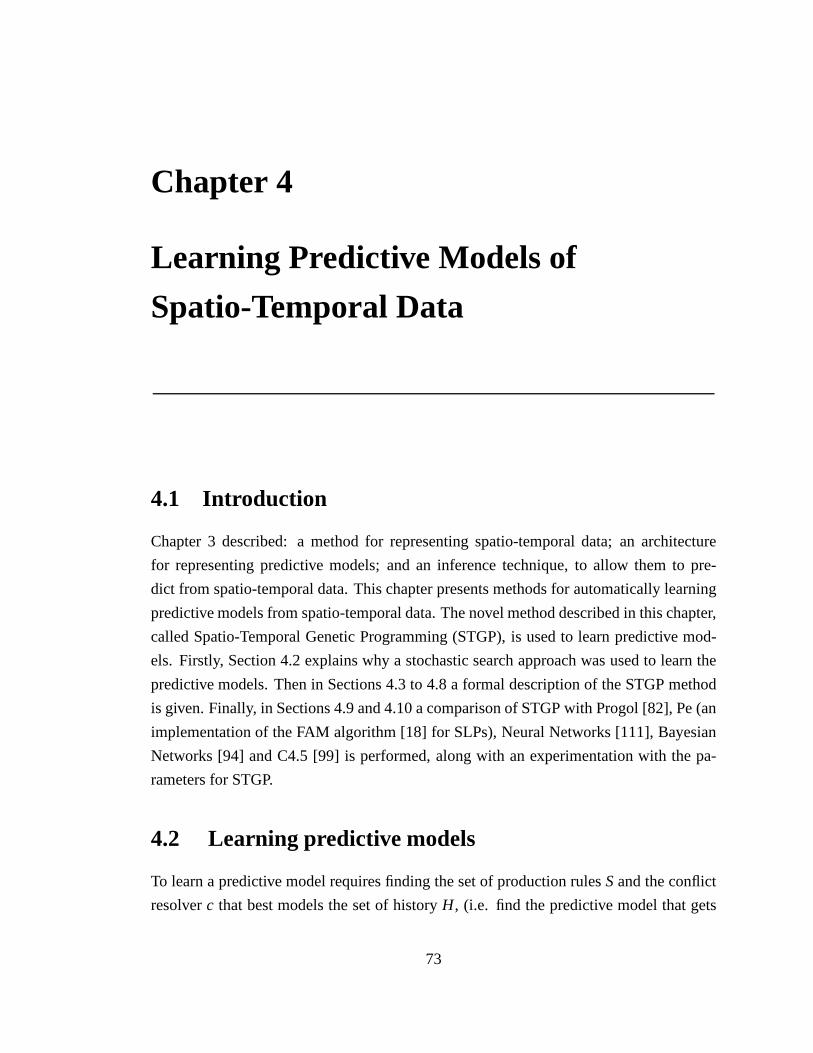
Chapter 4
Learning Predictive Models of
Spatio-Temporal Data
4.1 Introduction
Chapter 3 described: a method for representing spatio-temporal data; an architecture
for representing predictive models; and an inference technique, to allow them to pre-
dict from spatio-temporal data. This chapter presents methods for automatically learning
predictive models from spatio-temporal data. The novel method described in this chapter,
called Spatio-Temporal Genetic Programming (STGP), is used to learn predictive mod-
els. Firstly, Section 4.2 explains why a stochastic search approach was used to learn the
predictive models. Then in Sections 4.3 to 4.8 a formal description of the STGP method
is given. Finally, in Sections 4.9 and 4.10 a comparison of STGP with Progol [82], Pe (an
implementation of the FAM algorithm [18] for SLPs), Neural Networks [111], Bayesian
Networks [94] and C4.5 [99] is performed, along with an experimentation with the pa-
rameters for STGP.
4.2 Learning predictive models
To learn a predictive model requires finding the set of production rulesSand the conflict
resolverc that best models the set of historyH, (i.e. find the predictive model that gets
73

Chapter 4 Learning Predictive Models of Spatio-Temporal Data
the best accuracy when it predicts from the history) as shownin Equation 4.1.
argmaxS,c(P(S,c|H)) (4.1)
Predictive model learning in the context of this thesis can be broken down into two
parts: structure learning, and parameter learning [111]. Structure learning is on two lev-
els. Firstly, the optimal number of production rules needs to be found, and secondly the
optimal number of functions, variables, and constants, along with their connectivity needs
to be found for each production rule. Parameter learning involves computing a conditional
probability distribution for the conflict resolver (described in Section 3.3). This distribu-
tion does not contain any hidden variables, and the history data is complete, so there is a
closed form solution for calculating its parameters.
There are various approaches to perform structure and parameter learning. Section
2.5.1 reviewed different approaches to learning first orderlogic production rules, repre-
sented by Horn clauses. There were two main conclusions. Firstly, using stochastic or
evolutionary search finds good Horn clauses in a faster time than using greedy search
[4, 87, 122, 126, 129]. Secondly, learning a complete set of Horn clauses simultaneously
produces better results than sequentially learning a set ofHorn clauses [3,36,46,113,131].
These techniques have been incorporated into the approach described in this thesis: an
evolutionary search technique is used to learn the individual production rules and sets of
production rules simultaneously. Section 2.5.2 looked at techniques for learning the pa-
rameters of the conflict resolver. It was shown in [19,61] that learning both the production
rules, and the parameters together, rather than using a two stage process produced better
results. These ideas have again been introduced into the approach described in this the-
sis where both the production rules, and the parameters of the context chooser are learnt
simultaneously. The following section will give an overview of the approach.
4.3 Spatio-Temporal Genetic Programming
Figure 4.1 gives an overview of Spatio-Temporal Genetic Programming (STGP) the novel
method to learn the predictive models presented within thischapter. It is based on Ge-
netic Programming (GP), and uses the same set of steps that are used in GP, and Genetic
Algorithms (GA). The numbered set of steps below shows a run of STGP in more detail.
1. Initialise the structure of the predictive models: create a population of predictive
models which each contain a randomly generated number of production rules.
74

Chapter 4 Learning Predictive Models of Spatio-Temporal Data
Figure 4.1: A flow chart showing the different steps in a run ofSTGP.
2. Compute parameters for the predictive models:For each predictive model the
parameters for its conflict resolver need to be computed fromthe history.
3. Compute fitness value for each of the predictive model:Use a fitness function to
assign a fitness value to each of the predictive models.
4. Check stopping criteria: Check if the run has reached the maximum number of
generations allowed, or there is a predictive model in the population which has an
optimal fitness score. If so stop the run, and return the predictive model with the
best (maximal) fitness score.
5. Apply structure altering operations to the population of predictive models:
Apply structure altering operators to the population of predictive models to try and
improve their fitness.
6. Go back to step 2.
The following sections will explain these steps in more detail. Firstly, Section 4.4
describes the structure learning techniques including: initialisation techniques, and struc-
ture altering operators. Next, Section 4.6 shows the parameter learning technique. Finally,
Section 4.7 describes the fitness function.
75

Chapter 4 Learning Predictive Models of Spatio-Temporal Data
4.4 Initialising the population of predictive models
To initialise STGP a population of randomly generated predictive models is produced.
The process of generating a predictive model involves randomly creating a new produc-
tion rule. To create a new production rule involves randomlygenerating its condition, and
action sections. It is important that the population of predictive models is as diverse as
possible, as explained in Section 2.6.7. A population with high diversity initially provides
STGP with a wide range predictive models, which makes it morelikely it will find the
correct solution, and less likely to converge on a sub-optimal solution. Population diver-
sity and how it is affected by the different STGP parameters is explored in Section 4.10.3.
Initialisation of both the production rules and predictivemodels will now be described in
more detail.
4.4.1 Predictive model initialisation
Predictive models consist of a set of one or more production rules. When a new predic-
tive model is created, it is initialised with one randomly generated production rule. The
Ramped half and half method [58] (Section 2.6.2) is used to generate the condition sec-
tions of the production rules. This ensures that the population of predictive models has
production rules with condition sections that contain a variety of structures and depths.
4.4.2 Production rule initialisation
To create a new production rule involves firstly randomly creating the condition section,
and then randomly creating the action section.
4.4.2.1 Condition section initialisation
Section 3.3.1.1 showed how the condition section is defined.It contains a set of functions,
a set of variables, and a set of constants arranged in a Directed Acyclic Graph (DAG).
Two things are required to create a new condition section: firstly a method to constrain
the structure of the DAG so that it is always valid; and secondly a technique which uses
the structural constraints to build a valid condition section.
Given a set of functions, constants and variables there is a large number of DAG
structures that can be formed. However, not all structures will be valid, and these cannot
be evaluated on a particular history. Figure 4.2 shows two invalid condition sections.
The first condition section is evaluating whether the symbolRed is less than the symbol
Green; and the second condition section is evaluating if thenumber 1 is equal to the
76

Chapter 4 Learning Predictive Models of Spatio-Temporal Data
symbol Green. To solve this problem constraints are placed on the composition of the
DAG. This ensures that all DAG structures are evaluable, gives a good initial start point
to the structure learning algorithm, and reduces the searchspace of possible structures.
Strongly Typed Genetic Programming [79] is used to control the structure of the DAG.
It assigns a type to every function, constant, variable and function argument. A DAG is
only “valid” if for every function used in the DAG its argument types match the types of
its parent nodes. The possible types used in this thesis are:Int, Float, String, Boolean, or
Time.
Red
Less Than
Green 1 Green
Equal
Figure 4.2: Invalid condition sections.
The structural constraints described are used when generating a new condition section.
The user defines a maximum depth of the DAG. This allows the maximum complexity and
time to evaluate the condition section to be controlled. There are two possible ways to
build the condition section: the Full method, and the Grow method [58]. This thesis will
use the versions of the Full and Grow methods from [79], wherethe root node of the DAG
must have a Boolean type. Two changes are made to these methods so that they can be
used to produce production rules.
Firstly, if a function requires a variable as an argument STGP must use an existing
one, or generate a new one of the correct type. The entity or relation type of the variable
is defined in the sub-type of the argument. Firstly, STGP checks to see if there are any
variables matching the desired entity or relation type. If there is a set of variables, then
STGP can either decide to pick a random variable, or to generate a new variable. The
likelihood of picking an existing variableP(t) is shown in Equation 4.2. The equation
makes it increasingly hard to generate new variables as the number of them increases.
P(t) =Nt
Nt +1(4.2)
A new variable is generated when the maximum number of variables for a specific type
has not been exceeded. This limits the complexity of the condition section, and prevents
77

Chapter 4 Learning Predictive Models of Spatio-Temporal Data
STGP from producing predictive models that are overly complex. To generate a new
variable requires completing its entity type, and time range. The time will be randomly
chosen from either AllTime, Period time, or Point time. For Point and Period time, a time
range is also randomly generated. Period time is not used in any of the runs in this thesis,
but a discussion is given about how it could be used at the end of Chapter 5.
Secondly, to prevent condition sections from being generated that always evaluate
true (or false) a restriction is added to the Grow, and Full methods. This occurs when
the condition section contains sub-trees that either just contain constant value terminals,
or variables which are the same. When nodes are assigned to a function’s arguments a
check is performed to make sure they are not all constant value symbols, or use the same
variable. If this is the case another assignment is found.
An example of the Full method will now be shown, based on the Uno example from
Section 3.3. The following functions will be used:And (having a Boolean type, and a
Boolean type for the its arguments),Get-Colour (having a String type, and an argu-
ment containing a variable of type Card),Equal (having a Boolean type, and a String
type for its arguments), andNot Equal (having a Boolean type, and a String type for
its arguments). The following terminals will be usedRed, Green, andYellow . All the
terminals have a String type. The variables will all be of type Card. The stages of the ex-
ample are shown in Figure 4.3. The maximum depth is set to 3. The Full method initially
picks a function with a Boolean type. There are three possible options:And, Equal,
andNot Equal; andAnd is chosen. The type forAnd’s arguments is Boolean, and as
the method is not at the maximum depth a function with a Boolean type is chosen; this
time it is Equal . The argument type forEqual is String, and as the method is now
at the maximum depth only terminals of type String can be chosen. Get-Colour and
Red are chosen.Get-Colour also requires a variable, in this case the variablex of type
Card is used. Next, the second argument for theAnd node is found, andNot Equal is
selected. Again the argument type for theNot Equal node is String and as the method
is at the maximum depth only terminals of type String can be picked.Get-Colour and
Yellow are selected. Again,Get-Colour requires a variable this time the variabley
of type Card is used.
The functions and terminals which can be used in the condition section must be de-
fined before STGP is run. These can be manually defined, or generated from the property,
entity, or relation definitions. Some of the functions and terminals (described in Section
3.3.1.1) need extra parameters when they are defined. The Getfunction needs to have the
entity type, property, and attribute it will use. The Existsfunction needs to have the entity
or relation type. The Symbol terminal needs the symbol it will use. The Numeric terminal
78

Chapter 4 Learning Predictive Models of Spatio-Temporal Data
Red
Equal
And
ColourGet
x y
EqualNot
ColourGet
And
NotEqualEqual
Get
x y
Colour Red ColourGet
Yellow
And And
Equal
And
Equal
Red
And
x
Equal
ColourGet
Red
EqualNot
And
Red
Equal
x
ColourGet
Figure 4.3: An example condition section produced using theFull method.
needs the number it will use.
4.4.2.2 Action section initialisation
To generate a new action section STGP selects a random entity, or relation definition, then
for each property selects either a random number; symbol; oran existing variable in the
condition section, and property to use.
4.5 Altering the predictive models
A set of structure altering operators is used to modify the current set of predictive models,
to create a new population of predictive models. A population sampling method is used to
select predictive models from the current population. In this thesis tournament selection
and roulette wheel are used, as described in Section 2.6.4. These predictive models are
then altered either by modifying which production rules areused in the predictive models,
or by modifying the structure of the individual production rules in the predictive models.
Then the predictive models are added to the new population. This is shown in Figure 4.4.
79

Chapter 4 Learning Predictive Models of Spatio-Temporal Data
Figure 4.4: A flow chart showing the possible ways to alter thepredictive models in thecurrent population to produce a new population.
The following sections will explain how the predictive models and the production rules
are altered in more detail.
4.5.1 Altering the set of production rules
There are four kinds of operators to change the set of production rules in the predictive
models. These are:reproduction, addingin a new production rule,replacingan existing
production rule, andremovinga production rule. A set of probabilities are used to control
how much each operator is used. Which operator is used is selected randomly based
on a probability distributionPo. The operators have been inspired by Koza’s work on
architecture altering operations [59], as described in Section 2.6.6. The operators will
now be described in more detail.
Reproduction copies the predictive models unchanged into the new population.
Adding in a production rule from another predictive model This requires two predic-
tive models. A production rule from the first picked predictive model is randomly
selected, and added to the second. This second predictive model is then included in
the new population.
Replacing a production rule This requires two predictive models. A production rule
from the first predictive model is replaced by a production rule randomly selected
80

Chapter 4 Learning Predictive Models of Spatio-Temporal Data
from the second. The first predictive model is then included in the new population.
Removing a production rule A randomly selected production rule is removed from a
predictive model. The predictive model is then included in the new population.
4.5.2 Altering the composition of the individual production rules
Two operators are used to change the composition of individual production rules,crossover
andmutation[58].
4.5.2.1 Crossover
Crossover is used to swap over parts of two different production rules. Two kinds of
crossover are used with the production rules: condition section crossover, and action
section crossover.
Condition section crossover uses the condition sections oftwo production rules and
is based on the crossover technique used in [79]. To perform crossover a random node
in the first condition section is selected. The same probabilities as used in [58] are used
to select nodes in the DAG. With probability of 10% a terminalnode is picked, and with
probability of 90% a function node is picked. Nodes in the second condition section
which match the node’s type and sub-type are then found. If there are no matching nodes
then a new node in the first condition section is selected, andthe process repeats. When a
set of matching nodes in the second condition section has been found, a node in this set is
randomly selected. The node and its sub-tree in the first condition section is then swapped
with the selected node and its sub-tree in the second condition section. This can be seen
in Figure 4.5.
In action section crossover, if the action sections are bothentities or both relations
then entity or relation crossover can be performed. To perform entity crossover a random
property from the entity’s definition is selected, and then arandom attribute from the
property is selected. Then the values from each of these attributes in each entity are
swapped over. In relation crossover one of the entity types used in the relation’s definition
is chosen. Then the id value for this entity type within each relation is swapped over. If
one action section is a relation and the other is an entity then the action sections are just
swapped over.
81

Chapter 4 Learning Predictive Models of Spatio-Temporal Data
Crossover
Condition section 1 Condition section 2
Figure 4.5: The genetic operator Crossover being performedon two condition sections.
4.5.2.2 Mutation
There are two possible types of mutation used in this thesis:condition section mutation
and action section mutation. Condition section mutation, is based on the mutation op-
erator described in [79]. It selects a random node within thecondition section of the
production rule and replaces it and its children with a randomly generated DAG which
has a root node that matches the type of the randomly picked node. The Grow method is
used to produce the new DAG. The DAG’s depth is randomly chosen such that it does not
exceed the maximum depth of the DAG. Figure 4.6 shows a node (highlighted in black)
being selected, and a new DAG replacing it and its children. In action section mutation
a random property is selected from the entity and its value isreplaced with a randomly
generated value.
4.6 Conflict resolver parameter learning
Once a set of production rules have been produced the next stage is to compute the pa-
rameters for the conflict resolver. It is represented by a discrete conditional probability
distributionP(U |R), as described in Section 3.3. The distribution probabilistically decides
which set of enabled production rules should be fired to produce a prediction.
Calculation ofP(U |R) has a simple closed form solution and is computed in two
stages. Firstly evaluate each of the production rules at each point in the history. Secondly
fire the action sections of each enabled production rule. Then record which of the outputs
successfully matched the actual output at the next point in the history. The probability
82

Chapter 4 Learning Predictive Models of Spatio-Temporal Data
Mutation
Condition section
Figure 4.6: The genetic operator Mutation being performed on a condition section.
distribution can be computed as shown in Equation 4.3 by recording the number of times
(Nr ) the set of production rules have been enabled, or not enabled r = (r1, ..., rN), r i ∈
{true, f alse} when applied to the history; and the number of times (Nur) when the action
sections of the enabled production rules were fired their outputs matched the actual output
at the next time stepu = (u1, ...,uN), ui = {true, f alse}, ui is true if there is a match and
false otherwise.
P(U = u|R= r) =P(U = u,R= r)
P(R= r)=
Nur
Nr(4.3)
The probability distribution is computed over all occurring combinations of enabling/not
enabling the production rules, and output matches/mismatches. In theory this could be
large, but in practice the number of combinations is limited, so sparse storage solutions
can be used. The method used to compare the output from a production rule with the
actual outputH is described by Equation 4.4. It finds the entity or relationh from the
actual output that best matches the production rule output.The matching is done using
the Match function (shown in Figure 4.7) which computes the proportion of properties in
the entity or relation which have the same values to the output from the production rule.
MS(p,H) = maxh∈H(match(p,h)) (4.4)
The computation forP(U |R) can now be described more formally. At each pointt in
the historyH the set of production rulesSare evaluated and the resultsr are stored where
r i is true if the condition sectionbi of production rulei entails the subset of the training
83

Chapter 4 Learning Predictive Models of Spatio-Temporal Data
Input: Entity or relation (O) produced from the action section of aproduction rule and an entity or relation (C) from the history to compare it to.Output:The fraction of properties that match.
Function Match
If O andC have the same typesForeachpropertyp in O
If O andC have the same value for propertyps= s+ 1
t = t + 1Return s / t
ElseReturn 0
Figure 4.7: The pseudo code for the matching algorithm.
datah (biθT |= h) whereh∈ H, and false otherwise. The algorithm described in Section
3.4 is used to find the substitution (θT ) that causes the condition section of the production
rule to entail a subset of the history. Next, the firing setu is formed whereui = true if
biθT |= h andMS(aiθT) = 1; and false otherwise. Finally the number of times in the
historyNr a specificr occurs is computed, and the number of timesNur a specificr occurs
and specificu also occurs is computed, and used to computeP(U |R) (Equation 4.3).
1
32
Figure 4.8: A path containing three sensors numbered 1, 2 and3.
Parameter learning will be illustrated with an example. Figure 4.8 show a path which
has 3 sensors on it numbered 1, 2 and 3. People walk along the path passing over sensor
1, and then either take the left or right fork, passing over sensor 2 or 3 in the process. We
do not consider any other routes in this simplified example. Figure 4.9 shows a predictive
model for predicting which sensor the person will pass over next once they have passed
over sensor 1. Production rule 1 states that sensor 2 will detect next, and production rule
2 states that sensor 3 will detect next. The problem now is to learn the parameters of the
84

Chapter 4 Learning Predictive Models of Spatio-Temporal Data
R1: IF DETECT(SENSOR1, T) THEN DETECT(SENSOR2, T+1)R2: IF DETECT(SENSOR1, T) THEN DETECT(SENSOR3, T+1)
Figure 4.9: The predictive model for the Path example.
Time 1 2 3 4 5 6 7 8Detection history {1} {2} {1} {3} {1} {2} {1} {2}
r1 T F T F T F T Fr2 T F T F T F T Fu1 T F F F T F T Fu2 F F T F F F F F
Table 4.1: The prediction results for the Path model on a set of history. The history at eachpoint in time represents the sensor numbers that have been detected. There is only onedetection at each point in time because the condition sections of both of the productionrules only use detections at the current time.
conflict resolver for this predictive model. Table 4.1 showshow the model evaluated on a
history representing a sequence of sensor detections: 1, 2,1, 3, 1, 2, 1, 2 (this represents
4 people walking along the path, and 3 people taking the left fork, and 1 person taking the
right fork).
There are three possible situations that have occurred in this history, and these will be
used to compute the probability distributionP(U |R):
1. Both production rules are enabled on the history, but onlythe output of production
rule 1 matches the next detection (i.e. sensor 2 next), so only its action section
should be fired. This occurs at time points: 1, 5, and 7.
P(u1 = t,u2 = f |r1 = t, r2 = t) =Nu1=t,u2= f ,r1=t,r2=t
Nr1=t,r2=t=
34
= 0.75 (4.5)
2. Both production rules are enabled on the history, but onlythe output of production
rule 2 matches the next detection (i.e. sensor 3 next), so only its action section
should be fired. This occurs at time point 3.
P(u1 = f ,u2 = t|r1 = t, r2 = t) =Nu1= f ,u2=t,r1=t,r2=t
Nr1=t,r2=t=
14
= 0.25 (4.6)
3. None of the production rules were enabled on the history, and no output is predicted,
so none of the action sections should be fired. This occurs at time points: 2, 4, 6
and 8.
85

Chapter 4 Learning Predictive Models of Spatio-Temporal Data
P(u1 = f ,u2 = f |r1 = f , r2 = f ) =Nu1= f ,u2= f ,r1= f ,r2= f
Nr1= f ,r2= f=
44
= 1 (4.7)
There are other possible combinations, but these do not occur and so are not com-
puted. This means out of a possible 16 combinations (4 enabled combinations * 4 fired
combinations), only 3 are actually computed and stored.
4.7 Fitness function for scoring predictive models
The fitness function is used to produce a fitness score which represents how well a predic-
tive model predicts a future set of history from a past set of history. To compute the fitness
score the predictive model is applied at each point in the history to produce a prediction.
This prediction is compared against the history at the next time point to produce a pre-
dictive match score. The fitness score is calculated by computing the average predictive
match score over the history.
More formally given a predictive modelM and a set of historyH the predictive model
predicts from the historyH1:t at each time pointt. This is performed by the prediction
function described in Section 3.4 producing a set of predicted outputsW. Each pre-
dicted outputwi is a tuple(oi, pi) containing the outputoi , and its likelihoodpi . Equa-
tion 4.9 shows how the set of predicted outputs is compared with history at the next
time stepHt+1. To perform this comparison eachoi is compared againstHt+1 using the
FindBestMatch function (described below) and the result multiplied bypi . The best
comparison score is then returned. This process repeats over the entire history, and the
average comparison score is computed as shown in Equation 4.8.
f (M,H) =1|H|
∗∑t
compare(predict(M,H1:t),Ht+1) (4.8)
compare(W,D) = Maxi(l i ∗FindBestMatch(pi,D)) (4.9)
TheFindBestMatch function (shown in Figure 4.10) takes the actual history, and
the predicted output, and firstly pads each of them out with blank entities or relations so
that they are the same size. Then, for each item in the actual history, a unique match in
the predicted output is found. For each of the matches a comparison is done between the
two objects using the Match algorithm described in Section 4.6. An exhaustive search is
then performed over all the possible combination of matchesto find the best (maximal)
matching score.
86

Chapter 4 Learning Predictive Models of Spatio-Temporal Data
Input: A set of Entity or relations (P) predicted by the predictive model,a set of entities or relations (H) describing history data at the next time point.Output:The score on how well the prediction matches the history data.
Function FindBestMatch
Fill the setsP andH with empty entities or relations such that they are the same length.best= 0Foreachmappingm from objects inP to objects inH
s= 0Foreachobjectp in P get its mapped objectm(p)
s= s + Match(p, m(p))If s> best
best= sReturn best
Figure 4.10: The pseudo code for theFindBestMatch algorithm.
The fitness function will now be illustrated with an example.We will use the same
predictive model, and conflict resolver from the previous section. This time the predictive
model is applied to a different set of history as shown in Table 4.2. In theW row each
tuple is the predicted sensor number, followed by its probability for example(2,0.75) is
the prediction that Sensor 2 will detect next with the probability of 0.75. The underscore
for the sensor number represents that there was no output. The bold items show which
of the predicted outputs match the actual outputs. In thecomparerow the 1 in each
calculation is the result from the compare function and shows that the predicted output
exactly matched the actual output. The fitness score can thenbe computed as shown in
Equation 4.10.
f =(1∗0.75)+0+(1∗0.25)+0+(1∗0.25)+0
6= 0.208 (4.10)
4.8 Controlling the size of the predictive models
To prevent the predictive models from overfitting the history, and getting too large, some
form of size control is required. In GP this is called bloat and refers to excess code in the
program trees that are not used. The Tarpeian method [22] is one of the methods in GP
used to control bloat. It has been shown to perform well on standard GP datasets [67],
therefore will be used in STGP to control the size of the predictive models. This method is
described in Section 2.6.7. Section 4.10.3.2 shows resultson how changing the Tarpeian
value affects STGP.
87

Chapter 4 Learning Predictive Models of Spatio-Temporal Data
Time 1 2 3 4 5 6Detection history {1} {2} {1} {3} {1} {3}
r1 t f t f t fr2 t f t f t fW {(2,0.75), {( ,1)} {(2,0.75), {( ,1)} {(2,0.75), {( ,1)}
(3,0.25)} (3,0.25)} (3,0.25)}compare 1*0.75 0 1*0.25 0 1*0.25 0
Table 4.2: The fitness results for the Path predictive model on a set of history data. Vari-ablesr1 andr2 represents that production rule 1 or 2 were enabled or not enabled on thehistory. VariableW represents the set of predictions, which each tuple is a prediction froma production rule containing an output, and its probability. The tuples in bold representwhere the prediction matches the detection at the next time step. The variablecomparerepresents how well the prediction matched the actual history.
4.9 Evaluation
A comparison was performed with STGP and five other methods: Progol [82], Pe (an
implementation of the FAM algorithm [18] for SLPs), Neural Networks [111], Bayesian
Networks [94] and C4.5 [99]. Five datasets were used for the comparison: Uno, Uno2,
Paper Scissors Stone (PSS), CCTV and Play Your Cards Right (PYCR). Three of the
datasets (Uno, Uno2, and PSS) were taken from the work of Needhamet al. [89]. The
other two datasets (CCTV and PYCR) are novel, and were produced for this thesis. Both
of these datasets are non-deterministic and test how the different methods deal with learn-
ing from non-deterministic data. PYCR was also set as a grandchallenge in the work
of [89].
Section 4.9.1 will describe these datasets in more detail. Some of the datasets have
training sets that are generated from video, Section 4.9.2 will describe how this was per-
formed. Finally, Section 4.9.3 describes the representation used for each of the methods.
4.9.1 Overview of the datasets
This section gives a brief overview of the datasets: Uno, Uno2, PSS, PYCR, and CCTV.
4.9.1.1 Uno and Uno2
The card game Uno involves two players. Firstly one player says “Play” to signify both
players should put down a card. Each player then puts down a card, and the first player
who correctly shouts out how the two cards match picks up all the cards that have been
88

Chapter 4 Learning Predictive Models of Spatio-Temporal Data
put down. If the cards both have the same picture, and colour then “Same” should be
shouted out. If the cards have the same picture, but different colours then “Shape” should
be shouted out. If the cards have the same colour, but different pictures then “Colour”
should be shouted out. Finally, if the two cards are different then “Nothing” is said. This
process repeats until a player cannot put down a card.
The game Uno2 works in a very similar manner; the only difference is that instead of
one player saying “Play” and both players putting down a card, they just take it in turns to
put a card down. The similarity is then based on the current and previous cards that were
put down. The methods should learn predictive models from the Uno and Uno2 datasets
that given the cards put down by each of the players should predict the result that should
be said.
For both Uno and Uno2 six training sets were produced. One wasfrom real world
video, as described in Section 4.9.2.1. This contained 50 rounds of the game for both
Uno and Uno2. The rest were hand crafted with different levels of noise. The noise levels
were: 0% (clean), 5%, 10%, 20% and 30%. The noise was producedby changing or
removing the speech outputs, or removing cards. The datasets contained 130 rounds of
the game.
4.9.1.2 Papers scissors stone
Paper Scissors Stone is a card game again played by two people, each with three cards
representing paper, scissors and stone. One player will say“Play”, and a card is selected
by each player. Both cards are placed down face up at the same time. The game is played
from the view point of player 1. If player 1’s card beats player 2’s card then “Win” will
be heard. If player 1’s card is beaten by player 2’s card then “Lose” will be heard. If both
players have put down the same cards then it is declared a drawand “Draw” will be heard.
Scissors will beat paper; paper beats stone; and stone beatsscissors. Table 4.3 shows the
possible states.
(Player 1) Paper Scissors Stone
(Player 2) Paper Draw Loose WinScissors Win Draw LooseStone Loose Win Draw
Table 4.3: The result states for a game of Paper Scissors Stone between two players.
Again, the methods should learn predictive models that given the cards put down by
each of the players should predict the result that should be said. Six training datasets
were produced in a similar manner to Uno and Uno2. One datasetwas generated from
89

Chapter 4 Learning Predictive Models of Spatio-Temporal Data
real-world video, and the rest were handcrafted with the same levels of noise as the Uno
and Uno2 datasets. The real world video training set contained 100 rounds of the game,
and the handcrafted training sets contained 130 rounds of the game.
4.9.1.3 CCTV data of a path
A static camera was used to film a scene containing a path with ajunction point in it. A
frame of the video is shown in Figure 4.11(a), and Figure 4.12shows the four possible
movement patterns in the scene. The video is used to mockup a set of CCTV cameras
over the image as shown in Figure 4.11(b).
Figure 4.11: Figure (a) shows a frame of the video with a person taking a decision at thejunction point. Figure (b) shows the possible location of the virtual CCTV cameras in theimage.
Figure 4.12: The four possible movement patterns in the CCTVscene.
The methods should learn a predictive model that can predictbased on the CCTV cam-
eras a person has been in previously which CCTV camera they will appear in next. The
CCTV dataset tests if the different methods can learn from, and model, non-deterministic
90

Chapter 4 Learning Predictive Models of Spatio-Temporal Data
data. Six training sets were produced in the similar manner to the PSS, Uno and Uno2
datasets. One dataset was produced from real-world video, and the rest were handcrafted.
The same noise levels as previously described were used. Noise was added by removing
regions and changing their numbers. The real world dataset contained 50 detections, and
the handcrafted datasets contained around 120 detections.
4.9.1.4 Play your cards right
Play Your Cards Right (PYCR) is a card game played by a person and a dealer. The cards
are numbered from 1 to 5 with 1 being the lowest, and 5 being thehighest. Firstly the
dealer says “Play” and puts down a card face up. Then the person must say if they predict
the next card will be “Higher” or “Lower” than this card. The dealer will then put down
the next card. If the person guesses correctly then the dealer says “Win”, otherwise they
will say “Lose”.
The methods should learn a predictive model that should use the state of the cards
put down to predict the spoken outcomes from the person and the dealer. PYCR, like
the CCTV dataset tests if the different methods can learn from non-deterministic spatio-
temporal data. Five handcrafted training sets were produced, having the same noise levels
as the previous datasets. The noise was added by removing cards and speech outputs, and
changing the speech outputs. The datasets contained 130 rounds of the game.
4.9.2 Spatio-temporal data acquisition
Four out of the five datasets (Uno, Uno2, PSS and CCTV) have a training set that is
generated from video. Firstly, spatio-temporal data must be acquired from the videos,
and then it must be represented within the different methods. This section describes data
acquisition, and the next section describes data representation.
4.9.2.1 Uno, Uno2 and PSS
The Uno, Uno2 and PSS videos will be that used in [89]. The datafiles from this paper are
used for the experiments in this chapter, but the speech cluster labels are changed to be the
actual speech (word) labels. The remainder of this section will explain how the datafiles
were produced. The videos were taken of the game playing area, and objects moving in
the area were tracked using a generic blob tracker [68]. Whenan object was stationary
for a number of frames it is assumed to be part of the game. Features from the object
including texture (calculated from Gabor wavelets, and Gaussians applied at various ori-
entations and scales), colour (calculated from a binned histogram of hue, and saturation),
91

Chapter 4 Learning Predictive Models of Spatio-Temporal Data
and position were produced. Each colour, and texture feature was independently clustered
using agglomerative clustering. A graph was produced with data items as the nodes, and
the feature clusters used to weight the edges. The graph was then partitioned to form
clusters of data items. These clusters were then used to train a vector quantisation based
nearest neighbour classifier. One of the players had their voice recorded during the games.
The energy of the speech signal was analysed using a fixed length window. When the en-
ergy was over a fixed threshold spectral analysis was performed on the window, and a
histogram of the result was produced. K-means clustering was then performed on the
speech samples, to find clusters of similar speech sounds. Inthis thesis the previous step
is changed by replacing the speech cluster labels by manually annotating them with the
actual speech (word) labels.
4.9.2.2 CCTV
A 10 minute video of people walking along a path containing a junction was filmed. This
was then used to mock up a network of CCTV cameras. Figure 4.11shows a frame from
the video. Virtual motion detectors, representing CCTV cameras, were hand placed over
the video (Figure 4.11 right). Using frame differencing, and morphological operations the
video was processed to determine the location of the motion.If the number of moved pix-
els in a region exceeded a fixed threshold then the virtual detector outputted that motion
had occurred at that location. To prevent false detections the motion detection is imple-
mented as a 2-state machine (where the states are motion/no motion). The state machine
required a number of frames (normally 10) of stability to change state.
4.9.3 Representation
This section will show how the spatio-temporal data is represented in the different meth-
ods.
4.9.3.1 Progol and Pe
In Progol a set of events occurring in a visual scene is represented as a sequence of states
in which each state describes: the current state of the objects in the scene; an action associ-
ated with this state; the time the state occurs at; and how thestate relates to previous state.
Progol requires four elements as its input: a set of types; some background knowledge;
some examples; and a set of mode declarations. The Uno dataset will be used to illustrate
these elements. The rest of the datasets use similar elements. The same representation
from [89] will be used for the Uno, Uno2 and PSS datasets.
92

Chapter 4 Learning Predictive Models of Spatio-Temporal Data
Firstly, Progol needs some type declarations. Figure 4.13 shows the type declarations
for the Uno dataset: texture, colour, position, and speech.No background information is
required for any of the datasets.
texture(f0). texture(f1). texture(f2).colour(c0). colour(c1). colour(c2).position(p0). position(p1).speech(s_1). speech(s_2). speech(s_3).speech(s_4). speech(s_5). speech(s_6).speech(s_7). speech(s_8). speech(s_9). speech(s_10).
Figure 4.13: Type declarations for Progol on the Uno dataset.
Secondly, Progol requires a set of examples – Figure 4.14 shows some examples for
the Uno dataset. The first example shows two cards being placed in the scene, and an
appropriate response (action) being heard. The second example shows an empty scene,
and an appropriate action being heard. Both examples have a similar structure. Thetime
predicate represents the time the example occurred at. Thesuccessor predicate repre-
sents how this example temporally relates to a previous example. Thestate predicate
is used to represent the visual scene. It either represents an empty scene, as shown in Ex-
ample 2, represented by[], or it represents a set of objects in the scene. In Example 1 the
state of the world is:[f1,c0,p0],[f0,c0,p1] which represents two objects, one
with texturef1 and colourc0, at positionp0; and the other with texturef0 and colour
c0, at positionp1. Finally theaction predicate represents what spoken response has
been heard.
Finally, Progol requires some mode declarations. Figure 4.15 shows the mode decla-
rations for the Uno dataset. It shows that Progol needs to produce a clause which has an
action term its head, and its body can contain the termssuccessor andstate.
To convert the clauses learnt by Progol into a Stochastic Logic Program (Section
2.5.3.3) the likelihood of each clause needs to be calculated from data. Two approaches
are used in this thesis to do this. Firstly, Pe (which implements the failure-adjusted max-
imisation algorithm from [18]) is used. Secondly, the clauses learnt by Progol are con-
verted into a predictive model, and the parameters of its conflict resolver are estimated by
STGP. This is performed by converting each Horn clause into aproduction rule, where
the action section contains the appropriate entity or relation representing the head of the
Horn clause, and the condition section represents the body of the Horn clause. Then,
the algorithm described in Section 4.6 is used to estimate the parameters of the conflict
resolver.
93

Chapter 4 Learning Predictive Models of Spatio-Temporal Data
%Example 1time(t_0).time(t_15).successor(t_0,t_15).state([[f1,c0,p0],[f0,c0,p1]],t_15).action(s_10,t_15).
%Example 2time(t_15).time(t_20).successor(t_15,t_20).state([],t_20).action(s_9,t_20).
Figure 4.14: Examples of the Uno dataset which are used with Progol.
modeh(1,action(#speech,+time))modeb(*,state([[-texture,-colour,-position],
[-texture,-colour,-position]],+time))modeb(*,state([],+time))modeb(1, +any = #any)modeb(*,successor(-time,+time))
Figure 4.15: Mode declarations for Progol on the Uno dataset.
4.9.3.2 STGP
STGP requires the following: a set of property, entity and relation definitions; a datafile;
and a set of terminals, and functions. These will now be explained by using the Uno
dataset as an example. The other datasets use similar settings.
The representation used in the datafile is described in Section 3.2. The properties and
entities used to learn the Uno dataset are shown in Figure 4.16. There are four property
definitions: colour, texture, position, and speech, and twoentity definitions: card (with
properties: texture, colour and position), and action (with property speech).
Figure 4.17 shows the terminals used to learn the Uno dataset. There are colour sym-
bolsc0, c1; texture symbolsf0, f1, f2; position symbolsp0, p1; and speech symbols
Same, Shape, Nothing, Play, Colour. Figure 4.18 shows the functions used to
learn the Uno dataset. There are functions to check the existence of a card, or a talker
entity in the worldExists(Card), Exists(Action). Also, there are functions
to get property information from the cards, and talker entitiesGet(Card:Colour),
94

Chapter 4 Learning Predictive Models of Spatio-Temporal Data
Get(Card:Position), Get(Card:Texture), Get(Action:Speech). Fi-
nally, there are functions to compare symbolic dataEqual, Not-Equal,and logical
functionsAnd, Or, Not.
<PROPERTY-DEFINITION NAME="COLOUR"><ATTRIBUTE NAME="NAME" TYPE="SYMBOLIC" VALUES="c0,c1,c2"/>
</PROPERTY-DEFINITION>
<PROPERTY-DEFINITION NAME="TEXTURE"><ATTRIBUTE NAME="NAME" TYPE="SYMBOLIC" VALUES="f0,f1,f2"/>
</PROPERTY-DEFINITION>
<PROPERTY-DEFINITION NAME="POSITION"><ATTRIBUTE NAME="NAME" TYPE="SYMBOLIC" VALUES="p0,p1"/>
</PROPERTY-DEFINITION>
<PROPERTY-DEFINITION NAME="SPEECH"><ATTRIBUTE NAME="NAME" TYPE="SYMBOLIC"
VALUES="Shape,Colour, Nothing,Same,Play"/></PROPERTY-DEFINITION>
<ENTITY-DEFINITION NAME="CARD"><LEARNABLE VALUE="FALSE"/><PROPERTY NAME="COLOUR"/><PROPERTY NAME="POSITION"/><PROPERTY NAME="TEXTURE"/>
</ENTITY-DEFINITION>
<ENTITY-DEFINITION NAME="ACTION"><LEARNABLE VALUE="TRUE"/><PROPERTY NAME="SPEECH"/>
</ENTITY-DEFINITION>
Figure 4.16: Properties, and entity definitions for STGP on the Uno dataset.
c0, c1p0, p1f0, f1, f2Same, Shape, Nothing, Play, Colour
Figure 4.17: Terminals for STGP used to learn the Uno dataset.
95

Chapter 4 Learning Predictive Models of Spatio-Temporal Data
Exists(Card), Exists(Action),Get(Card:Colour), Get(Card:Position)Get(Card:Texture), Get(Action:Speech)And, Or, Not-Equal, Equal, Not
Figure 4.18: Functions used to learn the Uno dataset
4.9.3.3 Bayesian Networks, Neural Networks, and C4.5
These methods were implemented using the WEKA machine learning system [41]. This
requires a fixed length representation to describe the datasets. The representation will de-
scribe the current state of the scene, along with an associated action that needs to be learnt.
Figure 4.19 shows an example representation for the Uno dataset. The first six attributes
(Colour1, Position1, Texture1, Colour2, Position2, andTexture2) de-
scribe the properties of the cards in the scene, withcN, pN, fN representing that no card
is present. The final attribute (Speech) represents the action associated with the scene.
The first line of data indicates that no cards are in the scene and that play (s_play) was
uttered. The second line of data represents that a card with colourc2, positionp0, and
texturef0, and a card with colourc2, positionp1, and texturef1 are in the scene and
that colour (s_colour) was said.
@RELATION Uno@ATTRIBUTE Colour1 {c0,c1,c2,cN}@ATTRIBUTE Position1 {p0,p1,pN}@ATTRIBUTE Texture1 {f0,f1,f2,fN}@ATTRIBUTE Colour2 {c0,c1,c2,cN}@ATTRIBUTE Position2 {p0,p1,pN}@ATTRIBUTE Texture2 {f0,f1,f2,fN}@ATTRIBUTE Speech {s_shape,s_play,s_same,s_colour,
s_nothing,s_unknown}@DATAcN,pN,fN,cN,pN,fN,s_playc2,p0,f0,c2,p1,f1,s_colour
Figure 4.19: An example Uno dataset representation for Bayesian Networks, Neural Net-works, and C4.5.
96

Chapter 4 Learning Predictive Models of Spatio-Temporal Data
4.10 Results
This section will firstly outline the evaluation criteria for the experiments. Then an analy-
sis of the results from the different methods, and experiments with the different parameters
for STGP will be presented.
4.10.1 Evaluation criteria
Two criteria were used to evaluate the predictive models produced by the different meth-
ods: coverage, and accuracy. Coverage (c) scores if the predictive model can correctly
predict the history (i.e. the probability of correct prediction is greater than 0) and is the
number of correct predictions (nc) divided by the history size (s) (Equation 4.11). Accu-
racy (a) scores with what probability the correct prediction is made. It is calculated by
taking the sum of the likelihoodsl = {l1, ..., lnc} for each correct prediction, and divid-
ing it by the history size, as shown in Equation 4.12. In non-deterministic scenarios this
cannot be 100%.
c =nc
s(4.11)
a =∑ l is
(4.12)
4.10.2 A comparison of STGP with current methods
Figures 4.20 - 4.27 show graphs comparing the coverage and accuracy of STGP with
Bayesian Networks, C4.5, Neural Networks, and Progol on thefive different datasets ex-
plained in Section 4.9.1. The graphs also show the results for estimating the probabilities
of the clauses learnt by Progol using Pe, and STGP. Ten fold cross validation was used
in all the experiments. In STGP the training folds are used inthe following way: four
folds are used to estimate the parameters of the conflict resolver, and five folds are used
to score the predictive models. A windowed section (which moves at every generation)
of the parameter fold, and the scoring fold is used for the calculations. Overall the results
show that STGP had accuracy on all the datasets that was as good as, or better than the
other methods.
On both Uno and Uno2 the maximum achievable result for these datasets was 100%
accuracy, and 100% coverage (as they are deterministic). Itcan be seen in Figures 4.20
and 4.21 that STGP matches the expected result for the clean dataset, and keeps close
to this result with noisy data. Combining Progol with STGP onboth the Uno and Uno2
datasets produced more accurate results than all methods other than STGP. The Uno and
97

Chapter 4 Learning Predictive Models of Spatio-Temporal Data
Uno2 datasets do not contain enough examples to describe every possible outcome that
can occur within the game. C4.5, Neural Networks, and Bayesian Networks cannot pro-
duce generalised rules from the examples, and effectively rely on storing common exam-
ples and their outcomes. They fail to get 100% accuracy and 100% coverage (Figures
4.20 and 4.21), as they will have not learnt enough examples to correctly predict from all
the test data. These methods are also affected by noise in theexamples, which can be seen
in the graphs. Progol and STGP which can learn generalised rules from the examples get
better results because the generalised rules can still correctly predict test examples which
have not occurred in the training data. Progol suffers from aclause evaluation problem
that affects its coverage and accuracy results. This is caused by an incorrect ordering of
the clauses it has learnt. As explained in Section 2.5.2 the clauses are applied in the order
they are learnt until one clause entails the unseen example.In this thesis the clauses were
applied in the order that Progol had learnt them. This often means that although Progol
had learnt the correct set of clauses their ordering caused Progol to predict incorrectly.
Figure 4.22 shows one of the results from the Uno Clean dataset. It can be shown that the
correct number of clauses has been learnt, but when they are applied to the test fold it got
93% coverage and 93% accuracy. If the clauses were in the correct order it would have
got 100% coverage and 100% accuracy. The problem is due to where the Same clause is
located. In Figure 4.22 the Colour and Shape clauses are applied before the Same clause
which means Progol will incorrectly predict a same event as acolour or shape event. By
placing the Same clause above the Colour and Shape clauses this problem is solved, as
shown in Figure 4.23.
Pe can be used to solve this clause ordering problem. It estimates the likelihood that
a clause is used in a prediction. All the clauses are applied to the unseen example, and
the likelihood of a prediction is based on the clauses that entail the unseen example. This
approach improves Progol’s coverage results, but does not improve its accuracy due to
some clauses clashing when they entail an unseen example. For example, the estimated
probabilities from Pe for the clauses in Figure 4.22 are shown in Figure 4.24.
Using these probabilities the likelihood of the Same clauseentailing an unseen exam-
ple is based on the Same clause likelihood along with the likelihood of the Colour, Shape,
and Nothing clauses because these also entail the unseen example. The probability of
predicting the next event will be same is then 0.050.1+0.1+0.05+0.23 = 0.1. However, if the
Shape, Colour and Nothing clauses were not included in the prediction, the prediction for
same would have the correct probability of 1.0. Pe must output all clauses that match the
data, unlike STGP which can prevent the action sections of some production rules from
being output. This can be seen in the results as combining theclauses learnt by Progol
98

Chapter 4 Learning Predictive Models of Spatio-Temporal Data
0
20
40
60
80
100
Bayes Net.C4.5 NN Progol Progol+ Pe
Progol+ STGP
STGP
Mea
n C
over
age
(%)
Method
Uno - Clean
0
20
40
60
80
100
Bayes Net.C4.5 NN Progol Progol+ Pe
Progol+ STGP
STGP
Mea
n A
ccur
acy
(%)
Method
Uno - Clean
0
20
40
60
80
100
Bayes Net.C4.5 NN Progol Progol+ Pe
Progol+ STGP
STGP
Mea
n C
over
age
(%)
Method
Uno - 10% Noise
0
20
40
60
80
100
Bayes Net.C4.5 NN Progol Progol+ Pe
Progol+ STGP
STGP
Mea
n A
ccur
acy
(%)
Method
Uno - 10% Noise
Figure 4.20: The mean accuracy and coverage for Uno Clean (top) and Uno 10% noise(bottom). The error bars show one standard deviation from the mean. All results wereproduced by 10 fold cross validation.
with STGP gets more accurate results than Progol, and Progolcombined with Pe.
On the PSS dataset the optimal obtainable result is again 100% coverage, and 100%
accuracy (as it is deterministic). STGP, as shown in Figure 4.25, gets the best accuracy
results, and matches the optimal result on the clean dataset, and keeps close to this for
the noisy datasets. C4.5 gets the same accuracy results as STGP on the clean dataset,
but its accuracy reduces on the noisy datasets. Neural networks get good results (average
accuracy 97%) on the clean datasets, but again this drops on the noisy datasets. Progol,
Progol combined with Pe, and Progol combined with STGP got worse results than C4.5
and Neural Networks. The PSS datasets, however, are different to Uno and Uno2 in that
no general rules are required to get good results on the training examples. The training
data contain all the possible combinations of the game, so all that is required is to memo-
rise these combinations. This explains why C4.5 and Neural Networks gets better results
on this dataset than on the Uno and Uno2 datasets. Progol again suffers from the clause
ordering problem described previously which affects its results. Pe solves the clause or-
dering problem, but the clashing clauses reduce the accuracy of the results. When the
clauses from Progol are combined with STGP there is not enough training data to cor-
99

Chapter 4 Learning Predictive Models of Spatio-Temporal Data
0
20
40
60
80
100
Bayes Net.C4.5 NN Progol Progol+ Pe
Progol+ STGP
STGP
Mea
n C
over
age
(%)
Method
Uno2 - Clean
0
20
40
60
80
100
Bayes Net.C4.5 NN Progol Progol+ Pe
Progol+ STGP
STGP
Mea
n A
ccur
acy
(%)
Method
Uno2 - Clean
0
20
40
60
80
100
Bayes Net.C4.5 NN Progol Progol+ Pe
Progol+ STGP
STGP
Mea
n C
over
age
(%)
Method
Uno2 - 10% Noise
0
20
40
60
80
100
Bayes Net.C4.5 NN Progol Progol+ Pe
Progol+ STGP
STGP
Mea
n A
ccur
acy
(%)
Method
Uno2 - 10% Noise
Figure 4.21: The mean accuracy and coverage for Uno2 Clean (top) and Uno2 10% noise(bottom). The error bars show one standard deviation from the mean. All results wereproduced by 10 fold cross validation.
action(s_play,A) :- state([],A).action(s_colour,A) :- state([[B,C,D],[B,E,F]],A).action(s_shape,A) :- state([[B,C,D],[E,F,D]],A).action(s_same,A) :- state([[B,C,D],[B,E,D]],A).action(s_nothing,A) :- state([[B,C,D],[E,F,G]],A).
Figure 4.22: A result for Progol on the Uno dataset with the clauses in the wrong order.
action(s_play,A) :- state([],A).action(s_same,A) :- state([[B,C,D],[B,E,D]],A).action(s_colour,A) :- state([[B,C,D],[B,E,F]],A).action(s_shape,A) :- state([[B,C,D],[E,F,D]],A).action(s_nothing,A) :- state([[B,C,D],[E,F,G]],A).
Figure 4.23: A result for Progol on the Uno dataset with the clauses in the correct order.
rectly estimate the parameters for the conflict resolver. This prevents it from correctly
predicting all of the test data, which reduces its accuracy.
On the PYCR dataset STGP gets the best accuracy and coverage as shown in Figure
100

Chapter 4 Learning Predictive Models of Spatio-Temporal Data
0.50::action(s_play,A) :- state([],A).0.10::action(s_colour,A) :- state([[B,C,D],[B,E,F]],A).0.10::action(s_shape,A) :- state([[B,C,D],[E,F,D]],A).0.05::action(s_same,A) :- state([[B,C,D],[B,E,D]],A).0.23::action(s_nothing,A) :- state([[B,C,D],[E,F,G]],A).
Figure 4.24: The estimated probabilities for the clauses inFigure 4.22 using Pe.
0
20
40
60
80
100
Bayes Net.C4.5 NN Progol Progol+ Pe
Progol+ STGP
STGP
Mea
n C
over
age
(%)
Method
PSS - Clean
0
20
40
60
80
100
Bayes Net.C4.5 NN Progol Progol+ Pe
Progol+ STGP
STGP
Mea
n A
ccur
acy
(%)
Method
PSS - Clean
0
20
40
60
80
100
Bayes Net.C4.5 NN Progol Progol+ Pe
Progol+ STGP
STGP
Mea
n C
over
age
(%)
Method
PSS - 10% Noise
0
20
40
60
80
100
Bayes Net.C4.5 NN Progol Progol+ Pe
Progol+ STGP
STGP
Mea
n A
ccur
acy
(%)
Method
PSS - 10% Noise
Figure 4.25: The mean accuracy and coverage for PSS Clean (top) and PSS 10% noise(bottom). The error bars show one standard deviation from the mean. All results wereproduced by 10 fold cross validation.
4.26. The optimal result for PYCR is 100% coverage, and 90% accuracy (as it has non-
deterministic outcomes). This is based on playing the game where each possible game
combination occurs in equal proportion. STGP is close to this for both the clean and noisy
datasets. It does fail to get 100% coverage due to not learning rules for infrequent events
in the training data. On the clean data, Bayesian Networks, C4.5 and Neural Networks
got more accurate results than Progol, and Progol combined with Pe. However, on the
noisy data the inverse is true, as can be seen in Figure 4.26.
Progol does not learn enough clauses to cover the possible cases in the game. When
Progol is combined with either Pe, or STGP the accuracy does not improve due to the lack
101

Chapter 4 Learning Predictive Models of Spatio-Temporal Data
of correct clauses. Progol’s fitness function is based on howwell the clauses cover rather
than predict the data. It looks at the number of positive examples to negative examples
covered by a potential clause. The more negative examples a clause covers, the less likely
Progol will be to use it. This can make it hard to learn clausesfrom non-deterministic data,
where a particular state in the world can have multiple outcomes. If insufficient examples
are available Progol sees multiple outcomes as noise, whichcan prevent it finding a clause.
0
20
40
60
80
100
Bayes Net.C4.5 NN Progol Progol+ Pe
Progol+ STGP
STGP
Mea
n C
over
age
(%)
Method
PYCR - Clean
0
20
40
60
80
100
Bayes Net.C4.5 NN Progol Progol+ Pe
Progol+ STGP
STGP
Mea
n A
ccur
acy
(%)
Method
PYCR - Clean
0
20
40
60
80
100
Bayes Net.C4.5 NN Progol Progol+ Pe
Progol+ STGP
STGP
Mea
n C
over
age
(%)
Method
PYCR - 20% Noise
0
20
40
60
80
100
Bayes Net.C4.5 NN Progol Progol+ Pe
Progol+ STGP
STGP
Mea
n A
ccur
acy
(%)
Method
PYCR - 20% Noise
Figure 4.26: The mean accuracy and coverage for PYCR Clean (top) and PYCR 20%noise (bottom). The error bars show one standard deviation from the mean. All resultswere produced by 10 fold cross validation.
The results for the CCTV dataset are shown in Figure 4.27. Theexpected results
for CCTV are 100% coverage and 83% accuracy (as it has non-deterministic outcomes).
This is based on the four actions from Figure 4.12 occurring in equal proportions in the
data. STGP got the best results, but does not get 100% coverage, because it fails to learn
infrequent changes between regions in the training data. InSTGP for a predictive model
to match a particular pattern in the training data the pattern must occur both within the
window used the estimate the parameters of the conflict resolver, and in the window to
score the predictive models. This is done to prevent STGP from learning from noise, and
to help it generalise. Infrequent region changes that only appear in one of the windows
will not be modelled, and are seen as noise. This is why some ofthe infrequent region
102

Chapter 4 Learning Predictive Models of Spatio-Temporal Data
changes in the CCTV dataset were not modelled. This can be verified in the results as the
predictive models learnt from different folds modelled different actions. Neural Networks,
and Progol got results that were statistically the same on the clean dataset. Bayesian
Networks, C4.5 and Progol combined with Pe got the worst results on the clean dataset.
The methods get similar results with increasing levels of noise, except for STGP, and
Progol combined with STGP. Progol fails to get good results,because the CCTV dataset is
non-deterministic which affects its fitness function (explained previously). When Progol
is combined with Pe accuracy is not improved. This is due to problems with clashing
clauses, which effect Pe’s accuracy. By combining Progol with STGP its accuracy results
are improved, and they are shown to be statistically similarto STGP (p-value on clean
data is 0.03, with 5% noise is 0.0003, and with 10% noise is 0.01).
0
20
40
60
80
100
Bayes Net.C4.5 NN Progol Progol+ Pe
Progol+ STGP
STGP
Mea
n C
over
age
(%)
Method
CCTV - Clean
0
20
40
60
80
100
Bayes Net.C4.5 NN Progol Progol+ Pe
Progol+ STGP
STGP
Mea
n A
ccur
acy
(%)
Method
CCTV - Clean
0
20
40
60
80
100
Bayes Net.C4.5 NN Progol Progol+ Pe
Progol+ STGP
STGP
Mea
n C
over
age
(%)
Method
CCTV - 20% Noise
0
20
40
60
80
100
Bayes Net.C4.5 NN Progol Progol+ Pe
Progol+ STGP
STGP
Mea
n A
ccur
acy
(%)
Method
CCTV - 20% Noise
Figure 4.27: The mean accuracy and coverage for CCTV Clean (top) and CCTV 20%noise (bottom). The error bars show one standard deviation from the mean. All resultswere produced by 10 fold cross validation.
4.10.3 Parameter experimentation with STGP
This section presents results from experimenting with the different STGP parameters to
see how they affect its performance on different datasets. The initial values for the param-
103

Chapter 4 Learning Predictive Models of Spatio-Temporal Data
eters are shown in Table 4.4, these were based on typical parameter values from the GP
literature. The rest of this section will show experiments varying each of the parameters
in turn. The best results from each experiment are used in subsequent experiments.
Parameter ValuePopulation Size 6000Tarpeian value None
Maximum number of generations 100Initialisation generations 10
Selection method Tournament selection using 6 individualsPercentage of operators Reproduction (10%), Delete (10%),
in initialisation generations Adding (40%), Replace (40%)Percentage of operators Reproduction (10%), Crossover (50%),in normal generations Mutation (10%), Delete (10%),
Adding (10%), Replace (10%)Conflict resolver type Probabilistic
Table 4.4: Initial settings for STGP.
4.10.3.1 Population Size
The following values were used for the population size parameter: 1000, 2000, 3000,
4000, 5000, and 6000. Figure 4.28 show the accuracy results on the clean versions of
the datasets. The graphs show that by increasing populationsize this is not a statistically
significant change in the average accuracy of the results. Similar results were seen on the
medium and high noise datasets. The PSS and Uno2 clean datasets have a large amount of
variance in the accuracy results for population size 1000, when compared with the other
population sizes. To increase population diversity, and provide STGP with a greater range
of predictive models when trying to find a solution it was decided to keep the population
size at 6000 for all the datasets in this chapter. This allowsSTGP to deal with noisy
datasets, and makes it more likely to converge to the correctsolution.
4.10.3.2 Tarpeian value
In the population size experiments there were no constraints on the possible size of the
predictive models. Figure 4.29 shows that the average size of the predictive models across
all datasets typically increased a constant rate to the number of generations STGP had
performed. This relationship is the same regardless of population size, and shows the
predictive models suffer from bloat. As explained in Section 2.6.7 bloat causes the pre-
dictive models to contain redundant elements which could make them less general, and
104

Chapter 4 Learning Predictive Models of Spatio-Temporal Data
94
95
96
97
98
99
100
101
102
0 1000 2000 3000 4000 5000 6000 7000
Mea
n A
ccur
acy
(%)
Population Size
PSS - Clean
98.4
98.6
98.8
99
99.2
99.4
99.6
99.8
100
100.2
100.4
0 1000 2000 3000 4000 5000 6000 7000
Mea
n A
ccur
acy
(%)
Population Size
Uno - Clean
88
90
92
94
96
98
100
102
104
0 1000 2000 3000 4000 5000 6000 7000
Mea
n A
ccur
acy
(%)
Population Size
Uno2 - Clean
74
76
78
80
82
84
86
88
0 1000 2000 3000 4000 5000 6000 7000
Mea
n A
ccur
acy
(%)
Population Size
CCTV - Clean
83
84
85
86
87
88
89
90
91
92
93
94
0 1000 2000 3000 4000 5000 6000 7000
Mea
n A
ccur
acy
(%)
Population Size
PYCR - Clean
Figure 4.28: The mean accuracy graphs for population size onthe clean datasets. Theerror bars show one standard deviation from the mean. All results were produced by 10fold cross validation.
slow down STGP’s search for a solution. To control bloat the Tarpeian method [22] was
used. The amount of bloat control is based on the Tarpeian value that varies from 1 to
10. Two experiments were then performed. The first experiment applied Tarpeian bloat
control over the entire run using the Tarpeian values in the integer range of 1 to 10. The
second experiment delaying the Tarpeian bloat control until after the 10 initialisation gen-
erations had been performed, to see if the increased diversity in the initial generations of
the run would produce better results.
To find the best Tarpeian value for each dataset requires finding the lowest value which
105

Chapter 4 Learning Predictive Models of Spatio-Temporal Data
0
20
40
60
80
100
120
140
160
180
200
220
0 20 40 60 80 100 120
Mea
n S
ize
Generations
Uno - 0% Noise
100020003000400050006000
0
50
100
150
200
250
300
0 20 40 60 80 100 120
Mea
n S
ize
Generations
Path - 0% Noise
100020003000400050006000
Figure 4.29: The mean predictive model size for the CCTV (right) and Uno (left).
has an accuracy at least as good as the accuracy for the dataset with no Tarpeian control.
This means finding on the accuracy graph the point where the mean accuracy begins to
flatten out.
Figure 4.30 shows the accuracy values for the Tarpeian values on the clean datasets.
Figure 4.31 shows the average model size for the different Tarpeian values. It can be seen
that for CCTV and Uno2 a Tarpeian value of 3 will produce results with the same accu-
racy as without using bloat control, but the size of the predictive models is significantly
reduced. For Uno and PYCR this value is 4, and for PSS this value is 5. PSS requires a
more complex predictive model than the rest of the datasets which explains in its higher
Tarpeian value. For all datasets a Tarpeian value of 2 did notget good accuracy results
when compared to the accuracy results to not using bloat control. The medium noise
accuracy results for the datasets show a similar picture. The accuracy results on the high
noise datasets show they require slightly different Tarpeian values. PSS, Uno2, CCTV
and PYCR require a Tarpeian value of 4; and Uno requires a Tarpeian value of 6.
Figures 4.32 and 4.33 show the accuracy and size results on the clean datasets when
the Tarpeian bloat control is not performed for the initial 10 generations. It can be seen
that there is no significant difference in the results when compared with using Tarpeian
bloat control for the entire run. The same findings are found on the medium, and high
noise datasets. It was therefore decided to apply Tarpeian bloat control for the entire
length of the run.
The Tarpeian method controls the size of the population, which affects its diversity.
The results show that a very low Tarpeian value decreases thediversity of the population
too much, and prevents STGP from finding the correct solution. The datasets which
require simpler predictive models like Uno, and Uno2 require a slightly lower Tarpeian
values than the datasets which require more complex predictive models like PSS. Chapter
7 presents an adaptive Tarpeian method that varies the Tarpeian value during the run
106
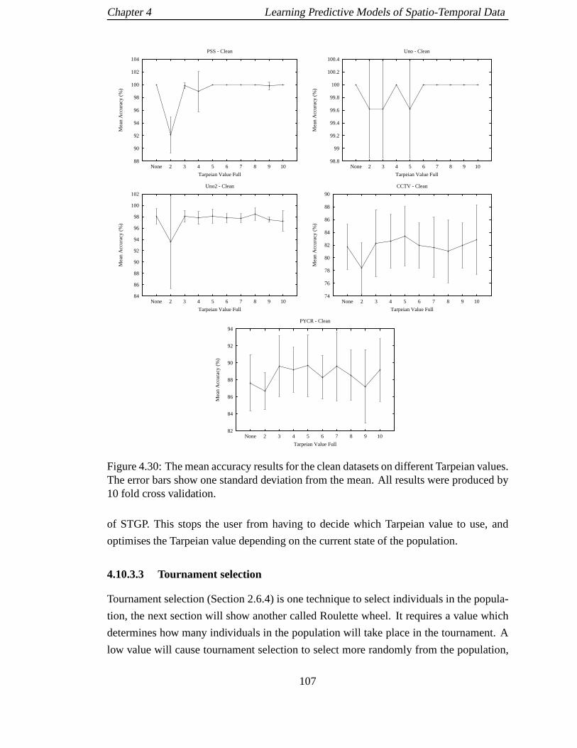
Chapter 4 Learning Predictive Models of Spatio-Temporal Data
88
90
92
94
96
98
100
102
104
1098765432None
Mea
n A
ccur
acy
(%)
Tarpeian Value Full
PSS - Clean
98.8
99
99.2
99.4
99.6
99.8
100
100.2
100.4
1098765432None
Mea
n A
ccur
acy
(%)
Tarpeian Value Full
Uno - Clean
84
86
88
90
92
94
96
98
100
102
1098765432None
Mea
n A
ccur
acy
(%)
Tarpeian Value Full
Uno2 - Clean
74
76
78
80
82
84
86
88
90
1098765432None
Mea
n A
ccur
acy
(%)
Tarpeian Value Full
CCTV - Clean
82
84
86
88
90
92
94
1098765432None
Mea
n A
ccur
acy
(%)
Tarpeian Value Full
PYCR - Clean
Figure 4.30: The mean accuracy results for the clean datasets on different Tarpeian values.The error bars show one standard deviation from the mean. Allresults were produced by10 fold cross validation.
of STGP. This stops the user from having to decide which Tarpeian value to use, and
optimises the Tarpeian value depending on the current stateof the population.
4.10.3.3 Tournament selection
Tournament selection (Section 2.6.4) is one technique to select individuals in the popula-
tion, the next section will show another called Roulette wheel. It requires a value which
determines how many individuals in the population will takeplace in the tournament. A
low value will cause tournament selection to select more randomly from the population,
107

Chapter 4 Learning Predictive Models of Spatio-Temporal Data
10
20
30
40
50
60
70
80
90
100
110
1098765432None
Mea
n S
ize
Tarpeian Value Full
PSS - Clean
10
20
30
40
50
60
70
80
1098765432None
Mea
n S
ize
Tarpeian Value Full
Uno - Clean
0
20
40
60
80
100
120
140
160
1098765432None
Mea
n S
ize
Tarpeian Value Full
Uno2 - Clean
0
20
40
60
80
100
120
140
160
180
200
220
1098765432None
Mea
n S
ize
Tarpeian Value Full
CCTV - Clean
0
50
100
150
200
250
300
350
1098765432None
Mea
n S
ize
Tarpeian Value Full
PYCR - Clean
Figure 4.31: The mean size results for the clean datasets on different Tarpeian values. Theerror bars show one standard deviation from the mean. All results were produced by 10fold cross validation.
and higher values will cause it to select more from the fitter individuals in the popula-
tion. To find the best value for the datasets an experiment wasperformed that tried out
the following tournament selection values: 2,5,10,20,40,60,80,100,120,140,160,180, and
200.
Figure 4.34 shows how the different tournament selection values performed on the
clean datasets. It can be seen that for the PYCR, Uno and PSS datasets an increased
tournament selection value reduces the mean accuracy of theresults (PSS p-value=0.004,
PYCR p-value=0.05, Uno p-value=0.03; calculations based on tournament values 5 and
108

Chapter 4 Learning Predictive Models of Spatio-Temporal Data
94
95
96
97
98
99
100
101
102
1098765432None
Mea
n A
ccur
acy
(%)
Tarpeian Value
PSS - Clean
99
99.5
100
100.5
101
1098765432None
Mea
n A
ccur
acy
(%)
Tarpeian Value
Uno - Clean
88
90
92
94
96
98
100
102
104
1098765432None
Mea
n A
ccur
acy
(%)
Tarpeian Value
Uno2 - Clean
72
74
76
78
80
82
84
86
88
90
1098765432None
Mea
n A
ccur
acy
(%)
Tarpeian Value
CCTV - Clean
84
85
86
87
88
89
90
91
92
93
1098765432None
Mea
n A
ccur
acy
(%)
Tarpeian Value
PYCR - Clean
Figure 4.32: The mean accuracy results for the clean datasets on different Tarpeian valueswhere Tarpeian bloat control starts after the first 10 generations. The error bars show onestandard deviation from the mean. All results were producedby 10 fold cross validation.
200). For the Uno2 and CCTV datasets a increased tournament selection value had no
statistically significant change in the accuracy in the results (Uno2 p-value=0.35, CCTV
p-value=0.43; calculations based on tournament values 5 and 200). Across all datasets a
tournament selection value of 2 produced poor results. A similar pattern can be seen as
with the medium noise datasets as with the clean datasets, with the exception that STGP
gets worse accuracy results on the Path dataset with an increasing tournament selection
value, and the accuracy results on the Uno dataset do not havea statistically significant
(p-value 0.64) change as the tournament selection value is increased. On the datasets with
109

Chapter 4 Learning Predictive Models of Spatio-Temporal Data
20
30
40
50
60
70
80
90
100
110
1098765432None
Mea
n S
ize
Tarpeian Value
PSS - Clean
10
20
30
40
50
60
70
80
1098765432None
Mea
n S
ize
Tarpeian Value
Uno - Clean
0
20
40
60
80
100
120
140
160
1098765432None
Mea
n S
ize
Tarpeian Value
Uno2 - Clean
0
20
40
60
80
100
120
140
160
180
200
220
1098765432None
Mea
n S
ize
Tarpeian Value
CCTV - Clean
0
50
100
150
200
250
300
350
1098765432None
Mea
n S
ize
Tarpeian Value
PYCR - Clean
Figure 4.33: The mean size results for the clean datasets on different Tarpeian valueswhere Tarpeian bloat control starts after the first 10 generations. The error bars show onestandard deviation from the mean. All results were producedby 10 fold cross validation.
high noise levels varying the tournament selection value has little change in the results
apart from for PYCR where it got worse accuracy with an increasing tournament selection
value. The variation in the results is due to population diversity. Larger tournament
selection values force STGP to sample more from the fitter individuals in the population,
which will reduce the population diversity. For some datasets like Uno, and Uno2 it has
been shown that solutions can still be found even with reduced population diversity, but
for the rest of the datasets this reduced diversity will not allow STGP to find the correct
solution. Small tournament selection values on the other hand increase the population
110

Chapter 4 Learning Predictive Models of Spatio-Temporal Data
88
90
92
94
96
98
100
102
104
50 100 150 200
Mea
n A
ccur
acy
(%)
Tournament Selection Value
PSS - Clean
80
85
90
95
100
105
50 100 150 200
Mea
n A
ccur
acy
(%)
Tournament Selection Value
Uno - Clean
80
85
90
95
100
105
50 100 150 200
Mea
n A
ccur
acy
(%)
Tournament Selection Value
Uno2 - Clean
72
74
76
78
80
82
84
86
88
90
50 100 150 200
Mea
n A
ccur
acy
(%)
Tournament Selection Value
CCTV - Clean
78
80
82
84
86
88
90
92
94
50 100 150 200
Mea
n A
ccur
acy
(%)
Tournament Selection Value
PYCR - Clean
Figure 4.34: The mean accuracy results for the clean datasets on different Tournamentselection values. The error bars show one standard deviation from the mean. All resultswere produced by 10 fold cross validation.
diversity, but force STGP to search randomly over the space of predictive models. This
random search will take longer time to find the correct solution, and often results in STGP
finding a locally optimal solution. A balance between using atournament selection value
which is too small, or too large needs to be found. It was decided to keep the tournament
selection value at 6 for all datasets in the remaining experiments, which is a reasonable
compromise based on the results shown.
111

Chapter 4 Learning Predictive Models of Spatio-Temporal Data
4.10.3.4 Roulette wheel
Roulette wheel selection (Section 2.6.4) is analogous to allocating space on a circular
wheel depending on each individuals fitness. A pointer is then virtually spun to select
individuals. Figure 4.35 shows graphs showing the results of Roulette wheel and Tour-
nament selection on the clean datasets. It can be seen that Roulette wheel selection does
not produce very accurate results for all datasets. This canbe explained in more detail
by looking at the best value for the generations, as shown in Figure 4.36. These graphs
show that the best score for the individuals using Roulette wheel either stays constant or
increases (when it should go down). This shows that Roulettewheel selection is selecting
too randomly from the population, and is not focusing on the fitter individuals in the pop-
ulation affecting the accuracy results. The same results can be seen on the medium noise
datasets. On the high noise datasets there is not any statistically significant difference
between Roulette wheel and Tournament selection on PYCR, and Uno2. It was decided
to keep tournament selection as the selection method due to its the better accuracy results
over Roulette wheel selection.
4.10.3.5 Maximum number of generations
To find out if increasing the maximum number of generations STGP is run for would
increase the accuracy of the results an experiment was performed. STGP was run with
the following values for the maximum number of generations:150, 200 and 250. For all
datasets there was no change in the results for by increasingthe generation value from
100 generations. Figure 4.37 shows the average best value for each generation for the
clean datasets It can be seen that STGP converges on a solution by 100 generations for
all datasets, and that the average best value does not changeby increasing the amount of
generations. This explains why running STGP for more generations does not increase the
accuracy of the results. A generation value of 100 was therefore chosen, to be used for all
datasets.
4.10.3.6 Operators
The final parameter to investigate was the operators used to evolve the predictive models.
In Table 4.4 the percentage of the adding and replacement operators is increased for the
first 10 generations. Then the percentage of these operatorswas reduced, and the percent-
age of the crossover operator is increased. The idea behind this approach is to initially
perform a global search to try and find the best number of production rules in the predic-
tive models. Then a local search is performed to try and locally optimise the predictive
112

Chapter 4 Learning Predictive Models of Spatio-Temporal Data
75
80
85
90
95
100
Roulette WheelTournament Selection
Mea
n A
ccur
acy
(%)
Selection Method
PSS - Clean
70
75
80
85
90
95
100
Roulette WheelTournament Selection
Mea
n A
ccur
acy
(%)
Selection Method
Uno - Clean
60
65
70
75
80
85
90
95
100
105
Roulette WheelTournament Selection
Mea
n A
ccur
acy
(%)
Selection Method
Uno2 - Clean
68
70
72
74
76
78
80
82
84
86
Roulette WheelTournament Selection
Mea
n A
ccur
acy
(%)
Selection Method
CCTV - Clean
55
60
65
70
75
80
85
90
Roulette WheelTournament Selection
Mea
n A
ccur
acy
(%)
Selection Method
PYCR - Clean
Figure 4.35: The mean accuracy results for the clean datasets on comparing Roulettewheel with Tournament selection. The error bars show one standard deviation from themean. All results were produced by 10 fold cross validation.
models. To see how this global search effects the results an experiment was performed. It
looked into varying the number of generations the global search was performed for. The
values were None, 10, 20, and 30.
Figure 4.38 shows the results on the clean datasets. STGP gotthe best score on Uno,
PYCR and PSS by using 10 generations of the global search phase. For Uno and PSS
STGP converged in half the number of generations by using 10 generations of the global
search phase than for any other value. STGP found the best solution on the Uno2 dataset
by using 20 generations of the global search phase. STGP converges on the solution for
113

Chapter 4 Learning Predictive Models of Spatio-Temporal Data
0.05
0.1
0.15
0.2
0.25
0.3
0.35
0.4
0.45
0 20 40 60 80 100 120
Mea
n B
est S
core
Generations
Uno2 - Clean
Tournament selectionRoulette wheel
0
0.05
0.1
0.15
0.2
0.25
0.3
0 20 40 60 80 100 120
Mea
n B
est S
core
Generations
Uno - Clean
Tournament selectionRoulette wheel
0.1
0.15
0.2
0.25
0.3
0.35
0 20 40 60 80 100 120
Mea
n B
est S
core
Generations
CCTV - Clean
Tournament selectionRoulette wheel
0.1
0.15
0.2
0.25
0.3
0.35
0.4
0 20 40 60 80 100 120
Mea
n B
est S
core
Generations
PYCR - Clean
Tournament selectionRoulette wheel
0
0.05
0.1
0.15
0.2
0.25
0.3
0 20 40 60 80 100 120
Mea
n B
est S
core
Generations
PSS - Clean
Tournament selectionRoulette wheel
Figure 4.36: The best fitness score for the predictive modelsfor the clean datasets usingRoulette wheel, and Tournament selection.
114

Chapter 4 Learning Predictive Models of Spatio-Temporal Data
0
0.05
0.1
0.15
0.2
0.25
0.3
0.35
0.4
0.45
0 50 100 150 200 250
Mea
n B
est S
core
Generations
Uno2 - Clean
100150200250
0
0.05
0.1
0.15
0.2
0.25
0.3
0 50 100 150 200 250
Mea
n B
est S
core
Generations
Uno - Clean
100150200250
0.1
0.15
0.2
0.25
0.3
0.35
0.4
0 50 100 150 200 250
Mea
n B
est S
core
Generations
CCTV - Clean
100150200250
0.05
0.1
0.15
0.2
0.25
0.3
0.35
0 50 100 150 200 250
Mea
n B
est S
core
Generations
PYCR - Clean
100150200250
0
0.05
0.1
0.15
0.2
0.25
0.3
0 50 100 150 200 250
Mea
n B
est S
core
Generations
PSS - Clean
100150200250
Figure 4.37: The best fitness score for the predictive modelsfor the clean datasets withdifferent values for the maximum number of generations.
115

Chapter 4 Learning Predictive Models of Spatio-Temporal Data
the CCTV dataset so long as some form of global search phase isused. By not using the
global search phase it can be seen that it takes STGP longer toconverge to a solution,
and on the Uno2 and PYCR datasets it fails to converge on the correct solution. Similar
comments can be applied to the results for the datasets with medium noise, as for the
clean datasets. STGP, however, converges fastest on the Uno2 dataset with a global search
period of 10 generations, but gets slightly better results with a global search period of 30
generations. A similar story can be applied to the results from the datasets with high
noise, apart from the Uno2 dataset the best global search period is 10 generations. For the
Uno2 dataset the best results are found with 20 generations for the global search period.
The results show that a period of increased adding and replacing of production rules in
the predictive models reduces the convergence time, and also makes it more likely to find
the correct solution. Solutions for the CCTV dataset can be found by just using global
search, but for the rest of the datasets a combination of the global search, and local search
are required to find the correct solution. This shows that forthe CCTV dataset all the
production rules required for the solution are generated inthe initial generation, and all
that is required is to find the correct combination of these production rules. For the rest of
the datasets finding the best combination of the production rules generated in the initial
generation allows STGP to find the correct area of the search space to locate the correct
solution. Then the crossover and mutation operators can be used to locally optimise the
production rules to find the correct solution.
The number of generations that the global search is performed for effects the number
of generations it takes STGP to convergence on the correct solution, and its ability to
find the correct solution. The results show that performing the global search for a larger
number of generations (e.g. 30) causes the value of the best predictive model to converge
during the global search, this value only starts to reduce when local search is performed.
Converging during the global search is bad for two reasons: it reduces the diversity in the
population, which might mean STGP will not find the correct solution; and it increases the
number of generations required to find the correct solution.The value of 10 generations
for the global search was chosen for all datasets.
4.10.4 Conflict resolver
The previous experiments all used the probabilistic conflict resolver described in Section
4.6. An experiment was performed to see what would happen if avery simple conflict
resolver was used, where every production rule that was enabled was fired to produce a
prediction. This was only performed on the deterministic datasets (Uno, Uno2, and PSS)
116

Chapter 4 Learning Predictive Models of Spatio-Temporal Data
0
0.05
0.1
0.15
0.2
0.25
0.3
0.35
0.4
0 20 40 60 80 100 120
Mea
n B
est S
core
Generations
Uno2 - Clean
1102030
0
0.05
0.1
0.15
0.2
0.25
0.3
0 20 40 60 80 100 120
Mea
n B
est S
core
Generations
Uno - Clean
1102030
0.1
0.15
0.2
0.25
0.3
0.35
0 20 40 60 80 100 120
Mea
n B
est S
core
Generations
CCTV - Clean
1102030
0.05
0.1
0.15
0.2
0.25
0.3
0.35
0 20 40 60 80 100 120
Mea
n B
est S
core
Generations
PYCR - Clean
1102030
0
0.05
0.1
0.15
0.2
0.25
0.3
0 20 40 60 80 100 120
Mea
n B
est S
core
Generations
PSS - Clean
1102030
Figure 4.38: The fitness score results for the best scoring predictive models for the cleandatasets where the number of generations performed on the global search is increased.
117

Chapter 4 Learning Predictive Models of Spatio-Temporal Data
as the conflict resolver is unable to deal with non-deterministic data. The experiment was
the same as the Tarpeian value experiments from Section 4.10.3.2. Figures 4.39 and 4.40
show the results on the clean datasets. It can be seen that theaccuracy results on both:
using bloat control for the entire run, and delaying bloat control by 10 generations is sig-
nificantly worse than the accuracy results using a probabilistic conflict resolver (Section
4.10.3.2). These results showed that when a probabilistic conflict resolver was used the
accuracy was close to 100% on the clean datasets. Similar results were observed on the
medium and high noise datasets. For these reasons it was decided to use the probabilistic
conflict resolver for all the datasets in this chapter.
The reason why the predictive models using the simple conflict resolver performed
poorly (in terms of both coverage and accuracy) is down to onereason: a more complex
search space. The search space when using the simple conflictresolver is full of local
optima compared to one where a probabilistic conflict resolver is used. The search space
contains many predictive models where the only way to get into the fitter part of the search
space is to firstly find a less fit area of the search space. This is because to improve the
fitness of a predictive model it must go through two states. Firstly some of its production
rules must be enabled at the same time, but when fired they produce different predictions,
which causes a conflict. Then the predictive model has to evolve to resolve this conflict.
When the sub-models are conflicting the predictive model gets a lower fitness score than
it currently has. Once the conflict has been resolved the predictive model gets a higher
fitness score. STGP probabilistically selects fitter predictive models for use in the next
population. This can mean that the evolution can get stuck ina local optima where the
predictive models containing conflicting production rulesare never picked and the run
locally converges.
4.11 Conclusions
This chapter has described Spatio-Temporal Genetic Programming (STGP). This is used
to learn the predictive models as described in Chapter 3. It has been compared with Pro-
gol, Neural Networks, Bayesian Networks, and C4.5; on five different datasets. Three
were deterministic, and two were non-deterministic. STGP got the best results overall.
Progol suffered from a clause clashing problem that effected both its coverage and accu-
racy. When Progol was combined with Pe it managed to improve Progol’s coverage, but
due to clashing clauses it does not improve its accuracy. Combining Progol with STGP
improved both Progol’s coverage and accuracy on all datasets. Bayesian Networks and
C4.5 performed fairly well, but were limited due to their inability to learn generalised
118

Chapter 4 Learning Predictive Models of Spatio-Temporal Data
78
80
82
84
86
88
90
92
1098765432None
Mea
n A
ccur
acy
(%)
Tarpeian Value
PSS - Clean
-20
0
20
40
60
80
100
120
140
160
180
1098765432None
Mea
n S
ize
Tarpeian Value
PSS - Clean
82
83
84
85
86
87
88
89
90
91
92
93
1098765432None
Mea
n A
ccur
acy
(%)
Tarpeian Value
Uno - Clean
0
10
20
30
40
50
60
1098765432None
Mea
n S
ize
Tarpeian Value
Uno - Clean
62
64
66
68
70
72
74
76
78
80
82
1098765432None
Mea
n A
ccur
acy
(%)
Tarpeian Value
Uno2 - Clean
-20
-10
0
10
20
30
40
50
60
1098765432None
Mea
n S
ize
Tarpeian Value
Uno2 - Clean
Figure 4.39: The mean accuracy and size results for the cleandatasets on differentTarpeian values where Tarpeian bloat control starts after the first 10 generations, and asimple conflict resolver is used in the predictive models. The error bars show one stan-dard deviation from the mean. All results were produced by 10fold cross validation.
rules from data.
STGP produces the best results with: some form of size control on the predictive
models; the tournament selection sampling technique usinga tournament selection value
that favours the better scoring predictive models; and an increased amount of adding and
replacement of production rules in the initial 10 generations of the run. The results on the
maximum number of generations showed that STGP had converged on a solution by 100
generations. Work could be done to investigate diversity techniques (Section 2.6.7) to see
119

Chapter 4 Learning Predictive Models of Spatio-Temporal Data
78
80
82
84
86
88
90
92
94
1098765432None
Mea
n A
ccur
acy
(%)
Tarpeian Value Full
PSS - Clean
-10
0
10
20
30
40
50
60
70
80
90
1098765432None
Mea
n S
ize
Tarpeian Value Full
PSS - Clean
80
82
84
86
88
90
92
94
96
98
1098765432None
Mea
n A
ccur
acy
(%)
Tarpeian Value Full
Uno - Clean
-10
0
10
20
30
40
50
60
70
80
90
100
1098765432None
Mea
n S
ize
Tarpeian Value Full
Uno - Clean
64
66
68
70
72
74
76
78
80
82
1098765432None
Mea
n A
ccur
acy
(%)
Tarpeian Value Full
Uno2 - Clean
-20
-10
0
10
20
30
40
50
60
1098765432None
Mea
n S
ize
Tarpeian Value Full
Uno2 - Clean
Figure 4.40: The mean accuracy and size results for the cleandatasets on differentTarpeian values where a simple conflict resolver is used in the predictive models. Theerror bars show one standard deviation from the mean. All results were produced by 10fold cross validation.
if maintaining diversity for a larger number of generationsimproves the results.
120

Chapter 5
Learning Predictive Models Using A
Qualitative Representation of Time
5.1 Introduction
In Chapter 4 the predictive models used a sequential approach for representing time. This
is not very robust to noise and the presence of multiple objects, for reasons which will
be discussed in Section 5.2. This chapter describes the use of qualitative relations to
represent time, which solves this problem. Four novel temporal state relations are de-
scribed, shown in Section 5.4. Section 5.6 firstly presents acomparison of STGP, with:
Progol [82], Neural Networks [111], Bayesian Networks [94]and C4.5 [99] on learn-
ing predictive models containing temporal relations from an Uno dataset, and a CCTV
dataset. Secondly, to see how the temporal relations allow apredictive model to deal with
noise, and multiple objects the STGP results on the CCTV dataset from this chapter, and
Chapter 4 are applied to two CCTV test sets one containing multiple people, and one
containing random injection noise. Thirdly, results with experimenting with some of the
parameters for STGP is presented.
121

Chapter 5 Learning Predictive Models Using A Qualitative Representation of Time
5.2 Quantitative representation of time
Section 2.4.2.2 described Markovian approaches to temporal modelling include Variable
Length Markov Models (VLMMs) [35] and Markov Chains. Each observation represents
a state of the world at a specific time. The sequence of observation vectors are used to
predict the most likely subsequent observations. Our work in Chapter 4 followed this
principle: the variables in the condition section used a relative Point time representation
to reference entity and relationship instances in the history. There are two main issues
with this implicit representation of time. Firstly, when there is injection noise occurring
in the data (i.e. noise occurs as extra items between the dataitems), and secondly when
there are multiple objects in the scene. These both cause thesequence ordering to change.
Any predictive models that rely on an explicit observation sequence ordering will then
fail to recognise the observations, and will be unable to make a prediction.
To illustrate the problems with the sequential representation of time we take an ex-
ample inspired by the CCTV domain in Chapter 4. Figure 5.1 shows a crossroads. On
the crossroads are five circular regions numbered 1 to 5. Whenmotion is detected in a
region, the region will produce an output. An arrow represents a person walking through
the crossroads going through regions 1, 2 and then 3. The motion through the crossroads
can be represented using continuous time as shown in the graph in Figure 5.1. To be
able to use this data with a sequential representation of time it must be converted into an
observation sequence. This is normally done by temporal quantisation. There are two
possible approaches: sample from the data at a fixed rate, or compress each of the con-
stant property time ranges into a single sample, by samplingat one point per time range
(for example the end, or start time) illustrated in Figure 5.1. Fixed sampling produces a
far more detailed representation of the data, but often contains large amounts of repeated
data. Compressing the time ranges reduces the amount of information that is represented
(for example the length and absolute start and end times are lost), but it is a more compact
representation which can be easier to learn from due to its lower complexity.
Figure 5.2 shows how injection noise might affect a predictive model. The same
person is walking through the crossroads passing through regions 1, 2, and 3, but this
time region 4 outputs incorrectly (for example due to cameranoise). This can be seen
as injection noise occurring between region detections at locations 1 and 2 in both the
continuous time graph and in the observation sequence. Thismay cause problems if the
model relies on an observation sequence occurring in a fixed ordering.
Figure 5.3 shows the same crossroads, but now two people are walking through at the
same time. It will be used to show how multiple objects in the scene might affect the pre-
122

Chapter 5 Learning Predictive Models Using A Qualitative Representation of Time
1
t − 2 t − 1 t
2 3
Continuous time
Quantised time
Reg
ion
Time
2
3
1
Time
Mov
emen
t
2
3
54
1
Figure 5.1: This diagram shows a person walking along a crossroads and passing throughthe circular regions numbered 1, 2 and 3. The movement in the scene is representedas a continuous time graph. Temporal quantisation is applied to the graph to produce asequence of region detections.
Mov
emen
t
Continuous time
Quantised time
Reg
ion
Time
1
Time
t − 2 t − 1 t
2 31
t − 3
3
2
4
4
2
3
54
1
Figure 5.2: This diagram shows a person walking along a crossroads and passing throughthe circular regions numbered 1, 2 and 3, and region 4 (shaded) firing erroneously.
dictive model. The first person follows the same route as in the previous example, and the
second person walks through regions 4, 2 and finally 5. The motion in the crossroads is
shown in the continuous time graph. The graph shows that the movement of the two peo-
ple in the crossroads causes motion in different regions at the same time. The observation
sequence in the first example (1, 2, 3) now has extra regions occurring in the middle of it.
This will again cause problems if the predictive model relies on an observation sequence
123

Chapter 5 Learning Predictive Models Using A Qualitative Representation of Time
occurring in a fixed ordering.
������������������������
������������������������
����������������������������
����������������������������
������������������������
������������������������
���������������������
���������������������
����������������������������
����������������������������
t
Continuous time
Quantised time
Reg
ion
Time
2
3
5
1
Time
Person 2
4
2
4 1 2 5 2 3
t − 4 t − 3 t − 2 t − 2 t − 1
Per
son
1
4
3
5
1
2
Figure 5.3: Two people walking through a crossroads and passing through the numberedcircular regions.
Tracking objects using a separate model per object is one solution to modelling mul-
tiple objects. However, this is not always possible or reliable: for example a person might
get occluded by other people in the scene which would make it harder to constantly track
them. Hidden Markov Models [102] (Section 2.4.2.2) are one approach to deal with ran-
dom injection noise. These probabilistically map a set of observations to a set of states.
They, however, cannot model interactions between multipleobjects. Coupled Hidden
Markov Model [92], are an approach to solve this problem, butapproach is limited to a
maximum of two objects, as above this amount there only exists approximate inference
techniques.
5.3 Qualitative representation of time
The previous section showed that when a predictive model relies on a sequence of ob-
servations occurring in a fixed ordering it might fail to recognise the same observation
sequence when it contains injection noise, or multiple objects (distractor noise). The pre-
dictive models for STGP in Chapter 4 used Point time to represent the position of the
observations in the observation sequence. This is not robust to injection, or distraction
noise. An alternative approach is to use interval time (Section 2.3.2) to describe the time
of the observations, and to use a predictive model based on the qualitative relationships
between different time intervals. The benefit of this approach is that it can be more robust
124

Chapter 5 Learning Predictive Models Using A Qualitative Representation of Time
to injection noise and multiple objects because a predictive model uses temporal relations,
rather than using explicit positions in the observation sequence. The point time approach
could work if it could be trained on every possible observation sequence ordering, but
using a qualitative approach is potentially better becauseit can generalise from fewer
example sequences.
Allen’s Interval Calculus [1] (Section 2.3.2), is a way to temporally represent the set
of possible relationships between two time intervals. It provides a representation of time
invariant to injection and distraction noise. The multi-person example from the previous
section can be solved by modelling each person’s movement bya different set of Allen’s
intervals. Clause 5.1 describes the first person’s movementthrough the crossroads. It
shows that if there has been motion in region 1, which is before motion in region 2, and
there has also been motion in region 2 before motion in region3 then this was generated
by Person 1.
Motion(Region1, t1)∧Motion(Region2, t2)∧Motion(Region3,t3)∧ (5.1)
Be f ore(t1, t2)∧Be f ore(t2,t3)→ Person1(t3)
Clause 5.2 shows the second person’s movement through the crossroads. It shows that if
there has been motion in region 4 before region 2, and there has been motion in region 2
before region 5 then it must have been caused by Person 2. Using these two clauses not
only deals with the problem of injection, or distractor noise, but also allows the separation
of the continuous time graph into each person’s movement.
Motion(Region4, t1)∧Motion(Region2, t2)∧Motion(Region5,t3)∧ (5.2)
Be f ore(t1, t2)∧Be f ore(t2,t3)→ Person2(t3)
5.4 Temporal state relations
Allen’s Interval Calculus assumes that both of the time intervals have a start and end time.
In this thesis when an object has been initially identified ina scene it will be given a time
interval having a start time, but an unknown end time. An object will only receive the end
time for its time interval when it cannot be identified in the scene anymore (for example
by leaving the scene).
An object goes through four temporal states during the time it is in a scene. These are
based on how the object’s start and end times relate to current time (Figure 5.4). Firstly,
the objectentersthe scene: its start time is the same as the current time, but its end time
125

Chapter 5 Learning Predictive Models Using A Qualitative Representation of Time
is unknown. Next, the objectexistsin the scene: its start time is less than the current time,
but its end time is unknown. Next, the object isleaving the scene: its start time is less
than the current time, and its end time is equal to the currenttime. Finally, the object has
left the scene, where both its start and end times are less than thecurrent time.
EnteringCurrent_time = start
ExistingCurrent_time > start
LeavingCurrent_time = end AND Current_time > start
LeftCurrent_time > end AND Current_time > start
Time
Current Time
Figure 5.4: The four temporal states, with respect to current time, an object can be in:entering, existing, leaving, and left. The dotted lines represent that we don’t know whenthe object will leave the scene.
One possible approach to implement this is to use Allen’s intervals, but some changes
have to be made. Firstly, a constant value (‘future’) must be assigned to the end time of
a time interval which is unknown. Secondly, the current timemust be transformed from
a point time to an interval by making it exist forδ time (< currentTime,currentTime+
δ >). This then collapses Allen’s intervals down from seven to four as shown in Figure
5.5. Temporal state Entering is then defined using Starts; Existing can be defined using
During; Leaving can be defined using Finishing; and Left can be defined using Before.
Solving this problem by using Allen’s intervals does not seem the most logical solu-
tion because two parameters are still require (the time of the object, and the current time),
increasing the size of the predictive models; and there is redundancy, as only four out of
the seven relations are actually required. An alternative approach is to define a new set of
temporal relations. Clauses 5.3 - 5.6 show the four temporalstate relations for an object
o by comparing its start timeos, and end timesoe to the unknown timetu, or the current
time tc. In STGP these are added as user defined functions to the condition section of the
production rules. The advantage of using these temporal state relations over Allen’s in-
tervals is they only require one parameter, rather than two.This reduces the search space,
and makes finding solutions easier.
126

Chapter 5 Learning Predictive Models Using A Qualitative Representation of Time
Time
Left (Before)
Time
Leaving (Finishes)
Time
Existing (During)
Time
Entering (Starts)
Key
Current time
Object
Figure 5.5: This shows how the four temporal states could be represented as Allen’sintervals. The diagonal lined filled box represents the current time, which has a timerange (currentTime,currentTime+δ ). The black filled box represents the object, whereits unknown end time has been replaced with a constant. Temporal state Entering can berepresented as Starts. Temporal state Existing can be represented as During. Temporalstate Leaving can be represented as Finishing. Temporal state Left can be represented asBefore.
(os = tc)∧ (oe = tu) → Entering(o) (5.3)
(os < tc)∧ (oe = tu) → Existing(o) (5.4)
(os < tc)∧ (oe = tc) → Leaving(o) (5.5)
(os < tc)∧ (oe > tc) → Le f t(o) (5.6)
5.5 Evaluation
This section will present the datasets, and the representations used for STGP, Bayesian
Networks, Neural Networks, C4.5 and Progol in the evaluation of the ideas presented in
this chapter.
127

Chapter 5 Learning Predictive Models Using A Qualitative Representation of Time
5.5.1 Overview of the datasets
5.5.1.1 CCTV
Two training dataset were produced: a real world dataset, and a clean dataset. The real
world dataset was generated from the real world CCTV video from Chapter 4 (Section
4.9.1.3). The scene analysis technique from this chapter (Section 4.9.2.2) was used to
produce the symbolic representation. It contained 80 region changing events. The clean
dataset was the same clean handcrafted dataset from Chapter4 (Section 4.9.1.3). To see
how the use of temporal relations allows STGP to deal with noise three additional test
sets were produced: a clean test set, a multi-person test set, and a noise injection test
set. The clean test set was handcrafted and produced in the same manner as the clean
training set. It contained 135 region motion events. The multi-person dataset was on the
same scene used for the single person real world CCTV video, but there were multiple
people in the scene at one time. Figure 5.6 shows a screenshotfrom the multi person
video. The dataset contained various forms of noise caused by the overlapping people,
and contained 88 region motion events. The injection noise dataset was produced by
taking a hand crafted CCTV dataset and adding random injection noise between each
CCTV event. It contained 250 region motion events (125 were actual changes, and 125
were noisy changes).
Figure 5.6: A screenshot from the video of a path containing multiple people.
5.5.1.2 Uno
The handcrafted Uno dataset has a similar sequence to the Unodataset from Chapter 4
(described in Section 4.9.1.1). The differences between the two datasets are the cards can
128

Chapter 5 Learning Predictive Models Using A Qualitative Representation of Time
be in the scene for a range of time, and they leave the scene after, not before, the result is
heard. The dataset is handcrafted and will now be described in more detail.
The computer initially sees a blank scene. Then “Play” is heard. Next two cards, each
one having one of three possible coloured shapes on them, areplaced down either at the
same time, or one by one. If the two cards have the same coloured shape then “Same” is
heard; or if they the same colour then “Colour” is heard; or ifthey have the same shape,
“Shape” is heard; or if the cards are different then “Nothing” is heard. The cards are then
removed either together, or one by one.
Two handcrafted training datasets were created: a non-noisy training set and a noisy
training set. Each one contained around 50 rounds of Uno. Noisy data was prepared
by adding 10% of noisy data to the non-noisy training data. The noise took the form of
removing cards, removing the play state, and changing the output state.
5.5.2 Representation
5.5.2.1 STGP
The properties and entities used to learn the CCTV dataset are shown in Figure 5.7. There
is one property definitionRegion, and this is used with theObject entity definition.
The properties and entities used to learn the Uno dataset areshown in Figure 5.8. There
are four property definitions:Colour, Texture, Position, andSpeech, and two
entity definitions:Card (with properties:Texture, Colour andPosition), and
Speaker (with propertySpeech).
<PROPERTY-DEFINITION NAME="REGION"><ATTRIBUTE NAME="NAME" TYPE="SYMBOLIC"VALUES="REGION-0,REGION-1,REGION-2,REGION-3"/>
</PROPERTY-DEFINITION>
<ENTITY-DEFINITION NAME="OBJECT"><LEARNABLE VALUE="TRUE"/><PROPERTY NAME="REGION"/>
</ENTITY-DEFINITION>
Figure 5.7: The property and entity definitions for the CCTV datasets.
Figure 5.9 shows the functions used to learn the CCTV dataset. There are the Allen’s
intervals and the novel temporal state relations (Section 5.4). There are functions to check
the existence of an object in the worldExists(Object), and functions to get property
129

Chapter 5 Learning Predictive Models Using A Qualitative Representation of Time
<PROPERTY-DEFINITION NAME="TEXTURE"><ATTRIBUTE NAME="NAME" TYPE="SYMBOLIC"VALUES="f0,f1,f2"/>
</PROPERTY-DEFINITION>
<PROPERTY-DEFINITION NAME="POSITION"><ATTRIBUTE NAME="NAME" TYPE="SYMBOLIC"VALUES="p0,p1"/>
</PROPERTY-DEFINITION>
<PROPERTY-DEFINITION NAME="COLOUR"><ATTRIBUTE NAME="NAME" TYPE="SYMBOLIC"VALUES="c0,c1,c2"/>
</PROPERTY-DEFINITION>
<PROPERTY-DEFINITION NAME="SPEECH"><ATTRIBUTE NAME="NAME" TYPE="SYMBOLIC"VALUES="SAME,NOTHING,SHAPE,COLOUR,PLAY"/>
</PROPERTY-DEFINITION>
<ENTITY-DEFINITION NAME="CARD"><LEARNABLE VALUE="FALSE"/><PROPERTY NAME="COLOUR"/><PROPERTY NAME="POSITION"/><PROPERTY NAME="TEXTURE"/>
</ENTITY-DEFINITION>
<ENTITY-DEFINITION NAME="SPEAKER"><LEARNABLE VALUE="TRUE"/><PROPERTY NAME="SPEECH"/>
</ENTITY-DEFINITION>
Figure 5.8: The property and entity definitions for the Uno datasets.
information from the objects (Get(Object:Region). Finally, as there are functions
to compare symbolic data (Equal,Not-Equal ), and logical functions (And,Or,Not).
Figure 5.10 shows the terminals used to learn the CCTV dataset, which are constants
representing the four regions.
Figure 5.11 shows the functions used to learn the Uno dataset. There are functions to
check the existence of aCard, or aSpeaker entity in the history (Exists(Card),
Exists(Speaker). Also, there are functions to get property information fromthe
Cards, andSpeaker entities (Get(Card:Colour), Get(Card:Position),
130

Chapter 5 Learning Predictive Models Using A Qualitative Representation of Time
Exists(Object)Get(Object:Region)Get(Card:Texture), Get(Speaker:Speech)And, Or, Not-Equal, Equal, NotEnter, Leaving, Left, ExistingBefore, Meets, Overlaps, StartsDuring, Finishes, Time-Equal
Figure 5.9: The functions used in the CCTV datasets.
Region0, Region1, Region2, Region3
Figure 5.10: The terminals used in the CCTV datasets.
Get(Card:Texture),Get(Speaker:Speech). Next, there are functions to com-
pare symbolic data (Equal, Not-Equal), and logical functions (And, Or, Not). Fi-
nally there are temporal state intervals, and the Allen’s intervals. Figure 5.12 shows the
terminals used to learn the Uno dataset. There are colour symbols: c0, c1; texture
symbols:f0, f1, f2; position symbols:p0, p1; and speech symbols:Same, Shape,
Nothing, Play, Colour.
Exists(Card), Exists(Speaker),Get(Card:Colour), Get(Card:Position)Get(Card:Texture), Get(Speaker:Speech)And, Or, Not-Equal, Equal, NotEnter, Leaving, Left, ExistingBefore, Meets, Overlaps, StartsDuring, Finishes, Time-Equal
Figure 5.11: The functions in the Uno dataset.
c0, c1p0, p1f0, f1, f2Same, Shape, Nothing, Play, Colour
Figure 5.12: The terminals in the Uno dataset.
Variables are used in the condition section of the production rules to reference entity
or relationship instances in the history. In Chapter 4 the variables used Point time to
constrain where in the history they could be assigned an entity or relationship instance.
131

Chapter 5 Learning Predictive Models Using A Qualitative Representation of Time
Point time uses a single time value. This meant a variable wasonly able to be assigned
entity or relationship instances associated with a specificpoint in the history relative to
the current time. The production rules therefore could onlythen be evaluated at specific
points in the history relative to the current time. If the objects that make the condition
section of the production rule evaluate true move their location in the history (due to
distractor, or injection noise) the variables in the condition section would not be able to
be assigned to them, and the production rule would evaluate false. This would prevent the
production rule from producing a prediction.
To allow STGP to take advantage of the temporal relations, and to deal with distrac-
tors, or injection noise the time type AllTime is used in thischapter to constrain where
variables can be assigned entity or relationship instancesin the history. AllTime allows
the variables to be assigned entity or relationship instances anywhere in the history, within
a defined time range. Section 5.6.3.2 performs an experimentto show how changing the
length of this time range affects the coverage and accuracy of the predictive models. This
means the production rule will be evaluated over the entire history rather than at specific
points, which means that if the position of the entity or relationship instances (that causes
the condition section of the production rule to evaluate true) move the condition section
will still evaluate true.
5.5.2.2 Progol, and Pe
A similar representation to the one described in Section 4.9.3.1 was used for all the
datasets in this chapter. Thestate predicate is replaced by anobject_data pred-
icate that describes the properties of a specific object, andtemporal predicatesenter,
existing, leaving, andleft that describe its temporal state. To allow Progol to
learn clauses that are robust to noise thesuccessor predicate is replaced by a set of
clauses representing Allen’s intervals. The same approach(described in Section 4.9.3.1)
is used to convert the clauses learnt by Progol into a SLP.
5.5.2.3 C4.5, Neural Network, and Bayesian Network
The WEKA machine learning system [41] was used to perform theC4.5, Neural Network,
and Bayesian Network algorithms. WEKA requires the input data to be a fixed length
vector. A binary feature vector was used to record the state of the scene, along with
an associated event. Each binary feature represents if a specific temporal relationship is
held between a set of objects each having a specific type and set of attribute values, and
position in the history. The binary feature vector represents all possible permutations of
132

Chapter 5 Learning Predictive Models Using A Qualitative Representation of Time
temporal relations with objects and their states. This is typically a large set of possible
features, with a large majority of them being redundant. To reduce the size of the feature
vector a simple feature selection method was performed. Features were removed if they
were always false, or always true, over the entire training set.
5.6 Results
This section will firstly show how the temporal relations introduced in this chapter make
STGP robust to noise. Secondly it will show how STGP compareswith Progol, Neural
Networks, Bayesian Networks, and C4.5 on the datasets previously described. It will
also show how estimating the likelihood of the clauses learnt by Progol by Pe and STGP
affects the results. Finally, it will show experiments on the different parameters for STGP.
Ten fold cross validation was used in all the runs, and the same evaluation criteria used in
Chapter 4 (described in Section 4.10.1) was used.
5.6.1 Temporal noise robustness of STGP
Two experiments were performed to see how robust to noise thepredictive models learnt
in this chapter were. The experiments took the predictive models from Chapter 4 that were
trained on the CCTV datasets, but did not use temporal relations; and compared them to
the predictive models from this chapter that were also trained on the CCTV datasets, but
used temporal relations. The first experiment compared themusing the CCTV injection
noise test set, and the second on the CCTV multi-person test set.
Figure 5.13 shows the coverage results for STGP on the clean test set, and the injec-
tion noise test set with, and without using temporal relations in the predictive models.
The results show that predictive models are affected by injection noise when they do not
use temporal relations, but if they use temporal relations they are unaffected by injection
noise. This is because in the predictive models that do not use temporal relations the con-
dition sections of their production rules assume that the entity and relationship instances
that allow the condition section to evaluate true willonlyoccur at specific positions in the
history. When the injection noise affects the position of these objects in the history the
condition section is unable to be assigned to them and it willevaluate false. Predictive
models that use temporal relations are unaffected by the injection noise, because the use
of temporal relations allows the condition sections of their production rules to be assigned
entity or relationship instances from the entire of the history, which means they can still
be assigned objects even if they have changed position in thehistory from the training set.
133

Chapter 5 Learning Predictive Models Using A Qualitative Representation of Time
50
55
60
65
70
75
80
85
90
95
100
No temporalrelations
onclean data
No temporalrelations
on injection noise
Temporalrelations
on clean data
Temporalrelations
on injection noise
Ave
rage
Cov
erag
e (%
)
Injection noise test set results (trained on a clean CCTV dataset)
60
65
70
75
80
85
90
95
100
No temporalrelations
onclean data
No temporalrelations
on injection noise
Temporalrelations
on clean data
Temporalrelations
on injection noise
Ave
rage
Cov
erag
e (%
)
Injection noise test set results (trained on a real world CCTV dataset)
Figure 5.13: How the time used by the variables in condition section of the predictivemodels affects their ability to deal with injection noise. The error bars show one standarddeviation from the mean. All results were produced by 10 foldcross validation.
Figure 5.14 shows the accuracy results for STGP on the CCTV multi-person test set
when the predictive models using, and not using temporal relations. The graphs show
that using temporal relations is slightly more accurate than not using them when trained
on the real world data (p-value=0.01), but when a clean training set is used the results
for using and not using temporal relations are not statistically significantly different (p-
value=0.35). There is not such a large difference in the results between using and not
using temporal relations that was seen for the injection noise test set. This is due to two
reasons. Firstly, the history used for predictive models using temporal relations has a
fixed size, and sometimes it is not large enough to contain enough spatio-temporal data to
make the correct prediction. Secondly, the combination of movement of multiple people
can create ambiguous patterns in the history where it is unclear how many people are in
the scene, making it hard to produce the correct prediction.
5.6.2 A comparison of STGP with current methods
Figure 5.17 shows the coverage and accuracy results on the CCTV dataset, and Figure
5.15 show the coverage and accuracy graphs for the Uno dataset. Overall the graphs show
that STGP got accuracy results that were better than, or the same as the accuracy results
for the other methods. There were no results for Neural Networks on the real world
CCTV dataset, and the Uno Temporal datasets, because WEKA failed with a stack size
error when learning from the training data. This indicates the set of possible relations was
too large.
The optimal result for the Uno Temporal dataset is 100% coverage and 100% accuracy
134

Chapter 5 Learning Predictive Models Using A Qualitative Representation of Time
40
50
60
70
80
90
100
No temporal relations Temporal relations
Ave
rage
Acc
urac
y (%
)
Multi-person test set results (trained on a clean CCTV dataset)
55
60
65
70
75
80
85
90
95
100
No temporal relations Temporal relations
Ave
rage
Acc
urac
y (%
)
Multi-person test set results (trained on a real world CCTV dataset)
Figure 5.14: How the time used by the variables in the condition section of the predictivemodels affects their ability to predict the actions of people from a multi-person dataset.The error bars show one standard deviation from the mean. Allresults were produced by10 fold cross validation.
(as the dataset is deterministic). It can be shown from the graphs (Figure 5.15) that STGP
keeps close to this for both the clean and noisy data. The clauses learnt by Progol are
too general, as shown in Figure 5.16. Here the clauses only use the temporal state and
properties of one of the objects in the history. To predict most events in Uno requires the
comparison of the properties of two cards from the history. As the learnt clauses only use
one object the accuracy and coverage results for Progol are reduced. When the probability
of these clauses is estimated by Pe there is no improvement inthe accuracy because of the
poor quality of the initial clauses. There is a slight improvement when the likelihood of the
clauses are estimated by the conflict resolver in STGP. C4.5 and Bayesian Networks are
unable to generalise from data and rely on storing common examples and their outcomes
(Section 4.10.2). The results show that both of the methods were unable to learn enough
examples from the training data to correctly predict from the test data.
The optimal result for the CCTV dataset is 100% coverage, and83% accuracy. This is
based on the four possible actions on the path occurring in equal proportions. The graphs
show that STGP gets less than this on both accuracy and coverage for both datasets. This
is due to not learning infrequent region changes in the training data. The reasons for
this were explained in Section 4.10.2. Also the length of thehistory affects the results
which will be explained in more detail in Section 5.6.3.2. The CCTV dataset is non-
deterministic which is why Progol does not get good accuracyor coverage results. All the
clauses learnt by Progol only make use of the properties of one region in the history, and
they do not use Allen’s intervals to combine together to properties of different regions.
Pe should improve the accuracy results, but this is not the case, and it shows that it is
affected by Progol not learning the correct set of clauses from the training data. On the
135

Chapter 5 Learning Predictive Models Using A Qualitative Representation of Time
0
20
40
60
80
100
Bayes Net. C4.5 Progol Progol+ Pe
Progol+ STGP
STGP
Mea
n C
over
age
(%)
Method
Uno Temporal
0
20
40
60
80
100
Bayes Net. C4.5 Progol Progol+ Pe
Progol+ STGP
STGP
Mea
n A
ccur
acy
(%)
Method
Uno Temporal
0
20
40
60
80
100
Bayes Net. C4.5 Progol Progol+ Pe
Progol+ STGP
STGP
Mea
n C
over
age
(%)
Method
Uno Temporal with Noise
0
20
40
60
80
100
Bayes Net. C4.5 Progol Progol+ Pe
Progol+ STGP
STGP
Mea
n A
ccur
acy
(%)
Method
Uno Temporal with Noise
Figure 5.15: The mean coverage and accuracy results for the different methods on theUno Temporal datasets. The error bars show one standard deviation from the mean. Allresults were produced by 10 fold cross validation.
real world CCTV dataset the results are improved by estimating the likelihood of the
clauses by STGP which produces accuracy results that are as good as STGP. However,
on the clean dataset the accuracy results are worse than justusing Progol alone. C4.5,
Neural Networks, and Bayesian Networks are unable to generalise and suffer from the
same problems described for Uno Temporal, which affect their results.
action(s_play,A).action(s_nothing,A) :- object_data(B,C,D,E), enter(B,A).action(s_colour,A) :- left(B,A).action(s_shape,A) :- left(B,A).action(s_same,A) :- left(B,A), left(C,A), starts(B,C).action(s_same,A) :- object_data(B,C,D,E), enter(B,A).
Figure 5.16: An example set of clauses learnt by Progol on theUno Temporal dataset.
136

Chapter 5 Learning Predictive Models Using A Qualitative Representation of Time
0
20
40
60
80
100
Bayes Net.C4.5 NN Progol Progol+ Pe
Progol+ STGP
STGP
Mea
n C
over
age
(%)
Method
CCTV Temporal Clean
0
20
40
60
80
100
Bayes Net.C4.5 NN Progol Progol+ Pe
Progol+ STGP
STGP
Mea
n A
ccur
acy
(%)
Method
CCTV Temporal Clean
0
20
40
60
80
100
Bayes Net. C4.5 Progol Progol+ Pe
Progol+ STGP
STGP
Mea
n C
over
age
(%)
Method
CCTV Temporal
0
20
40
60
80
100
Bayes Net. C4.5 Progol Progol+ Pe
Progol+ STGP
STGP
Mea
n A
ccur
acy
(%)
Method
CCTV Temporal
Figure 5.17: The mean coverage and accuracy results for the different methods on theCCTV datasets. The error bars show one standard deviation from the mean. All resultswere produced by 10 fold cross validation.
5.6.3 Parameter experimentation with STGP
Section 4.10.3 showed experimentally that the values for all STGP parameters other than
Tarpeian value either made little difference or were optimal over the datasets used in the
chapter. For this reason, it was decided to use the best values for the parameters for all the
STGP experiments in this chapter, and to experiment with theTarpeian value parameter,
and the history length parameter (which controls the lengthof history a variable of type
AllTime can look for entities or relations). This section will show the results of these
experiments.
5.6.3.1 Tarpeian value
To control the bloat the Tarpeian method [22] was used. Figure 5.18 shows the results
from varying the amount of Tarpeian bloat control. For the real world CCTV dataset there
was little difference in the accuracy results for the different Tarpeian values: they all got
similar accuracy results to not using Tarpeian bloat control, and they all got significantly
smaller predictive models than the results for not using bloat control. The clean CCTV
137

Chapter 5 Learning Predictive Models Using A Qualitative Representation of Time
dataset did not get very accurate results below a value of 4 when compared to not using
bloat control. The most accurate result was produced with a Tarpeian value of 6. The
clean Uno dataset performed poorly on Tarpeian values below6, when compared to not
using bloat control. For values 6 and above the accuracy, andsize of the results was the
same as not using Tarpeian bloat control (for example the p-value for the similarity in
mean size between a Tarpeian value of 6 and no bloat control is: 0.35, and the p-value for
the similarity in mean accuracy is 0.79). On the noisy Uno dataset STGP got poor results
for Tarpeian values below 6, and got the most accurate results for Tarpeian values 9 and
10, although these are very similar to the results for Tarpeian values 5 to 8. The size of
the predictive models produced by using Tarpeian bloat control was slightly smaller than
without using it (p-value=0.08).
The graphs show that for datasets that require predictive models containing simple
production rules, like CCTV, a small Tarpeian value can be used. This is because STGP
will typically find the correct solution in a small number of generations and will not be
affected by the population diversity issues associated a small Tarpeian value. For more
complex datasets like Uno a larger number of generations arerequired to find the correct
solution. Small Tarpeian values greatly reduce the diversity of the population early on in
the run, and cause STGP to converge on a sub-optimal solution. Larger Tarpeian values
do not affect the diversity of the population as much, allowing STGP to find the correct
solution, whilst keeping a control on its size. This is consistent with the findings from
Chapter 4 (Section 4.10.3.2). Chapter 7 shows results of an adaptive Tarpeian method
that varies the Tarpeian value during the run of STGP.
5.6.3.2 History length
To see how the size of the history affected STGP’s results on the Uno and CCTV datasets
an experiment was performed using the history values 2 to 10.Figure 5.19 shows the
results. For all datasets increasing the size of the historydecreased the mean accuracy
and coverage of the results. This is due to the fact that a longer history contains more
complex patterns. In turn this requires learning a more complex predictive model. This
increases the size of the search space, and makes finding predictive models harder.
5.7 Conclusions
This chapter has shown that using qualitative relations rather than sequence based ap-
proaches to model temporal history allows the predictive models to be robust to both
138

Chapter 5 Learning Predictive Models Using A Qualitative Representation of Time
60
65
70
75
80
85
1098765432None
Mea
n A
ccur
acy
(%)
Tarpeian Value Full
CCTV Temporal (Clean)
0
20
40
60
80
100
120
140
160
180
1098765432None
Mea
n S
ize
Tarpeian Value Full
CCTV Temporal (Clean)
55
60
65
70
75
80
1098765432None
Mea
n A
ccur
acy
(%)
Tarpeian Value Full
CCTV Temporal (Real World)
0
50
100
150
200
250
300
1098765432None
Mea
n S
ize
Tarpeian Value Full
CCTV Temporal (Real World)
88
90
92
94
96
98
100
1098765432None
Mea
n A
ccur
acy
(%)
Tarpeian Value Full
Uno Temporal
0
20
40
60
80
100
120
140
160
180
1098765432None
Mea
n S
ize
Tarpeian Value Full
Uno Temporal
82
84
86
88
90
92
94
1098765432None
Mea
n A
ccur
acy
(%)
Tarpeian Value Full
Uno Temporal with Noise
0
50
100
150
200
250
300
1098765432None
Mea
n S
ize
Tarpeian Value Full
Uno Temporal with Noise
Figure 5.18: The mean accuracy and size results for the datasets using different Tarpeianvalues. The error bars show one standard deviation from the mean. All results wereproduced by 10 fold cross validation.
139

Chapter 5 Learning Predictive Models Using A Qualitative Representation of Time
74
76
78
80
82
84
86
88
90
92
94
96
2 4 6 8 10
Mea
n C
over
age
(%)
History Length
CCTV Temporal (Clean)
60
65
70
75
80
85
90
2 4 6 8 10
Mea
n A
ccur
acy
(%)
History Length
CCTV Temporal (Clean)
60
65
70
75
80
85
90
95
100
105
2 4 6 8 10
Mea
n C
over
age
(%)
History Length
CCTV Temporal (Real World)
55
60
65
70
75
80
85
2 4 6 8 10
Mea
n A
ccur
acy
(%)
History Length
CCTV Temporal (Real World)
94
95
96
97
98
99
100
101
2 4 6 8 10
Mea
n C
over
age
(%)
History Length
Uno Temporal
86
88
90
92
94
96
98
100
102
2 4 6 8 10
Mea
n A
ccur
acy
(%)
History Length
Uno Temporal
88
89
90
91
92
93
94
95
96
97
2 4 6 8 10
Mea
n C
over
age
(%)
History Length
Uno Temporal with Noise
84
86
88
90
92
94
96
2 4 6 8 10
Mea
n A
ccur
acy
(%)
History Length
Uno Temporal with Noise
Figure 5.19: The mean coverage and accuracy results for the datasets on different historylength values. The error bars show one standard deviation from the mean. All resultswere produced by 10 fold cross validation.
140

Chapter 5 Learning Predictive Models Using A Qualitative Representation of Time
distractor, and injection noise. Four new temporal state relations have been defined, and
have been successfully shown to be used on two datasets: CCTV, and Uno. STGP pro-
duced the most accurate predictive models for all datasets.Progol did not manage to
learn clauses complex enough to correctly predict from the training data. The inability
for Neural Networks, Bayesian Networks, and C4.5 to generalise from data affected the
accuracy of their results. It was shown that using the temporal relations, rather than using
a sequential approach allowed STGP to be robust to injectionnoise, and to be slightly
more accurate when predicting from scenes containing multiple people. Finally, it was
shown that the history size used by STGP affects the coverageand accuracy of the results.
A possible extension to the work presented here is rather than using a fixed history size
STGP could learn the best history size by using Period time inthe variables. Period time
takes a time range and would allow the data pointers to limit how much history, and where
within the history it looked for entity or relationship instances. The time range could be
learnt from the training data.
141

Chapter 6
Learning Predictive Models Using A
Qualitative Representation of Space
6.1 Introduction
In Chapters 4 and 5 the location of the objects in the scene wasdescribed by a quantitative
2D location. If the absolute location of the objects changed(for example due to camera
shift) then it is likely the predictive models would be unable to predict activities involving
these objects. This chapter incorporates qualitative spatial relations into the predictive
models. These look at the qualitative spatial difference between object locations. This
allows the predictive models to be robust to changes in the structure of the scene, because
the condition sections of the predictive models can look forpatterns in the history using
qualitative spatial relations between objects, rather than assuming that objects will appear
in specific scene locations. Section 6.2 firstly explains this in more detail, and shows the
reasons why using qualitative spatial relations to describe the location of the objects is
robust to spatial noise. Section 6.4.1 shows the results of an experiment to see if using
spatial relations makes STGP more robust to objects changing their spatial locations.
Section 6.4 presents a comparison of STGP with Progol [82], Neural Networks [111],
Bayesian Networks [94] and C4.5 [99] on three datasets: CCTV, aircraft turnarounds and
Tic Tac Toe. Finally, Section 6.4.3 presents an experiment is performed on some of the
parameters for STGP.
142

Chapter 6 Learning Predictive Models Using A Qualitative Representation of Space
6.2 Qualitative representation of space
The positions of the objects in the datasets in Chapters 4 and5 were represented by a
quantitative 2D location. A predictive model trained on this data relies on the objects
always appearing (qualitatively) at the same absolute image locations. If this is not the
case then the predictive model may fail to predict correctly.
This can be explained by using an example from Section 5.2. Here there was an
explicit mapping between the detector’s location and its symbolic label. The label of each
detector is stored with the(x,y) location of its centroid. To label a new set of detections
their (x,y) locations are compared to the(x,y) locations of the stored detectors. If there is
a match then the new detection is labelled with the stored detector’s label. On Figure 6.1
the detections from the crossroads are initially assigned to one set of stored detections.
If the camera is moved (as is common with pan-tilt-zoom CCTV cameras) the detections
are then assigned to a different set of stored detections. Ifa predictive model relies on
a specific sequence of stored detections then it will fail to predict when there is image
movement.
2 3 41
5 6 7
9
8
10 12
2 3 41
5 6 7
9
8
10 12
Image movement
11 11
Figure 6.1: This shows how movement in the scene affects detection labelling.
An alternative approach is to describe the location of the detections by how they spa-
tially relate to each other. Section 2.3.1 presented an overview of qualitative spatial re-
lations. A predictive model using spatial relations is morerobust to noise because if the
detections move but stay in the same relative spatial orientation it will still be able to make
a prediction. The predictive model will often be more general and therefore be simpler
because it only has to learn the spatial relations between detections rather than every pos-
sible combination of detection locations. The next sectionwill show how spatial relations
are used on three different datasets: CCTV, aircraft turnaround, and Tic Tac Toe.
143

Chapter 6 Learning Predictive Models Using A Qualitative Representation of Space
6.3 Evaluation
This section will firstly present three different datasets which use spatial relations, and
secondly the representations used for STGP, Bayesian Networks, Neural Networks, C4.5
and Progol.
6.3.1 Datasets
6.3.1.1 CCTV using spatial relations
The real-world single person CCTV video from Chapter 4 was used to produce the
datasets. A similar scene analysis method to the one used in Chapter 4 (Section 4.9.2.2)
was used to produce the symbolic representation. The methodin this chapter has one
difference: in Chapter 4 when a detector produced an output the scene analysis method
produced a detection containing its symbolic name. In this chapter, the scene analysis
method produces a detection containing its x,y location, and a relation describing how
this detection spatially relates to the previous detection. Compass based level 2 orienta-
tion relations (Section 2.3.1) are used to describe how the detections spatially relate to
each other. To calculate how the current detection relates to the previous detection the
angle between the (x,y) image location of the current detection and the previous detection
is calculated with respect to the direction of the y axis on the image. This angle is then
quantised into one of four spatial regions: North, South, East and West. The training
set contained 81 detections. To see how well STGP deals with detections changing their
locations two test sets were produced: a handcrafted clean test set (containing 116 detec-
tions), and a similar handcrafted test set (containing 126 detections) where the locations
of two of the detections were swapped over.
6.3.1.2 Aircraft turnarounds
The aircraft turnaround data was taken from the EU Co-FRIENDproject1. The airport
apron was filmed using eight static cameras, with each camerahaving a different view
of the scene. Figure 6.2 shows one of the camera views, where the different vehicles
and people operating on the aircraft can be seen. The objectsare tracked separately in
each camera and the tracks from the different cameras are fused together to produce 3D
data on each object. The tracking data is noisy due to the low quality of the videos,
bad weather and variable lighting conditions. This causes problems including: objects
not being tracked; objects being assigned different ids; orobjects being assigned the
1http://84.14.57.154/co-friend
144
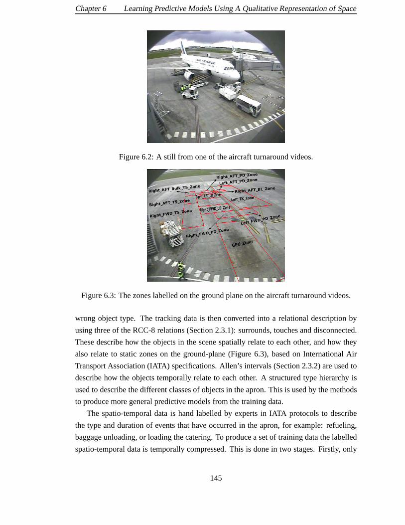
Chapter 6 Learning Predictive Models Using A Qualitative Representation of Space
Figure 6.2: A still from one of the aircraft turnaround videos.
Figure 6.3: The zones labelled on the ground plane on the aircraft turnaround videos.
wrong object type. The tracking data is then converted into arelational description by
using three of the RCC-8 relations (Section 2.3.1): surrounds, touches and disconnected.
These describe how the objects in the scene spatially relateto each other, and how they
also relate to static zones on the ground-plane (Figure 6.3), based on International Air
Transport Association (IATA) specifications. Allen’s intervals (Section 2.3.2) are used to
describe how the objects temporally relate to each other. A structured type hierarchy is
used to describe the different classes of objects in the apron. This is used by the methods
to produce more general predictive models from the trainingdata.
The spatio-temporal data is hand labelled by experts in IATAprotocols to describe
the type and duration of events that have occurred in the apron, for example: refueling,
baggage unloading, or loading the catering. To produce a setof training data the labelled
spatio-temporal data is temporally compressed. This is done in two stages. Firstly, only
145

Chapter 6 Learning Predictive Models Using A Qualitative Representation of Space
spatio-temporal data labelled with an event is kept, and non-labelled spatio-temporal data
is removed. Secondly, for each labelled event only the spatio-temporal data occurring in a
fixed length temporal window placed the end of the event is kept. Section 6.4.3.2 performs
an experiment with STGP to see how the length of the window affects the results. Each
event has a large amount of variation due to the noise in the tracking data. The training
data set contains 70 events.
6.3.1.3 Tic Tac Toe
Tic Tac Toe is a game played by two people on a 3 by 3 grid. One person uses the symbol
nought (O) and the other person uses the symbol cross (X). Each person takes it in turn
to add one of their symbols to the grid. The first person to create a line of three of their
symbols either diagonally, vertically or horizontally wins the game. The Tic Tac Toe
data was obtained from the UCI Machine Learning Repository2. The data contained a
representation of the grid for every possible end game, along with the label describing if
the person using crosses won the game.
The original data was represented in a fixed length vector, with each element of the
vector describing the symbol used at a particular location in the grid. The data was con-
verted into a relational description. Instead of representing the state of every location in
the grid only the symbols used in the grid were described along with the spatial relations
between them. Figure 6.4 shows the four spatial relations that can exist between symbols
on the grid: above, above right, above left and right. The dataset contained 800 possible
end games, and was noise free.
6.3.2 Representation
6.3.2.1 STGP
A similar representation described in Section 5.5.2.1 is used for all datasets in this chapter.
The CCTV with spatial relations dataset used only one entitydefinition which describes
the detection. There are also relation definitions for the four orientation relations. The
aircraft turnaround dataset has entity definitions for the people, and each of the possible
vehicles that can appear on the apron. There are also relation definitions for the three
RCC-8 spatial relations. The Tic Tac Toe dataset has an entity definition for the symbols
used on the grid. This has a property which describes the typeof the symbol. It also has
relation definitions for the four spatial relations shown inFigure 6.4.
2http://archive.ics.uci.edu/ml/datasets/Tic-Tac-Toe+Endgame
146

Chapter 6 Learning Predictive Models Using A Qualitative Representation of Space
Right
AboveAbove left Above right
Figure 6.4: The four spatial relations used in the Tic Tac Toedataset: above, right, aboveright, and above left.
All the datasets make use of theRelationExists function to allow the condition
section to access relations in the history; and the logical functions:And,Or andNot. The
aircraft turnaround and CCTV datasets have functions representing the Allen’s intervals,
and temporal state relations described in Chapter 5. Finally, the Tic Tac Toe dataset uses
theGet, Equal, andNot-Equal functions to allow the condition section to access and
compare the types of different symbols. The dataset also uses the terminals:Cross and
Nought.
In both Chapters 4 and 5 the action section of each productionrule used a static entity
instance, which did not use any variables from the conditionsection. In this chapter the
CCTV dataset requires that the location of the predicted detector is not at a fixed location,
but is spatially related to the location of a previous detection. The action section of the
production rules therefore needs to contain a relation rather than a static entity instance.
The relation contains a variable relating to the previous detector found in the condition
section. This illustrates the generalisation ability of the representation.
6.3.2.2 Progol, C4.5, Neural Networks, and Bayesian Networks
The same Progol representation used in Section 5.5.2.2 is used for all datasets in this
chapter. The only difference is to add the spatial relationsdescribed in Section 6.3.1 along
with the temporal relations. Again, the WEKA machine learning system and the same
representation described in Section 5.5.2.3 is used to perform the C4.5, Neural Networks,
and Bayesian Network learning algorithms. For the datasetsin this chapter the binary
feature vector not only represents every possible permutation of temporal relations, but
spatial relations as well. The approach from Chapter 4 (Section 4.9.3.1) is used to convert
147

Chapter 6 Learning Predictive Models Using A Qualitative Representation of Space
the clauses learnt by Progol into a SLP.
6.4 Results
This section will firstly show the results of an experiment tosee how robust to spatial noise
STGP using spatial relations is. Secondly it will show how STGP compares with C4.5,
Bayesian Networks, Neural Networks, and Progol on the datasets described previously.
It will also explain if estimating the likelihood of the clauses learnt by Progol, using Pe
and STGP, improves the results. Finally, the results with experimenting with some of the
different parameters for STGP is given. All the experimentsused 10 fold cross validation,
and the same evaluation criteria from Chapter 4 were used (Section 4.10.1).
6.4.1 Spatial noise robustness of STGP
An experiment was performed to see if the predictive models using spatial relations were
robust to spatial noise. The predictive models learnt from the real world CCTV dataset
in this chapter, were compared against the predictive models learnt on the same dataset
from Chapter 4. Two test sets were used: a handcrafted clean data set, and the similar
handcrafted dataset where the locations of two of the detectors were swapped. Figure 6.5
shows the results of the experiment. It can be seen that the predictive models that relied
on the detectors occurring in the specific 2D locations were affected when the location
of these detectors was changed. The predictive models that used spatial relations were
unaffected by the change in detector locations. This is because the predictive models
that rely on the detectors being in the specific locations assume the detectors will always
occur in a specific sequence. When the location of the detectors is changed, the order of
the detectors in the sequence is also changed. This preventsthe predictive model from
matching the sequence and from making a prediction. The predictive models that use
spatial relations look at the spatial change between the location the current detection, and
the previous detection. This produces a sequence based on relative spatial change between
detectors, rather than the identifiers of the detectors themselves. This will be unaffected
by the changes in the actual location of the detectors, whichis why the predictive models
using spatial relations is still be able to correctly produce a prediction.
6.4.2 A comparison of STGP with current methods
The accuracy results for the different methods on the CCTV dataset is shown in Figure
6.6. The graph shows that STGP produces the most accurate results when compared with
148

Chapter 6 Learning Predictive Models Using A Qualitative Representation of Space
50
55
60
65
70
75
80
85
90
95
100
No spatial relations
beforemovement
No spatial relations
aftermovement
Spatialrelationsbefore
movement
Spatialrelations
aftermovement
Ave
rage
Cov
erag
e (%
)
Detector movement test set results
50
55
60
65
70
75
80
85
90
95
100
No spatial relations
beforemovement
No spatial relations
aftermovement
Spatialrelationsbefore
movement
Spatialrelations
aftermovement
Ave
rage
Acc
urac
y (%
)
Detector movement test set results
Figure 6.5: Accuracy and coverage results showing how the movement in the locationof the detectors in the CCTV dataset affects the predictive models using and not usingspatial relations. The error bars show one standard deviation from the mean. All resultswere produced by 10 fold cross validation.
the other methods, and the difference in accuracy is statistically significant. The optimal
result for the CCTV dataset was 100% coverage and 83% accuracy. This is based on the
four possible actions on the path occurring in equal proportions. The results for STGP
show that it achieved less than this for both coverage and accuracy. The coverage was
reduced because STGP did not learn infrequent changes between detectors. The accuracy
was reduced because the condition sections of the production rules were not complex
enough. Most condition sections only looked at the relations between two previous detec-
tions which meant they did not predict well on the more complex patterns that involve the
relations between three or more detectors. This is because two or more production rules
would match the complex pattern and both produce a prediction reducing the overall ac-
curacy. If a production rule was learnt that could match the complex pattern only it would
produce a prediction and the accuracy would be increased.
Some of the clauses learnt by Progol were incorrect because they predict by using
data in the future. Figure 6.7 shows one of the clauses learntby Progol. It can be seen
that theeast_next, and thenorth_next clauses base their prediction on thefuture
east or north relations. There is no way to easily prevent Progol from using future
data when learning the clauses, which makes it an unsuitablemethod to learn predictive
models of temporal data. The rest of the clauses learnt were too general and made a
prediction based on whether a detection had just occurred. This can be seen in Figure 6.7
where thewest_next andsouth_next clauses just contain theenter literal. When
the likelihood of the clauses was estimated by Pe there was noimprovement in their
accuracy. This was because the over general clauses always produce a prediction, which
affects the accuracy of clauses that predict correctly. There was, however, an improvement
149

Chapter 6 Learning Predictive Models Using A Qualitative Representation of Space
in the accuracy of the results when the conflict resolver in STGP was used to estimate the
likelihood of the clauses. This is because Pe must fire all enabled production rules, and the
likelihood of a prediction is based on the likelihood of the other predictions. Incorrectly
fired production rules will reduce the accuracy of the correct predictions. The conflict
resolver in STGP can probabilistically decide based on a setof enabled production rules,
which production rules to fire which is why it gets better accuracy results than Progol
and Pe. C4.5, Neural Networks, and Bayesian Networks did notachieve high accuracy.
This is because, as explained in Chapter 5, these methods cannot generalise, and rely on
memorising frequently occurring events. If there is not enough training data to learn the
possible events, then the methods will perform poorly on thetest data, which can be seen
in the results.
0
20
40
60
80
100
Bayes Net.C4.5 NN Progol Progol+ Pe
Progol+ STGP
STGP
Mea
n C
over
age
(%)
Method
CCTV Spatial
0
20
40
60
80
100
Bayes Net.C4.5 NN Progol Progol+ Pe
Progol+ STGP
STGP
Mea
n A
ccur
acy
(%)
Method
CCTV Spatial
Figure 6.6: The accuracy and coverage results for the different methods on the CCTVSpatial dataset. The error bars show one standard deviationfrom the mean. All resultswere produced by 10 fold cross validation.
action(east_next,A,B) :- enter(A,B), east(C,A,D).action(west_next,A,B) :- enter(A,B).action(north_next,A,B) :- enter(A,B), north(C,A,D).action(south_next,A,B) :- enter(A,B).
Figure 6.7: An incorrect set of clauses learnt by Progol fromthe CCTV Spatial dataset.
The accuracy and coverage results for the different methodson the aircraft turnaround
dataset is shown in Figure 6.8. The optimal result would be 100% accuracy and 100%
coverage, and random chance would on average receive an accuracy of 6% (as there are 16
possible events). The graph shows that the results from the different methods have similar
accuracy, and the accuracy for all methods is very low (beingbelow 40% for all methods).
Neural Networks did not produce a result as WEKA failed with aStack size error when
150

Chapter 6 Learning Predictive Models Using A Qualitative Representation of Space
learning from the training data. This indicates the set of possible relations given to WEKA
was too large. The confusion matrices for STGP, Progol, Bayesian Networks and C4.5
are shown in Tables 6.2 to 6.5. Figure 6.1 provides a key to relate event numbers to
event labels. The graphs show that overall STGP achieved thelargest number of correct
predictions with a total of 14; C4.5 achieved 11 correct predictions; Bayesian Networks
achieved 6 correct predictions and Progol achieved 5.
Some of the events, like catering and loading/unloading from the plane, occur in-
frequently in the training data which explains why in all methods they are not learnt
correctly. STGP produces good coverage results when predicting aircraft arrival, but pre-
dicts less well for handler deposits chocks, and the loadingand unloading events on the
aircraft. Around a third of the time STGP is unable to producea prediction due to the
poor tracking data. Progol typically predicted Ground Power Unit (GPU) positioning for
all events, causing it to get poor results. This is due to Progol firstly not learning very
specific clauses for the events, and secondly the ordering ofthe clauses causes Progol to
always predict the same event. Bayesian Networks achieved some correct predictions for
the aircraft loading and unloading events, but gets confused between aircraft arrival and
aircraft departure. Finally, C4.5 achieved some correct predictions for Handler Deposits
Chocks and Passenger Boarding Bridge positioning, but failed to correctly predict aircraft
arrival and departure. It achieved some good results for aircraft loading events but often
confuses unloading events for loading events and vice versa.
0
20
40
60
80
100
Bayes Net. C4.5 Progol Progol+ Pe
Progol+ STGP
STGP
Mea
n C
over
age
(%)
Method
Co-FRIEND
0
20
40
60
80
100
Bayes Net. C4.5 Progol Progol+ Pe
Progol+ STGP
STGP
Mea
n A
ccur
acy
(%)
Method
Co-FRIEND
Figure 6.8: The accuracy and coverage results for the different methods on the aircraftturnaround dataset. The error bars show one standard deviation from the mean. All resultswere produced by 10 fold cross validation.
The coverage and accuracy results for the methods on the Tic Tac Toe dataset is shown
in Figure 6.9. The optimal obtainable result is 100% coverage, and 100% accuracy. The
results show that all methods except Bayesian Networks got good accuracy, and coverage
results that were close to the optimal result. STGP got mean accuracy results that were
151

Chapter 6 Learning Predictive Models Using A Qualitative Representation of Space
0=Aircraft Arrival 1=Aircraft Departure2=Catering 3=Handler Deposits Chocks4=Passenger Boarding Bridge Positioning 5=Passenger Boarding Bridge Removing6=Suitcase Loading 7=Suitcase Unloading8=Ground Power Unit Positioning 9=Ground Power Unit Removing10=Left Refuelling Operation 11=Push Back Positioning12=Right Aft Container Loading Operation 13=Right Aft Container Unloading Operation14=Right Forward Container Loading Operation 15=Right Forward Container Unloading16=No Prediction Operation
Table 6.1: The key for the event types used in the aircraft turnaround dataset.
Actual Pred.Pred. 0 1 2 3 4 5 6 7 8 9 10 11 12 13 14 15 16 Total
0 4 0 1 1 2 0 0 0 2 0 0 0 0 0 0 0 0 101 0 0 0 0 0 0 0 0 0 0 0 0 0 0 0 0 0 02 0 0 0 0 0 0 0 0 0 0 0 0 0 0 0 0 0 03 1 0 0 2 2 0 0 0 0 0 0 0 1 0 0 0 0 64 0 1 0 0 0 0 1 0 0 0 0 0 0 0 0 0 0 25 0 0 0 0 0 1 1 1 0 0 0 0 0 0 0 0 0 36 0 0 0 0 0 1 2 1 0 0 1 0 1 0 0 0 0 67 0 0 0 0 0 2 1 1 0 0 0 2 0 0 0 0 0 68 0 0 0 1 0 0 0 0 3 0 0 0 0 0 1 1 0 69 0 0 0 0 0 0 0 0 0 0 0 0 0 0 0 0 0 010 0 0 0 0 0 0 0 0 0 0 0 0 0 0 0 0 0 011 0 0 0 0 0 0 0 1 0 0 0 1 0 0 0 0 0 212 0 0 0 0 0 0 0 0 0 0 0 0 0 0 0 0 0 013 0 0 0 0 0 0 0 0 0 0 0 0 0 0 0 0 0 014 0 0 0 0 0 0 0 0 0 0 0 0 0 0 0 0 0 015 0 0 0 0 0 0 0 0 0 0 0 0 0 0 0 0 0 016 2 5 1 3 3 2 1 2 2 1 1 3 1 1 1 0 0 29
Actual 7 6 2 7 7 6 6 6 7 1 2 6 3 1 2 1 0Total
Table 6.2: The confusion matrix for STGP on the aircraft turnaround dataset.
Actual Pred.Pred. 0 1 2 3 4 5 6 7 8 9 10 11 12 13 14 15 16 Total
0 0 0 0 0 0 0 0 0 0 0 0 0 0 1 0 0 0 11 1 0 0 0 1 0 0 0 0 0 0 0 0 0 0 0 0 22 0 0 0 0 0 0 0 0 0 0 0 0 0 0 0 0 0 03 0 0 0 0 0 1 0 0 0 0 0 1 2 0 0 0 0 44 0 0 0 0 0 0 0 0 0 0 0 0 0 0 0 0 0 05 1 0 0 1 1 0 2 1 1 0 0 0 0 0 0 0 0 76 0 1 0 1 0 1 0 0 1 0 0 1 1 0 1 0 0 77 0 0 0 0 0 0 0 0 0 0 0 0 0 0 0 0 0 08 5 5 2 5 5 4 4 5 5 1 2 4 0 0 1 1 0 499 0 0 0 0 0 0 0 0 0 0 0 0 0 0 0 0 0 010 0 0 0 0 0 0 0 0 0 0 0 0 0 0 0 0 0 011 0 0 0 0 0 0 0 0 0 0 0 0 0 0 0 0 0 012 0 0 0 0 0 0 0 0 0 0 0 0 0 0 0 0 0 013 0 0 0 0 0 0 0 0 0 0 0 0 0 0 0 0 0 014 0 0 0 0 0 0 0 0 0 0 0 0 0 0 0 0 0 015 0 0 0 0 0 0 0 0 0 0 0 0 0 0 0 0 0 016 0 0 0 0 0 0 0 0 0 0 0 0 0 0 0 0 0 0
Actual 7 6 2 7 7 6 6 6 7 1 2 6 3 1 2 1 0Total
Table 6.3: The confusion matrix for Progol on the aircraft turnaround dataset.
slightly worse than Progol, C4.5 and Neural Networks. This was because STGP learnt
production rules that in some cases are not specific enough tocover all the different types
of end games. Progol got good results on the dataset because this is the type of data that
Progol has been designed to learn from (non-deterministic,and containing structural rela-
tions). A large amount of training data was used (800 out of a possible 900 games), which
152

Chapter 6 Learning Predictive Models Using A Qualitative Representation of Space
Actual Pred.Pred. 0 1 2 3 4 5 6 7 8 9 10 11 12 13 14 15 16 Total
0 1 0 0 2 1 0 0 0 2 0 1 0 0 0 0 0 0 71 3 0 0 1 3 0 1 3 1 0 1 1 0 0 0 0 0 142 0 0 0 0 0 0 0 0 0 0 0 0 0 0 0 0 0 03 1 1 0 0 0 2 1 0 0 1 0 3 2 1 0 0 0 124 0 0 0 1 0 1 0 0 0 0 0 1 0 0 0 0 0 35 2 2 1 3 1 0 0 1 3 0 0 0 0 0 1 0 0 146 0 0 1 0 1 1 3 0 0 0 0 0 1 0 0 0 0 77 0 0 0 0 0 0 1 2 0 0 0 0 0 0 1 1 0 58 0 0 0 0 0 0 0 0 0 0 0 0 0 0 0 0 0 09 0 0 0 0 0 0 0 0 0 0 0 0 0 0 0 0 0 010 0 0 0 0 0 0 0 0 0 0 0 0 0 0 0 0 0 011 0 2 0 0 1 1 0 0 0 0 0 0 0 0 0 0 0 412 0 1 0 0 0 1 0 0 1 0 0 1 0 0 0 0 0 413 0 0 0 0 0 0 0 0 0 0 0 0 0 0 0 0 0 014 0 0 0 0 0 0 0 0 0 0 0 0 0 0 0 0 0 015 0 0 0 0 0 0 0 0 0 0 0 0 0 0 0 0 0 016 0 0 0 0 0 0 0 0 0 0 0 0 0 0 0 0 0 0
Actual 7 6 2 7 7 6 6 6 7 1 2 6 3 1 2 1 0Total
Table 6.4: The confusion matrix for Bayesian Networks on theaircraft turnaround dataset.
Actual Pred.Pred. 0 1 2 3 4 5 6 7 8 9 10 11 12 13 14 15 16 Total
0 0 1 0 0 0 0 0 0 1 0 0 0 0 0 0 0 0 21 1 1 0 1 1 1 0 0 1 0 0 1 0 0 0 0 0 72 0 0 0 1 0 0 0 0 1 0 0 0 0 0 0 0 0 23 2 0 0 3 1 0 0 0 1 0 1 0 0 0 0 0 0 84 1 1 1 0 2 3 0 1 0 0 0 1 2 1 0 0 0 135 1 1 0 2 0 0 0 0 1 0 0 1 0 0 0 0 0 66 0 0 1 0 1 0 3 2 0 0 1 0 1 0 0 1 0 107 0 1 0 0 0 0 2 1 1 0 0 2 0 0 0 0 0 78 2 0 0 0 2 0 0 1 1 1 0 0 0 0 1 0 0 89 0 0 0 0 0 0 0 0 0 0 0 0 0 0 0 0 0 010 0 0 0 0 0 0 1 0 0 0 0 1 0 0 0 0 0 211 0 0 0 0 0 2 0 1 0 0 0 0 0 0 0 0 0 312 0 1 0 0 0 0 0 0 0 0 0 0 0 0 1 0 0 213 0 0 0 0 0 0 0 0 0 0 0 0 0 0 0 0 0 014 0 0 0 0 0 0 0 0 0 0 0 0 0 0 0 0 0 015 0 0 0 0 0 0 0 0 0 0 0 0 0 0 0 0 0 016 0 0 0 0 0 0 0 0 0 0 0 0 0 0 0 0 0 0
Actual 7 6 2 7 7 6 6 6 7 1 2 6 3 1 2 1 0Total
Table 6.5: The confusion matrix for C4.5 on the aircraft turnaround dataset.
meant that Neural Networks, and C4.5 had enough training data to memorise common ex-
amples. This explains why it achieved such good accuracy, and coverage results on the
test fold. When the likelihood of the clauses were estimatedby using the conflict resolver
in STGP, and Pe there was no significant change in the accuracyor coverage results.
6.4.3 Parameter experimentation with STGP
In a similar manner to Chapter 5 the STGP experiments in this chapter used the best set-
tings from Section 4.10.3. STGP has an inefficient implementation of theFind Best
Substitution algorithm (Figure 3.12). To see if a production rule matchesa set
of history, all possible combinations of objects, and theirrelations from the history that
might match its condition section are evaluated until one isfound that causes the condition
section to evaluate true. In the Tic Tac Toe, and CoFriend datasets there can be a large
number of combinations to evaluate, which has a large impacton the run-time of STGP
(a run for example might take 7 days to complete). To make the runs complete in a more
153

Chapter 6 Learning Predictive Models Using A Qualitative Representation of Space
0
20
40
60
80
100
Bayes Net.C4.5 NN Progol Progol+ Pe
Progol+ STGP
STGP
Mea
n C
over
age
(%)
Method
Tic-Tac-Toe
0
20
40
60
80
100
Bayes Net.C4.5 NN Progol Progol+ Pe
Progol+ STGP
STGP
Mea
n A
ccur
acy
(%)
Method
Tic-Tac-Toe
Figure 6.9: The accuracy results for the different methods on the Tic Tac Toe dataset. Theerror bars show one standard deviation from the mean. All results were produced by 10fold cross validation.
reasonable time a set of constraints were added to STGP. A limit on the number of com-
binations that could be searched over was added to theFind Best Substitution
algorithm. Any condition section that requires more than this number of combinations is
assumed to have evaluated false on the history. All the runs for the Tic Tac Toe dataset
also had a reduced population size of 3000, and the maximum number of generations was
reduced to 70. A potential solution to this problem is discussed in the Conclusion section
at the end of this chapter. The remainder of this section willshow experiments with two
STGP parameters: Tarpeian value, and History length to see how their values affect the
predictive models learnt by STGP.
6.4.3.1 Tarpeian value
An experiment was performed which varied the Tarpeian valuefor the Tarpeian bloat
control method [22] on the three training datasets from thischapter. The results are shown
in Figure 6.10. For the CCTV Spatial dataset there was littlechange in the accuracy
by increasing the Tarpeian value when compared to no bloat control. However for all
Tarpeian values the size of the predictive models is significantly reduced when compared
with the size of the predictive models produced with no bloatcontrol. A Tarpeian value of
4 was the optimal value. Similar results are found for the CoFriend dataset. Again there
is little change in the accuracy of the results when using bloat control when compared
to not using bloat control. For Tarpeian values below 7 thereis a statistical significant
reduction in the size of the predictive models when comparedto not using bloat control.
For the CoFriend dataset a Tarpeian value of 6 was the optimalvalue. Finally, for the Tic
Tac Toe dataset there is no statistical significant difference in both the size and accuracy
of the predictive models when using bloat control compared to not using bloat control.
154

Chapter 6 Learning Predictive Models Using A Qualitative Representation of Space
This shows that the limit on the number of combinations affects the size of the production
rules produced, and explains why using Tarpeian value control does not reduce the size
of the predictive models any further.
64
66
68
70
72
74
76
78
80
82
1098765432None
Mea
n A
ccur
acy
(%)
Tarpeian Value Full
CCTV Spatial
0
20
40
60
80
100
120
140
160
1098765432None
Mea
n S
ize
Tarpeian Value Full
CCTV Spatial
-10
-5
0
5
10
15
20
25
30
35
1098765432None
Mea
n A
ccur
acy
(%)
Tarpeian Value Full
CoFriend
-100
-50
0
50
100
150
1098765432None
Mea
n S
ize
Tarpeian Value Full
CoFriend
65
70
75
80
85
90
95
1098765432None
Mea
n A
ccur
acy
(%)
Tarpeian Value Full
TicTacToe
50
100
150
200
250
300
350
400
1098765432None
Mea
n S
ize
Tarpeian Value Full
TicTacToe
Figure 6.10: The mean accuracy and size results for the datasets on different Tarpeianvalues. The error bars show one standard deviation from the mean. All results wereproduced by 10 fold cross validation.
6.4.3.2 History length
An experiment was performed to see how the length of the history used for the CoFriend,
and CCTV Spatial datasets affected the results. For the CCTVSpatial dataset history of
155

Chapter 6 Learning Predictive Models Using A Qualitative Representation of Space
lengths 2 - 10 was used, and for the CoFriend dataset history lengths of: 5, 10, 15, 20,
25, and 30 was used. A longer history length is used for CoFriend, because the temporal
length of some of its events is much longer than the events in CCTV Spatial. Figure
6.11 shows the results from the experiments. The CCTV Spatial dataset had no change in
the accuracy of the results as the history length was increased. There was a statistically
significant decrease in the coverage of the results (p-valuebetween history length 3 to 9 is
0.002). This is because the longer history length produces more complex patterns to learn
from, which are harder for STGP to learn predictive models of. For the CoFriend dataset
there was no change in the accuracy or coverage of the resultsfor all history values.
62
64
66
68
70
72
74
76
78
80
82
2 4 6 8 10
Mea
n A
ccur
acy
(%)
History Length
CCTV Spatial
70
75
80
85
90
95
100
105
2 4 6 8 10
Mea
n C
over
age
(%)
History Length
CCTV Spatial
-5
0
5
10
15
20
25
30
35
40
0 5 10 15 20 25 30
Mea
n A
ccur
acy
(%)
History Length
CoFriend
-5
0
5
10
15
20
25
30
35
40
0 5 10 15 20 25 30
Mea
n C
over
age
(%)
History Length
CoFriend
Figure 6.11: The mean coverage and accuracy results for the CCTV Spatial, and aircraftturnaround datasets on different history length values. The error bars show one standarddeviation from the mean. All results were produced by 10 foldcross validation.
6.5 Conclusions
This chapter has shown that the use of qualitative spatial relations allows the predictive
models to be robust to spatial noise. Section 6.4.1 verified this experimentally by show-
ing that the predictive models learnt from the CCTV data in Chapter 4 (which rely on the
156

Chapter 6 Learning Predictive Models Using A Qualitative Representation of Space
detectors occurring in a specific ordering) fail when the detectors are moved. The pre-
dictive models learnt in this chapter are robust to this noise, because they use qualitative
spatial relations that look at the spatial change between the location of detections, rather
than relying on the detectors occurring in absolute locations. The accuracy results for all
methods on the CoFriend dataset was very poor. STGP got the most accurate results on
the CCTV Spatial, but got worse accuracy results than Progol, C4.5 and Neural Networks
on the Tic Tac Toe dataset. Progol, C4.5 and Neural Networks did not get very accurate
results on the CCTV Spatial dataset, but got very accurate results on the Tic Tac Toe
dataset.
STGP has an inefficient method to evaluate the condition section of a production rule
on a history. It was shown to be an issue (Section 6.4.3) on theCoFriend, and Tic Tac Toe
datasets, as large combinations of entities and relations need to be checked. Techniques
from databases, or Prolog could be used to fix this problem. These would match parts of
the condition section to parts of the history, until an overall match is found. This makes
it a more efficient search process than looking over all possible combinations from the
history that might match the condition section.
Progol has no temporal constraints during its search to find the most general clause.
This can cause it to predict using relations or entities fromthe future, as was shown in
the results from the CCTV Spatial dataset. One way to preventthis from happening is to
only allow Progol to see previous spatio-temporal data whenit is generalising the most
specific clause. This would require changing how the most specific clause is generated,
to take into account temporal constraints from the data.
157

Chapter 7
Automatic Bloat Control in Genetic
Programming
7.1 Introduction
In Chapters 4 - 6 experiments were performed using STGP to seewhat was the best
Tarpeian value for different datasets. The experiments hadtwo main conclusions. Firstly,
there was no universal optimal Tarpeian value for all datasets. Datasets which require
a simpler predictive model typically have a lower optimal Tarpeian value, than datasets
which require more complex predictive models. Secondly, having a fixed Tarpeian value
may not produce the most accurate and smallest predictive models.
Ekart and Nemeth [21] adapt the diversity of the population during the run. In the
initial stages of the run a high diversity is maintained, andin the later stages of the run a
lower diversity is allowed to force GP to converge on a solution. This chapter investigates
a similar technique to vary the Tarpeian value during the runof STGP. It is proposed that
during a run a high Tarpeian value (causing high population diversity) is typically required
at the start to help STGP find good solutions, and a lower Tarpeian value (causing lower
population diversity) is then required once STGP has converged on a solution to reduce
the size of the predictive models. This chapter investigates using an adaptive Tarpeian
method that varies the Tarpeian value during the run based onthe current and initial best
fitness values. Section 7.2 presents the method, and Section7.3 shows the results of the
158

Chapter 7 Automatic Bloat Control in Genetic Programming
method applied to the datasets from Chapters 4 - 6.
7.2 Adaptive Tarpeian value
The results from Chapters 4 - 6 showed that there was not a single Tarpeian value that
will guarantee both good coverage, and accuracy, and small sized predictive models for
all datasets. The problem is that some datasets like Uno and Uno2 require a low Tarpeian
value from the start to get a good solution. However, others like PSS, and Uno Temporal
need a higher Tarpeian value to get accurate predictive models, but it is not small enough
in the later stages of the run to produce very small predictive models.
The Tarpean bloat control method can be seen as controlling the size of the population.
Low Tarpeian values will greatly reduce the size of the population that is sampled from
by the genetic operators, and this creates a lower population diversity. Lower diversity
allows STGP to find small solutions once it has a correct solution, but can prevent STGP
from initially finding a correct solution. High Tarpeian values allow a larger population
size to be sampled from by the genetic operators, which leadsto a higher diversity. This is
good for allowing a more comprehensive initial search of thesearch space, but can make
it hard for STGP to focus on a small correct solution later on in the runs. This chapter
proposes (based on the work of [21]) that a high diversity is required at the start of the run
to allow a good set of predictive models to be evolved, and lowdiversity at the end of the
run to find compact predictive models.
There has been previous work (Section 2.6.7) in GP on adaptive diversity [21], and
adaptive population size [110]. Ekart and Nemeth [21] usea gradient based technique
that looks at the ratio of the current and previous best fitness values to adapt their diversity
controls. Rochatet al. [110] use an absolute method that looks at the ratio of the current
best fitness and the initial best fitness to adapt the population size. The same approach has
been taken in this chapter to adapt the Tarpeian value. The approach assumes that how
close the current best fitness value is to the optimal fitness value (0), relates to how much
Tarpeian bloat control should be applied. When the current best fitness value is a long
way from the optimal fitness value a high Tarpeian value should be used to allow STGP
to investigate a range of possible solutions. However, whenthe current best fitness value
is close to the optimal value a low Tarpeian value can be used to force STGP to converge
on a small correct solution. Equation 7.1 shows the method toautomatically adapt the
Tarpeian value. The new Tarpeian valuet is defined as the ratio of the current best fitness
fb to the initial best fitnessfi multiplied by the initial Tarpeian valuetinitial . In all the
experiments the initial Tarpeian value is set to 10. To prevent the Tarpeian value from
159

Chapter 7 Automatic Bloat Control in Genetic Programming
going to 1 (which would cause all the predictive models that were above the average size
to be removed from the population) it is limited to a minimum value of 2. This method
was applied to the datasets from Chapters 4 - 6. The results are shown in the next section.
t = Max(fcfi∗ tinitial ,2) (7.1)
7.3 Results
Figures 7.1 - 7.11 show the results for the adaptive Tarpeianmethod on the datasets from
Chapters 4 - 6. The results show that the adaptive Tarpeian method got accuracy results on
all the noisy datasets, and most of the clean datasets that were as good as the best results
using a fixed Tarpeian value. It also typically produced predictive models of a size equal
to or smaller than the most accurate predictive models usinga fixed Tarpeian value.
The results on the PSS datasets (Figure 7.1) show that the method does not get very
accurate results for the clean dataset. It is too aggressive, causing it to produce small sized
predictive models, with accuracy results that are worse than the most accurate results from
using a fixed Tarpeian value. The noise results on the Uno2 datasets (Figure 7.3) show that
as the level of noise is increased the method produces predictive models that are larger on
average than most accurate predictive models produced using a fixed Tarpeian value. The
results on the CCTV datasets (Figure 7.4) show that the accuracy of the method on the
clean dataset is lower than the best accuracy using the fixed Tarpeian value. The results
on the PYCR datasets (Figure 7.5) are similar to the ones for CCTV. On the clean, and
10% noise datasets it gets the smallest size results, but theaccuracy results are worse than
the best accuracy results using a fixed Tarpeian value. The CCTV dataset using spatial
relations (Figure 7.6) gets a similar accuracy result to using a fixed Tarpeian value, but
the average size of the predictive model is larger than the best results from using a fixed
Tarpeian value.
The results have highlighted two main issues with the method. Firstly, the method
assumes that a very small current best fitness (less than 0.10) means that STGP is very
close to finding the correct solution, and consequently a high level of bloat control can be
used to reduce the size of the predictive model. However, forthe clean PSS and PYCR
datasets a very low fitness value does not always mean that STGP is close to finding
the correct solution. When the adaptive Tarpeian method is applied to these datasets it
incorrectly decreases the Tarpeian value causing a decrease in the diversity of the popu-
lation causing STGP to prematurely converge on an incomplete solution. Secondly, on
the noisy datasets, the noise limits the minimum value for the current best fitness that a
160

Chapter 7 Automatic Bloat Control in Genetic Programming
predictive model can achieve. This affects the smallest possible Tarpeian value that the
adaptive Tarpeian method can produce. In the later stages ofthe runs the amount of bloat
control is reduced which prevents STGP from finding the smallest possible models. This
can be seen, for example, in the results for the Uno2 datasets, and the CCTV with spatial
relations dataset.
7.4 Conclusions
The previous chapters has shown that there is no universal fixed Tarpeian value that will
work well on all datasets. This chapter has shown an adaptiveTarpeian method which
computes the Tarpeian value based on the ratio of the currentbest fitness to the initial best
fitness. The results showed that the method got accuracy results that were as good as the
best results using a fixed Tarpeian method, for all the noisy datasets, and most of the clean
datasets. There are two main problems with the method. Firstly, it reduces the Tarpeian
value too quickly for some of the clean datasets, causing STGP to prematurely converge
on an incomplete solution. Secondly, the noise in the datasets affects the method making
it unable to produce low Tarpeian values. To solve these problems some form of scaling
could be used to convert the ratio between the current best fitness and the initial best
fitness into a Tarpeian value. An exponential scale could be used for the clean datasets to
allow high Tarpeian values to be still used when the current best fitness has a low value.
On the noisy datasets a constant noise value (based on the noise level) could be removed
from the ratio to allow it to produce low Tarpeian values.
161
Chapter 7 Automatic Bloat Control in Genetic Programming
88
90
92
94
96
98
100
102
104
1098765432Auto
Mea
n A
ccur
acy
(%)
Tarpeian Value
PSS - Clean
10
20
30
40
50
60
70
80
90
1098765432Auto
Mea
n S
ize
Tarpeian Value
PSS - Clean
78
80
82
84
86
88
90
92
94
1098765432Auto
Mea
n A
ccur
acy
(%)
Tarpeian Value
PSS - 10% Noise
0
50
100
150
200
250
300
1098765432Auto
Mea
n S
ize
Tarpeian Value
PSS - 10% Noise
60
62
64
66
68
70
72
74
76
1098765432Auto
Mea
n A
ccur
acy
(%)
Tarpeian Value
PSS - 30% Noise
0
50
100
150
200
250
300
350
1098765432Auto
Mea
n S
ize
Tarpeian Value
PSS - 30% Noise
Figure 7.1: The accuracy and size results for the Auto Tarpeian method on the PSS dataset.The error bars show one standard deviation from the mean. Allresults were produced by10 fold cross validation.
162

Chapter 7 Automatic Bloat Control in Genetic Programming
98.4
98.6
98.8
99
99.2
99.4
99.6
99.8
100
100.2
100.4
1098765432Auto
Mea
n A
ccur
acy
(%)
Tarpeian Value
Uno - Clean
15
20
25
30
35
40
45
1098765432Auto
Mea
n S
ize
Tarpeian Value
Uno - Clean
82
84
86
88
90
92
94
96
1098765432Auto
Mea
n A
ccur
acy
(%)
Tarpeian Value
Uno - 10% Noise
0
50
100
150
200
250
1098765432Auto
Mea
n S
ize
Tarpeian Value
Uno - 10% Noise
54
56
58
60
62
64
66
68
70
72
1098765432Auto
Mea
n A
ccur
acy
(%)
Tarpeian Value
Uno - 30% Noise
0
50
100
150
200
250
300
350
1098765432Auto
Mea
n S
ize
Tarpeian Value
Uno - 30% Noise
Figure 7.2: The accuracy and size results for the Auto Tarpeian method on the Unodatasets. The error bars show one standard deviation from the mean. All results wereproduced by 10 fold cross validation.
163

Chapter 7 Automatic Bloat Control in Genetic Programming
84
86
88
90
92
94
96
98
100
102
1098765432Auto
Mea
n A
ccur
acy
(%)
Tarpeian Value
Uno2 - Clean
10
15
20
25
30
35
40
45
50
1098765432Auto
Mea
n S
ize
Tarpeian Value
Uno2 - Clean
60
65
70
75
80
85
90
1098765432Auto
Mea
n A
ccur
acy
(%)
Tarpeian Value
Uno2 - 10% Noise
0
20
40
60
80
100
120
140
160
1098765432Auto
Mea
n S
ize
Tarpeian Value
Uno2 - 10% Noise
40
45
50
55
60
65
1098765432Auto
Mea
n A
ccur
acy
(%)
Tarpeian Value
Uno2 - 30% Noise
0
20
40
60
80
100
120
140
160
180
200
220
1098765432Auto
Mea
n S
ize
Tarpeian Value
Uno2 - 30% Noise
Figure 7.3: The accuracy and size results for the Auto Tarpeian method on the Uno2datasets. The error bars show one standard deviation from the mean. All results wereproduced by 10 fold cross validation.
164

Chapter 7 Automatic Bloat Control in Genetic Programming
74
76
78
80
82
84
86
88
90
1098765432Auto
Mea
n A
ccur
acy
(%)
Tarpeian Value
CCTV - Clean
0
20
40
60
80
100
120
140
160
180
200
1098765432Auto
Mea
n S
ize
Tarpeian Value
CCTV - Clean
68
70
72
74
76
78
80
82
84
1098765432Auto
Mea
n A
ccur
acy
(%)
Tarpeian Value
CCTV - 10% Noise
0
20
40
60
80
100
120
140
160
180
200
1098765432Auto
Mea
n S
ize
Tarpeian Value
CCTV - 10% Noise
54
56
58
60
62
64
66
68
70
72
74
1098765432Auto
Mea
n A
ccur
acy
(%)
Tarpeian Value
CCTV - 30% Noise
0
20
40
60
80
100
120
140
160
180
1098765432Auto
Mea
n S
ize
Tarpeian Value
CCTV - 30% Noise
Figure 7.4: The accuracy and size results for the Auto Tarpeian method on the CCTVdatasets. The error bars show one standard deviation from the mean. All results wereproduced by 10 fold cross validation.
165

Chapter 7 Automatic Bloat Control in Genetic Programming
82
84
86
88
90
92
94
1098765432Auto
Mea
n A
ccur
acy
(%)
Tarpeian Value
PYCR - Clean
0
50
100
150
200
250
300
1098765432Auto
Mea
n S
ize
Tarpeian Value
PYCR - Clean
68
70
72
74
76
78
80
82
84
1098765432Auto
Mea
n A
ccur
acy
(%)
Tarpeian Value
PYCR - 10% Noise
0
50
100
150
200
250
300
350
400
1098765432Auto
Mea
n S
ize
Tarpeian Value
PYCR - 10% Noise
50
52
54
56
58
60
62
64
66
68
70
1098765432Auto
Mea
n A
ccur
acy
(%)
Tarpeian Value
PYCR - 30% Noise
0
50
100
150
200
250
300
1098765432Auto
Mea
n S
ize
Tarpeian Value
PYCR - 30% Noise
Figure 7.5: The accuracy and size results for the Auto Tarpeian method on the PYCRdatasets. The error bars show one standard deviation from the mean. All results wereproduced by 10 fold cross validation.
166

Chapter 7 Automatic Bloat Control in Genetic Programming
60
65
70
75
80
85
1098765432Auto
Mea
n A
ccur
acy
(%)
Tarpeian Value
CCTV Temporal (Clean)
0
20
40
60
80
100
120
140
1098765432Auto
Mea
n S
ize
Tarpeian Value
CCTV Temporal (Clean)
55
60
65
70
75
80
1098765432Auto
Mea
n A
ccur
acy
(%)
Tarpeian Value
CCTV Temporal (Real World)
0
20
40
60
80
100
120
140
1098765432Auto
Mea
n S
ize
Tarpeian Value
CCTV Temporal (Real World)
64
66
68
70
72
74
76
78
80
82
1098765432Auto
Mea
n A
ccur
acy
(%)
Tarpeian Value
CCTV Spatial
0
10
20
30
40
50
60
70
80
90
100
1098765432Auto
Mea
n S
ize
Tarpeian Value
CCTV Spatial
Figure 7.6: The accuracy and size results for the Auto Tarpeian method on the CCTVdataset using temporal relations, and the CCTV dataset using spatial relations. The errorbars show one standard deviation from the mean. All results were produced by 10 foldcross validation.
167

Chapter 7 Automatic Bloat Control in Genetic Programming
88
90
92
94
96
98
100
1098765432Auto
Mea
n A
ccur
acy
(%)
Tarpeian Value
Uno Temporal
0
20
40
60
80
100
120
140
160
180
1098765432AutoM
ean
Siz
eTarpeian Value
Uno Temporal
82
84
86
88
90
92
94
96
1098765432Auto
Mea
n A
ccur
acy
(%)
Tarpeian Value
Uno Temporal with Noise
0
50
100
150
200
250
300
1098765432Auto
Mea
n S
ize
Tarpeian Value
Uno Temporal with Noise
Figure 7.7: The accuracy and size results for Auto Tarpeian method on the Uno Temporaldatasets. The error bars show one standard deviation from the mean. All results wereproduced by 10 fold cross validation.
168
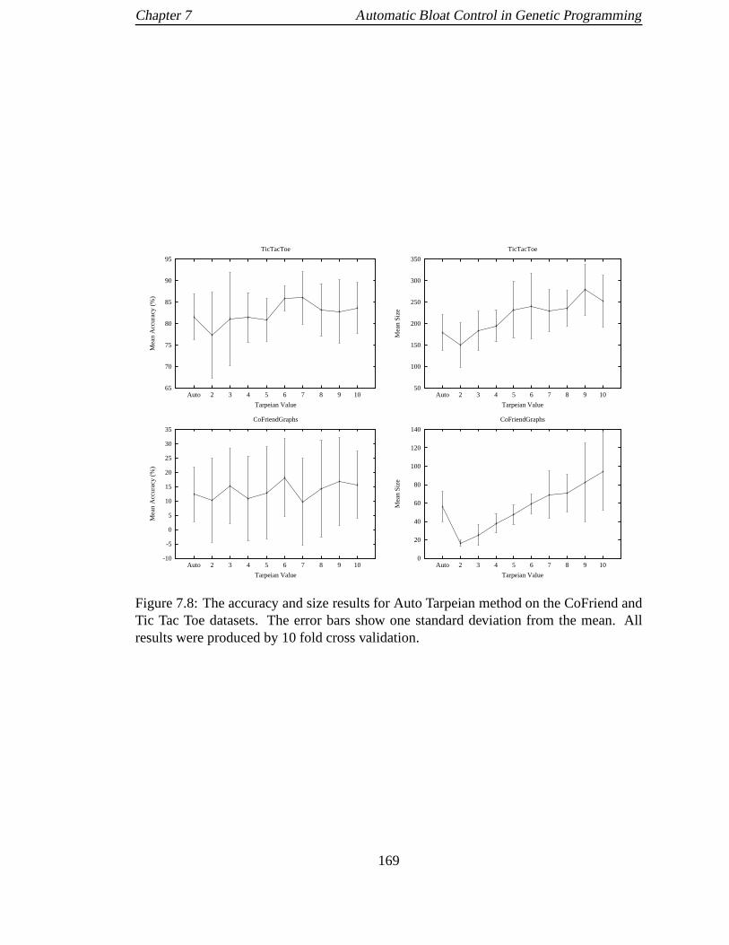
Chapter 7 Automatic Bloat Control in Genetic Programming
65
70
75
80
85
90
95
1098765432Auto
Mea
n A
ccur
acy
(%)
Tarpeian Value
TicTacToe
50
100
150
200
250
300
350
1098765432AutoM
ean
Siz
eTarpeian Value
TicTacToe
-10
-5
0
5
10
15
20
25
30
35
1098765432Auto
Mea
n A
ccur
acy
(%)
Tarpeian Value
CoFriendGraphs
0
20
40
60
80
100
120
140
1098765432Auto
Mea
n S
ize
Tarpeian Value
CoFriendGraphs
Figure 7.8: The accuracy and size results for Auto Tarpeian method on the CoFriend andTic Tac Toe datasets. The error bars show one standard deviation from the mean. Allresults were produced by 10 fold cross validation.
169

Chapter 7 Automatic Bloat Control in Genetic Programming
78
80
82
84
86
88
90
1098765432Auto
Mea
n A
ccur
acy
(%)
Tarpeian Value
PSS - Clean
-5
0
5
10
15
20
25
30
35
40
45
50
1098765432Auto
Mea
n S
ize
Tarpeian Value
PSS - Clean
74
76
78
80
82
84
86
1098765432Auto
Mea
n A
ccur
acy
(%)
Tarpeian Value
PSS - 10% Noise
2
4
6
8
10
12
14
16
18
20
22
1098765432Auto
Mea
n S
ize
Tarpeian Value
PSS - 10% Noise
56
58
60
62
64
66
68
70
72
74
76
78
1098765432Auto
Mea
n A
ccur
acy
(%)
Tarpeian Value
PSS - 30% Noise
0
10
20
30
40
50
60
70
80
1098765432Auto
Mea
n S
ize
Tarpeian Value
PSS - 30% Noise
Figure 7.9: The accuracy and size results for the Auto Tarpeian method on the PSS dataset,where the predictive models are using a simple conflict resolver. The error bars show onestandard deviation from the mean. All results were producedby 10 fold cross validation.
170

Chapter 7 Automatic Bloat Control in Genetic Programming
80
82
84
86
88
90
92
94
1098765432Auto
Mea
n A
ccur
acy
(%)
Tarpeian Value
Uno - Clean
-5
0
5
10
15
20
25
30
35
40
1098765432Auto
Mea
n S
ize
Tarpeian Value
Uno - Clean
72
74
76
78
80
82
84
86
88
90
92
1098765432Auto
Mea
n A
ccur
acy
(%)
Tarpeian Value
Uno - 10% Noise
-10
0
10
20
30
40
50
60
70
1098765432Auto
Mea
n S
ize
Tarpeian Value
Uno - 10% Noise
50
55
60
65
70
75
80
1098765432Auto
Mea
n A
ccur
acy
(%)
Tarpeian Value
Uno - 30% Noise
-10
0
10
20
30
40
50
60
70
80
90
100
1098765432Auto
Mea
n S
ize
Tarpeian Value
Uno - 30% Noise
Figure 7.10: The accuracy and size results for the Auto Tarpeian method on the Unodatasets, where the predictive models are using a simple conflict resolver. The error barsshow one standard deviation from the mean. All results were produced by 10 fold crossvalidation.
171
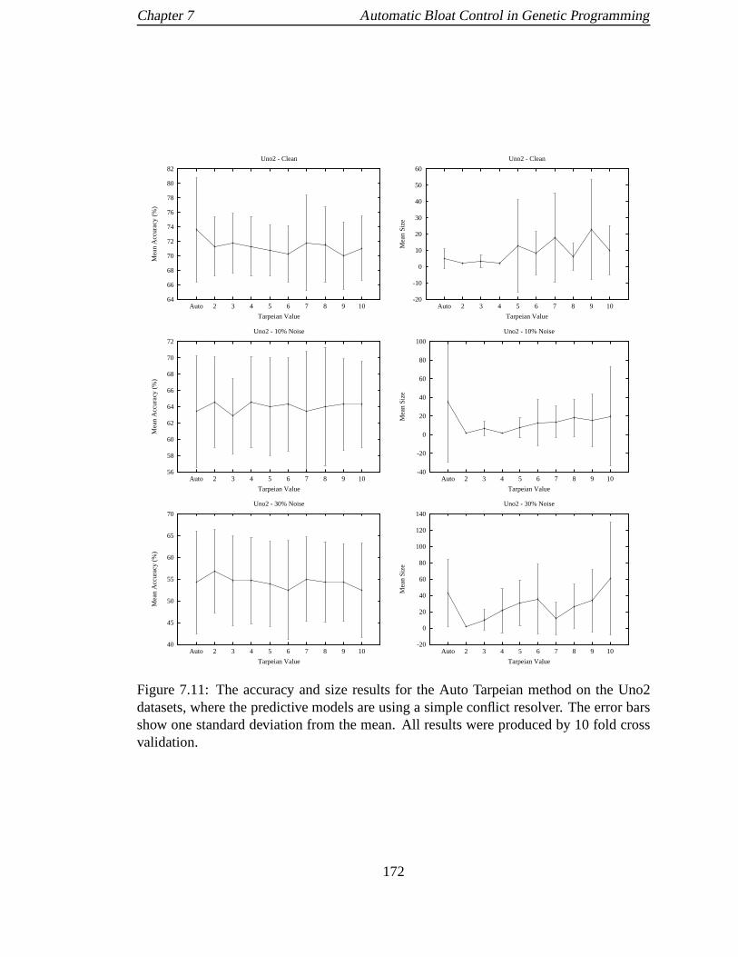
Chapter 7 Automatic Bloat Control in Genetic Programming
64
66
68
70
72
74
76
78
80
82
1098765432Auto
Mea
n A
ccur
acy
(%)
Tarpeian Value
Uno2 - Clean
-20
-10
0
10
20
30
40
50
60
1098765432Auto
Mea
n S
ize
Tarpeian Value
Uno2 - Clean
56
58
60
62
64
66
68
70
72
1098765432Auto
Mea
n A
ccur
acy
(%)
Tarpeian Value
Uno2 - 10% Noise
-40
-20
0
20
40
60
80
100
1098765432Auto
Mea
n S
ize
Tarpeian Value
Uno2 - 10% Noise
40
45
50
55
60
65
70
1098765432Auto
Mea
n A
ccur
acy
(%)
Tarpeian Value
Uno2 - 30% Noise
-20
0
20
40
60
80
100
120
140
1098765432Auto
Mea
n S
ize
Tarpeian Value
Uno2 - 30% Noise
Figure 7.11: The accuracy and size results for the Auto Tarpeian method on the Uno2datasets, where the predictive models are using a simple conflict resolver. The error barsshow one standard deviation from the mean. All results were produced by 10 fold crossvalidation.
172

Chapter 8
Conclusions
8.1 Summary of the work
This thesis has shown a technique to learn predictive modelsfrom spatio-temporal data.
In Chapter 3 a frame based [78] representation for the spatio-temporal history data
was described. The representation enables a set of entities, and relationships between the
entities to be described. Relations and entities can also have properties which can also
be represented. Each different type of property, entity or relation requires a definition,
which is represented by a class frame. This definition is usedto create property, entity
or relation instances, which are represented by instance frames. A predictive model is
represented by a production system, which contains a set of production rules, and conflict
resolver. The production rules describe different possible patterns in the history and their
possible future outcomes: Each production rule typically models different parts of the
activity being modelled. Production rules contain two sections: a condition section that
matches a specific subset of the history; and an action section that represents a new entity
or relation. The conflict resolver is a conditional probability distribution represented as a
Bayesian Network. It takes as its input a set of enabled production rules, and computes the
likelihood that a subset of these production rules will be fired to produce a prediction. The
chapter concluded by explaining an inference technique which given a predictive model,
and a history will produce a prediction.
Chapter 4 described how a predictive model is learnt from thespatio-temporal history
173

Chapter 8 Conclusions
data using Spatio-Temporal Genetic Programming (STGP). The chapter described how
the predictive models were initially generated, the fitnessfunction, and the genetic oper-
ators used. It also explained how the parameters of the conflict resolver are computed.
A bloat control technique is used (the Tarpeian method [22])to control the size of the
predictive models. Five datasets were used to evaluate the system. Four were based on
the card games: Uno, Papers Scissors Stone and Play your cards right; and one based on
people walking along a path.
The method presented in this thesis (STGP) achieved the mostaccurate results on all
the datasets in this chapter in comparison to a set of existing machine learning methods:
Progol, Neural Networks, Bayesian Networks, C4.5 and Pe. Progol managed to learn the
correct clauses for many of the datasets, but it was unable toapply them in the correct
order, which affected both its coverage and accuracy results. When Progol was combined
with Pe (a technique to estimate the probability of the clauses when used as a stochastic
logic program) it managed to improve Progol’s coverage, butdue to clashing clauses it
did not often improve its accuracy. Pe must fire all enabled production rules, and the
likelihood of a prediction is based on the likelihood of the other predictions. Sometimes
an enabled production rule will produce an incorrect prediction when it is fired, which
affects Pe’s accuracy. The conflict resolver used by STGP canprobabilistically decide
which of the enabled production rules to fire. This prevents enabled production rules that
produce incorrect predictions from being fired. It was shownthat when the clauses learnt
by Progol were estimated by the conflict resolver in STGP it improved both their coverage,
and accuracy results. Bayesian Networks and C4.5 performedfairly well on the datasets
in this chapter, but were limited due to their inability to learn generalised rules from the
data. It was shown that STGP produces the best results with: some form of size control on
the predictive models; the tournament selection sampling technique using a tournament
selection value that favours the better scoring predictivemodels; and an increased amount
of adding and replacement of production rules in the initial10 generations of the run.
Chapter 5 showed the use of qualitative temporal relations in the predictive models. A
novel temporal state relation to relate the time range of an entity or relation instance to the
current time was presented. Handcrafted Uno datasets; and real-world and handcrafted
CCTV datasets were used for the experiments. Again, STGP produced the most accurate
predictive models for all datasets. Progol did not manage tolearn clauses complex enough
to correctly predict from the training data. Estimating thelikelihood of the clauses using
Pe did not improve the accuracy of the results. When the likelihood of the clauses were
estimated by STGP the coverage, and accuracy of the results were improved except for the
noise free CCTV dataset. Again, the inability for Neural Networks, Bayesian Networks,
174
Chapter 8 Conclusions
and C4.5 to generalise from data affected the accuracy of their results. It was shown
experimentally that using temporal relations in the predictive models when compared to
not using them allowed STGP to be robust to injection noise, and to be slightly more
accurate when predicting from scenes containing multiple people. Finally, it was shown
that increasing history length used by the predictive models reduced their coverage and
accuracy results.
Chapter 6 demonstrated the use of spatio-temporal relations in the condition section of
the production rules, and the ability to use relations in theaction section of the production
rules. The temporal relations were the same as the ones used in Chapter 5. The chapter
verified experimentally that predictive models that use spatial relations between objects
are robust to spatial noise when compared to predictive models that do not use spatial
relations. Three datasets were used for the experiments: CCTV, aircraft turnarounds, and
Tic Tac Toe. STGP was shown to have an inefficient technique toevaluate the condition
section of the production rules on the history, which had a large impact on its run-time on
the Tic Tac Toe and aircraft turnaround datasets. Section 8.4 explains a possible solution
to this problem. Progol learnt overly general clauses on theCCTV datasets, and sometime
the clauses it learnt based their predictions on relations occurring in the future. There is
no easy way to prevent this from happening, which makes Progol unsuitable for learning
from temporal data.
Chapter 7 firstly described an adaptive Tarpeian method which computes the Tarpeian
value based on the ratio of the current best fitness to the initial best fitness. The method
was evaluated using all the datasets from the previous chapters. The results showed that
the method got accuracy results that were as good as the best results using a fixed Tarpeian
method, for all the noisy datasets, and most of the clean datasets. The results showed two
main problems with the method. Firstly, it reduces the Tarpeian value too quickly for some
of the clean datasets, causing STGP to prematurely convergeon an incomplete solution.
Secondly, the noise in the datasets affects the method making it unable to produce low
Tarpeian values. Section 8.4 explains possible solutions to these problems.
8.2 Contributions
The main contributions from this thesis are:
1. A novel predictive model architecture represented as a production system. Each
production rule models a separate part of the spatio-temporal data. The conflict
resolver (represented as a Bayesian Network) allows the architecture to model non-
deterministic data, and to use a set of production rules to make a prediction.
175

Chapter 8 Conclusions
2. A novel temporal relation that relates the time range of anentity or relation instance
in the history to the current prediction time.
3. A technique to learn predictive models by Genetic Programming.
4. The use of spatial relations within the condition sectionof the production rule.
5. Initial work on a technique to adapt the Tarpean bloat value during the run of STGP.
8.3 Discussion
Chapter 1 introduced six questions that this thesis has attempted to investigate. This
section will show to what extent this thesis has managed to answer them.
Question 1: Does representing the components of the predictive models using first or-
der logic, produce more accurate results on non-deterministic spatio-temporal data
than using standard machine learning representations?
In Chapters 4 - 6 experiments were performed on two techniques using first order logic:
STGP, and Progol; along with three techniques using standard machine learning represen-
tations: Neural Networks, Bayesian Networks, and C4.5. Theresults showed that STGP,
and Progol produced more generalised results than Neural Networks, Bayesian Networks,
or C4.5. These can not generalise in many situations and effectively rely on storing com-
mon examples and their outcomes. The accuracy results for STGP and Progol (when
combined with STGP) were shown to be as good as or better than the accuracy results for
Neural Networks, Bayesian Networks and C4.5.
Question 2: Does using a probabilistic conflict resolver produce more accurate pre-
dictive models on non-deterministic spatio-temporal datathan other conflict resolu-
tion approaches?
The results from the datasets in Chapters 4 - 6 showed that thesimple conflict resolver
used by Progol did not produce such good coverage and accuracy results as the probabilis-
tic conflict resolvers used by STGP, and Pe. The clauses learnt by Progol are evaluated in
the default manner used in Prolog. This applies the clauses in order until one entails the
unseen example. If the clauses are placed in the wrong order Progol will predict incor-
rectly and the accuracy of its results will be affected (Section 4.10.2). These results can
be improved by using Pe and STGP. On all datasets Pe improved the coverage results of
176
Chapter 8 Conclusions
Progol, but did not always improve its accuracy results. This is because Pe must fire all
enabled production rules, and the likelihood of a prediction is based on the likelihood of
the other predictions. Incorrectly fired production rules will reduce the accuracy of the
correct predictions. The probabilistic conflict resolver presented in this thesis can decide,
based on a set of enabled production rules, which productionrules to fire. This in some
cases, significantly improves the accuracy results when compared against the accuracy
results from Progol and Pe.
Question 3: Does using evolutionary search techniques to learn production rules
produce more accurate results on non-deterministic spatio-temporal data than using
a deterministic (greedy) search?
STGP uses a genetic programming based approach to learn the production rules. It was
shown that for all datasets (except Tic Tac Toe) that STGP produced predictive models
which had an accuracy that was the same as, or better than the accuracy for all other
methods. Progol is an alternative technique to learn the production rules. It uses a
greedy search, but did not get accuracy results (even when combined with the proba-
bilistic conflict resolver presented in this thesis) that were better than STGP. The results
on the datasets from Chapters 5 and 6 were often too general, and it shows that Progol did
not fully search for good clauses.
Question 4: Does learning the production rules and the parameters of the conflict
resolver simultaneously produce more accurate results on non-deterministic spatio-
temporal data than learning them sequentially?
The results from Chapters 4 - 6 showed that (apart for Tic Tac Toe) STGP was as accurate
or more accurate than all other methods. This shows that the combined approach to learn-
ing the production rules and the conflict resolver parameters used by STGP was more
accurate than the sequential approach of using Progol to learn the production rules, and
then using Pe or STGP to estimate the parameters for the conflict resolver. The combined
approach allows the learner to use the properties of the conflict resolver as part of the
predictive model learning process. This allows the learnerto allow different production
rules to be enabled at the same time to produce simpler and smaller predictive models as
shown in Section 3.3.
177

Chapter 8 Conclusions
Question 5: Does use of qualitative temporal relations within the components of
the predictive models make them robust to changes in the temporal structure of the
non-deterministic spatio-temporal data?
Section 5.6.1 presented the results of an experiment where predictive models using tem-
poral relations and predictive models not using temporal relations were tested on datasets
containing injection noise, and multiple people. Overall the predictive models using tem-
poral relations were not affected, by the injection noise; and were more accurate when
predicting from the dataset containing multiple people than the predictive models not us-
ing temporal relations. This shows that using temporal relations in the predictive models
makes them robust to some changes in the temporal structure of the spatio-temporal data.
Question 6: Does use of qualitative spatial relations within the components of the
predictive models make them robust to changes in the spatialstructure of the non-
deterministic spatio-temporal data?
Section 6.4.1 showed results of an experiment where predictive models using, and not
using qualitative spatial orientation relations were firstly tested on a clean dataset, and
secondly on a dataset where the location of some of the objects was changed. The pre-
dictive models that used spatial relations were unaffectedby the change in the location of
the objects, but the predictive models that did not use spatial relations were affected by
this change. This shows that spatial relations are robust tosome changes in the spatial
structure of the spatio-temporal data. Further work could be done using different spatial
relations, and different test datasets containing different forms of spatial noise. The spatial
noise could take the form of different types of camera movement like horizontal, vertical,
or zooming. It could also take the form of occlusion where parts of the image are hidden.
8.4 Future work
This thesis has highlighted a variety of problems that are potential avenues of future work:
1. Methods could be investigated for improving the speed of STGP in finding a solu-
tion and improving the accuracy of the solution. A simplistic method is currently
used to vary the type, and probability of genetic operators used during the run. This
only allows the genetic operators that operate on the predictive model for the initial
n generations, and then uses genetic operators that operate on both the predictive
model and the production rules for the rest of the run. Another approach is to adapt
178

Chapter 8 Conclusions
the operator type, and probabilities during the run. This idea been successfully ap-
plied in the context of GP [91]. Using these techniques within STGP would allow
it to use the optimal set of operators during the different stages of the run. This
should allow STGP to find more accurate solutions in a reducedamount of genera-
tions. This is an easy project and could be done as an undergraduate dissertation.
2. Chapter 7 described a method to automatically adjust the Tarpeian value based on
the ratio of the current best fitness to the initial best fitness. The results showed
that it did not work for all datasets. The method was affectedby noise in the data,
and can often reduce the Tarpeian value too quickly on clean datasets. To fix these
problems the ratio between the current best fitness and the initial best fitness could
be applied to a scaling function to convert it into a Tarpeianvalue. Work could be
performed to see which scaling functions produced the best results on the clean,
and noisy datasets. This is an easy project and could be done as an undergraduate
dissertation.
3. Currently the condition section of a production rule is created randomly. However,
Progol initialises its search for the most general clause bygenerating and using the
most specific clause. This is then used to bound the search. Allowing the condition
section to be some variant on the most specific clause could reduce the search space,
and make finding a solution faster. This is a harder project and could be done as a
masters thesis.
4. It was assumed in this thesis that all the predictions madeby the predictive models
were for the next time step. In noisy datasets it may not always be the case that
the current prediction will happen at the next time step. Forexample with multiple
people in a scene the system might predict that a person will perform a particular
action, but before it happens a different person might have already performed an
action. Techniques could be investigated that allow STGP totake a series of predic-
tions from a predictive model and decide when each prediction should be applied.
This could be used to more accurately predict when future actions might occur. This
is a hard project and could be done as a PhD thesis.
5. In all the datasets used in this thesis the entities, relations and their properties have
a probability of 1. In the real world the probability of entities, relations and their
properties can be less than 1, representing uncertainty in information received the
world. For example, a tracking algorithm might use a probability less than 1 for
the type of an object when it is unsure of the type it could be classified as. There
179

Chapter 8 Conclusions
has been previous work to learn models based on first order logic where the data is
uncertain, for example Markov Logic Networks [106], Stochastic Logic Programs
[18], and Bayesian Logic Programs [53]. The ideas from this research could be
incorporated into STGP to allow it to learn and predict from uncertain data. This is
also a harder project and could be done as a masters thesis.
6. Chapter 6 showed how relations could be used in the action section of the produc-
tion rule. The relations could use variables from the condition section to represent
entities. Section 3.3.1.2 showed in theory how the properties of entities from the
history could be used in the action section. This has not beenimplemented, or
experimented on in this thesis. Further work could be done toimplement and ex-
periment with this. This would create more generalised production rules, which
should help STGP to find a solution faster. It would also allowthe predictive mod-
els to contain less production rules. This is a harder project and could be done as a
masters thesis.
7. Work could be done to apply STGP to more complex domains that have a larger
number of objects, and more complex behaviour patterns to learn. This is an open
problem and might require a team of researchers to work on it.
8. Work could be done to investigate extra genetic operatorsthat could be used in
STGP. This would allow it to find solutions faster, and to better investigate the
search space. This is a harder project and could be done as a masters thesis.
9. Chapter 6 highlighted problems with the algorithm to see if the condition section
of a production rule was enabled on some history. It was shownto be inefficient
when there are large numbers of combinations of relations and entities in the history
to check against. Work could be done to investigate alternative algorithms. One
potential approach could be to use a Prolog or database search style approach where
instead of matching the whole tree against the history sub-trees are matched on the
history in turn until an overall match is found. This is an easy project and could be
done as an undergraduate dissertation.
180

Bibliography
[1] J. F. Allen. Maintaining knowledge about temporal intervals. Communications of
the ACM, 26:198–3, 1983.
[2] P. J. Angeline and J. Pollack. Evolutionary module acquisition. In Proceedings
of the Second Annual Conference on Evolutionary Programming, pages 154–163.
MIT Press, 1993.
[3] C. Anglano, A. Giordana, G. Lo Bello, and L. Saitta. An experimental evaluation of
coevolutive concept learning. InProceedings of the 15th International Conference
on Machine Learning, pages 19–27, 1998.
[4] S. Augier, G. Venturini, and Y. Kodratoff. Learning firstorder logic rules with a
genetic algorithm. InProcedings of the 1st International Conference on Knowledge
Discovery and Data Mining, pages 21–26, 1995.
[5] J. E. Baker. Adaptive selection methods for genetic algorithms. InProceedings of
the First International Conference on Genetic Algorithms and Their Applications,
pages 101–111, 1985.
[6] J. E. Baker. Reducing bias and inefficiency in the selection algorithm. InProceed-
ings of the Second International Conference on Genetic Algorithms, pages 14–21,
1987.
[7] A. Baumberg and D. Hogg. An efficient method for contour tracking using active
shape models. InProceedings of the IEEE Workshop on Motion of Non-Rigid and
Articulated Objects, pages 194–199, 1994.
[8] D. Beymer, P. McLauchlan, B. Coifman, and J. Malik. A real-time computer vision
system for measuring traffic parameters. InProceedings of IEEE Conference on
Computer Vision and Pattern Recognition, pages 495–501, 1997.
181

BIBLIOGRAPHY
[9] M. Biba, S. Ferilli, and F. Esposito. Structured learning of Markov logic networks
through iterated local search. InProceedings of the European Conference on Artif-
ical Intelligence, pages 361–366, 2008.
[10] T. Bray, J. Paoli, C. M. Sperberg-McQueen, E. Maler, andF. Yergeau. eXtensi-
ble Markup Language (XML) 1.0 (Fourth Edition). W3C recommendation, W3C,
2006. http://www.w3.org/TR/2006/REC-xml-20060816/.
[11] C. Bregler. Learning and recognising human dynamics invideo sequences. In
Proceedings of the IEEE Computer Society Conference on Computer Vision and
Pattern Recognition, pages 568–574, 1997.
[12] E. K. Burke, S. Gustafson, and G. Kendall. Diversity in genetic programming: An
analysis of measures and correlation with fitness.IEEE Transactions on Evolution-
ary Computation, 8:47–62, 2004.
[13] A. G. Cohn and S. M Hazarika. Qualitative spatial representation and reasoning:
An overview.Fundamenta Informaticae, 46(1-2):1–29, 2001.
[14] S. Colton. An application-based comparison of automated theory formation and
inductive logic programming.Electronic Transactions on Artificial Intelligence,
4:97–117, 2000.
[15] S. Colton and S. Muggleton. Mathematical applicationsof inductive logic pro-
gramming.Machine Learning, 64:25–64, 2006.
[16] G. F. Cooper and E. Herskovits. A Bayesian method for theinduction of proba-
bilistic networks from data.Machine Learning, 9:309–347, 1992.
[17] G. Csurka, C. Dance, L. Fan, J. Willamowski, and C. Bray.Visual categorization
with bags of keypoints. InProceedings of the Workshop on Statistical Learning in
Computer Vision at European Conference on Computer Vision, pages 1–22, 2004.
[18] J. Cussens. Parameter estimation in stochastic logic programs.Machine Learning,
44:245–271, 2001.
[19] J. Davis, E. Burnside, I. de Castro Dutra, D. Page, and V.Santos Costa. An in-
tergrated approach to learning Bayesian networks of rules.In Proceedings of the
Sixteenth European Conference on Machine Learning, volume 3720 ofLecture
Notes in Computer Science, pages 84–95. Springer-Verlag, 2005.
182

BIBLIOGRAPHY
[20] A. Dempster, N.M. Laird, and D.B.Rubin. Maximum likelihood from incomplete
data via the EM algorithm.Journal of the Royal Statistical Society B, 39:1–39,
1977.
[21] A. Ekart and S. Z. Nemeth. Maintaining the diversity of genetic programs. In
Proceedings of the European Conference on Genetic Programming, volume 2278
of Lecture Notes in Computer Science, pages 162–171. Springer-Verlag, 2002.
[22] A. Ekart and S. Z. Nemeth. A simple but theoretically-motivated method to control
bloat in genetic programming. InProceedings of the 6th European Conference on
Genetic Programming, volume 2610 ofLecture Notes in Computer Science, pages
211–223. Springer-Verlag, 2003.
[23] D. Federico. Evolutionary concept learning in first order logic: An overview.AI
Communications, 19(1):13–33, 2006.
[24] L. Fei-Fei and P. Perona. A Bayesian hierarchical modelfor learning natural scene
categories. InProceedings of the IEEE Computer Society Conference on Computer
Vision and Pattern Recognition, pages 524–531, 2005.
[25] A. Fern and R. Givan. Sequential inference with reliable observations: Learning to
construct force-dynamic models.Artificial Intelligence, 170:1081–1100, 2006.
[26] A. P. Fern, R. L. Givan, and J. M. Siskind. Specific-to-general learning for tem-
poral events with application to learning event definitionsfrom video. Journal of
Artificial Intelligence Research (JAIR), 17:379–449, 2002.
[27] J. Fernyhough, A. G. Cohn, and D. C. Hogg. Constructing qualitative event models
automatically from video input.Image and Vision Computing, 18:81–103, 2000.
[28] J. Ferryman, S. Maybank, and A. Worrall. Visual surveillance for moving vehicles.
International Journal of Computer Vision, 37(2):187–197, 2000.
[29] P. Flach and N. Lachiche. Confirmation-guided discovery of first-order rules with
Tertius.Machine Learning, 42:61–95, 2001.
[30] P. Flach and N. Lachiche. Naive Bayesian classificationof structured data.Machine
Learning, 57:233–269, 2004.
[31] S. Forrest. Scaling fitnesses in the genetic algorithm.In Documentation for PRIS-
ONERS DILEMMA and NORMS Programs That Use the Genetic Algorithm,
1985.
183

BIBLIOGRAPHY
[32] D. A. Forsyth and J. Ponce.Computer Vision: A Modern Approach. Prentice Hall,
2003.
[33] N. Friedman, L. Getoor, D. Koller, and A. Pfeffer. Learning probabilistic relational
models. InProceedings of the Sixteenth International Conference on Artificial
Intelligence, pages 1300–1309, 1999.
[34] A. Galata, A. G. Cohn, D. Magee, and D. Hogg. Modeling interaction using learnt
qualitative spatio-temporal relations and variable length Markov models. InPro-
ceedings of the European Conference on Artificial Intelligence, pages 741–745,
2002.
[35] A. Galata, N. Johnson, and D. Hogg. Learning behaviour models of human ac-
tivities. In Proceedings of the British Machine Vision Conference, pages 12–22,
1999.
[36] A. Giordana and F. Neri. Search-intensive concept induction. Evolutionary Com-
putation, 3(4):375–416, 1996.
[37] D. E. Goldberg.Genetic Algorithms in Search, Optimization and Machine Learn-
ing. Addison-Wesley Longman Publishing Co., Inc., Boston, MA,USA, 1989.
[38] D. E. Goldberg. A note on Boltzmann tournament selection for genetic algo-
rithms and population-orientated simulated annealing.Complex Systems, 4:445–
460, 1990.
[39] K. Grauman and T. Darrell. The pyramid match kernel: Discriminative classifica-
tion with sets of image features. InProceedings of the International Conference
on Computer Vision, 2005.
[40] P. Haddawy. Generating Bayesian networks from probability logic knowledge
bases. InProceedings of the Tenth Conference on Uncertanity in Artificial In-
telligence, pages 262–269, 1994.
[41] M. Hall, E. Frank, G. Holmes, B. Pfahringer, P. Reutemann, and I. H. Witten. The
WEKA data mining software: An update.SIGKDD. E.plorations, 11(1), 2009.
[42] I. Haritaoglu, D. Harwood, and L. S. Davis.W4: Real time survellance of people
and their activities.IEEE Transactions on Pattern Analysis and Machine Intelli-
gence, 22(8):809 – 830, 2000.
184

BIBLIOGRAPHY
[43] P. E. Hart, R. O. Dura, and M. T. Einaudi. PROSPECTOR; a computer-based
consultation system for mineral exploration.Mathematical Geology, 10:589–610,
1978.
[44] D. Heckerman, D. Geiger, and D. M. Chickering. LearningBayesian networks:
The combination of knowledge and statistical data.Machine Learning, 20:197–
243, 1995.
[45] D. Hernandez. Qualitative Representation of Spatial Knowledge. Springer-
Verlang, 1994.
[46] J. Hezanaho. DOGMA: A GA-based relational learner. InProceedings of the 8th
International Conference on Inductive Logic Programming, pages 205–214, 1998.
[47] D. Hogg. Model-based vision: A program to see a walking person. Image and
Vision Computing, 1:5–20, 1983.
[48] J.H. Holland.Adaption in Natural and Artificial Systems. University of Michigan
Press, 1975.
[49] Y. Ivanov and A. Bobick. Recognition of visual activities and interactions by
stochastic parsing.IEEE Transactions On Pattern Analysis And Machine Intel-
ligence, 22(8):852–872, 2000.
[50] T. Joachims. Text categorization with support vector machines: Learning with
many relevant features. InProceedings of the European Conference on Machine
Learning, pages 137–142. Springer, 1998.
[51] R. Kalman. A new approach to linear filtering and prediction problems.Journal of
Basic Engineering, 82:35–46, 1960.
[52] W. Kantschik and W. Banzhaf. Linear-tree GP and its comparison with other GP
structures. InProceedings of the European Conference on Genetic Programming,
volume 2038 ofLecture Notes in Computer Science, pages 302–312. Springer-
Verlag, 2001.
[53] K. Kersting and L. De Raedt. Towards combining inductive logic programming
with Bayesian networks. InProceedings of the 11th International Conference on
Inductive Logic Programming, volume 2157 ofLecture Notes in Artifical Intelli-
gence, pages 118–131. Springer-Verlag, 2001.
185
BIBLIOGRAPHY
[54] V. Kettnaker and M. Brand. Minimum-entropy models of scene activity. InPro-
ceedings of the 1999 IEEE Computer Society Conference on Computer Vision and
Pattern Recognition, pages 281–286, 1999.
[55] S. Kok and P. Domingos. Learning the structure of Markovlogic networks. In
Proceedings of the 22nd International Conference on Machine Learning, pages
441–448. ACM Press, 2005.
[56] D. Koller, K. Daniilidis, and H. H. Nagel. Model based object tracking in monoc-
ular image sequences of road traffic scenes.International Journal of Computer
Vision, 37(3):257–281, 1993.
[57] D. Koller and A. Pfeffer. Probabilisitic frame-based systems. InProceedings of
the fifteenth national/tenth conference on Artificial intelligence/Innovative appli-
cations of artificial intelligence, pages 580 – 587, 1998.
[58] J. Koza.Genetic Programming. MIT Press, 1992.
[59] J. Koza.Genetic Programming II. MIT Press, 1994.
[60] J. Koza, F. H Bennett III, D. Andre, and M. Keane.Genetic Programming III.
Morgan Kaufmann, 1999.
[61] N. Landwehr, K. Kersting, and L. De Raedt. IntergratingNaıve Bayes and FOIL.
Machine Learning Research, 8:481–507, 2007.
[62] P. Larranaga, M. Poza, Y. Yurramendi, R. H. Murga, and C. M. H. Kuijpers. Struc-
ture learning of Bayesian networks by genetic algorithms: Aperformance analysis
of control parameters.IEEE Transactions on Pattern Analysis and Machine Intel-
ligence, 18(9):912–926, 1996.
[63] P. Lichodzijewski and M. Heywood. GP classifier problemdecomposition using
first-price and second-price auctions. InProceedings of the 10th European con-
ference on Genetic programming, volume 4445 ofLecture Notes in Computer Sci-
ence, pages 137–147. Springer-Verlag, 2007.
[64] T. List and R. Fisher. CVML - an XML-based computer vision markup language.
In Proceedings of the 17th International Conference on Pattern Recognition, pages
789–792, 2004.
186

BIBLIOGRAPHY
[65] E. G. Lopaz, R. Poli, and C. A. C. Coello. Reusing code ingenetic programming.
In Proceedings of the 7th European Conference on Genetic Programming, volume
3003 ofLecture Notes in Computer Science, pages 359–368, 2004.
[66] G.F. Luger.Artificial Intelligence: Structures and Strategies for Complex Problem
Solving. Addison Wesley, 2004.
[67] S. Luke and L. Panait. A comparison of bloat control methods for genetic program-
ming. Evolutionary Computation, 14(3):309–344, 2006.
[68] D. Magee. Tracking multiple vehicles using foreground, background and motion
models.Image and Vision Computing, 22:143–155, 2004.
[69] N. Maillot, M. Thonnat, and A. Boucher. Towards ontology-based cognitive vision.
Machine Vision and Applications, 16:33–40, 2004.
[70] J. McCarthy and P. J. Hayes. Some philosophical problems from the standpoint of
artifical intelligence.Machine Intelligence, 4:463–502, 1969.
[71] D. McDermott. A temporal logic for reasoning about processes and plans.Cogni-
tive Science, 6:101–155, 1982.
[72] A. Mcintyre and M. Heywood. MOGE: GP classification problem decomposition
using multi-objective optimization. InProceedings of the 8th annual conference
on Genetic and evolutionary computation, pages 863–870, 2006.
[73] A. R. McIntyre and M. I. Heywood. On multi-class classification by way of nich-
ing. In Proceedings of the Genetic and Evolutionary Computation Conference,
pages 581–592, 2004.
[74] S.J. McKenna, S. Jabri, Z. Duric, and H. Wechsler. Tracking interacting people. In
Proceedings of the Fourth IEEE International Conference onAutomatic Face and
Gesture Recognition, pages 348–353, 2000.
[75] N. Metropolis, A. Rosenbluth, M. Rosenbluth, A. Teller, and E. Teller. Equations
of state calculations by fast computing machines.Journal of Chemical Physics,
21:1087–1091, 1953.
[76] R. Michalski and J. Larson. Incremental generation of VL1 hypotheses: the un-
derlying methodology and the description of program AQ11. ISG 83-5, Computer
Science Department, Univ. of Illinois at Urbana-Champaign, 1980.
187

BIBLIOGRAPHY
[77] J. Miller and P. Thomson. Cartesian genetic programming. In Proceedings of the
European Conference on Genetic Programming, volume 1802 ofLecture Notes in
Computer Science, pages 121–132. Springer-Verlag, 2000.
[78] M. Minsky. A framework for representing knowledge.The Psychology of Com-
puter Vision, pages 211–277, 1975.
[79] D. J. Montana. Strongly typed genetic programming.Evolutionary Computation,
3:199–230, 1995.
[80] D. Moore and I. Essa. Recognizing multitasked activities from video using stochas-
tic context-free grammar. InProceedings of the Eighteenth national conference on
Artificial intelligence, pages 770–776, 2001.
[81] S. Muggleton. Learning structure and parameters of stochastic logic programs. In
Proceedings of the 12th international conference on Inductive logic programming,
volume 2583 of Lecture Notes In Artificial Intelligence, pages 198–206, 2003.
[82] S. H. Muggleton. Inverse entailment and Progol.New Generation Computing,
13:245–286, 1995.
[83] S. H. Muggleton. Stochastic logic programs. In L. de Raedt, editor,Advances in
Inductive Logic Programming, pages 254–264. IOS Press, 1996.
[84] S. H. Muggleton. Learning stochastic logic programs.Electronic Transactions in
Artificial Intelligence, 4(41), 2000.
[85] S. H. Muggleton and J. Firth. CProgol4.4: a tutorial introduction. In S. Dzeroski
and N. Lavrac, editors,Relational Data Mining, pages 160–188. Springer-Verlang,
2001.
[86] S. H. Muggleton, H. Lodhi, A. Amini, and M. J. E. Sternberg. Support vector
inductive logic programming. InProceedings of the 8th International Conference
on Discovery Science, volume 3735 of Lecture Notes in Artificial Intelligence,
pages 163–175. Springer-Verlag, 2005.
[87] S. H. Muggleton and A. Tamaddoni-Nezhad. QG/GA: A stochastic search for
Progol.Machine Learning, 70(2-3):123–133, 2007.
188

BIBLIOGRAPHY
[88] C. Needham, D. Magee, P. Santos, and S. Rao. Inducing thefocus of attention by
observing patterns in space. InProceedings of the Workshop on Modelling Oth-
ers from Observations at International Joint Conferences on Artificial Intelligence,
pages 47–52, 2005.
[89] C. Needham, P. Santos, D. Magee, V. Devin, D. Hogg, and A.G. Cohn. Protocols
from perceptual observations.Artificial Intelligence, 167:103–136, 2005.
[90] J. Niebles, H. Wang, and L. Fei-Fei. Unsupervised learning of human action cate-
gories using spatial-temporal words. InProceedings of the British Machine Vision
Conference, volume 3, pages 1249–1258, 2006.
[91] J. Niehaus and W. Banzhaf. Adaption of operator probabilities in genetic program-
ming. In Proceedings of the 4th European Conference on Genetic Programming,
volume 2038 of Lecture Notes In Computer Science, pages 325 –336, 2001.
[92] N. Oliver, B. Rosario, and A. Pentland. A Bayesian computer vision system for
modeling human interactions.IEEE Transactions on Pattern Analysis and Machine
Intelligence, 22(8):831–843, 2000.
[93] L. Panait and S. Luke. Alternative bloat control methods. In Proceedings of the
Genetic and Evolutionary Computation Conference, volume 3103 ofLecture Notes
in Computer Science, pages 630–641. Springer-Verlag, 2004.
[94] J. Pearl. Probabilistic Reasoning in Intelligent Systems: Networksof Plausible
Inference. Morgan Kaufmann, 1988.
[95] R. Poli, B. Langdon, and N. McPhee.A Field Guide To Genetic Programming.
Lulu Enterprises, UK Ltd, 2008.
[96] U. Pompe and I. Kononenko. Linear space induction in first order logic with relief.
In R. Kruse, R. Viertl and G. Della Riccia (Eds.), CISM Lecture notes, Udine Italy.
Springer Verlang, 1994.
[97] U. Pompe and I. Kononenko. Naive Bayesian classification within ILP-R. InPro-
ceedings of the Fifth International Workshop on Inductive Logic Programming,
pages 417–436, 1995.
[98] A. Puech and S. H. Muggleton. A comparison of stochasticlogic programs and
Bayesian logic programs. InProceedings of the Workshop on Learning Statisti-
cal Models from Relational Data at International Joint Conferences on Artificial
Intelligence, 2003.
189

BIBLIOGRAPHY
[99] J. Quinlan.C4.5: Programs for Machine Learning. Morgan Kaufmann, 1993.
[100] J. R. Quinlan. Learning logical definitions from relations. Machine Learning,
5:239–266, 1990.
[101] J. R. Quinlan. Boosting first-order learning. InProceedings of the 7th Interna-
tional Workshop on Algorithmic Learning Theory, volume 1160 of Lecture Notes
in Computer Science, pages 143–155, 1996.
[102] L. R. Rabiner. A tutorial on hidden Markov models and selected applications in
speech recognition.Proceedings of the IEEE, 77(2), 1989.
[103] L. De Raedt and L. Dehaspe. Clausal discovery.Machine Learning, 26:99–146,
1997.
[104] L. De Raedt and K. Kersting. Probablistic logic learning. SIGKDD. E.plorations,
2:1–17, 2003.
[105] D. A. Randell, Z. Cui, and A. G. Cohn. A spatial logic based on regions and
connection. InProceedings of the 3rd International Conference on Knowledge
Representation and Reasoning, pages 165–176, San Mateo, 1992. Morgan Kauf-
mann.
[106] M. Richardson and P. Domingos. Markov logic networks.Machine Learning,
62:107–136, 2006.
[107] J. Rissanen. Universal coding, information, prediction, and estimation. IEEE
Transactions on Information Theory, IT-30(4):629–636, 1984.
[108] S. Roberts, D. Howard, and J. Koza. Evolving modules ingenetic programming
by subtree encapsulation. InProceedings of the European Conference on Genetic
Programming, volume 2038 ofLecture Notes in Computer Science, pages 160–
175. Springer-Verlag, 2001.
[109] J. A. Robinson. A machine-oriented logic based on the resolution principle.Jour-
nal of the Assoication for Computing Machinery, 12:23–41, 1965.
[110] D. Rochat, M. Tomassini, and L. Vanneschi. Dynamic size populations in dis-
tributed genetic programming. InProceedings of the European Conference on
Genetic Programming, volume 3447 ofLecture Notes in Computer Science, pages
50–61. Springer-Verlag, 2005.
190

BIBLIOGRAPHY
[111] S. Russell and P. Norvig.Artificial Intelligence: A Modern Approach. Prentice
Hall, 2003.
[112] P. Santos, S. Colton, and D. Magee. Predictive and descriptive approaches to learn-
ing game rules from vision data. InProceedings of the Ibero-American Artificial In-
telligence Conference, volume 2709 ofLecture Notes in Computer Science, pages
349–359. Springer-Verlag, 2006.
[113] P. Santos, D. Magee, A. Cohn, and D. Hogg. Combining multiple answers for
learning mathematical structures from visual observation. In Proceedings of the
16th European Conference on Artificial Intelligence, pages 544–548, 2004.
[114] P. Santos, C. Needham, and D. Magee. Inductive learning spatial attention.Revista
Controle and Automacao, 19(3), 2008.
[115] R. Schapire. The boosting approach to machine learning: An overview. InPro-
ceedings of the MSRI Workshop on Nonlinear Estimation and Classification, 2002.
[116] E. H. Shortliffe and B. G. Buchanan. A model of inexact reasoning in medicine.
Mathematical Biosciences, 23:351–379, 1975.
[117] J. M. Siskind. Grounding the lexical semantics of verbs in visual perception using
force dynamics and event logic.Artificial Intelligence Research, 15:31–90, 2000.
[118] J. Sivic, B. Russell, A. Efros, A. Zisserman, and W. Freeman. Discovering objects
and their location in images. InProceedings of the International Conference on
Computer Vision, pages 370–377, 2005.
[119] M. Sonka, V. Hlavac, and R.D. Boyle.Image Processing, Analysis and Machine
Vision, 2nd edition. Brooks Cole, 1998.
[120] T. Soule and J. Foster. Effects of code growth and parsimony pressure on popula-
tions in genetic programming.Evolutionary Computation, 6(4):293–309, 1999.
[121] A. Srinivasan.The Aleph Manual. University of Oxford, 1999.
[122] A. Srinivasan. A study of two sampling methods for analyzing large datasets with
ILP. Data Mining and Knowledge Discovery, 3(1):95–123, 1999.
[123] T. Starner and A. Pentland. Real-time american sign language recognition from
video using hidden markov models. InProceedings of the International Symposium
on Computer Vision, pages 265–270, 1995.
191

BIBLIOGRAPHY
[124] C. Stauffer and W Grimson. Adaptive background mixture models for real-time
tracking. InProceedings of the IEEE Conference on Computer Vision and Pattern
Recognition, pages 246–252, 1999.
[125] N. Sumpter and A. Bulpitt. Learning spatio-temporal patterns for predicting object
behaviour.Image and Vision Computing, 18:697–704, 2000.
[126] A. Tamaddoni-Nezhad and S. H. Muggleton. Using genetic algorithms for learn-
ing clauses in first-order logic. InProceedings of the Genetic and Evolutionary
Computation Conference, pages 639–646. Morgan Kaufmann Publishers, 2001.
[127] V. Vapnik. The Nature of Statistical Learning Theory. Springer-Verlag, New York,
1995.
[128] M. Vilian. A system for reasoning about time. InProceedings of the AAAI, pages
197–201, 1982.
[129] F. Zelezny, A. Srinivasan, and C. D. Page Jr. Randomised restarted search in ILP.
Machine Learning, 64:183–208, 2006.
[130] D. Whitley. A genetic algorithm tutorial. Technical Report CS-93-103, Department
of Computer Science, Colorado State University, 1993.
[131] M. L. Wong and K. S. Leung. Genetic logic programming and applications.IEEE
Expert, 10(5):68–76, 1995.
[132] C. Wren, A. Azabayejani, T. Darrell, and A. Pentland. Pfinder: real-time tracking
of the human body.IEEE Transactions on Pattern Analysis and Machine Intelli-
gence, 19(7):780–785, 1997.
[133] L. Q. Xu and D. C. Hogg. Neural networks in human motion tracking - An exper-
imental study.Image and Vision Computing, 15:607–615, 1997.
192