using elasticities to derive optimal bankruptcy exemptions · using elasticities to derive optimal...
TRANSCRIPT

Using Elasticities to DeriveOptimal Bankruptcy Exemptions
Eduardo Davila
NYU Stern
Structural reforms in the wake of recovery: Where do we stand?Bank of SpainJune 18 2015
Eduardo Davila (NYU Stern) Optimal Bankruptcy Exemptions 1 / 16

Motivation
Question
How large should bankruptcy exemptions be?
• Exemption: dollar amount borrower gets to keep if he does not repay
• Substantial variation on exemptions across regions/time
• This paper1. Characterizes the optimal bankruptcy exemption and dW
dm
• Very generally
2. As a function of a few measurable sufficient statistics• Calibrates optimal exemption
Eduardo Davila (NYU Stern) Optimal Bankruptcy Exemptions 2 / 16

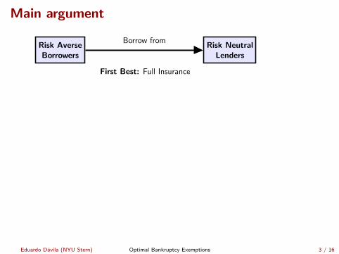
Main argument
Risk AverseBorrowers
Risk NeutralLenders
Borrow from
First Best: Full Insurance(((((((((((((hhhhhhhhhhhhhFirst Best: Full InsuranceKey Friction: Debt contract (baseline model)
Incomplete markets (extension)
Second Best: Bankruptcy exemption provides partial insurance
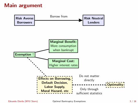
Exemption ↑
Marginal Benefit:More consumption
when bankrupt
Marginal Cost:Higher interest rates
Effects on Borrowing,Default Decision,
Labor Supply,Moral Hazard, etc
Optimality
Do not matterdirectly
Only throughsufficient statistics
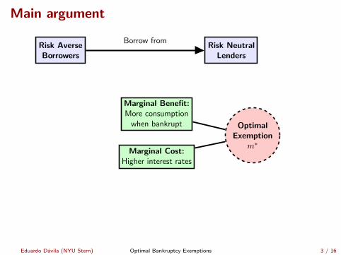
OptimalExemption
m∗
Sufficient statistic logic(CAPM analogy)
Eduardo Davila (NYU Stern) Optimal Bankruptcy Exemptions 3 / 16
Main argument
Risk AverseBorrowers
Risk NeutralLenders
Borrow from
First Best: Full Insurance
(((((((((((((hhhhhhhhhhhhhFirst Best: Full InsuranceKey Friction: Debt contract (baseline model)
Incomplete markets (extension)
Second Best: Bankruptcy exemption provides partial insurance
Exemption ↑
Marginal Benefit:More consumption
when bankrupt
Marginal Cost:Higher interest rates
Effects on Borrowing,Default Decision,
Labor Supply,Moral Hazard, etc
Optimality
Do not matterdirectly
Only throughsufficient statistics
OptimalExemption
m∗
Sufficient statistic logic(CAPM analogy)
Eduardo Davila (NYU Stern) Optimal Bankruptcy Exemptions 3 / 16

Main argument
Risk AverseBorrowers
Risk NeutralLenders
Borrow from
First Best: Full Insurance
(((((((((((((hhhhhhhhhhhhhFirst Best: Full Insurance
Key Friction: Debt contract (baseline model)Incomplete markets (extension)
Second Best: Bankruptcy exemption provides partial insurance
Exemption ↑
Marginal Benefit:More consumption
when bankrupt
Marginal Cost:Higher interest rates
Effects on Borrowing,Default Decision,
Labor Supply,Moral Hazard, etc
Optimality
Do not matterdirectly
Only throughsufficient statistics
OptimalExemption
m∗
Sufficient statistic logic(CAPM analogy)
Eduardo Davila (NYU Stern) Optimal Bankruptcy Exemptions 3 / 16

Main argument
Risk AverseBorrowers
Risk NeutralLenders
Borrow from
First Best: Full Insurance(((((((((((((hhhhhhhhhhhhhFirst Best: Full Insurance
Key Friction: Debt contract (baseline model)Incomplete markets (extension)
Second Best: Bankruptcy exemption provides partial insurance
Exemption ↑
Marginal Benefit:More consumption
when bankrupt
Marginal Cost:Higher interest rates
Effects on Borrowing,Default Decision,
Labor Supply,Moral Hazard, etc
Optimality
Do not matterdirectly
Only throughsufficient statistics
OptimalExemption
m∗
Sufficient statistic logic(CAPM analogy)
Eduardo Davila (NYU Stern) Optimal Bankruptcy Exemptions 3 / 16

Main argument
Risk AverseBorrowers
Risk NeutralLenders
Borrow from
First Best: Full Insurance(((((((((((((hhhhhhhhhhhhhFirst Best: Full InsuranceKey Friction: Debt contract (baseline model)
Incomplete markets (extension)
Second Best: Bankruptcy exemption provides partial insurance
Exemption ↑
Marginal Benefit:More consumption
when bankrupt
Marginal Cost:Higher interest rates
Effects on Borrowing,Default Decision,
Labor Supply,Moral Hazard, etc
Optimality
Do not matterdirectly
Only throughsufficient statistics
OptimalExemption
m∗
Sufficient statistic logic(CAPM analogy)
Eduardo Davila (NYU Stern) Optimal Bankruptcy Exemptions 3 / 16

Outline of the talk
1. Baseline model• Positive analysis• Welfare analysis ⇒ dW
dm and m∗ (main results)
2. Extensions
3. Calibration
4. Conclusion
Eduardo Davila (NYU Stern) Optimal Bankruptcy Exemptions 4 / 16
Environment (baseline model)• Two dates t = 0, 1
• Risk averse borrowers
maxB0
U (C0) + βE[max
U(CD1), U(CN1)]
,
C0 = y0 + q0 (B0,m)B0 CN1 = y1 −B0
CD1 = min y1,m
1. Stochastic endowment y1 (assets), cdf F (·), support on[y1, y1
]
2. Debt contract (key friction)
3. Constant bankruptcy exemption: m dollars4. Regularity conditions on F (·) and preferences5. Equilibrium: borrowers internalize q0 (B0,m)
• Risk neutral lenders
• Required return 1 + r∗, fraction δ deadweight loss in bankruptcy• Zero profit
Eduardo Davila (NYU Stern) Optimal Bankruptcy Exemptions 5 / 16

Environment (baseline model)• Two dates t = 0, 1
• Risk averse borrowers
maxB0
U (C0) + βE[max
U(CD1), U(CN1)]
,
C0 = y0 + q0 (B0,m)B0 CN1 = y1 −B0
CD1 = min y1,m
1. Stochastic endowment y1 (assets), cdf F (·), support on[y1, y1
]
2. Debt contract (key friction)3. Constant bankruptcy exemption: m dollars4. Regularity conditions on F (·) and preferences5. Equilibrium: borrowers internalize q0 (B0,m)
• Risk neutral lenders• Required return 1 + r∗, fraction δ deadweight loss in bankruptcy• Zero profit
Eduardo Davila (NYU Stern) Optimal Bankruptcy Exemptions 5 / 16

Environment (baseline model)• Two dates t = 0, 1
• Risk averse borrowers
maxB0
U (C0) + βE[max
U(CD1), U(CN1)]
,
C0 = y0 + q0 (B0,m)B0 CN1 = y1 −B0
CD1 = min y1,m
1. Stochastic endowment y1 (assets), cdf F (·), support on[y1, y1
]
2. Debt contract (key friction)
3. Constant bankruptcy exemption: m dollars4. Regularity conditions on F (·) and preferences5. Equilibrium: borrowers internalize q0 (B0,m)
• Risk neutral lenders• Required return 1 + r∗, fraction δ deadweight loss in bankruptcy• Zero profit
Eduardo Davila (NYU Stern) Optimal Bankruptcy Exemptions 5 / 16

Environment (baseline model)• Two dates t = 0, 1
• Risk averse borrowers
maxB0
U (C0) + βE[max
U(CD1), U(CN1)]
,
C0 = y0 + q0 (B0,m)B0 CN1 = y1 −B0
CD1 = min y1,m
1. Stochastic endowment y1 (assets), cdf F (·), support on[y1, y1
]
2. Debt contract (key friction)3. Constant bankruptcy exemption: m dollars
4. Regularity conditions on F (·) and preferences5. Equilibrium: borrowers internalize q0 (B0,m)
• Risk neutral lenders• Required return 1 + r∗, fraction δ deadweight loss in bankruptcy• Zero profit
Eduardo Davila (NYU Stern) Optimal Bankruptcy Exemptions 5 / 16

Environment (baseline model)• Two dates t = 0, 1
• Risk averse borrowers
maxB0
U (C0) + βE[max
U(CD1), U(CN1)]
,
C0 = y0 + q0 (B0,m)B0 CN1 = y1 −B0
CD1 = min y1,m
1. Stochastic endowment y1 (assets), cdf F (·), support on[y1, y1
]
2. Debt contract (key friction)3. Constant bankruptcy exemption: m dollars4. Regularity conditions on F (·) and preferences
5. Equilibrium: borrowers internalize q0 (B0,m)
• Risk neutral lenders• Required return 1 + r∗, fraction δ deadweight loss in bankruptcy• Zero profit
Eduardo Davila (NYU Stern) Optimal Bankruptcy Exemptions 5 / 16

Environment (baseline model)• Two dates t = 0, 1
• Risk averse borrowers
maxB0
U (C0) + βE[max
U(CD1), U(CN1)]
,
C0 = y0 + q0 (B0,m)B0 CN1 = y1 −B0
CD1 = min y1,m
1. Stochastic endowment y1 (assets), cdf F (·), support on[y1, y1
]
2. Debt contract (key friction)3. Constant bankruptcy exemption: m dollars4. Regularity conditions on F (·) and preferences5. Equilibrium: borrowers internalize q0 (B0,m)
• Risk neutral lenders• Required return 1 + r∗, fraction δ deadweight loss in bankruptcy• Zero profit
Eduardo Davila (NYU Stern) Optimal Bankruptcy Exemptions 5 / 16

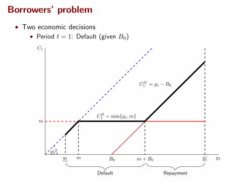
Borrowers’ problem
• Two economic decisions
• Period t = 1: Default (given B0)• Period t = 0: Borrowing B0

Borrowers’ problem
• Two economic decisions• Period t = 1: Default (given B0)
• Period t = 0: Borrowing B0

Borrowers’ problem
• Two economic decisions• Period t = 1: Default (given B0)• Period t = 0: Borrowing B0

Borrowers’ problem
• Two economic decisions• Period t = 1: Default (given B0)
• Period t = 0: Borrowing B0
C1
y1
45
y1 y1

Borrowers’ problem
• Two economic decisions• Period t = 1: Default (given B0)
• Period t = 0: Borrowing B0
C1
y1
45
y1 y1B0
CN1 = y1 −B0

Borrowers’ problem
• Two economic decisions• Period t = 1: Default (given B0)
• Period t = 0: Borrowing B0
C1
y1
45
y1 y1B0
CN1 = y1 −B0
mCD1 = miny1,m
Borrowers’ problem
• Two economic decisions• Period t = 1: Default (given B0)
• Period t = 0: Borrowing B0
C1
y1
45
y1 y1B0
CN1 = y1 −B0
mCD1 = miny1,m
m m+B0
Default Repayment

Borrowers’ problem
• Two economic decisions• Period t = 1: Default (given B0)
• Period t = 0: Borrowing B0
C1
y1
45
y1 y1B0
CN1 = y1 −B0
mCD1 = miny1,m
m m+B0
ForcedDefault
StrategicDefault

Borrowers’ problem
• Two economic decisions• Period t = 1: Default (given B0)• Period t = 0: Borrowing B0
U ′ (C0)
[q0 (B0,m) +
∂q0 (B0,m)
∂B0B0
]= β
∫ y1
m+B0
U ′ (y1 −B0) dF (y1)

Borrowers’ problem
• Two economic decisions• Period t = 1: Default (given B0)• Period t = 0: Borrowing B0
U ′ (C0)
[q0 (B0,m) +
∂q0 (B0,m)
∂B0B0
]= β
∫ y1
m+B0
U ′ (y1 −B0) dF (y1)
• Marginal Benefit: funds raised at t = 0 (accounting for price impact)• Marginal Cost: repayment at t = 1 only if no default

Borrowers’ problem
• Two economic decisions• Period t = 1: Default (given B0)• Period t = 0: Borrowing B0
U ′ (C0)
[q0 (B0,m) +
∂q0 (B0,m)
∂B0B0
]= β
∫ y1
m+B0
U ′ (y1 −B0) dF (y1)
• Marginal Benefit: funds raised at t = 0 (accounting for price impact)• Marginal Cost: repayment at t = 1 only if no default• Characterizes equilibrium borrowing (as a function of m)
B0(m)
dB0
dmR 0 (income, substitution and direct effects)

Lenders’ interest rate schedule
• Risk neutral pricing
q0 (B0,m) =δ∫m+B0
my1−mB0
dF (y1) +∫ y1m+B0
dF (y1)
1 + r∗
• Properties
∂q0 (B0,m)
∂B0< 0 and
∂q0 (B0,m)
∂m< 0
• More borrowing ⇒ Higher interest rates
• Higher exemptions ⇒ Higher interest rates
Eduardo Davila (NYU Stern) Optimal Bankruptcy Exemptions 7 / 16

Main Result 1: Marginal Change (directional test)
• Social welfare W (m) is given by borrowers utility
Eduardo Davila (NYU Stern) Optimal Bankruptcy Exemptions 8 / 16

Main Result 1: Marginal Change (directional test)
• Social welfare W (m) is given by borrowers utility
Marginal change in exemption
dW
dm= U ′ (C0)
∂q0
∂mB0
︸ ︷︷ ︸Marginal Cost: moreexpensive borrowing
+
∫ m+B0
mβU ′
(CD1)dF (y1)
︸ ︷︷ ︸Marginal Benefit: more
consumption when bankrupt
• Intuition• dB0
dm and changes in default decision do not appear• Borrowing and default are done optimally
Eduardo Davila (NYU Stern) Optimal Bankruptcy Exemptions 8 / 16
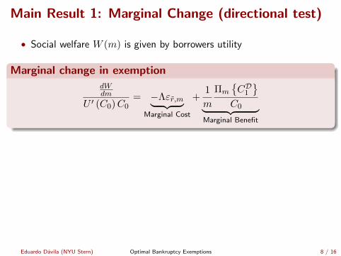
Main Result 1: Marginal Change (directional test)
• Social welfare W (m) is given by borrowers utility
Marginal change in exemptiondWdm
U ′ (C0)C0= −Λεr,m︸ ︷︷ ︸
Marginal Cost
+1
m
Πm
CD1
C0︸ ︷︷ ︸Marginal Benefit
Eduardo Davila (NYU Stern) Optimal Bankruptcy Exemptions 8 / 16

Main Result 1: Marginal Change (directional test)
• Social welfare W (m) is given by borrowers utility
Marginal change in exemptiondWdm
U ′ (C0)C0= −Λεr,m︸ ︷︷ ︸
Marginal Cost
+1
m
Πm
CD1
C0︸ ︷︷ ︸Marginal Benefit
Λ ≡ q0B0
y0 + q0B0Leverage
εr,m ≡∂ log (1 + r)
∂mInterest rate sensitivity
Eduardo Davila (NYU Stern) Optimal Bankruptcy Exemptions 8 / 16
Main Result 1: Marginal Change (directional test)
• Social welfare W (m) is given by borrowers utility
Marginal change in exemptiondWdm
U ′ (C0)C0= −Λεr,m︸ ︷︷ ︸
Marginal Cost
+1
m
Πm
CD1
C0︸ ︷︷ ︸Marginal Benefit
Πm
CD1
C0≡∫ m+B0
m
CD1C0
βU ′(CD1)
U ′ (C0)dF (y1) Price-Consumption ratio
Eduardo Davila (NYU Stern) Optimal Bankruptcy Exemptions 8 / 16

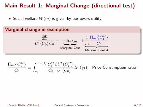
Main Result 1: Marginal Change (directional test)
• Social welfare W (m) is given by borrowers utility
Marginal change in exemptiondWdm
U ′ (C0)C0= −Λεr,m︸ ︷︷ ︸
Marginal Cost
+1
m
Πm
CD1
C0︸ ︷︷ ︸Marginal Benefit
Πm
CD1
C0≡∫ m+B0
m
CD1C0
βU ′(CD1)
U ′ (C0)dF (y1) Price-Consumption ratio
• Cash Flow and Discount Rate effects
Eduardo Davila (NYU Stern) Optimal Bankruptcy Exemptions 8 / 16
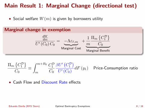

Main Result 1: Marginal Change (directional test)
• Social welfare W (m) is given by borrowers utility
Marginal change in exemptiondWdm
U ′ (C0)C0= −Λεr,m︸ ︷︷ ︸
Marginal Cost
+1
m
Πm
CD1
C0︸ ︷︷ ︸Marginal Benefit
Πm
CD1
C0≡∫ m+B0
m
CD1C0
βU ′(CD1)
U ′ (C0)dF (y1) Price-Consumption ratio
• Same formula for P/D ratios as in Consumption-Based AP
Eduardo Davila (NYU Stern) Optimal Bankruptcy Exemptions 8 / 16

Main Result 1: Marginal Change (directional test)
• Social welfare W (m) is given by borrowers utility
Marginal change in exemptiondWdm
U ′ (C0)C0= −Λεr,m︸ ︷︷ ︸
Marginal Cost
+1
m
Πm
CD1
C0︸ ︷︷ ︸Marginal Benefit
Πm
CD1
C0≡∫ m+B0
m
CD1C0
βU ′(CD1)
U ′ (C0)dF (y1) Price-Consumption ratio
• CRRA Utility:
Πm
CD1
C0= β
∫ m+B0
m
(CD1C0
)1−γ
dF (y1)
Eduardo Davila (NYU Stern) Optimal Bankruptcy Exemptions 8 / 16
Main Result 2: Optimal Exemption
• dWdm = 0 (under regularity conditions) ⇒ m∗
• Remarks
1. High Λεr,m and LowΠmCD
1 C0
⇒ Low m (and viceversa)2. Variables are endogenous and observable
• Sufficient statistic logic (CAPM analogy)• Similar to optimal taxation problems
3. Exact expression (no approximations)
Eduardo Davila (NYU Stern) Optimal Bankruptcy Exemptions 9 / 16

Main Result 2: Optimal Exemption
• dWdm = 0 (under regularity conditions) ⇒ m∗
Optimal exemption
m∗ =
ΠmCD1 C0
Λεr,m
• Remarks
1. High Λεr,m and LowΠmCD
1 C0
⇒ Low m (and viceversa)
2. Variables are endogenous and observable
• Sufficient statistic logic (CAPM analogy)• Similar to optimal taxation problems
3. Exact expression (no approximations)
Eduardo Davila (NYU Stern) Optimal Bankruptcy Exemptions 9 / 16

Main Result 2: Optimal Exemption
• dWdm = 0 (under regularity conditions) ⇒ m∗
Optimal exemption
m∗ =
ΠmCD1 C0
Λεr,m
• Remarks
1. High Λεr,m and LowΠmCD
1 C0
⇒ Low m (and viceversa)2. Variables are endogenous and observable
• Sufficient statistic logic (CAPM analogy)• Similar to optimal taxation problems
3. Exact expression (no approximations)
Eduardo Davila (NYU Stern) Optimal Bankruptcy Exemptions 9 / 16

Main Result 2: Optimal Exemption
• dWdm = 0 (under regularity conditions) ⇒ m∗
Optimal exemption
m∗ =
ΠmCD1 C0
Λεr,m
• Remarks
1. High Λεr,m and LowΠmCD
1 C0
⇒ Low m (and viceversa)2. Variables are endogenous and observable
• Sufficient statistic logic (CAPM analogy)• Similar to optimal taxation problems
3. Exact expression (no approximations)
Eduardo Davila (NYU Stern) Optimal Bankruptcy Exemptions 9 / 16

Figure: Social welfare
65 70 75 80 85 9088.92
88.94
88.96
88.98
89
89.02
89.04
89.06
89.08
89.1
89.12
W (m)
Exemption m
Welfare
Eduardo Davila (NYU Stern) Optimal Bankruptcy Exemptions 10 / 16
Extensions
1. Endogenous labor income and effort choice (moral hazard) M. Hazard
2. Non-pecuniary losses Utility loss
3. Epstein-Zin utility Epstein-Zin
4. Multiple contracts Multiple
5. Heterogeneous borrowers Heterogeneous
Eduardo Davila (NYU Stern) Optimal Bankruptcy Exemptions 11 / 16

Extensions
1. Endogenous labor income and effort choice (moral hazard) M. Hazard
2. Non-pecuniary losses Utility loss
3. Epstein-Zin utility Epstein-Zin
4. Multiple contracts Multiple
5. Heterogeneous borrowers Heterogeneous
• Social welfare function W =∫λ (i)W (i) dG (i)
m∗ =
EG,A[
Πm,iCD1i
C0i
]
EG,A [Λiεri,m]
• EG,A[·] are cross sectional averages (for active borrowers)• Observed heterogeneity: exclusion• Unobserved heterogeneity: pooling and exclusion
Eduardo Davila (NYU Stern) Optimal Bankruptcy Exemptions 11 / 16

Extensions
1. Endogenous labor income and effort choice (moral hazard) M. Hazard
2. Non-pecuniary losses Utility loss
3. Epstein-Zin utility Epstein-Zin
4. Multiple contracts Multiple
5. Heterogeneous borrowers Heterogeneous
6. Price taking borrowers Price taking
7. Bankruptcy exemptions contingent on aggregate risk Aggregate Risk
8. Endogenous income: labor wedges and aggregate demand Agg. demand
9. Dynamics Dynamics
Eduardo Davila (NYU Stern) Optimal Bankruptcy Exemptions 11 / 16

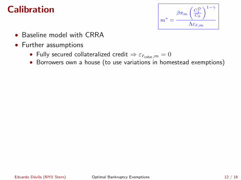
Calibrationm∗ =
βπm
(CD
1C0
)1−γ
Λεr,m
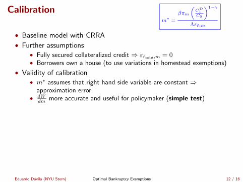
• Baseline model with CRRA
• Further assumptions• Fully secured collateralized credit ⇒ εrcollat,m = 0• Borrowers own a house (to use variations in homestead exemptions)
• Validity of calibration• m∗ assumes that right hand side variable are constant ⇒
approximation error• dW
dm more accurate and useful for policymaker (simple test)
Eduardo Davila (NYU Stern) Optimal Bankruptcy Exemptions 12 / 16
Calibrationm∗ =
βπm
(CD
1C0
)1−γ
Λεr,m
• Baseline model with CRRA
• Further assumptions• Fully secured collateralized credit ⇒ εrcollat,m = 0• Borrowers own a house (to use variations in homestead exemptions)
• Validity of calibration• m∗ assumes that right hand side variable are constant ⇒
approximation error• dW
dm more accurate and useful for policymaker (simple test)
Eduardo Davila (NYU Stern) Optimal Bankruptcy Exemptions 12 / 16

Calibrationm∗ =
βπm
(CD
1C0
)1−γ
Λεr,m
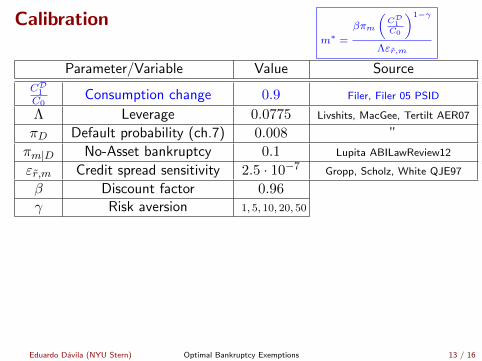
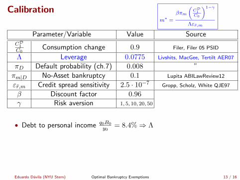
Parameter/Variable Value SourceCD1C0
Consumption change 0.9 Filer, Filer 05 PSID
Λ Leverage 0.0775 Livshits, MacGee, Tertilt AER07
πD Default probability (ch.7) 0.008 ”
πm|D No-Asset bankruptcy 0.1 Lupita ABILawReview12
εr,m Credit spread sensitivity 2.5 · 10−7 Gropp, Scholz, White QJE97
β Discount factor 0.96γ Risk aversion 1, 5, 10, 20, 50
Eduardo Davila (NYU Stern) Optimal Bankruptcy Exemptions 13 / 16
Calibrationm∗ =
βπm
(CD
1C0
)1−γ
Λεr,m
Parameter/Variable Value SourceCD1C0
Consumption change 0.9 Filer, Filer 05 PSID
Λ Leverage 0.0775 Livshits, MacGee, Tertilt AER07
πD Default probability (ch.7) 0.008 ”
πm|D No-Asset bankruptcy 0.1 Lupita ABILawReview12
εr,m Credit spread sensitivity 2.5 · 10−7 Gropp, Scholz, White QJE97
β Discount factor 0.96γ Risk aversion 1, 5, 10, 20, 50
• Debt to personal income q0B0
y0= 8.4%⇒ Λ
Eduardo Davila (NYU Stern) Optimal Bankruptcy Exemptions 13 / 16

Calibrationm∗ =
βπm
(CD
1C0
)1−γ
Λεr,m
Parameter/Variable Value SourceCD1C0
Consumption change 0.9 Filer, Filer 05 PSID
Λ Leverage 0.0775 Livshits, MacGee, Tertilt AER07
πD Default probability (ch.7) 0.008 ”
πm|D No-Asset bankruptcy 0.1 Lupita ABILawReview12
εr,m Credit spread sensitivity 2.5 · 10−7 Gropp, Scholz, White QJE97
β Discount factor 0.96γ Risk aversion 1, 5, 10, 20, 50
• πm = πD︸︷︷︸0.008
×πm|D︸ ︷︷ ︸0.1
(zero recovery by unsecured creditors ≈ 90%)
Eduardo Davila (NYU Stern) Optimal Bankruptcy Exemptions 13 / 16

Calibrationm∗ =
βπm
(CD
1C0
)1−γ
Λεr,m
Parameter/Variable Value SourceCD1C0
Consumption change 0.9 Filer, Filer 05 PSID
Λ Leverage 0.0775 Livshits, MacGee, Tertilt AER07
πD Default probability (ch.7) 0.008 ”
πm|D No-Asset bankruptcy 0.1 Lupita ABILawReview12
εr,m Credit spread sensitivity 2.5 · 10−7 Gropp, Scholz, White QJE97
β Discount factor 0.96γ Risk aversion 1, 5, 10, 20, 50
• Increasing m by $100,000, increases credit spread by 250 basis points
Eduardo Davila (NYU Stern) Optimal Bankruptcy Exemptions 13 / 16

Calibrationm∗ =
βπm
(CD
1C0
)1−γ
Λεr,m
Parameter/Variable Value SourceCD1C0
Consumption change 0.9 Filer, Filer 05 PSID
Λ Leverage 0.0775 Livshits, MacGee, Tertilt AER07
πD Default probability (ch.7) 0.008 ”
πm|D No-Asset bankruptcy 0.1 Lupita ABILawReview12
εr,m Credit spread sensitivity 2.5 · 10−7 Gropp, Scholz, White QJE97
β Discount factor 0.96γ Risk aversion 1, 5, 10, 20, 50
Eduardo Davila (NYU Stern) Optimal Bankruptcy Exemptions 13 / 16

Calibration
m∗ =
βπm
(CD
1C0
)1−γ
Λεr,m
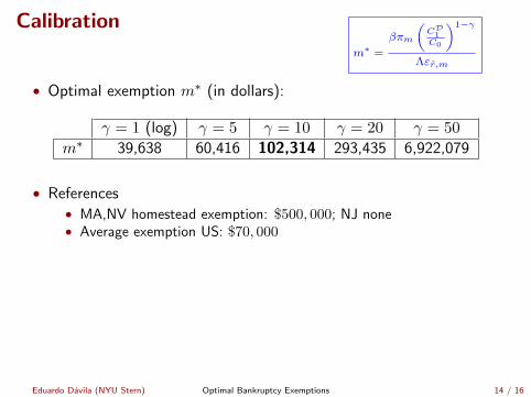
• Optimal exemption m∗ (in dollars):
γ = 1 (log) γ = 5 γ = 10 γ = 20 γ = 50
m∗ 39,638 60,416 102,314 293,435 6,922,079
• References• MA,NV homestead exemption: $500, 000; NJ none• Average exemption US: $70, 000
• Size of welfare gains at $70, 000 using dWdm formula ($10, 000 change)
γ = 1 (log) γ = 5 γ = 10 γ = 20 γ = 50dWdm
U ′(C0)C0-0.0084% -0.0027% 0.0089% 0.062% 1.897%
Eduardo Davila (NYU Stern) Optimal Bankruptcy Exemptions 14 / 16
Calibration
m∗ =
βπm
(CD
1C0
)1−γ
Λεr,m
• Optimal exemption m∗ (in dollars):
γ = 1 (log) γ = 5 γ = 10 γ = 20 γ = 50
m∗ 39,638 60,416 102,314 293,435 6,922,079
• References• MA,NV homestead exemption: $500, 000; NJ none• Average exemption US: $70, 000
• Size of welfare gains at $70, 000 using dWdm formula ($10, 000 change)
γ = 1 (log) γ = 5 γ = 10 γ = 20 γ = 50dWdm
U ′(C0)C0-0.0084% -0.0027% 0.0089% 0.062% 1.897%
Eduardo Davila (NYU Stern) Optimal Bankruptcy Exemptions 14 / 16

Calibration dWdm
U ′ (C0)C0= −Λεr,m +
1
mβπm
(CD1C0
)1−γ
• Optimal exemption m∗ (in dollars):
γ = 1 (log) γ = 5 γ = 10 γ = 20 γ = 50
m∗ 39,638 60,416 102,314 293,435 6,922,079
• References• MA,NV homestead exemption: $500, 000; NJ none• Average exemption US: $70, 000
• Size of welfare gains at $70, 000 using dWdm formula ($10, 000 change)
γ = 1 (log) γ = 5 γ = 10 γ = 20 γ = 50dWdm
U ′(C0)C0-0.0084% -0.0027% 0.0089% 0.062% 1.897%
Eduardo Davila (NYU Stern) Optimal Bankruptcy Exemptions 14 / 16

Literature
1. Sufficient Statistics/Public Economics: Diamond 98, Saez 01,Shimer-Werning 07, Chetty 09, Arkolakis et al 12
2. General Equilibrium with Incomplete Markets: Zame 93,Dubey-Geanakoplos-Shubik 05
3. Quantitative Literature:• Structural: Chatterjee-Corbae-Nakajima-Rios-Rull 07,
Livshits-MacGee-Tertilt 07,• Microeconometric: Gross-Souleles 02, Fay-Hurst-White 02, Fan-
White 03, Severino-Brown-Coates 14
4. Security Design: Ross 76, Allen-Gale 94, Duffie-Rahi 95
5. Optimal Contracting: many papers
Eduardo Davila (NYU Stern) Optimal Bankruptcy Exemptions 15 / 16
Conclusion
1. This paper has characterized optimal bankruptcy exemptions• As a function of a few sufficient statistics• For a wide range of environments• Sensible calibration (measurement is challenging)
2. New paper on mortgage design (with John Campbell)• Optimal recourse• ARM vs FRM
Eduardo Davila (NYU Stern) Optimal Bankruptcy Exemptions 16 / 16

Figures: Interest rate schedule
25 30 35 40 450.72
0.74
0.76
0.78
0.8
0.82
0.84
0.86
0.88
0.9
q0 (B0,m)
Loan Size B0
Price
65 70 75 80 85 900.882
0.884
0.886
0.888
0.89
0.892
0.894
0.896
0.898
0.9
0.902
q0 (B0,m)
Exemption m
Price
Eduardo Davila (NYU Stern) Optimal Bankruptcy Exemptions 17 / 16

Figures: Borrowers’ choices
25 30 35 40 4587
87.5
88
88.5
89
89.5
J (B0,m)
Loan Size B0
Welfare
65 70 75 80 85 9027
28
29
30
31
32
33
34
35
B0 (m)
Exemption m
LoanSize
Eduardo Davila (NYU Stern) Optimal Bankruptcy Exemptions 18 / 16

Extensions
1. Endogenous labor income and effort choice (moral hazard) M. Hazard
Eduardo Davila (NYU Stern) Optimal Bankruptcy Exemptions 19 / 16

Extensions
1. Endogenous labor income and effort choice (moral hazard) M. Hazard
• Same expression for m∗ if disutility of labor is separable (frictionlesslabor markets)
• Different characterization of default region: does not matter for m∗
(insight applies more generally)• Intuition: optimality
Eduardo Davila (NYU Stern) Optimal Bankruptcy Exemptions 19 / 16
Extensions
1. Endogenous labor income and effort choice (moral hazard) M. Hazard
2. Non-pecuniary losses Utility loss
Eduardo Davila (NYU Stern) Optimal Bankruptcy Exemptions 19 / 16

Extensions
1. Endogenous labor income and effort choice (moral hazard) M. Hazard
2. Non-pecuniary losses Utility loss
• Same expression for m∗
• Effects work through spreads in εr,m and default regions• Implicit assumption: no renegotiation• Easy to add externalities/internalities
Eduardo Davila (NYU Stern) Optimal Bankruptcy Exemptions 19 / 16

Extensions
1. Endogenous labor income and effort choice (moral hazard) M. Hazard
2. Non-pecuniary losses Utility loss
3. Epstein-Zin utility Epstein-Zin
Eduardo Davila (NYU Stern) Optimal Bankruptcy Exemptions 19 / 16

Extensions
1. Endogenous labor income and effort choice (moral hazard) M. Hazard
2. Non-pecuniary losses Utility loss
3. Epstein-Zin utility Epstein-Zin
• Same expression for m∗
Πm
CD1
C0≡(Q
C0
)γ− 1ψ
β
∫ m+B0
m
(CD1C0
)1−γ
dF (y1)
• Where Q is the certainty equivalent of t = 1 consumption
Eduardo Davila (NYU Stern) Optimal Bankruptcy Exemptions 19 / 16

Extensions
1. Endogenous labor income and effort choice (moral hazard) M. Hazard
2. Non-pecuniary losses Utility loss
3. Epstein-Zin utility Epstein-Zin
• Same expression for m∗
Πm
CD1
C0≡(Q
C0
)γ− 1ψ
β
∫ m+B0
m
(CD1C0
)1−γ
dF (y1)
• Where Q is the certainty equivalent of t = 1 consumption• Corrected Stochastic Discount Factor
Eduardo Davila (NYU Stern) Optimal Bankruptcy Exemptions 19 / 16

Extensions
1. Endogenous labor income and effort choice (moral hazard) M. Hazard
2. Non-pecuniary losses Utility loss
3. Epstein-Zin utility Epstein-Zin
4. Multiple contracts Multiple
Eduardo Davila (NYU Stern) Optimal Bankruptcy Exemptions 19 / 16

Extensions
1. Endogenous labor income and effort choice (moral hazard) M. Hazard
2. Non-pecuniary losses Utility loss
3. Epstein-Zin utility Epstein-Zin
4. Multiple contracts Multiple
• Optimal exemption
m∗ =
ΠmCD1
C0∑Jj=1 Λjεrj ,m
Λj ≡q0jB0j
y0 +∑Jj=1 q0jB0j
• Complete markets as special case ⇒ m∗ = 0
Eduardo Davila (NYU Stern) Optimal Bankruptcy Exemptions 19 / 16

Extensions
1. Endogenous labor income and effort choice (moral hazard) M. Hazard
2. Non-pecuniary losses Utility loss
3. Epstein-Zin utility Epstein-Zin
4. Multiple contracts Multiple
5. Heterogeneous borrowers Heterogeneous
Eduardo Davila (NYU Stern) Optimal Bankruptcy Exemptions 19 / 16

Extensions
1. Endogenous labor income and effort choice (moral hazard) M. Hazard
2. Non-pecuniary losses Utility loss
3. Epstein-Zin utility Epstein-Zin
4. Multiple contracts Multiple
5. Heterogeneous borrowers Heterogeneous
• Social welfare function W =∫λ (i)W (i) dG (i)
m∗ =
EG,A[
Πm,iCD1i
C0i
]
EG,A [Λiεri,m]
• EG,A[·] are cross sectional averages (for active borrowers)• Observed heterogeneity: exclusion• Unobserved heterogeneity: pooling and exclusion
Eduardo Davila (NYU Stern) Optimal Bankruptcy Exemptions 19 / 16

Extensions
1. Endogenous labor income and effort choice (moral hazard) M. Hazard
2. Non-pecuniary losses Utility loss
3. Epstein-Zin utility Epstein-Zin
4. Multiple contracts Multiple
5. Heterogeneous borrowers Heterogeneous
6. Price taking borrowers Price taking
• Euler equation
U ′ (C0) q0 = β
∫ y1
φm+B0
U ′(CN1
)dF (y1)
• Optimal exemption
m∗ =
ΠmCD1
C0
Λεr,mwhere εr,m =
d log(1 + r)
dm
• Full GE effect
Eduardo Davila (NYU Stern) Optimal Bankruptcy Exemptions 19 / 16

Extensions
1. Endogenous labor income and effort choice (moral hazard) M. Hazard
2. Non-pecuniary losses Utility loss
3. Epstein-Zin utility Epstein-Zin
4. Multiple contracts Multiple
5. Heterogeneous borrowers Heterogeneous
6. Price taking borrowers Price taking
7. Bankruptcy exemptions contingent on aggregate risk Aggregate Risk
• Aggregate shocks ω ∈ Ω, we can condition exemptions on those
m∗ (ω) =
Πm(ω)CD1 C0
Λεr,m(ω), ∀ω
Eduardo Davila (NYU Stern) Optimal Bankruptcy Exemptions 19 / 16

Extensions
1. Endogenous labor income and effort choice (moral hazard) M. Hazard
2. Non-pecuniary losses Utility loss
3. Epstein-Zin utility Epstein-Zin
4. Multiple contracts Multiple
5. Heterogeneous borrowers Heterogeneous
6. Price taking borrowers Price taking
7. Bankruptcy exemptions contingent on aggregate risk Aggregate Risk
8. Endogenous income: labor wedges and aggregate demand Agg. demand
m∗ =
ΠmCD1 C0
+ΠN
τ(ω)
dY (ω)dmm
C0
Λεr,m
• Where 1 + τ(ω) = w1(ω)A is the labor wedge
Eduardo Davila (NYU Stern) Optimal Bankruptcy Exemptions 19 / 16

Extensions
1. Endogenous labor income and effort choice (moral hazard) M. Hazard
2. Non-pecuniary losses Utility loss
3. Epstein-Zin utility Epstein-Zin
4. Multiple contracts Multiple
5. Heterogeneous borrowers Heterogeneous
6. Price taking borrowers Price taking
7. Bankruptcy exemptions contingent on aggregate risk Aggregate Risk
8. Endogenous income: labor wedges and aggregate demand Agg. demand
9. Dynamics Dynamics
m∗ =
∑Tt=1
Πm,tCDt C0∑T−1
t=0 ΠN ,t gtΛtεrt,m• Simple formula interpreted as steady state• Income process subsumed in sufficient statistics (permanent vs.
transitory shocks, health shocks, family shocks, etc...)
Eduardo Davila (NYU Stern) Optimal Bankruptcy Exemptions 19 / 16

Sign of dB0
dm
sign
(U ′′ (C0)
∂q0
∂mB0
[q0 +
∂q0
∂B0B0
]+ U ′ (C0)
[∂q0
∂m+
∂2q0
∂B0∂mB0
]
+ βU ′ (m) f (m+B0))
Back to text
Eduardo Davila (NYU Stern) Optimal Bankruptcy Exemptions 20 / 16

m∗ in (almost) closed form
m∗ =
(β (1 + r∗)
Υ + δ (1−Υ)
) 1γ
C0
Υ =f (m∗ +B0)B0
F (m∗ +B0)− F (m∗)
• Υ = 1 for uniform (measure of curvature)
Back to text
Eduardo Davila (NYU Stern) Optimal Bankruptcy Exemptions 21 / 16

Moral Hazard/Elastic Labor Supply
• Borrowers’ problem
maxC0,C1y1 ,B0,ξy1 ,N0,N1y1 ,a
U (C0, N0; a) + βEa [U (C1, N1)]
s.t. C0 = y0 + w0N0 + q0B0
CN1 = y1 + w1NN1 −B0; CD1 = min y1,m
• Two new optimality conditions
∂U
∂a(C0, N0; a) + β
∫V (C1, N1) fa (y1; a) dy1 = 0
w0∂U
∂C(C0, N0; a) = − ∂U
∂N(C0, N0; a)
• Same m∗
Back to text
Eduardo Davila (NYU Stern) Optimal Bankruptcy Exemptions 22 / 16

Moral Hazard/Elastic Labor Supply: DefaultDecision
U (·)
Income
U (m)
m y1y1 y1
U (y1; 0) V(y1;B
b0, w1
)
U (m)
Eduardo Davila (NYU Stern) Optimal Bankruptcy Exemptions 23 / 16
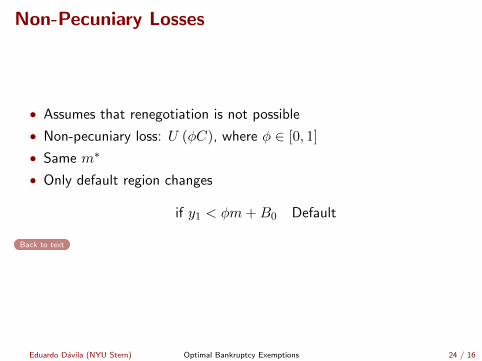
Non-Pecuniary Losses
• Assumes that renegotiation is not possible
• Non-pecuniary loss: U (φC), where φ ∈ [0, 1]
• Same m∗
• Only default region changes
if y1 < φm+B0 Default
Back to text
Eduardo Davila (NYU Stern) Optimal Bankruptcy Exemptions 24 / 16

Borrowers Internalize Price Response
• Borrowers optimality condition
U ′ (C0)
[q0 +
∂ql0∂B0
Bb0
]= β
∫ y1
φm+Bb0
U ′(CN1)dF (y1)
• Optimal exemption
m∗ =
ΠmCD1 C0
Λ(εr,m + εB0,mεql0,B0
)
where εB0,m ≡dB0B0dm , εql0,B0
≡∂ql0q0
∂Bb0B0
Back to text
Eduardo Davila (NYU Stern) Optimal Bankruptcy Exemptions 25 / 16

Epstein-Zin
• Only difference: stochastic discount factor
• m∗ doesn’t change but
Πm
CD1
C0≡(Q
C0
)γ− 1ψ
β
∫ m+B0
m
(CD1C0
)1−γ
dF (y1)
• Q is the certainty equivalent of consumption
Q ≡(∫ m
y1
(y1)1−γ dF (y1) +
∫ m+Bb0
m(m)1−γ dF (y1) +
∫ y1
m+B0
(y1 −B0)1−γ dF (y1)
) 11−γ
,
Back to text
Eduardo Davila (NYU Stern) Optimal Bankruptcy Exemptions 26 / 16

Multiple Arbitrary Contracts
• Budget constraints
C0 = y0 +
J∑
j=1
q0j (B01,...B0J ,m)B0j
CN1 = y1 +
J∑
j=1
max −zj (y1)B0j , 0 −J∑
j=1
max zj (y1)B0j , 0
CD1 = min
y1 +
J∑
j=1
max −zj (y1)B0j , 0 ,m
• Weighted sum of elasticities
m∗ =
ΠmCD1 C0∑J
j=1 Λjεrj ,m
Back to text
Eduardo Davila (NYU Stern) Optimal Bankruptcy Exemptions 27 / 16

Multiple Arbitrary Contracts
C1
y1
m
Dyy1 y1Dm
CN1 = y1 +∑J
j=1 max −zj (y1)B0j , 0 −∑J
j=1 max zj (y1)B0j , 0
CD1 = miny1 +
∑Jj=1 max −zj (y1)B0j , 0 ,m
y1 +∑J
j=1 max −zj (y1)B0j , 0
maxCD1 , CN1
45
NEduardo Davila (NYU Stern) Optimal Bankruptcy Exemptions 28 / 16

Heterogeneous borrowers (observed heterogeneity)
q0i (B0i,m) =
11+r∗ , B0i ≤ 0δ∫m+B0im
y1i−mB0i
dFi(y1i)+∫ y1im+B0i
dFi(y1i)
1+r∗ , B0i > 0
IA (m) = i|B0i (m) > 0 , Active borrowers
IN (m) = i|B0i (m) = 0 , Inactive borrowers
Back to text
Eduardo Davila (NYU Stern) Optimal Bankruptcy Exemptions 29 / 16
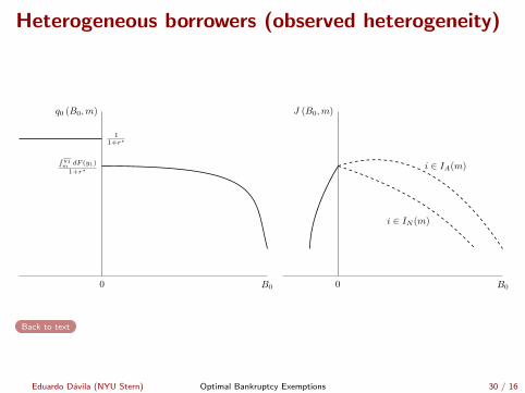
Heterogeneous borrowers (observed heterogeneity)
0
q0 (B0,m)
B0
11+r∗
∫ y1m
dF (y1)
1+r∗
0
J (B0,m)
B0
i ∈ IA(m)
i ∈ IN (m)
Back to text
Eduardo Davila (NYU Stern) Optimal Bankruptcy Exemptions 30 / 16

Heterogeneous borrowers (observed heterogeneity)
q0i (B0,m) =
11+r∗ , B0i ≤ 0∫IA(m)
q0i(B0,m)∫IA(m) dG(i)
dG (i) , B0i > 0,
where
q0i (B0,m) =δ∫m+B0
my1i−mB0
dFi (y1i) +∫ y1im+B0
dFi (y1i)
1 + r∗
Back to text
Eduardo Davila (NYU Stern) Optimal Bankruptcy Exemptions 31 / 16
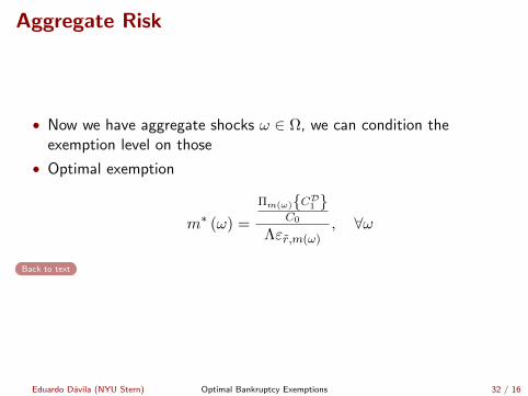
Aggregate Risk
• Now we have aggregate shocks ω ∈ Ω, we can condition theexemption level on those
• Optimal exemption
m∗ (ω) =
Πm(ω)CD1 C0
Λεr,m(ω), ∀ω
Back to text
Eduardo Davila (NYU Stern) Optimal Bankruptcy Exemptions 32 / 16

Dynamics
• Borrowers maximize maxE[∑T
t=0 βtU (Ct)
]
• Recursively VND,0 (B−1, y0;m) =maxB0 U (C0) + βE [max VND,1 (B0, y1;m) , VD,1 (y1;m)]
• Optimal exemption
m∗ =
∑Tt=1
ΠmCDt C0∑T−1
t=0 ΠND gtΛtεrt,m
• Easy to allow for default before bankruptcy, wage garnishments,exclusion period
Back to text
Eduardo Davila (NYU Stern) Optimal Bankruptcy Exemptions 33 / 16

Evolution filings US
Back to text
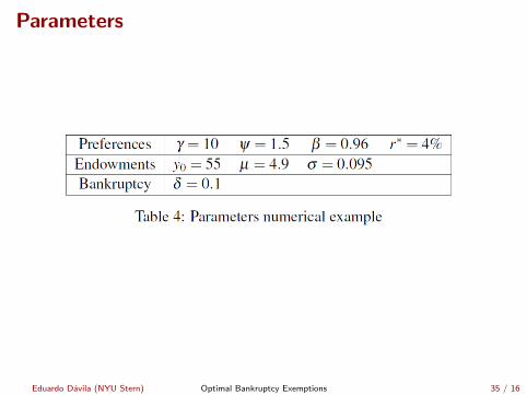
Parameters
Eduardo Davila (NYU Stern) Optimal Bankruptcy Exemptions 35 / 16
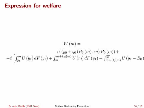
Expression for welfare
W (m) =
U (y0 + q0 (B0 (m) ,m)B0 (m)) +
+β[∫my1U (y1) dF (y1) +
∫m+B0(m)m U (m) dF (y1) +
∫ y1m+B0(m) U (y1 −B0 (m)) dF (y1)
],
Eduardo Davila (NYU Stern) Optimal Bankruptcy Exemptions 36 / 16