Using Discrete Programming

By Clark Edwards

• In many important economic problems, a variable is maximized subject to constraints. In a subset of such problems, a linear combination of decision vari-ables is maximized subject to linear constraints. The latter subset is amenable to linear programming analysis. Efforts to expand the usefulness of linear programming methods usually involve incorporat-ing nonlinear elements either in the criterion func-tion or in the constraints. Such efforts frequently result in discovering ways to incorporate the non-linear element in some acceptable linear form, thus retaining the usual linear programming procedure but broadening the researcher's capacity to apply the method to important economic problems (9).1 Dis-crete programming is a case in point. Discrete pro-gramming problems and ordinary linear program-ming problems are about the same, except that a side

ilk condition is imposed that some of the decision vari-ables must take on discrete values, usually nonnega-tive integers. The resultant, noncontinuous nature of the criterion function or of the constraints places discrete programming in the class of nonlinear pro-gramming (10). Sufficient conditions for a solution to discrete programming problems have been known for several years (15). Recently, systematic proce-dures for solving discrete programming problems have been put forward (14, 16). This paper dis-cusses one of them. Decks and tapes for solving such problems on high-speed computers are not yet abundant, but it would be easy to supply them should the demand arise.

A LINEAR PROGRAMMING problem is one A in which elements of a decision vector x are to be chosen in such a way as to maximize Q (1) Q=c'x subject to (2) Ax-b and to (3) x0

1 Italic numbers in parentheses refer to Literature Cited

eland Selected References, p. 59.

Integer programming is done under the addi-tional constraint that (4) some elements of x are integers.

If Q is net revenue in a farm management prob-lem and xi is the swine activity, to insist by (4) that xi be an integer is simply to require that if some sows are to be farrowed in the optimal farm plan, an integral number must be farrowed. If, without the discrete restriction, the optimal num-ber of sows were estimated at 17.682, the question arises (in this case, perhaps, a somewhat trivial question) as to whether some limited resources should be withdrawn from other activities to in-crease sow numbers to 18 (or 19) or whether it would be more profitable to farrow 17 (or 16) sows and release some limited resources for other uses.

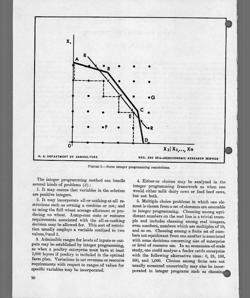
Some integer programming restrictions are shown in figure 1. Line ABCD represents the feasible, noninteger boundary for pairs of x1 and x2 given levels for activities x3 to xn. Inside ABCD, the boundary for integer pairs of values is marked with a dotted line. With RR depicting the price ratio, or choice indicator, B marks the high profit point of the noninteger solution. E marks the high profit point for x1 and x2 integers but x3 to xn held constant. In a simultaneous integer solution of all n activities, the optimal level of, say, x, might change sufficiently that the best combination of x1 and x2 would shift away from E, say, to F or G.

The marginal utility of adding a discrete restriction to a programming problem may be negligible when the magnitude of the decision variable is large relative to the size of the dis-crete jump. For example, it may be less interest-ing to know if a number like 103.467 should round up to 104 or down to 103 than to know if a num-ber like 0.674 should round up to 1.0 or down to zero. It is the systematic way in which discrete programming handles relatively large jumps that makes it useful and interesting.

49 680439--63---2

U. S. DEPARTMENT OF AGRICULTURE NEG. ERS 1816-63(2)ECONOMIC RESEARCH SERVICE

X 2 1 X 3,.. n

FIGURE 1.—Some integer programming restrictions.

The integer programming method can handle several kinds of problems (8) :

1. It may ensure that variables in the solution are positive integers.

2. It may incorporate all-or-nothing-at-all re-strictions such as owning a combine or not; and as using the full wheat acreage allotment or pro-ducing no wheat. Lump-sum costs or resource requirements associated with the all-or-nothing decision may be allowed for. This sort of restric-tion usually employs a variable confined to two values, 0 and 1.

3. Admissible ranges for levels of inputs or out-puts may be established by integer programming, as when a poultry enterprise must have at least 1,000 layers if poultry is included in the optimal farm plan. Variations in net revenues or resource requirements with respect to ranges of values for specific variables may be incorporated.

50

4. Either-or choices may be analyzed in the integer programming framework as when one would either milk dairy cows or feed beef cows, but not both.

5. Multiple choice problems in which one ele-ment is chosen from a set of elements are amenable to integer programming. Choosing among equi-distant numbers on the real line is a trivial exam-ple and includes choosing among real integers, even numbers, numbers which are multiples of 10, and so on. Choosing among a finite set of num-bers not equidistant from one another is associated with some decisions concerning size of enterprise or level of resource use. In an economies-of-scale study, one could analyze a feeder cattle enterprise with the following alternative sizes : 0, 25, 100, 500, and 1,000. Choices among finite sets not usually measured numerically may also be incor-porated in integer programs such as choosing

among five crop rotations considered for a farm;

Sr, choosing among three feeding methods con-sidered for a hog enterprise.

Writing the Discrete Restrictions

Writing a discrete restriction in a program-ming problem frequently involves devising a scheme for restating a nonlinear, discontinuous problem in a linear, continuous form, equations (1), (2), and (3), and then imposing the added restriction that one or more variables are integers, equation (4). Some examples follow :

Example 1.—Let xi be acres of corn and xk a (0,1) variable representing a fixed complement of machinery and equipment necessary for handling a corn crop. Net revenue, equation (1), includes the terms

(5)

eiXj +CkXk

where ck is the annual cost of making the machin-ery and equipment available and cj is the change in net revenue associated with growing an acre of corn given that the machinery has been made available.

A complete statement of the corn-machinery

(

froblem could include the statement that

which says that if corn is grown, machinery must be made available, and if machinery is not made available, corn can not be grown. That machin-ery might be made available without growing corn is feasible according to (6) but not economic according to (5). Growing corn without equip-ment is not feasible according to (6).

While (6) states the discrete restriction, it is not in the form of equation (2) and is not amen-able to ordinary programming procedures. The restriction may be translated to a usable form by introducing a dummy parameter based on the knowledge that the variable xi has an upper bound imposed by other constraints to the prob-lem. For instance, one of the restrictions in (2) may state that only 100 acres of corn land are available in which case any real number not less than 100 may be used as an upper bound for xj. Let us call the dummy parameter ai. Now we write the restriction (7) xi-<-ccixk

•

xk an integer

which conforms to (2) and (4) and can be shown to satisfy (6). The terms (5) would appear in equation (1) and the inequality in (7) would appear as one of the equations in (2). According to (7), it is not feasible to grow corn unless machinery is made. available. If corn is not grown on the farm, the profit maximizing criterion requires that no machinery is made available. If corn is grown, then (7) requires that at least one set be made available and the profit maximizing criterion requires that not more than one set of machinery is acquired. Thus xk will be either 0 or 1 in the optimal solution. Many enterprises require an initial, overhead cost in addition to a variable, unit cost. Discrete programming is an efficient way to distribute fixed charges. The term ckxk in (5) represents a fixed charge in terms of a cash outlay, or a lump sum reduction in net revenue.

If the fixed cost were measured in terms of using up a lump sum of limited resources such as building space or labor, rather than in terms of directly reducing net revenue, a similar restric-tion results. Interpreting (7) as above, set ck =0 to show that net revenue is not directly affected by a change in the (0,1) variable, xk. Then, let-ting the PI equation in (2) represent the labor restriction, let au, reflect the fixed labor require-ment. See appendix table 1, line 5, for an illus-tration. Now if xk =1 the fixed labor supply is reduced by aik, but if xk=0 the labor supply is not affected.

Example 2.—In example 1, the discrete variable takes one of two values : 0 and 1. In other prob-lems, the discrete variable may assume any non-negative integer. For instance, perhaps the number of storage bins is to be an integer and there must be at least one bin for each 10,000 bushels of grain; or the number of machines employed in an activity must be an integer and there must be at least 1 machine for each 10 units of labor.

Let xi be an activity providing labor and xk one providing machines and suppose the number of machines supplied must be an integer. The supplies of xi and xk may be perfectly elastic with unit costs represented by cj and ck. In this event, neither variable would have an upper bound as did the variable in the previous example. Appro-priate coefficients in the labor restriction equation would ensure that an adequate quantity of labor,

51

6) x j>0-->xk=1

xj, is made available. In addition, an equation saying that xj--axk as in equation (7), will ensure that there will be at least one machine for each a units of labor. Hence, while other restrictions in (2) would lead to the optimal labor utilization, (7) would ensure an adequate supply of machinery.

Example 3.—Sometimes it is desirable to impose the restriction that if an activity is used, it is used at least at a minimal level. For instance, if wheat is to be grown then at least 15 acres must be grown; and, if cows are to be milked then at least 25 head must be in the herd. Let us say that for a dairy activity, x j, it is known from other con-straints in the problem that 100 is an upper bound for x j. Furthermore, we know from prior economic analysis that if there is to be a dairy activity in the final solution, the herd must have at least 25 cows. That is, we wish to impose

(8) either 25-xj-100 or xj=0

This nonlinear, discontinuous condition can be written in a form suitable for ordinary program-ming methods by writing

(9) Xi '13j xk xk an integer

where a j is the upper bound, 100, and Si is the lower bound, 25. If introducing the first 25 cows involved an overhead cost, this could be reflected by a value for ck in the profit equation. If the first 25 cows affected the ith restriction differently from the additional cows, as by requiring a lump sum labor requirement in addition to the variable labor requirement per cow, this could be reflected by a value for aik in the ith equation of (2). In (9), it follows that if xk = 0, xj =0. If xk = 1, 25---x j -100 as required in (8). An uneconomic-size herd of, say, 10 head is not feasible because xj =10 violates the first inequality of (9) if xk=0 and violates the second inequality if xk=1.

Example 4.—Discrete variables may assume one of several values which are not equidistant from one another. One might want to consider wheat acreages of 0, 15, and 40 acres or consider dairy enterprises of 0-, 25-, 60-, and 100-cow herds with-out examining other activity levels. In the dairy example, each herd size may be considered efficient for alternative sets of buildings and equipment,

52

qualities of cows, rates of feeding, and require- ments of labor.

A restriction of the form (10) xj =25xk+ 60xm -I- 100x.

xk, xm, xn are integers would permit examination of the four dairy alter-natives. If each of the integer variables were zero, x j would also be zero.

If, in the profit maximizing process, more than one herd appeared in the final solution and at most one herd was considered admissible, the further restriction would be imposed that (11) 1xk + xm+ xi, Forcing the equality in (11) would result in exactly one herd and allowing the inequality would allow none. Frequently, an equation of type (11) will not be violated even when not explicitly imposed due to the nature of the cri-terion function (1) and to other restrictions in (2).

As in prior examples, values for ck, cm, cn, ant, aim, and ain may be incorporated to account for lump sum increments in costs, returns, or resource use associated with alternative levels of xj.

Example 5.—If a farm organization could in-clude either Herefords or Holsteins but not both, farrow either one litter of pigs per year or twill, litters but not both, or plant either corn or soy-beans in a field but not both, then a restriction of the form (12) xi •xj=0 would require that at least one of the activities not enter into the solution. This nonlinear condi-tion may be imposed by two linear inequalities in an integer program. Let al and a j be upper bounds for xi and xj, respectively. Such bounds are always implied by other constraints in (2). Then incorporate the restriction that

Xi .. aiXk (13) xj a j (1 — xk)

xk an integer with the understanding that xk is confined to the integers 0 and 1. Should difficulties in computa-tion arise from xk--2, simply impose the addi-tional restriction that xk-1. See appendix table 1, lines 6 and 7, for an illustration.

Displaying the Discrete Solution

Let the integer programming problem be stated in the form of equations (1) to (4) with (20

•

including equations such as (7), (9), (10) and

W13). The first step in displaying the integer olution is to solve equations (1), (2), and (3),

ignoring (4) to get a first approximation (14). The first approximation allows variables which

are supposed to be integers to take on noninteger values and therefore need not be a feasible solu-tion. For example, one of the (0,1) variables might have the value of .90 in the first approxi-mation. This might mean that only 90 percent of a combine or 90 percent of a dairy barn is allowed for in the solution. The next step is to add an additional equation to the noninteger solu-tion matrix, incorporating information as to which of the variables are to be integers, and to proceed with the computations.

The rules for discrete programming are simpler if equation (4) is changed to read "all x1 are in-tegers." Let us examine first the complete integer solution and then take up the partial integer solution.

The Complete Integer Solution Let equation (14) represent the ith of m restric-

tions in the first approximation, or the noninteger solution of a linear program for which an integer

f olution is desired.

(14) E alixi=b, (1 <i<m) S=1

where it is understood that au=1

for the coefficient of the x j having the value b1 in the current basis, say xk

(15) au =0 for coefficients of all other xi included in the current basis

— co <am< co for coefficients of all x j not included in the current basis

Some of the x j in (14) are real activities, some are slack variables and others were introduced through equations such as (7). Any of the m equations may be chosen for (14) provided bi is not, in fact, an integer in the first approximation. See appendix table 1 line 12 for an example.

The assertion that all x j are integers requires that all bi in (14) are integers. But (14) was derived without imposing the integer restriction.

4,f, on inspection, the b1 are integers, there is no

further integer problem. If some bi are not in-tegers, an additional constraint is required. The additional constraint will expand the solution ma-trix from an m by n to an m+ 1 by n + 1 matrix. The additional constraint is devised by operating on equation (14).

Let [b1] equal the largest integer less than or equal to bi and define Si such that

(16) Oi=bi —[bi]

Substituting (14) into (16),

(17) jk

[bi] —4= — ot

where xk is the activity in the current basis as-signed the value bi.

Imposing the condition that all xi are integers on (17) implies that a change in any aij by an integer amount changes the product aij xj by an integer amount. Let a f; equal ai j plus a (positive or negative) integer such that

(18) 0 <at<1

then, from (17),

(19) —iokEctf1xi+xn+1= —a,

where, if all xi are integers, xn+,. is an integer. The term x„,., is a collection of the integers [b1] and xk and the integer changes in the aiixj.

Furthermore, xn+i is a nonnegative integer. In-asmuch as (20)

n

(20) ati >0 j_ * X

it follows from (19) that

(21) Si+xn+i > 0

But since Si is nonnegative and less than 1 and

since x„,1 is an integer, it follows from (21) that x.+1 is a nonnegative integer.

Equation (19) contains the information that the

xj should be integers and (19) is the additional constraint needed to display the integer solution.

xn+i is the additional, slack variable. The new equation and the new variable are added to the ma-trix containing (14) and at least one more itera-tion is calculated. There is not a direct illustra-

53

{

0 for all j such that x j is in the current basis 4 f ll or a j h th such xi is not in the current basis

tion of (19) in the appendix table because the problem there allows some variables to remain nonintegers. However, line 13 in the table illus-trates the analogous restriction for the mixed integer problem as per equation (36).

Equation (19) is not satisfied at the time it is added to the system. In the first place, not all the xi are integers as required. In the second place, the slack variable xn+i equals —81 in the current basis which violates the nonnegativity restriction (3). The first computation should be one which re-imposes (3). Then proceed as usual until the second approximation is reached.

With xii.1<0 in the current basis, the usual sim-plex procedure needs a broader than usual inter-pretation in order to assure that the negative slack is removed from the basis and in order to select an xi to enter the basis which will not drive some other xt negative. This is easy to do if the computation is being done with pencil and paper or a desk calculator. Most linear program rou-tines for high speed computers are not designed to handle a negative variable properly. An iteration to remove the negative variable may precede re-loading the problem on the machine. Modifica-tions are needed in existing routines to generate the (m+rst ) equation and the (n + 1) et variable and to handle the negative xn+1. Such modifica-tions are not particularly complicated.

Alternatively, the expanded matrix may be re-loaded immediately by multiplying equation (19) by —1 and adding a dummy slack with an indefi-nitely large negative c value in the criterion func-tion. This procedure adds one equation and two slacks to the original matrix and is illustrated by line 13, table 1 in the appendix.

Sometimes it will happen that the second ap-proximation will satisfy conditions (1) through (4) and display the optimal, integer solution. However, it also sometimes happens that the sec-ond approximation contains some unwanted non-integers as in the example in the appendix. This could result when ati for a nonbasis integer vari-able in the first approximation is between zero and one such that at= atj as well as when an integer variable is already in the basis. In either event, the new equation would not contain the required information concerning the integer variable. If the second approximation fails to display the re-quired integer solution, generate an additional equation (m+ 2) and an additional slack variable

54

(x.+2 ) and proceed as before. The method of complete integer programme

may be outlined in three overtly simple steps : A. Solve the problem without imposing the

integer restriction (4). B. Add a new slack variable, x„,,, and a new

equation of the form:

(22) —± foxt+xn+1=—as where

3,=the fractional part of an integer variable which assumed a non-integer value in the current basis

and where

and where the fractional part of ao for ati? 0 one minus the fractional part of the absolute value of atf for au<0.

C. Continue computing until either the optimal, integer solution appears or until another non-integeroptimum appears. In the latter event, repeat steps B and C.

The Partial Integer Solution The partial, or mixed integer solution of a pro-

gramming problem requires that some x j are inte-gers whereas the complete integer solution requires that all xi are integers (12) . Consider again equa-tion (14) as the ith of in restrictions in the first ap-proximation, or the noninteger solution of an in-teger problem. The ith equation may be chosen from the m restrictions in any manner provided that 131 should be an integer in the final solution but is not an integer in the current basis. See line 12 of the appendix table for an example. Defin-ing 81 as in (16), the additional restriction required for the partial integer solution may be developed by operating on (17)

(17) -E auxid-(bii —4= —Bs

where xk is the activity in the current basis assigned the value bi. •

=

Breaking the summation on the left hand size

Ankof (17) into two parts according to whether au

W negative or nonnegative, we have

(23) E alixi= E auxj+E Tux' j,k air>0 aii<0

For alternative values of the xi, the summation

on the left hand side of (23) will be either negative

or nonnegative. If it is nonnegative, considering

that xk is an integer and that the summation must

therefore differ from SI by an integer amount,

it follows that

(24) j~k aiix j> Si

Or

(25) E ai ,x j> ai,>0 a„.<0

which implies

(26) E a,i xi > S i

If, on the other hand, the summation in (23) is

negative, it follows that

(27) Eauxi Si —1 JOIc

or

•(28) E afixj+E atjxj5_31-1 a;,>0 a,i<0

which implies

(29) E0 aijxj< Si —1 aii<

multiply both sides by —1

(30) —E aijxj_ 1 — Si c:,<0

and multiply both sides by a constant containing

Si

(31) E aiixj> Si 1— St ao<0

and rearrange

0 81_1 ati) Xi > Si (32)

Combining (26) and (32) leads to the assertion

that

(33) E ccox,-FE , aril xi > Si a ,>0 an<0 (ot— 1

Si

and it is on the inequality (33) that the added re-

striction to the partial integer programming prob-

lem is based. Introducing a nonnegative slack

variable into (33) produces the equation

(34) —E auxi— E St

ate xj-Exn+i= —S. chi>o a:i<o Si — 1

In obtaining (34), the variable xk was required

to be an integer. If xi, is the only integer variable

in the problem, equation (34) is the additional re-

striction required. If some variables in the cur-

rent basis in addition to xk are required to be

integers, additional restrictions similar to (34)

need to be generated. Such information can not

be incorporated in (34) because the au's for x1's

included in the current basis are each zero.

If some variables not in the current basis are

required to be integers, this information can be

introduced into equation (34) in a manner en-

tirely analogous to the adjustments used to trans-

form equation (17) into (19) in the complete in-

teger problem. The procedure is to adjust the

left hand side of (33) resulting in a stronger in-

equality. We shall use the property that the

smaller the coefficient of an xi in (33) the stronger

the inequality.

For an integral xj not in the current basis, its

coefficient au in (23) may be changed by an integer

amount to ail. Such a change in a coefficient

would not destroy the fact that when xk is an in-

teger the summation in (23) differs from Si by an

integer amount. We wish to change the coeffi-

cient of xi in (23) by an integer amount in a way

which results in the inequality in (33) becoming

as strong as possible. Among the nonnegative

numbers differing from ajj by an integer amount,

a coefficient less than 1 leads to the strongest pos-

sible inequality. Among the negative numbers

differing from au by an integer amount, a coeffi-

cient greater than —1 leads to the strongest

possible inequality.

Therefore, defining ailt as au plus an integer

amount such that

(18) 0 < ail<1

as before, the choice for a coefficient for xi in (23)

narrows to either aj

(35) or ail —1

whichever leads to the strongest inequality in (33).

If we choose all for the coefficient of xj in (23),

xj has the coefficient all in (33). On the other

hand, if we choose ail —1 as the coefficient in (23),

55

S, Si-1

ai;

5, 6,-1 (a''-1)

x j has the coefficient o,(4-1)/(51 — 1) in (33). It happens that if 4=31, either choice in (35)

would lead to identical results. Consequently, the inequality (33) will be as strong as possible if we choose the coefficient of x j in (23) for x j an integer variable according to the rule:

If ail < Si, let the coefficient in (23) of x1=aij and

If all >31, let the coefficient in (23) of all —1

The method for partial integer programming may be outlined in three overtly simple steps:

(A) Solve the problem without imposing the integer restriction (4)

(B) Add a new slack variable, x,÷1, and a new equation of the form (36):

and where

the fractional part of a jj for au> 0 A*

= one minus the fractional part of the absolute value of a jj for a jj<0

(C) Continue computing until either the op-timal, integer solution appears or until another noninteger optimum appears. In the latter event, repeat steps B and C.

Appendix By way of illustrating the integer program-

ming procedure, let us seek to maximize profits for a farm producing oats, hay, milk, and beef where

(37) ir=15x1+ 6x2+ 175x3+ 76x4-1000x5 subject to

1.50x1 + 2.00x3+ .50x4 +X6 120

.50x2+ 3.00x3+ 3.50x4 +

140

(38) 6.00x1+3.50x2+70.00x3+40.00x4+400.00x5 +x8 = 3 5 0 0 1.00x3 — 44.00x5 +x9 = 0

+ 1.00x4+ 40.00x5 +x10 = 40 n

(36) 1=1

fijx,+x,i+j=-31

where

(51=the fractional part of an integer variable which assumed a noninteger value in the current basis

and where

0 for all j such that xj is in the current basis

for all j such that x j is a non-integer variable not in the current basis and a jj> 0

for all j such that xj is a non-integer variable not in the current basis and a j1<0

for all j such that x j is an in-teger variable not in the cur-rent basis and all <S,

for all j such that xj is an in-teger variable not in the cur-rent basis and arj>51

56

and to •

(39) xi> 0

(i=1, 2, . . 10) and to

(40) x3, x4 x5, x9, and x10 are integers

where the x's are interpreted as follows : xi is tons of oats produced xa is tons of hay produced x3 is number of milk cows x4 is number of beef cows x5 is a (0,1) variable x9 is slack acres of crop land x, is slack acres of hay and pasture land x8 is slack hours of labor x9 is slack milk cow capacity x10 is slack beef cow capacity

Equations (37) to (40) are counterparts to equations (1) to (4), respectively. In this exam-ple, we require that livestock units in the solution are integers and we require that the solution may include either milk cows or beef cows but may not include both. The first 2 equations in (38) ensure.

f I 2—

that the land used in producing crops and live-

itock does not exceed total land available on the arm. The third equation in (38) is the labor

restriction. This equation indicates that 400 hours of labor are required for each unit of x6 ; x5 is a (0,1) variable which is to have the value of 1 if cows are milked. Thus, if cows are milked, a 400-hour fixed labor requirement is charged against the available supply of labor. At the same time, if cows are milked a fixed cost of $1,000 per year is charged against net revenue for pro-viding services of specialized dairy equipment, ac-cording to equation (37). Distributing fixed charges in integer programming is discussed in connection with example (1), page 51.

The two final equations in (38) are counterparts of equation (13) in example (5) page 52. They ensure that the final solution does not contain both beef and dairy cattle. These equations recognize upper bounds for the dairy and beef enterprises of 44 cows and 40 cows, respectively. For the dairy cattle, as many as 60 head could be handled with the 120 acres of cropland available; as many as 46.666 head with the 140 acres of pasture and

Table 1 shows the steps required to reach the mixed integer solution by the ordinary simplex method. The upper section of the table shows the initial basis. The second section shows an ap-proximate, noninteger solution which is obtained by solving equations (37), (38), and (39) without regard to (40). In the first approximation, oats, milk, and beef activities are used to produce a net revenue of $6,820. Three of the basis variables in the approximation, x,, xi, and x, are supposed to be integers; x5, the (0,1) variable, has the value 0.9328. This means net revenue fails to reflect about $67 per year of the fixed cost of spe-cialized dairy equipment and it means about 27 hours of the fixed dairy labor requirement are not charged against the fixed labor supply.

Using line (12) in table 1 as the counterpart of equation (14), line (13) is generated to incorpo-rate the information that some variables are to be integers. Line (13) is the counterpart to equa-tion (36). The fractional part of the basis vari-able in line (12) is Si = 0.9328. Following the rules for mixed integer programming listed on page 56:

12 --=a12

S4 118 = (51-1

a,6

.118 =a18

=.0022

------- (-13.8889) (— .0025) =.0345

=.0006

si fig = as-1

(0i9-1) = (-13.8889) (.9614-1.000)=.5355

,i0= St

St-1 (a*n =-- o-1) (-13.8889) (.9764— 1.000) = .3282

hay land available; but not more than 44.2857 head with the available supply of labor. Thus, 44 is the largest integer feasible for dairy herd size. Similarly, the hay and pasture land available limits to 40 head the maximum feasible beef herd.

The fourth equation in (38) says if x,=-1, the number of cows milked (x,) plus the slack milk cow capacity (x9) must total the maximum feasi- ble dairy herd size. On the other hand, if 0, x3 and x9 must each be zero. The fifth equation in (38) says that if x,=0, the number of beef cows (x4) plus the slack beef cow capacity (x10) must total the maximum feasible beef herd size. If

ex,-- 1, x4 and x10 must each be zero.

680439-63 3

To avoid a negative basis variable in line (13), and thereby to facilitate reloading the problem on a highspeed computer, line (13) reflects —1 times equation (36) as per the discussion on page 54 of the text. x.i is the counterpart of the slack vari-able xn.,1 in equation (36) and x15 is a dummy slack. The $1,000 negative coefficient of x12 in the criterion function, line (2), is sufficiently large to preclude x,3 from the final solution.

Line (14) of table 1 shows the derivatives of the profit equation. Elements of line (14) are fre-quently referred to as Ci —Z1 values in program-ming literature. Before adding line (13), each derivative was negative indicating that the solu-

57

CD 00 ••-• . 0 0 CO 0 .•-■ 00 0 CV LO N S N0 0 0 CV 04 F CV •-la CO CV 0 A • . . .

.

0 0 F 00 CO Co CV CV CV N GV N m As

t.3 4 8 6 6 o o • •

0 0 n 47

0.• CO CO 9 04 0 70 OD

2 03 04

. GO 0 0 CV 00 CO CD 0 CO 9P CO 00 CO 9, CV CV CO F 0 0 CO CD 0 0 • "

I I 1

4/6

<0 0 08

CO tO 72; <T, V. 40 0 0

I

• • • • • • •

0 . CO F 10 1■ICS 61, CV 9 0 9 006.• CO CV F IF 0. g

0^l 6 A A CC 1 CO

N N C7D

••-■ F CD CD 0 0. O et, 00 CV F GO F ci6 6 A .4 SI ...I m

ceo n o •o■ co 0 er o •tr 0 9 C.• 0 40 cri

9 2 2 69

O

rh' . t... AO CO

8 8;!.' 05..,5 I,: .6 - -. o ,-.. A I I o 4.4

o 4 2 0 40 9 CV F

CO 69. t4 6r- co 0 0 0 0°''' 00') 9

00 GO 0 009 0 0 0, .7 F . 0 0 F CO 0 CI 9, .0 CO CDOOF0000

1 wi A ci • "

F C 0 0 [.. c c,,._ . _.,4 n m ,... c c o co cl .6 .4m cir- . 7 c„.. vl ,.., 1 49

I

O

O

F 94 F 00 . CV CI O GO F00 04 CD 0 0 CO 0 0 0 0 0 0

I

O

LO 41,

69 Vd

0 8

SE

CO

ND

AP

PR

OX

IMA

TIO

N

F n 0 0 CO 0 g

MIX

ED

INT

EG

ER

SO

LU

TIO

N

9,

8 0 0 CV 49

49

0 C:7 9, CD 0 I Go F 9, 0 0 0 CI CI go si 0 0 0 0 0 • • • • • • • I I . 49

I

8

9 CD 0 0 4, 0 OD Pa CO CV 9 C0. • -9 01. con • • • • • • • I I

yti

O

mo ,E.1 14'4a

O

INIT

IAL

BA

SIS

0 0 0 8 2 8 0 V 0

FIR

ST

NO

NIN

TE

GE

R A

PP

RO

XIM

AT

ION

844 44

ry N 4; 6 O y0 ■-1

vv ‘70 Ce,

4 ›.. , .... N Ell ' X2 s' a. -0 0 ,.. 0

8

<5 ?.o O a, a, 6,114 P:4

4 X

1=4

0 ao

O8 8 8 8 8 8 CV M 6 A

2 § .0 • oi

1 1

000 g

.V a ‘ E c,,F2 ca

cc • .5

■-■ 0

›, X0 0

44,00

to' 8

P

0

G. c1';'

O

8

O O

P

B

0 2

4,7

1:04

O 0

oB

.0

B

.11 -No

0 0

•

F CO CO CO CV 0 71..... 40 .1 X 40 CA t4-0 2 8 g cci 0 ci 4 g J 1 1 •st■

49..4

58

tion was optimal given the restrictions imposed. &With the addition of line (13), several of the Illirderivatives are positive indicating that, under the

added restriction, some other feasible farm or-ganization than the current one would be more profitable.

The third section of table 1 shows the second approximation obtained by seeking to maximize profits subject to the restrictions represented by lines (8) to (13) of the table. In the second ap-proximation, oats and milk activities are used to produce a net revenue of $6,750, x5 is an integer as required. However, x5 and x5, also in the basis, are not integers. Evidently the counterpart of inequality (33) was not strong enough to produce the desired integer solution—the process must be repeated.

Using line (17) as the counterpart to equation (14), the rules for mixed integer programming were used to generate line (21). Line (22) shows the Ci —Zi values. Solving the expanded, 7 by 14 matrix led to the solution in the lower section of the table in which oats and milk activities are used to produce a net revenue of $6,750, the same revenue as obtained in the previous approxima-tion. The derivatives in line (30) are each nega-tive, indicating that this is the mixed integer

III/solution which maximizes (37) subject to (38, 39, and 40).

Literature Cited and Selected References

(1) BEALE, E. M. L. 1958. A METHOD OF SOLVING LINEAR PRO-

GRAMMING PROBLEMS WHEN SOME BUT NOT ALL OF THE VARIABLES MUST TAKE INTEGRAL VALUES. Statistical Techniques Research Group Technical Report No. 19. Princeton, N.J. July.

(2) BENNETT, J. M., AND DAKIN, R. J. 1961. EXPERIENCE WITH MIXED INTEGER

LINEAR PROGRAMMING PROBLEMS. Technical Report No. 18. Basser Computing Department. Uni-versity of Sydney, Sydney, Aus-tralia. Oct.

(3) CANDLER, WILFRED, AND MANNING, RICHARD. 1961. A MODIFIED SIMPLEX SOLUTION FOR

PROBLEMS WITH DECREASING AVER-

AGE COSTS. Journ. Farm Econ.

Menasha, Wisc. Nov. 43 : 859-875.

(4) CHOU, TAO-HSIUNG. 1961. MIXED INTEGER PROGRAMMING WITH

APPLICATION OF DYNAMIC AND NON-LINEAR MODELS FOR AGRI-CULTURE. Ph. D. Thesis, Iowa State Univ., Ames, Iowa.

(5) CHOU, T. H., AND HEADY, E. 0. 1961. APPLICATIONS IN INTEGER PROGRAM-

MING. Canadian Jour. Agr. Econ. Ottawa, Canada. 9 : 54-67.

(6) DANTZIG, G. B. 1957. DISCRETE-VARIABLE EXTREMUM PROB-

LEMS. Operations Research, 5, Baltimore, Md. 15 : 266-277.

(7) 1958. ON INTEGER AND PARTIAL INTEGER

LINEAR PROGRAMMING PROBLEMS. The Rand Corp. Santa Monica, Calif. Paper P-1410. June.

(8) 1960. ON THE SIGNIFICANCE OF SOLVING

LINEAR PROGRAMMING PROBLEMS WITH SOME INTEGER VARIABLES. Econometrica, New Haven, Conn. 28: 30-44. Jan.

(9) EDWARDS, CLARK 1961. SHORTCOMINGS IN PROGRAMMED SO-

LUTIONS TO PRACTICAL FARM PROB-LEMS. Jour. Farm Econ. Me-nasha, Wis. 43: 393-401. May.

(10) 1962. NON-LINEAR PROGRAMMING AND

NON-LINEAR REGRESSION PROCE-DURES. Jour. Farm Econ. Me-nasha, Wis. 44 :100-114. Feb.

(11) GOMORY, R. E. 1958. AN ALGORITHM FOR INTEGER SOLU-

TIONS TO LINEAR PROGRAMS. Princeton-I.B.M. Mathematics Research Project, Technical Re-port No. 1. Princeton, N.J. Nov.

(12) 1960. AN ALGORITHM FOR THE MIXED INTE-

GER PROBLEMS. The Rand Corp.

59 •

Santa Monica, Calif. Research Memorandum RM-2597. July.

(13) 1958. OUTLINE OF AN ALGORITHM FOR

INTEGER SOLUTIONS TO LINEAR PROGRAMS. Bulletin of the American Mathematical Society. Providence, R.I. Vol. 64, No. 5. Sept.

(14) GOMORY, R. E., AND BAUMOL, WILLIAM J. 1960. INTEGER PROGRAMMING AND PRICING.

Econometrica. New Haven, Conn. 28 : 521-550. July.

(15) HIRSCH, WARREN M., AND DANTZIG, G. B. 1954. THE FIXED CHARGE PROBLEM. The

Rand Corp., Santa Monica, Calif. Paper P-648. Dec.

(16) LAND, A. H., AND DOIG, A. G. 1960. AN AUTOMATIC METHOD OF SOLVIN111

DISCRETE PROGRAMMING PROBLEM Econometrica. New Haven, Conn. 28 : 497-520. July.

(17) MARKOWITZ, H. M., AND MANNE, A. S. 1957. ON THE SOLUTION OF DISCRETE PRO-

GRAMMING PROBLEMS. Econo-metrica. New Haven, Conn. 25 : 84-110. Jan.

(18) MUSGRAVE, WARREN F. 1962. A NOTE ON INTEGER PROGRAMMING

AND THE PROBLEM OF INCREASING RETURNS. Jour. Farm. Econ. Menasha, Wis. 44 :1068-1076. Nov.

60