using bayesian networks to improve knowledge assessment

Computers & Education 60 (2013) 436–447

Contents lists available at SciVerse ScienceDirect

Computers & Education

journal homepage: www.elsevier .com/locate/compedu

Using Bayesian networks to improve knowledge assessment

Eva Millán a,*, Luis Descalço b, Gladys Castillo b, Paula Oliveira b, Sandra Diogo b

a ETSI Informática, University of Málaga, Campus de Teatinos, 29080 Málaga, SpainbDepartment of Mathematics, University of Aveiro, 3810-193 Aveiro, Portugal

a r t i c l e i n f o

Article history:Received 26 May 2011Received in revised form1 June 2012Accepted 2 June 2012

Keywords:Computerized testingBayesian networksStudent modeling

* Corresponding author. Tel.: þ34 952 132814.E-mail address: [email protected] (E. Millán).

1 The Final Report of the National Mathematics Ad

0360-1315/$ – see front matter � 2012 Elsevier Ltd.http://dx.doi.org/10.1016/j.compedu.2012.06.012

a b s t r a c t

In this paper, we describe the integration and evaluation of an existing generic Bayesian student model(GBSM) into an existing computerized testing systemwithin the Mathematics Education Project (PmatE -Projecto Matemática Ensino) of the University of Aveiro. This generic Bayesian student model had beenpreviously evaluated with simulated students, but a real application was still missing. In the workpresented here, we have used the GBSM to define Bayesian Student Models (BSMs) for a concretedomain: first degree equations. In order to test the diagnosis capabilities of such BSMs, an evaluationwith 152 students has been performed. Each of the 152 students took both a computerized test withinPMatE and a written exam, both of them designed to measure students’ knowledge in 12 conceptsrelated to first degree equations. The written exam was graded by three experts. Then two BSMs weredeveloped, one for the computer test and another one for the written exam. These BSMs were used toobtain estimations of student’s knowledge on the same 12 concepts, and the inter-rater agreementamong the different measures was computed. Results show a high degree of agreement among the scoresgiven by the experts and also among the diagnosis provided by the BSM in the written exam and expert’saverage, but a low degree of agreement among the diagnosis provided by the BSM in the computer testand expert’s average.

� 2012 Elsevier Ltd. All rights reserved.

1. Introduction

Preventing school failure and decreasing drop out rates are a matter of concern in our society. In our modern world of competitiveinternational markets and rapidly changing technologies, the importance of a good education and, in particular, of good mathematics skillsshould not be underestimated. For this reason, the identification of the causes for school failure and ways to overcome them should bea priority for education boards and authorities.

TheMathematics Education Project (PMatE) (Sousa et al, 2007) was born at the University of Aveiro. The goal of this project is to invest innew information technologies for teaching and learning as a way to enrich, enhance and boost education in Portugal. To this end, computertools and contents for several areas of knowledge (especially for mathematics) have been developed. The use of computers to improvestudents’ performance and motivation is recognized in the final report of the Mathematical Advisory Panel1 in USA: “Research oninstructional software has generally shown positive effects on students’ achievement in mathematics as compared with instruction thatdoes not incorporate such technologies. These studies show that technology-based drill and practice and tutorials can improve studentperformance in specific areas of mathematics”.

Since 1990, PMatE has been available in the web. It includes material and contents for all school grades and for different purposes:formative (evaluation, diagnosis and practice) and competition (via computerized tests). Every year, PMatE promotes six National Math-ematical Competitions in several science areas: one for each school degree, from Primary to Higher Education, and one for all school degreesin the network. 15,000 students from 400 Portugal schools attended the latest May 2011 Edition of the National Science Competition at theUniversity of Aveiro using the computerized testing tools developed by PMatE.

The goal of the research presented in this paper is to study whether or not the diagnostic capabilities of computerized tests in PMatE canbe improved by using approximate reasoning techniques. To this end, we have used a Bayesian student model (BSM) based on Bayesian

visory Panel. U.S. Department of Education (2008).

All rights reserved.

Delta:1_given name

Delta:1_surname

Delta:1_given name

Delta:1_surname

Delta:1_given name

mailto:[email protected]

www.sciencedirect.com/science/journal/03601315

http://www.elsevier.com/locate/compedu

http://dx.doi.org/10.1016/j.compedu.2012.06.012

http://dx.doi.org/10.1016/j.compedu.2012.06.012

E. Millán et al. / Computers & Education 60 (2013) 436–447 437

Networks (BNs). The BN paradigm was chosen because it has proven to be a sound methodology for the student modeling problem, and ithas been used with this purpose in a number of existing applications (Collins, Greer, & Huang, 1996, pp. 569–577; Conati, Gertner, VanLehn,& Druzdzel, 1997; Jameson, 1996; VanLehn, Niu, Siler, & Gertner, 1998, pp. 434–443). This previous research showed that a BSM allows fora sound and detailed evaluation of each student, according to the granularity level defined by teachers. Instead of having only a final grade tomeasure student’s performance, the system will be able to provide a more detailed model of student knowledge, which contains infor-mation about which parts of the curriculum the student is struggling with and which parts he/she has alreadymastered. This information isessential to provide feedback, remediation and personalized instruction.

The student model chosen to be integrated into the computerized testing tools of the PMatE was a previously generic BSM developed byMillán and Pérez de la Cruz (2002). To refer to this model, wewill use the acronym GBSM (generic Bayesian student model). This model waschosen for two reasons: i) the conditional probabilities needed are automatically computed from a reduced set of parameters specified byteachers, and ii) themodel had already been evaluatedwith simulated students, and showed a good diagnostic performance both in terms ofaccuracy and efficiency.

Other authors have also used Bayesian Networks in educational testing. For example, Vomlel (2004) proposed a test based on BayesianNetworks for basic operations with fractions. Unlike the model to be used in this work, Vomlel’s model is domain specific, so it cannot bereused in other context. Also, it modeled relations between skills, misconceptions and test items, but no granularity relationships wereestablished. The empirical results suggested that educational testing can benefit from application of Bayesian networks in this context.

For the sake of completeness, Section 2 will present a brief description of the GBSM. Next, in Section 3 we will provide details about itsimplementation in computerized tests of the PMatE. In Section 4 we will present the results of evaluation performed with real students.Finally, Section 5 summarizes the main conclusions of this work and provides some indications for future work.

In this way, the main contributions of the research work presented here are: a) the introduction of a BSM into the PMatE’s computerizedtests and a preliminary evaluation of this model with real students; and b) a real application of the work presented byMillán and Pérez de laCruz (2002), which was missing.

2. The generic Bayesian student model

In this section we will present a brief summary of the main features of the GBSM. The interested reader can consult the originalpublication (Millán & Pérez de la Cruz, 2002) for more details. For a detailed tutorial on how to build Bayesian student models see Millán,Loboda, and Pérez-de-la-Cruz (2010).

2.1. Variables definition

The GBSM is composed of two different kinds of variables: knowledge and evidential variables.

� Knowledge variables (K) represent students’ knowledge (either declarative or procedural knowledge, but also skills, abilities, etc). Theseare the variables of interest in adaptive e-learning systems, in order to be able to adapt instruction for each individual student. Theirvalues are not directly observable (i.e. they are hidden variables). Knowledge variables can measure simple (non-decomposable) piecesof knowledge, or compound variables (which result from the aggregation of other variables). The level of granularity required willdepend on the nature of the application. For example, a knowledge domain can be decomposed hierarchically into three levels: i) basicconcepts (C) (lower level)dnon-decomposable; ii) topics (T) (medium level)drepresent the aggregated concepts; and iii) subject (S)(higher level)drepresents the aggregated topics. In the GBSM, all knowledge variables are modeled as binary, and take two values:0 (not-known) and 1 (known).

� Evidential variables (Q), which represent students’ actions, and are directly observable. For example, the results of a test, question,problem solving procedure, etc. The values of such variables will be used to infer the values of the hidden knowledge variables. In theGBSM, evidential variables are also considered to be binary, with values 0 (incorrect) or 1 (correct).

2.2. Structure definition

The next step is to define the causal relationships among them. The relationships modeled in the GBSM are:

� Aggregation relationships between knowledge nodes (basic concepts, topics and subject): the GBSM considers that knowledge of theparts has causal influence on the knowledge of the more general topic.

� Relationships between knowledge and evidential nodes: the GBSM considers that having knowledge about certain topics has causalinfluence on being able to correctly solve the associated evidential items.

Fig. 1 illustrates the structure of the GBSM.With respect to aggregation relationships, for the sake of simplicity in what follows K will denote either the subject or the topic, while

{K1,.,Kn} will denote its parts (topics in the case of the subject, or basic concepts in the case of the topics).

2.3. Parameter estimation

The parameters needed for the proposed Bayesian student model are:

1. for each basic concept, Ci: its prior probability P(Ci). It can be estimated from data available, if it exists; or set to uniform, otherwise.2. for each aggregated knowledge variable, K: the conditional probabilities of K given its parts, PðKjK1;.;KnÞ.

Fig. 1. Structure of the Bayesian student model.

E. Millán et al. / Computers & Education 60 (2013) 436–447438

Let {w1,.,wn} be a normalized set of weights, where eachwi represents the relative importance of the sub-item Ki in the aggregated nodeK. Then, the conditional probabilities are calculated as follows:

PðK ¼ 1jðfKi ¼ 1; i˛Ig; fKi ¼ 0; i;IgÞÞ ¼X

i˛Iwi (1)

where I ¼ fi˛f1; 2;.;ngsuch that Ki ¼ 1g.

3. for each evidential node, Qi: the conditional probabilities of the evidential node Qi (e.g., a test question) given the concepts involved,PðQijC1;.;CmÞ (assuming we rename the concepts so that {C1,.,Cn} are the concepts related to Qi).

To simplify the parameter specification for the 2m conditional probabilities needed for each evidential node, the GBSM proposes anapproach based on computing the probabilities using an ad-hoc defined function G. To do so, for each question item Qi, four parameters {g, s,d, a} need to be specified by experts:

� g is the guessing factor, which represents the probability that a student with no knowledge guesses the correct answer to item Qi.� s is the slip factor, which represents the probability that a student with all the needed knowledge fails to correctly answer item Qi.� d is the difficulty level, which estimates how difficult item Qi is.� a is the discrimination, which represents the degree to which the item discriminates between students (a commonly used value is 1.2).

Function G is then used to compute the conditional probabilities. This approach reduces the number of parameters needed for eachquestion from 2m to 4. Function G provides a smooth curve to assign such conditional probabilities, covering the range between g and 1�s.As illustrated in Fig. 2, in the case that the student has no knowledge (none of the required concepts is known), the probability is set to g(guess factor). On the contrary, if the student has all necessary knowledge (all required concepts are known), the probability is 1�s. Theremaining probabilities have been assigned increasing values among g and 1�s. In this way, the probability of a correct answer increaseswith the number of known concepts.

For more details about function G, we refer the interested reader to the original publication (Millán & Pérez de la Cruz, 2002).In the next section we will explain how the GBSM was implemented in the computerized tests of PMatE.

3. Putting the model into practice in PMatE

To use the GBSM, we have implemented a web-based application that makes use of the learning objects (LOs) produced by PMatE. InPMatE, each LO consists of a stem and a set of four associated true and false question. Both the stem and the related test items areparameterized, so different LO can be automatically generated. An example of an instance of an LO is shown in Fig. 3.

Fig. 2. Using G(x) to compute the probabilities.

Fig. 3. An example of a generated multiple-choice question.


EQUAmat (Sousa et al, 2007) is one of the computerized testing systems implemented in the PMatE. EQUAmat was developed to evaluatemathematics for ninth-grade students (14–15 years old). We have chosen the subject 1st Degree Equations included in EQUAmat as thedomain for testing our model.

The use of PMatE has forced us to consider some constraints. For example, each LO is composed of four true–false items, and the studentneeds to provide answers to all of them. In our context, this means that we had to adapt the GBSM to this operation mode, implying that:

� answers to items need to be processed by the BN in batches of size four,� the guessing factor of each item is always 0.5 (true–false items),� the student needs to provide answers to all items.

This high guessing factor and the fact that students need to provide answers to all test items increase the randomness of the answers andmake the diagnosis process more difficult.

To model 1st Degree Equations using the GBSM, researchers in the PMatE team have decomposed the selected domain in topics andconcepts, and defined the weights for the aggregation relationships. The resulting network for 1st Degree Equations is shown in Fig. 4.

For example, the aggregated topic C11_Resolution is composed of the items C5_Classification and C10_Equivalence with weightsw5¼ 0.25 andw7¼ 0.75, respectively. Theseweights are used to define the conditional probability table of the node C11 given its parents (C5and C10) as explained in Section 2.3. Table 1 shows the resulting probabilities.

Evidential nodes are defined to be the test items. Each test item will be linked to several concepts in the network. The conditionalprobabilities are computed from the set of parameters {g, s, d, a} we have defined.

Since in this application test items are true/false questions, the guessing factor g is 0.5. To define the difficulty levels d, domain modelersassigned a number between 1 and 5 to each test item. The slip factor was set to be 0.2 and the discrimination index to 1.4, for all questions inthe test.

We present now an example that illustrates how the values of the conditional probabilities are computed by using function G.

Fig. 4. The Bayesian network for knowledge diagnosis.

Table 1The CPT for the variable C11 in the BSM for knowledge diagnosis.

Parent 1 Parent 2 P(knows C11_Resolution?jParents)Knows C5_Classification? Knows C10_Equivalence? YesYes Yes 1Yes No 0.25No Yes 0.75No No 0


Let Q be a test item that requires knowledge about two topics, for example C6_P_add (w5¼ 0.25) and C7_P_Multiply (w7¼ 0.75). Thenweadd this test item Q to the network as shown in Fig. 5.

For this test item Q, domain modelers must provide estimated values for the needed parameters. In this example, we will use thefollowing set of values: guessing factor 0.5; slip 0.01; difficulty level 5; and discrimination factor 1.2.

To obtain the conditional probabilities of Q given C6 and C7 we have used function G(x) as defined in Millán and Pérez de la Cruz (2002).The resulting conditional probability table for the test item Q is shown in Table 2.

Overall we found that this approach is easy to implement and automatically provides all the conditional probabilities needed, which arecomputed as a function of the four parameters estimated by teachers.

Once a student answers an LO, the evidence about the four associated test items is used to compute the posterior probabilities. To updatethe probabilities, we have used a partially Dynamic procedure, in which items are processed in batches of four items (that is the number ofitems presented in each LO). The reason for using a dynamic procedure instead a static one is that previous studies showed that it provideda slightly better performance (see Millán, Pérez de la Cruz, and García (2003, pp. 1337–1344)).

As an example, in Fig. 6 we show the state of the BN after the student has answered the four test items of an LO associated with conceptsC6 and C7 (that is, four test items):

All BSMs in this work have been modeled and implemented using GeNIe and SMILE.2

To integrate this model into PMatE, we have developed a web-based application using Microsoft’s Visual Studio 2005 and the C#classes for Bayesian Networks provided in SMILE. All the information about the LOs needed to generate the questions and to estimatethe model parameters, as well as the current state of each student model is stored and maintained in a Microsoft SQL database.

Next we will discuss how the evaluation was performed, and present some results.

4. Evaluation with real students

A very important difference when evaluating diagnosis capabilities of systems with simulated3 and real students is that in the first casethe evaluation of the system can be compared to the real state of knowledge of the student, which has been generated automatically. Thismethod has the advantage that the performance of diagnosis process can be measured more accurately, as the variable of interest can beisolated from other variables like the quality of the test, subjectivity of teacher’s evaluation, etc. In contrast, in the evaluation with realstudents, the real state of knowledge of the student is a hidden variable. In this case, we are also dealing with all those other variables that inreal settings are difficult to isolate and increase the uncertainty. That is the reason we believe that a sound evaluation of a diagnosis modelmust include both kinds of evaluations.

An extensive evaluation of the proposed model with simulated students was presented in Millán and Pérez de la Cruz (2002). Morerecently, a preliminary but encouraging evaluation with twenty-eight ninth-grade students was presented in Castillo et al, (2010).

In this paper we present a more extensive evaluation, with a larger set of students: 152 ninth-grade students (14–15 years old) thatbelong to six different groups from two private schools in Figueira da Foz district, Portugal.

The research question we want to answer in the first place in the work presented here is

Question 1. Is it possible to develop and implement a BSM within PMatE that would allow us to improve the diagnosis capabilities of thecomputer tests?

To answer this question, we needed to have a reasonable estimation of student’s knowledge level. To this end, we conducted a writtenexam that was graded by three different teachers (using previously fixed criteria). If the inter-rater agreement is high, the average of suchevaluations is used to compare with the estimations obtained by our Bayesian student model.

The written exam can also be automatically graded. To this end, we have also developed a GSBM for the written exam that allows toestimate the student’s knowledge level at the different levels of granularity, given the student’s answers. This raises a new researchquestion:

Question 2. Is it possible to develop and implement a BSM for the written exam that provides a reasonable estimation of the student’sknowledge level at the different levels of granularity?

In this way we can measure the diagnosis capabilities of the GBSM with real students, and independently of the constraints imposed bythe use of PMatE.

Sections 4.1 and 4.2 provide details of the written exam and the computer test, respectively, while Section 4.3 presents some evaluationresults.

2 GeNIe (Graphical Network Interface) and SMILE (Structural Modeling, Inference, and Learning Engine) are available at http://genie.sis.pitt.edu.3 Evaluation with simulated students (VanLehn, Ohlsson, & Nason, 1994) is a technique commonly used in Student Modeling, to evaluate the predictive model’s

performance.

http://genie.sis.pitt.edu

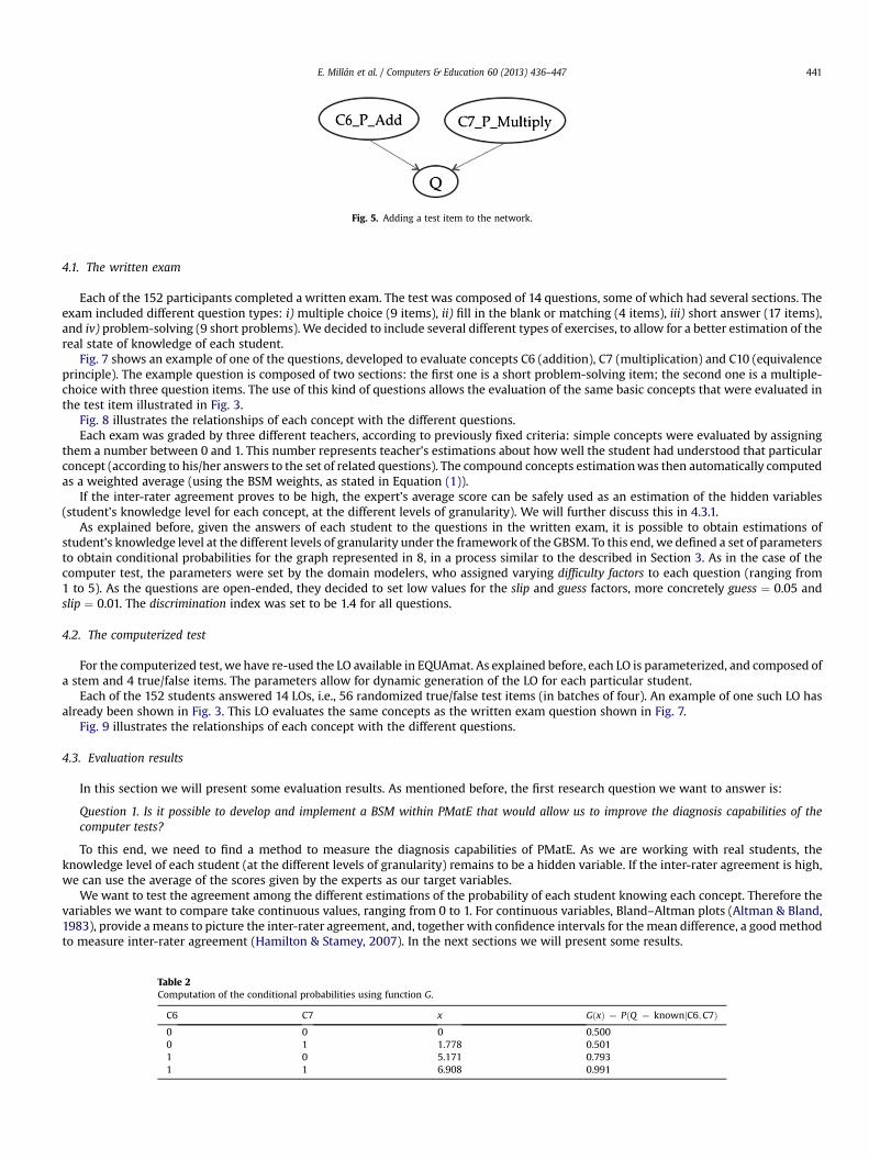
Fig. 5. Adding a test item to the network.


4.1. The written exam

Each of the 152 participants completed a written exam. The test was composed of 14 questions, some of which had several sections. Theexam included different question types: i) multiple choice (9 items), ii) fill in the blank or matching (4 items), iii) short answer (17 items),and iv) problem-solving (9 short problems). We decided to include several different types of exercises, to allow for a better estimation of thereal state of knowledge of each student.

Fig. 7 shows an example of one of the questions, developed to evaluate concepts C6 (addition), C7 (multiplication) and C10 (equivalenceprinciple). The example question is composed of two sections: the first one is a short problem-solving item; the second one is a multiple-choice with three question items. The use of this kind of questions allows the evaluation of the same basic concepts that were evaluated inthe test item illustrated in Fig. 3.

Fig. 8 illustrates the relationships of each concept with the different questions.Each exam was graded by three different teachers, according to previously fixed criteria: simple concepts were evaluated by assigning

them a number between 0 and 1. This number represents teacher’s estimations about how well the student had understood that particularconcept (according to his/her answers to the set of related questions). The compound concepts estimationwas then automatically computedas a weighted average (using the BSM weights, as stated in Equation (1)).

If the inter-rater agreement proves to be high, the expert’s average score can be safely used as an estimation of the hidden variables(student’s knowledge level for each concept, at the different levels of granularity). We will further discuss this in 4.3.1.

As explained before, given the answers of each student to the questions in the written exam, it is possible to obtain estimations ofstudent’s knowledge level at the different levels of granularity under the framework of the GBSM. To this end, we defined a set of parametersto obtain conditional probabilities for the graph represented in 8, in a process similar to the described in Section 3. As in the case of thecomputer test, the parameters were set by the domain modelers, who assigned varying difficulty factors to each question (ranging from1 to 5). As the questions are open-ended, they decided to set low values for the slip and guess factors, more concretely guess ¼ 0.05 andslip ¼ 0.01. The discrimination index was set to be 1.4 for all questions.

4.2. The computerized test

For the computerized test, we have re-used the LO available in EQUAmat. As explained before, each LO is parameterized, and composed ofa stem and 4 true/false items. The parameters allow for dynamic generation of the LO for each particular student.

Each of the 152 students answered 14 LOs, i.e., 56 randomized true/false test items (in batches of four). An example of one such LO hasalready been shown in Fig. 3. This LO evaluates the same concepts as the written exam question shown in Fig. 7.

Fig. 9 illustrates the relationships of each concept with the different questions.

4.3. Evaluation results

In this section we will present some evaluation results. As mentioned before, the first research question we want to answer is:


To this end, we need to find a method to measure the diagnosis capabilities of PMatE. As we are working with real students, theknowledge level of each student (at the different levels of granularity) remains to be a hidden variable. If the inter-rater agreement is high,we can use the average of the scores given by the experts as our target variables.

We want to test the agreement among the different estimations of the probability of each student knowing each concept. Therefore thevariables we want to compare take continuous values, ranging from 0 to 1. For continuous variables, Bland–Altman plots (Altman & Bland,1983), provide a means to picture the inter-rater agreement, and, together with confidence intervals for the mean difference, a goodmethodto measure inter-rater agreement (Hamilton & Stamey, 2007). In the next sections we will present some results.

Table 2Computation of the conditional probabilities using function G.

C6 C7 x GðxÞ ¼ PðQ ¼ knownjC6;C7Þ0 0 0 0.5000 1 1.778 0.5011 0 5.171 0.7931 1 6.908 0.991

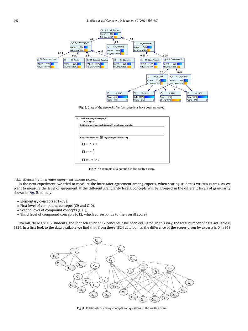
Fig. 6. State of the network after four questions have been answered.

Fig. 7. An example of a question in the written exam.


4.3.1. Measuring inter-rater agreement among expertsIn the next experiment, we tried to measure the inter-rater agreement among experts, when scoring student’s written exams. As we

want to measure the level of agreement at the different granularity levels, concepts will be grouped in the different levels of granularityshown in Fig. 6, namely:

� Elementary concepts (C1–C8),� First level of compound concepts (C9 and C10),� Second level of compound concepts (C11),� Third level of compound concepts (C12, which corresponds to the overall score).

Overall, there are 152 students, and for each student 12 concepts have been evaluated. In this way, the total number of data available is1824. In a first look to the data available we find that, from these 1824 data points, the difference of the scores given by experts is 0 in 958

Fig. 8. Relationships among concepts and questions in the written exam.

Fig. 9. Relationships among concepts and questions in the computer test.


cases (experts 1 and 2); 919 cases (experts 2 and 3) and 892 cases (experts 1 and 3). That is, the scores given by the experts are equal in78.78%, 75.58% and 73.36% of the cases, respectively.

Fig. 10 shows the Bland–Altman plots for each of these categories. Each point in the Bland–Altman plots represents one of the concepts.The x-axis value represents the average of the scores given by experts for that concept, while the y-axis represents the difference of suchscores. In this way, if both scores tend to agree, the value of y will be close to 0. Also, the lower and higher values of the abcissa representconcepts with lower and higher level of knowledge, respectively. Also, Table 3 shows the 0.05 confidence intervals for the mean difference,at each level of granularity.

The small size of the confidence intervals at the different levels of granularity shows that the inter-rater agreement is quite high. Worstresults are achieved at the second level (C11), inwhich the higher inter-rater agreement is achieved for experts 2 and 3. Bland–Altman plotsin Fig. 12 show also that the agreement is higher for students with either low or high levels of knowledge, specially in the elementary

Fig. 10. Bland–Altman plots for inter-agreement among experts.

Table 3Confidence intervals for the mean difference among experts.

Elementary (C1–C8) Mean Standard deviation Confidence intervalExpert 1 vs Expert 2 0.043 0.105 (0.037, 0.049)Expert 2 vs Expert 3 0.039 0.087 (0.034, 0.044)Expert 1 vs Expert 3 0.049 0.105 (0.044, 0.055)

First level (C9, C10) Mean Standard deviation Confidence intervalExpert 1 vs Expert 2 0.084 0.113 (0.072, 0.097)Expert 2 vs Expert 3 0.088 0.123 (0.074, 0.102)Expert 1 vs Expert 3 0.056 0.072 (0.048, 0.064)

Second level (C11) Mean Standard deviation Confidence intervalExpert 1 vs Expert 2 0.166 0.176 (0.138, 0.194)Expert 2 vs Expert 3 0.040 0.067 (0.029, 0.051)Expert 1 vs Expert 3 0.144 0.146 (0.120, 0.167)

Third level (C12) Mean Standard deviation Confidence intervalExpert 1 vs Expert 2 0.061 0.053 (0.053, 0.070)Expert 2 vs Expert 3 0.030 0.030 (0.025, 0.035)Expert 1 vs Expert 3 0.067 0.056 (0.058, 0.076)


concepts. This can be due to the fact that intermediate students are more difficult to diagnose, as their behavior when answering is moreerratic.

The small size of the confidence intervals for the mean difference allows us to conclude that the degree of agreement is quite high at thedifferent granularity levels, so we can safely use the average scores as a reasonable estimation of the student’s knowledge level.

4.3.2. Measuring inter-rater agreement among computer test, written exam, and expert averageGiven that the inter-rater agreement among experts is high, inwhat followswewill use the expert’s average score as a reliable estimation

of the student’s knowledge level at the different levels of granularity.Nowwewant tomeasure the degree of agreement among the estimations provided by the BSM defined for the computer test and also by

the estimations provided by the BSM for the written exam.Fig. 11 shows the Bland–Altman plots for the inter-rater agreement between the average of experts (Exp.Av.) and the BSM estimation

obtained for the test and also for the written exam (BN test and BN exam, respectively).

Fig. 11. Bland–Altman plots for inter-agreement among expert average, BN test and BN exam.

Fig. 12. Bland–Altman plots for BN test, Bn exam and expert average (in the overall concept C12).


Table 4 shows the 0.05 confidence intervals for the mean difference.Bland–Altman plots and confidence intervals for the mean difference help us to answer our research questions:


Question 2. Is it possible to develop and implement a BSM for the written exam that provides a reasonable estimation of the student’sknowledge level at the different levels of granularity?

Regarding the first research question, Bland–Altman plots and confidence intervals show that the answer is negative. The confidenceintervals for the mean difference account for differences between a minimum of 0.163 and a maximum of 0.337, depending on the gran-ularity level. The conclusion is that, in the current settings of PMatE, we failed to produce a BSM that would allow us to obtain a reliableestimation of student’s knowledge level at the different levels of granularity.

However, in our opinion the results have been negatively affected by a set of constraints imposed by the use of PMatE; more preciselya very high guessing factor (g¼ 0, 5) and the fact that the student needed to answer all questions even if he/shewas unsure of the right answer.These two constraints certainly increase the degree of randomness in student’s answer, thus making the diagnosis process more difficult.

With respect to the second research question, we can observe a higher degree of agreement, so the answer is positive. Both Bland–Altman plots and confidence intervals for the agreement among BSM for the written exam and expert average are very similar to thecorresponding plots and intervals for the inter-rater agreement among experts. In particular, confidence intervals show small meandifferences, comparable to the mean differences among experts, except perhaps in the case of the elementary concepts (for which theconfidence interval shows an acceptable rate of agreement) and the second level of the granularity hierarchy (where a comparabledisagreement rate among experts was also observed).

All in all, we think that the disagreement among the computer test and the expert average was due to using different instruments ofmeasure (written exam vs test) rather than to the diagnosis capabilities of the BSM.

4.3.3. Measuring inter-rater agreement among computer test with and without the BSMFinally, to answer the research question, there is still one pending issue, namely the comparison of the diagnosis capabilities of the

computer test with and without the BSM for the higher level concept or overall knowledge C12. For completeness, we will also include inthis analysis the results corresponding to the BSM over the written exam.

To this end, we assigned an overall score for each student, based on the percentage of correct answers (PCA) in the computer test, andused this measure as an estimation of the overall performance of the student in the test. This new estimation is then compared to thediagnosis obtained for the overall concept C12 for both the BSM in the computer test and the BSM in thewritten exam (BN test and BN exam,respectively), and to the expert’s average (Exp.Av.). Fig. 12 shows the corresponding Bland–Altman plots.

The 0.05 confidence intervals are shown in Table 5:

Table 4Confidence intervals for the mean difference among expert average, BN test and BN exam.

Elementary (C1–C8) Mean Standard deviation Confidence intervalExpert average vs BN test 0.317 0.223 (0.304, 0.329)Expert average vs BN exam 0.118 0.130 (0.110, 0.125)

First level (C9, C10) Mean Standard deviation Confidence IntervalExpert average vs BN test 0.255 0.175 (0.235, 0.274)Expert average vs BN exam 0.096 0.100 (0.084, 0.107)

Second level (C11) Mean Standard deviation Confidence intervalExpert average vs BN test 0.294 0.269 (0.252, 0.337)Expert average vs BN exam 0.162 0.131 (0.141, 0.183)

Third level (C12) Mean Standard deviation Confidence intervalExpert average vs BN test 0.185 0.140 (0.163, 0.208)Expert average vs BN exam 0.058 0.043 (0.051, 0.064)

Table 5Confidence intervals for the mean difference among expert’s average, BN test and BN exam, for the overall concept C12.

C12 Mean Standard deviation Confidence interval

Expert average vs BN test 0.185 0.140 (0.022, 0.163)Expert average vs BN exam 0.058 0.043 (0.007, 0.051)Expert average vs PCA 0.159 0.109 (0.017, 0.142)BN test vs PCA 0.179 0.139 (0.022, 0.160)


We can see that, compared to the expert average, PCA tends to overestimate. This is not surprising as there is a 0.5 guessing factor that hasnot been corrected. In contrast, the BN test tends to underestimate, both compared to expert average and to PCA. The performance of thecomputer test is similar in both cases (both with PCA and BSM the degree of agreement is not very high). The only case in which confidenceintervals show a high degree of agreement is for the case of BSM in the written exam and expert average. This again supports our hypothesisthat the low degree of agreement when using the computer test is due to the constraints imposed by the use of EQUAmat and not to theBSM.

5. Conclusions and future work

The work presented here can be described as the development, integration and evaluation of a Bayesian Student Model by using anexistent GBSM ((Millán & Pérez de la Cruz, 2002)) into an existing testing system (Sousa et al, 2007). To this end, the major steps have been:a) development of the Bayesian model and integration in the testing system (as described in Section 3), and b) evaluation of its diagnosiscapabilities with 152 real students.

For the evaluationwith real students, a paper and pencil test was constructed, by re-using LO in testingsystem1. Also, a written examwasdeveloped. Each of the 152 students participating in the experiment took both the computer test and the written exam. The written examwas graded by three different human experts. For comparison purposes, a BSM for the written exam has also been developed, using theGBSM approach.

The results of the evaluation have shown a high degree of inter-rater agreement among experts in the scores of the written exam, whichhas allow us to safely use the average expert’s score as a reliable estimation of student’s knowledge level at the different levels of granularity.

With respect to the diagnosis performed by the BSM of the computer tests and thewritten exam, it has been shown that the BSM definedfor the computer test fails to provide an acceptable rate of agreement with expert’s average, probably due to the restrictive conditionsimposed by the use of PMatE. However, the BSM developed for the written exam is able to provide an estimation of student’s knowledgelevel at the different levels of granularity, with a high inter-rater agreement with expert’s average (comparable to the rate of agreementamong experts). This reinforces our hypothesis that the bad results of the computer test are due to the constraints imposed by PMatE, andnot to the BSM.

Future work is planned in several different directions:

� Testing the GBSM in multiple choice tests and not forcing students to answer all questions. We think that this will reduce therandomness of the answers and facilitate a more accurate diagnosis.

� Implementation of parametric learning techniques. Though the GBSM can provide an acceptable initial BSMmodel, the use of standardparametric learning techniques can improve the quality of the parameters of the network, and therefore allowmore accurate diagnosis.

� Improvements in the theoretical model. The goal is to make the whole approach more sound and applicable to real situations. Forexample, we plan to include: questions connected to compound concepts, prerequisite relationships (Carmona, Millán, Pérez-de-la-Cruz, Trella, & Conejo, 2005, pp. 347–356) and adaptive item selection criteria (Millán & Pérez de la Cruz, 2002) that will allow toincrease the accuracy of the diagnosis while reducing the number of questions needed.

� Increased functionality. Currently, the BSM is inspectable by students. We plan to include interactivity so that for example student canselect a topic to be questioned about, and the system automatically generates the questions to be posed. In this way, whenever thestudent feels that the model does not accurately reflect his/her state of knowledge, he/she can receive a test so the model is updatedaccording to the answers given to the test.

FundingPartially supported by grant TIN2009-14179, Plan Nacional de IþDþi, Gobierno de España.

References

Altman, D. G., & Bland, J. M. (1983). Measurement in medicine: the analysis of method comparison studies. Statistician, 32, 307–317.Carmona, C., Millán, E., Pérez-de-la-Cruz, J., Trella, M., & Conejo, R. (2005). Introducing prerequisite relations in a multi-layered Bayesian student model. UM’05. LNAI 3538.

Springer Verlag.Castillo, G., Descalço, L., Diogo, S., Millán, E., Oliveira, P. & Anjo, B. (2010). Computerized Evaluation and Diagnosis of Student’s Knowledge based on Bayesian Networks. EC-TEL

2010, 5th European Conference on Technology Enhanced learning, Barcelona, LNAI 6383, 2010, (pp.494–499), Springer Verlag.Collins, J. A., Greer, J. E., & Huang, S. H. (1996). ITS’96. LNCS. Adaptive assessment using granularity hierarchies and Bayesian nets, Vol. 1086. Springer Verlag.Conati, C., Gertner, A., VanLehn, K., & Druzdzel, M. (1997). On-line student modelling for coached problem solving using Bayesian networks. In Proceedings of UM’97 (pp. 231–

242). Springer Verlag.Hamilton, C., & Stamey, J. (2007). Using Bland-Altman to assess agreement between two medical devices – don’t forget the confidence intervals. Journal Clinical Monitoring

and Computing, 21, 331–333.Jameson, A. (1996). Numerical uncertainty management in user and student modeling: an overview of systems and issues. User Modeling and User-Adapted Interaction, 5,

193–251.Millán, E., Loboda, T., & Pérez-de-la-Cruz, J. L. (2010). Bayesian networks for student model engineering. Computers and Education, 55(4), 1663–1683.


Millán, E., & Pérez de la Cruz, J. L. (2002). A Bayesian diagnostic algorithm for student modeling. User Modeling and User-Adapted Interaction, 12, 281–330.Millán, E., Pérez de la Cruz, J. L., & García, F. (2003). Dynamic versus static student models based on Bayesian networks: An empirical study. KES’03. LNCS 2774. Springer Verlag.Sousa Pinto, J., Oliveira, P., Anjo, B., Vieira, S. I., Isidro, R. O., & Silva, M. H. (2007). TDmat-mathematics diagnosis evaluation test for engineering sciences students. International

Journal of Mathematical Education in Science and Technology, 38(3), 283–299.VanLehn, K., Niu, Z., Siler, S., & Gertner, A. S. (1998). ITS’98. LNCS. Student modeling from conventional test data: A Bayesian approach without priors, Vol. 1452. Springer Verlag.VanLehn, K., Ohlsson, S., & Nason, R. (1994). Applications of simulated students: an exploration. Journal of Artificial Intelligence in Education, 5(2), 135–175.Vomlel, J. (2004). Bayesian networks in educational testing. International Journal of Uncertainty, Fuzziness and Knowledge-Based Systems, 12(Suppl. 1), 83–100.

using bayesian networks to improve knowledge assessment

Documents