users manual for an expert system … · users manual for an expert system (hspexp) for calibration...
TRANSCRIPT
USERS MANUAL FOR AN EXPERT SYSTEM (HSPEXP)FOR CALIBRATION OF THE HYDROLOGICALSIMULATION PROGRAM—FORTRAN
U.S. GEOLOGICAL SURVEYWater-Resources Investigations Report 94-4168
Users Manual for an Expert System (HSPEXP) forCalibration of the Hydrological SimulationProgram—Fortran
By Alan M. Lumb, Richard B. McCammon, and John L. Kittle, Jr.
U.S. GEOLOGICAL SURVEYWater-Resources Investigations Report 94-4168
Reston, Virginia1994
U.S. DEPARTMENT OF THE INTERIOR
BRUCE BABBITT, Secretary
U.S. GEOLOGICAL SURVEY
Gordon P. Eaton, Director
The use of trade, product, industry, or firm names is for descriptive purposes only and does not implyendorsement by the U.S. Government.
For additional information write to: Copies of this report can be purchased from:
Chief, Hydrologic Analysis Support Section U.S. Geological SurveyU.S. Geological Survey, WRD Earth Science Information Center415 National Center Open-File Reports SectionReston, VA 22092 Box 25286, MS 517
Denver Federal CenterDenver, CO 80225
CONTENTS iii
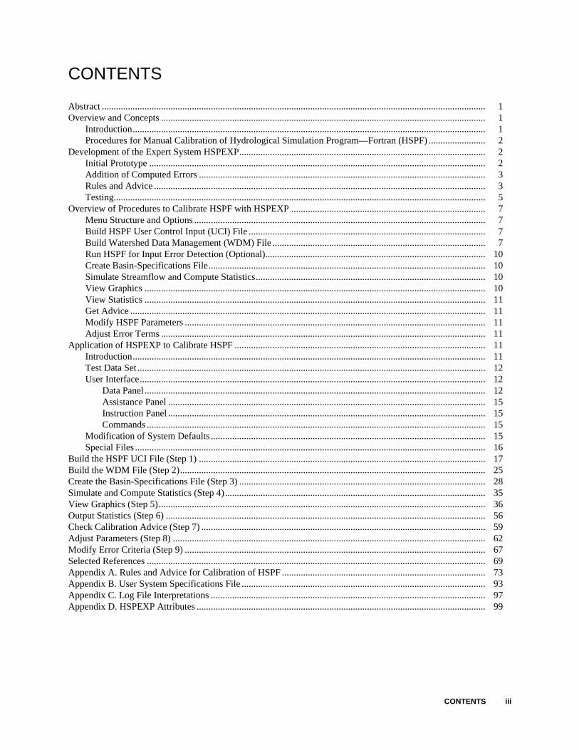
CONTENTS
Abstract .................................................................................................................................................................. 1Overview and Concepts ......................................................................................................................................... 1
Introduction..................................................................................................................................................... 1Procedures for Manual Calibration of Hydrological Simulation Program—Fortran (HSPF) ........................ 2
Development of the Expert System HSPEXP........................................................................................................ 2Initial Prototype .............................................................................................................................................. 2Addition of Computed Errors ......................................................................................................................... 3Rules and Advice ............................................................................................................................................ 3Testing............................................................................................................................................................. 5
Overview of Procedures to Calibrate HSPF with HSPEXP .................................................................................. 7Menu Structure and Options ........................................................................................................................... 7Build HSPF User Control Input (UCI) File .................................................................................................... 7Build Watershed Data Management (WDM) File .......................................................................................... 7Run HSPF for Input Error Detection (Optional)............................................................................................. 10Create Basin-Specifications File..................................................................................................................... 10Simulate Streamflow and Compute Statistics................................................................................................. 10View Graphics ................................................................................................................................................ 10View Statistics ................................................................................................................................................ 11Get Advice ...................................................................................................................................................... 11Modify HSPF Parameters ............................................................................................................................... 11Adjust Error Terms ......................................................................................................................................... 11
Application of HSPEXP to Calibrate HSPF .......................................................................................................... 11Introduction..................................................................................................................................................... 11Test Data Set ................................................................................................................................................... 12User Interface.................................................................................................................................................. 12
Data Panel................................................................................................................................................ 12Assistance Panel ...................................................................................................................................... 15Instruction Panel ...................................................................................................................................... 15Commands ............................................................................................................................................... 15
Modification of System Defaults .................................................................................................................... 15Special Files .................................................................................................................................................... 16
Build the HSPF UCI File (Step 1) ......................................................................................................................... 17Build the WDM File (Step 2)................................................................................................................................. 25Create the Basin-Specifications File (Step 3) ........................................................................................................ 28Simulate and Compute Statistics (Step 4).............................................................................................................. 35View Graphics (Step 5).......................................................................................................................................... 36Output Statistics (Step 6) ....................................................................................................................................... 56Check Calibration Advice (Step 7) ........................................................................................................................ 59Adjust Parameters (Step 8) .................................................................................................................................... 62Modify Error Criteria (Step 9) ............................................................................................................................... 67Selected References ............................................................................................................................................... 69Appendix A. Rules and Advice for Calibration of HSPF ...................................................................................... 73Appendix B. User System Specifications File ....................................................................................................... 93Appendix C. Log File Interpretations .................................................................................................................... 97Appendix D. HSPEXP Attributes .......................................................................................................................... 99
iv
FIGURES
1. General Steps for Calibrating HSPF with HSPEXP ......................................................................................... 62. Options and Menu Structure in HSPEXP, the Expert System for Calibration of HSPF .................................. 83. Detailed Steps to Calibrate HSPF with HSPEXP ............................................................................................. 94. Map of Hunting Creek, Md............................................................................................................................... 135. Basic Screen Layout and Available Commands for HSPEXP ......................................................................... 146. Listing of the UCI File for the Test Data, hunting.uci ...................................................................................... 197. Listing of Basin-Specifications File for Test Data, hunting.exs ....................................................................... 338. Time-Series Plot of Daily Precipitation and Logarithms of Daily Observed and Simulated Flow with
Flow Components ........................................................................................................................................... 429. Time-Series Plot of Daily Precipitation and Logarithms of Daily Observed and Simulated Flow .................. 4310. Time-Series Plot of Daily Precipitation and Daily Observed and Simulated Flow......................................... 4411. Time-Series Plot of Monthly Precipitation and Monthly Observed and Simulated Flow ............................... 4512. Plot of the Error in Daily Flows and the Simulated Daily Upper Zone Storage Values ................................. 4613. Plot of the Error in Daily Flows and the Simulated Daily Lower Zone Storage Values ................................. 4714. Plot of the Error in Monthly Flows and the Month of the Year....................................................................... 4815. Plot of the Error in Daily Flows and the Observed Data Flows ...................................................................... 4916. Time-Series Plot of Potential and Simulated Evapotranspiration.................................................................... 5017. Flow Duration Curves for Observed and Simulated Daily Flows ................................................................... 5118. Storm Hydrographs of Observed Flow and Simulated Flow with Flow Components .................................... 5219. Frequency Curves of Daily Computed Flow Recession Rates for Observed and Simulated Flows ............... 5320. Time-Series Plot of Cumulative Differences Between Simulated and Observed Daily Flow......................... 5421. Listing of Graphics-specifications File for Test Data, hunting.plt .................................................................. 5522. Statistics Summary of Calibration Results....................................................................................................... 56
TABLES
1. Recommended Values for TGROUP for Time Series of a Given Time Step and Record Length.................... 262. Required Data Sets for HSPEXP Applications.................................................................................................. 273. Basin-Specifications File (.exs) Content and Format ........................................................................................ 344. Graphics-Specifications File (.plt) Content and Format .................................................................................... 55B.1. TERM.DAT Parameters for General Use ...................................................................................................... 93B.2. TERM.DAT Parameters for Color Display (MS-DOS PC) ........................................................................... 93B.3. TERM.DAT Parameters for Graphics Options .............................................................................................. 94B.4. Example TERM.DAT .................................................................................................................................... 95C.1. Codes Used for Nonprinting Characters in a Log File ................................................................................... 97
CONVERSION FACTORS
Multiply By To obtain
inch (in.) 25.4 millimeter (mm)foot (ft) 0.3048 meter (m)
mile (mi) 1.609 kilometer (km)acre 0.4047 square hectometer (hm2)
acre-foot (acre-ft) 1,233 meter3 (m3)cubic foot per second (ft3/s) 0.02832 cubic meter per second (m3/s)
OVERVIEW AND CONCEPTS 1
Users Manual for an Expert System (HSPEXP) forCalibration of the Hydrological Simulation Program—Fortran
By Alan M. Lumb1, Richard B. McCammon1, and John L. Kittle, Jr.2
ABSTRACTExpert system software was developed to assist less experienced modelers with calibration of
a watershed model and to facilitate the interaction between the modeler and the modeling processnot provided by mathematical optimization. A prototype was developed with artificial intelli-gence software tools, a knowledge engineer, and two domain experts. The manual proceduresused by the domain experts were identified and the prototype was then coded by the knowledgeengineer. The expert system consists of a set of hierarchical rules designed to guide the calibrationof the model through a systematic evaluation of model parameters.
When the prototype was completed and tested, it was rewritten for portability and operationaluse and was named HSPEXP. The watershed model Hydrological Simulation Program—Fortran(HSPF) is used in the expert system. This report is the users manual for HSPEXP and contains adiscussion of the concepts and detailed steps and examples for using the software. The system hasbeen tested on watersheds in the States of Washington and Maryland, and the system correctlyidentified the model parameters to be adjusted and the adjustments led to improved calibration.
OVERVIEW AND CONCEPTS
IntroductionWatershed models have been used for more than two decades for the continuous simu-lation of river basin response to meteorologic variables of precipitation and potentialevapotranspiration for flood forecasting, stormwater management, environmentalimpact assessments, and the design and operation of water-control facilities. Variousparameters in the watershed models are modified to adapt the models to specific riverbasins. Some of the parameters can be estimated from measured properties of the riverbasins but others must be estimated by mathematical optimization or manual calibra-tion. Optimization techniques used over the past two decades have not been totally satis-factory. Such techniques reduce the interaction between the model user and themodeling process and thus do not improve user understanding of the processes as simu-lated by the model and the actual processes in the watershed. Even though objectivefunctions can be minimized by optimization, the physical meaning of such optimizedmodel parameters is left, for the most part, unexplained. Manual calibration also has not
1U.S. Geological Survey2Consultant
2 Users Manual for an Expert System (HSPEXP) for Calibration of the Hydrological Simulation Program—Fortran
been totally satisfactory because it requires experienced watershed modelers and thereare more potential users of watershed models than there are experienced modelers. Withthat in mind, the expertise of the experienced watershed modeler was placed within thecontext of an expert system so that the less-experienced modelers can “manually” cali-brate the model and improve their understanding of the link between the simulatedprocesses and the actual processes. This report describes the expert system.
The watershed model Hydrological Simulation Program—Fortran (HSPF) (Bicknelland others, 1993) was selected as the basis for testing the feasibility of developing anexpert system for parameter calibration. In earlier attempts, an expert system was devel-oped to estimate initial parameters for HSPF (Gaschnig and others, 1981). That systemweighted measured data on watershed characteristics with judgments on the importanceof the characteristic in defining the value of the parameter. Unfortunately, the softwarefor that system is not available.
Procedures for Manual Calibration of HSPFIn the present effort, two experienced watershed modelers, Alan M. Lumb andNorman H. Crawford (Hydrocomp, Inc.), documented procedures used to manuallycalibrate the rainfall-runoff module of HSPF. Richard B. McCammon was the knowl-edge engineer on the project. These calibration procedures are divided into four majorphases: (1) water balance, (2) low flow, (3) stormflow, and (4) seasonal adjustments. Afifth phase, to identify any bias within the model, was also documented. During each ofthe four major phases, a different set of calibration parameters was evaluated bycomparing simulated streamflow with observed streamflow. In more than two decadesof experience with HSPF and similar models over a wide range of climates and topog-raphies, experienced modelers have learned which parameters can be meaningfullyadjusted to reduce the error of estimation. Although the adjustments in parameter valuesduring manual calibration produce an error of estimation not significantly different frommathematical optimization routines, the parameters developed from manual calibrationcan be more meaningful and useful for regional applications of the model to ungagedwatersheds. Mathematical optimization tends to treat the model as a “black box” andusually considers minimization of only one criterion, which is typically the sum of thesquare of the difference between simulated and observed flows.
DEVELOPMENT OF THE EXPERT SYSTEM HSPEXP
Initial PrototypeFor the initial prototype of the expert system, a set of conditions was developed for eachof the major calibration phases in which the user supplies or is prompted for the generalobservations of the differences between simulated and measured flows. For example,the user would be asked if simulated stormflows are too high in the summer, if totalvolumes of simulated flow are too low, and so forth. Given the user's responses, theinitial prototype expert system identified the name of the parameter to be changed,direction of the change, and the reason for the change.
DEVELOPMENT OF THE EXPERT SYSTEM HSPEXP 3
Addition of Computed ErrorsAlthough the advice on parameter adjustments from the initial prototype of the expertsystem was useful, there was a major burden on the user as to how to identify the errorsand problems and to communicate them to the system. To ease that burden, seven errorterms are computed by the new system from the simulated and observed streamflowtime series:
1. error in total runoff volume for the calibration period,
2. error in the mean of the low-flow-recession rates based on thecomputed ratios of daily mean flow today divided by the daily mean flowyesterday for each day for the highest 30 percent (default) of the ratiosless than 1.0,
3. error in the mean of the lowest 50 percent of the daily mean flows,
4. error in the mean of the highest 10 percent of the daily mean flows,
5. error in flow volumes for selected storms,
6. seasonal volume error, June-August runoff volume error minusDecember-February runoff volume error, and
7. error in runoff volume for selected summer storms.
In addition, other computations are made:
1. ratio of simulated surface runoff and interflow volumes, and
2. the difference between the simulated actual evapotranspiration andthe potential evapotranspiration.
With these computed values, the expert system can provide advice without the subjec-tive input from the user. Several of the rules, however, contain optional subjective judg-ments that the user may supply. Examples are the type of vegetation, the water-holdingcapacity of the soil, the soil depth, or whether there is substantial recharge to a deepaquifer.
Rules and AdviceThe expert system advice is based on a set of rules that use statistical measures andsubjective judgments provided by the user that reflect the sensitivity of the parametersin the rainfall-runoff module of HSPF to those measures and judgments. The statisticalmeasures are calculated after each HSPF simulation run. The user is asked to makesubjective judgments by the prototype expert system when such judgments, in combi-nation with the rules, affect the advice offered by the program. In the final version, thesubjective judgments are optional input.
In its simplest form, a rule can be expressed by the following:
IF condition1 condition2 condition3
THEN action ,
4 Users Manual for an Expert System (HSPEXP) for Calibration of the Hydrological Simulation Program—Fortran
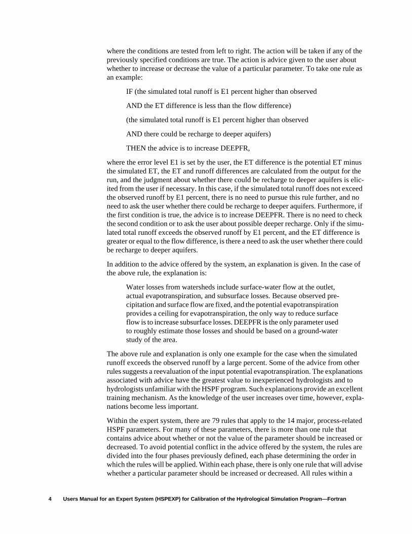
where the conditions are tested from left to right. The action will be taken if any of thepreviously specified conditions are true. The action is advice given to the user aboutwhether to increase or decrease the value of a particular parameter. To take one rule asan example:
IF (the simulated total runoff is E1 percent higher than observed
AND the ET difference is less than the flow difference)
(the simulated total runoff is E1 percent higher than observed
AND there could be recharge to deeper aquifers)
THEN the advice is to increase DEEPFR,
where the error level E1 is set by the user, the ET difference is the potential ET minusthe simulated ET, the ET and runoff differences are calculated from the output for therun, and the judgment about whether there could be recharge to deeper aquifers is elic-ited from the user if necessary. In this case, if the simulated total runoff does not exceedthe observed runoff by E1 percent, there is no need to pursue this rule further, and noneed to ask the user whether there could be recharge to deeper aquifers. Furthermore, ifthe first condition is true, the advice is to increase DEEPFR. There is no need to checkthe second condition or to ask the user about possible deeper recharge. Only if the simu-lated total runoff exceeds the observed runoff by E1 percent, and the ET difference isgreater or equal to the flow difference, is there a need to ask the user whether there couldbe recharge to deeper aquifers.
In addition to the advice offered by the system, an explanation is given. In the case ofthe above rule, the explanation is:
Water losses from watersheds include surface-water flow at the outlet,actual evapotranspiration, and subsurface losses. Because observed pre-cipitation and surface flow are fixed, and the potential evapotranspirationprovides a ceiling for evapotranspiration, the only way to reduce surfaceflow is to increase subsurface losses. DEEPFR is the only parameter usedto roughly estimate those losses and should be based on a ground-waterstudy of the area.
The above rule and explanation is only one example for the case when the simulatedrunoff exceeds the observed runoff by a large percent. Some of the advice from otherrules suggests a reevaluation of the input potential evapotranspiration. The explanationsassociated with advice have the greatest value to inexperienced hydrologists and tohydrologists unfamiliar with the HSPF program. Such explanations provide an excellenttraining mechanism. As the knowledge of the user increases over time, however, expla-nations become less important.
Within the expert system, there are 79 rules that apply to the 14 major, process-relatedHSPF parameters. For many of these parameters, there is more than one rule thatcontains advice about whether or not the value of the parameter should be increased ordecreased. To avoid potential conflict in the advice offered by the system, the rules aredivided into the four phases previously defined, each phase determining the order inwhich the rules will be applied. Within each phase, there is only one rule that will advisewhether a particular parameter should be increased or decreased. All rules within a
DEVELOPMENT OF THE EXPERT SYSTEM HSPEXP 5
phase are tested before moving on to the rules in the next phase. If any action is indicatedin testing the rules within a phase, the corresponding advice is given and no furthertesting of the rules is done. This strategy eliminates the possibility of conflicting advicebeing offered by the system.
The initial prototype is written in Envos Lisp Object-Oriented Programming System(LOOPS), formerly called Xerox LOOPS (Stefik and others, 1983). LOOPS addsaccess, object, and rule-oriented programming to the procedure-oriented programmingof Common Lisp and Interlisp-D. The result made it possible to create an extended envi-ronment for the development of the prototype. Data objects in the prototype systeminclude the main menu, the hydrologic response units, the rainfall-runoff parametersused in HSPF, the acceptable levels of error, and a number of graphical objects. On thecomputer screen, the major storm periods selected by the user are shown. The currentvalues of the acceptable level of errors can be changed at any time. Such changes maychange the states of the present rules. The icons along the bottom of the screen storeancillary information that is available to the user. Such information is the current advice,the rule descriptions, an ET map, and the storm periods currently selected. At the bottomright is the icon that, when activated, invokes execution of the HSPF program. In thisway, HSPF and the prototype are linked.
To enable distribution and provide additional testing of the expert system, the programhas been converted to American National Standards Institute (ANSI) standardlanguages using public-domain software tools for the user interface, data management,and graphics. The production version, HSPEXP, is written in Fortran with a subroutinefor each rule. The graphics utilities use the ANSI and Federal Information ProcessingStandard (FIPS) Graphical Kernel System (GKS) library, which is available for mostcomputers. The user interface uses the ANNIE Interactive Development Environment(AIDE) tool developed by the U.S. Environmental Protection Agency and the U.S.Geological Survey (Kittle and others, 1989), and a Watershed Data Management(WDM) file is used for time-series data management (Lumb and others, 1990).
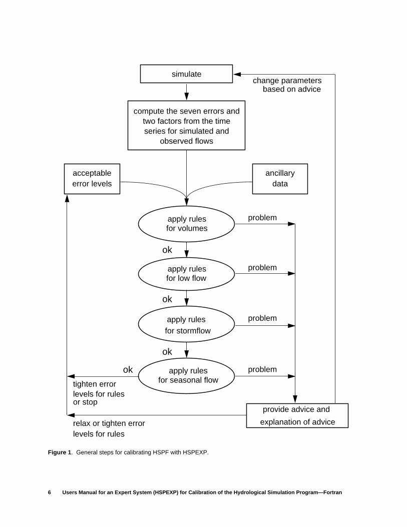
The basic steps to be followed when using HSPEXP for calibration of HSPF are shownin figure 1. HSPF may be run within HSPEXP to begin the process. HSPEXP must beused to compute the required statistics, modify acceptable levels of error, and inputancillary data. Following the advice provided by the program, HSPF parameters couldbe changed and HSPF run again or the error levels could be reset and advice requestedagain. The iterations can continue until no more advice is provided for the current errorlevels.
TestingHSPEXP has been used in the analyses of three watersheds: two rural watersheds inMaryland and an urban watershed in the Seattle, Wash., area. In each case the advicewas verified by the experienced modeler, and in each case the advice resulted in a reduc-tion of the error. Quantitative evaluations of the effectiveness of the system have not yetbeen conducted; however, the response of users in training classes has been verypositive.
6 Users Manual for an Expert System (HSPEXP) for Calibration of the Hydrological Simulation Program—Fortran
Figure 1 . General steps for calibrating HSPF with HSPEXP.
compute the seven errors andtwo factors from the timeseries for simulated and
observed flows
ancillarydata
apply rulesfor volumes
for low flow
for stormflow
for seasonal flow
provide advice and
explanation of advice
problem
problem
problem
problem
simulatechange parameters
based on advice
tighten errorlevels for rules
relax or tighten errorlevels for rules
ok
ok
ok
ok
apply rules
apply rules
apply rules
acceptableerror levels
or stop

OVERVIEW OF PROCEDURES TO CALIBRATE HSPF WITH HSPEXP 7
OVERVIEW OF PROCEDURES TO CALIBRATE HSPFWITH HSPEXP
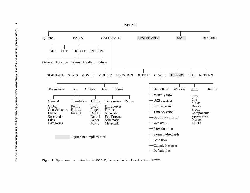
Menu Structure and OptionsThe options and menu structure for HSPEXP are shown on figure 2. The words such asBASIN and ADVISE are menu options from which the user makes a selection. Exam-ples of the menus and input forms are shown in the section “Application of HSPEXP toCalibrate HSPF.” Following any of the lowest options in the menu structure on figure2, input forms appear or an action is taken. Commands such as Help, Limits, Accept,and Previous are available in the system. Details on the use of the menus and forms arefound in the section “User Interface.”
The steps and procedures to calibrate HSPF with HSPEXP are shown in figure 3, whichexpands on figure 1. An overview of these steps is described in the following sections.
Build HSPF User Control Input (UCI) FileStep 1 is to build a UCI file within a text editor for input to HSPF, as described in theHSPF users manual (Bicknell and others, 1993) and the HSPF application guide(Donigian and others, 1984). The UCI file must have the lower case suffix .uci. Theexpert system will require some specific records on the UCI file under the EXTTARGETS block of the input. The purpose of those records is to store on the WDM filecomputed time series for eight variables used in HSPEXP in combination with observedtime series of streamflow to compute statistics needed to generate the expert advice. Theeight computed time series are:
1. simulated total runoff (inches),
2. simulated surface runoff (inches),
3. simulated interflow (inches),
4. simulated base flow (inches),
5. potential evapotranspiration (inches),
6. actual evapotranspiration (inches),
7. upper zone storage (inches), and
8. lower zone storage (inches).
If there is more than one PERLND operation or IMPLND operation, these time seriesmust be prorated by drainage area and combined before placed on the WDM file.
Build WDM FileA WDM file for the time-series input and output for HSPF must be built with theprogram ANNIE or a companion program IOWDM (Lumb and others, 1990). TheWDM file name must have the lower case suffix .wdm. The observed streamflow mustbe put in the WDM file, as well as all meteorologic time series and diversions that are
8U
sers Manual for an E
xpert System
(HS
PE
XP
) for Calibration of the H
ydrological Sim
ulation Program
—F
ortran
HSPEXP
QUERY BASIN CALIBRATE SENSITIVITY RETURN
GET PUT CREATE RETURN
SIMULATE STATS ADVISE MODIFY LOCATION OUTPUT GRAPH HISTORY
Parameters UCI Criteria Basin Return
General Simulation Utility Time series
GlobalOpn-SequenceFtableSpec-actionFiles
PerlndRchresImplnd
CopyPltgenDisplyDuranlGenerMutsin
Ext SourcesFormatsNetworkExt TargetsSchematicMass-link
Daily flow Window Edit Return
TimeSiteY-axisDevicePrecipComponentsAppearanceMarker
Monthly flow
Time vs. error
Obs flow vs. error
Weekly ET
Flow duration
Storm hydrograph
Base flow
Cumulative error
UZS vs. error
LZS vs. error
MAP
General Storms Ancillary Return
Categories
Return
PUT RETURN
Return
Default plots
- option not implemented
Figure 2 . Options and menu structure in HSPEXP, the expert system for calibration of HSPF.
Location
OVERVIEW OF PROCEDURES TO CALIBRATE HSPF WITH HSPEXP 9
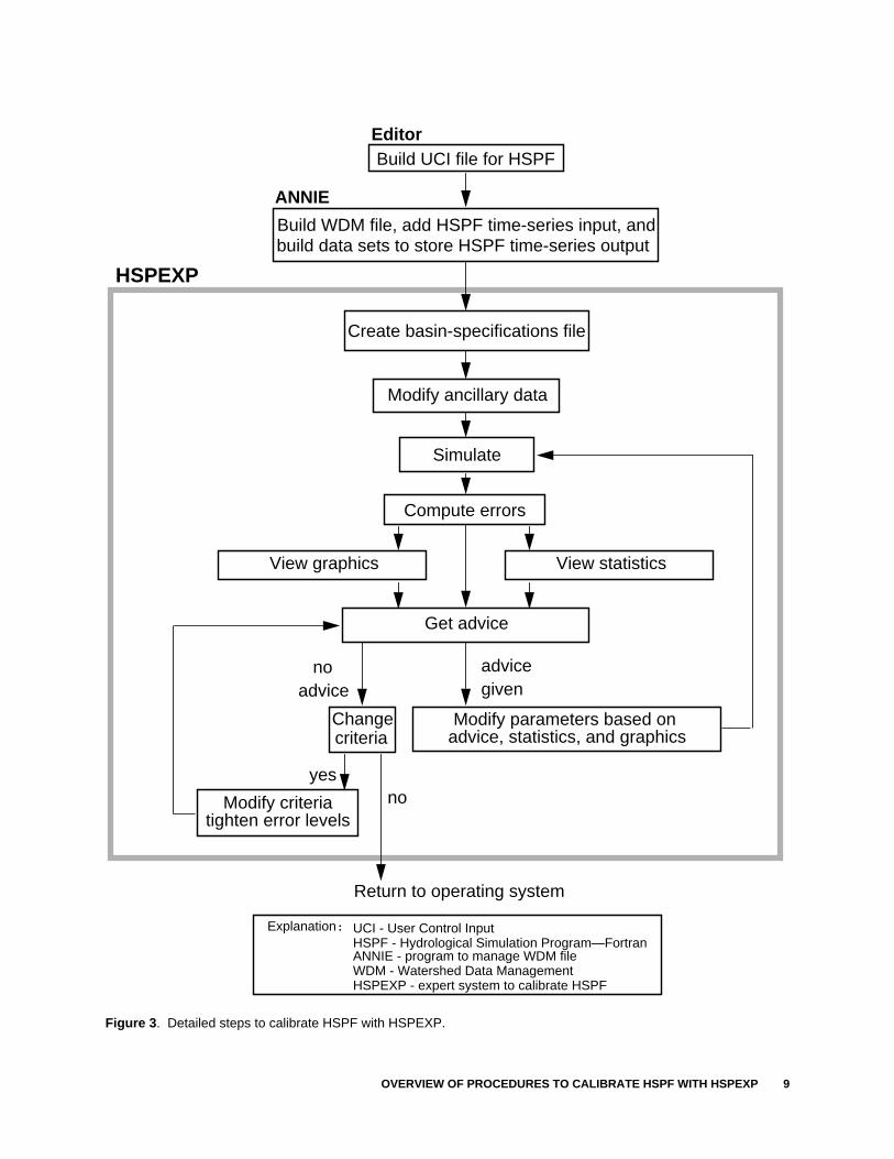
Figure 3 . Detailed steps to calibrate HSPF with HSPEXP.
Build UCI file for HSPF
Build WDM file, add HSPF time-series input, andbuild data sets to store HSPF time-series output
Simulate
advicegiven
noadvice
Modify criteria
Get advice
Modify parameters based on
Return to operating system
View graphics
HSPEXP
Editor
ANNIE
Modify ancillary data
no
Changecriteria
yes
Explanation: UCI - User Control InputHSPF - Hydrological Simulation Program—FortranANNIE - program to manage WDM file
View statistics
Compute errors
HSPEXP - expert system to calibrate HSPFWDM - Watershed Data Management
advice, statistics, and graphics
Create basin-specifications file
tighten error levels
10 Users Manual for an Expert System (HSPEXP) for Calibration of the Hydrological Simulation Program—Fortran
identified in the EXT SOURCES block of the UCI file. Data sets for storage of the nineHSPF computed time series must also be built.
Run HSPF for Input Error Detection (Optional)When the WDM and UCI files have been built, the batch version of HSPF can be run tocheck for any errors in the UCI and WDM files. HSPEXP does not provide as manychecks as the batch version of HSPF. All subsequent steps should involve runningHSPEXP.
Create Basin-Specifications FileThe acceptable limits for errors, data-set numbers for 10 of the time series, ancillarydata, storm periods, and location names are stored in a basin-specifications file. The filename must have the lower case suffix .exs. The HSPEXP CREATE option should beused to build the basin-specifications file so that the validity of the values entered ischecked.
There are 23 pieces of ancillary information that can be provided to the expert systemwith the HSPEXP CREATE menu option ANCILLARY. The defaults to each are“unknown” and will be used unless modified with HSPEXP. Rules with ancillary datawill not be used when the ancillary data values are tagged "unknown." It is useful toanswer as many of these questions as possible. To permanently store all inputs in thebasin-specifications file, the PUT option must be selected before ending an HSPEXPsession.
Simulate Streamflow and Compute StatisticsSimulate streamflow for the basin using the CALIBRATE and SIMULATE options.The expert system uses seven computed error terms along with any ancillary data tooffer advice. The error terms are computed automatically with the STATS option eachtime streamflow is simulated by using the SIMULATE option. The STATS option isincluded in the menu for the case when the HSPF simulation is done outside the expertsystem.
View GraphicsAt any time, plots can be generated to visually assess the success of the calibrations.Eleven different plots can be generated and, for UNIX workstations under X-Windows,1 to 4 of those plots can be shown on the monitor at one time. The most useful plots arethe daily and monthly flow hydrographs and the flow duration plots. The plots ofstreamflow error with upper zone storage (UZS), lower zone storage (LZS), observedflow, or time are useful at later stages of the calibration to check for various types ofbiases. The duration plot of recession rates is useful for evaluating the effectiveness ofthe recession-rate error term that is calculated and provides information to reset thecriterion that defines the percent of time that flows are in a low-flow (base flow) reces-sion period. The evapotranspiration time-series plots have less utility than the otherplots but can identify periods of moisture deficiency. The EDIT option under theGRAPH option can be selected to modify the plotting specifications. The XWINDOWoption is used to set the number of plots and their location on the monitor. When leavingthe GRAPH option, a file is written with the plotting specifications, which are applied
APPLICATION OF HSPEXP TO CALIBRATE HSPF 11
in subsequent applications of HSPEXP. The plot file has the suffix .plt and the prefixmust be the same as the .exs file.
View StatisticsThe OUTPUT option will provide the user with tables of the simulated and observedflow statistics, computed errors, and the acceptable level of errors that the expert systemuses to select which rules and advice to offer to the user. Use of the OUTPUT optioncan be helpful for statistically tracking the calibration progress and for learning param-eter sensitivity.
Get AdviceWhen the above steps have been completed, the ADVISE option in HSPEXP willprovide the user with advice on which model parameter(s) to change, the direction ofthe change, and a brief explanation. All possible advice is listed in Appendix A. Theadvice can be sent to the screen (monitor), to a file, or both.
Modify HSPF ParametersFollowing the expert system advice, an amount of change for each specified parameteris assumed. These changes are made with HSPEXP menu options CALIBRATE,MODIFY, and PARAMETERS. The UCI option can be used as a more generic alternateto the PARAMETERS option and is needed to change the multipliers in theEXTERNAL SOURCES block and to input monthly parameter values for LZETP andCEPSC. The modified parameter values will be applied for the next simulation. If apermanent change in the UCI file is desired, the BASIN and PUT options must beselected.
Adjust Error TermsInitially, the default values of the acceptable levels of error should be appropriate. Uponseveral iterations of simulation, expert advice, and parameter changes, a point may bereached where no more advice is given. At that point (1) calibration can end, (2) themodeler can make further adjustments by trial-and-error, or (3) the error terms can be“tightened.” To change (tighten or loosen) the error terms, use menu options CALI-BRATE, MODIFY, and CRITERIA. As the error terms are tightened, a point may bereached when advice will oscillate among different types of advice because no param-eter set can meet all acceptable levels of error. At this point, the calibration processshould end.
APPLICATION OF HSPEXP TO CALIBRATE HSPF
IntroductionThis section presents detailed examples illustrating the steps described in the overviewsection. Bold headings are placed at the top of each page with the title of the step foreasy reference. For each step, the procedures are described, the user interaction isshown, input or output files are listed, and output graphics are shown. The examples use
12 Users Manual for an Expert System (HSPEXP) for Calibration of the Hydrological Simulation Program—Fortran
the test data set that is distributed with the software. In addition to HSPEXP, the soft-ware packages HSPF, ANNIE, and IOWDM are needed.
Test Data SetThe test data set used for the examples is for Hunting Creek in Prince Georges County,Md. It is a small watershed of about 6,000 acres outside of Washington, D.C. The entirewatershed is located on the Geological Survey 7.5-minute series map titled PrinceFrederick Quadrangle, Maryland - Calvert County. The Geological Survey streamgage(station number 01594670) is located at the bridge on Highway 263 approximately 200feet from Highway 2. The rainfall data are from a weather station located 10 miles westin Mechanicsville, Md., and in several cases do not adequately represent the amount ofrain that fell in the watershed. The watershed is mostly forested with crop and pasturelands along the ridges. A map of the watershed is provided in figure 4.
The test data sets do not represent a final calibration. Further adjustments could be madefor a few of the parameters, additional reaches could be added, and the FTABLESrefined. Test data sets provide examples as well as data to verify that HSPEXP isinstalled correctly and reproduces the test results.
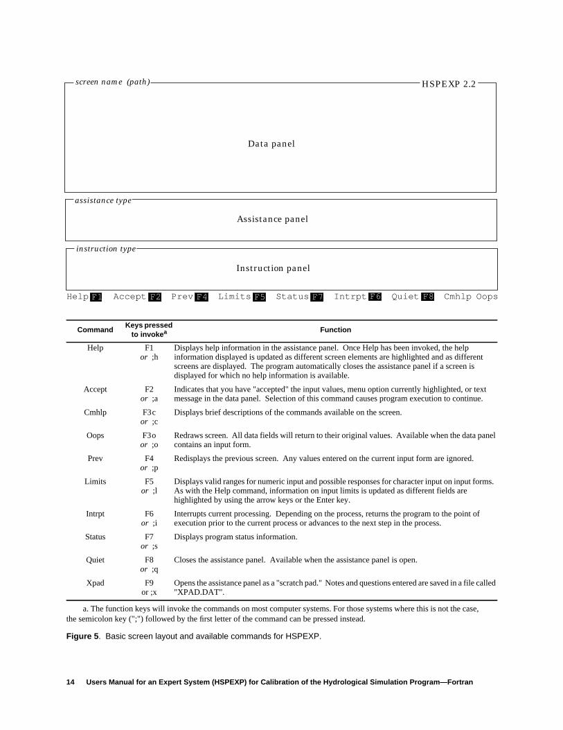
User InterfaceEach screen consists of at least two boxed-in regions or "panels," the data panel at thetop and the instruction panel at the bottom. A third region, the assistance panel, mayappear in the middle. Beneath the panels the available commands appear with their asso-ciated function keys. Commands are used to provide additional information and move-ment between screens. Figure 5 shows the basic layout of the screens. See the READMEfile distributed with the program if panel borders are not properly drawn on yourterminal.
All three panels and the line of available commands can be viewed on an 80 by 24 char-acter screen. Each panel has a distinct purpose. User interaction with the program takesplace in the data panel where menus, input forms, and informational text are displayed.In the assistance panel, help information, valid ranges for input values, and details onprogram status can be displayed. The instruction panel contains information on thekeystrokes necessary to interact with the program.
Each screen has a name, which is located where the words "screen name" appear infigure 5. The first screen is called the opening screen. All subsequent screens are givena name based on the menu option selected. Screen names are followed by a "path,"which is a list of characters representing the first letters of menu options chosen to arriveat the current screen. This list of menu initials can aid in keeping track of the position ofthe current screen in the menu hierarchy.
Data Panel
Menu options in the data panel are chosen by highlighting the desired option by usingthe arrow keys and then invoking the Accept (F2 function key) command. Alternatively,the first letter of the desired menu option can be typed. If more than one menu optionbegins with the same letter, enough characters must be typed to uniquely identify thedesired option.

APPLICATION OF HSPEXP TO CALIBRATE HSPF 13
Figure 4 . Map of Hunting Creek, Md.
14 Users Manual for an Expert System (HSPEXP) for Calibration of the Hydrological Simulation Program—Fortran
a. The function keys will invoke the commands on most computer systems. For those systems where this is not the case,the semicolon key (";") followed by the first letter of the command can be pressed instead.
Figure 5 . Basic screen layout and available commands for HSPEXP.
CommandKeys pressed
to invoke a Function
Help F1or ;h
Displays help information in the assistance panel. Once Help has been invoked, the helpinformation displayed is updated as different screen elements are highlighted and as differentscreens are displayed. The program automatically closes the assistance panel if a screen isdisplayed for which no help information is available.
Accept F2or ;a
Indicates that you have "accepted" the input values, menu option currently highlighted, or textmessage in the data panel. Selection of this command causes program execution to continue.
Cmhlp F3cor ;c
Displays brief descriptions of the commands available on the screen.
Oops F3oor ;o
Redraws screen. All data fields will return to their original values. Available when the data panelcontains an input form.
Prev F4or ;p
Redisplays the previous screen. Any values entered on the current input form are ignored.
Limits F5or ;l
Displays valid ranges for numeric input and possible responses for character input on input forms.As with the Help command, information on input limits is updated as different fields arehighlighted by using the arrow keys or the Enter key.
Intrpt F6or ;i
Interrupts current processing. Depending on the process, returns the program to the point ofexecution prior to the current process or advances to the next step in the process.
Status F7or ;s
Displays program status information.
Quiet F8or ;q
Closes the assistance panel. Available when the assistance panel is open.
Xpad F9or ;x
Opens the assistance panel as a "scratch pad." Notes and questions entered are saved in a file called"XPAD.DAT".
Help: Accept: Prev: Limits: Status: Intrpt: Quiet: Cmhlp Oops
instruction type
F1 F4
assistance type
screen name (path)
Assistance panel
Instruction panel
Data panel
F2 F5 F6 F8F7
HSPEXP 2.2

APPLICATION OF HSPEXP TO CALIBRATE HSPF 15
Input forms may require character input, such as a "yes" or "no" response, numericinput, or pressing the space bar to activate or deactivate an option. The cursor is movedaround these screens by using the arrow keys or the Enter (Return) key.
An input form may consist of a single field into which a file name is typed. These filenames are checked for validity and warnings are issued for invalid file names.
Informational text is displayed to give information on tasks in progress or alreadycompleted, as well as to give explanatory information or error messages. When thesemessages are displayed, the Accept (F2) command is invoked to continue.
Assistance Panel
The assistance panel appears when the commands Help (F1), Limits (F5), Status (F7),or Cmhlp (F3c) are invoked. The name of the command invoked appears in the upperleft corner of the assistance panel, where the words "assistance type" appear in figure 5.The assistance panel is closed by invoking the Quiet (F8) command.
In some instances, there may be more assistance information than will fit in the fouravailable lines. In these cases, the Page Up and Page Down keys can be used to scrollthrough the information, and then F3 or ";" is used to reactivate the data panel.
Instruction Panel
The instruction panel explains how to interact with the current data panel—how to enterresponses and advance to another screen. Error messages related to invalid keystrokesare also displayed in the instruction panel. When error messages are displayed, theinstruction type in the upper left corner of the panel changes from the usual"INSTRUCT" to "ERROR."
Commands
Figure 5 describes the available commands. Most commands are invoked by pressing asingle function key. The Accept (F2) command is the most frequently used command.Commands not invoked by a single function key are invoked by pressing the F3 functionkey or the semicolon key (";") followed by the first letter of the command. Pressingeither the F3 function key or the semicolon key causes the cursor to move to the bottomof the screen; any command can then be invoked by typing its first letter. Pressing eitherof these keys (F3 or ";") a second time without invoking a command will reactivate thedata panel. The F3 function key or the semicolon key is also used to reactivate the datapanel when the assistance panel becomes the active panel on the screen as describedunder "Assistance Panel."
Modification of System DefaultsWhen the program is started, the following message usually appears, "OptionalTERM.DAT file not opened, defaults will be used." System defaults have beenpredefined to suit most users’ needs, but various aspects of program operation may bemodified by creating a "TERM.DAT" file. This file resides in the directory where theprogram is being used. The format and contents of the TERM.DAT file are described inAppendix B.
16 Users Manual for an Expert System (HSPEXP) for Calibration of the Hydrological Simulation Program—Fortran
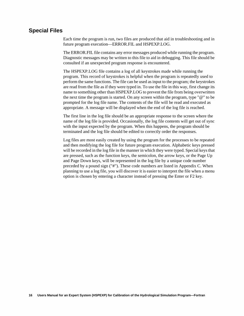
Special FilesEach time the program is run, two files are produced that aid in troubleshooting and infuture program execution—ERROR.FIL and HSPEXP.LOG.
The ERROR.FIL file contains any error messages produced while running the program.Diagnostic messages may be written to this file to aid in debugging. This file should beconsulted if an unexpected program response is encountered.
The HSPEXP.LOG file contains a log of all keystrokes made while running theprogram. This record of keystrokes is helpful when the program is repeatedly used toperform the same functions. The file can be used as input to the program; the keystrokesare read from the file as if they were typed in. To use the file in this way, first change itsname to something other than HSPEXP.LOG to prevent the file from being overwrittenthe next time the program is started. On any screen within the program, type "@" to beprompted for the log file name. The contents of the file will be read and executed asappropriate. A message will be displayed when the end of the log file is reached.
The first line in the log file should be an appropriate response to the screen where thename of the log file is provided. Occasionally, the log file contents will get out of syncwith the input expected by the program. When this happens, the program should beterminated and the log file should be edited to correctly order the responses.
Log files are most easily created by using the program for the processes to be repeatedand then modifying the log file for future program execution. Alphabetic keys pressedwill be recorded in the log file in the manner in which they were typed. Special keys thatare pressed, such as the function keys, the semicolon, the arrow keys, or the Page Upand Page Down keys, will be represented in the log file by a unique code numberpreceded by a pound sign ("#"). These code numbers are listed in Appendix C. Whenplanning to use a log file, you will discover it is easier to interpret the file when a menuoption is chosen by entering a character instead of pressing the Enter or F2 key.
Build the HSPF UCI File (Step 1) 17
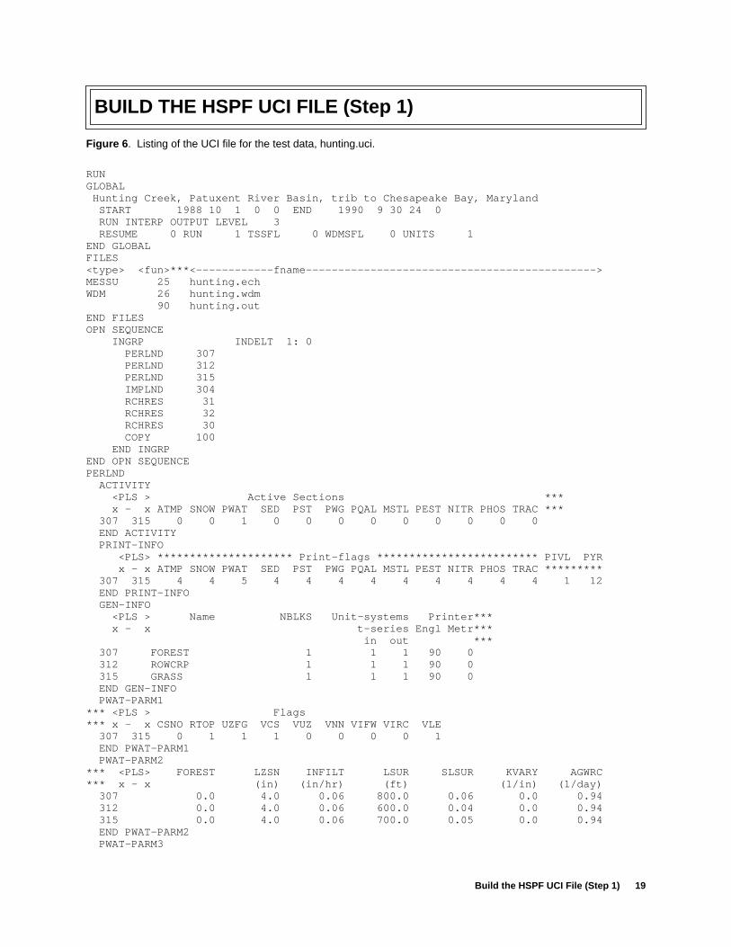
BUILD THE HSPF UCI FILE (Step 1)
To create a UCI file for your watershed or river basin, it is recommended that theUCI file listed in figure 6 for the test case be copied to your working directory.This file includes simulation of runoff and routing and does not include snowaccumulation, snowmelt, or water quality. HSPEXP can simulate snowmelt, sed-iment, and water quality, but the graphics and expert advice only apply to therunoff and routing processes. The file must be given a name followed by thesuffix .uci (for example, hunting.uci). The five files used by HSPEXP must allhave the same prefix usually taken from the name of the watershed. Suffixes forthe other four files are .wdm, .plt, .exs, and .ech; and these are described in a latersection. The HSPF users manual describing the input on the UCI file should beused along with the time-series catalog portion of the manual.
Before editing the UCI file, drainage boundaries, extent of river reaches, drain-age areas, number, location and area of PERLND and IMPLND areas, and areaof each PERLND and IMPLND by reach must be delineated and (or) determined.Automation of this process within a geographic information system (GIS) is cur-rently in a planning and design phase. The GIS would generate a file of the abovedata and the expert system would use that file to generate a UCI file.
When each of the PERLND, IMPLND, and RCHRES segments has been delin-eated, an integer number assigned, and areas tabulated, the UCI file can beedited. The editing tasks are listed below under the block headings used in theUCI file.
Modify the title line and simulation period. Column location is critical so datesand time must remain in the same columns as found in the test case UCI file.
Change the word ‘hunting’ to an identifier name for your watershed.
The time step (INDELT) is set for 1 hour in the test case UCI file. This is usuallyset at the time step of the input precipitation data, but might be increased for verylarge watersheds or decreased for very small watersheds. Change the current listof operations to include all the delineated PERLND’s, IMPLND’s, andRCHRES’s with your assigned integer number. The line with COPY mustremain so that the simulated data needed for analysis is available to the expertsystem.
For each of the PERLND’s identified in the OPN SEQUENCE block, provide thevarious tables of input options and parameters. Note the FORTRAN unit number(90 in the test case) in the GEN-INFO table must be included in the FILES block.Values in the model-parameter tables are not the best values for the test basin andare not typical or average values. If you have some experience with HSPF orHSPF has been calibrated for a watershed in the area, use this information to helpyou set initial values for the parameters. If not, read the HSPF users guide(Donigian and others, 1984) to estimate parameters or use the values in the testdata set and let the expert system provide advice on parameter-value changes.
The discussion on PERLND above also applies to the IMPLND block.
FILES
DELINEATION
GLOBAL
FILES
OPN SEQUENCE
PERLND
IMPLND
18 Users Manual for an Expert System (HSPEXP) for Calibration of the Hydrological Simulation Program—Fortran
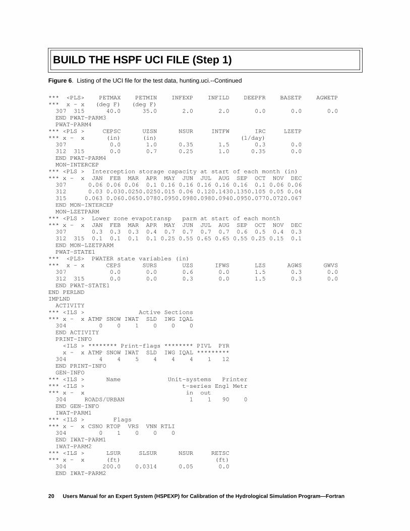
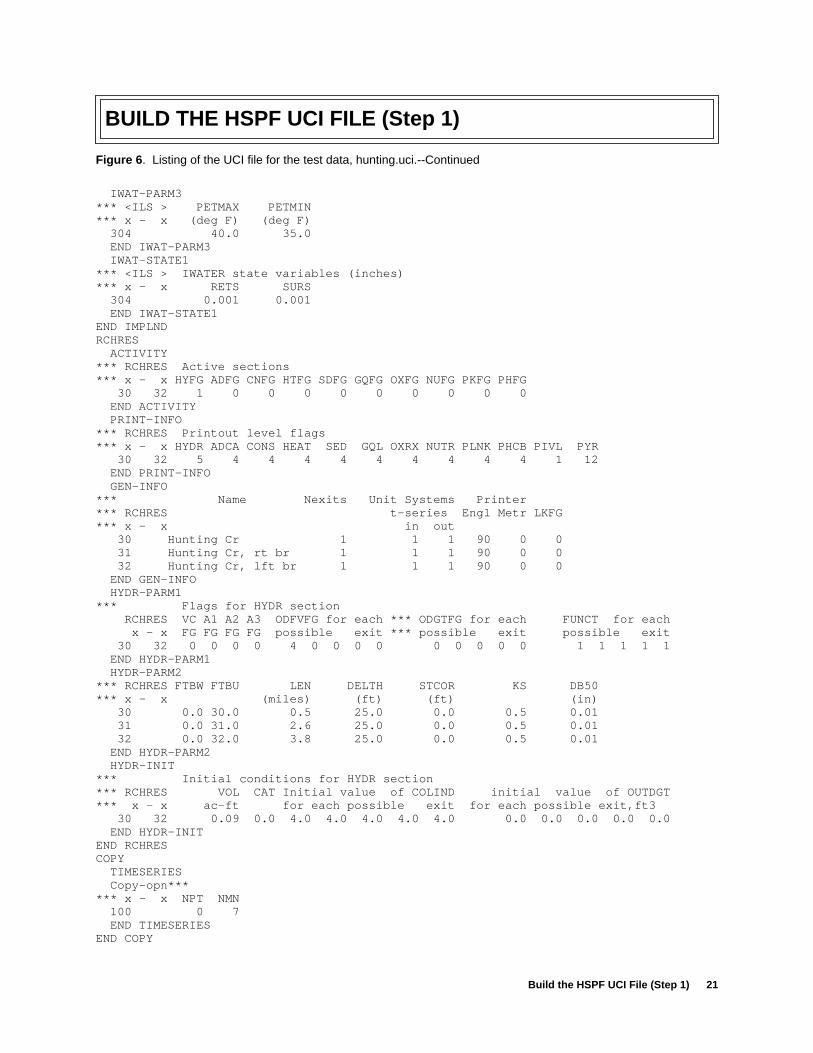
BUILD THE HSPF UCI FILE (Step 1)
Three RCHRES’s are used in the test case. Models of typical watersheds usuallyhave more RCHRES segments. As a rough rule of thumb, the average traveltimethrough a reach should very roughly approximate the time step used. Also, morethan about eight reaches above a point of interest usually does not noticeablyimprove the simulations.
The COPY block should remain and not be changed. If more output is desired,the number of time series could be increased but must not be decreased.
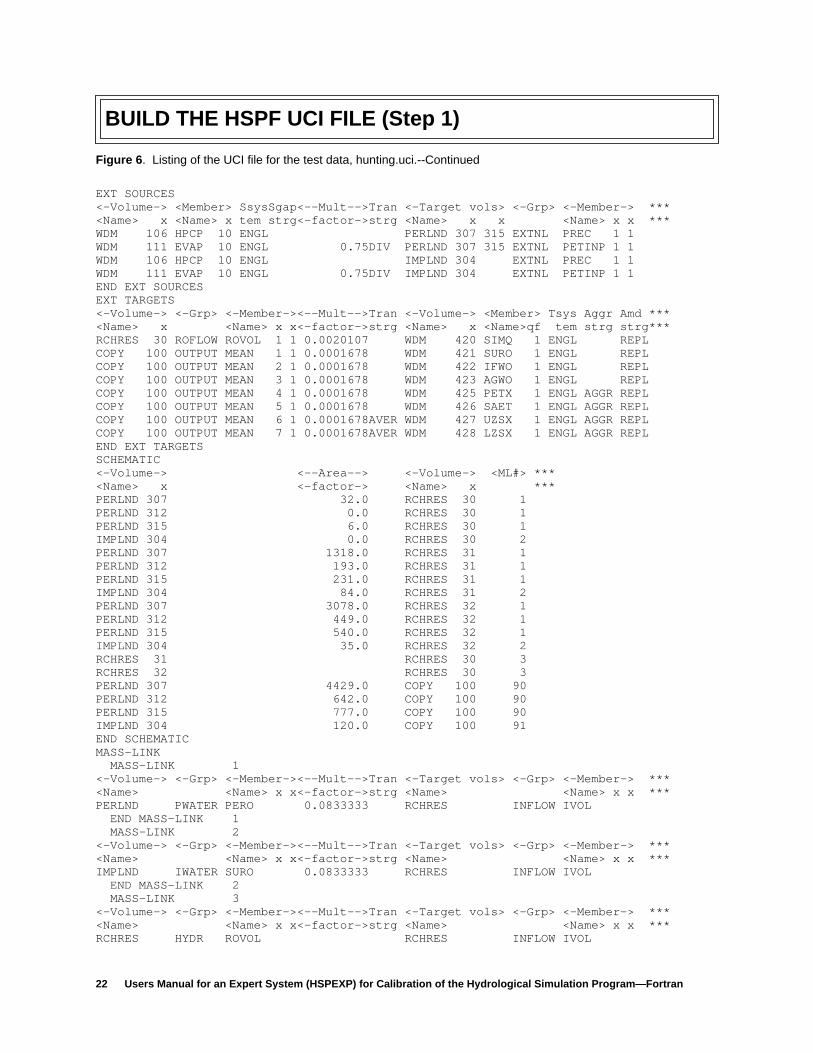
The input time series used by the expert system are identified in the EXTSOURCES block. The member names following the WDM data-set numbermust match exactly the TSTYPE name used in ANNIE or IOWDM when build-ing the WDM data sets. You will also need to enter some of these data-setnumbers when using HSPEXP to build the EXS file in step 3. A table listing allWDM data sets is provided under step 2 to assist in building the WDM data sets.
The output time series used by the expert system are identified in the EXTTARGETS block. The multiplication factor for the RCHRES item in EXTTARGETS is used to convert acre-feet/time step to watershed-inches and isequal to 12 in/ft divided by the watershed area in acres. For the PERLND items,the multiplication factor converts acre-inches to watershed-inches and is equal to1.0 divided by the watershed area in acres. The member name is the same as thetime-series types (TSTYPE) that was used when the data set was built.
The area factor (drainage area in acres) should be changed to the appropriatevalue for each PERLND and IMPLND identified in the OPN SEQUENCE block.
No changes should be made to this block.
An FTABLE must be prepared for each RCHRES specified in the RCHRESblock. An FTABLE can be used for one or more reaches if the flow characteris-tics of the reaches are similar. FTABLES can be generated from rating tableswhere streamflow is observed, can be computed from reach cross-sectional dataand Manning’s equation, or can be computed from backwater analyses withdifferent flows.
RCHRES
COPY
EXT SOURCES
EXT TARGETS
SCHEMATIC
MASS-LINK
FTABLES
Build the HSPF UCI File (Step 1) 19
BUILD THE HSPF UCI FILE (Step 1)
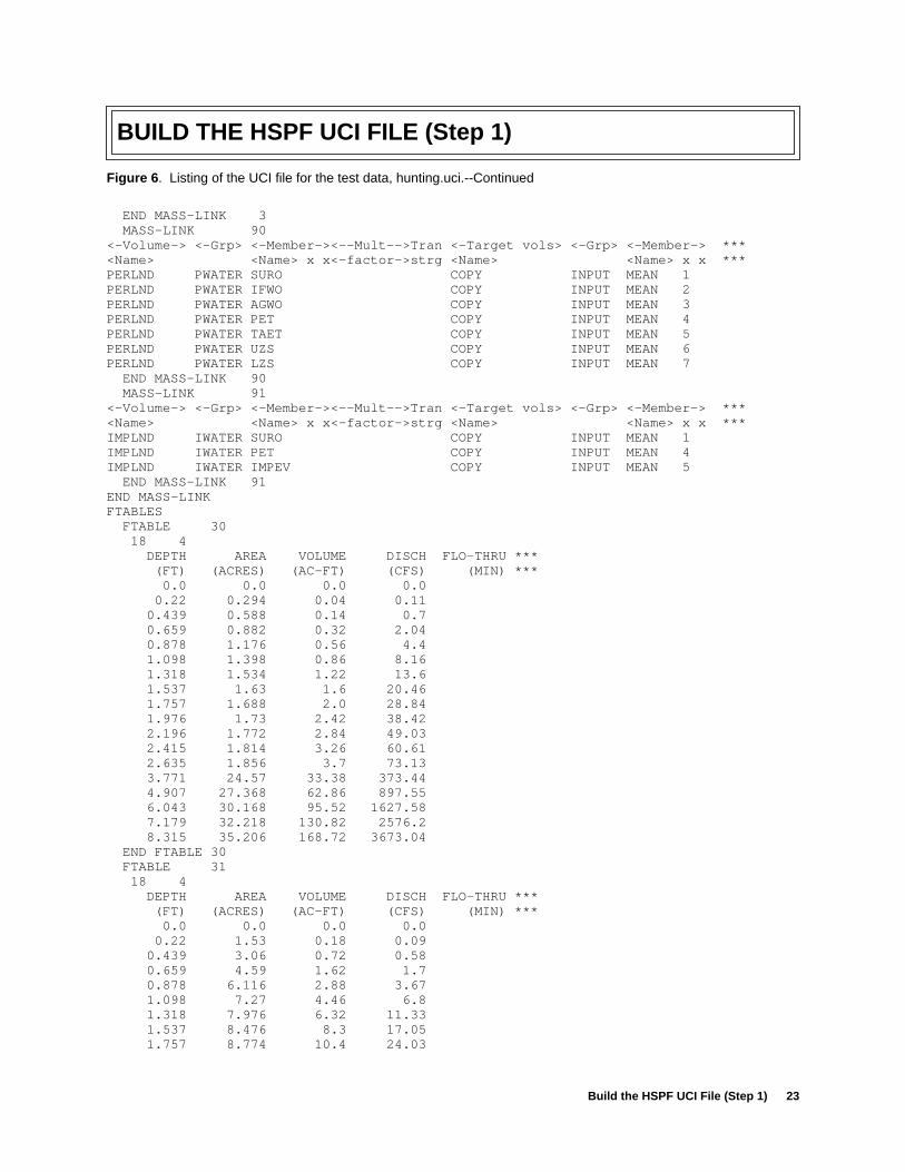
Figure 6 . Listing of the UCI file for the test data, hunting.uci.
RUNGLOBAL Hunting Creek, Patuxent River Basin, trib to Chesapeake Bay, Maryland START 1988 10 1 0 0 END 1990 9 30 24 0 RUN INTERP OUTPUT LEVEL 3 RESUME 0 RUN 1 TSSFL 0 WDMSFL 0 UNITS 1END GLOBALFILES<type> <fun>***<------------fname--------------------------------------------->MESSU 25 hunting.echWDM 26 hunting.wdm 90 hunting.outEND FILESOPN SEQUENCE INGRP INDELT 1: 0 PERLND 307 PERLND 312 PERLND 315 IMPLND 304 RCHRES 31 RCHRES 32 RCHRES 30 COPY 100 END INGRPEND OPN SEQUENCEPERLND ACTIVITY <PLS > Active Sections *** x - x ATMP SNOW PWAT SED PST PWG PQAL MSTL PEST NITR PHOS TRAC *** 307 315 0 0 1 0 0 0 0 0 0 0 0 0 END ACTIVITY PRINT-INFO <PLS> ********************* Print-flags ************************* PIVL PYR x - x ATMP SNOW PWAT SED PST PWG PQAL MSTL PEST NITR PHOS TRAC ********* 307 315 4 4 5 4 4 4 4 4 4 4 4 4 1 12 END PRINT-INFO GEN-INFO <PLS > Name NBLKS Unit-systems Printer*** x - x t-series Engl Metr*** in out *** 307 FOREST 1 1 1 90 0 312 ROWCRP 1 1 1 90 0 315 GRASS 1 1 1 90 0 END GEN-INFO PWAT-PARM1*** <PLS > Flags*** x - x CSNO RTOP UZFG VCS VUZ VNN VIFW VIRC VLE 307 315 0 1 1 1 0 0 0 0 1 END PWAT-PARM1 PWAT-PARM2*** <PLS> FOREST LZSN INFILT LSUR SLSUR KVARY AGWRC*** x - x (in) (in/hr) (ft) (1/in) (1/day) 307 0.0 4.0 0.06 800.0 0.06 0.0 0.94 312 0.0 4.0 0.06 600.0 0.04 0.0 0.94 315 0.0 4.0 0.06 700.0 0.05 0.0 0.94 END PWAT-PARM2 PWAT-PARM3
20 Users Manual for an Expert System (HSPEXP) for Calibration of the Hydrological Simulation Program—Fortran
BUILD THE HSPF UCI FILE (Step 1)
Figure 6 . Listing of the UCI file for the test data, hunting.uci.--Continued
*** <PLS> PETMAX PETMIN INFEXP INFILD DEEPFR BASETP AGWETP*** x - x (deg F) (deg F) 307 315 40.0 35.0 2.0 2.0 0.0 0.0 0.0 END PWAT-PARM3 PWAT-PARM4*** <PLS > CEPSC UZSN NSUR INTFW IRC LZETP*** x - x (in) (in) (1/day) 307 0.0 1.0 0.35 1.5 0.3 0.0 312 315 0.0 0.7 0.25 1.0 0.35 0.0 END PWAT-PARM4 MON-INTERCEP*** <PLS > Interception storage capacity at start of each month (in)*** x - x JAN FEB MAR APR MAY JUN JUL AUG SEP OCT NOV DEC 307 0.06 0.06 0.06 0.1 0.16 0.16 0.16 0.16 0.16 0.1 0.06 0.06 312 0.03 0.030.0250.0250.015 0.06 0.120.1430.1350.105 0.05 0.04 315 0.063 0.060.0650.0780.0950.0980.0980.0940.0950.0770.0720.067 END MON-INTERCEP MON-LZETPARM*** <PLS > Lower zone evapotransp parm at start of each month*** x - x JAN FEB MAR APR MAY JUN JUL AUG SEP OCT NOV DEC 307 0.3 0.3 0.3 0.4 0.7 0.7 0.7 0.7 0.6 0.5 0.4 0.3 312 315 0.1 0.1 0.1 0.1 0.25 0.55 0.65 0.65 0.55 0.25 0.15 0.1 END MON-LZETPARM PWAT-STATE1*** <PLS> PWATER state variables (in)*** x - x CEPS SURS UZS IFWS LZS AGWS GWVS 307 0.0 0.0 0.6 0.0 1.5 0.3 0.0 312 315 0.0 0.0 0.3 0.0 1.5 0.3 0.0 END PWAT-STATE1END PERLNDIMPLND ACTIVITY*** <ILS > Active Sections*** x - x ATMP SNOW IWAT SLD IWG IQAL 304 0 0 1 0 0 0 END ACTIVITY PRINT-INFO <ILS > ******** Print-flags ******** PIVL PYR x - x ATMP SNOW IWAT SLD IWG IQAL ********* 304 4 4 5 4 4 4 1 12 END PRINT-INFO GEN-INFO*** <ILS > Name Unit-systems Printer*** <ILS > t-series Engl Metr*** x - x in out 304 ROADS/URBAN 1 1 90 0 END GEN-INFO IWAT-PARM1*** <ILS > Flags*** x - x CSNO RTOP VRS VNN RTLI 304 0 1 0 0 0 END IWAT-PARM1 IWAT-PARM2*** <ILS > LSUR SLSUR NSUR RETSC*** x - x (ft) (ft) 304 200.0 0.0314 0.05 0.0 END IWAT-PARM2
Build the HSPF UCI File (Step 1) 21
BUILD THE HSPF UCI FILE (Step 1)
Figure 6 . Listing of the UCI file for the test data, hunting.uci.--Continued
IWAT-PARM3*** <ILS > PETMAX PETMIN*** x - x (deg F) (deg F) 304 40.0 35.0 END IWAT-PARM3 IWAT-STATE1*** <ILS > IWATER state variables (inches)*** x - x RETS SURS 304 0.001 0.001 END IWAT-STATE1END IMPLNDRCHRES ACTIVITY*** RCHRES Active sections*** x - x HYFG ADFG CNFG HTFG SDFG GQFG OXFG NUFG PKFG PHFG 30 32 1 0 0 0 0 0 0 0 0 0 END ACTIVITY PRINT-INFO*** RCHRES Printout level flags*** x - x HYDR ADCA CONS HEAT SED GQL OXRX NUTR PLNK PHCB PIVL PYR 30 32 5 4 4 4 4 4 4 4 4 4 1 12 END PRINT-INFO GEN-INFO*** Name Nexits Unit Systems Printer*** RCHRES t-series Engl Metr LKFG*** x - x in out 30 Hunting Cr 1 1 1 90 0 0 31 Hunting Cr, rt br 1 1 1 90 0 0 32 Hunting Cr, lft br 1 1 1 90 0 0 END GEN-INFO HYDR-PARM1*** Flags for HYDR section RCHRES VC A1 A2 A3 ODFVFG for each *** ODGTFG for each FUNCT for each x - x FG FG FG FG possible exit *** possible exit possible exit 30 32 0 0 0 0 4 0 0 0 0 0 0 0 0 0 1 1 1 1 1 END HYDR-PARM1 HYDR-PARM2*** RCHRES FTBW FTBU LEN DELTH STCOR KS DB50*** x - x (miles) (ft) (ft) (in) 30 0.0 30.0 0.5 25.0 0.0 0.5 0.01 31 0.0 31.0 2.6 25.0 0.0 0.5 0.01 32 0.0 32.0 3.8 25.0 0.0 0.5 0.01 END HYDR-PARM2 HYDR-INIT*** Initial conditions for HYDR section*** RCHRES VOL CAT Initial value of COLIND initial value of OUTDGT*** x - x ac-ft for each possible exit for each possible exit,ft3 30 32 0.09 0.0 4.0 4.0 4.0 4.0 4.0 0.0 0.0 0.0 0.0 0.0 END HYDR-INITEND RCHRESCOPY TIMESERIES Copy-opn****** x - x NPT NMN 100 0 7 END TIMESERIESEND COPY
22 Users Manual for an Expert System (HSPEXP) for Calibration of the Hydrological Simulation Program—Fortran
BUILD THE HSPF UCI FILE (Step 1)
Figure 6 . Listing of the UCI file for the test data, hunting.uci.--Continued
EXT SOURCES<-Volume-> <Member> SsysSgap<--Mult-->Tran <-Target vols> <-Grp> <-Member-> ***<Name> x <Name> x tem strg<-factor->strg <Name> x x <Name> x x ***WDM 106 HPCP 10 ENGL PERLND 307 315 EXTNL PREC 1 1WDM 111 EVAP 10 ENGL 0.75DIV PERLND 307 315 EXTNL PETINP 1 1WDM 106 HPCP 10 ENGL IMPLND 304 EXTNL PREC 1 1WDM 111 EVAP 10 ENGL 0.75DIV IMPLND 304 EXTNL PETINP 1 1END EXT SOURCESEXT TARGETS<-Volume-> <-Grp> <-Member-><--Mult-->Tran <-Volume-> <Member> Tsys Aggr Amd ***<Name> x <Name> x x<-factor->strg <Name> x <Name>qf tem strg strg***RCHRES 30 ROFLOW ROVOL 1 1 0.0020107 WDM 420 SIMQ 1 ENGL REPLCOPY 100 OUTPUT MEAN 1 1 0.0001678 WDM 421 SURO 1 ENGL REPLCOPY 100 OUTPUT MEAN 2 1 0.0001678 WDM 422 IFWO 1 ENGL REPLCOPY 100 OUTPUT MEAN 3 1 0.0001678 WDM 423 AGWO 1 ENGL REPLCOPY 100 OUTPUT MEAN 4 1 0.0001678 WDM 425 PETX 1 ENGL AGGR REPLCOPY 100 OUTPUT MEAN 5 1 0.0001678 WDM 426 SAET 1 ENGL AGGR REPLCOPY 100 OUTPUT MEAN 6 1 0.0001678AVER WDM 427 UZSX 1 ENGL AGGR REPLCOPY 100 OUTPUT MEAN 7 1 0.0001678AVER WDM 428 LZSX 1 ENGL AGGR REPLEND EXT TARGETSSCHEMATIC<-Volume-> <--Area--> <-Volume-> <ML#> ***<Name> x <-factor-> <Name> x ***PERLND 307 32.0 RCHRES 30 1PERLND 312 0.0 RCHRES 30 1PERLND 315 6.0 RCHRES 30 1IMPLND 304 0.0 RCHRES 30 2PERLND 307 1318.0 RCHRES 31 1PERLND 312 193.0 RCHRES 31 1PERLND 315 231.0 RCHRES 31 1IMPLND 304 84.0 RCHRES 31 2PERLND 307 3078.0 RCHRES 32 1PERLND 312 449.0 RCHRES 32 1PERLND 315 540.0 RCHRES 32 1IMPLND 304 35.0 RCHRES 32 2RCHRES 31 RCHRES 30 3RCHRES 32 RCHRES 30 3PERLND 307 4429.0 COPY 100 90PERLND 312 642.0 COPY 100 90PERLND 315 777.0 COPY 100 90IMPLND 304 120.0 COPY 100 91END SCHEMATICMASS-LINK MASS-LINK 1<-Volume-> <-Grp> <-Member-><--Mult-->Tran <-Target vols> <-Grp> <-Member-> ***<Name> <Name> x x<-factor->strg <Name> <Name> x x ***PERLND PWATER PERO 0.0833333 RCHRES INFLOW IVOL END MASS-LINK 1 MASS-LINK 2<-Volume-> <-Grp> <-Member-><--Mult-->Tran <-Target vols> <-Grp> <-Member-> ***<Name> <Name> x x<-factor->strg <Name> <Name> x x ***IMPLND IWATER SURO 0.0833333 RCHRES INFLOW IVOL END MASS-LINK 2 MASS-LINK 3<-Volume-> <-Grp> <-Member-><--Mult-->Tran <-Target vols> <-Grp> <-Member-> ***<Name> <Name> x x<-factor->strg <Name> <Name> x x ***RCHRES HYDR ROVOL RCHRES INFLOW IVOL
Build the HSPF UCI File (Step 1) 23
BUILD THE HSPF UCI FILE (Step 1)
Figure 6 . Listing of the UCI file for the test data, hunting.uci.--Continued
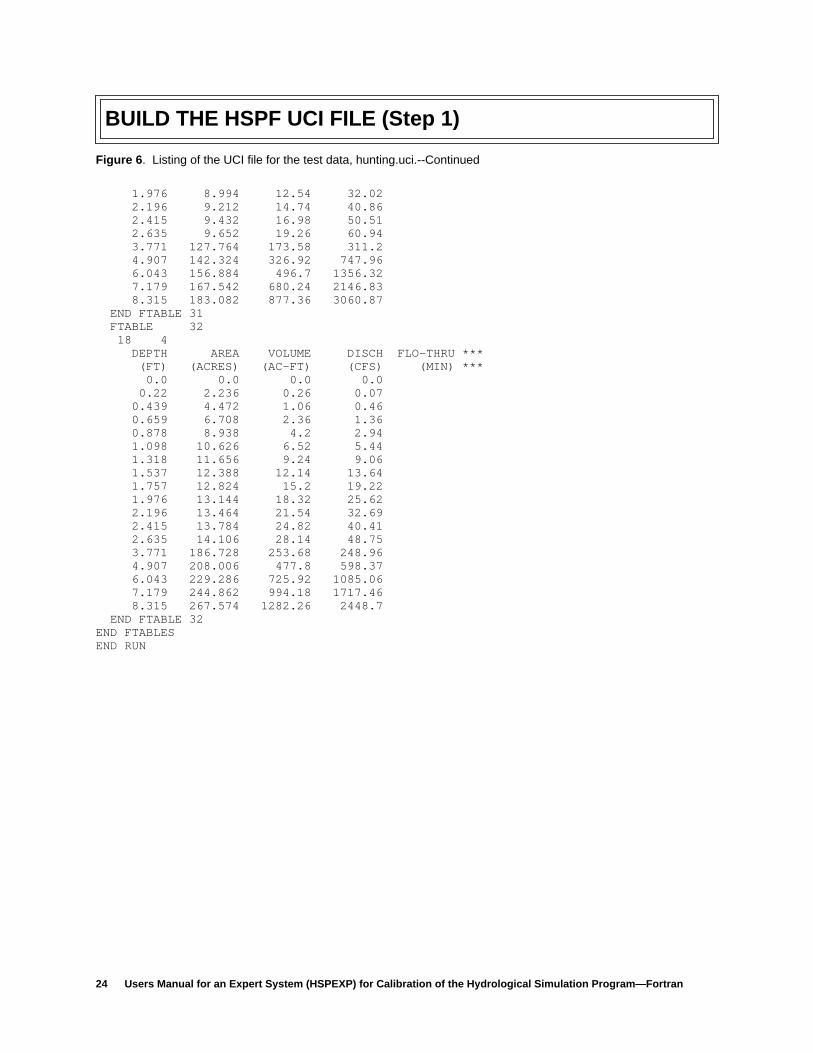
END MASS-LINK 3 MASS-LINK 90<-Volume-> <-Grp> <-Member-><--Mult-->Tran <-Target vols> <-Grp> <-Member-> ***<Name> <Name> x x<-factor->strg <Name> <Name> x x ***PERLND PWATER SURO COPY INPUT MEAN 1PERLND PWATER IFWO COPY INPUT MEAN 2PERLND PWATER AGWO COPY INPUT MEAN 3PERLND PWATER PET COPY INPUT MEAN 4PERLND PWATER TAET COPY INPUT MEAN 5PERLND PWATER UZS COPY INPUT MEAN 6PERLND PWATER LZS COPY INPUT MEAN 7 END MASS-LINK 90 MASS-LINK 91<-Volume-> <-Grp> <-Member-><--Mult-->Tran <-Target vols> <-Grp> <-Member-> ***<Name> <Name> x x<-factor->strg <Name> <Name> x x ***IMPLND IWATER SURO COPY INPUT MEAN 1IMPLND IWATER PET COPY INPUT MEAN 4IMPLND IWATER IMPEV COPY INPUT MEAN 5 END MASS-LINK 91END MASS-LINKFTABLES FTABLE 30 18 4 DEPTH AREA VOLUME DISCH FLO-THRU *** (FT) (ACRES) (AC-FT) (CFS) (MIN) *** 0.0 0.0 0.0 0.0 0.22 0.294 0.04 0.11 0.439 0.588 0.14 0.7 0.659 0.882 0.32 2.04 0.878 1.176 0.56 4.4 1.098 1.398 0.86 8.16 1.318 1.534 1.22 13.6 1.537 1.63 1.6 20.46 1.757 1.688 2.0 28.84 1.976 1.73 2.42 38.42 2.196 1.772 2.84 49.03 2.415 1.814 3.26 60.61 2.635 1.856 3.7 73.13 3.771 24.57 33.38 373.44 4.907 27.368 62.86 897.55 6.043 30.168 95.52 1627.58 7.179 32.218 130.82 2576.2 8.315 35.206 168.72 3673.04 END FTABLE 30 FTABLE 31 18 4 DEPTH AREA VOLUME DISCH FLO-THRU *** (FT) (ACRES) (AC-FT) (CFS) (MIN) *** 0.0 0.0 0.0 0.0 0.22 1.53 0.18 0.09 0.439 3.06 0.72 0.58 0.659 4.59 1.62 1.7 0.878 6.116 2.88 3.67 1.098 7.27 4.46 6.8 1.318 7.976 6.32 11.33 1.537 8.476 8.3 17.05 1.757 8.774 10.4 24.03
24 Users Manual for an Expert System (HSPEXP) for Calibration of the Hydrological Simulation Program—Fortran
BUILD THE HSPF UCI FILE (Step 1)
Figure 6 . Listing of the UCI file for the test data, hunting.uci.--Continued
1.976 8.994 12.54 32.02 2.196 9.212 14.74 40.86 2.415 9.432 16.98 50.51 2.635 9.652 19.26 60.94 3.771 127.764 173.58 311.2 4.907 142.324 326.92 747.96 6.043 156.884 496.7 1356.32 7.179 167.542 680.24 2146.83 8.315 183.082 877.36 3060.87 END FTABLE 31 FTABLE 32 18 4 DEPTH AREA VOLUME DISCH FLO-THRU *** (FT) (ACRES) (AC-FT) (CFS) (MIN) *** 0.0 0.0 0.0 0.0 0.22 2.236 0.26 0.07 0.439 4.472 1.06 0.46 0.659 6.708 2.36 1.36 0.878 8.938 4.2 2.94 1.098 10.626 6.52 5.44 1.318 11.656 9.24 9.06 1.537 12.388 12.14 13.64 1.757 12.824 15.2 19.22 1.976 13.144 18.32 25.62 2.196 13.464 21.54 32.69 2.415 13.784 24.82 40.41 2.635 14.106 28.14 48.75 3.771 186.728 253.68 248.96 4.907 208.006 477.8 598.37 6.043 229.286 725.92 1085.06 7.179 244.862 994.18 1717.46 8.315 267.574 1282.26 2448.7 END FTABLE 32END FTABLESEND RUN

Build the WDM File (Step 2) 25
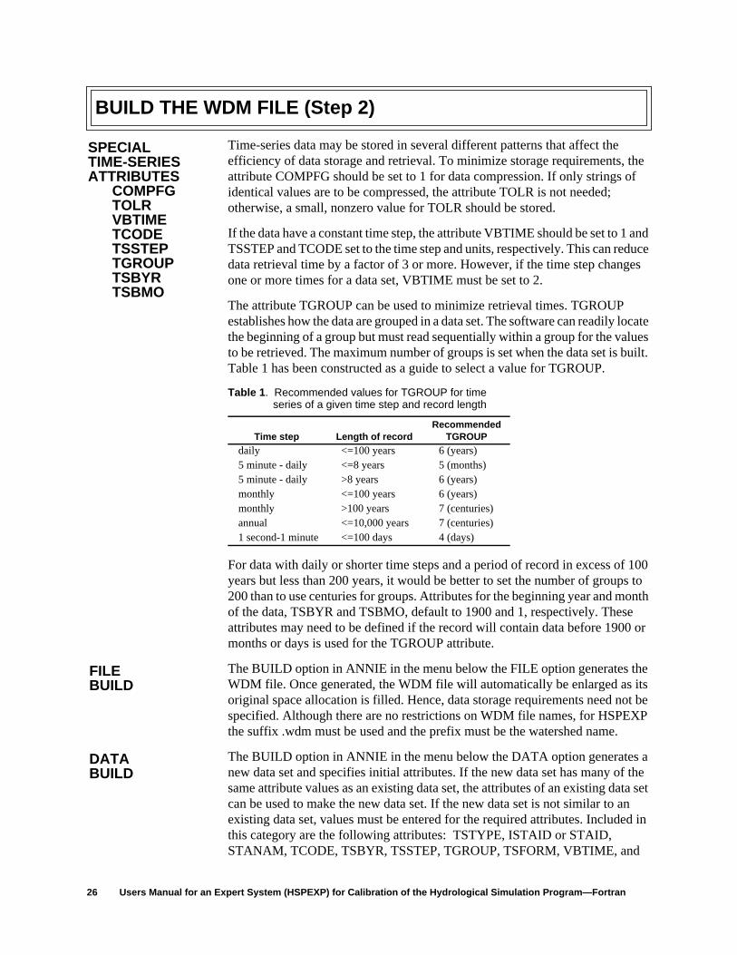
BUILD THE WDM FILE (Step 2)
The program ANNIE is used for this step. After the WDM file has been built, allthe WDM data sets identified in the UCI file from step 1 must be added. For thedata sets in the EXT SOURCES block of the UCI file, the meteorologic timeseries must be added to the data set using the ANNIE IMPORT option or theprogram IOWDM. A general discussion of the WDM file follows and is verysimilar to the same discussion found in the ANNIE users manual (Lumb andothers, 1990).
The WDM file is a binary, direct-access file used to store hydrologic, hydraulic,meteorologic, water-quality, and physiographic data. The WDM file is organizedinto data sets. Each data set contains a specific type of data, such as streamflowat a specific site or air temperature at a weather station. Each data set containsattributes that describe the data, such as station identification number, time stepof data, latitude, and longitude. The WDM file can contain up to 32,000 data sets.Each data set may be described by either a few attributes or by hundreds ofattributes. The WDM file may contain data for all data-collection stations for abasin, for a State, or for any other grouping selected by the user.
Disk space for the WDM file is allocated as needed in 40,960-byte increments(20 2,048-byte records). Data can be added, deleted, and modified withoutrestructuring the data in the file. Space from deleted data sets within a WDM fileis reused. Thus, the WDM file requires no special maintenance processing.
Time-series data can have time steps from 1 second to 1 year and can be groupedin periods of 1 hour to 1 century. Data are grouped for rapid access. Data may betagged with a quality flag to indicate missing records, estimated data, historicfloods, and so forth.
Time-series data are stored in a data set in one of two forms: compressed oruncompressed. The compressed form stores a value for every time step onlywhen adjacent values are not the same or differ by more than a preset tolerance(see attribute TOLR). The uncompressed form stores a value for every time step.For adjacent values that are the same or less than the tolerance, the value and thenumber of time steps with that value are stored.
Before data are added to a WDM file, a unique data-set number (DSN) andvalues for required attributes that describe how the data are stored must beassigned. Once data have been added, the required attributes can no longer bemodified. An extensive list of optional attributes is available for furthercharacterization of data contained in a WDM data set. The current list of requiredand optional data-set attributes is provided in Appendix D. Optional attributescan be added to a data set at any time, but it is good practice to add them whenthe data set is prepared.
WDM FILE
STRUCTURE andMAINTENANCE
TIME-SERIESDATA SETS
TIME-SERIESDATACOMPRESSION
DATA-SETATTRIBUTES
26 Users Manual for an Expert System (HSPEXP) for Calibration of the Hydrological Simulation Program—Fortran
BUILD THE WDM FILE (Step 2)
Time-series data may be stored in several different patterns that affect theefficiency of data storage and retrieval. To minimize storage requirements, theattribute COMPFG should be set to 1 for data compression. If only strings ofidentical values are to be compressed, the attribute TOLR is not needed;otherwise, a small, nonzero value for TOLR should be stored.
If the data have a constant time step, the attribute VBTIME should be set to 1 andTSSTEP and TCODE set to the time step and units, respectively. This can reducedata retrieval time by a factor of 3 or more. However, if the time step changesone or more times for a data set, VBTIME must be set to 2.
The attribute TGROUP can be used to minimize retrieval times. TGROUPestablishes how the data are grouped in a data set. The software can readily locatethe beginning of a group but must read sequentially within a group for the valuesto be retrieved. The maximum number of groups is set when the data set is built.Table 1 has been constructed as a guide to select a value for TGROUP.
For data with daily or shorter time steps and a period of record in excess of 100years but less than 200 years, it would be better to set the number of groups to200 than to use centuries for groups. Attributes for the beginning year and monthof the data, TSBYR and TSBMO, default to 1900 and 1, respectively. Theseattributes may need to be defined if the record will contain data before 1900 ormonths or days is used for the TGROUP attribute.
The BUILD option in ANNIE in the menu below the FILE option generates theWDM file. Once generated, the WDM file will automatically be enlarged as itsoriginal space allocation is filled. Hence, data storage requirements need not bespecified. Although there are no restrictions on WDM file names, for HSPEXPthe suffix .wdm must be used and the prefix must be the watershed name.
The BUILD option in ANNIE in the menu below the DATA option generates anew data set and specifies initial attributes. If the new data set has many of thesame attribute values as an existing data set, the attributes of an existing data setcan be used to make the new data set. If the new data set is not similar to anexisting data set, values must be entered for the required attributes. Included inthis category are the following attributes: TSTYPE, ISTAID or STAID,STANAM, TCODE, TSBYR, TSSTEP, TGROUP, TSFORM, VBTIME, and
Table 1 . Recommended values for TGROUP for timeseries of a given time step and record length
Time step Length of recordRecommended
TGROUPdaily <=100 years 6 (years)5 minute - daily <=8 years 5 (months)5 minute - daily >8 years 6 (years)monthly <=100 years 6 (years)monthly >100 years 7 (centuries)annual <=10,000 years 7 (centuries)1 second-1 minute <=100 days 4 (days)
SPECIALTIME-SERIESATTRIBUTES
COMPFGTOLRVBTIMETCODETSSTEPTGROUPTSBYRTSBMO
FILEBUILD
DATABUILD
Build the WDM File (Step 2) 27
BUILD THE WDM FILE (Step 2)
COMPFG. After these attributes have been entered, optional attributes may beentered (see ANNIE users manual for a complete list of required and optionalattributes). Once data have been added to the data set, the required attributes thatdefine data storage cannot be modified. Optional attributes can be modified atany time.
TSTYPE must be the same as the member name used on the UCI file. TheTCODE and TSSTEP should match the time step of the simulation run for alldata sets—except input EVAP, PETX, SAET, UZSX, and LZSX, which shouldbe daily (TSSTEP=1, TCODE=4). TSBYR should be the same as the startingyear for simulation. VBTIME should be 1 for a constant time step for greatestretrieval speeds. Except for precipitation, COMPFG can be 2 specifying nocompression. TSFORM should be 1 for mean or 2 for total for all simulated datasets.
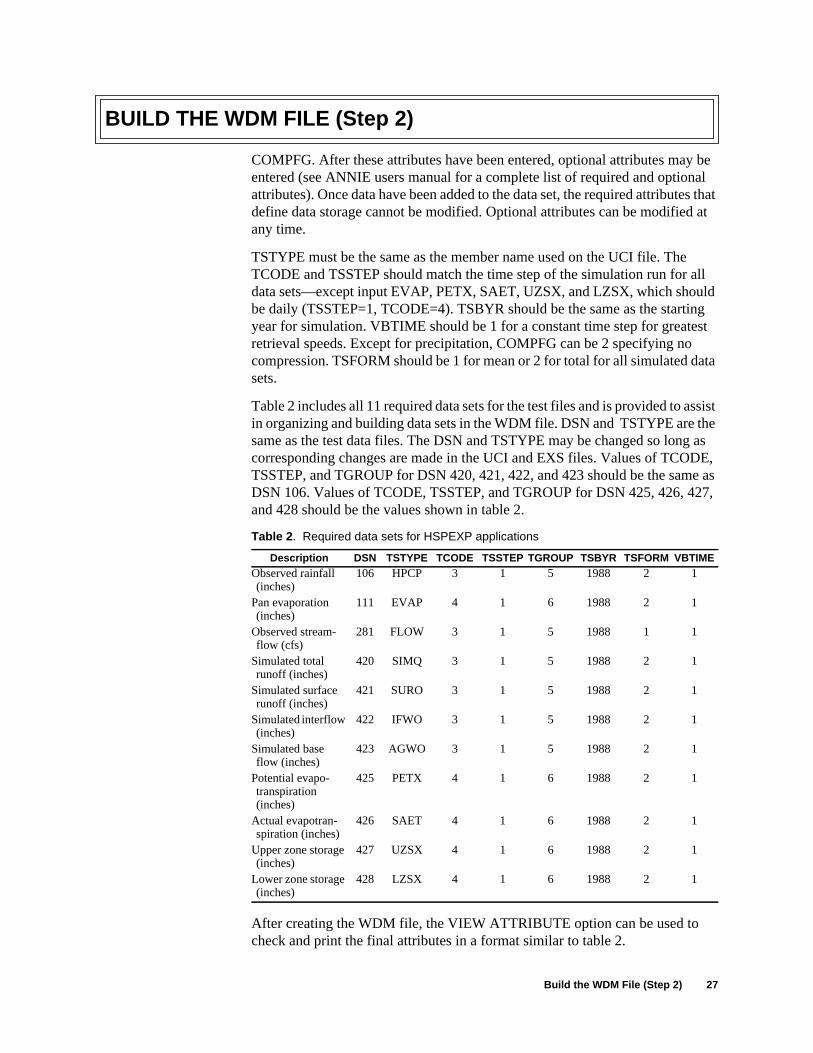
Table 2 includes all 11 required data sets for the test files and is provided to assistin organizing and building data sets in the WDM file. DSN and TSTYPE are thesame as the test data files. The DSN and TSTYPE may be changed so long ascorresponding changes are made in the UCI and EXS files. Values of TCODE,TSSTEP, and TGROUP for DSN 420, 421, 422, and 423 should be the same asDSN 106. Values of TCODE, TSSTEP, and TGROUP for DSN 425, 426, 427,and 428 should be the values shown in table 2.
After creating the WDM file, the VIEW ATTRIBUTE option can be used tocheck and print the final attributes in a format similar to table 2.
Table 2 . Required data sets for HSPEXP applications
Description DSN TSTYPE TCODE TSSTEP TGROUP TSBYR TSFORM VBTIMEObserved rainfall(inches)
106 HPCP 3 1 5 1988 2 1
Pan evaporation(inches)
111 EVAP 4 1 6 1988 2 1
Observed stream-flow (cfs)
281 FLOW 3 1 5 1988 1 1
Simulated totalrunoff (inches)
420 SIMQ 3 1 5 1988 2 1
Simulated surfacerunoff (inches)
421 SURO 3 1 5 1988 2 1
Simulated interflow(inches)
422 IFWO 3 1 5 1988 2 1
Simulated baseflow (inches)
423 AGWO 3 1 5 1988 2 1
Potential evapo-transpiration(inches)
425 PETX 4 1 6 1988 2 1
Actual evapotran-spiration (inches)
426 SAET 4 1 6 1988 2 1
Upper zone storage(inches)
427 UZSX 4 1 6 1988 2 1
Lower zone storage(inches)
428 LZSX 4 1 6 1988 2 1

28 Users Manual for an Expert System (HSPEXP) for Calibration of the Hydrological Simulation Program—Fortran
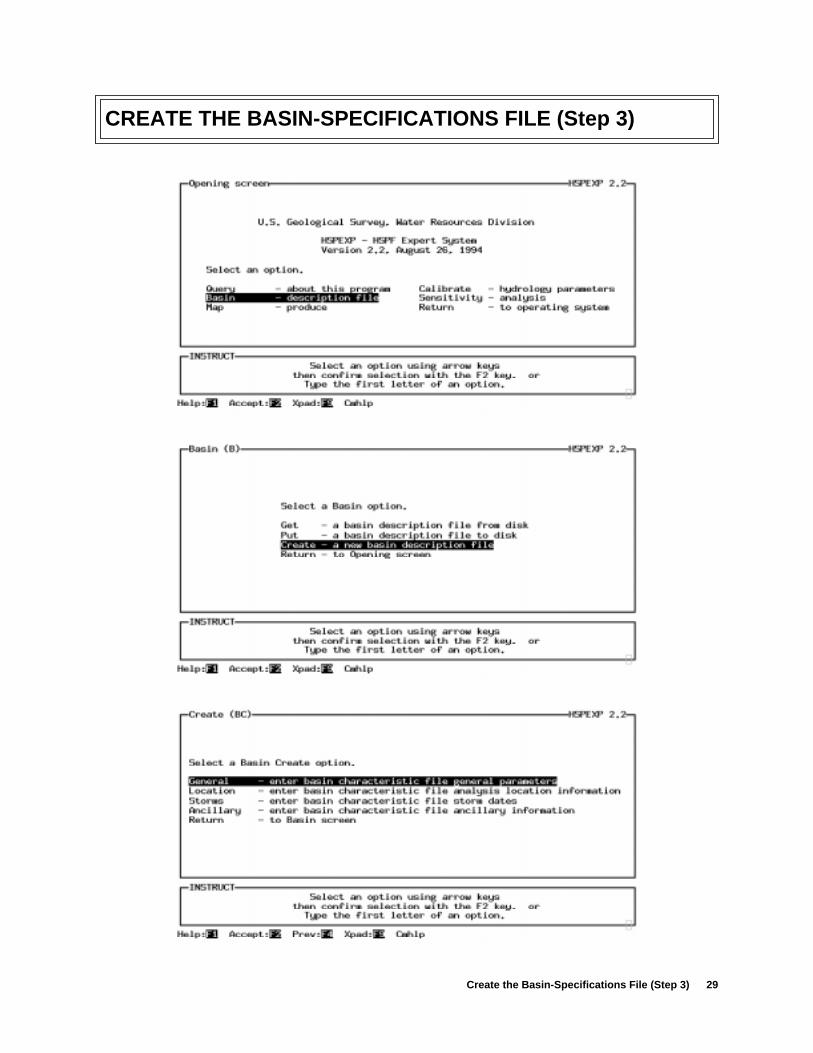
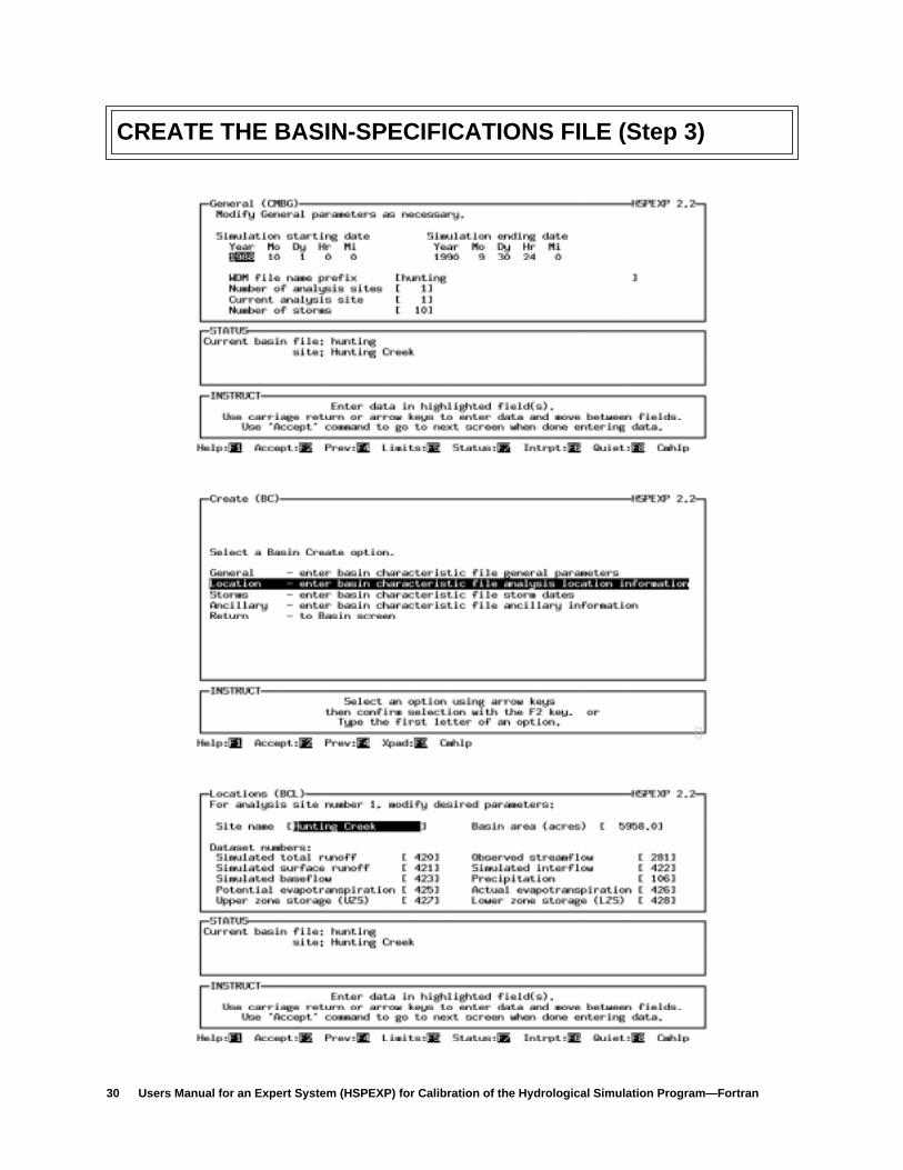
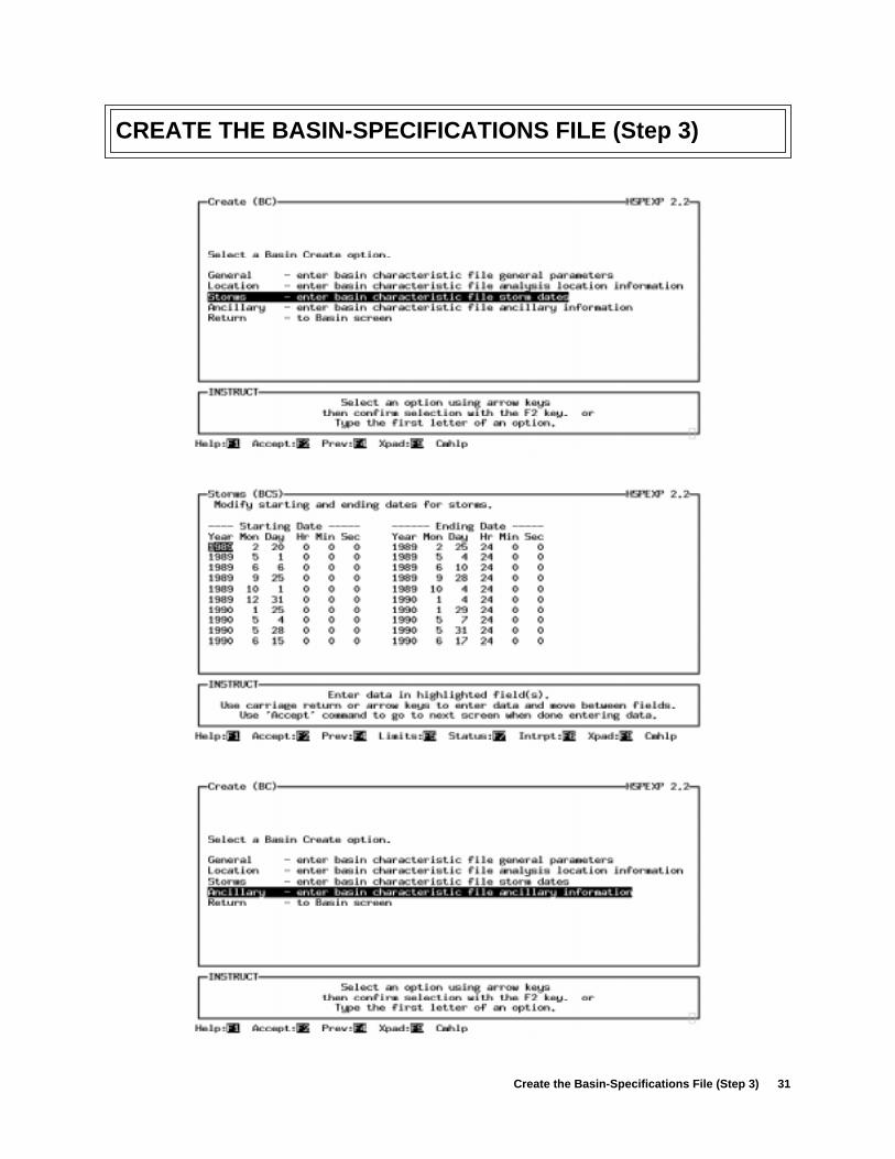
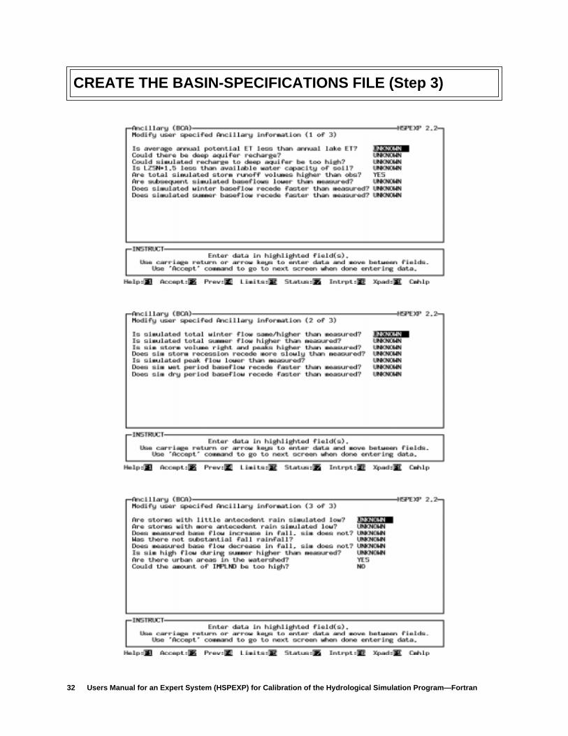
CREATE THE BASIN-SPECIFICATIONS FILE (Step 3)
The CREATE option under the BASIN option in HSPEXP is used to develop theEXS file. There are four options—GENERAL, STORM DATES, LOCATION,and ANCILLARY. The options GENERAL, STORM DATES, and LOCATIONmust be processed; the option ANCILLARY is optional and if not selected,defaults will be used. Items under the GENERAL option must be added. Stormdates must have been previously determined for entry under the STORM DATESoption. To aid in storm date selection, ANNIE can be used to list or plot theprecipitation and observed streamflow data sets. The ANNIE LIST option canlist all precipitation or just the precipitation values above a threshold. TheGRAPHICS option in ANNIE can be used to plot the observed streamflow andprecipitation to visually select the storm periods. Up to 36 storm periods can beentered.
The LOCATION option in HSPEXP identifies the data-set numbers selected inthe previous two steps creating the UCI and WDM files. The LOCATION formprovides a field to enter a basin name to be used on tabular and graphical outputand a field for the drainage area in acres. The ANCILLARY is used to provideadditional information about the drainage basin. This information is used in theexpert system when providing advice. Before leaving the BASIN option, the newEXS file can be saved by using the PUT command.
Below are the menus and forms that are provided in HSPEXP showing the valuesthat were entered for the test data. Following the menus and forms is the resultanthunting.exs file that was produced (fig. 7). Although this file can be edited, it isbetter to modify the values using the expert system. A description of the formatfor the EXS file is presented after the EXS file as table 3.
CREATE
Create the Basin-Specifications File (Step 3) 29
CREATE THE BASIN-SPECIFICATIONS FILE (Step 3)
30 Users Manual for an Expert System (HSPEXP) for Calibration of the Hydrological Simulation Program—Fortran
CREATE THE BASIN-SPECIFICATIONS FILE (Step 3)
Create the Basin-Specifications File (Step 3) 31
CREATE THE BASIN-SPECIFICATIONS FILE (Step 3)
32 Users Manual for an Expert System (HSPEXP) for Calibration of the Hydrological Simulation Program—Fortran
CREATE THE BASIN-SPECIFICATIONS FILE (Step 3)
Create the Basin-Specifications File (Step 3) 33
CREATE THE BASIN-SPECIFICATIONS FILE (Step 3)
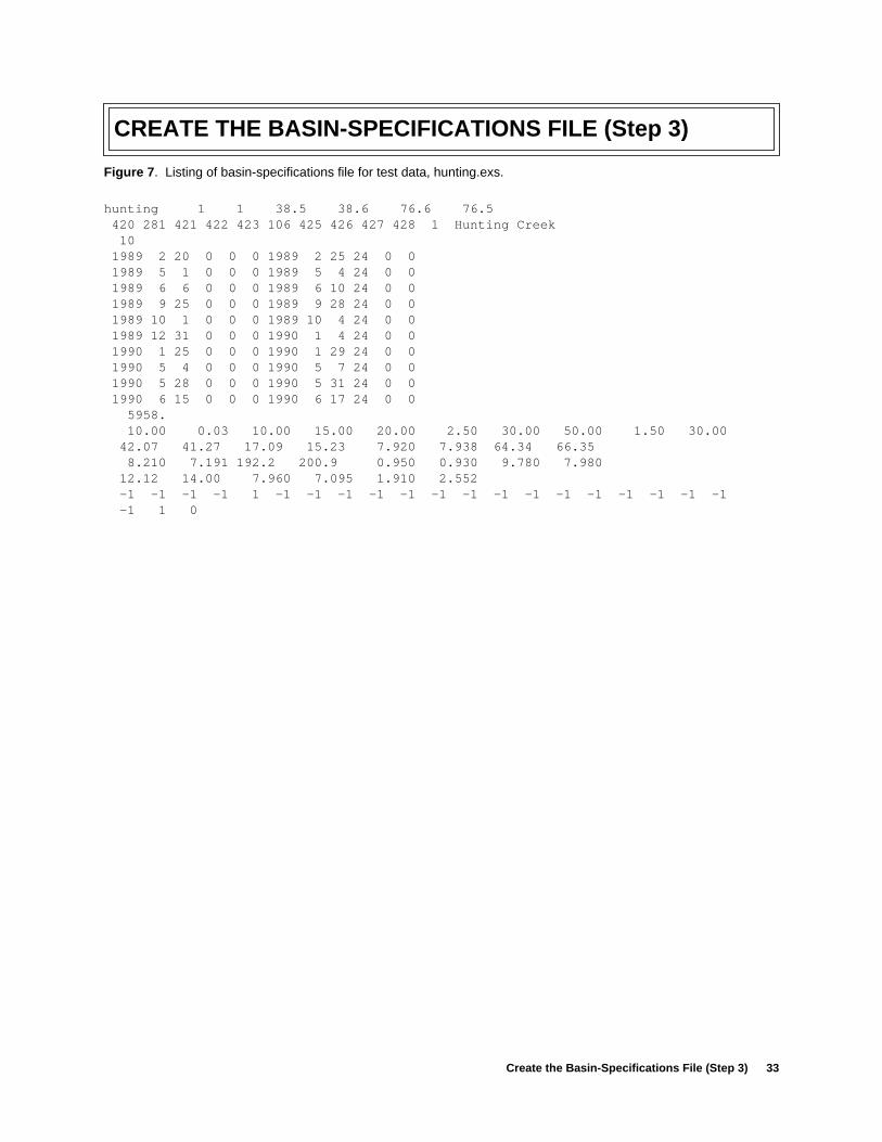
Figure 7 . Listing of basin-specifications file for test data, hunting.exs.
hunting 1 1 38.5 38.6 76.6 76.5 420 281 421 422 423 106 425 426 427 428 1 Hunting Creek 10 1989 2 20 0 0 0 1989 2 25 24 0 0 1989 5 1 0 0 0 1989 5 4 24 0 0 1989 6 6 0 0 0 1989 6 10 24 0 0 1989 9 25 0 0 0 1989 9 28 24 0 0 1989 10 1 0 0 0 1989 10 4 24 0 0 1989 12 31 0 0 0 1990 1 4 24 0 0 1990 1 25 0 0 0 1990 1 29 24 0 0 1990 5 4 0 0 0 1990 5 7 24 0 0 1990 5 28 0 0 0 1990 5 31 24 0 0 1990 6 15 0 0 0 1990 6 17 24 0 0 5958. 10.00 0.03 10.00 15.00 20.00 2.50 30.00 50.00 1.50 30.00 42.07 41.27 17.09 15.23 7.920 7.938 64.34 66.35 8.210 7.191 192.2 200.9 0.950 0.930 9.780 7.980 12.12 14.00 7.960 7.095 1.910 2.552 -1 -1 -1 -1 1 -1 -1 -1 -1 -1 -1 -1 -1 -1 -1 -1 -1 -1 -1 -1 -1 1 0
34 Users Manual for an Expert System (HSPEXP) for Calibration of the Hydrological Simulation Program—Fortran
CREATE THE BASIN-SPECIFICATIONS FILE (Step 3)
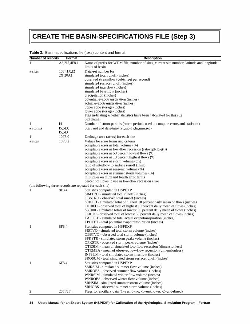
Table 3 . Basin-specifications file (.exs) content and format
Number of records Format Description1 A8,2I5,4F8.1 Name of prefix for WDM file, number of sites, current site number, latitude and longitude
limits of basin# sites 10I4,1X,I2
2X,20A1Data-set number forsimulated total runoff (inches)observed streamflow (cubic feet per second)simulated surface runoff (inches)simulated interflow (inches)simulated base flow (inches)precipitation (inches)potential evapotranspiration (inches)actual evapotranspiration (inches)upper zone storage (inches)lower zone storage (inches)Flag indicating whether statistics have been calculated for this siteSite name
1 I4 Number of storm periods (storm periods used to compute errors and statistics)# storms I5,5I3,
I5,5I3Start and end date/time (yr,mo,dy,hr,min,sec)
1 10F8.0 Drainage area (acres) for each site# sites 10F8.2 Values for error terms and criteria
acceptable error in total volume (%)acceptable error in low-flow recession (ratio q(t-1)/q(t))acceptable error in 50 percent lowest flows (%)acceptable error in 10 percent highest flows (%)acceptable error in storm volumes (%)ratio of interflow to surface runoff (in/in)acceptable error in seasonal volume (%)acceptable error in summer storm volumes (%)multiplier on third and fourth error termspercent of flows to use in low-flow recession error
(the following three records are repeated for each site)1 8F8.4 Statistics computed in HSPEXP
SIMTRO - simulated total runoff (inches)OBSTRO - observed total runoff (inches)S010FD - simulated total of highest 10 percent daily mean of flows (inches)O010FD - observed total of highest 10 percent daily mean of flows (inches)S50100 - simulated totals of lowest 50 percent daily mean of flows (inches)O50100 - observed total of lowest 50 percent daily mean of flows (inches)TACTET - simulated total actual evapotranspiration (inches)TPOTET - total potential evapotranspiration (inches)
1 8F8.4 Statistics computed in HSPEXPSISTVO - simulated total storm volume (inches)OBSTVO - observed total storm volume (inches)SPKSTR - simulated storm peaks volume (inches)OPKSTR - observed storm peaks volume (inches)QTRSIM - mean of simulated low-flow recession (dimensionless)QTRMEA - mean of observed low-flow recession (dimensionless)INFSUM - total simulated storm interflow (inches)SROSUM - total simulated storm surface runoff (inches)
1 6F8.4 Statistics computed in HSPEXPSMRSIM - simulated summer flow volume (inches)SMROBS - observed summer flow volume (inches)WNRSIM - simulated winter flow volume (inches)WNROBS - observed winter flow volume (inches)SRHSIM - simulated summer storm volume (inches)SRHOBS - observed summer storm volume (inches)
2 20I4/3I4 Flags for ancillary data (1=yes, 0=no, -1=unknown, -2=undefined)
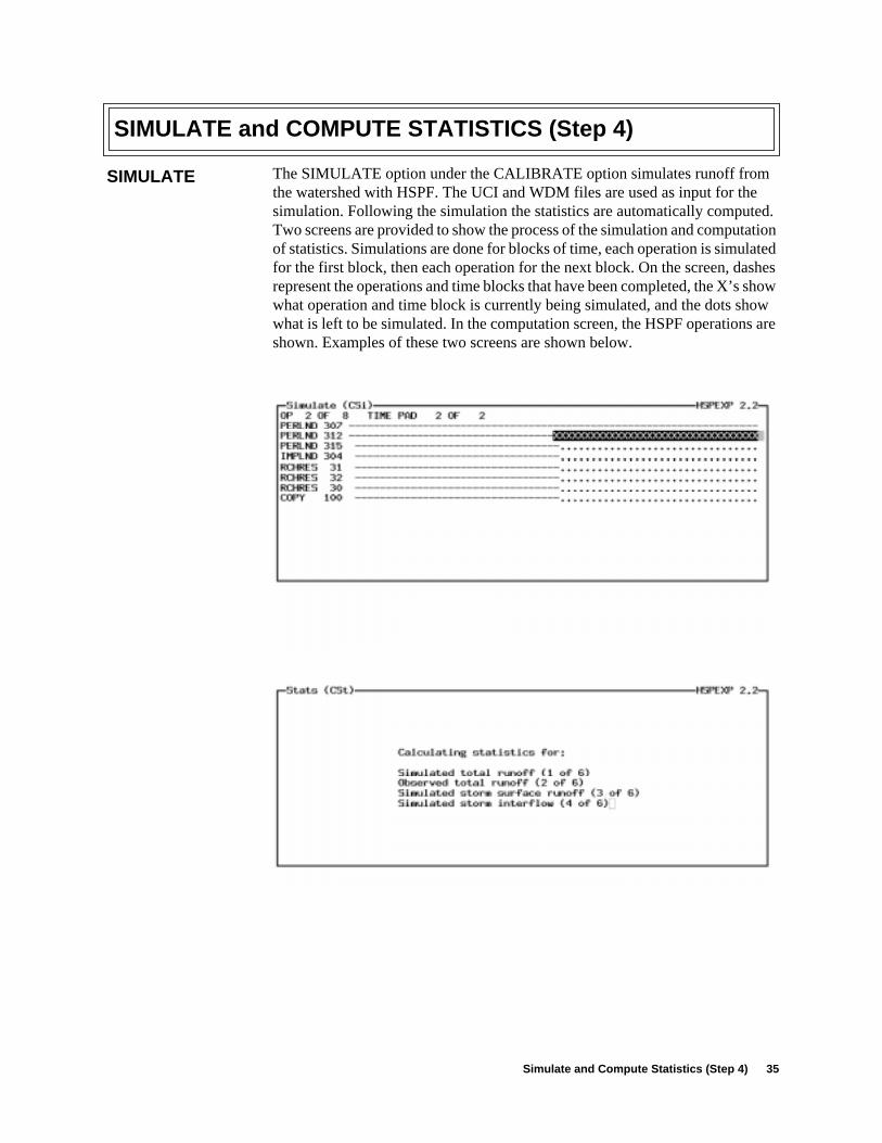
Simulate and Compute Statistics (Step 4) 35
SIMULATE and COMPUTE STATISTICS (Step 4)
The SIMULATE option under the CALIBRATE option simulates runoff fromthe watershed with HSPF. The UCI and WDM files are used as input for thesimulation. Following the simulation the statistics are automatically computed.Two screens are provided to show the process of the simulation and computationof statistics. Simulations are done for blocks of time, each operation is simulatedfor the first block, then each operation for the next block. On the screen, dashesrepresent the operations and time blocks that have been completed, the X’s showwhat operation and time block is currently being simulated, and the dots showwhat is left to be simulated. In the computation screen, the HSPF operations areshown. Examples of these two screens are shown below.
SIMULATE

36 Users Manual for an Expert System (HSPEXP) for Calibration of the Hydrological Simulation Program—Fortran
VIEW GRAPHICS (Step 5)
The first time the graphics option is chosen, the WINDOW option should beselected if you are using a UNIX workstation under X-Windows. This option letsyou select the location of up to four graphs on the screen. The locations are spec-ified by setting the top, bottom, right side, and left side for each graph as a frac-tion of the size of the monitor. You must leave space on the monitor for thewindow to use for the user interface. One graphics X-Window will always beactive and is also specified on the form.
WARNING: When the graphics are displayed under X-Windows, you should notmove, close, or resize the windows using X-Windows because the GraphicalKernel System implementation does not get the information on your changes.Also, if you reset the size and location of the graphic windows and there are cur-rently graphic windows shown, the new sizes will not be used until the next useof HSPEXP.
Use the EDIT TIME option to change the time period and time step for the graph-ics. This is usually used to obtain more detailed results during a shorter period.The time step for storm hydrographs can also be changed on this screen.
When multiple sites of observed streamflow are used for calibration, the EDITSITE option is used to change the site for graphics.
The EDIT Y-AXIS option can be used to select an arithmetic or logarithmic axisfor the daily and storm hydrographs. For the arithmetic axis for daily hydro-graphs, the lower portion of the hydrograph can be plotted to better view the low-flow simulations. A value of 10 percent will enlarge the lowest 10 percent of thehydrograph. The default is 100 percent to show the full hydrographs. The loga-rithmic axis is useful to view low flows and compare recession rates.
The EDIT DEVICE option can be used to send the results to a printer (or post-script file), a metafile (Computer Graphics Metafile), or a pen plotter (or HewlettPackard Graphics Language (HPGL) file).
Select the EDIT PRECIPITATION option to produce plots with precipitation ona separate axis above the monthly, daily, or storm hydrographs.
Select the EDIT COMPONENTS option to also display simulated base flow, andbase flow plus interflow in addition to total simulated runoff. The base-flow andinterflow components have not been routed through the channel reaches, butthese plots usually do not provide a visualization problem unless a reservoir issimulated. When these components are added to the plots, the shading or colorfill options are usually selected under the APPEARANCE option.
Select the EDIT APPEARANCE option to change line type, line color, fill color,or fill pattern for each time series. Fill colors are helpful for simulated flow andrunoff components, but should not be used for observed flow, because that isplotted last and could cover the simulated values. Observed flow is usuallyplotted as a solid line. It is helpful for the precipitation to be plotted as a solid fill.Potential and actual evapotranspiration plots can also use fill colors becausepotential is usually larger and is plotted first.
WINDOW
EDITTIME
EDITSITE
EDITY-AXIS
EDITDEVICE
EDITPRECIPITATION
EDITCOMPONENTS
EDITAPPEARANCE
View Graphics (Step 5) 37
VIEW GRAPHICS (Step 5)
For the bias plots, the type and color of the symbol can be selected.
The DAILY option plots hydrographs of simulated and observed flow (precipita-tion, base flow, and interflow are optional) on a daily time step.
The MONTHLY option plots hydrographs of simulated and observed flow (pre-cipitation, base flow, and interflow are optional) on a monthly time step.
The BIAS option is used to view simulation errors. Three options plot the timeseries of error (simulated-observed) and (1) daily values for the upper zonestorage (UZS), (2) daily values for the lower zone storage (LZS), and (3)observed daily flows. With these plots it can be determined if positive errors ornegative errors result during wet or dry conditions or low flows or high flows. Afourth option plots the average monthly error for each month of the year for allyears to determine if the error has a seasonal pattern.
The WEEKLY ET option plots the actual evapotranspiration (total from allstorage components) and the potential evapotranspiration on a 7-day (weekly)time step. The 7-day time step is used because the impact of evapotranspirationon watershed response is cumulative over periods of several days. The plot helpsassess periods where values of the potential evapotranspiration have most impacton the water balance.
The FLOW-DURATION plot is very useful to view the errors in simulation ofhigh flows relative to simulation of low flows. It is also helpful when the storm-by-storm simulations are poor because of poor rainfall representation. Althoughthe storm-to-storm comparison may be poor, the model may represent theresponse of the watershed properly as shown by a flow-duration curve.
The STORM option lets you plot the simulated and observed flow (precipitation,base flow, and interflow are optional) for each storm period identified on the EXSfile. A menu is provided with a letter for each storm period to select the storm forthe plot. These plots are very useful for adjusting the FTABLE’s for flow routingand fine tuning the parameters for interflow.
The BASE-FLOW RECESSION is a plot of the frequency of simulated andobserved daily recession (Qn/Qn-1) for each day. This plot is used to refine theerror parameter (E10) that defines the percent of time streamflow is in a base-flow condition.
The CUMULATIVE ERROR plot provides information on trends in the simula-tion errors (simulated flow minus observed flows). Overall water-budget prob-lems, seasonal problems, or problems in specific years can be identified on thisplot.
The menus for graphics are shown below. Following those are samples of theplots that were produced (figs. 8-20). On the computer screen, color fill patternswere used. These were changed to dashed and dotted line types for the plots pre-sented. Figure 21 lists the test PLT file and table 4 lists the description of theformat for the PLT file.
EDITMARKER
DAILYPLOT
MONTHLYPLOT
BIASPLOT
WEEKLY ETPLOT
FLOW-DURATIONPLOT
STORMPLOT
BASE-FLOWRECESSIONPLOT
CUMULATIVEERROR PLOT
EXAMPLES
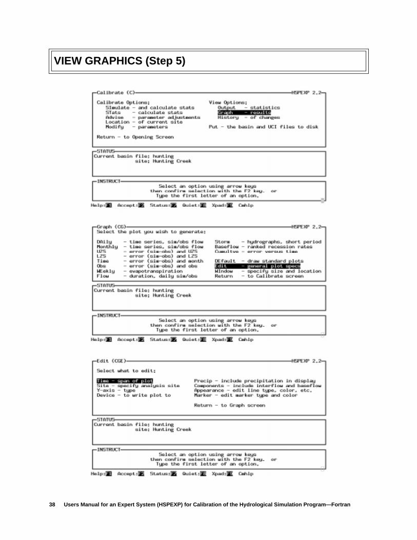
38 Users Manual for an Expert System (HSPEXP) for Calibration of the Hydrological Simulation Program—Fortran
VIEW GRAPHICS (Step 5)
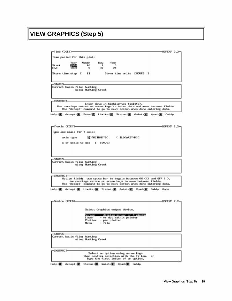
View Graphics (Step 5) 39
VIEW GRAPHICS (Step 5)
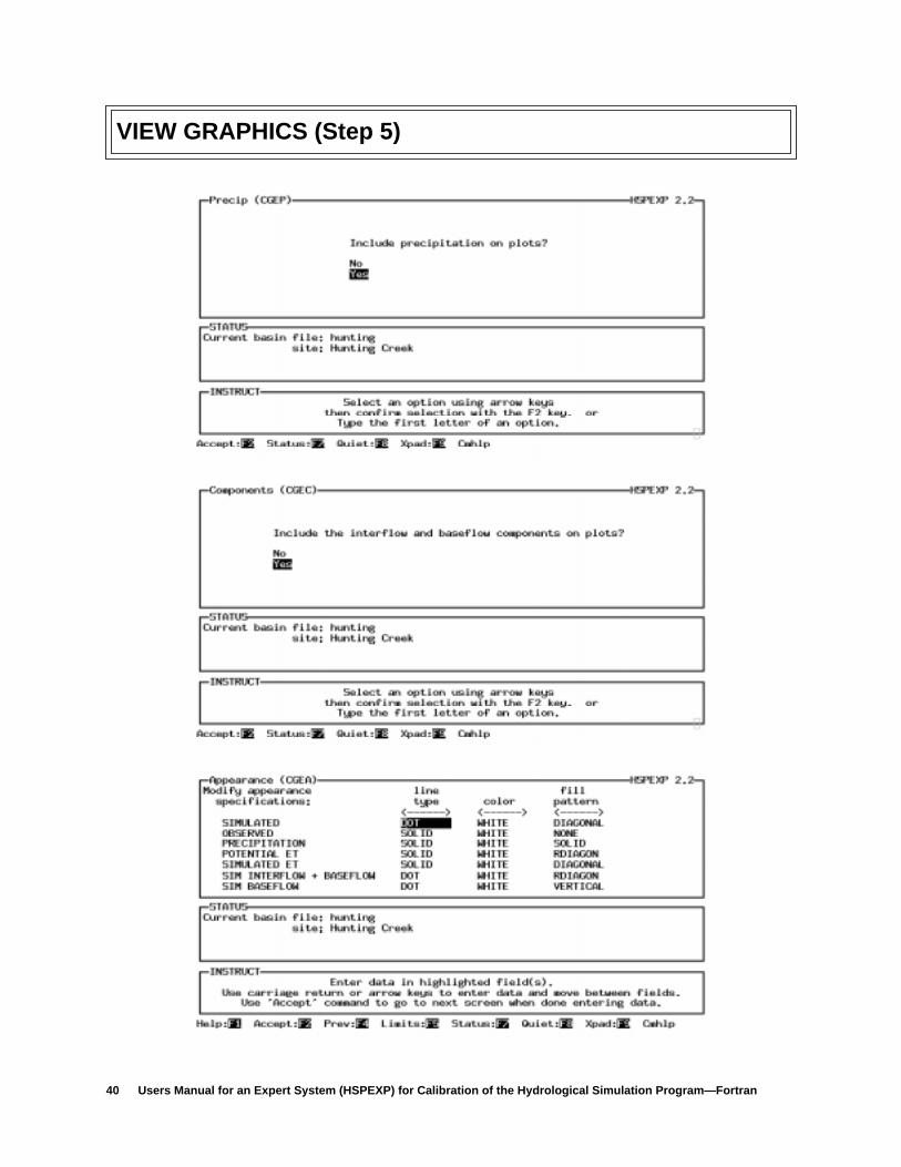
40 Users Manual for an Expert System (HSPEXP) for Calibration of the Hydrological Simulation Program—Fortran
VIEW GRAPHICS (Step 5)
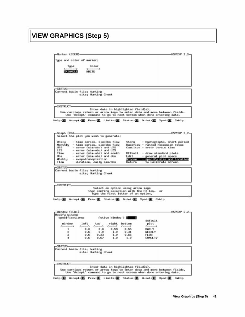
View Graphics (Step 5) 41
VIEW GRAPHICS (Step 5)
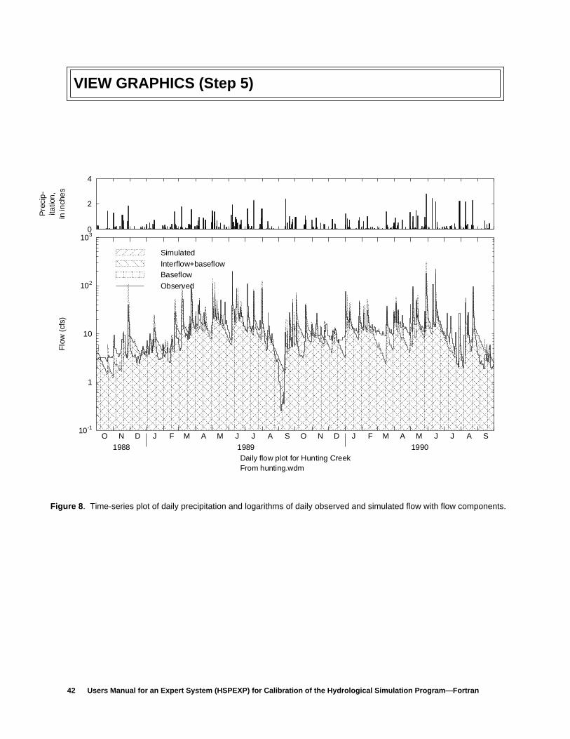
42 Users Manual for an Expert System (HSPEXP) for Calibration of the Hydrological Simulation Program—Fortran
VIEW GRAPHICS (Step 5)
Figure 8 . Time-series plot of daily precipitation and logarithms of daily observed and simulated flow with flow components.
Simulated
Interflow+baseflowBaseflow
Observed
0
2
4
Pre
cip
-ita
tion
,in
inch
es
10-1
1
10
102
103
Flo
w (
cfs)
O N D
1988
J F M A M J J A S O N D
1989
J F M A M J J A S
1990Daily flow plot for Hunting CreekFrom hunting.wdm
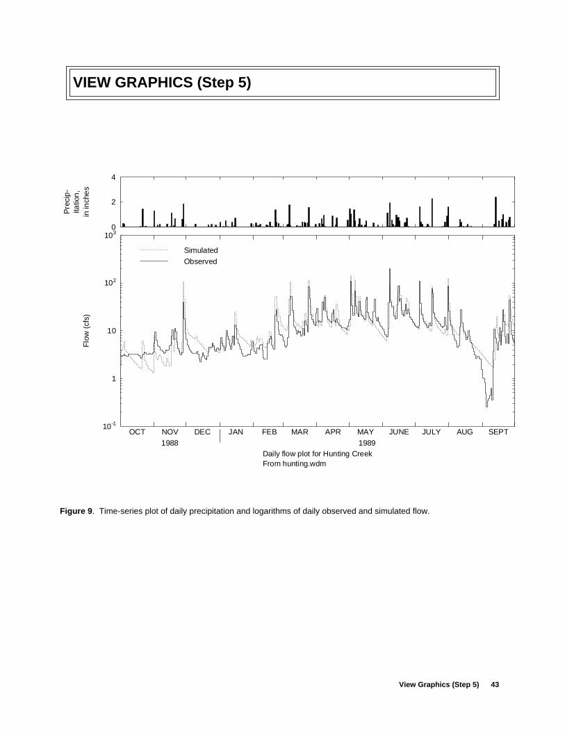
View Graphics (Step 5) 43
VIEW GRAPHICS (Step 5)
Figure 9 . Time-series plot of daily precipitation and logarithms of daily observed and simulated flow.
Simulated
Observed
0
2
4
Pre
cip
-ita
tion
,in
inch
es
10-1
1
10
102
103
Flo
w (
cfs)
OCT NOV DEC
1988
JAN FEB MAR APR MAY JUNE JULY AUG SEPT
1989Daily flow plot for Hunting CreekFrom hunting.wdm
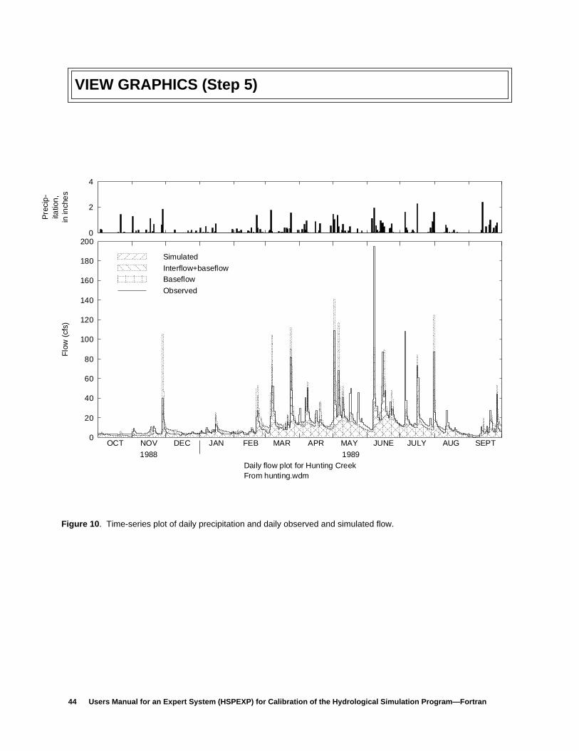
44 Users Manual for an Expert System (HSPEXP) for Calibration of the Hydrological Simulation Program—Fortran
VIEW GRAPHICS (Step 5)
Figure 10 . Time-series plot of daily precipitation and daily observed and simulated flow.
Simulated
Interflow+baseflowBaseflow
Observed
0
2
4
Pre
cip
-ita
tion
,in
inch
es
0
20
40
60
80
100
120
140
160
180
200
Flo
w (
cfs)
OCT NOV DEC
1988
JAN FEB MAR APR MAY JUNE JULY AUG SEPT
1989Daily flow plot for Hunting CreekFrom hunting.wdm
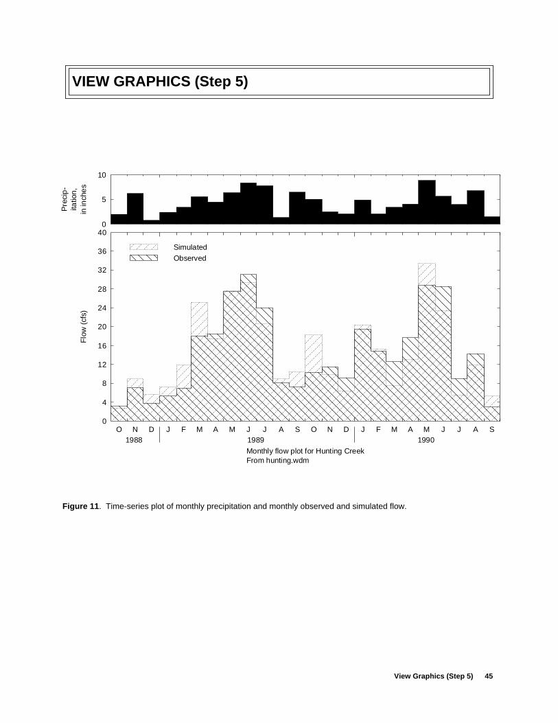
View Graphics (Step 5) 45
VIEW GRAPHICS (Step 5)
Figure 11 . Time-series plot of monthly precipitation and monthly observed and simulated flow.
Simulated
Observed
0
5
10
Pre
cip
-ita
tion
,in
inch
es
0
4
8
12
16
20
24
28
32
36
40
Flo
w (
cfs)
O N D1988
J F M A M J J A S O N D1989
J F M A M J J A S1990
Monthly flow plot for Hunting CreekFrom hunting.wdm

46 Users Manual for an Expert System (HSPEXP) for Calibration of the Hydrological Simulation Program—Fortran
VIEW GRAPHICS (Step 5)
Figure 12 . Plot of the error in daily flows and the simulated daily upper zone storagevalues.
-150
-120
-90
-60
-30
0
30
60
90
120
150
Err
or (
cfs)
0 0.4 0.8 1.2 1.6 2.0 2.4 2.8 3.2 3.6 4.0
UZS (in)Error (sim - obs) vs UZS (daily) for Hunting CreekFrom hunting.wdm
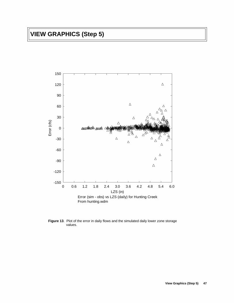
View Graphics (Step 5) 47
VIEW GRAPHICS (Step 5)
Figure 13 . Plot of the error in daily flows and the simulated daily lower zone storagevalues.
-150
-120
-90
-60
-30
0
30
60
90
120
150
Err
or (
cfs)
0 0.6 1.2 1.8 2.4 3.0 3.6 4.2 4.8 5.4 6.0
LZS (in)Error (sim - obs) vs LZS (daily) for Hunting CreekFrom hunting.wdm
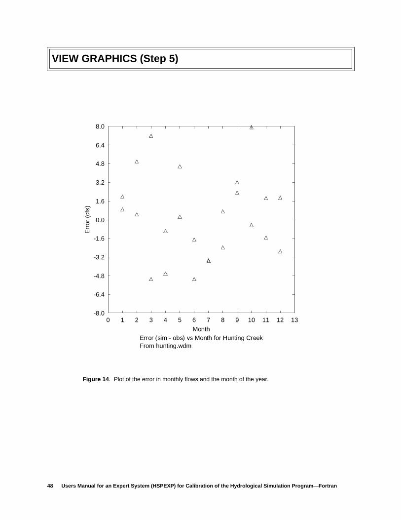
48 Users Manual for an Expert System (HSPEXP) for Calibration of the Hydrological Simulation Program—Fortran
VIEW GRAPHICS (Step 5)
Figure 14 . Plot of the error in monthly flows and the month of the year.
-8.0
-6.4
-4.8
-3.2
-1.6
0.0
1.6
3.2
4.8
6.4
8.0
Err
or (
cfs)
0 1 2 3 4 5 6 7 8 9 10 11 12 13
MonthError (sim - obs) vs Month for Hunting CreekFrom hunting.wdm
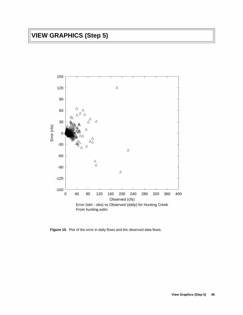
View Graphics (Step 5) 49
VIEW GRAPHICS (Step 5)
Figure 15 . Plot of the error in daily flows and the observed data flows.
-150
-120
-90
-60
-30
0
30
60
90
120
150
Err
or (
cfs)
0 40 80 120 160 200 240 280 320 360 400
Observed (cfs)Error (sim - obs) vs Observed (daily) for Hunting CreekFrom hunting.wdm
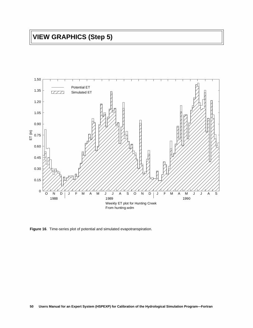
50 Users Manual for an Expert System (HSPEXP) for Calibration of the Hydrological Simulation Program—Fortran
VIEW GRAPHICS (Step 5)
Figure 16 . Time-series plot of potential and simulated evapotranspiration.
Potential ET
Simulated ET
0
0.15
0.30
0.45
0.60
0.75
0.90
1.05
1.20
1.35
1.50
ET
(in
)
O N D
1988
J F M A M J J A S O N D
1989
J F M A M J J A S
1990Weekly ET plot for Hunting CreekFrom hunting.wdm
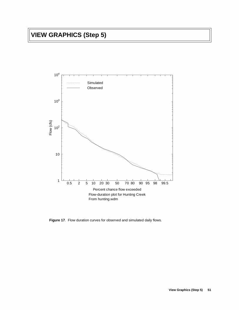
View Graphics (Step 5) 51
VIEW GRAPHICS (Step 5)
Figure 17 . Flow duration curves for observed and simulated daily flows.
SimulatedObserved
1
10
102
103
104
Flo
w (
cfs)
0.5 2 5 10 20 30 50 70 80 90 95 98 99.5
Percent chance flow exceededFlow-duration plot for Hunting CreekFrom hunting.wdm
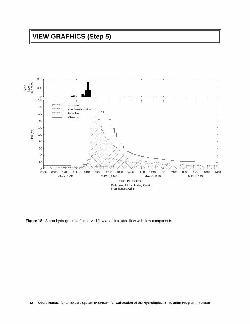
52 Users Manual for an Expert System (HSPEXP) for Calibration of the Hydrological Simulation Program—Fortran
VIEW GRAPHICS (Step 5)
Figure 18 . Storm hydrographs of observed flow and simulated flow with flow components.
Simulated
Interflow+baseflowBaseflow
Observed
0
0.4
0.8
Pre
cip
-ita
tion,
in in
ches
0
20
40
60
80
100
120
140
160
180
200
Flo
w (
cfs)
0000 0600 1200 1800
MAY 4, 1990
2400 0600 1200 1800
MAY 5, 1990
2400 0600 1200 1800
MAY 6, 1990
2400 0600 1200 1800
MAY 7, 1990
2400
TIME, IN HOURS
Daily flow plot for Hunting CreekFrom hunting.wdm
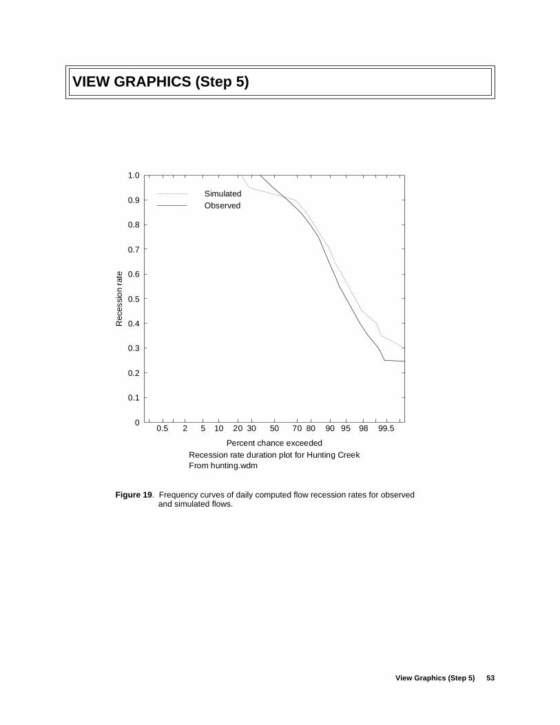
View Graphics (Step 5) 53
VIEW GRAPHICS (Step 5)
Figure 19 . Frequency curves of daily computed flow recession rates for observedand simulated flows.
SimulatedObserved
0
0.1
0.2
0.3
0.4
0.5
0.6
0.7
0.8
0.9
1.0
Rec
essi
on
rate
0.5 2 5 10 20 30 50 70 80 90 95 98 99.5
Percent chance exceededRecession rate duration plot for Hunting CreekFrom hunting.wdm
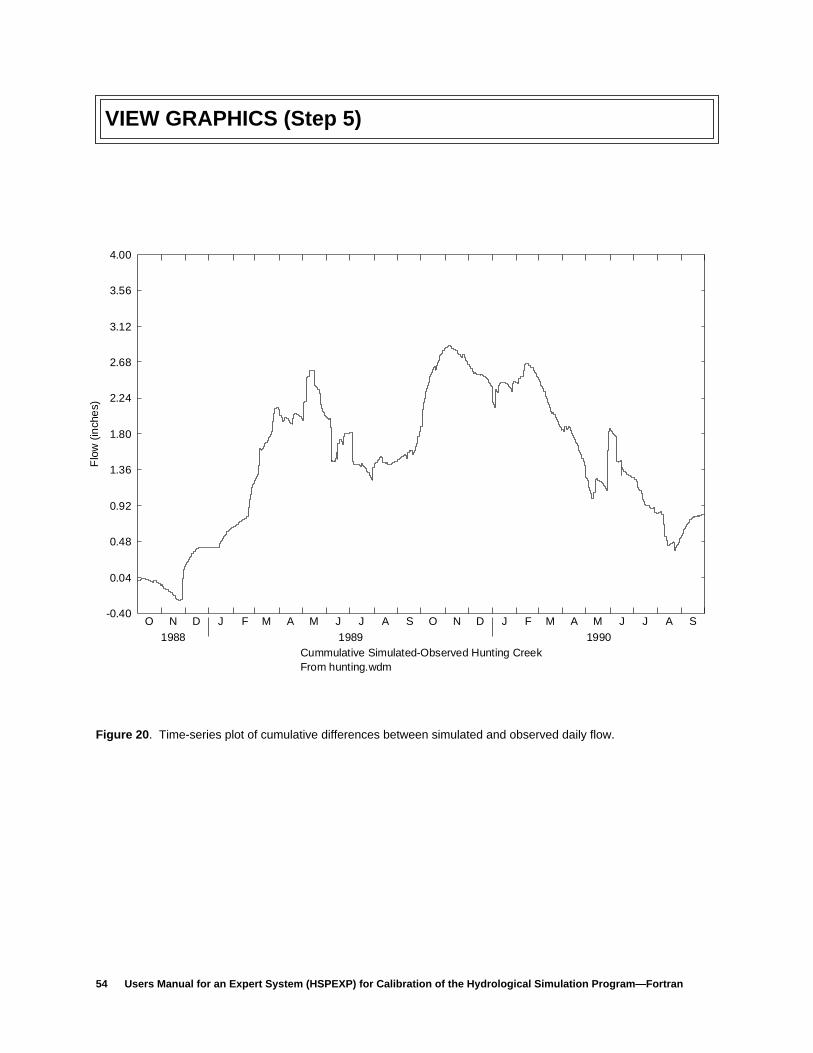
54 Users Manual for an Expert System (HSPEXP) for Calibration of the Hydrological Simulation Program—Fortran
VIEW GRAPHICS (Step 5)
Figure 20 . Time-series plot of cumulative differences between simulated and observed daily flow.
-0.40
0.04
0.48
0.92
1.36
1.80
2.24
2.68
3.12
3.56
4.00
Flo
w (
inch
es)
O N D
1988
J F M A M J J A S O N D
1989
J F M A M J J A S
1990Cummulative Simulated-Observed Hunting CreekFrom hunting.wdm
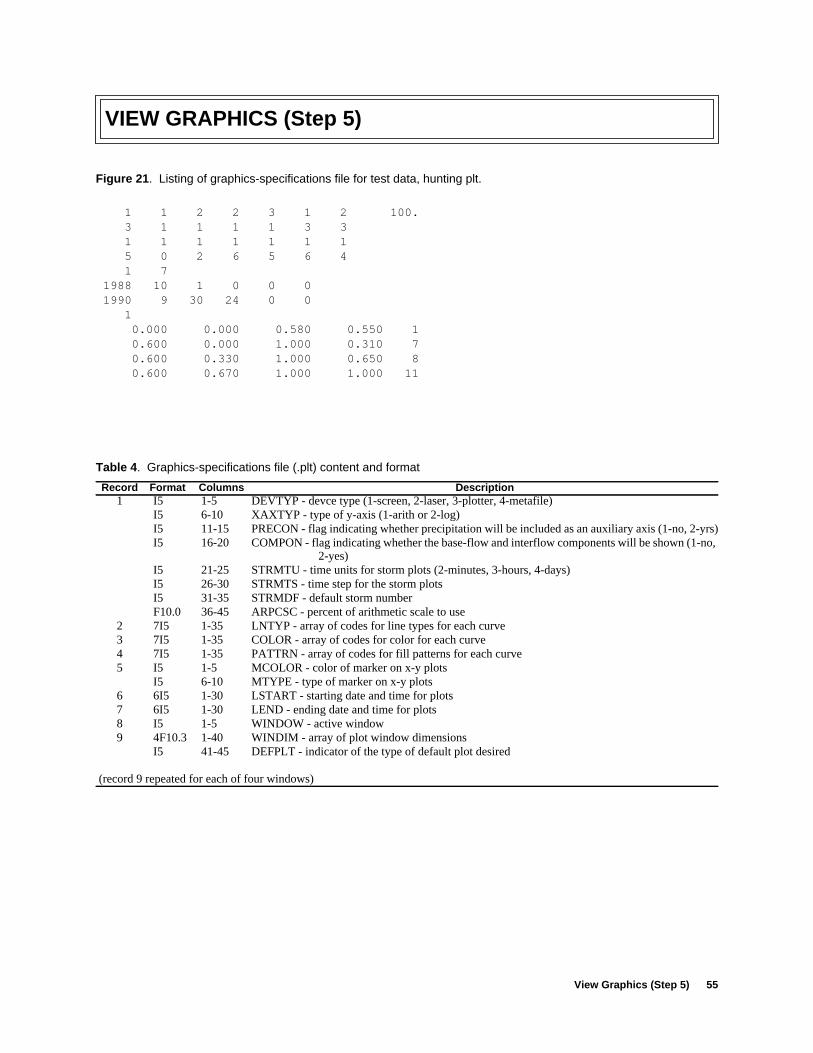
View Graphics (Step 5) 55
VIEW GRAPHICS (Step 5)
Figure 21 . Listing of graphics-specifications file for test data, hunting plt.
1 1 2 2 3 1 2 100. 3 1 1 1 1 3 3 1 1 1 1 1 1 1 5 0 2 6 5 6 4 1 7 1988 10 1 0 0 0 1990 9 30 24 0 0 1 0.000 0.000 0.580 0.550 1 0.600 0.000 1.000 0.310 7 0.600 0.330 1.000 0.650 8 0.600 0.670 1.000 1.000 11
Table 4 . Graphics-specifications file (.plt) content and format
Record Format Columns Description1 I5 1-5 DEVTYP - devce type (1-screen, 2-laser, 3-plotter, 4-metafile)
I5 6-10 XAXTYP - type of y-axis (1-arith or 2-log)I5 11-15 PRECON - flag indicating whether precipitation will be included as an auxiliary axis (1-no, 2-yrs)I5 16-20 COMPON - flag indicating whether the base-flow and interflow components will be shown (1-no,
2-yes)I5 21-25 STRMTU - time units for storm plots (2-minutes, 3-hours, 4-days)I5 26-30 STRMTS - time step for the storm plotsI5 31-35 STRMDF - default storm numberF10.0 36-45 ARPCSC - percent of arithmetic scale to use
2 7I5 1-35 LNTYP - array of codes for line types for each curve3 7I5 1-35 COLOR - array of codes for color for each curve4 7I5 1-35 PATTRN - array of codes for fill patterns for each curve5 I5 1-5 MCOLOR - color of marker on x-y plots
I5 6-10 MTYPE - type of marker on x-y plots6 6I5 1-30 LSTART - starting date and time for plots7 6I5 1-30 LEND - ending date and time for plots8 I5 1-5 WINDOW - active window9 4F10.3 1-40 WINDIM - array of plot window dimensions
I5 41-45 DEFPLT - indicator of the type of default plot desired
(record 9 repeated for each of four windows)
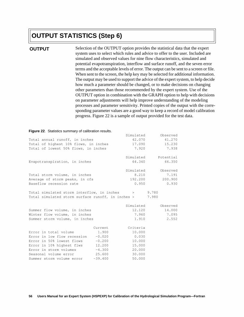
56 Users Manual for an Expert System (HSPEXP) for Calibration of the Hydrological Simulation Program—Fortran
OUTPUT STATISTICS (Step 6)
Selection of the OUTPUT option provides the statistical data that the expertsystem uses to select which rules and advice to offer to the user. Included aresimulated and observed values for nine flow characteristics, simulated andpotential evapotranspiration, interflow and surface runoff, and the seven errorterms and the acceptable levels of error. The output can be sent to a screen or file.When sent to the screen, the help key may be selected for additional information.The output may be used to support the advice of the expert system, to help decidehow much a parameter should be changed, or to make decisions on changingother parameters than those recommended by the expert system. Use of theOUTPUT option in combination with the GRAPH option to help with decisionson parameter adjustments will help improve understanding of the modelingprocesses and parameter sensitivity. Printed copies of the output with the corre-sponding parameter values are a good way to keep a record of model calibrationprogress. Figure 22 is a sample of output provided for the test data.
Figure 22 . Statistics summary of calibration results. Simulated ObservedTotal annual runoff, in inches 42.070 41.270Total of highest 10% flows, in inches 17.090 15.230Total of lowest 50% flows, in inches 7.920 7.938
Simulated PotentialEvapotranspiration, in inches 64.340 66.350
Simulated ObservedTotal storm volume, in inches 8.210 7.191Average of storm peaks, in cfs 192.200 200.900Baseflow recession rate 0.950 0.930
Total simulated storm interflow, in inches > 9.780Total simulated storm surface runoff, in inches > 7.980
Simulated ObservedSummer flow volume, in inches 12.120 14.000Winter flow volume, in inches 7.960 7.095Summer storm volume, in inches 1.910 2.552
Current CriteriaError in total volume 1.900 10.000Error in low flow recession -0.020 0.030Error in 50% lowest flows -0.200 10.000Error in 10% highest flws 12.200 15.000Error in storm volumes -4.300 20.000Seasonal volume error 25.600 30.000Summer storm volume error -39.400 50.000
OUTPUT
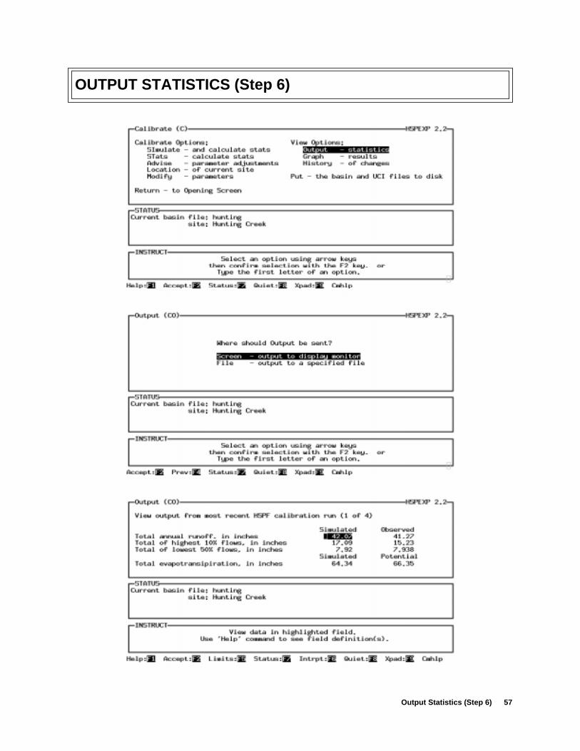
Output Statistics (Step 6) 57
OUTPUT STATISTICS (Step 6)
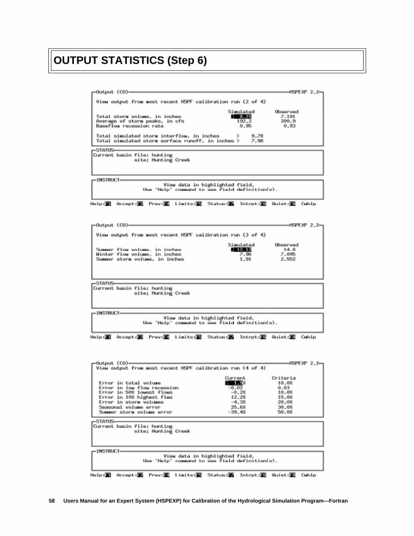
58 Users Manual for an Expert System (HSPEXP) for Calibration of the Hydrological Simulation Program—Fortran
OUTPUT STATISTICS (Step 6)
Check Calibration Advice (Step 7) 59
CHECK CALIBRATION ADVICE (Step 7)
Calibration advice from the expert system is provided by selecting the ADVISEoption. The advice can be sent to a file or to the screen. The advice has threeparts: (1) the conditions that cause the advice to be given, (2) the advice that sug-gests an increase or decrease in a parameter value, and (3) why the advice isgiven for the stated conditions. The amount to change a parameter is not pro-vided. If the change is too small, you will likely get the advice again. If thechange is too large, the next advice may be to change the parameter in the otherdirection.
Usually one screen is provided but in some cases two or three screens maycontain changes. The following is a sample of the advice provided for the testdata. A complete listing of the advice is presented in Appendix A.
ADVISE

60 Users Manual for an Expert System (HSPEXP) for Calibration of the Hydrological Simulation Program—Fortran
CHECK CALIBRATION ADVICE (Step 7)
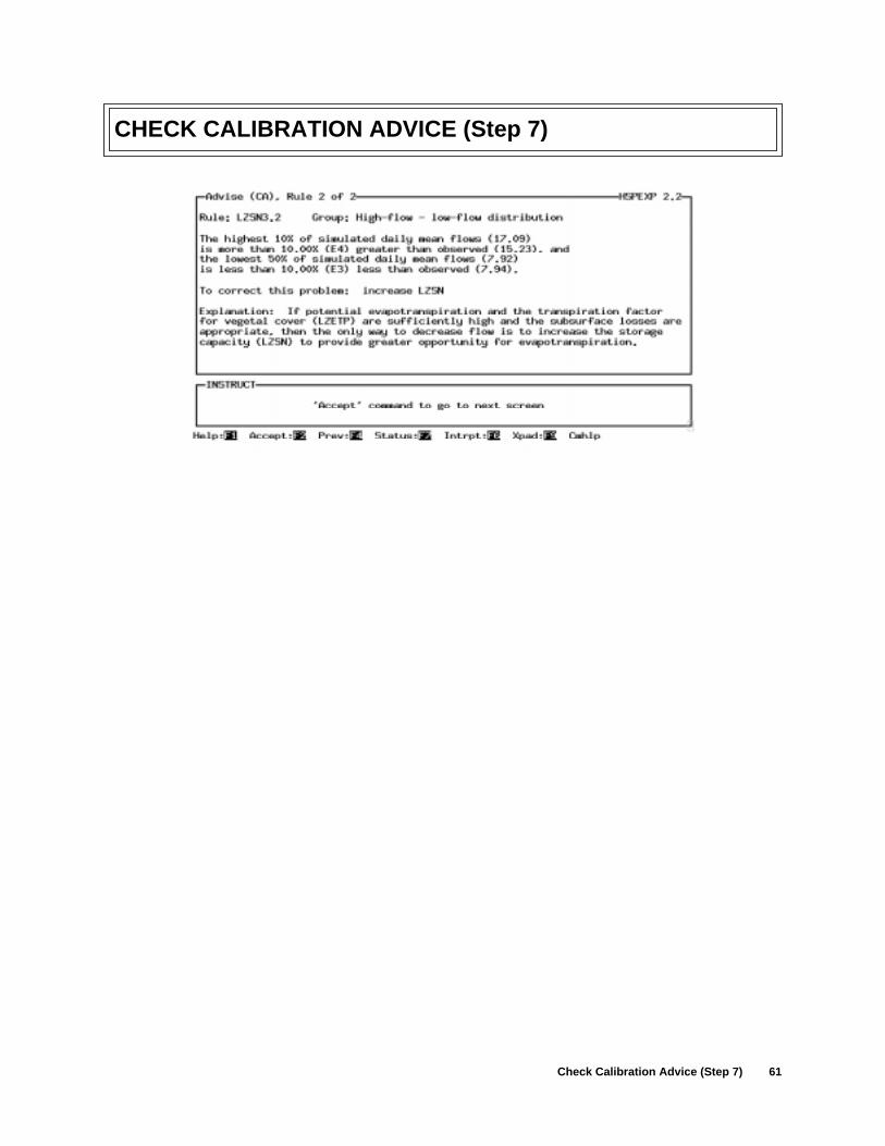
Check Calibration Advice (Step 7) 61
CHECK CALIBRATION ADVICE (Step 7)
62 Users Manual for an Expert System (HSPEXP) for Calibration of the Hydrological Simulation Program—Fortran
ADJUST PARAMETERS (Step 8)
The MODIFY option is selected to adjust parameters in the UCI file. UnderMODIFY there are two options, PARAMETERS and UCI, which may be usedto modify HSPF parameters. PARAMETERS is a simple option for changing thebasic PERLND parameters by parameter name for all PERLND’s or all parame-ters for a specific PERLND. When several PERLND’s are used and the advicehas suggested changing only one parameter, the PARAMETERS option wouldbe most useful.
Anything in the UCI file can be changed with the UCI option. This would beneeded to add a monthly table for a PERLND parameter, modify an FTABLE, orchange the area for an IMPLND or PERLND in the SCHEMATIC block. Themenus for the UCI option are organized in the same way as the UCI file, byblocks and tables. First the block of interest is selected, then one or more specifictables within a block are selected. Each of the selected tables are then displayedfor editing. The parameter description (F1) key and parameter range (F5) key areavailable for each item in each table. There are over 300 tables that can beselected and edited. Only changes to existing operations in the UCI file can bemade. The addition of new operations in the UCI file must be done in a texteditor.
Presented below are the screens that can be used to make the parameter changesuggested in the advice. Both the PARAMETER and UCI options are illustrated.
MODIFY
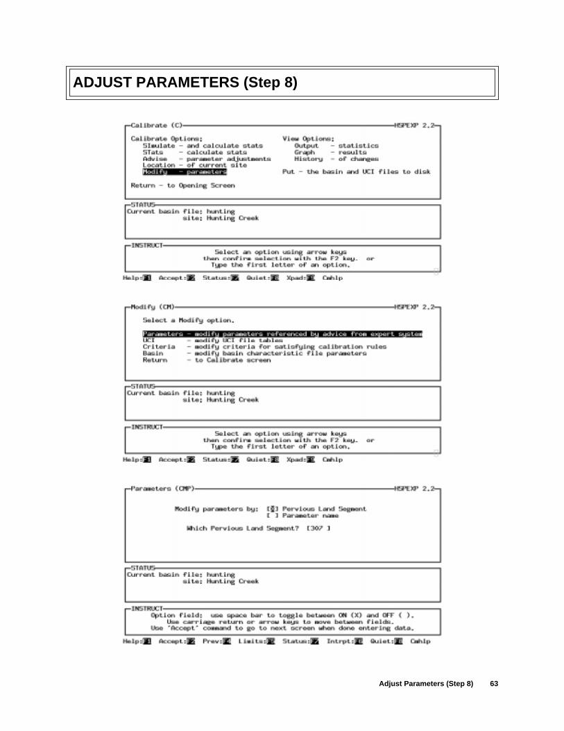
Adjust Parameters (Step 8) 63
ADJUST PARAMETERS (Step 8)
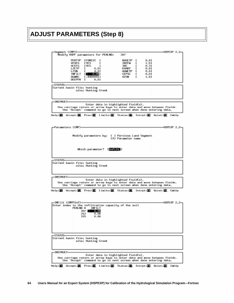
64 Users Manual for an Expert System (HSPEXP) for Calibration of the Hydrological Simulation Program—Fortran
ADJUST PARAMETERS (Step 8)
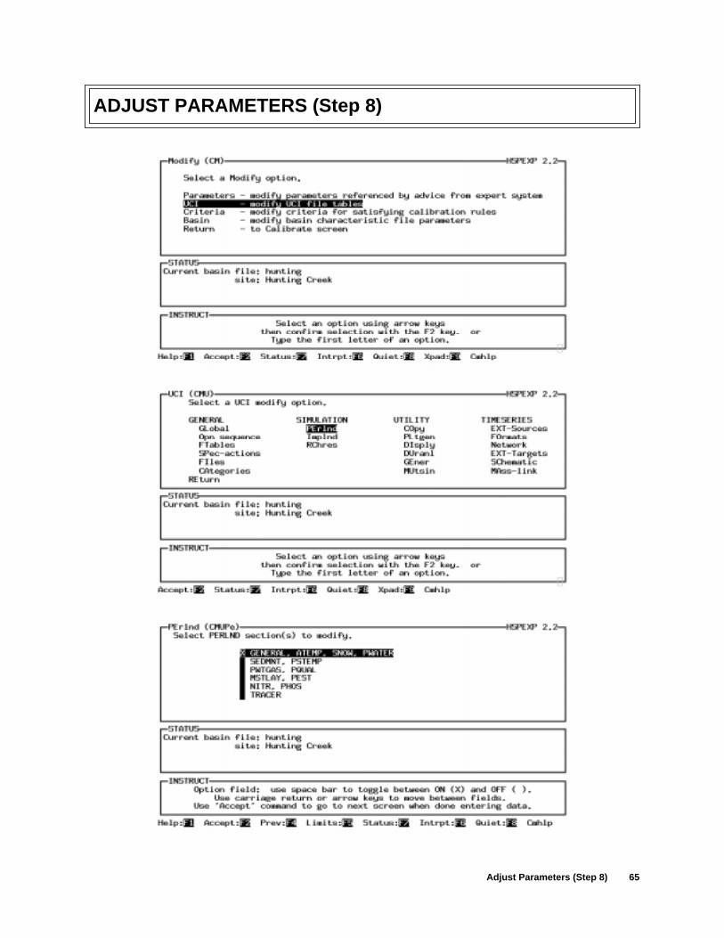
Adjust Parameters (Step 8) 65
ADJUST PARAMETERS (Step 8)
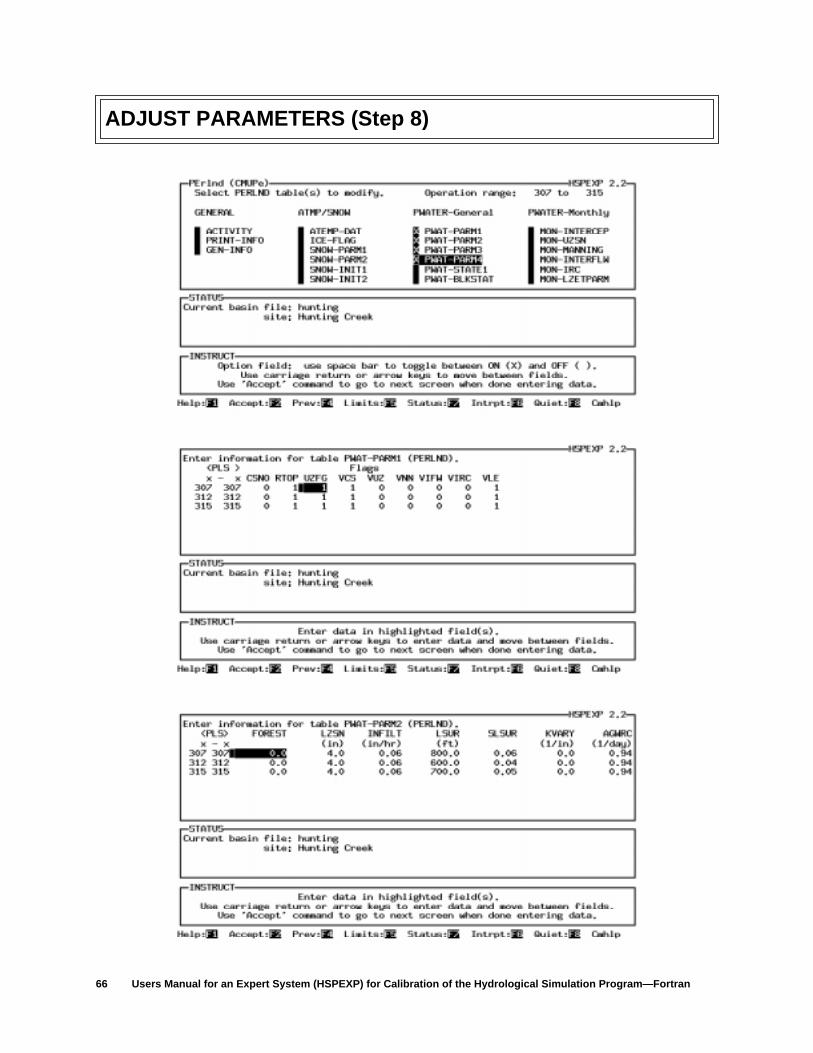
66 Users Manual for an Expert System (HSPEXP) for Calibration of the Hydrological Simulation Program—Fortran
ADJUST PARAMETERS (Step 8)

Modify Error Criteria (Step 9) 67
MODIFY ERROR CRITERIA (Step 9)
To modify the error criteria, select the CRITERIA option of the MODIFY menu.The 10 terms (E1-E10) and their values will be displayed. Seven terms areacceptable levels of error (E1-E5, E7, and E8), two terms (E6 and E9) adjustsome of the values used in the rules, and one term (E10) impacts the computationof the error in base-flow recession. E6 impacts rules for the interflow parametersIRC and INTFW and should not be changed. E9 is used to compute the error termfor the volume rule for the infiltration parameter INFILT and is a multiplier onthe error term that is used in the low-flow rule for INFILT. The value for E10 canbe determined by viewing the base-flow recession plot. From the plot determinethe percent of time the observed recession was between a lower limit and 1.0.The lower limit would usually be between 0.85 and 0.95. The default criteria is30 percent, which would usually be too high for arid and semi-arid regions wherethe stream is dry most of the time.
If no advice is given because the computed error terms are within the acceptablelevels of error, the acceptable levels criteria can be reduced to attempt to refinethe calibration. There is a point where no parameter sets can meet all criteriaresulting in an infinite loop adjusting and readjusting with no real gains. At thispoint, calibration should end.
There may be an error criterion that cannot be met such as the acceptable levelof error for summer storm volumes and the calibration cannot get past that step.This may be caused by large errors in the observed data or storms not well rep-resented by a single rain gage. In this case, the error criteria for summer stormvolumes could be increased so that the additional types of errors can beaddressed.
CRITERIA
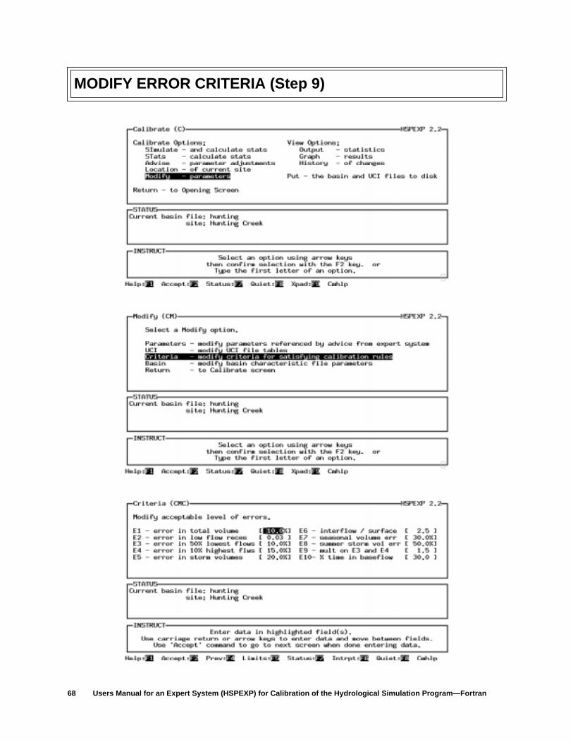
68 Users Manual for an Expert System (HSPEXP) for Calibration of the Hydrological Simulation Program—Fortran
MODIFY ERROR CRITERIA (Step 9)
References 69
SELECTED REFERENCES
Donigian, A.S., Jr., Imhoff, J.C., Bicknell, Brian, Kittle, J.L., Jr., 1984, Application guide for HydrologicalSimulation Program—Fortran (HSPF): U.S. Environmental Protection Agency, Environmental ResearchLaboratory, Athens, Ga., EPA-600/3-84-065, 177 p.
Gaschnig, John, Reboh, Rene, and Reiter, John, 1981, Development of a knowledge-based expert system for waterresources problems: Final Report, SRI Project 1619, SRI International, Menlo Park, Calif., 133 p.
Bicknell, B.R., Imhoff, J.C., Kittle, J.L., Jr., Donigian, A.S., and Johanson, R.C., 1993, Hydrological SimulationProgram—Fortran, Users Manual for Release 10: EPA-600/R-93/174, Environmental Research Laboratory,Athens, Ga., 660 p.
James, L.D., 1972, Hydrologic modeling, parameter estimation, and watershed characteristics: Journal of Hydrology,v. 17, p. 283-307.
Kittle, J.L., Jr., Hummel, P.R., and Imhoff, J.C., 1989, ANNIE-IDE, A system for developing interactive userinterfaces for environmental models (Programmers Guide): EPA/600/3-89/034, Environmental ResearchLaboratory, Athens, Ga., 166 p.
Kohler, M.A., Nordenson, T.J., and Fox, W.E., 1955, Evaporation from pans and lakes: U.S. Department ofCommerce, Weather Bureau, Research Paper No. 38, Washington, D.C., 21 p.
Lumb, A.M., Kittle, J.L., Jr., and Flynn, K.M., 1990, Users manual for ANNIE, A computer program for interactivehydrologic analysis and data management: U.S. Geological Survey Water-Resources Investigations Report89-4080, 236 p.
Lumb, A.M., and McCammon, R.B., 1991, HYDRO-II, An expert system for watershed model calibration:Proceedings of the Seventh International Conference on Interactive Information and Processing Systems forMeteorology, Oceanography and Hydrology, American Meteorological Society, New Orleans, La., January 14-18, 1991, p. 324-327.
Stefik, Mark, Bobrow, D.G., Mittal, Sanjay, and Conway, Lynn, 1983, Knowledge programming in LOOPS—Reporton an experimental course: AI Magazine, v. 4, no. 3, p. 3-13.

70 Users Manual for an Expert System (HSPEXP) for Calibration of the Hydrological Simulation Program—Fortran

__________________________________________
APPENDIXES
__________________________________________

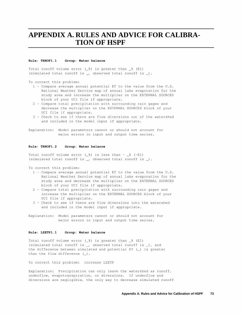
Appendix A. Rules and Advice for Calibration of HSPF 73
APPENDIX A. RULES AND ADVICE FOR CALIBRA-TION OF HSPF
Rule: TRNOF1.1 Group: Water balance
Total runoff volume error (_%) is greater than _% (E1)(simulated total runoff is _, observed total runoff is _).
To correct this problem: 1 - Compare average annual potential ET to the value from the U.S. National Weather Service map of annual lake evaporation for the study area and increase the multiplier on the EXTERNAL SOURCES block of your UCI file if appropriate. 2 - Compare total precipitation with surrounding rain gages and decrease the multiplier on the EXTERNAL SOURCES block of your UCI file if appropriate. 3 - Check to see if there are flow diversions out of the watershed and included in the model input if appropriate.
Explanation: Model parameters cannot or should not account for major errors in input and output time series.
Rule: TRNOF1.2 Group: Water balance
Total runoff volume error (_%) is less than - _% (-E1)(simulated total runoff is _, observed total runoff is _).
To correct this problem: 1 - Compare average annual potential ET to the value from the U.S. National Weather Service map of annual lake evaporation for the study area and decrease the multiplier on the EXTERNAL SOURCES block of your UCI file if appropriate. 2 - Compare total precipitation with surrounding rain gages and increase the multiplier on the EXTERNAL SOURCES block of your UCI file if appropriate. 3 - Check to see if there are flow diversions into the watershed and included in the model input if appropriate.
Explanation: Model parameters cannot or should not account for major errors in input and output time series.
Rule: LZETP1.1 Group: Water balance
Total runoff volume error (_%) is greater than _% (E1)(simulated total runoff is _, observed total runoff is _), andthe difference between simulated and potential ET (_) is greaterthan the flow difference (_).
To correct this problem: increase LZETP
Explanation: Precipitation can only leave the watershed as runoff,underflow, evapotranspiration, or diversions. If underflow anddiversions are negligible, the only way to decrease simulated runoff
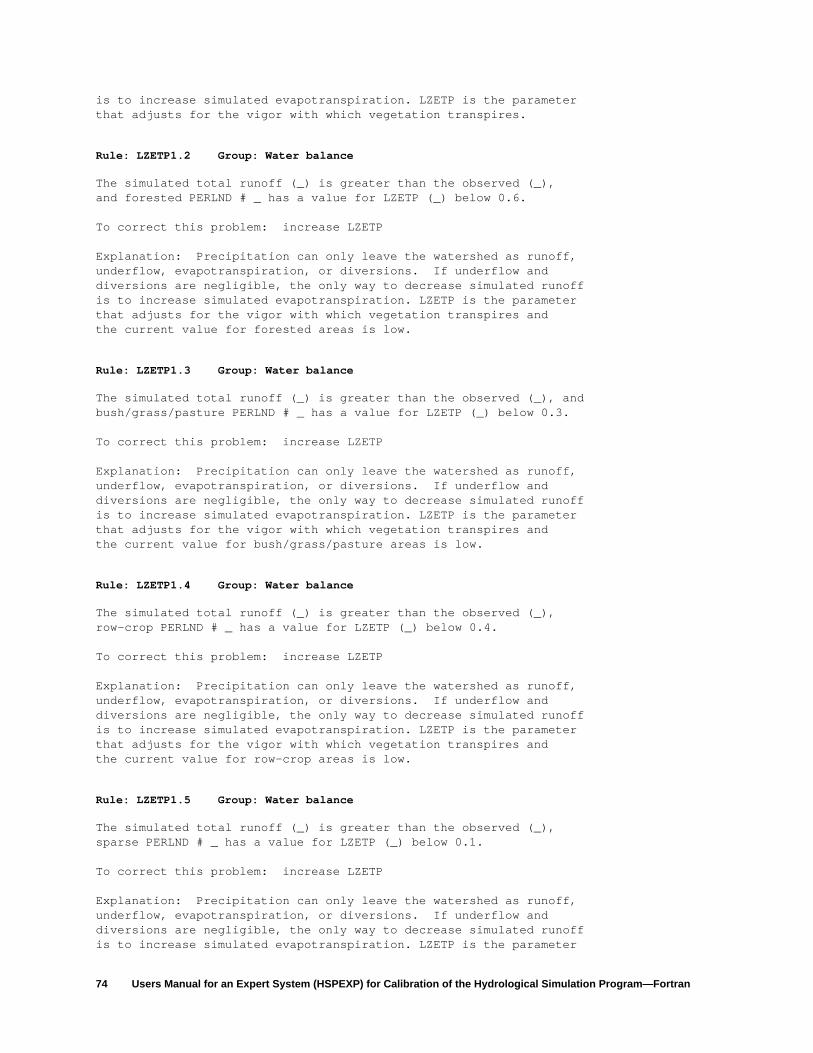
74 Users Manual for an Expert System (HSPEXP) for Calibration of the Hydrological Simulation Program—Fortran
is to increase simulated evapotranspiration. LZETP is the parameterthat adjusts for the vigor with which vegetation transpires.
Rule: LZETP1.2 Group: Water balance
The simulated total runoff (_) is greater than the observed (_),and forested PERLND # _ has a value for LZETP (_) below 0.6.
To correct this problem: increase LZETP
Explanation: Precipitation can only leave the watershed as runoff,underflow, evapotranspiration, or diversions. If underflow anddiversions are negligible, the only way to decrease simulated runoffis to increase simulated evapotranspiration. LZETP is the parameterthat adjusts for the vigor with which vegetation transpires andthe current value for forested areas is low.
Rule: LZETP1.3 Group: Water balance
The simulated total runoff (_) is greater than the observed (_), andbush/grass/pasture PERLND # _ has a value for LZETP (_) below 0.3.
To correct this problem: increase LZETP
Explanation: Precipitation can only leave the watershed as runoff,underflow, evapotranspiration, or diversions. If underflow anddiversions are negligible, the only way to decrease simulated runoffis to increase simulated evapotranspiration. LZETP is the parameterthat adjusts for the vigor with which vegetation transpires andthe current value for bush/grass/pasture areas is low.
Rule: LZETP1.4 Group: Water balance
The simulated total runoff (_) is greater than the observed (_),row-crop PERLND # _ has a value for LZETP (_) below 0.4.
To correct this problem: increase LZETP
Explanation: Precipitation can only leave the watershed as runoff,underflow, evapotranspiration, or diversions. If underflow anddiversions are negligible, the only way to decrease simulated runoffis to increase simulated evapotranspiration. LZETP is the parameterthat adjusts for the vigor with which vegetation transpires andthe current value for row-crop areas is low.
Rule: LZETP1.5 Group: Water balance
The simulated total runoff (_) is greater than the observed (_),sparse PERLND # _ has a value for LZETP (_) below 0.1.
To correct this problem: increase LZETP
Explanation: Precipitation can only leave the watershed as runoff,underflow, evapotranspiration, or diversions. If underflow anddiversions are negligible, the only way to decrease simulated runoffis to increase simulated evapotranspiration. LZETP is the parameter
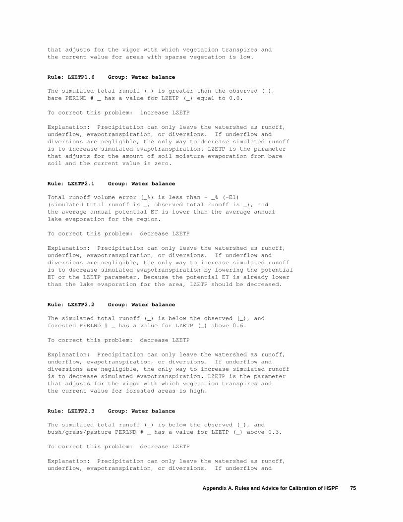
Appendix A. Rules and Advice for Calibration of HSPF 75
that adjusts for the vigor with which vegetation transpires andthe current value for areas with sparse vegetation is low.
Rule: LZETP1.6 Group: Water balance
The simulated total runoff (_) is greater than the observed (_),bare PERLND # _ has a value for LZETP (_) equal to 0.0.
To correct this problem: increase LZETP
Explanation: Precipitation can only leave the watershed as runoff,underflow, evapotranspiration, or diversions. If underflow anddiversions are negligible, the only way to decrease simulated runoffis to increase simulated evapotranspiration. LZETP is the parameterthat adjusts for the amount of soil moisture evaporation from baresoil and the current value is zero.
Rule: LZETP2.1 Group: Water balance
Total runoff volume error (_%) is less than - _% (-E1)(simulated total runoff is _, observed total runoff is _), andthe average annual potential ET is lower than the average annuallake evaporation for the region.
To correct this problem: decrease LZETP
Explanation: Precipitation can only leave the watershed as runoff,underflow, evapotranspiration, or diversions. If underflow anddiversions are negligible, the only way to increase simulated runoffis to decrease simulated evapotranspiration by lowering the potentialET or the LZETP parameter. Because the potential ET is already lowerthan the lake evaporation for the area, LZETP should be decreased.
Rule: LZETP2.2 Group: Water balance
The simulated total runoff (_) is below the observed (_), andforested PERLND # _ has a value for LZETP (_) above 0.6.
To correct this problem: decrease LZETP
Explanation: Precipitation can only leave the watershed as runoff,underflow, evapotranspiration, or diversions. If underflow anddiversions are negligible, the only way to increase simulated runoffis to decrease simulated evapotranspiration. LZETP is the parameterthat adjusts for the vigor with which vegetation transpires andthe current value for forested areas is high.
Rule: LZETP2.3 Group: Water balance
The simulated total runoff (_) is below the observed (_), andbush/grass/pasture PERLND # _ has a value for LZETP (_) above 0.3.
To correct this problem: decrease LZETP
Explanation: Precipitation can only leave the watershed as runoff,underflow, evapotranspiration, or diversions. If underflow and
76 Users Manual for an Expert System (HSPEXP) for Calibration of the Hydrological Simulation Program—Fortran
diversions are negligible, the only way to increase simulated runoffis to decrease simulated evapotranspiration. LZETP is the parameterthat adjusts for the vigor with which vegetation transpires andthe current value for bush/grass/pasture areas is high.
Rule: LZETP2.4 Group: Water balance
The simulated total runoff (_) is below the observed (_), androw-crop PERLND # _ has a value for LZETP (_) above 0.4.
To correct this problem: decrease LZETP
Explanation: Precipitation can only leave the watershed as runoff,underflow, evapotranspiration, or diversions. If underflow anddiversions are negligible, the only way to increase simulated runoffis to decrease simulated evapotranspiration. LZETP is the parameterthat adjusts for the vigor with which vegetation transpires andthe current value for row-crop areas is high.
Rule: LZETP2.5 Group: Water balance
The simulated total runoff (_) is below the observed (_), andsparse PERLND # _ has a value for LZETP (_) above 0.1.
To correct this problem: decrease LZETP
Explanation: Precipitation can only leave the watershed as runoff,underflow, evapotranspiration, or diversions. If underflow anddiversions are negligible, the only way to increase simulated runoffis to decrease simulated evapotranspiration. LZETP is the parameterthat adjusts for the vigor with which vegetation transpires andthe current value for sparsely vegetated areas is high.
Rule: LZETP2.6 Group: Water balance
The simulated total runoff (_) is below the observed (_), andbare PERLND # _ has a value for LZETP (_) above 0.0.
To correct this problem: decrease LZETP
Explanation: Precipitation can only leave the watershed as runoff,underflow, evapotranspiration, or diversions. If underflow anddiversions are negligible, the only way to increase simulated runoffis to decrease simulated evapotranspiration. LZETP is the parameterthat adjusts for the amount of soil moisture evaporation from baresoil and the current value is above zero.
Rule: DEPFR1.1 Group: Water balance
Total runoff volume error (_%) is greater than _% (E1)(simulated total runoff is _, observed total runoff is _), andthe difference between simulated and potential ET (_) is lessthan the difference between simulated and observed flow(_).
To correct this problem: increase DEEPFR
Appendix A. Rules and Advice for Calibration of HSPF 77
Explanation: Water budgets for watersheds must consider subsurfacelosses in addition to surface-water losses at the outlet andevapotranspiration losses. Assuming the estimate for potential ETis good, simulated ET cannot be increased very much. Thereforesubsurface losses must be increased and DEEPFR is the only parameterused to roughly estimate those losses.
Rule: DEPFR1.2 Group: Water balance
Total runoff volume error (_%) is greater than _% (E1)(simulated total runoff is _, observed total runoff is _), andthere could be recharge to deeper aquifers.
To correct this problem: increase DEEPFR
Explanation: Water budgets for watersheds must consider subsurfacelosses in addition to surface-water losses at the outlet andevapotranspiration losses. DEEPFR is the only parameter used toroughly estimate those losses and should be based on a ground-waterstudy of the area.
Rule: DEPFR2.1 Group: Water balance
Total runoff volume error (_%) is less than - _% (-E1)(simulated total runoff is _, observed total runoff is _), andthe simulated recharge to deeper aquifers could be too high, andPERLND # _ has a value for DEEPFR (_) greater than 0.0.
To correct this problem: decrease DEEPFR
Explanation: Water budgets for watersheds must consider subsurfacelosses in addition to surface-water losses at the outlet andevapotranspiration losses. DEEPFR is the only parameter used toroughly estimate those losses and should be based on a ground-waterstudy of the area.
Rule: LZSN1.1 Group: Water balance
Total runoff volume error (_%) is greater than _% (E1)(simulated total runoff is _, observed total runoff is _), andthe difference between simulated and potential ET (_) is greaterthan the difference between simulated and observed flow (_).
To correct this problem: increase LZSN
Explanation: If potential evapotranspiration and the transpirationfactor for vegetal cover (LZETP) are sufficiently high and thesubsurface losses are appropriate, then the only way to decreaseflow is to increase the storage capacity (LZSN) to provide greateropportunity for evapotranspiration.
Rule: LZSN1.2 Group: Water balance
The simulated total runoff (_) is greater than the observed (_), andLZSN times 1.5 is below the available water capacity of the soilfor the estimated rooting depth.
78 Users Manual for an Expert System (HSPEXP) for Calibration of the Hydrological Simulation Program—Fortran
To correct this problem: increase LZSN
Explanation: If potential evapotranspiration and the transpirationfactor for vegetal cover (LZETP) are sufficiently high and thesubsurface losses are appropriate, then the only way to decreaseflow is to increase the storage capacity (LZSN) to provide greateropportunity for evapotranspiration.
Rule: LZSN2.1 Group: Water balance
Total runoff volume error (_%) is less than - _% (-E1)(simulated total runoff is _, observed total runoff is _).
To correct this problem: decrease LZSN
Explanation: If potential evapotranspiration and the transpirationfactor for vegetal cover (LZETP) are sufficiently low and thesubsurface losses are appropriate, then the only way to increaseflow is to decrease the storage capacity (LZSN) to provide lessopportunity for evapotranspiration.
Rule: LZSN2.2 Group: Water balance
The simulated total runoff (_) is below the observed (_), andLZSN times 1.5 is above the available water capacity of the soilfor the estimated rooting depth.
To correct this problem: decrease LZSN
Explanation: If potential evapotranspiration and the transpirationfactor for vegetal cover (LZETP) are sufficiently low and thesubsurface losses are appropriate, then the only way to increaseflow is to decrease the storage capacity (LZSN) to provide lessopportunity for evapotranspiration.
Rule: INFLT3.1 Group: Water balance
Total runoff volume error (_%) is greater than _% (E1), andthe highest 10% of simulated daily mean flows (_) exceeds observed bymore than _ times _% (E9xE4), and the lowest 50% of simulateddaily flows (_) is lower than observed (_).
To correct this problem: increase INFILT
Explanation: The major effect of increased infiltration (INFILT) isto shift drainage from rapid response (surface runoff and interflow)to delayed response (base flow). Although INFILT does not have a strongdirect influence on water balance, it may be too far off for the otherparameters to correct for water-balance errors.
Rule: INFLT3.2 Group: Water balance
Total runoff volume error (_%) is greater than _% (E1), andthe highest 10% of simulated daily mean flows (_) exceedsobserved (_), and the lowest 50% of simulated daily mean flows (_)
Appendix A. Rules and Advice for Calibration of HSPF 79
is less than observed by more than _ times _% (E9xE3).
To correct this problem: increase INFILT
Explanation: The major effect of increased infiltration (INFILT) isto shift drainage from rapid response (surface runoff and interflow)to delayed response (base flow). Although INFILT does not have a strongdirect influence on water balance, it may be too far off for the otherparameters to correct for water-balance errors.
Rule: INFLT3.3 Group: Water balance
The simulated storm runoff volumes tend to be high, andthe subsequent simulated base flows are low.
To correct this problem: increase INFILT
Explanation: The major effect of increased infiltration (INFILT) isto shift drainage from rapid response (surface runoff and interflow)to delayed response (base flow). Although INFILT does not have a strongdirect influence on water balance, it may be too far off for the otherparameters to correct for water-balance errors.
Rule: INFLT4.1 Group: Water balance
Total runoff volume error (_%) is greater than _% (E1), andthe highest 10% of simulated daily mean flows (_) is below observedby more than _ times _% (E9xE4), and the lowest 50% simulatedflows (_) is greater than observed (_).
To correct this problem: decrease INFILT
Explanation: The major effect of decreased infiltration (INFILT) isto shift drainage from delayed response (base flow) to rapid response(surface runoff and interflow). Although INFILT does not have a strongdirect influence on water balance, it may be too far off for the otherparameters to correct for water-balance errors.
Rule: INFLT4.2 Group: Water balance
Total runoff volume error (_%) is greater than _% (E1), andthe highest 10% of simulated daily mean flows (_) is lower thanobserved (_), and the lowest 50% of simulated daily mean flows (_)exceeds the observed by more than _ times _% (E9xE3).
To correct this problem: decrease INFILT
Explanation: The major effect of decreased infiltration (INFILT) isto shift drainage from delayed response (base flow) to rapid response(surface runoff and interflow). Although INFILT does not have a strongdirect influence on water balance, it may be too far off for the otherparameters to correct for water-balance errors.
Rule: INFLT4.3 Group: Water balance
The simulated storm runoff volumes tend to be low, and
80 Users Manual for an Expert System (HSPEXP) for Calibration of the Hydrological Simulation Program—Fortran
the subsequent simulated base flows are high.
To correct this problem: decrease INFILT
Explanation: The major effect of decreased infiltration (INFILT) isto shift drainage from delayed response (base flow) to rapid response(surface runoff and interflow). Although INFILT does not have a strongdirect influence on water balance, it may be too far off for the otherparameters to correct for water-balance errors.
Rule: AGWRC1.1 Group: High-flow - low-flow distribution
The difference (_) between the average value of the daily recessionrate "Q(t)/Q(t-1)" during the base-flow period for the simulated flowand that for the observed flow is lower than - _ (-E2).
To correct this problem: increase AGWRC
Explanation: AGWRC is the fraction of yesterday's base flow that runsoff today. An increase will "flatten" the base-flow recession.
Rule: AGWRC1.2 Group: High-flow - low-flow distribution
The simulated winter base flow recedes faster than the observed winterbase flow, and the simulated summer base flow recedes faster than theobserved summer base flow.
To correct this problem: increase AGWRC
Explanation: AGWRC is the fraction of yesterday's base flow that runsoff today. An increase will "flatten" the base-flow recession.
Rule: AGWRC2.1 Group: High-flow - low-flow distribution
The difference (_) between the average value of the daily recessionrate "Q(t)/Q(t-1)" during the base-flow period for the simulated flowand that for the observed flow is greater than _ (E2), andPERLND # _ has a value for AGWRC (_) greater than or equal to 0.88.
To correct this problem: decrease AGWRC
Explanation: AGWRC is the fraction of yesterday's base flow that runsoff today. A decrease will "steepen" the base-flow recession. Thevalue for AGWRC is not too low.
Rule: AGWRC2.2 Group: High-flow - low-flow distribution
The simulated winter base flow recedes slower than the observed winterbase flow, and the simulated summer base flow recedes slower than theobserved summer base flow.
To correct this problem: decrease AGWRC
Explanation: AGWRC is the fraction of yesterday's base flow that runsoff today. A decrease will "steepen" the base-flow recession.
Appendix A. Rules and Advice for Calibration of HSPF 81
Rule: BSETP3.1 Group: High-flow - low-flow distribution
The difference (_) between the average value of the daily recessionrate "Q(t)/Q(t-1)" during the base-flow period for the simulated flowand that for the observed flow is greater than _ (E2), andPERLND # _ has a value for AGWRC (_) less than 0.88.
To correct this problem: increase BASETP
Explanation: The base-flow recession constant is so low that decreasingit more would make the flow like interflow. You should considerincreasing the effect of transpiration along the channels.
Rule: DEPFR3.1 Group: High-flow - low-flow distribution
The difference (_) between the average value of the daily recessionrate "Q(t)/Q(t-1)" during the base-flow period for the simulated flowand that for the observed flow is greater than _ (E2), andPERLND # _ has a value for AGWRC (_) less than 0.88.
To correct this problem: increase DEEPFR
Explanation: The base-flow recession constant is so low that decreasingit more would make the flow like interflow. You should consider sendingdrainage from the soil profile to deeper aquifers instead of base flow.
Rule: INFLT1.1 Group: High-flow - low-flow distribution
The highest 10% of simulated daily mean flows (_) is more than _% (E4)greater than observed (_), and the lowest 50% of simulated dailyflows (_) is less than observed (_).
To correct this problem: increase INFILT
Explanation: The major effect of increased infiltration (INFILT) isto shift drainage from rapid response (surface runoff and interflow)to delayed response (base flow).
Rule: INFLT1.2 Group: High-flow - low-flow distribution
The highest 10% of simulated daily mean flows (_) is greater thanobserved (_), and the lowest 50% of simulated daily mean flows (_)is more than _% (E3) less than observed (_).
To correct this problem: increase INFILT
Explanation: The major effect of increased infiltration (INFILT) isto shift drainage from rapid response (surface runoff and interflow)to delayed response (base flow).
Rule: INFLT1.3 Group: High-flow - low-flow distribution
The simulated storm runoff volumes tend to be high, andthe subsequent simulated base flows are low.
To correct this problem: increase INFILT
82 Users Manual for an Expert System (HSPEXP) for Calibration of the Hydrological Simulation Program—Fortran
Explanation: The major effect of increased infiltration (INFILT) isto shift drainage from rapid response (surface runoff and interflow)to delayed response (base flow).
Rule: INFLT2.1 Group: High-flow - low-flow distribution
The highest 10% of simulated daily mean flows (_) ismore than _% (E4) less than observed (_), and the lowest 50%of simulated mean daily flows (_) is greater than observed (_).
To correct this problem: decrease INFILT
Explanation: The major effect of decreased infiltration (INFILT) isto shift drainage from delayed response (base flow) to rapid response(surface runoff and interflow).
Rule: INFLT2.2 Group: High-flow - low-flow distribution
The highest 10% of simulated daily mean flows (_) is less thanobserved (_), and the lowest 50% of simulated daily mean flows (_)is more than _% (E3) greater than observed (_).
To correct this problem: decrease INFILT
Explanation: The major effect of decreased infiltration (INFILT) isto shift drainage from delayed response (base flow) to rapid response(surface runoff and interflow).
Rule: INFLT2.3 Group: High-flow - low-flow distribution
The simulated storm runoff volumes tend to be low, andthe subsequent simulated base flows are high.
To correct this problem: decrease INFILT
Explanation: The major effect of decreased infiltration (INFILT) isto shift drainage from delayed response (base flow) to rapid response(surface runoff and interflow).
Rule: LZSN3.1 Group: High-flow - low-flow distribution
The highest 10% of simulated daily mean flows (_)is less than _% (E4) less than observed (_), andthe lowest 50% of simulated daily mean flows (_)is more than _% (E3) greater than observed (_).
To correct this problem: increase LZSN
Explanation: If potential evapotranspiration and the transpiration factorfor vegetal cover (LZETP) are sufficiently high and the subsurface losses areappropriate, then the only way to decrease flow is to increase the storagecapacity (LZSN) to provide greater opportunity for evapotranspiration.
Appendix A. Rules and Advice for Calibration of HSPF 83
Rule: LZSN3.2 Group: High-flow - low-flow distribution
The highest 10% of simulated daily mean flows (_)is more than _% (E4) greater than observed (_), andthe lowest 50% of simulated daily mean flows (_)is less than _% (E3) less than observed (_).
To correct this problem: increase LZSN
Explanation: If potential evapotranspiration and the transpiration factorfor vegetal cover (LZETP) are sufficiently high and the subsurface losses areappropriate, then the only way to decrease flow is to increase the storagecapacity (LZSN) to provide greater opportunity for evapotranspiration.
Rule: LZSN3.3 Group: High-flow - low-flow distribution
The simulated total winter flow is the same or greater than observed,and the simulated total summer flow is lower than observed.
To correct this problem: increase LZSN
Explanation: If potential evapotranspiration and the transpiration factorfor vegetal cover (LZETP) are sufficiently high and the subsurface losses areappropriate, then the only way to decrease flow is to increase the storagecapacity (LZSN) to provide greater opportunity for evapotranspiration.
Rule: LZSN4.1 Group: High-flow - low-flow distribution
The highest 10% of simulated daily mean flows (_)is less than _% (E4) greater than observed (_), andthe lowest 50% of simulated daily mean flows (_)is more than _% (E3) less than observed (_).
To correct this problem: decrease LZSN
Explanation: If potential evapotranspiration and the transpiration factorfor vegetal cover (LZETP) are sufficiently low and the subsurface lossesare appropriate, then the only way to increase flow is to decrease thestorage capacity (LZSN) to provide less opportunity for evapotranspiration.
Rule: LZSN4.2 Group: High-flow - low-flow distribution
The highest 10% of simulated daily mean flows (_)is more than _% (E4) less than observed (_), andthe lowest 50% of simulated daily mean flows (_)is less than _% (E3) greater than observed (_).
To correct this problem: decrease LZSN
Explanation: If potential evapotranspiration and the transpiration factorfor vegetal cover (LZETP) are sufficiently low and the subsurface lossesare appropriate, then the only way to increase flow is to decrease thestorage capacity (LZSN) to provide less opportunity for evapotranspiration.
84 Users Manual for an Expert System (HSPEXP) for Calibration of the Hydrological Simulation Program—Fortran
Rule: LZSN4.3 Group: High-flow - low-flow distribution
The simulated total winter flowis the same or lower than observed, andthe simulated total summer flow is greater than observed.
To correct this problem: decrease LZSN
Explanation: If potential evapotranspiration and the transpiration factorfor vegetal cover (LZETP) are sufficiently low and the subsurface lossesare appropriate, then the only way to increase flow is to decrease thestorage capacity (LZSN) to provide less opportunity for evapotranspiration.
Rule: INFLT5.1 Group: Stormflow
Peak stormflow error (_%) is greater than _% (E5)(simulated peak stormflow is _, observed peak stormflow is _),and absolute value of the storm volume error (_%)is greater than _% (E5), andthe simulated storm volume (_) is greater than the observed (_).
To correct this problem: increase INFILT
Explanation: The major effect of increased infiltration (INFILT) isto shift drainage from rapid response (surface runoff and interflow)to delayed response (base flow), thus decreasing both simulated stormvolumes and simulated storm peaks.
Rule: INFLT6.1 Group: Stormflows
Peak stormflow error (_%) is less than - _% (-E5)(simulated peak stormflow is _, observed peak stormflow is _), andabsolute value of the storm volume error (_%)is greater than _% (E5), andthe simulated storm volume (_) is less than the observed (_).
To correct this problem: decrease INFILT
Explanation: The major effect of decreased infiltration (INFILT) isto shift drainage from delayed response (base flow) to rapid response(surface runoff and interflow), thus increasing both simulated stormvolumes and simulated storm peaks.
Rule: INTFW1.1 Group: Stormflows
Peak stormflow error (_%) is greater than _% (E5)(simulated peak stormflow is _, observed peak stormflow is _), andinterflow (_) is less than _ (E6) times the surface runoff (_), andabsolute value of the storm volume error (_%) is less than _% (E5)(simulated storm volume is _, observed storm volume is _).
To correct this problem: increase INTFW
Explanation: Runoff needs to be shifted from surface runoff tointerflow to put the water in a slower drainage category. If IRCis too low, however, interflow will respond like surface runoffand the increase in INTFW will have little effect.
Appendix A. Rules and Advice for Calibration of HSPF 85
Rule: INTFW1.2 Group: Stormflows
Peak stormflow error (_%) is greater than _% (E5)(simulated peak stormflow is _, observed peak stormflow is _), andinterflow (_) is less than _ (E6) times the surface runoff (_), andabsolute value of the storm volume error (_%)is greater than _% (E5), andthe simulated storm volume (_) is less than observed (_).
To correct this problem: increase INTFW
Explanation: Runoff needs to be shifted from surface runoff tointerflow to put the water in a slower drainage category. If IRCis too low, however, interflow will respond like surface runoffand the increase in INTFW will have little effect.
Rule: INTFW1.3 Group: Stormflows
Peak stormflow error (_%) is greater than _% (E5)(simulated peak stormflow is _, observed peak stormflow is _), andinterflow (_) is more than _ (E6) times the surface runoff (_), andabsolute value of the storm volume error (_%) is less than _% (E5)(simulated storm volume is _, observed storm volume is _), andPERLND # _ has values for IRC (_) > 0.6 and INTFW (_) < 7.5.
To correct this problem: increase INTFW
Explanation: Runoff needs to be shifted from surface runoff tointerflow to put the water in a slower drainage category. If IRCis too low, however, interflow will respond like surface runoffand the increase in INTFW will have little effect.
Rule: INTFW1.4 Group: Stormflows
Peak stormflow error (_%) is greater than _% (E5)(simulated peak stormflow is _, observed peak stormflow is _), andinterflow (_) is more than _ (E6) times the surface runoff (_), andabsolute value of the storm volume error (_%) is greater than _% (E5)(simulated storm volume is _, observed storm volume is _), andPERLND # _ has values for IRC (_) > 0.6 and INTFW (_) < 7.5.
To correct this problem: increase INTFW
Explanation: Runoff needs to be shifted from surface runoff tointerflow to put the water in a slower drainage category. If IRCis too low, however, interflow will respond like surface runoffand the increase in INTFW will have little effect.
Rule: INTFW1.5 Group: Stormflows
The simulated volume of runoff for major storms is about rightand the peaks are greater than observed, andPERLND # _ has a value for IRC (_) greater than 0.6.
To correct this problem: increase INTFW
Explanation: Runoff needs to be shifted from surface runoff to
86 Users Manual for an Expert System (HSPEXP) for Calibration of the Hydrological Simulation Program—Fortran
interflow to put the water in a slower drainage category. If IRCis too low, however, interflow will respond like surface runoffand the increase in INTFW will have little effect.
Rule: INTFW2.1 Group: Stormflows
Peak stormflow error (_%) is less than - _% (-E5)(simulated peak stormflow is _, observed peak stormflow is _), andinterflow (_) is less than _ (E6) times the surface runoff (_), andabsolute value of the storm volume error (_%) is less than _% (E5)(simulated storm volume is _, observed storm volume is _).
To correct this problem: decrease INTFW
Explanation: Runoff needs to be shifted from interflow to surfacerunoff to put the water in a faster drainage category. If IRCis too low, however, interflow will respond like surface runoffand the decrease in INTFW will have little effect on the peak.
Rule: INTFW2.2 Group: Stormflows
Peak stormflow error (_%) is less than - _% (-E5)(simulated peak stormflow is _, observed peak stormflow is _), andinterflow (_) is less than _ (E6) times the surface runoff (_), andabsolute value of the storm volume error (_%)is greater than _% (E5), andthe simulated storm volume (_) is greater than observed (_).
To correct this problem: decrease INTFW
Explanation: Runoff needs to be shifted from interflow to surfacerunoff to put the water in a faster drainage category. If IRCis too low, however, interflow will respond like surface runoffand the decrease in INTFW will have little effect on the peak.
Rule: INTFW2.3 Group: Stormflows
Peak stormflow error (_%) is less than - _% (-E5)(simulated peak stormflow is _, observed peak stormflow is _), andinterflow (_) is more than _ (E6) times the surface runoff (_), andabsolute value of the storm volume error (_%) is less than _% (E5)(simulated storm volume is _, observed storm volume is _), andPERLND # _ has values for IRC (_) < 0.4 and INTFW (_) > 1.0.
To correct this problem: decrease INTFW
Explanation: Runoff needs to be shifted from interflow to surfacerunoff to put the water in a faster drainage category. If IRCis too low, however, interflow will respond like surface runoffand the decrease in INTFW will have little effect on the peak.
Rule: INTFW2.4 Group: Stormflows
Peak stormflow error (_%) is less than - _% (-E5)(simulated peak stormflow is _, observed peak stormflow is _), andinterflow (_) is more than _ (E6) times the surface runoff (_), and
Appendix A. Rules and Advice for Calibration of HSPF 87
absolute value of the storm volume error (_%) is greater than _% (E5)(simulated storm volume is _, observed storm volume is _), andPERLND # _ has values for IRC (_) < 0.4 and INTFW (_) > 1.0.
To correct this problem: decrease INTFW
Explanation: Runoff needs to be shifted from interflow to surfacerunoff to put the water in a faster drainage category. If IRCis too low, however, interflow will respond like surface runoffand the decrease in INTFW will have little effect on the peak.
Rule: INTFW2.5 Group: Stormflows
The simulated volume of runoff for major storms is about rightand the peaks are lower than observed, andPERLND # _ has a value for IRC (_) less than 0.4.
To correct this problem: decrease INTFW
Explanation: Runoff needs to be shifted from interflow to surfacerunoff to put the water in a faster drainage category. If IRCis too low, however, interflow will respond like surface runoffand the decrease in INTFW will have little effect on the peak.
Rule: IRC1.1 Group: Stormflows
Peak stormflow error (_%) is less than - _% (-E5)(simulated peak stormflow is _, observed peak stormflow is _), andinterflow (_) is more than _ (E6) times the surface runoff (_), andabsolute value of the storm volume error (_%) is less than _% (E5)(simulated storm volume is _, observed storm volume is _), andPERLND # _ has a value for IRC (_) > 0.4, orPERLND # _ has values for IRC (_) > 0.3 and INTFW (_) <= to 1.0.
To correct this problem: decrease IRC
Explanation: Simulated peak flows for the storms are too low and mostof the storm runoff is interflow. Because IRC values are not too lowand the time required for interflow to drain following a storm isregulated with the parameter IRC, a decrease in IRC should increasepeak flows.
Rule: IRC1.2 Group: Stormflows
Peak stormflow error (_%) is less than - _% (-E5)(simulated peak stormflow is _, observed peak stormflow is _), andinterflow (_) is more than _ (E6) times the surface runoff (_), andabsolute value of the storm volume error (_%) is greater than _% (E5)(simulated storm volume is _, observed storm volume is _), andPERLND # _ has a value for IRC (_) > 0.4, orPERLND # _ has values for IRC (_) > 0.3 and INTFW (_) <= to 1.0.
To correct this problem: decrease IRC
Explanation: Simulated peak flows for the storms are too low and mostof the storm runoff is interflow. Because IRC values are not too lowand the time required for interflow to drain following a storm is
88 Users Manual for an Expert System (HSPEXP) for Calibration of the Hydrological Simulation Program—Fortran
regulated with the parameter IRC, a decrease in IRC should increasepeak flows.
Rule: IRC1.3 Group: Stormflows
The recession tails of simulated storm hydrographs recede slowerthan the recession tails of observed storm hydrographs, andthe simulated peak flow is lower than observed.
To correct this problem: decrease IRC
Explanation: Simulated peak flows for the storms are too low and adecrease in IRC should steepen the recession and increase peak flows.
Rule: IRC1.4 Group: Stormflows
The simulated volume of runoff for major storms is about rightand the peaks are lower than observed, andPERLND # _ has a value for IRC (_) greater than 0.4.
To correct this problem: decrease IRC
Explanation: Simulated peak flows for the storms are too low anda decrease in IRC should steepen the recession and increase peakflows without a change in volume.
Rule: IRC2.1 Group: Stormflows
Peak stormflow error (_%) is greater than _% (E5)(simulated peak stormflow is _, observed peak stormflow is _), andinterflow (_) is more than _ (E6) times the surface runoff (_), andabsolute value of the storm volume error (_%) is less than _% (E5)(simulated storm volume is _, observed storm volume is _), andPERLND # _ has a value for IRC (_) < 0.6, orPERLND # _ has values for IRC (_) < 0.7 and INTFW (_) >= 7.5.
To correct this problem: increase IRC
Explanation: Simulated peak flows for the storms are too high and mostof the storm runoff is interflow. Because IRC values are not too highand the time required for interflow to drain following a storm isregulated with the parameter IRC, an increase in IRC should decreasepeak flows.
Rule: IRC2.2 Group: Stormflows
Peak stormflow error (_%) is greater than _% (E5)(simulated peak stormflow is _, observed peak stormflow is _), andinterflow (_) is more than _ (E6) times the surface runoff (_), andabsolute value of the storm volume error (_%) is greater than _% (E5)(simulated storm volume is _, observed storm volume is _), andPERLND # _ has a value for IRC (_) < 0.6, orPERLND # _ has values for IRC (_) < 0.7 and INTFW (_) >= to 7.5.
To correct this problem: increase IRC
Appendix A. Rules and Advice for Calibration of HSPF 89
Explanation: Simulated peak flows for the storms are too high and mostof the storm runoff is interflow. Because IRC values are not too highand the time required for interflow to drain following a storm isregulated with the parameter IRC, an increase in IRC should decreasepeak flows.
Rule: IRC2.3 Group: Stormflows
The recession tails of the simulated storm hydrographs recede fasterthan the recession tails of the observed storm hydrographs, andthe simulated peak flow is greater than observed.
To correct this problem: increase IRC
Explanation: Simulated peak flows for the storms are too high and anincrease in IRC should flatten the recession and decrease peak flows.
Rule: IRC2.4 Group: Stormflows
The simulated volume of runoff for major storms is about rightand the peaks are greater than observed, andPERLND # _ has a value for IRC (_) less than 0.6.
To correct this problem: increase IRC
Explanation: Simulated peak flows for the storms are too high andan increase in IRC should flatten the recession and decrease peakflows without a change in volume.
Rule: KVARY1.1 Group: Seasonal
Simulated base flow during wet periods recedes more slowly than theobserved base flow, or simulated winter base flow recedes more slowlythan the observed winter base flow; and simulated summer base flowrecedes faster than the observed summer base flow, or simulated baseflow during dry periods recedes faster than the observed base flowduring dry periods.
To correct this problem: increase KVARY, decrease BASETP if there is channel or flood-plain vegetation, or decrease AGWETP if vegetation roots reach the ground-water table.
Explanation: KVARY has the effect of shifting base-flow drainage from drierperiods (no recharge) to shortly after wet periods (recent recharge). Itaccounts for greater contributing area immediately following a storm period.Evapotranspiration from the ground-water storage (AGWETP) or from the baseflow at the channel (BASETP) has a greater impact during the summer thanthe winter, which gives the effect of a steeper recession in the summer.
Rule: KVARY2.1 Group: Seasonal
Simulated base flow during wet periods recedes faster than the observedbase flow, or winter base flow recedes faster than the observed winter baseflow; and simulated summer base flow recedes more slowly than the observedsummer base flow, or simulated base flow during dry periods recedes moreslowly than the observed base flow during dry periods.
90 Users Manual for an Expert System (HSPEXP) for Calibration of the Hydrological Simulation Program—Fortran
To correct this problem: decrease KVARY, or increase BASETP if there is channel or flood-plain vegetation, or increase AGWETP if vegetation roots reach the ground-water table.
Explanation: KVARY has the effect of shifting base-flow drainage from drierperiods (no recharge) to shortly after wet periods (recent recharge). Itaccounts for greater contributing area immediately following a storm period.Evapotranspiration from the ground-water storage (AGWETP) or from the baseflow at the channel (BASETP) has a greater impact during the summer thanthe winter, which gives the effect of a steeper recession in the summer.
Rule: LZCEP1.1 Group: Seasonal
The summer flow error (_%) minus winter flow error (_%) is greaterthan _% (E7), and for PERLND # _ CEPSC and(or) LZETP is not inputas monthly values.
To correct this problem: input CEPSC and(or) LZETP as monthly values
Explanation: Row crops and hardwood forests are only effective forinterception and transpiration during the growing season and monthlyvalues of LZETP and CEPSC reflect that seasonal variation.
Rule: LZCEP1.2 Group: Seasonal
For PERLND # , the vegetation type is forest, mixed, or crop, andCEPSC and(or) LZETP is not input as monthly values.
To correct this problem: input CEPSC and(or) LZETP as monthly values
Explanation: Row crops and hardwood forests are only effective forinterception and transpiration during the growing season and monthlyvalues of LZETP and CEPSC reflect that seasonal variation.
Rule: UZSN1.1 Group: Seasonal
The average summer flow error (_%) minus the averagewinter flow error (_%) is less than - _% (-E7).
To correct this problem: decrease UZSN
Explanation: Surface storage in depressions and the upper fewinches of soil or forest litter remain near capacity in winterso that the value of this storage (UZSN) has minimal effect inwinter but a much larger influence in summer where losses forUZS are at or near the potential evapotranspiration.
Rule: UZSN1.2 Group: Seasonal
Storms with little antecedent rain (dry periods) are simulated low, andstorms with more antecedent rain (wet periods) are simulated high.
To correct this problem: decrease UZSN
Explanation: Surface storage in depressions and the upper few
Appendix A. Rules and Advice for Calibration of HSPF 91
inches of soil or forest litter remain near capacity in winterso that the value of this storage (UZSN) has minimal effect inwinter but a much larger influence in summer where losses forUZS are at or near the potential evapotranspiration.
Rule: UZSN2.1 Group: Seasonal
The average summer flow error (_%) minusthe average winter flow error (_%) is more than _% (E7).
To correct this problem: increase UZSN
Explanation: Surface storage in depressions and the upper fewinches of soil or forest litter remain near capacity in winterso that the value of this storage (UZSN) has minimal effect inwinter but a much larger influence in summer where losses forUZS are at or near the potential evapotranspiration.
Rule: UZSN2.2 Group: Seasonal
Storms with little antecedent rain (dry periods) are simulated high, andstorms with more antecedent rain (wet periods) are simulated low.
To correct this problem: increase UZSN
Explanation: Surface storage in depressions and the upper fewinches of soil or forest litter remain near capacity in winterso that the value of this storage (UZSN) has minimal effect inwinter but a much larger influence in summer where losses forUZS are at or near the potential evapotranspiration.
Rule: BSETP1.1 Group: Seasonal
Observed base flow increases in the fall and the simulated base flowdoes not, and there was no substantial rainfall.
To correct this problem: increase BASETP
Explanation: Although subsurface drainage to the channels takesplace during the summer, the vegetation around the channels istranspiring much of the water; as transpiration drops off in thefall, the flows will increase with no additional rainfall.
Rule: BSETP2.2 Group: Seasonal
Observed base flow decreases in the fall and the simulated baseflow does not, and there was no substantial rainfall, andPERLND # _ has a value for BASETP (_) greater than 0.0.
To correct this problem: decrease BASETP
Explanation: Although subsurface drainage to the channels takesplace during the summer, the vegetation around the channels istranspiring much of the water; as transpiration drops off inthe fall, the flows will increase with no additional rainfall.
92 Users Manual for an Expert System (HSPEXP) for Calibration of the Hydrological Simulation Program—Fortran
Rule: PRIMP1.1 Group: Seasonal
The difference (_%) between simulated and observedhigh flow during the summer months is greater than _% (E8)(simulated summer high flow is _, observed summer high flow is _).
To correct this problem: increase PERLND area and decrease IMPLND area by a corresponding amount.
Explanation: The most detectable effect from urban area(impervious area) on streamflow is an increase in stormflowsduring hot, dry periods usually in the summer.
Rule: PRIMP1.2 Group: Seasonal
The simulated high flow during summer months is greater than observed, andthere are urban areas in the watershed, andthe amount of IMPLND area might have been estimated high.
To correct this problem: increase PERLND area and decrease IMPLND area by a corresponding amount.
Explanation: The most detectable effect from urban area(impervious area) on streamflow is an increase in stormflowsduring hot, dry periods usually in the summer.
Rule: PRIMP2.1 Group: Seasonal
The difference (_%) between simulated and observedhigh flow during the summer months is less than - _% (-E8)(simulated summer high flow is _, observed summer high flow is _).
To correct this problem: decrease PERLND area and increase IMPLND area by a corresponding amount.
Explanation: The most detectable effect from urban area(impervious area) on streamflow is an increase in stormflowsduring hot, dry periods usually in the summer.
Rule: PRIMP2.2 Group: Seasonal
The simulated high flow during summer months is lower than observed, andthere are urban areas in the watershed, andthe amount of IMPLND area might have been estimated low.
To correct this problem: decrease PERLND area and increase IMPLND area by a corresponding amount.
Explanation: The most detectable effect from urban area(impervious area) on streamflow is an increase in stormflowsduring hot, dry periods usually in the summer.
Appendix B. User System Specifications File 93
APPENDIX B. USER SYSTEM SPECIFICATIONS FILE
The TERM.DAT file contains a number of parameters that define the configuration ofthe user's computer system and the user's preferences. All of these parameters default toa value that is considered most appropriate for the user’s computer system. Any numberof these defaults can be overridden by adding a TERM.DAT file to the directory wherethe program is being run. The first time the program needs any one of these parameters,they are read from the main message file. Then the user's TERM.DAT file is read, if itexists, and the parameters found replace the defaults from the message file. All of theparameters are saved for the duration of the run. Table B.1 lists the keyword, defaultvalue, allowable values, and the definition for each parameter. Table B.2 is theTERM.DAT parameters specifically for MS-DOS PC with color display only. Table B.3is the TERM.DAT parameters for graphics options. Table B.4 shows a TERM.DAT filethat modifies the background color of the graphics window from the default of black toa shade of purple. The keyword starts in column 1 and the value starts in column 8.
Many of the parameters depend on the implementation of GKS and give the user theopportunity to change or correct colors, line types, symbol types, symbol sizes,background color, text fonts, and graphics devices. With most implementations of GKS,text may be modified with the parameters GKPREC, GKSCFT, GKPRFT, GKPLFT,TXTEXF, and TXTCHS. Background color on color monitors can be changed usingparameters BCOLOR or BGRED, BGREEN, and BGBLUE. Symbol size can bemodified with the parameter SYSSIZ. Eight parameters are available to reset the defaultcode numbers for each of the curve specification, line type, symbol, color, and pattern.All code numbers should be available in the GKS documentation for workstations ordevice drivers.
Table B.1. TERM.DAT parameters for general use
Parameterkeyword
Defaultvalue
Allowablevalues Definition
TRMTYP PC PCVT100
Terminal type.
GRAPHS YES NOYES
Are GKS library and drivers available?
USRLEV 0 0 to 2 User experience level 0-lots, 2=none.
Table B.2. TERM.DAT parameters for color display (MS-DOS PC)
Parameterkeyword
Defaultvalue
Allowablevalues Definition
CLRFRM 15 0 to 15 Color of text for messages related to parameter input.CLRFRT 11 0 to 15 Color of titles and headers for full screen.CLRFRL 13 0 to 15 Color of limits for parameters.CLRFRE 4 0 to 15 Color for error messages.CLRFRC 14 0 to 15 Color for user input on command line.CLRFRP 7 0 to 15 Color for protected data values.CLRFRD 15 0 to 15 Color for data to be modified.CLRFRN 14 0 to 15 Color of data to be modified when currently none.CLRFRS 7 0 to 15 Standard color except for full screen.CLRBKO 2 0 to 15 Color of border.CLRBKB 1 0 to 15 Color of background for full screen.CLRBKS 0 0 to 15 Standard background color.CLRBKD 0 0 to 15 Color of background block for data to be modified.
TERM.DAT
94 Users Manual for an Expert System (HSPEXP) for Calibration of the Hydrological Simulation Program—Fortran
Table B.3. TERM.DAT parameters for graphics options
Default valuesParameterkeyword
DG PC UNIXAllowable
valuesDefinition
See the GKS implementation manual for your system or ask your GKS administrator for a list of supported codes.GKSDIS 4107 any GKS code number for workstation type for display terminal.GKSPRT 102 any GKS code number for workstation type for printer device.GKSPLT 9012 any GKS code number for workstation type for pen plotter.GKSMET 9005 any GKS code number for metafile.GKSDSP 102 any DISSPLA metafile code number.GKPREC CHAR STRING
CHARSTROKE
Text precision, see GKS manual for computer system and devicetype.
GKSCFT 1 -9999 to 9999 Text font for screen.GKPRFT 1 -9999 to 9999 Text font for printer.GKPLFT 1 -9999 to 9999 Text font for plotter.LSOLID 1 -9999 to 9999 Code for solid line.LDASH 2 -9999 to 9999 Code for dashed line.LDOT 3 -9999 to 9999 Code for dotted line.
LMIXED 4 -9999 to 9999 Code for dot dashed line.1LUSER 1 -9999 to 9999 Extra line type code.2LUSER 1 -9999 to 9999 Extra line type code.3LUSER 1 -9999 to 9999 Extra line type code.4LUSER 1 -9999 to 9999 Extra line type code.CBLACK 1 -9999 to 9999 Code for black.CWHITE 2 -9999 to 9999 Code for white.CRED 3 -9999 to 9999 Code for red.CGREEN 4 -9999 to 9999 Code for green.CBLUE 5 -9999 to 9999 Code for blue.CCYAN 6 -9999 to 9999 Code for cyan.CMAGNT 7 -9999 to 9999 Code for magenta.CYELLOW 8 -9999 to 9999 Code for yellow.CDOT 1 -9999 to 9999 Symbol code for dot.CPLUS 2 -9999 to 9999 Symbol code for plus.CSTAR 3 -9999 to 9999 Symbol code for star.CZERO 4 -9999 to 9999 Symbol code for circle.CX 5 -9999 to 9999 Symbol code for X.1SUSER 1 -9999 to 9999 Extra symbol code.2SUSER 1 -9999 to 9999 Extra symbol code.PSOLID 2 -9999 to 9999 Code for solid fill area.PHORIZ 3 -9999 to 9999 Code for horizontal fill area.PVERT 4 -9999 to 9999 Code for vertical fill area.PDIAG 5 -9999 to 9999 Code for diagonal fill area.1PUSER 1 -9999 to 9999 Extra fill code.2PUSER 1 -9999 to 9999 Extra fill code.3PUSER 1 -9999 to 9999 Extra fill code.4PUSER 1 -9999 to 9999 Extra fill code.SYMSIZ 100 1 to 10000 Symbol size ratio in hundredths.TXTEXF 0 0 to 200 Text expansion factor in hundredths.TXTCHS 0 0 to 200 Text character spacing in hundredths.
Appendix B. User System Specifications File 95
BCOLOR BLACK BLACKWHITEOTHER
Background color.
BGRED 0 0 to 100 Percent red for background if BCOLOR=OTHER.BGREEN 0 0 to 100 Percent green for background if BCOLOR=OTHER.BGBLUE 0 0 to 100 Percent blue for background if BCOLOR=OTHER.
Table B.4. Example TERM.DAT
File contentsDescription
(Note: description is not part of file)
BCOLOR OTHER Background color is other
BGBLUE 60 Percent blue is 60
BGRED 40 Percent red is 40
BGREEN 0 Percent green is 0
Table B.3. TERM.DAT parameters for graphics options--Continued
Default valuesParameterkeyword
DG PC UNIXAllowable
valuesDefinition

96 Users Manual for an Expert System (HSPEXP) for Calibration of the Hydrological Simulation Program—Fortran
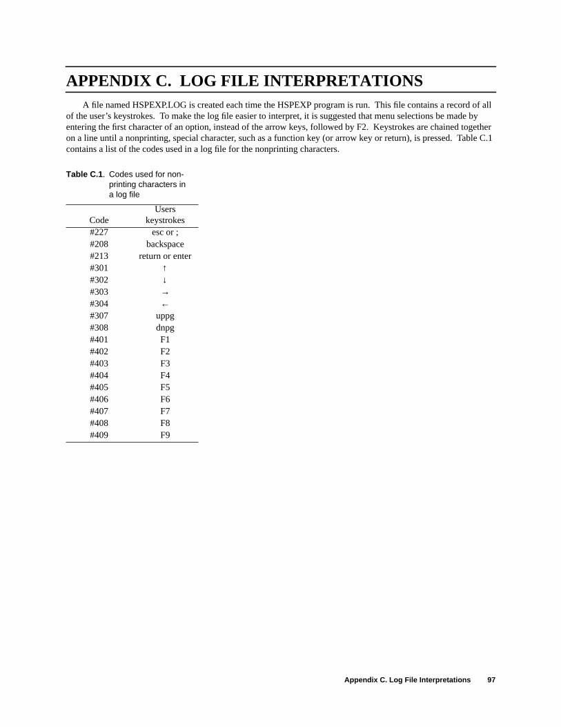
Appendix C. Log File Interpretations 97
APPENDIX C. LOG FILE INTERPRETATIONSA file named HSPEXP.LOG is created each time the HSPEXP program is run. This file contains a record of all
of the user’s keystrokes. To make the log file easier to interpret, it is suggested that menu selections be made byentering the first character of an option, instead of the arrow keys, followed by F2. Keystrokes are chained togetheron a line until a nonprinting, special character, such as a function key (or arrow key or return), is pressed. Table C.1contains a list of the codes used in a log file for the nonprinting characters.
Table C.1 . Codes used for non-printing characters ina log file
CodeUsers
keystrokes#227 esc or ;#208 backspace#213 return or enter#301 ↑#302 ↓#303 →#304 ←#307 uppg#308 dnpg#401 F1#402 F2#403 F3#404 F4#405 F5#406 F6#407 F7#408 F8#409 F9

98 Users Manual for an Expert System (HSPEXP) for Calibration of the Hydrological Simulation Program—Fortran
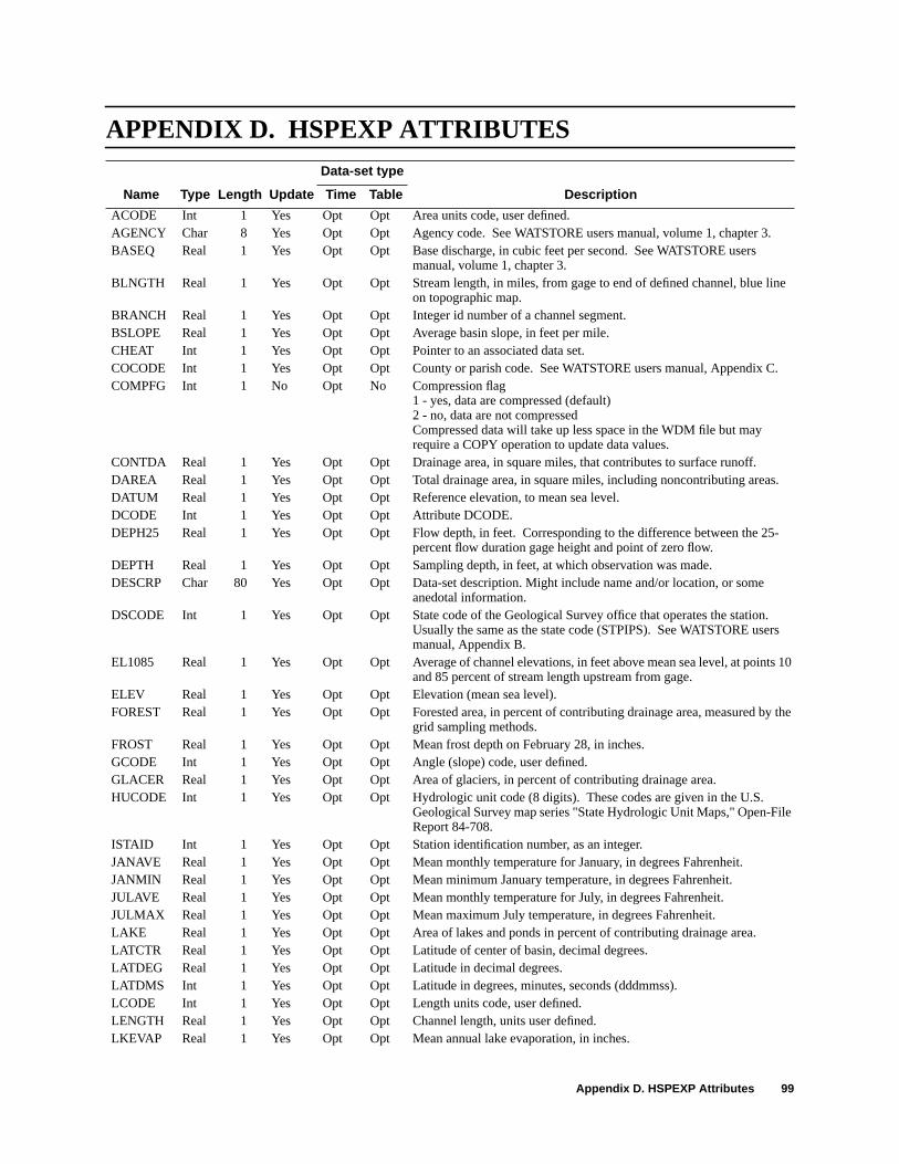
Appendix D. HSPEXP Attributes 99
APPENDIX D. HSPEXP ATTRIBUTESData-set type
Name Type Length Update Time Table Description
ACODE Int 1 Yes Opt Opt Area units code, user defined.AGENCY Char 8 Yes Opt Opt Agency code. See WATSTORE users manual, volume 1, chapter 3.BASEQ Real 1 Yes Opt Opt Base discharge, in cubic feet per second. See WATSTORE users
manual, volume 1, chapter 3.BLNGTH Real 1 Yes Opt Opt Stream length, in miles, from gage to end of defined channel, blue line
on topographic map.BRANCH Real 1 Yes Opt Opt Integer id number of a channel segment.BSLOPE Real 1 Yes Opt Opt Average basin slope, in feet per mile.CHEAT Int 1 Yes Opt Opt Pointer to an associated data set.COCODE Int 1 Yes Opt Opt County or parish code. See WATSTORE users manual, Appendix C.COMPFG Int 1 No Opt No Compression flag
1 - yes, data are compressed (default)2 - no, data are not compressedCompressed data will take up less space in the WDM file but mayrequire a COPY operation to update data values.
CONTDA Real 1 Yes Opt Opt Drainage area, in square miles, that contributes to surface runoff.DAREA Real 1 Yes Opt Opt Total drainage area, in square miles, including noncontributing areas.DATUM Real 1 Yes Opt Opt Reference elevation, to mean sea level.DCODE Int 1 Yes Opt Opt Attribute DCODE.DEPH25 Real 1 Yes Opt Opt Flow depth, in feet. Corresponding to the difference between the 25-
percent flow duration gage height and point of zero flow.DEPTH Real 1 Yes Opt Opt Sampling depth, in feet, at which observation was made.DESCRP Char 80 Yes Opt Opt Data-set description. Might include name and/or location, or some
anedotal information.DSCODE Int 1 Yes Opt Opt State code of the Geological Survey office that operates the station.
Usually the same as the state code (STPIPS). See WATSTORE usersmanual, Appendix B.
EL1085 Real 1 Yes Opt Opt Average of channel elevations, in feet above mean sea level, at points 10and 85 percent of stream length upstream from gage.
ELEV Real 1 Yes Opt Opt Elevation (mean sea level).FOREST Real 1 Yes Opt Opt Forested area, in percent of contributing drainage area, measured by the
grid sampling methods.FROST Real 1 Yes Opt Opt Mean frost depth on February 28, in inches.GCODE Int 1 Yes Opt Opt Angle (slope) code, user defined.GLACER Real 1 Yes Opt Opt Area of glaciers, in percent of contributing drainage area.HUCODE Int 1 Yes Opt Opt Hydrologic unit code (8 digits). These codes are given in the U.S.
Geological Survey map series "State Hydrologic Unit Maps," Open-FileReport 84-708.
ISTAID Int 1 Yes Opt Opt Station identification number, as an integer.JANAVE Real 1 Yes Opt Opt Mean monthly temperature for January, in degrees Fahrenheit.JANMIN Real 1 Yes Opt Opt Mean minimum January temperature, in degrees Fahrenheit.JULAVE Real 1 Yes Opt Opt Mean monthly temperature for July, in degrees Fahrenheit.JULMAX Real 1 Yes Opt Opt Mean maximum July temperature, in degrees Fahrenheit.LAKE Real 1 Yes Opt Opt Area of lakes and ponds in percent of contributing drainage area.LATCTR Real 1 Yes Opt Opt Latitude of center of basin, decimal degrees.LATDEG Real 1 Yes Opt Opt Latitude in decimal degrees.LATDMS Int 1 Yes Opt Opt Latitude in degrees, minutes, seconds (dddmmss).LCODE Int 1 Yes Opt Opt Length units code, user defined.LENGTH Real 1 Yes Opt Opt Channel length, units user defined.LKEVAP Real 1 Yes Opt Opt Mean annual lake evaporation, in inches.
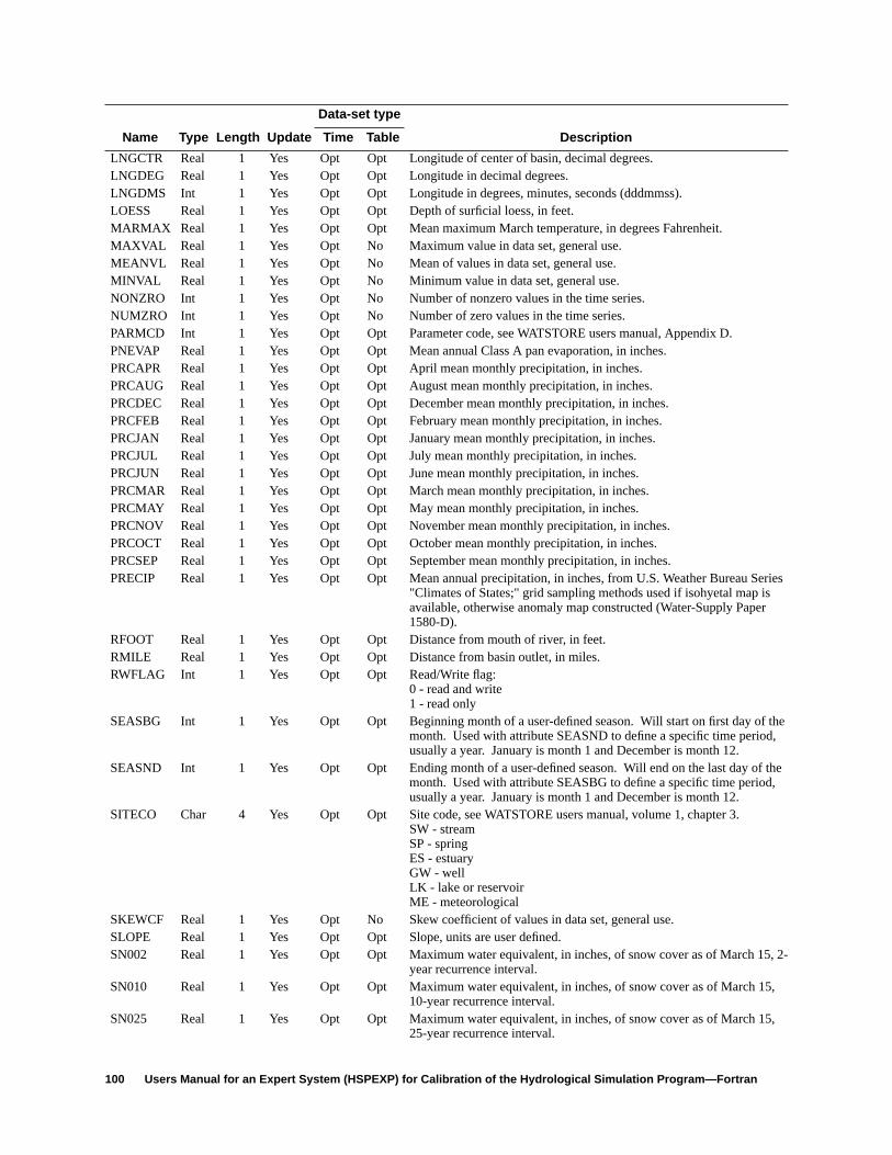
100 Users Manual for an Expert System (HSPEXP) for Calibration of the Hydrological Simulation Program—Fortran
LNGCTR Real 1 Yes Opt Opt Longitude of center of basin, decimal degrees.LNGDEG Real 1 Yes Opt Opt Longitude in decimal degrees.LNGDMS Int 1 Yes Opt Opt Longitude in degrees, minutes, seconds (dddmmss).LOESS Real 1 Yes Opt Opt Depth of surficial loess, in feet.MARMAX Real 1 Yes Opt Opt Mean maximum March temperature, in degrees Fahrenheit.MAXVAL Real 1 Yes Opt No Maximum value in data set, general use.MEANVL Real 1 Yes Opt No Mean of values in data set, general use.MINVAL Real 1 Yes Opt No Minimum value in data set, general use.NONZRO Int 1 Yes Opt No Number of nonzero values in the time series.NUMZRO Int 1 Yes Opt No Number of zero values in the time series.PARMCD Int 1 Yes Opt Opt Parameter code, see WATSTORE users manual, Appendix D.PNEVAP Real 1 Yes Opt Opt Mean annual Class A pan evaporation, in inches.PRCAPR Real 1 Yes Opt Opt April mean monthly precipitation, in inches.PRCAUG Real 1 Yes Opt Opt August mean monthly precipitation, in inches.PRCDEC Real 1 Yes Opt Opt December mean monthly precipitation, in inches.PRCFEB Real 1 Yes Opt Opt February mean monthly precipitation, in inches.PRCJAN Real 1 Yes Opt Opt January mean monthly precipitation, in inches.PRCJUL Real 1 Yes Opt Opt July mean monthly precipitation, in inches.PRCJUN Real 1 Yes Opt Opt June mean monthly precipitation, in inches.PRCMAR Real 1 Yes Opt Opt March mean monthly precipitation, in inches.PRCMAY Real 1 Yes Opt Opt May mean monthly precipitation, in inches.PRCNOV Real 1 Yes Opt Opt November mean monthly precipitation, in inches.PRCOCT Real 1 Yes Opt Opt October mean monthly precipitation, in inches.PRCSEP Real 1 Yes Opt Opt September mean monthly precipitation, in inches.PRECIP Real 1 Yes Opt Opt Mean annual precipitation, in inches, from U.S. Weather Bureau Series
"Climates of States;" grid sampling methods used if isohyetal map isavailable, otherwise anomaly map constructed (Water-Supply Paper1580-D).
RFOOT Real 1 Yes Opt Opt Distance from mouth of river, in feet.RMILE Real 1 Yes Opt Opt Distance from basin outlet, in miles.RWFLAG Int 1 Yes Opt Opt Read/Write flag:
0 - read and write1 - read only
SEASBG Int 1 Yes Opt Opt Beginning month of a user-defined season. Will start on first day of themonth. Used with attribute SEASND to define a specific time period,usually a year. January is month 1 and December is month 12.
SEASND Int 1 Yes Opt Opt Ending month of a user-defined season. Will end on the last day of themonth. Used with attribute SEASBG to define a specific time period,usually a year. January is month 1 and December is month 12.
SITECO Char 4 Yes Opt Opt Site code, see WATSTORE users manual, volume 1, chapter 3.SW - streamSP - springES - estuaryGW - wellLK - lake or reservoirME - meteorological
SKEWCF Real 1 Yes Opt No Skew coefficient of values in data set, general use.SLOPE Real 1 Yes Opt Opt Slope, units are user defined.SN002 Real 1 Yes Opt Opt Maximum water equivalent, in inches, of snow cover as of March 15, 2-
year recurrence interval.SN010 Real 1 Yes Opt Opt Maximum water equivalent, in inches, of snow cover as of March 15,
10-year recurrence interval.SN025 Real 1 Yes Opt Opt Maximum water equivalent, in inches, of snow cover as of March 15,
25-year recurrence interval.
Data-set type
Name Type Length Update Time Table Description
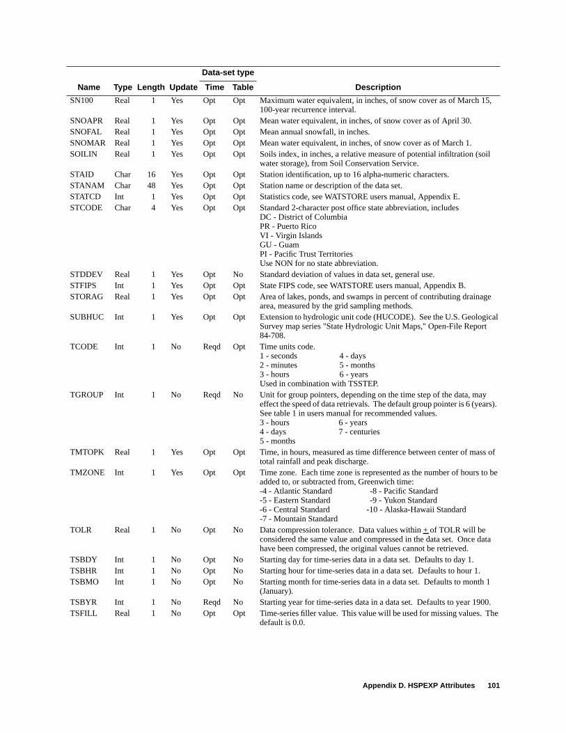
Appendix D. HSPEXP Attributes 101
SN100 Real 1 Yes Opt Opt Maximum water equivalent, in inches, of snow cover as of March 15,100-year recurrence interval.
SNOAPR Real 1 Yes Opt Opt Mean water equivalent, in inches, of snow cover as of April 30.SNOFAL Real 1 Yes Opt Opt Mean annual snowfall, in inches.SNOMAR Real 1 Yes Opt Opt Mean water equivalent, in inches, of snow cover as of March 1.SOILIN Real 1 Yes Opt Opt Soils index, in inches, a relative measure of potential infiltration (soil
water storage), from Soil Conservation Service.STAID Char 16 Yes Opt Opt Station identification, up to 16 alpha-numeric characters.STANAM Char 48 Yes Opt Opt Station name or description of the data set.STATCD Int 1 Yes Opt Opt Statistics code, see WATSTORE users manual, Appendix E.STCODE Char 4 Yes Opt Opt Standard 2-character post office state abbreviation, includes
DC - District of ColumbiaPR - Puerto RicoVI - Virgin IslandsGU - GuamPI - Pacific Trust TerritoriesUse NON for no state abbreviation.
STDDEV Real 1 Yes Opt No Standard deviation of values in data set, general use.STFIPS Int 1 Yes Opt Opt State FIPS code, see WATSTORE users manual, Appendix B.STORAG Real 1 Yes Opt Opt Area of lakes, ponds, and swamps in percent of contributing drainage
area, measured by the grid sampling methods.SUBHUC Int 1 Yes Opt Opt Extension to hydrologic unit code (HUCODE). See the U.S. Geological
Survey map series "State Hydrologic Unit Maps," Open-File Report84-708.
TCODE Int 1 No Reqd Opt Time units code.1 - seconds 4 - days2 - minutes 5 - months3 - hours 6 - yearsUsed in combination with TSSTEP.
TGROUP Int 1 No Reqd No Unit for group pointers, depending on the time step of the data, mayeffect the speed of data retrievals. The default group pointer is 6 (years).See table 1 in users manual for recommended values.3 - hours 6 - years4 - days 7 - centuries5 - months
TMTOPK Real 1 Yes Opt Opt Time, in hours, measured as time difference between center of mass oftotal rainfall and peak discharge.
TMZONE Int 1 Yes Opt Opt Time zone. Each time zone is represented as the number of hours to beadded to, or subtracted from, Greenwich time:-4 - Atlantic Standard -8 - Pacific Standard-5 - Eastern Standard -9 - Yukon Standard-6 - Central Standard -10 - Alaska-Hawaii Standard-7 - Mountain Standard
TOLR Real 1 No Opt No Data compression tolerance. Data values within+ of TOLR will beconsidered the same value and compressed in the data set. Once datahave been compressed, the original values cannot be retrieved.
TSBDY Int 1 No Opt No Starting day for time-series data in a data set. Defaults to day 1.TSBHR Int 1 No Opt No Starting hour for time-series data in a data set. Defaults to hour 1.TSBMO Int 1 No Opt No Starting month for time-series data in a data set. Defaults to month 1
(January).TSBYR Int 1 No Reqd No Starting year for time-series data in a data set. Defaults to year 1900.TSFILL Real 1 No Opt Opt Time-series filler value. This value will be used for missing values. The
default is 0.0.
Data-set type
Name Type Length Update Time Table Description
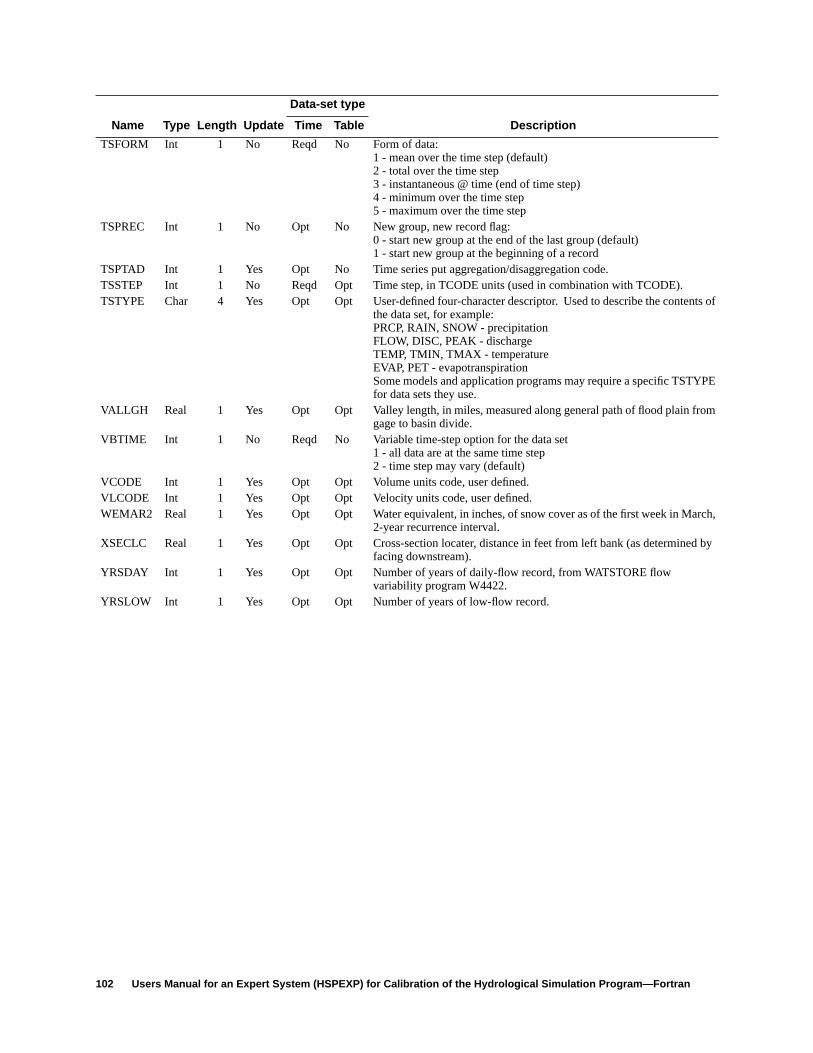
102 Users Manual for an Expert System (HSPEXP) for Calibration of the Hydrological Simulation Program—Fortran
TSFORM Int 1 No Reqd No Form of data:1 - mean over the time step (default)2 - total over the time step3 - instantaneous @ time (end of time step)4 - minimum over the time step5 - maximum over the time step
TSPREC Int 1 No Opt No New group, new record flag:0 - start new group at the end of the last group (default)1 - start new group at the beginning of a record
TSPTAD Int 1 Yes Opt No Time series put aggregation/disaggregation code.TSSTEP Int 1 No Reqd Opt Time step, in TCODE units (used in combination with TCODE).TSTYPE Char 4 Yes Opt Opt User-defined four-character descriptor. Used to describe the contents of
the data set, for example:PRCP, RAIN, SNOW - precipitationFLOW, DISC, PEAK - dischargeTEMP, TMIN, TMAX - temperatureEVAP, PET - evapotranspirationSome models and application programs may require a specific TSTYPEfor data sets they use.
VALLGH Real 1 Yes Opt Opt Valley length, in miles, measured along general path of flood plain fromgage to basin divide.
VBTIME Int 1 No Reqd No Variable time-step option for the data set1 - all data are at the same time step2 - time step may vary (default)
VCODE Int 1 Yes Opt Opt Volume units code, user defined.VLCODE Int 1 Yes Opt Opt Velocity units code, user defined.WEMAR2 Real 1 Yes Opt Opt Water equivalent, in inches, of snow cover as of the first week in March,
2-year recurrence interval.XSECLC Real 1 Yes Opt Opt Cross-section locater, distance in feet from left bank (as determined by
facing downstream).YRSDAY Int 1 Yes Opt Opt Number of years of daily-flow record, from WATSTORE flow
variability program W4422.YRSLOW Int 1 Yes Opt Opt Number of years of low-flow record.
Data-set type
Name Type Length Update Time Table Description