user’s guide to parssim1: the parallel subsurface...
TRANSCRIPT

User’s Guide to Parssim1:The Parallel SubsurfaceSimulator, Single Phase
Version: Parssim1 v. 2.1May 1998
(Minor updates to February 21, 2006)
Todd Arbogast
Code Management:The Center for Subsurface Modeling
Mary F. Wheeler, director, Steven Bryant, associate director,Todd Arbogast, and Clint Dawson
Texas Institute for Computational and Applied MathematicsThe University of Texas at AustinAustin, Texas 78712
[email protected], [email protected],[email protected], [email protected]
Copyright: No portion of this document or program may be reproduced, transmitted or otherwisecopied without prior written permission of the Center for Subsurface Modeling (CSM), TexasInstitute for Computational and Applied Mathematics, The University of Texas at Austin, exceptfor the internal use of the CSM. The authors make no representations or warranties about thecorrectness of any portion of the program code, supplementary codes, or associated documentation,nor about the suitability of this program for any purpose, and is in no way liable for any damagesresulting from its use or misuse.
1
Table of Contents
1 Brief Summary 5
2 Governing Equations and Numerical Methods 62.1 Notation . . . . . . . . . . . . . . . . . . . . . . . . . . . . . . . . . . . . . . . . . . . . 62.2 Flow . . . . . . . . . . . . . . . . . . . . . . . . . . . . . . . . . . . . . . . . . . . . . . . 6
2.2.1 Viscosity Quarter Power Mixing Rule . . . . . . . . . . . . . . . . . . . . . . . . 72.2.2 Numerical Solution . . . . . . . . . . . . . . . . . . . . . . . . . . . . . . . . . . 7
2.3 Transport . . . . . . . . . . . . . . . . . . . . . . . . . . . . . . . . . . . . . . . . . . . . 72.3.1 Diffusion/Dispersion Tensor . . . . . . . . . . . . . . . . . . . . . . . . . . . . . 82.3.2 Linear Sorption Model . . . . . . . . . . . . . . . . . . . . . . . . . . . . . . . . 82.3.3 Numerical Solution . . . . . . . . . . . . . . . . . . . . . . . . . . . . . . . . . . 9
2.4 Chemistry Overview . . . . . . . . . . . . . . . . . . . . . . . . . . . . . . . . . . . . . . 102.4.1 Specialized Chemistry . . . . . . . . . . . . . . . . . . . . . . . . . . . . . . . . 102.4.2 General Chemistry Package . . . . . . . . . . . . . . . . . . . . . . . . . . . . . 112.4.3 Numerical Solution . . . . . . . . . . . . . . . . . . . . . . . . . . . . . . . . . . 11
2.5 General Chemistry . . . . . . . . . . . . . . . . . . . . . . . . . . . . . . . . . . . . . . . 112.5.1 Thermodynamics . . . . . . . . . . . . . . . . . . . . . . . . . . . . . . . . . . . 112.5.2 Kinetic reactions and their rate-laws . . . . . . . . . . . . . . . . . . . . . . . . 142.5.3 Numerical parameters . . . . . . . . . . . . . . . . . . . . . . . . . . . . . . . . 15
2.6 Radionuclide Decay . . . . . . . . . . . . . . . . . . . . . . . . . . . . . . . . . . . . . . 17
3 Program Name and Command Line Arguments 18
4 General Input File Syntax and Physical Units 194.1 White-space . . . . . . . . . . . . . . . . . . . . . . . . . . . . . . . . . . . . . . . . . . 194.2 Commands . . . . . . . . . . . . . . . . . . . . . . . . . . . . . . . . . . . . . . . . . . . 194.3 Comments . . . . . . . . . . . . . . . . . . . . . . . . . . . . . . . . . . . . . . . . . . . 204.4 Sectional Units . . . . . . . . . . . . . . . . . . . . . . . . . . . . . . . . . . . . . . . . . 204.5 List Delimiters . . . . . . . . . . . . . . . . . . . . . . . . . . . . . . . . . . . . . . . . . 204.6 Key-words . . . . . . . . . . . . . . . . . . . . . . . . . . . . . . . . . . . . . . . . . . . 214.7 Data Items . . . . . . . . . . . . . . . . . . . . . . . . . . . . . . . . . . . . . . . . . . . 21
4.7.1 Physical Units . . . . . . . . . . . . . . . . . . . . . . . . . . . . . . . . . . . . . 214.7.2 Data Blocks and the Repetition Symbol . . . . . . . . . . . . . . . . . . . . . . 224.7.3 Grid Arrays: Constant, Nearly Constant, and Fully Specified . . . . . . . . . . 22
5 The Input Data File(s) 255.1 General Information . . . . . . . . . . . . . . . . . . . . . . . . . . . . . . . . . . . . . . 255.2 Algorithm Solution Parameters . . . . . . . . . . . . . . . . . . . . . . . . . . . . . . . . 26
5.2.1 Flow . . . . . . . . . . . . . . . . . . . . . . . . . . . . . . . . . . . . . . . . . . 27
2
5.2.2 Transport . . . . . . . . . . . . . . . . . . . . . . . . . . . . . . . . . . . . . . . 275.2.3 Chemistry . . . . . . . . . . . . . . . . . . . . . . . . . . . . . . . . . . . . . . . 28
5.3 Time Control . . . . . . . . . . . . . . . . . . . . . . . . . . . . . . . . . . . . . . . . . . 305.3.1 Flow . . . . . . . . . . . . . . . . . . . . . . . . . . . . . . . . . . . . . . . . . . 305.3.2 Transport . . . . . . . . . . . . . . . . . . . . . . . . . . . . . . . . . . . . . . . 30
5.4 Spatial Grid . . . . . . . . . . . . . . . . . . . . . . . . . . . . . . . . . . . . . . . . . . 315.4.1 Uniform Rectangular Grid . . . . . . . . . . . . . . . . . . . . . . . . . . . . . . 315.4.2 Nonuniform Rectangular Grid . . . . . . . . . . . . . . . . . . . . . . . . . . . . 325.4.3 An XY-rectangular, Z-variable Grid . . . . . . . . . . . . . . . . . . . . . . . . 325.4.4 A Fully Logically Rectangular Grid . . . . . . . . . . . . . . . . . . . . . . . . . 32
5.5 Porous Medium Material Properties . . . . . . . . . . . . . . . . . . . . . . . . . . . . . 335.5.1 Permeabilities (or Conductivities) . . . . . . . . . . . . . . . . . . . . . . . . . . 335.5.2 Dispersion . . . . . . . . . . . . . . . . . . . . . . . . . . . . . . . . . . . . . . . 355.5.3 Linear Sorption/Retardation . . . . . . . . . . . . . . . . . . . . . . . . . . . . 35
5.6 Phase Properties . . . . . . . . . . . . . . . . . . . . . . . . . . . . . . . . . . . . . . . . 365.6.1 Phase Description . . . . . . . . . . . . . . . . . . . . . . . . . . . . . . . . . . . 36
5.7 General Chemistry Properties . . . . . . . . . . . . . . . . . . . . . . . . . . . . . . . . 365.8 Chemical Species Properties . . . . . . . . . . . . . . . . . . . . . . . . . . . . . . . . . 37
5.8.1 Species Description . . . . . . . . . . . . . . . . . . . . . . . . . . . . . . . . . . 375.9 Miscible Displacement . . . . . . . . . . . . . . . . . . . . . . . . . . . . . . . . . . . . . 39
5.9.1 Quarter Power Mixing Rule . . . . . . . . . . . . . . . . . . . . . . . . . . . . . 395.10 Radionuclide Decay . . . . . . . . . . . . . . . . . . . . . . . . . . . . . . . . . . . . . . 405.11 Specialized Reactions . . . . . . . . . . . . . . . . . . . . . . . . . . . . . . . . . . . . . 405.12 Initial Conditions . . . . . . . . . . . . . . . . . . . . . . . . . . . . . . . . . . . . . . . 41
5.12.1 Flow . . . . . . . . . . . . . . . . . . . . . . . . . . . . . . . . . . . . . . . . . . 415.12.2 Transport . . . . . . . . . . . . . . . . . . . . . . . . . . . . . . . . . . . . . . . 42
5.13 Boundary Conditions . . . . . . . . . . . . . . . . . . . . . . . . . . . . . . . . . . . . . 425.13.1 Boundary Region Specification . . . . . . . . . . . . . . . . . . . . . . . . . . . 43
5.14 Well Specification . . . . . . . . . . . . . . . . . . . . . . . . . . . . . . . . . . . . . . . 455.14.1 Single Well Description . . . . . . . . . . . . . . . . . . . . . . . . . . . . . . . . 45
5.15 Leaking Source Specification . . . . . . . . . . . . . . . . . . . . . . . . . . . . . . . . . 475.15.1 Single Leak Description . . . . . . . . . . . . . . . . . . . . . . . . . . . . . . . 47
5.16 Output . . . . . . . . . . . . . . . . . . . . . . . . . . . . . . . . . . . . . . . . . . . . . 485.16.1 Flow . . . . . . . . . . . . . . . . . . . . . . . . . . . . . . . . . . . . . . . . . . 495.16.2 Transport . . . . . . . . . . . . . . . . . . . . . . . . . . . . . . . . . . . . . . . 49
6 Input Error Messages 52
7 The Output Data Files 567.1 Data that is 3-D in space . . . . . . . . . . . . . . . . . . . . . . . . . . . . . . . . . . . 567.2 Data that is 1-D in time . . . . . . . . . . . . . . . . . . . . . . . . . . . . . . . . . . . . 57
A Sample Input Files 58A.1 An input template . . . . . . . . . . . . . . . . . . . . . . . . . . . . . . . . . . . . . . . 58A.2 Sample input file 1 . . . . . . . . . . . . . . . . . . . . . . . . . . . . . . . . . . . . . . . 67A.3 Sample input file 2 . . . . . . . . . . . . . . . . . . . . . . . . . . . . . . . . . . . . . . . 74
A.3.1 The main input file . . . . . . . . . . . . . . . . . . . . . . . . . . . . . . . . . . 74A.3.2 Auxilliary file “perm.dat” . . . . . . . . . . . . . . . . . . . . . . . . . . . . . . 79
3
A.3.3 Auxilliary file “AB IC.dat” . . . . . . . . . . . . . . . . . . . . . . . . . . . . . 80
Authors and Acknowledgments 81
Bibliography 82
4
Chapter 1
Brief Summary
Parssim1 is a code developed by the Center for Subsurface Modeling (CSM) of the Texas Institutefor Computational and Applied Mathematics (TICAM) at The University of Texas at Austin,Austin, Texas. It is an aquifer or reservoir simulator for the incompressible, single phase flowand reactive transport of subsurface fluids through a heterogeneous porous medium of somewhatirregular geometry. It is also capable of simulating the decay of radioactive tracers or contaminantsin the subsurface, linear adsorption, wells and leaking sources, and bioremediation.
Although the code uses very simple rectangular data structures for efficiency and accuracy, thesubsurface domain can be of irregular geometry. The subsurface domain is assumed to be describedby a logically rectangular grid. A mapping technique is used to map the irregular, physical domain(with its hills, valleys, internal faults and strata, etc.) to the rectangular, computational domain,without loss of accuracy or efficiency. The grid may cover a domain that is periodic in one or morecoordinate directions (i.e., periodic boundary conditions are allowed).
The code can run in serial on a single processor, or on a massively parallel, distributed memorycomputer or collection of computers (using MPI); computational results indicate that it has verygood parallel scaling properties. We use domain decomposition to compute in parallel. The gridis divided into subdomains, one for each parallel processor. Each subdomain is given roughly thesame number of cells. Each processor is responsible for the simulation only in its subdomain. Theindividual processors send information to each other during the computation.
The program consists of the four main parts: driver, flow, transport, and chemistry. The driverroutines are responsible for the user interface (input and output) as well as managing the couplingbetween the flow and transport routines. Chemistry is called from within the transport routines.
The flow is simulated with a package called Parcel [14]. It allows for the simulation of incom-pressible, single-phase, saturated flow with wells on geometrically general domains (but logicallyrectangular), and it uses a locally conservative, cell-centered finite difference scheme.
The transport routine ParTrans allows the simulation of multiphase transport with linearsorption, radionuclide decay, simple (specialized) chemical reactions, and wells on general ge-ometry. Transport is simulated using a locally conservative method of characteristics called theCharacteristics-Mixed Finite Element Method (CMM) or a Godunov Method.
The general chemistry routine handles both equilibrium and kinetic reactions. For equilibriumreactions, it uses an interior-point algorithm for the minimization of the Gibbs free energy, and istherefore relatively robust, even when mineral phases precipitate into existence or dissolve away.
Output files can be written in the format used by the visualization tool Eye or Tecplot, or rawdata can be written.
5
Chapter 2
Governing Equations and Numerical Methods
We describe briefly the flow, transport, chemistry, and radionuclide decay portions of the simulation.Each is solved independently of the others by making use of time splitting techniques [16, 17], asdescribed later in this chapter. Some general references to our approach can be found in [9, 29],and, in a multi-phase setting in [7, 1, 6]. See also the general reference [22].
2.1 Notation
We use the following standard symbolic notation throughout this manual.
ci is the molar concentration of species i given in moles per pore volume(i.e., flowing phase volume) (conc).
D is the diffusion/dispersion tensor.g is the gravitational constant (gravity).k is the absolute permeability (perm).p is the pressure.q is a source or sink (i.e., it represents the wells and leaking sources).t is time.u is the Darcy velocity (velX, velY, velZ).wi is the molecular weight of species i (molecularWeight).x is the first logical coordinate direction.y is the second logical coordinate direction.z is the third logical coordinate direction.
αi is the sorption coefficient (essentially the Henry’s Law constant) (phaseDist).∆t is the current time step size.µ is the flowing phase viscosity.µ0 is the viscosity of the resident fluid (fluidViscosity).ν is the outward unit normal vector to the domain.ρ is the flowing phase mass density (fluidDensity).σi is the sorption capacity (sorp).ψ is the pressure potential (pressure), defined as ψ = p− ρgz.
2.2 Flow
The flow equation represents conservation of mass in incompressible single-phase flow, and it is
∇ · u = q,
6
where the Darcy velocity is
u = −kµ∇ψ,
and where q is related to wellInj f. The viscosity µ is either µ0, or it is given as a function of thespecies concentrations by some mixing rule. This allows simulation of miscible displacement.
2.2.1 Viscosity Quarter Power Mixing Rule
This rule (see [24]) is
µ(ξ1, ...ξn) = µ0(n∑
i=0
r−1/4i ξi)
−4,
where µ is the viscosity, µ0 is the resident fluid viscosity of species 0 (fluidViscosity), ri is theratio of the viscosity of the i species to the resident fluid viscosity (reciprocal of the mobility ratio),and ξi is the mass fraction of the ith species. The mass fraction is
ξi = ciwi/ρ.
The resident mass fraction ξ0 is given by solving
n∑i=0
ξi = 1.
We remark that the model should be valid whether or not the resident fluid is one of the speciestransported in the simulation.
We note that the fluid is assumed incompressible, so the density of the fluid is not affected byits composition (i.e., we assume dilute solutions). This can cause inconsistencies if heavy or lightcomponents are present in the fluid in high concentrations.
2.2.2 Numerical Solution
Flow is computed independently of transport, with independent time step sizes. Generally speaking,for time level m+ 1, we solve implicitly
∇ · um+1 = qm+1, um+1 = − kµm
∇ψm+1.
A logically rectangular cell-centered finite difference procedure is used to discretize the equa-tions [14]. This method handles tensor k accurately [13] and non-rectangular geometry by a map-ping technique [4] (see also [11, 8, 12, 3]).
The Glowinski-Wheeler [20] domain decomposition solution procedure is used to solve the re-sulting equations in parallel. This involves solving an interface problem. The subdomain linearsystem is solved directly.
2.3 Transport
The transport equation represents conservation of moles of a given species i. For mobile species
(φ+ αiσi)∂ci∂t
+∇ · (ciu−D∇ci) = φRCi (c1, ..., cn) + (φ+ αiσi)RN
i (c1, ..., cn) + qc,i,
7
where RCi represents the chemical reactions, RN
i the radionuclide decay terms, αi and σi are thelinear sorption terms phaseDist and sorp, described below, and qc,i represents the wells as
qc,i = q+ci + q−ci,
where q+ is the positive part of q (i.e., an injection well), q− is the negative part of q (i.e., anextraction well), and ci is the injected concentration of the well (wellInj t). Leaking sources adda specified amount of moles to specified cells per unit time, but they do not affect the flow field.It should be noted that if the general chemistry package is used, as described below, the coefficientof RC
i (c1, ..., cn) is actually (φ+αiσi); thus, care must be exercised when using both the chemistrypackage and the linear sorption terms–it is recommended that at most one of these be used at atime.
For immobile components, we have a much simpler equation:
∂ci∂t
= RCi (c1, ..., cn) +RN
i (c1, ..., cn) + qc,i,
where the influence of the well is completely local.Equilibrium reactions are also supported as the infinite limit of increasing forward and backward
rate constants (that maintain a fixed ratio), and subject to local mass balance constraints. Thisis actually solved by a time splitting technique, so the transport terms and the reaction terms aretreated independently of each other. In the limit, equilibrium reactions amount to algebraic con-straints on the concentrations, and they are computed before or after transporting and kineticallyreacting all of the species.
2.3.1 Diffusion/Dispersion Tensor
The diffusion/dispersion tensor is
D(u) = φdmolI + |u| {dlongE(u) + dtrans(I−E(u))}
where I is the identity tensor, E(v) is the tensor that projects onto the v direction and whose (i, j)component is
(E(v))i,j =vivj
|v|2,
and, if uniformDispersion is used, then dmol is molDiff, dlong is longDisp, and dtrans is transDisp,and, otherwise, dmol is molDiffAry, dlong is longDispAry, and dtrans is transDispAry.
2.3.2 Linear Sorption Model
A simple linear sorption model is available. It consists of the α and σ terms in the transportequations above. The σi vary with space, representing the variation of the rock properties frompoint to point. The αi is a relative strength factor for the given species. It is expected that severalspecies may use the same σi distribution, and that often σi = φ.
If linear sorption is used and a species is mobile, the concentration variable conc refers to theconcentration in the fluid phase. The total concentration Ti is then
Ti = (φ+ αiσi) ci,
so that αi is essentially the Henry’s Law constant. An immobile species has Ti = αiσici.
8
Linear and nonlinear sorption can be simulated by the general chemistry routines. If both thelinear sorption model described here and the chemistry routines are used, care must be taken insetting up the physical problem. Unlike the general chemistry routines, this linear sorption modeldoes not treat the adsorbed or absorbed specie as a distinct specie. It is recommended that onlyone of these two models be used at a time.
2.3.3 Numerical Solution
The advection and diffusion/dispersion subproblems are solved independently using time splitting.Three options can be selected for the solution of the advection subproblem.
2.3.3.1 Basic Time Splitting Algorithm
The algorithm used can be described by the following steps. We let m denote the current timelevel and ∆t the current time step size. Some of the following sub-problems may not be computedfor some or all of the species, as appropriate.
Advection. We solve the equation
(φ+ αiσi)∂ci∂t
+∇ · ciu = qc,i.
For the Characteristics-Mixed Method, we solve for Ti = (φ+ αiσi)ci according to
∂Ti
∂t+∇ · (Ti
uφ+ αiσi
) = qc,i.
by characteristic traking. The result is
Ti − Tmi,TB
∆t= qc,i.
Then ci = Ti/(φ+ αiσi).For the Godunov Methods, we solve more directly
(φ+ αiσi)ci − cmi
∆t+∇ · cmi um = qc,i.
Radionuclide decay. We solve the equation
(φ+ αiσi)∂ci∂t
= (φ+ αiσi)RNi (c1, ..., cn)
explicitly byci − ci
∆t= RN
i (c1, ..., cn).
Chemistry. We solve for nonequilibrium reactions the equation
(φ+ αiσi)∂ci∂t
= φRCi (c1, ..., cn)
explicitly byci − ci∆t∗
= RCi (c1, ..., cn),
where ∆t∗ = φ∆t/(φ+αiσi). We then allow for equilibrium reactions satisfying an equation of theform
RCi (c1, ..., cn) = 0.
9
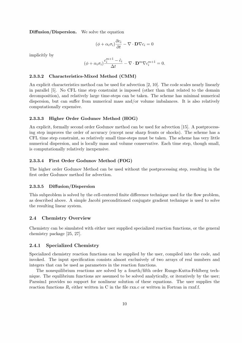
Diffusion/Dispersion. We solve the equation
(φ+ αiσi)∂ci∂t
−∇ ·D∇ci = 0
implicitly by
(φ+ αiσi)cm+1i − ci
∆t−∇ ·Dm∇cm+1
i = 0.
2.3.3.2 Characteristics-Mixed Method (CMM)
An explicit characteristics method can be used for advection [2, 10]. The code scales nearly linearlyin parallel [5]. No CFL time step constraint is imposed (other than that related to the domaindecomposition), and relatively large time-steps can be taken. The scheme has minimal numericaldispersion, but can suffer from numerical mass and/or volume imbalances. It is also relativelycomputationally expensive.
2.3.3.3 Higher Order Godunov Method (HOG)
An explicit, formally second order Godunov method can be used for advection [15]. A postprocess-ing step improves the order of accuracy (except near sharp fronts or shocks). The scheme has aCFL time step constraint, so relatively small time-steps must be taken. The scheme has very littlenumerical dispersion, and is locally mass and volume conservative. Each time step, though small,is computationally relatively inexpensive.
2.3.3.4 First Order Godunov Method (FOG)
The higher order Godunov Method can be used without the postprocessing step, resulting in thefirst order Godunov method for advection.
2.3.3.5 Diffusion/Dispersion
This subproblem is solved by the cell-centered finite difference technique used for the flow problem,as described above. A simple Jacobi preconditioned conjugate gradient technique is used to solvethe resulting linear system.
2.4 Chemistry Overview
Chemistry can be simulated with either user supplied specialized reaction functions, or the generalchemistry package [25, 27].
2.4.1 Specialized Chemistry
Specialized chemistry reaction functions can be supplied by the user, compiled into the code, andinvoked. The input specification consists almost exclusively of two arrays of real numbers andintegers that can be used as parameters in the reaction functions.
The nonequilibrium reactions are solved by a fourth/fifth order Runge-Kutta-Fehlberg tech-nique. The equilibrium functions are assumed to be solved analytically, or iteratively by the user;Parssim1 provides no support for nonlinear solution of these equations. The user supplies thereaction functions Ri either written in C in the file rxn.c or written in Fortran in rxnf.f.
10
2.4.2 General Chemistry Package
Reactive transport in porous media can be simulated with a full complement of homogeneous andheterogeneous reactions (complexation, adsorption, ion-exchange and precipitation/dissolution) ofboth equilibrium and kinetic type. Kinetics are assumed to be of the mass-action “distance-from-equilibrium” type, where the reaction rate is proportional to the product of powers of componentconcentrations.
The package also permits generalised Monod-style rate expressions. This means that manybiochemical, biodegradation and bioremediation reactions can be incorporated directly into thegeneral chemistry computation.
The chemistry reactions should be set up as if they were in a batch system; that is, the reactionrates should be given on a moles per unit pore volume (i.e., flowing phase volume) basis. Reactionsare not computed in the wells.
Three options exist for the choice of equilibrium module, namely SF (stoichiometric formula-tion), UNSF (unreduced non-stoichiometric formulation) and RNSF (reduced non-stoichiometricformulation). These options are described in detail in [25]. As a general guideline, we recommendthe RNSF version, as it is fastest for most problems that we have encountered. The SF version hasthe advantage of exact mass-balance and generalizes easier to multi-phase problems, but typicallyruns slower due to a larger number of variables (in particular, a larger number of Lagrange multi-pliers). The UNSF is prohibitively slow for realistic simulations and is included mainly for archivalreasons. The choice of version is made at the time of compilation.
2.4.3 Numerical Solution
An interior-point optimization technique [19, 26] is used to solve for the minimum of the Gibbs freeenergy.
2.5 General Chemistry
We reproduce here for convenience information from the chemistry manual [27]. Basic reactiontheory is presented. The variables in typewriter font refer to variables to be input as data asdescribed in the chapter on the input data file(s) (Chapter 5).
2.5.1 Thermodynamics
In this section we discuss the issues of phase-identity of a species, the usage of practical concen-tration scales versus computationally convenient ones and unit conversions. The versions that arebased on mole-fractions (i.e., SF and UNSF) differ from the molar concentration based version(RNSF), and we discuss these cases separately. In this section, we use notation established by Saafin his Ph.D. Thesis [25]. In particular, the system is comprised of NS species (nSpecies) of whichNC are components (nComps) and NR products (nProducts). When convenient, we distinguish NK
R
kinetic and NQR equilibrium products (NR = NK
R +NQR ). Finally, we let NM denote the number of
minerals and IM the corresponding index-set.
11
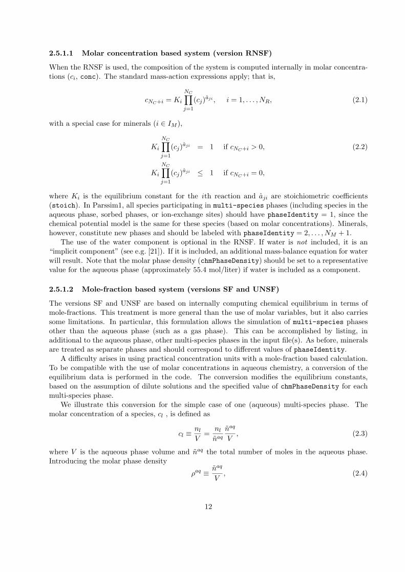
2.5.1.1 Molar concentration based system (version RNSF)
When the RNSF is used, the composition of the system is computed internally in molar concentra-tions (ci, conc). The standard mass-action expressions apply; that is,
cNC+i = Ki
NC∏j=1
(cj)aji , i = 1, . . . , NR, (2.1)
with a special case for minerals (i ∈ IM ),
Ki
NC∏j=1
(cj)aji = 1 if cNC+i > 0, (2.2)
Ki
NC∏j=1
(cj)aji ≤ 1 if cNC+i = 0,
where Ki is the equilibrium constant for the ith reaction and aji are stoichiometric coefficients(stoich). In Parssim1, all species participating in multi-species phases (including species in theaqueous phase, sorbed phases, or ion-exchange sites) should have phaseIdentity = 1, since thechemical potential model is the same for these species (based on molar concentrations). Minerals,however, constitute new phases and should be labeled with phaseIdentity = 2, . . . , NM + 1.
The use of the water component is optional in the RNSF. If water is not included, it is an“implicit component” (see e.g. [21]). If it is included, an additional mass-balance equation for waterwill result. Note that the molar phase density (chmPhaseDensity) should be set to a representativevalue for the aqueous phase (approximately 55.4 mol/liter) if water is included as a component.
2.5.1.2 Mole-fraction based system (versions SF and UNSF)
The versions SF and UNSF are based on internally computing chemical equilibrium in terms ofmole-fractions. This treatment is more general than the use of molar variables, but it also carriessome limitations. In particular, this formulation allows the simulation of multi-species phasesother than the aqueous phase (such as a gas phase). This can be accomplished by listing, inadditional to the aqueous phase, other multi-species phases in the input file(s). As before, mineralsare treated as separate phases and should correspond to different values of phaseIdentity.
A difficulty arises in using practical concentration units with a mole-fraction based calculation.To be compatible with the use of molar concentrations in aqueous chemistry, a conversion of theequilibrium data is performed in the code. The conversion modifies the equilibrium constants,based on the assumption of dilute solutions and the specified value of chmPhaseDensity for eachmulti-species phase.
We illustrate this conversion for the simple case of one (aqueous) multi-species phase. Themolar concentration of a species, cl , is defined as
cl ≡nl
V=
nl
naq
naq
V, (2.3)
where V is the aqueous phase volume and naq the total number of moles in the aqueous phase.Introducing the molar phase density
ρaq ≡ naq
V, (2.4)
12
and using the definition of the mole-fraction of the lth species, we can rewrite
cl = xlρaq. (2.5)
Substituting this in the original mass-action expression (2.1) yields
xNC+i = Kxi
NC∏j=1
(xj)aji , i = 1, . . . , NR, (2.6)
where the modified equilibrium constant Kxi satisfies
logKxi =
{logKi + (
∑NCj=1 aji) log ρaq if i is a mineral,
logKi + (∑NC
j=1 aji − 1) log ρaq otherwise(2.7)
Similar formulas can be derived if several multi-species phases are present.As stated above, the conversion assumes dilute solutions. If the actual molar phase density
changes drastically, the computed equilibrium will differ from that given by (2.1). Certainly for theaqueous phase the approximation is almost always an excellent one. Note that the solvent (water)must always be present in this formulation, and it is checked that the water component has beenspecified.
Finally note that, if desired, the user can specify chmPhaseDensity = 1.0 for a multi-speciesphase to perform the calculation in mole-fractions (consider e.g. (2.5)). Other units conversionswill need to be made carefully elsewhere in the input data file(s) (see §4.7.1 for the units conversioncapabilities of the code).
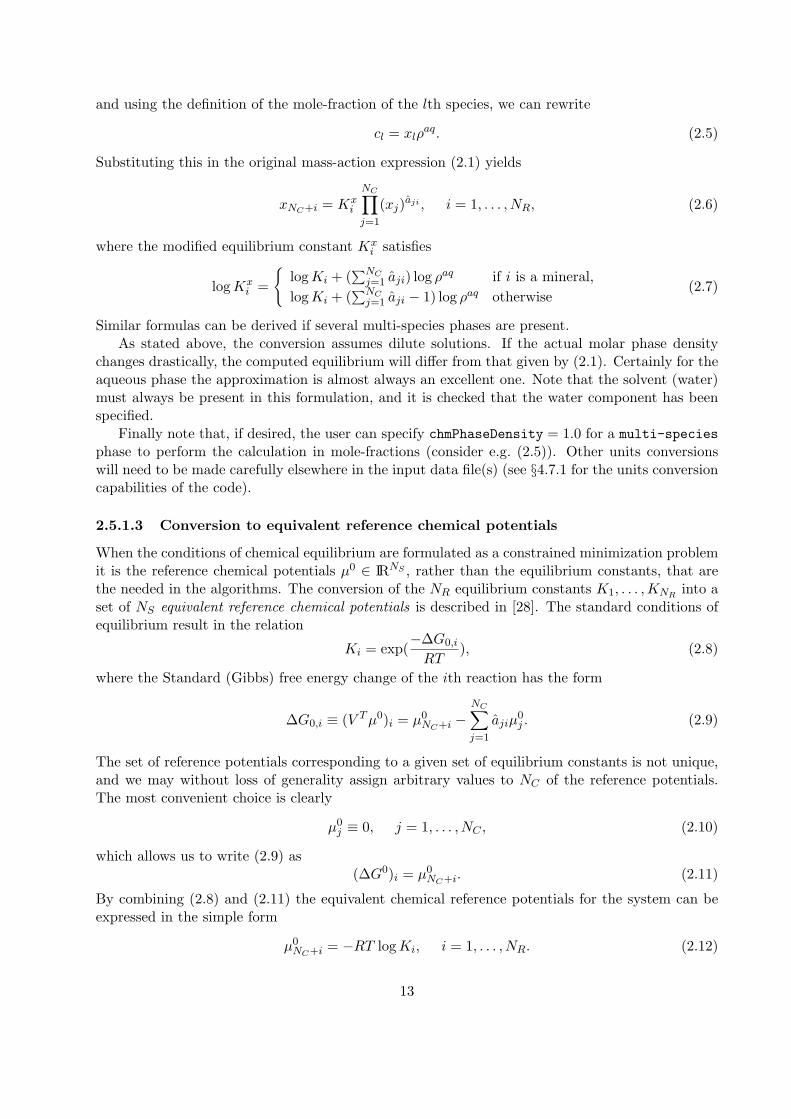
2.5.1.3 Conversion to equivalent reference chemical potentials
When the conditions of chemical equilibrium are formulated as a constrained minimization problemit is the reference chemical potentials µ0 ∈ IRNS , rather than the equilibrium constants, that arethe needed in the algorithms. The conversion of the NR equilibrium constants K1, . . . ,KNR
into aset of NS equivalent reference chemical potentials is described in [28]. The standard conditions ofequilibrium result in the relation
Ki = exp(−∆G0,i
RT), (2.8)
where the Standard (Gibbs) free energy change of the ith reaction has the form
∆G0,i ≡ (V Tµ0)i = µ0NC+i −
NC∑j=1
ajiµ0j . (2.9)
The set of reference potentials corresponding to a given set of equilibrium constants is not unique,and we may without loss of generality assign arbitrary values to NC of the reference potentials.The most convenient choice is clearly
µ0j ≡ 0, j = 1, . . . , NC , (2.10)
which allows us to write (2.9) as(∆G0)i = µ0
NC+i. (2.11)
By combining (2.8) and (2.11) the equivalent chemical reference potentials for the system can beexpressed in the simple form
µ0NC+i = −RT logKi, i = 1, . . . , NR. (2.12)
13

2.5.2 Kinetic reactions and their rate-laws
We allow fairly general rate-expressions for the NKR kinetic reactions. Expressions derived from
classical mass-action equilibrium are supported, as are generalized Monod type kinetic expressions.
2.5.2.1 Distance-from-equilibrium expressions
The distance from equilibrium has long been used as a measure of the driving force for change,in the present application for change in chemical composition. Specifically, we express the kineticrates rK
i as the difference between a forward and a backward rate
rKi = kf
i
NC∏j=1
(cj)pji − kbi cNC+i, i = 1, . . . , NK
R , (2.13)
where kfi and kb
i are the forward and backward rate constants, respectively, and p ∈ IRNC×NKR is a
matrix of powers on the components in the rate law. An important special case is the situation pij =aij , i.e., the powers on the component concentrations are equal to their stoichiometric coefficientsin the product species. This is the “classical” form of the rate-law. Note that with this choice, thereaction rate is zero if and only if the reaction satisfies the equilibrium conditions with an equivalentequilibrium constant of the form
Ki =kf
i
kbi
. (2.14)
This follows from the fact that
rKi = 0 ⇐⇒ kf
i
NC∏j=1
(cj)aji − kbi cNC+i = 0,
⇐⇒ kfi
kbi
NC∏j=1
(cj)aji − cNC+i = 0,
⇐⇒ cNC+i = Ki
NC∏j=1
(cj)aji .
The definition of the equilibrium constant for the completed reaction (2.14) allows species-switching(switchFlag) to be used (see also §2.5.3.3).
We point out that regardless of the choice of equilibrium module, the rate-laws always use molarconcentrations.
2.5.2.2 Monod style expressions
Monod introduced an empirical expression of the form
dX
dt= kX
S
K + S(2.15)
to account for the growth of microbes X on a substrate S. The constant K is commonly referredto as the “half saturation constant” (halfSatConst). This expression is widely used to modelbiologically mediated reactions. We allow a generalized version of this expression:
rKi = kf
i
NC∏j=1
(cj)pji
NC∏j=1
cj
Khalfij + cj
− kbi cNC+i, i = 1, . . . , NM
R , (2.16)
14
where Khalfij are the half saturation constants for the component species (more than one component
is allowed to participate in each reaction) and NMR is the number of Monod style rate expressions.
Any or all or none of the NKR kinetic reactions may have Monod-style expressions, i.e., 0 ≤ NM
R ≤NK
R . When Khalfij = 0 for all j the Monod expression reduces to the distance-from-equilibrium
expression. Typical bioreactions are irreversible, and the backward rate constant kbi is usually set
to zero.
2.5.2.3 Kinetic reaction products
It may happen that several kinetic reactions yield a common product or by-product, e.g., carbondioxide, or that a single reaction produces multiple products. The framework described abovemakes no explicit accommodation of these possibilities, but it can in fact be extended to thesesituations. The trick is to define some common products or by-products as components and assignthem negative stoichiometric coefficients (stoichK) in the reactions for the other product species.
2.5.3 Numerical parameters
We now discuss appropriate settings for the chemistry solution parameters (in §5.2.3). For some ofthese parameters, useful default values are given there.
The parameter chmLoadBalFlag specifies whether automatic parallel load balancing of thecomputational work among processors should be attempted. This creates parallel communicationoverhead, but generally speeds up the computation in parallel.
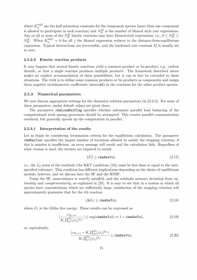
2.5.3.1 Interpretation of the results
Let us begin by considering termination criteria for the equilibrium calculation. The parameterchmMaxIter specifies the largest number of iterations allowed to satisfy the stopping criterion; ifthis is number is insufficient, an error message will result and the calculation fails. Regardless ofwhat version is used, the iterates are required to satisfy
‖F‖ ≤ chmAbsTol, (2.17)
i.e., the L2 norm of the residuals (the KKT conditions [18]) must be less than or equal to the user-specified tolerance. This condition has different implications depending on the choice of equilibriummodule; however, and we discuss here the SF and the RNSF.
Using the SF, mass-balance is exactly satisfied, and the residuals measure deviation from op-timality and complementarity, as explained in [25]. It is easy to see that in a system in which allspecies have concentrations which are sufficiently large, satisfaction of the stopping criterion willapproximately guarantee that for the ith reaction
|∆Gi| ≤ chmAbsTol, (2.18)
where Gi is the Gibbs free energy. These results can be expressed as
| cNC+i
Ki∏NC
j=1(cj)aji| ≤ exp(chmAbsTol) ≈ 1 + chmAbsTol, (2.19)
or, equivalently,|cNC+i −Ki
∏NCj=1(cj)
aji |Ki
∏NCj=1(cj)
aji≤ chmAbsTol, (2.20)
15
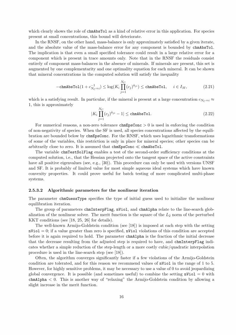
which clearly shows the role of chmAbsTol as a kind of relative error in this application. For speciespresent at small concentrations, this bound will deteriorate.
In the RNSF, on the other hand, mass-balance is only approximately satisfied by a given iterate,and the absolute value of the mass-balance error for any component is bounded by chmAbsTol.The implication is that even a small specified tolerance could result in a large relative error for acomponent which is present in trace amounts only. Note that in the RNSF the residuals consistentirely of component mass-balances in the absence of minerals. If minerals are present, this set isaugmented by one complementarity and one optimality equation for each mineral. It can be shownthat mineral concentrations in the computed solution will satisfy the inequality
−chmAbsTol(1 + c−1NC+i) ≤ log(Ki
NC∏j=1
(cj)aji) ≤ chmAbsTol, i ∈ IM , (2.21)
which is a satisfying result. In particular, if the mineral is present at a large concentration cNC+i ≈1, this is approximately
|Ki
NC∏j=1
(cj)aji − 1| ≤ chmAbsTol. (2.22)
For numerical reasons, a non-zero tolerance chmEpsConc > 0 is used in enforcing the conditionof non-negativity of species. When the SF is used, all species concentrations affected by the equili-bration are bounded below by chmEpsConc. For the RNSF, which uses logarithmic transformationsof some of the variables, this restriction is only in place for mineral species; other species can bearbitrarily close to zero. It is assumed that chmEpsConc� chmAbsTol.
The variable chmTestSolFlag enables a test of the second-order sufficiency conditions at thecomputed solution, i.e., that the Hessian projected onto the tangent space of the active constraintshave all positive eigenvalues (see, e.g., [30]). This procedure can only be used with versions UNSFand SF. It is probably of limited value for most simple aqueous ideal systems which have knownconvexity properties. It could prove useful for batch testing of more complicated multi-phasesystems.
2.5.3.2 Algorithmic parameters for the nonlinear iteration
The parameter chmGuessType specifies the type of initial guess used to initialize the nonlinearequilibration iteration.
The group of parameters chmInterpFlag, nViol, and chmAlpha relate to the line-search glob-alization of the nonlinear solver. The merit function is the square of the L2 norm of the perturbedKKT conditions (see [18, 25, 26] for details).
The well-known Armijo-Goldstein condition (see [18]) is imposed at each step with the settingnViol = 0; if a value greater than zero is specified, nViol violations of this condition are acceptedbefore it is again required to hold. The parameter chmAlpha is the fraction of the initial decreasethat the decrease resulting from the adjusted step is required to have, and chmInterpFlag indi-cates whether a simple reduction of the step-length or a more costly cubic/quadratic interpolationprocedure is used in the line-search step (see [18]).
Often, the algorithm converges significantly faster if a few violations of the Armijo-Goldsteincondition are tolerated, and for this reason we recommend values of nViol in the range of 1 to 5.However, for highly sensitive problems, it may be necessary to use a value of 0 to avoid jeopardizingglobal convergence. It is possible (and sometimes useful) to combine the setting nViol = 0 withchmAlpha < 0. This is another way of “relaxing” the Armijo-Goldstein condition by allowing aslight increase in the merit function.
16
The variables tauMin and chmRho are directly related to the interior-point algorithms. VariabletauMin describes the smallest percentage of the movement to the non-negativity boundary that isallowed. It should be taken close to (but strictly less than) unity.
The parameter chmRho is the fraction by which the perturbation parameter in the interior-pointmethod (see [26]) is decreased as the solution is approached. It is always less than unity. Typically,a small value gives the fastest convergence, but too small a value may lead to the global convergenceproblem of “sticking to the boundary” (see [19]).
Note that the settings of tauMin and chmRho are of importance only when inequality constraintsare present in the formulation. Thus, if the RNSF version is used to solve a problem without mineralphases, these settings are of no consequence.
2.5.3.3 ODE integration control
The parameters ntReact, odeAlgType and switchFlag control the time-integration of the ODEsgoverning kinetic reactions and are only used if such reactions are specified by reactionType.
The variable odeAlgType controls the type of explicit time-stepping scheme used for the inte-gration. Currently, the choices 0, 1, 2 are supported, corresponding to the use of Forward-Euler(FE) first-order scheme, second-order Runge-Kutta (RK-2) and fourth-order Runge-Kutta (RK-4).
The parameter ntReact defines a target time-step to be used in the kinetic integration. Itspecifies the smallest number of reaction steps per transport step that we consider adequate. Asan example, ntReact = 1 means that the integration of the ODEs will proceed with a time-stepequal to that used for transport. Internally to the chemistry routines, this time-step size will alwaysbe attempted at the beginning of a step; however, it may be cut during the step if non-negativityviolations are encountered.
We point out that the variable chmEpsConc plays the role of a user-specified approximate zeroconcentration in the kinetic integration. We do not allow any kinetic process to decrease a speciesconcentration below epsConc.
If switchFlag = 0, the sub-division into equilibrium and kinetic reactions will remain the samethroughout the simulation. This is the normal mode of operation. However, with the settingswitchFlag = 1, the algorithms will attempt to “switch” kinetic reactions that appear to havegone to completion to the equilibrium subset. The “equivalent” equilibrium constant defined in(2.14) is used for this purpose. We point out that if species-switching is used, all rate-laws shouldbe in the “classical” form, as noted above; otherwise, the results are unpredictable.
2.6 Radionuclide Decay
Radionuclide decay reactions can be handled by the chemistry routines or by a separate radionuclidedecay routine that is supplied. If used, it amounts to a time splitting of the radionuclide decayreactions. These exponential growth and decay reactions can be extremely stiff, and they are solvedby a diagonalization of the system to increase stability and robustness. The half-lives of the speciesmust be unique.
17
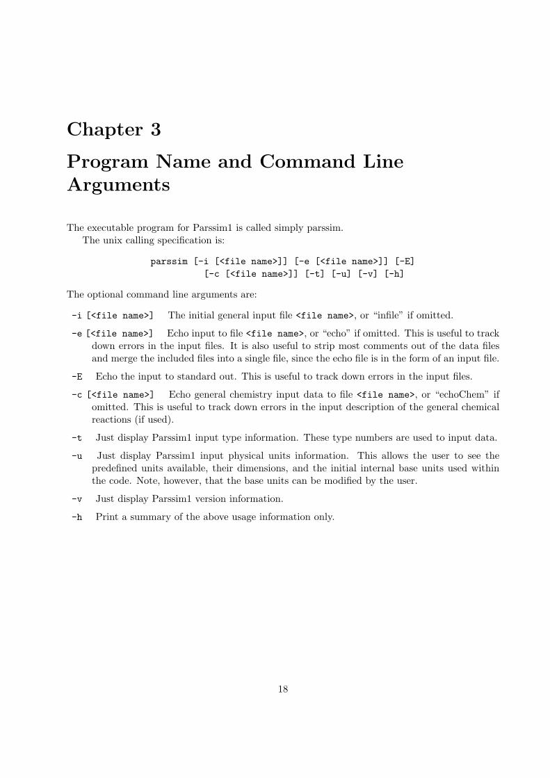
Chapter 3
Program Name and Command LineArguments
The executable program for Parssim1 is called simply parssim.The unix calling specification is:
parssim [-i [<file name>]] [-e [<file name>]] [-E][-c [<file name>]] [-t] [-u] [-v] [-h]
The optional command line arguments are:
-i [<file name>] The initial general input file <file name>, or “infile” if omitted.
-e [<file name>] Echo input to file <file name>, or “echo” if omitted. This is useful to trackdown errors in the input files. It is also useful to strip most comments out of the data filesand merge the included files into a single file, since the echo file is in the form of an input file.
-E Echo the input to standard out. This is useful to track down errors in the input files.
-c [<file name>] Echo general chemistry input data to file <file name>, or “echoChem” ifomitted. This is useful to track down errors in the input description of the general chemicalreactions (if used).
-t Just display Parssim1 input type information. These type numbers are used to input data.
-u Just display Parssim1 input physical units information. This allows the user to see thepredefined units available, their dimensions, and the initial internal base units used withinthe code. Note, however, that the base units can be modified by the user.
-v Just display Parssim1 version information.
-h Print a summary of the above usage information only.
18
Chapter 4
General Input File Syntax and Physical Units
All input is read from one or more data files. Key-words and data items are arranged in sections,subsections, and sub-subsections and ordered item-by-item, possibly separated by white-space,comments, and list delimiters, and possibly special commands.
4.1 White-space
White-space is used to separate other items, and is otherwise ignored on input. White-space consistsof the characters for space, tab, newline (or end-of-line), comma ‘,’, semicolon ‘;’, and colon ‘:’.White-space is ignored on input. The punctuation characters allow the user to delineate sets ofitems, for example.
Proper white-space consists of the characters for space, tab, and newline. Command names andkey-words are terminated by proper white-space.
4.2 Commands
Commands alter the way the data file(s) are read. Commands take the form command symbol ’$’followed immediately (no space) by a command name. Note that the command symbol is ignoredin any explicit comment and in skipped sectional units, but not before the first section (see thediscussion below on comments and sectinal units).
A list of commands follows.
$ Null command.
$$ Null command.
${# Equivalent to $BEGIN COMMENT.
$#} Equivalent to $END COMMENT.
$BEGIN COMMENT Causes input to be ignored until the matching $END COMMENT command is read(such commands are nested) or the end-of-file is reached.
$END COMMENT Terminates a $BEGIN COMMENT command.
$IGNORE LINES Follow by proper white-space and an integer. Causes that number of lines (i.e.,up to newline) to be ignored from the input stream. The line containing the integer is includedin the count of lines ignored, and information is ignored from that point on. However, theinclude command only is not ignored. This command can be used to ignore preambles inincluded data files.
19
$IGNORE WORDS Follow by proper white-space and an integer. Causes that number of words tobe ignored from the input stream. However, the include command only is not ignored. Thiscommand can be used to ignore preambles in included data files.
$INCLUDE Follow by proper white-space and a new file name (maximum of 50 characters). Thiscauses subsequent reading to take place in the new file. When the end-of-file is reached,reading commences in the original file. While there is no limit on the number of files thatmay be included, there is a maximum level to which they may be nested.
$LITERAL Terminates reading white-space and other symbols. This command is used to allow aspecial symbol at the beginning of a data string (such as punctuation ‘,’, ‘;’, and ‘:’, commentsymbol ‘#’, and command symbol ‘$’). (This command is not needed before $INCLUDE filenames.)
$S Equivalent to $SECTION.
$SECTION Begins a section of the data file. Follow by the section name.
$SS Equivalent to $SUBSECTION.
$SSS Equivalent to $SUBSUBSECTION.
$SUBSECTION Begins a subsection of the data file. Follow by the subsection name.
$SUBSUBSECTION Begins a sub-subsection of the data file. Follow by the sub-subsection name.
4.3 Comments
Explicit comments appear either after the comment symbol ‘#’ or between the $BEGIN COMMENT and$END COMMENT commands. A comment begun with ‘#’ runs to the newline symbol, so it can be usedto remove lines or ends of lines from a data file, without actually losing the information. (Note that‘#’ is an ordinary character if it is embedded in a string). It is acceptable to nest $BEGIN COMMENTand $END COMMENT commands.
Implicit comments can be made before the first section. Note that an unprocessed sectionalunit is an implicit comment. Moreover, sectional units given bogus names (such as “remark”) canbe used also as implicit comments.
4.4 Sectional Units
Sections, subsections, and sub-subsections are initiated by a $SECTION command, $SUBSECTIONcommand, or $SUBSUBSECTION command, respectively, and a specified string. It is important tonote that entire sectional units may be skipped on input if they are not needed according to theoptions specified by the data. This allows major routines to be omitted from the calculation (suchas flow, transport, or chemistry) without modifying the input file(s). If there is any doubt, one canuse the command line argument -e or -E to see if a given sectional unit was actually processed.
4.5 List Delimiters
List delimiters enclose lists that have a user specified number of items. A list is begun with a beginlist symbol ‘{’ and ended with an end list symbol ‘}’. The delimiters are used to check that theuser has counted the number of list items correctly.
20
4.6 Key-words
Key-words are specified strings of characters. Spaces may be embedded in a key-word.
4.7 Data Items
A data item can be an integer (not be followed by a period), a real number (in standard floatingpoint or exponential notation), a word of characters (terminated by a space, newline, or tab), or aline of characters (including spaces and tabs, terminated by a newline character).
Data items of characters are limited in length. The maximum allowed number of characters is:120 for a directory name;50 for a file name;120 for a line of character;30 for a word of characters;15 for phase and species names.
4.7.1 Physical Units
Real numbers have physical units. Physical units can be optionally assigned by using the squarebracket notation
<real> [<units expression>],
where the units expression may contain integer and real numbers, the names of units, arithmeticoperators, parentheses, and spaces (which are ignored). The statement declares the physical units ofthe number <real>, and causes the value to be converted into the set of base units used internally inthe code. The command line argument -e or -E displays the conversion computation for diagnosticpurposes. The base units can be set by the user (see §5.1 below).
A list of supported units, with their physical dimensions (and initial base unit numerical values),can be found by using the command line argument -u. The arithmetic operations supported areintegral exponentiation ‘**’ or ‘^’, multiplication ‘*’, division ‘/’, negation ‘-’, and parentheses ‘(’and ‘)’. Exponentiation by an integer with no physical dimensions only is allowed. We also allowaddition ‘+’ and subtraction ‘-’, though these should not appear in a units expression. The usualrules of precedence apply: exponentiation is performed first from left to right, then multiplicationand division, and finally addition and subtraction, although parentheses can be used to alter thisorder. A leading *’ or ‘/’ is allowed (a preceding ‘1’ is assumed).
Physical units are optional; the set of internal physical base units are assumed if none are given.If units are given, the physical dimensions must be proper for the given quantity or an error willresult. Dimension checking can be disabled by using double square bracket notation, as in
<number> [[<units expression>]],
in which case addition and subtraction are allowed. This also enables one to include the numericalvalues of unsupported units.
It is relatively easy for a programmer to add a new unit name to the code (or to change theinitial base units used internally in the code).
Temperature degree increments are an ordinary case of units as described above; however,temperature readings are a special case. These need simply the temperature scale used, degreesKelvin (degK), Celsius (degC), or Fahrenheit, (degF).
Examples follow.
21
2e-5 [cm/sec**2] # floating point notation is allowed8.2 [kg*m*sec^-2] # negation and integral exponentiation are allowed4.37 [[2]] # dimensions may be incorrect; value is doubled50 [/yr] # initial division is allowed1.2 [[2.1e-4 * (6 + 8.1^(cm/m)) / 2**3 + (cm/sec)^4]]
# nonsense, but a correctly formed expression100 [degC] # a temperature reading
4.7.2 Data Blocks and the Repetition Symbol
Data items may come in a block of data, as when a grid array (see below) is specified. Such adata block is bounded by the list delimiter symbols ‘{’ and ‘}’, as described above. Within such ablock, the repetition character ‘@’ may be used. A set of “n” single data items, each with the value“value,” may be indicated by
n@value.
Proper white-space may precede “value,” but only spaces may precede ‘@’.Units may be specified for the real numbers in a data block, but only for the list as a whole;
that is, only a single expression can be given, and it applies to each number of the data block. Theunits expression must appear just before the list of numbers, as in
{ [cm^3/sec] 2.1 3.2 [email protected] ... }.
4.7.3 Grid Arrays: Constant, Nearly Constant, and Fully Specified
Data may be distributed in space and therefore assigned to every cell or point of the grid in 3-D,or in 2-D to every face or point of the domain boundary. The data per grid cell may be a singlenumerical value or a set of numerical values of a given fixed size. A uniform syntax is used tospecify such an array.
Within the array, the x coordinate varies most rapidly, then y, and finally z (as in Fortran). Forcell-centered data, the index range goes from 1 to the number of grid cells in the given direction(i.e., the full range is (1:nx,1:ny,1:nz)). For point-centered data, the index range goes from 0to the number of grid cells in the given direction (i.e., the full range is (0:nx,0:ny,0:nz)). Forface-centered data, the index range depends on the type of face considered. For an x-face, the arrayis point-centered in the x-direction and cell-centered in the other directions; similarly for a y-faceand a z-face (i.e., the full range is (0:nx,1:ny,1:nz), (1:nx,0:ny,1:nz), and (1:nx,1:ny,0:nz)for x-face, y-face, and z-face face-centered data, respectively.)
A grid array that consists of a single set of repeated values (i.e., a constant set of values) canbe specified as
constant <value(s)>,
where, if the values are real numbers, each may have units. The number of values needed is thenumber that the array requires per grid cell or point.
A grid array that consists of a few repeated sets of values (i.e., an array that is nearly constant)can be specified easily. For a 3-D array of grid cell or point values, the specification is
nearly constant <primary value(s)><number not that or those values>{
22
<low x index> : <high x index> , <low y index> : <high y index> ,<low z index> : <high z index> ; <value(s)>
...},
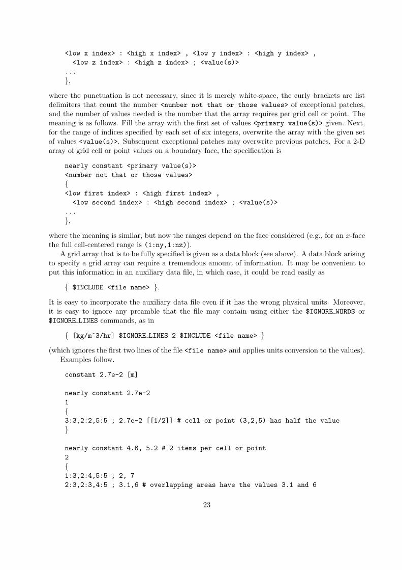
where the punctuation is not necessary, since it is merely white-space, the curly brackets are listdelimiters that count the number <number not that or those values> of exceptional patches,and the number of values needed is the number that the array requires per grid cell or point. Themeaning is as follows. Fill the array with the first set of values <primary value(s)> given. Next,for the range of indices specified by each set of six integers, overwrite the array with the given setof values <value(s)>. Subsequent exceptional patches may overwrite previous patches. For a 2-Darray of grid cell or point values on a boundary face, the specification is
nearly constant <primary value(s)><number not that or those values>{<low first index> : <high first index> ,<low second index> : <high second index> ; <value(s)>
...},
where the meaning is similar, but now the ranges depend on the face considered (e.g., for an x-facethe full cell-centered range is (1:ny,1:nz)).
A grid array that is to be fully specified is given as a data block (see above). A data block arisingto specify a grid array can require a tremendous amount of information. It may be convenient toput this information in an auxiliary data file, in which case, it could be read easily as
{ $INCLUDE <file name> }.
It is easy to incorporate the auxiliary data file even if it has the wrong physical units. Moreover,it is easy to ignore any preamble that the file may contain using either the $IGNORE WORDS or$IGNORE LINES commands, as in
{ [kg/m^3/hr] $IGNORE LINES 2 $INCLUDE <file name> }
(which ignores the first two lines of the file <file name> and applies units conversion to the values).Examples follow.
constant 2.7e-2 [m]
nearly constant 2.7e-21{3:3,2:2,5:5 ; 2.7e-2 [[1/2]] # cell or point (3,2,5) has half the value}
nearly constant 4.6, 5.2 # 2 items per cell or point2{1:3,2:4,5:5 ; 2, 72:3,2:3,4:5 ; 3.1,6 # overlapping areas have the values 3.1 and 6
23
}
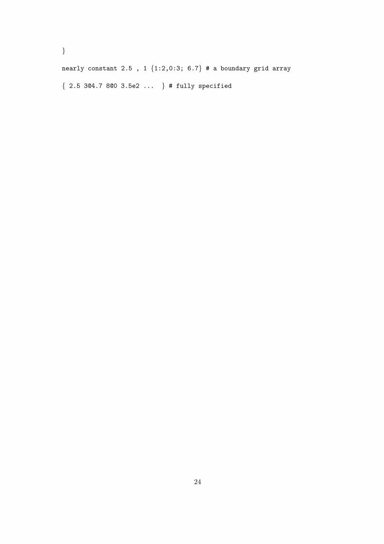
nearly constant 2.5 , 1 {1:2,0:3; 6.7} # a boundary grid array
{ 2.5 [email protected] 8@0 3.5e2 ... } # fully specified
24
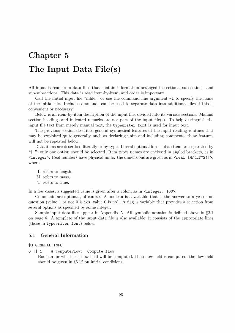
Chapter 5
The Input Data File(s)
All input is read from data files that contain information arranged in sections, subsections, andsub-subsections. This data is read item-by-item, and order is important.
Call the initial input file “infile,” or use the command line argument -i to specify the nameof the initial file. Include commands can be used to separate data into additional files if this isconvenient or necessary.
Below is an item-by-item description of the input file, divided into its various sections. Manualsection headings and indented remarks are not part of the input file(s). To help distinguish theinput file text from merely manual text, the typewriter font is used for input text.
The previous section describes general syntactical features of the input reading routines thatmay be exploited quite generally, such as declaring units and including comments; these featureswill not be repeated below.
Data items are described literally or by type. Literal optional forms of an item are separated by“||”; only one option should be selected. Item types names are enclosed in angled brackets, as in<integer>. Real numbers have physical units: the dimensions are given as in <real [M/(LT^2)]>,where
L refers to length,M refers to mass,T refers to time.
In a few cases, a suggested value is given after a colon, as in <integer: 100>.Comments are optional, of course. A boolean is a variable that is the answer to a yes or no
question (value 1 or not 0 is yes, value 0 is no). A flag is variable that provides a selection fromseveral options as specified by some integer.
Sample input data files appear in Appendix A. All symbolic notation is defined above in §2.1on page 6. A template of the input data file is also available; it consists of the appropriate lines(those in typewriter font) below.
5.1 General Information
$S GENERAL INFO
0 || 1 # computeFlow: Compute flowBoolean for whether a flow field will be computed. If no flow field is computed, the flow fieldshould be given in §5.12 on initial conditions.
25
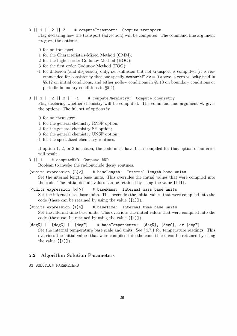
0 || 1 || 2 || 3 # computeTransport: Compute transportFlag declaring how the transport (advection) will be computed. The command line argument-t gives the options:
0 for no transport;1 for the Characteristics-Mixed Method (CMM);2 for the higher order Godunov Method (HOG);3 for the first order Godunov Method (FOG);
-1 for diffusion (and dispersion) only, i.e., diffusion but not transport is computed (it is rec-ommended for consistency that one specify computeFlow = 0 above, a zero velocity field in§5.12 on initial conditions, and either noflow conditions in §5.13 on boundary conditions orperiodic boundary conditions in §5.4).
0 || 1 || 2 || 3 || -1 # computeChemistry: Compute chemistryFlag declaring whether chemistry will be computed. The command line argument -t givesthe options. The full set of options is:
0 for no chemistry;1 for the general chemistry RNSF option;2 for the general chemistry SF option;3 for the general chemistry UNSF option;
-1 for the specialized chemistry routines.
If option 1, 2, or 3 is chosen, the code must have been compiled for that option or an errorwill result.
0 || 1 # computeRND: Compute RNDBoolean to invoke the radionuclide decay routines.
[<units expression [L]>] # baseLength: Internal length base unitsSet the internal length base units. This overrides the initial values that were compiled intothe code. The initial default values can be retained by using the value [[1]].
[<units expression [M]>] # baseMass: Internal mass base unitsSet the internal mass base units. This overrides the initial values that were compiled into thecode (these can be retained by using the value [[1]]).
[<units expression [T]>] # baseTime: Internal time base unitsSet the internal time base units. This overrides the initial values that were compiled into thecode (these can be retained by using the value [[1]]).
[degK] || [degC] || [degF] # baseTemperature: [degK], [degC], or [degF]Set the internal temperature base scale and units. See §4.7.1 for temperature readings. Thisoverrides the initial values that were compiled into the code (these can be retained by usingthe value [[1]]).
5.2 Algorithm Solution Parameters
$S SOLUTION PARAMETERS
26
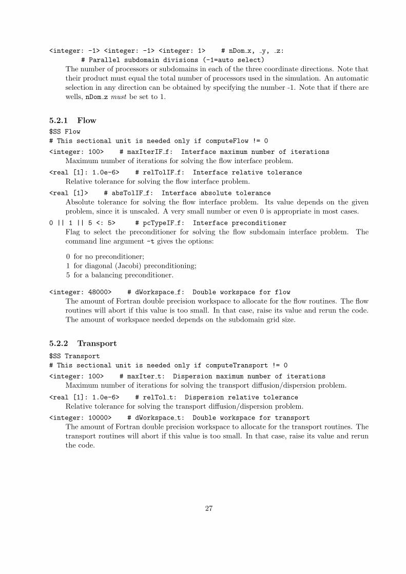
<integer: -1> <integer: -1> <integer: 1> # nDom x, y, z:# Parallel subdomain divisions (-1=auto select)
The number of processors or subdomains in each of the three coordinate directions. Note thattheir product must equal the total number of processors used in the simulation. An automaticselection in any direction can be obtained by specifying the number -1. Note that if there arewells, nDom z must be set to 1.
5.2.1 Flow
$SS Flow# This sectional unit is needed only if computeFlow != 0
<integer: 100> # maxIterIF f: Interface maximum number of iterationsMaximum number of iterations for solving the flow interface problem.
<real [1]: 1.0e-6> # relTolIF f: Interface relative toleranceRelative tolerance for solving the flow interface problem.
<real [1]> # absTolIF f: Interface absolute toleranceAbsolute tolerance for solving the flow interface problem. Its value depends on the givenproblem, since it is unscaled. A very small number or even 0 is appropriate in most cases.
0 || 1 || 5 <: 5> # pcTypeIF f: Interface preconditionerFlag to select the preconditioner for solving the flow subdomain interface problem. Thecommand line argument -t gives the options:
0 for no preconditioner;1 for diagonal (Jacobi) preconditioning;5 for a balancing preconditioner.
<integer: 48000> # dWorkspace f: Double workspace for flowThe amount of Fortran double precision workspace to allocate for the flow routines. The flowroutines will abort if this value is too small. In that case, raise its value and rerun the code.The amount of workspace needed depends on the subdomain grid size.
5.2.2 Transport
$SS Transport# This sectional unit is needed only if computeTransport != 0
<integer: 100> # maxIter t: Dispersion maximum number of iterationsMaximum number of iterations for solving the transport diffusion/dispersion problem.
<real [1]: 1.0e-6> # relTol t: Dispersion relative toleranceRelative tolerance for solving the transport diffusion/dispersion problem.
<integer: 10000> # dWorkspace t: Double workspace for transportThe amount of Fortran double precision workspace to allocate for the transport routines. Thetransport routines will abort if this value is too small. In that case, raise its value and rerunthe code.
27
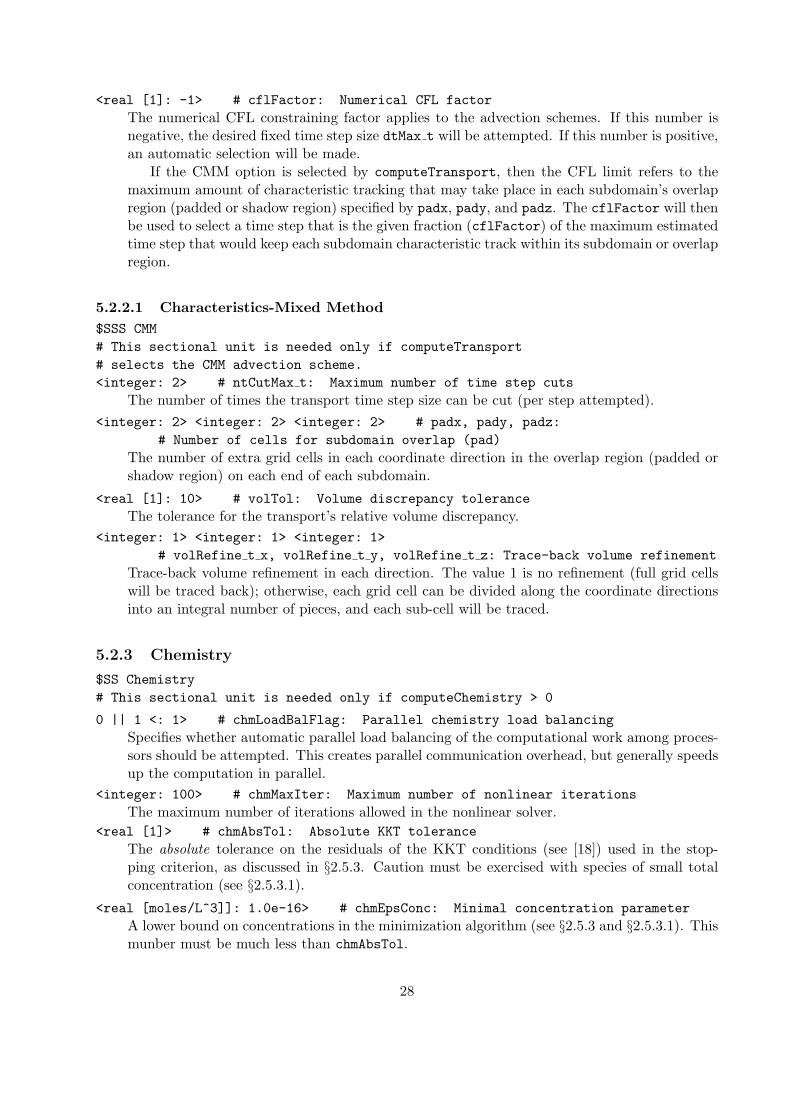
<real [1]: -1> # cflFactor: Numerical CFL factorThe numerical CFL constraining factor applies to the advection schemes. If this number isnegative, the desired fixed time step size dtMax t will be attempted. If this number is positive,an automatic selection will be made.
If the CMM option is selected by computeTransport, then the CFL limit refers to themaximum amount of characteristic tracking that may take place in each subdomain’s overlapregion (padded or shadow region) specified by padx, pady, and padz. The cflFactor will thenbe used to select a time step that is the given fraction (cflFactor) of the maximum estimatedtime step that would keep each subdomain characteristic track within its subdomain or overlapregion.
5.2.2.1 Characteristics-Mixed Method$SSS CMM# This sectional unit is needed only if computeTransport# selects the CMM advection scheme.<integer: 2> # ntCutMax t: Maximum number of time step cuts
The number of times the transport time step size can be cut (per step attempted).<integer: 2> <integer: 2> <integer: 2> # padx, pady, padz:
# Number of cells for subdomain overlap (pad)The number of extra grid cells in each coordinate direction in the overlap region (padded orshadow region) on each end of each subdomain.
<real [1]: 10> # volTol: Volume discrepancy toleranceThe tolerance for the transport’s relative volume discrepancy.
<integer: 1> <integer: 1> <integer: 1># volRefine t x, volRefine t y, volRefine t z: Trace-back volume refinement
Trace-back volume refinement in each direction. The value 1 is no refinement (full grid cellswill be traced back); otherwise, each grid cell can be divided along the coordinate directionsinto an integral number of pieces, and each sub-cell will be traced.
5.2.3 Chemistry
$SS Chemistry# This sectional unit is needed only if computeChemistry > 0
0 || 1 <: 1> # chmLoadBalFlag: Parallel chemistry load balancingSpecifies whether automatic parallel load balancing of the computational work among proces-sors should be attempted. This creates parallel communication overhead, but generally speedsup the computation in parallel.
<integer: 100> # chmMaxIter: Maximum number of nonlinear iterationsThe maximum number of iterations allowed in the nonlinear solver.
<real [1]> # chmAbsTol: Absolute KKT toleranceThe absolute tolerance on the residuals of the KKT conditions (see [18]) used in the stop-ping criterion, as discussed in §2.5.3. Caution must be exercised with species of small totalconcentration (see §2.5.3.1).
<real [moles/L^3]]: 1.0e-16> # chmEpsConc: Minimal concentration parameterA lower bound on concentrations in the minimization algorithm (see §2.5.3 and §2.5.3.1). Thismunber must be much less than chmAbsTol.
28
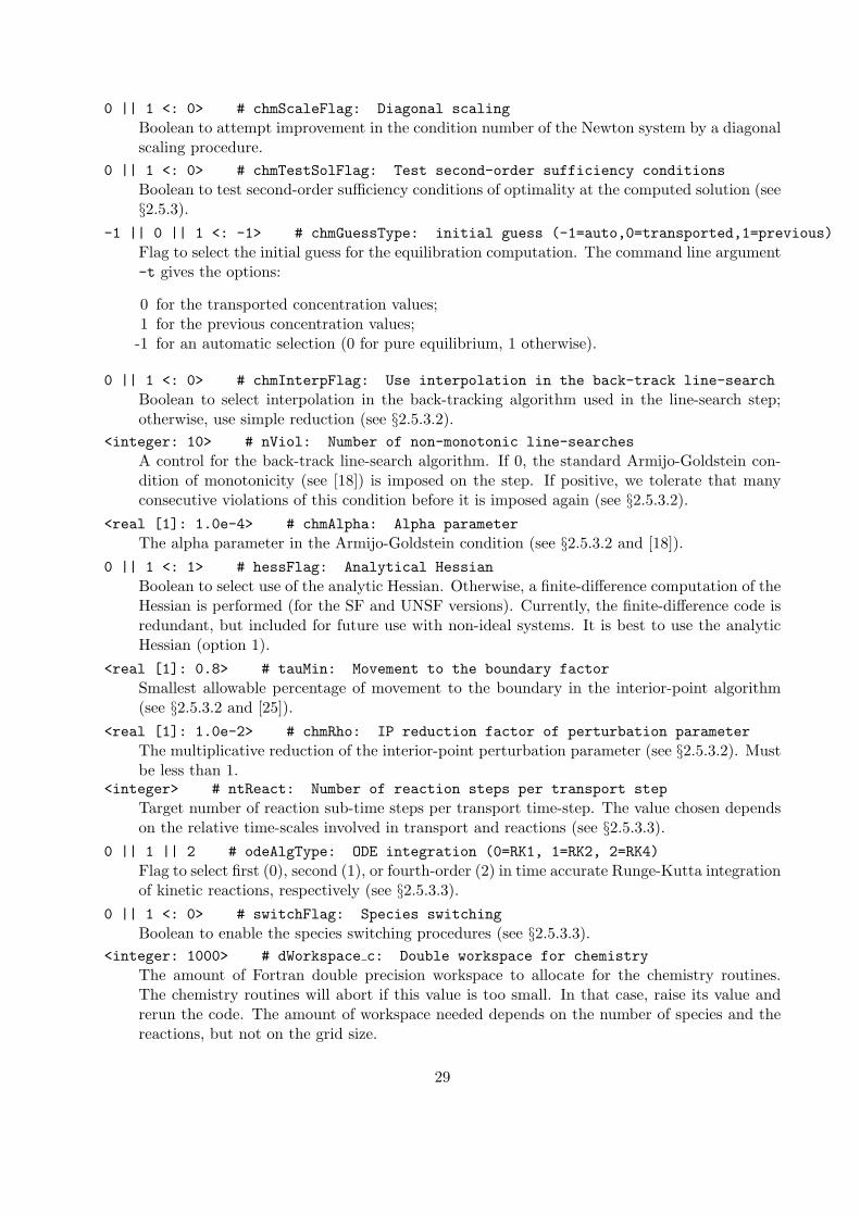
0 || 1 <: 0> # chmScaleFlag: Diagonal scalingBoolean to attempt improvement in the condition number of the Newton system by a diagonalscaling procedure.
0 || 1 <: 0> # chmTestSolFlag: Test second-order sufficiency conditionsBoolean to test second-order sufficiency conditions of optimality at the computed solution (see§2.5.3).
-1 || 0 || 1 <: -1> # chmGuessType: initial guess (-1=auto,0=transported,1=previous)Flag to select the initial guess for the equilibration computation. The command line argument-t gives the options:
0 for the transported concentration values;1 for the previous concentration values;
-1 for an automatic selection (0 for pure equilibrium, 1 otherwise).
0 || 1 <: 0> # chmInterpFlag: Use interpolation in the back-track line-searchBoolean to select interpolation in the back-tracking algorithm used in the line-search step;otherwise, use simple reduction (see §2.5.3.2).
<integer: 10> # nViol: Number of non-monotonic line-searchesA control for the back-track line-search algorithm. If 0, the standard Armijo-Goldstein con-dition of monotonicity (see [18]) is imposed on the step. If positive, we tolerate that manyconsecutive violations of this condition before it is imposed again (see §2.5.3.2).
<real [1]: 1.0e-4> # chmAlpha: Alpha parameterThe alpha parameter in the Armijo-Goldstein condition (see §2.5.3.2 and [18]).
0 || 1 <: 1> # hessFlag: Analytical HessianBoolean to select use of the analytic Hessian. Otherwise, a finite-difference computation of theHessian is performed (for the SF and UNSF versions). Currently, the finite-difference code isredundant, but included for future use with non-ideal systems. It is best to use the analyticHessian (option 1).
<real [1]: 0.8> # tauMin: Movement to the boundary factorSmallest allowable percentage of movement to the boundary in the interior-point algorithm(see §2.5.3.2 and [25]).
<real [1]: 1.0e-2> # chmRho: IP reduction factor of perturbation parameterThe multiplicative reduction of the interior-point perturbation parameter (see §2.5.3.2). Mustbe less than 1.
<integer> # ntReact: Number of reaction steps per transport stepTarget number of reaction sub-time steps per transport time-step. The value chosen dependson the relative time-scales involved in transport and reactions (see §2.5.3.3).
0 || 1 || 2 # odeAlgType: ODE integration (0=RK1, 1=RK2, 2=RK4)Flag to select first (0), second (1), or fourth-order (2) in time accurate Runge-Kutta integrationof kinetic reactions, respectively (see §2.5.3.3).
0 || 1 <: 0> # switchFlag: Species switchingBoolean to enable the species switching procedures (see §2.5.3.3).
<integer: 1000> # dWorkspace c: Double workspace for chemistryThe amount of Fortran double precision workspace to allocate for the chemistry routines.The chemistry routines will abort if this value is too small. In that case, raise its value andrerun the code. The amount of workspace needed depends on the number of species and thereactions, but not on the grid size.
29
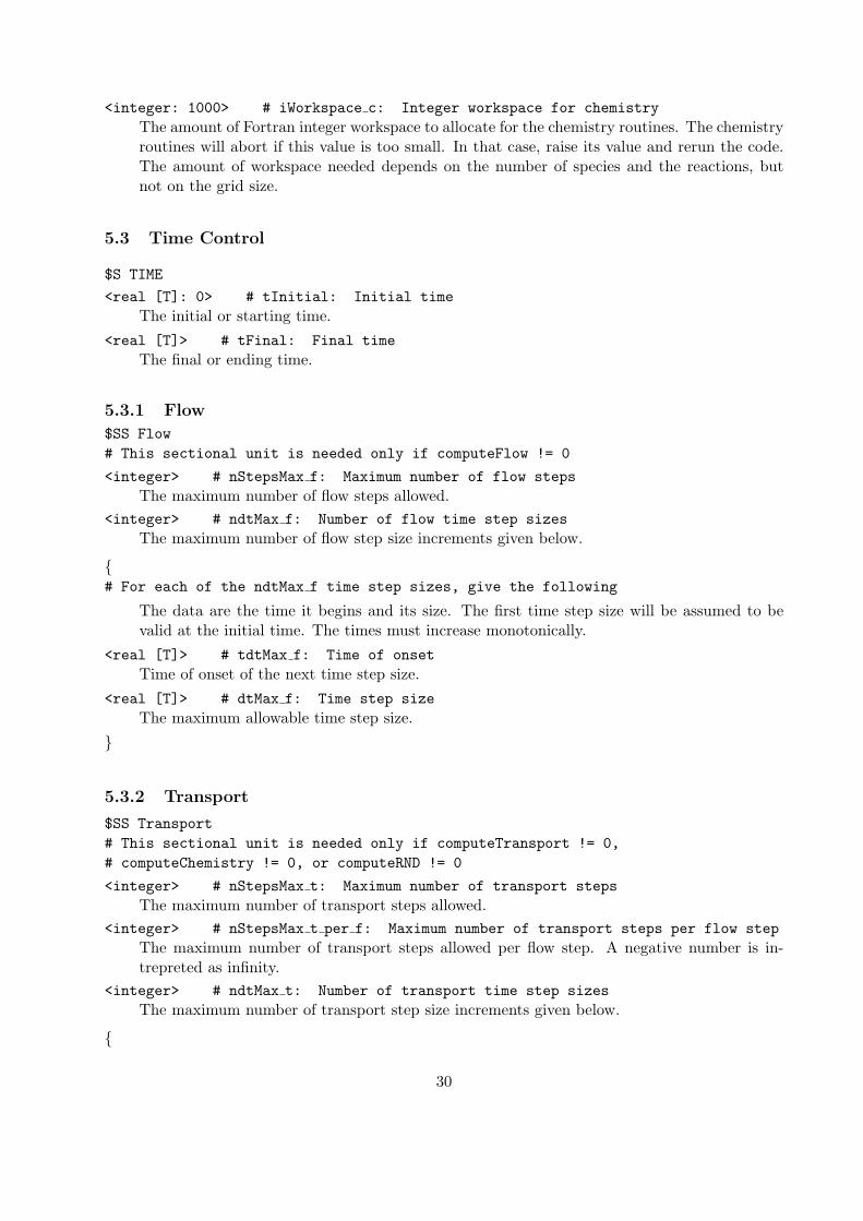
<integer: 1000> # iWorkspace c: Integer workspace for chemistryThe amount of Fortran integer workspace to allocate for the chemistry routines. The chemistryroutines will abort if this value is too small. In that case, raise its value and rerun the code.The amount of workspace needed depends on the number of species and the reactions, butnot on the grid size.
5.3 Time Control
$S TIME
<real [T]: 0> # tInitial: Initial timeThe initial or starting time.
<real [T]> # tFinal: Final timeThe final or ending time.
5.3.1 Flow
$SS Flow# This sectional unit is needed only if computeFlow != 0
<integer> # nStepsMax f: Maximum number of flow stepsThe maximum number of flow steps allowed.
<integer> # ndtMax f: Number of flow time step sizesThe maximum number of flow step size increments given below.
{# For each of the ndtMax f time step sizes, give the following
The data are the time it begins and its size. The first time step size will be assumed to bevalid at the initial time. The times must increase monotonically.
<real [T]> # tdtMax f: Time of onsetTime of onset of the next time step size.
<real [T]> # dtMax f: Time step sizeThe maximum allowable time step size.
}
5.3.2 Transport
$SS Transport# This sectional unit is needed only if computeTransport != 0,# computeChemistry != 0, or computeRND != 0
<integer> # nStepsMax t: Maximum number of transport stepsThe maximum number of transport steps allowed.
<integer> # nStepsMax t per f: Maximum number of transport steps per flow stepThe maximum number of transport steps allowed per flow step. A negative number is in-trepreted as infinity.
<integer> # ndtMax t: Number of transport time step sizesThe maximum number of transport step size increments given below.
{
30
# For each of the ndtMax t time step sizes, give the following
The data are the time it begins and its size. The first time step size will be assumed to bevalid at the initial time. The times must increase monotonically.
<real [T]> # tdtMax t: Time of onsetTime of onset of the next time step size.
<real [T]> # dtMax t: Time step sizeThe maximum allowable time step size.
}
5.4 Spatial Grid
$S GRID
<integer> <integer> <integer> # nx, ny, nz: Number of grid cellsThe number of grid cells (i.e., elements) in each coordinate direction.
<integer> <integer> <integer> # periodicBC x, y, z: Boolean for periodicitySet to 1 if the grid covers a periodic domain in the given coordinate direction (i.e., if there areperiodic boundary conditons).
0 || 1 # zIsDepth: Direction of the z coordinateBoolean for whether the z coordinate points down (depth) or up (height); that is, whether zincreases with depth or with height. We remark that internal to the code z points down.
uniform || rectangular || xy-rectangular || { # gridType:# uniform, rectangular, xy-rectangular, or {
The type of grid that is to be specified. The grid must be rectangular or logically rectangular.The options are:
• uniform for uniformly rectangular (i.e., each cell has the same dimensions);• rectangular for nonuniformly rectangular (i.e., each cell is rectangular, but they may vary
in size);• xy-rectangular for a grid that is nonuniform rectangular in x and y but fully variable in z;• { to specify a fully logically rectangular grid (this is the beginning of a data block).
This must be followed by one of the following sets of input data items.
5.4.1 Uniform Rectangular Grid
# Use the following when gridType is uniformgrid
<real [L]> <real [L]> # xMin, xMax: Minimal and maximal x pointsThe minimal and maximal x points of the computational grid.
<real [L]> <real [L]> # yMin, yMax: Minimal and maximal y pointsThe minimal and maximal y points of the computational grid.
<real [L]> <real [L]> # zMin, zMax: Minimal and maximal z pointsThe minimal and maximal z points of the computational grid.
31
5.4.2 Nonuniform Rectangular Grid
# Use the following when gridType is rectangular
{# For each of the nx+1 x grid points, give the following
<real [L]> # xp: The x grid points
}
{# For each of the ny+1 y grid points, give the following
<real [L]> # yp: The y grid points
}
{# For each of the nz+1 z grid points, give the following
<real [L]> # zp: The z grid points
}
5.4.3 An XY-rectangular, Z-variable Grid
# Use the following when gridType is xy-rectangular
{# For each of the nx+1 x grid points, give the following
<real [L]> # xp: The x grid points
}
{# For each of the ny+1 y grid points, give the following
<real [L]> # yp: The y grid points
}
{# For each of the (nx+1)*(ny+1)*(nz+1) z grid points, give the following
<real of a data block [L]> # zp: The z grid pointsSee §4.7.3 for information on a data block.
}
5.4.4 A Fully Logically Rectangular Grid
# Use the following when gridType is {This indicates the beginning of a data block
# For each of the (nx+1)*(ny+1)*(nz+1) x grid points, give:
<real of a data block [L]> # xp: The x grid pointsSee §4.7.3 for information on a data block.
32
}
{# For each of the (nx+1)*(ny+1)*(nz+1) y grid points, give the following
<real of a data block [L]> # yp: The y grid pointsSee §4.7.3 for information on a data block.
}
{# For each of the (nx+1)*(ny+1)*(nz+1) z grid points, give the following
<real of a data block [L]> # zp: The z grid pointsSee §4.7.3 for information on a data block.
}
5.5 Porous Medium Material Properties
$S MATERIAL PROPERTIES
<real [L/T^2]: 9.8 [m/sec^2]> # gravity: Gravitational constantThe gravitational constant.
<real grid array [1]> # porosity: PorosityA grid array of porosity values, given over the 3-D domain as cell-centered data, one per cell(see §4.7.3). An immobile phase can be accounted for by decreasing the porosity of the rockitself and entering those values here instead. Herein, pore volume refers to flowing phasevolume.
5.5.1 Permeabilities (or Conductivities)
$SS Permeability || $SS Conductivity# This sectional unit is needed only if computeFlow != 0
The meaning of the input “permeability” (perm) values is either the absolute permeability orthe hydraulic conductivity, depending on the subsection name. The hydraulic conductivityis K = ρgk/µ0. Permeability is assumed internal to the code. If an immobile fluid phaseis present, its effect on the flowing phase should be reflected in the values given below forthe permeability perm (i.e., give the product of the absolute permeability and the endpointrelative permeability, converted to conductivity if necessary).
scalar || diagonal || symmetric || face # permType:# scalar, diagonal, symmetric, or face
Declare the “permeability” to be a scalar (one value per cell), diagonal tensor (three valuesper cell), a full symmetric tensor (six values per cell), or face centered diagonal tensor values(a single value for each face of the grid). This must be followed by one of the following sets ofinput data items.
33

5.5.1.1 Scalar Permeabilities
# Use the following when permType is scalar
<real grid array [L^2 (permeability) or L/T (conductivity)]> # perm:# Scalar permeabilities
A grid array of scalar permeability values, given over the 3-D domain as cell-centered data,one per cell (see §4.7.3).
5.5.1.2 Diagonal Tensor Permeabilities
# Use the following when permType is diagonal
by cells || by components # permGrouping:# Group by grid cells or by tensor components
Give the entire permeability tensor for each grid cell, or give successively a single componentof the tensor for the entire grid. The word is optional.
xx yy zz || <any permutation> # permComponentOrder:# Order of tensor’s components
Declare the order of the permeability tensor component data.
<1 or 3 real grid arrays [L^2 (permeability) or L/T (conductivity)]> # perm:# Diagonal tensor permeabilities
One or three grid arrays of diagonal permeability values, given over the 3-D domain as cell-centered data, three or one number per cell (see §4.7.3). If the permGrouping is cells, give thethree components of the tensor (as ordered by permComponentOrder) for each grid cell. Oth-erwise, give three grid arrays of single item cell-centered data, one for each tensor component(again, as ordered by permComponentOrder).
5.5.1.3 Symmetric Tensor Permeabilities
# Use the following when permType is symmetric
cells || components # permGrouping:# Group by cells or by tensor components
Give the entire permeability tensor for each grid cell, or give successively a single componentof the tensor for the entire grid.
xx yy zz xy xz yz || <any permutation> # permComponentOrder:# Order of tensor’s components
Declare the order of the permeability tensor component data.
<1 or 6 real grid arrays [L^2 (permeability) or L/T (conductivity)]> # perm:# Symmetric tensor permeabilities
One or six grid arrays of symmetric tensor permeability values, given over the 3-D domainas cell-centered data, six or one number per cell (see §4.7.3). If the permGrouping is cells,give the six components of the tensor (as ordered by permComponentOrder) for each grid cell.Otherwise, give six grid arrays of single item cell-centered data, one for each tensor component(again, as ordered by permComponentOrder).
34
5.5.1.4 Face Permeabilities
# Use the following when permType is face
<3 real grid arrays [L^2 (permeability) or L/T (conductivity)]> # perm:# Face permeabilities
Three grid arrays of permeability values, given over the 3-D domain as face-centered data, oneper face (see §4.7.3). The arrays give values for the x-faces, y-faces, and z-faces and are ofsize (nx+1,ny,nz), (nx,ny+1,nz), and (nx,ny,nz+1)), respectively.
5.5.2 Dispersion
$SS Dispersion# This sectional unit is needed only if computeTransport != 0
The diffusion/dispersion tensor is defined above in §2.3.1 on page 8.<integer> # uniformDispersion: Flag for uniform dispersion
Flag for uniform dispersion if true (i.e., 1) or nonuniform if false (i.e., 0).
# Use this syntax if uniformDispersion is true (i.e., 1)
<real [L^2/T]> # molDiff: Molecular diffusionThe molecular diffusion coefficient.
<real [L]> # longDisp: Longitudinal dispersionThe longitudinal dispersion coefficient.
<real [L]> # transDisp: Transverse dispersionThe transverse dispersion coefficient.
# Use this syntax if uniformDispersion is false (i.e., 0)
<real grid array [L^2/T]> # molDiffAry: Molecular diffusion arrayThe molecular diffusion coefficient array.
<real grid array [L]> # longDispAry: Longitudinal dispersion arrayThe longitudinal dispersion coefficient array.
<real grid array [L]> # transDispAry: Transverse dispersion arrayThe transverse dispersion coefficient array.
5.5.3 Linear Sorption/Retardation
$SS Sorption# This sectional unit is needed only if computeTransport != 0,# computeChemistry != 0, or computeRND != 0
The linear sorption model is defined above in §2.3 and §2.3.2 (see pages 7 and 8).<integer> # nSorpTypes: Number of sorption types
The number of distinct sorption (or retardation) capacities.
{# For each of the nSorpTypes sorption types, give the following
This section induces an ordering of the sorption capacities that is used elsewhere.
35
<real grid array [1]> || porosity # sorp: Sorption capacitiesThe sorption capacities (σ). The option “porosity” implies that the retardation is propor-tional to porosity. Otherwise, give one value per cell (see §4.7.3).
}
5.6 Phase Properties
$S PHASE PROPERTIES
<real [M/(LT)]> # fluidViscosity: Flowing phase viscosityThe flowing phase viscosity of the resident fluid.
<real [M/L^3]> # fluidDensity: Flowing phase mass densityThe (average) flowing phase mass density. The fluid is assumed incompressible, so the densityof the fluid is not affected by its composition (i.e., we assume dilute solutions). This can causeinconsistencies if heavy or light components are present in the fluid in high concentrations.
<integer> # nPhases: Number of phasesThe total number of fluid and solid phases.
5.6.1 Phase Description
$SS Phase# Include one such sectional unit per phase as specified by nPhases
This section induces an ordering of the phases that is used elsewhere.<word of characters> # phaseNames: Phase name
The name of the phase. Maximum of 15 characters.
multi-species || single-species # phaseType: multi-species or single-speciesWhether the phase consists of multiple chemical species or a single chemical species. A multi-species phase is typically the flowing phase; single-species phases are typically minerals.
<real [1/L^3]> || <omit> # chmPhaseDensity: Molar densityThe molar density of the phase, in moles per fluid phase volume. This item occurs only ifphaseType is multi-species.
5.7 General Chemistry Properties
$S CHEMISTRY# This sectional unit is needed only if computeChemistry > 0
<real [temperature reading]> # absTemp: Equilibrium temperatureThe temperature at which equilibrium is computed. See §4.7.1 for temperature readings. Thisvalue is currently not used.
<real [M/(LT^2]> # chemPres: Equilibrium pressureA representative pressure at which equilibrium is computed. This value is currently not used.
ideal || non-ideal # ideal: ideal or non-idealIndicate whether all phases of the solution are to be considered ideal or non-ideal. Currently,only the ideal option is implemented.
36
5.8 Chemical Species Properties
$S CHEMICAL SPECIES
<integer> # nComps: Number of componentsThe number of chemical species that are components of the general chemistry reactions.
<integer> # nProducts: Number of productsThe number of chemical species that are products of the general chemistry reactions.
# nSpecies = nComps + nProductsFor ease of exposition and internal to the code, we let nSpecies be the sum of nComps andnProducts. If computeChemistry ≤ 0, so general chemistry is not used, nSpecies is the num-ber that is important, and it can be given by dividing arbitrarily the species into componentsand products above.
5.8.1 Species Description
$SS Component || $SS H Component || $SS H2O Component || $SS Product# Include one such sectional unit per component as specified by nComps# Follow by one such sectional unit per product as specified by nProducts
General chemistry requires knowledge of whether the species is a fundamental chemical com-ponent or a product of a reaction, and sometimes requires knowledge of where the hydrogenor water component is.
This sectional unit induces an ordering of the components, products, and species that isused elsewhere. Note that the species order places all components before all products; thatis, the component order index is the same as the species order index, and the product orderindex plus nComps is the species order index. Species are numbered beginning with 1.
<word of characters> # specieName: Specie nameThe name of the specie. Maximum of 15 characters.
<real [M]> # molecularWeight: Molecular weightThe molecular weight of the specie, in mass units per mole. This is used only for computingradionuclide decay and miscible displacement.
<real [1]> # phaseDist: The alpha parameter in Henry’s LawThe Henry’s Law constant for linear sorption. The linear sorption model is defined above in§2.3 and §2.3.2 (see pages 7 and 8). This is the parameter αi. A value of zero indicates thatno sorption takes place. A negative value indicates an immobile specie, and the value of αiσi
is assumed to be 1.<integer> || <omit> # sorpType: Sorption type
If needed (phaseDist > 0), the sorption capacity number from 1 to nSorpTypes specifiedearlier. This uses the order of the sorption capacities induced above.
$SSS Chemistry# This sectional unit is needed only if computeChemistry > 0
Components and products are described differently. The command line argument -c can beused to see how a given data set is interpreted.
37
5.8.1.1 Component Chemistry Specification
# Use this syntax if the subsection heading is Component,# H Component, or H2O Component
<integer> # phaseIdentity: Participating phaseThe phase in which the component participates, based on the organization of phases given inelsewhere.
<real [1]> # compCharge: ChargeThe intrinsic charge of the component. Used to compute the intrinsic species charges, and itcan be valuable for debugging the stoichiometry.
5.8.1.2 Product Chemistry Specification
# Use this syntax if the subsection heading is Product
<integer> # phaseIdentity: Participating phaseThe phase in which the product participates, based on the organization of phases given inelsewhere.
{# For each of the nComps components, give the following
<real [1]> # stoich: Stoichiometry formula numberThe formula number for this product species for the next component.
}0 || 1 || 2 # reactionType: Reaction type
Flag to select the class of reaction. The command line argument -t gives the options:
0 for equilibrium controlled;1 for mass-action type kinetic;2 for Monod type kinetic.
Equilibrium Reaction
# Use this syntax if reactionType specifies an equilibrium reaction
<real [1]> # pK: Log 10 equilibrium constantThe base 10 logarithm of the equilibrium constant.
Mass-action Type Kinetic Reaction
# Use this syntax if reactionType specifies a mass-action type kinetic reaction
<real [1]> <real [1]> # pKf, pKb: Log 10 forward and backward rate-constantsFor Kinetic reactions, give the base 10 logarithm of the forward and backward rate-constants.
{# For each of the nComps components, give the following
<real [1]> # stoichK: Rate-law powersPowers on the component-concentration in the rate-law. If taken equal to stoich, the “clas-sical” form of the rate-law results.
}
38
Monod Type Kinetic Reaction
# Use this syntax if reactionType specifies a monod type kinetic reaction
<real [1]> <real [1]: -99> # pKf, pKb: Log 10 forward & backward rate-constantsFor Kinetic reactions, give the base 10 logarithm of the forward and backward rate-constants.The backward rate-constant is included for generality; it is often not used in biochemicalpathways, and a small value (e.g., -99) should be assigned.
{# For each of the nComps components, give the following
<real [1]> # stoichK: Rate-law powersPowers on the component-concentration in the rate-law (2.16) (§2.5.2.2) in the form cpj . Com-ponents which appear in an expression of the form cj
K+cjare treated separately (see next set
of inputs) and should be given a power of 0 here.
}
{# For each of the nComps components, give the following
<real [1]> # halfSatConst: Half saturation constantsThe so-called “half-saturation constants” in Monod kinetics (2.16) (§2.5.2.2) which are theconstants K in terms of the form cj
K+cj. A component that does not appear in the rate
expression in this form should be given a value of 0 here.
}
5.9 Miscible Displacement
$S MISCIBLE DISPLACEMENT# This sectional unit is needed only if computeFlow != 0 and# computeTransport != 0, computeChemistry != 0, or computeRND != 0
0 || 1 # modelMiscDisp: Miscible displacement modelFlag declaring how the fluid viscosity will be computed in the flow computation. The commandline argument -t gives the options:
0 for a the fixed viscosity fluidViscosity;1 for the quarter power mixing rule.
5.9.1 Quarter Power Mixing Rule
# Use the following when modelMiscDisp selects# the quarter power mixing rulemodelMiscDisp
This rule is defined above in §2.2.1 on page 7.
{# For each of the nSpecies species, give the following
39
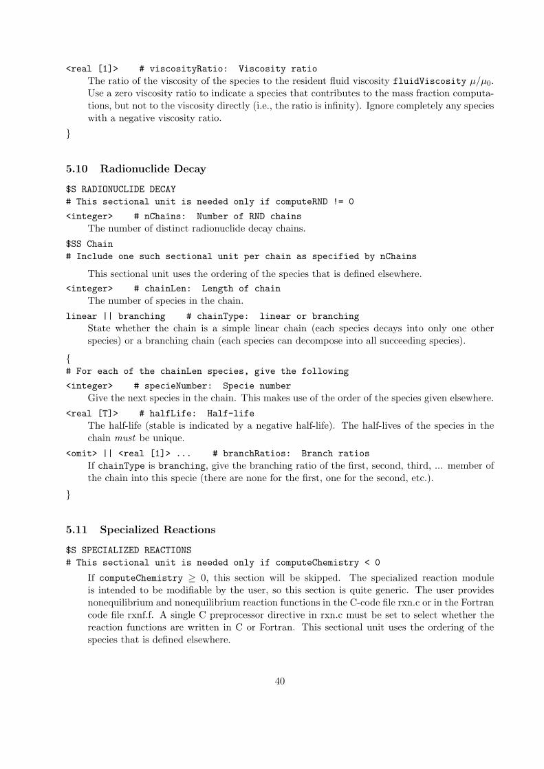
<real [1]> # viscosityRatio: Viscosity ratioThe ratio of the viscosity of the species to the resident fluid viscosity fluidViscosity µ/µ0.Use a zero viscosity ratio to indicate a species that contributes to the mass fraction computa-tions, but not to the viscosity directly (i.e., the ratio is infinity). Ignore completely any specieswith a negative viscosity ratio.
}
5.10 Radionuclide Decay
$S RADIONUCLIDE DECAY# This sectional unit is needed only if computeRND != 0
<integer> # nChains: Number of RND chainsThe number of distinct radionuclide decay chains.
$SS Chain# Include one such sectional unit per chain as specified by nChains
This sectional unit uses the ordering of the species that is defined elsewhere.<integer> # chainLen: Length of chain
The number of species in the chain.
linear || branching # chainType: linear or branchingState whether the chain is a simple linear chain (each species decays into only one otherspecies) or a branching chain (each species can decompose into all succeeding species).
{# For each of the chainLen species, give the following
<integer> # specieNumber: Specie numberGive the next species in the chain. This makes use of the order of the species given elsewhere.
<real [T]> # halfLife: Half-lifeThe half-life (stable is indicated by a negative half-life). The half-lives of the species in thechain must be unique.
<omit> || <real [1]> ... # branchRatios: Branch ratiosIf chainType is branching, give the branching ratio of the first, second, third, ... member ofthe chain into this specie (there are none for the first, one for the second, etc.).
}
5.11 Specialized Reactions
$S SPECIALIZED REACTIONS# This sectional unit is needed only if computeChemistry < 0
If computeChemistry ≥ 0, this section will be skipped. The specialized reaction moduleis intended to be modifiable by the user, so this section is quite generic. The user providesnonequilibrium and nonequilibrium reaction functions in the C-code file rxn.c or in the Fortrancode file rxnf.f. A single C preprocessor directive in rxn.c must be set to select whether thereaction functions are written in C or Fortran. This sectional unit uses the ordering of thespecies that is defined elsewhere.
40
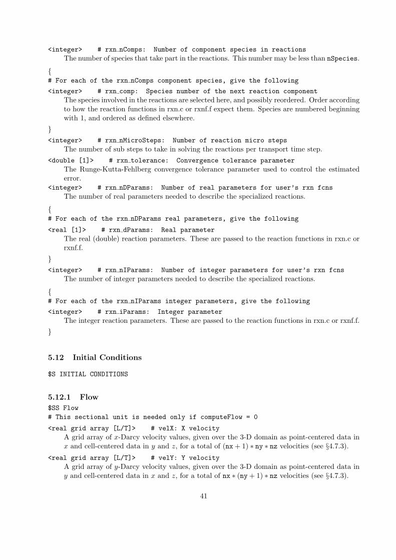
<integer> # rxn nComps: Number of component species in reactionsThe number of species that take part in the reactions. This number may be less than nSpecies.
{# For each of the rxn nComps component species, give the following
<integer> # rxn comp: Species number of the next reaction componentThe species involved in the reactions are selected here, and possibly reordered. Order accordingto how the reaction functions in rxn.c or rxnf.f expect them. Species are numbered beginningwith 1, and ordered as defined elsewhere.
}<integer> # rxn nMicroSteps: Number of reaction micro steps
The number of sub steps to take in solving the reactions per transport time step.
<double [1]> # rxn tolerance: Convergence tolerance parameterThe Runge-Kutta-Fehlberg convergence tolerance parameter used to control the estimatederror.
<integer> # rxn nDParams: Number of real parameters for user’s rxn fcnsThe number of real parameters needed to describe the specialized reactions.
{# For each of the rxn nDParams real parameters, give the following
<real [1]> # rxn dParams: Real parameterThe real (double) reaction parameters. These are passed to the reaction functions in rxn.c orrxnf.f.
}<integer> # rxn nIParams: Number of integer parameters for user’s rxn fcns
The number of integer parameters needed to describe the specialized reactions.
{# For each of the rxn nIParams integer parameters, give the following
<integer> # rxn iParams: Integer parameterThe integer reaction parameters. These are passed to the reaction functions in rxn.c or rxnf.f.
}
5.12 Initial Conditions
$S INITIAL CONDITIONS
5.12.1 Flow
$SS Flow# This sectional unit is needed only if computeFlow = 0
<real grid array [L/T]> # velX: X velocityA grid array of x-Darcy velocity values, given over the 3-D domain as point-centered data inx and cell-centered data in y and z, for a total of (nx + 1) ∗ ny ∗ nz velocities (see §4.7.3).
<real grid array [L/T]> # velY: Y velocityA grid array of y-Darcy velocity values, given over the 3-D domain as point-centered data iny and cell-centered data in x and z, for a total of nx ∗ (ny + 1) ∗ nz velocities (see §4.7.3).
41
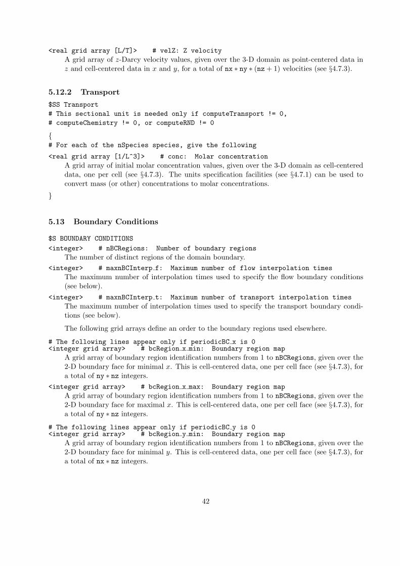
<real grid array [L/T]> # velZ: Z velocityA grid array of z-Darcy velocity values, given over the 3-D domain as point-centered data inz and cell-centered data in x and y, for a total of nx ∗ ny ∗ (nz + 1) velocities (see §4.7.3).
5.12.2 Transport
$SS Transport# This sectional unit is needed only if computeTransport != 0,# computeChemistry != 0, or computeRND != 0
{# For each of the nSpecies species, give the following
<real grid array [1/L^3]> # conc: Molar concentrationA grid array of initial molar concentration values, given over the 3-D domain as cell-centereddata, one per cell (see §4.7.3). The units specification facilities (see §4.7.1) can be used toconvert mass (or other) concentrations to molar concentrations.
}
5.13 Boundary Conditions
$S BOUNDARY CONDITIONS
<integer> # nBCRegions: Number of boundary regionsThe number of distinct regions of the domain boundary.
<integer> # maxnBCInterp f: Maximum number of flow interpolation timesThe maximum number of interpolation times used to specify the flow boundary conditions(see below).
<integer> # maxnBCInterp t: Maximum number of transport interpolation timesThe maximum number of interpolation times used to specify the transport boundary condi-tions (see below).
The following grid arrays define an order to the boundary regions used elsewhere.
# The following lines appear only if periodicBC x is 0<integer grid array> # bcRegion x min: Boundary region map
A grid array of boundary region identification numbers from 1 to nBCRegions, given over the2-D boundary face for minimal x. This is cell-centered data, one per cell face (see §4.7.3), fora total of ny ∗ nz integers.
<integer grid array> # bcRegion x max: Boundary region mapA grid array of boundary region identification numbers from 1 to nBCRegions, given over the2-D boundary face for maximal x. This is cell-centered data, one per cell face (see §4.7.3), fora total of ny ∗ nz integers.
# The following lines appear only if periodicBC y is 0<integer grid array> # bcRegion y min: Boundary region map
A grid array of boundary region identification numbers from 1 to nBCRegions, given over the2-D boundary face for minimal y. This is cell-centered data, one per cell face (see §4.7.3), fora total of nx ∗ nz integers.
42

<integer grid array> # bcRegion y max: Boundary region mapA grid array of boundary region identification numbers from 1 to nBCRegions, given over the2-D boundary face for maximal y. This is cell-centered data, one per cell face (see §4.7.3), fora total of nx ∗ nz integers.
# The following lines appear only if periodicBC z is 0<integer grid array> # bcRegion z min: Boundary region map
A grid array of boundary region identification numbers from 1 to nBCRegions, given over the2-D boundary face for minimal z. This is cell-centered data, one per cell face (see §4.7.3), fora total of nx ∗ ny integers.
<integer grid array> # bcRegion z max: Boundary region mapA grid array of boundary region identification numbers from 1 to nBCRegions, given over the2-D boundary face for maximal z. This is cell-centered data, one per cell face (see §4.7.3), fora total of nx ∗ ny integers.
5.13.1 Boundary Region Specification
$SS Region# Include one such sectional unit per boundary region as specified by nBCRegions
These regions are mapped to the physical boundary and ordered by the bcRegion grid arrays.
5.13.1.1 Flow$SSS Flow# This sectional unit is needed only if computeFlow != 0
0 || 1 || 2 # bcType f: BC typeFlag declaring the type of the boundary condition for flow. The command line argument -tgives the options:
0 for no flow condition, u · ν = 0 (0 normal velocity);1 for a Neumann condition −u · ν = qN (specified normal velocity, where the inflow condition
is positive and the outflow condition is negative);2 for a Dirichlet condition p = pN (specified pressure).
Above, qN or pN needs to be specified as a function of time.
Function of Time Specification
# The following lines appear only if a function of time# needs to be specified; that is, bcType f != 0
<omit> || pressure || potential || head || hydraulicHead # bcPresType in:# Dirichlet pressure, potential, head, or hydraulicHead
If bcType f selects the Dirichlet condition, give the meaning of the variable to which thecondition applies (see page 49 for a discussion on the meaning of the options).
<integer> # nBCInterp f: Number of interpolation timesThe number of interpolation times used in the definition of the boundary condition as apiecewise continuous linear function of time. Constant extrapolation is used before and afterthe first and last times; thus, a single interpolation time gives a constant condition. The timesmust not decrease; however, two pairs with the same time represent a discontinuous jump.
43
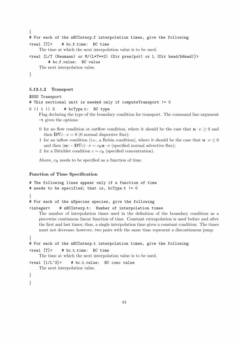
{# For each of the nBCInterp f interpolation times, give the following
<real [T]> # bc f time: BC timeThe time at which the next interpolation value is to be used.
<real [L/T (Neumann) or M/(L*T**2) (Dir pres/pot) or L (Dir head/hHead)]># bc f value: BC value
The next interpolation value.
}
5.13.1.2 Transport
$SSS Transport# This sectional unit is needed only if computeTransport != 0
0 || 1 || 2 # bcType t: BC typeFlag declaring the type of the boundary condition for transport. The command line argument-t gives the options:
0 for no flow condition or outflow condition, where it should be the case that u · ν ≥ 0 andthen D∇c · ν = 0 (0 normal dispersive flux);
1 for an inflow condition (i.e., a Robin condition), where it should be the case that u · ν ≤ 0and then (uc−D∇c) · ν = cBu · ν (specified normal advective flux);
2 for a Dirichlet condition c = cB (specified concentration).
Above, cB needs to be specified as a function of time.
Function of Time Specification
# The following lines appear only if a function of time# needs to be specified; that is, bcType t != 0
{# For each of the nSpecies species, give the following
<integer> # nBCInterp t: Number of interpolation timesThe number of interpolation times used in the definition of the boundary condition as apiecewise continuous linear function of time. Constant extrapolation is used before and afterthe first and last times; thus, a single interpolation time gives a constant condition. The timesmust not decrease; however, two pairs with the same time represent a discontinuous jump.
{# For each of the nBCInterp t interpolation times, give the following
<real [T]> # bc t time: BC timeThe time at which the next interpolation value is to be used.
<real [1/L^3]> # bc t value: BC conc valueThe next interpolation value.
}
}
44
5.14 Well Specification
$S WELLS
<integer> # nWells: Number of wellsThe number of wells. Note that if there are wells, nDom z must be set to 1 above.
<integer> # maxnWellInterp f: Maximum number of flow interpolation timesThe maximum number of interpolation times used to specify the flow well conditions (seebelow).
<integer> # maxnWellInterp t: Maximum number of transport interpolation timesThe maximum number of interpolation times used to specify the transport well conditions(see below).
5.14.1 Single Well Description
$SS Well# Include one such sectional unit per well as specified by nWells
0 || 1 || 2 || 3 || 4 # wellType: Well typeFlag specifying the type of the well. The command line argument -t gives the options:
0 for an inactive well;1 for an injection well;2 for an extraction well (or production well);3 for an bottomhole production well (that uses the Peaceman correction [23]);4 for an reinjection well (or sparging well).
A reinjection well has both an extraction and an injection interval; the fluid extracted isreinjected elsewhere. An inactive well is equivalent to no well at all, and no further specificationshould be given below.
# If the well is not inactive, include the following information
<real [L]> # wellRadius: Well radiusThe radius of the well.
<integer> <integer> # hWellIndex: The x and y indices of wellThe location of the well in the grid, given as the x and y cell-centered data index numbers.The well is generally assumed to occupy entire cells.
<integer> # zWellIndexLo: Lower z index of wellThe top (if zIsDepth is true) or bottom (otherwise) of the well in the grid, given as the lowerz cell-centered data index number. If wellType selects a reinjection well, specify the injectionpart.
<integer> # zWellIndexHi: Higher z index of wellThe bottom (if zIsDepth is true) or top (otherwise) of the well in the grid, given as the upperz cell-centered data index number. If wellType selects a reinjection well, specify the injectionpart.
<omit> || <integer> # zWellIndexLo: Lower z index of wellIf wellType selects a reinjection well, specify the lower z index number of the extraction part.
<omit> || <integer> # zWellIndexHi: Higher z index of wellIf wellType selects a reinjection well, specify the upper z index number of the extraction part.
45
5.14.1.1 Flow$SSS Flow# This sectional unit is needed only if computeFlow != 0
Bottomfole Producer
# Use if wellType selects a bottomhole producer
<real [M/(L*T^2)]> # wellPres: Well pressure potentialThe pressure potential of the well (see §2.1 on page 6 for the meaning of potential).
Other Active Well Types
# The following lines appear only if wellType does not select a bottomhole producer
<integer> # nWellInterp f: Number of interpolation timesThe number of interpolation times used in the definition of the wells as a piecewise continuouslinear function of time. Constant extrapolation is used before and after the first and last times;thus, a single interpolation time gives a constant condition. The times must not decrease;however, two pairs with the same time represent a discontinuous jump.
{# For each of the nWellInterp f interpolation times, give the following
<real [T]> # wellInj f time: Well timeThe time at which the next interpolation value is to be used.
<real [L^3/T]> # wellInj f value: Well injection or extraction rateThe next interpolation value, volume of injected or extracted fluid per unit time. It should benonnegative.
}
5.14.1.2 Transport
$SSS Transport# This sectional unit is needed only if computeTransport != 0 and# wellType does not select an extractor or a bottomhole producer
{# For each of the nSpecies species, give the following
<integer> # nWellInterp t: Number of interpolation timesThe number of interpolation times used in the definition of the boundary condition as apiecewise continuous linear function of time. Constant extrapolation is used before and afterthe first and last times; thus, a single interpolation time gives a constant condition. The timesmust not decrease; however, two pairs with the same time represent a discontinuous jump.
{# For each of the nWellInterp t interpolation times, give the following
<real [T]> # wellInj t time: Well timeThe time at which the next interpolation value is to be used.
46
<real [1/L^3]> # wellInj t value: Well conc valueThe next interpolation value, the molar concentration of the injected fluid.
}
}
5.15 Leaking Source Specification
$S LEAKS
<integer> # nLeaks: Number of leaksThe number of leaking sources.
<integer> # maxnLeakInterp: Maximum number of interpolation timesThe maximum number of interpolation times used to specify the leak conditions (see below).
5.15.1 Single Leak Description
$SS Leak# Include one such sectional unit per leak as specified by nLeaks
<integer> <integer> <integer> # leakIndexLo: Lower cell of leakThe leak occurs over a rectangular region. Specify the three indices of the lower cell of theleak in the grid, given as cell-centered data indices.
<integer> <integer> <integer> # leakIndexHi: Upper cell of leakThe leak occurs over a rectangular region. Specify the three indices of the upper cell of theleak in the grid, given as cell-centered data indices.
{# For each of the nSpecies species, give the following
<integer> # nLeakInterp: Number of interpolation timesThe number of interpolation times used in the definition of the leak as a piecewise continuouslinear function of time. Constant extrapolation is used before and after the first and last times;thus, a single interpolation time gives a constant condition. The times must not decrease;however, two pairs with the same time represent a discontinuous jump.
{# For each of the nLeakInterp interpolation times, give the following
<real [T]> # leakInj t time: Leak timeThe time at which the next interpolation value is to be used.
<real [1/T]> # leakInj t value: Leak conc valueThe next interpolation value, the molar rate of fluid leaking into the domain.
}
}
47
5.16 Output
$S OUTPUT
<integer> # runNumber: Run numberThe number of the current run. (Currently not used.)
<line of characters describing the run># runDescription: Title or description
A title or description of the current run. Maximum of 120 characters, including spaces.(Currently not used.)
0 || 1 # verbosity: Driver verbosity flagBoolean to monitor progress in the driver routines. A minimal amount of monitoring outputwill always be given.
0 || 1 || 2 || 3 || 4 # debug: Driver debug flagFlag to set the debug mode in the driver routines. The command line argument -t gives theoptions:
0 for no debugging tests or output;1 for debugging tests of the parallel set-up;2 for debugging output of miscellaneous items;3 for debugging output (dump) of the input data variables;4 for debugging output (dump) of the internal global variables.
The debugging level chosen includes everything at a lower level. Level 2 (and above) producesoutput. Output is written by each processor into its own file, called debug????, where theprocessor number replaces the question marks.
<word of characters> # outDir: Output directoryThe directory in which to write output data files. Use the $LITERAL command if the namebegins with a special symbol. The current directory is ‘.’ in unix. Maximum of 120 characters.
0 || 1 # outFormat3D: Output 3-D file formatFlag selecting the format for 3-D output data files. The command line argument -t gives theoptions:
-1 Eye visualization package format;0 raw data format;1 Tecplot visualization package format.
<integer> # nSpeciesPerOutfile: Number of species per 3-D output fileIf multiple species can appear in a single 3-D output file, this sets the maximum numberallowed.
0 || 1 # initialOut: Output 3-D initial conditions flagBoolean for giving output data files at the initial time.
1 # outFormat1D: Output 1-D file formatFlag selecting the format for 1-D output data files. The command line argument -t gives theoptions:
1 Tecplot visualization package format.
48
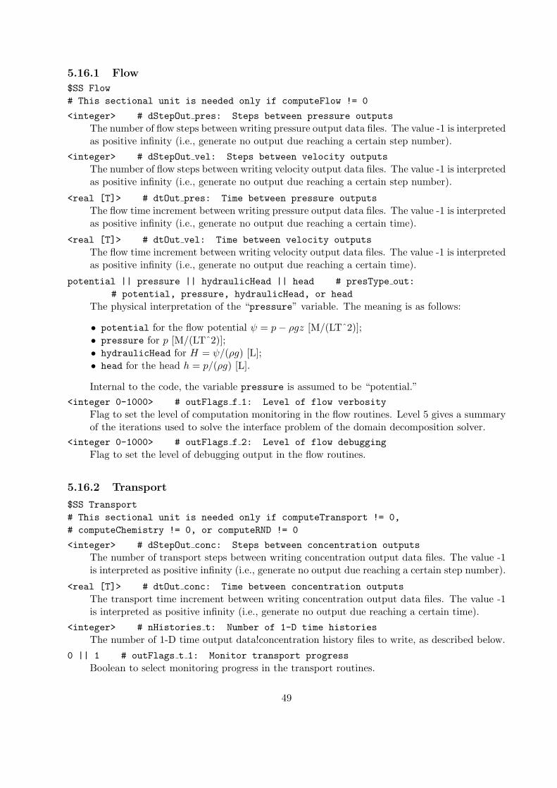
5.16.1 Flow
$SS Flow# This sectional unit is needed only if computeFlow != 0
<integer> # dStepOut pres: Steps between pressure outputsThe number of flow steps between writing pressure output data files. The value -1 is interpretedas positive infinity (i.e., generate no output due reaching a certain step number).
<integer> # dStepOut vel: Steps between velocity outputsThe number of flow steps between writing velocity output data files. The value -1 is interpretedas positive infinity (i.e., generate no output due reaching a certain step number).
<real [T]> # dtOut pres: Time between pressure outputsThe flow time increment between writing pressure output data files. The value -1 is interpretedas positive infinity (i.e., generate no output due reaching a certain time).
<real [T]> # dtOut vel: Time between velocity outputsThe flow time increment between writing velocity output data files. The value -1 is interpretedas positive infinity (i.e., generate no output due reaching a certain time).
potential || pressure || hydraulicHead || head # presType out:# potential, pressure, hydraulicHead, or head
The physical interpretation of the “pressure” variable. The meaning is as follows:
• potential for the flow potential ψ = p− ρgz [M/(LTˆ2)];• pressure for p [M/(LTˆ2)];• hydraulicHead for H = ψ/(ρg) [L];• head for the head h = p/(ρg) [L].
Internal to the code, the variable pressure is assumed to be “potential.”<integer 0-1000> # outFlags f 1: Level of flow verbosity
Flag to set the level of computation monitoring in the flow routines. Level 5 gives a summaryof the iterations used to solve the interface problem of the domain decomposition solver.
<integer 0-1000> # outFlags f 2: Level of flow debuggingFlag to set the level of debugging output in the flow routines.
5.16.2 Transport
$SS Transport# This sectional unit is needed only if computeTransport != 0,# computeChemistry != 0, or computeRND != 0
<integer> # dStepOut conc: Steps between concentration outputsThe number of transport steps between writing concentration output data files. The value -1is interpreted as positive infinity (i.e., generate no output due reaching a certain step number).
<real [T]> # dtOut conc: Time between concentration outputsThe transport time increment between writing concentration output data files. The value -1is interpreted as positive infinity (i.e., generate no output due reaching a certain time).
<integer> # nHistories t: Number of 1-D time historiesThe number of 1-D time output data!concentration history files to write, as described below.
0 || 1 # outFlags t 1: Monitor transport progressBoolean to select monitoring progress in the transport routines.
49
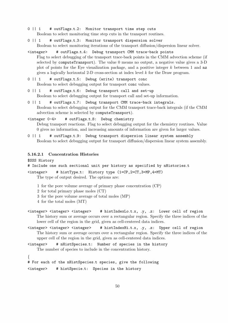
0 || 1 # outFlags t 2: Monitor transport time step cutsBoolean to select monitoring time step cuts in the transport routines.
0 || 1 # outFlags t 3: Monitor transport dispersion solverBoolean to select monitoring iterations of the transport diffusion/dispersion linear solver.
<integer> # outFlags t 4: Debug transport CMM trace-back pointsFlag to select debugging of the transport trace-back points in the CMM advection scheme (ifselected by computeTransport). The value 0 means no output, a negative value gives a 3-Dplot of points for the Eye visualization package, and a positive integer k between 1 and nzgives a logically horizontal 2-D cross-section at index level k for the Draw program.
0 || 1 # outFlags t 5: Debug (write) transport concBoolean to select debugging output for transport conc values.
0 || 1 # outFlags t 6: Debug transport call and set-upBoolean to select debugging output for transport call and set-up information.
0 || 1 # outFlags t 7: Debug transport CMM trace-back integrals.Boolean to select debugging output for the CMM transport trace-back integrals (if the CMMadvection scheme is selected by computeTransport).
<integer 0-4> # outFlags t 8: Debug chemistryDebug transport reactions. Flag to select debugging output for the chemistry routines. Value0 gives no information, and increasing amounts of information are given for larger values.
0 || 1 # outFlags t 9: Debug transport dispersion linear system assemblyBoolean to select debugging output for transport diffusion/dispersion linear system assembly.
5.16.2.1 Concentration Histories$SSS History# Include one such sectional unit per history as specified by nHistories t
<integer> # histType t: History type (1=CP,2=CT,3=MP,4=MT)The type of output desired. The options are:
1 for the pore volume average of primary phase concentration (CP)2 for total primary phase moles (CT)3 for the pore volume average of total moles (MP)4 for the total moles (MT)
<integer> <integer> <integer> # histIndexLo t x, y, z: Lower cell of regionThe history sum or average occurs over a rectangular region. Specify the three indices of thelower cell of the region in the grid, given as cell-centered data indices.
<integer> <integer> <integer> # histIndexHi t x, y, z: Upper cell of regionThe history sum or average occurs over a rectangular region. Specify the three indices of theupper cell of the region in the grid, given as cell-centered data indices.
<integer> # nHistSpecies t: Number of species in the historyThe number of species to include in the concentration history.
{# For each of the nHistSpecies t species, give the following
<integer> # histSpecie t: Species in the history
50
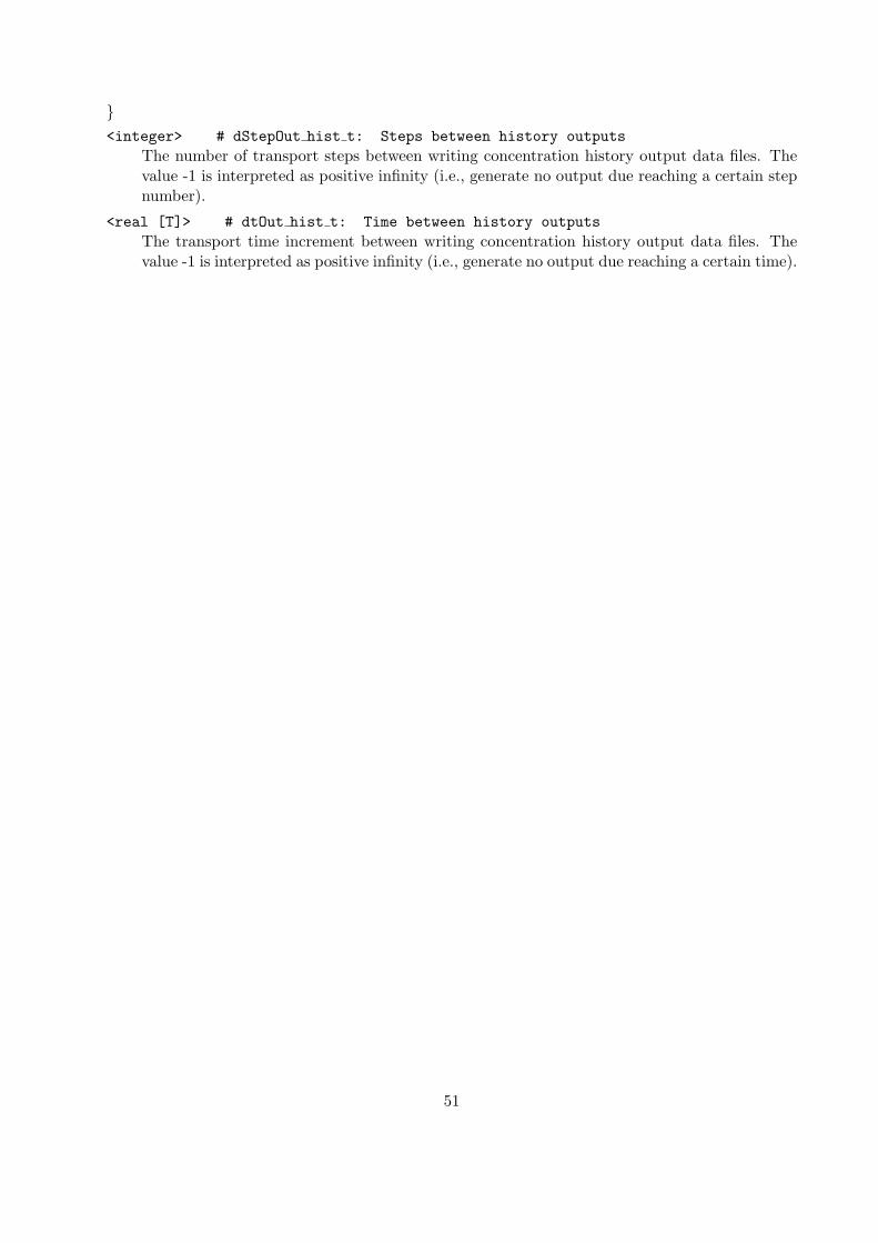
}<integer> # dStepOut hist t: Steps between history outputs
The number of transport steps between writing concentration history output data files. Thevalue -1 is interpreted as positive infinity (i.e., generate no output due reaching a certain stepnumber).
<real [T]> # dtOut hist t: Time between history outputsThe transport time increment between writing concentration history output data files. Thevalue -1 is interpreted as positive infinity (i.e., generate no output due reaching a certain time).
51
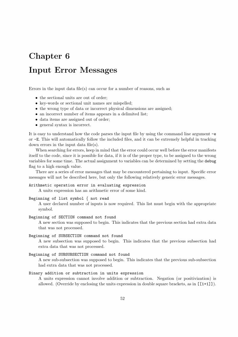
Chapter 6
Input Error Messages
Errors in the input data file(s) can occur for a number of reasons, such as
• the sectional units are out of order;• key-words or sectional unit names are mispelled;• the wrong type of data or incorrect physical dimensions are assigned;• an incorrect number of items appears in a delimited list;• data items are assigned out of order;• general syntax is incorrect.
It is easy to understand how the code parses the input file by using the command line argument -eor -E. This will automatically follow the included files, and it can be extremely helpful in trackingdown errors in the input data file(s).
When searching for errors, keep in mind that the error could occur well before the error manifestsitself to the code, since it is possible for data, if it is of the proper type, to be assigned to the wrongvariables for some time. The actual assignment to variables can be determined by setting the debugflag to a high enough value.
There are a series of error messages that may be encountered pertaining to input. Specific errormessages will not be described here, but only the following relatively generic error messages.
Arithmetic operation error in evaluating expressionA units expression has an arithmetic error of some kind.
Beginning of list symbol { not readA user declared number of inputs is now required. This list must begin with the appropriatesymbol.
Beginning of SECTION command not foundA new section was supposed to begin. This indicates that the previous section had extra datathat was not processed.
Beginning of SUBSECTION command not foundA new subsection was supposed to begin. This indicates that the previous subsection hadextra data that was not processed.
Beginning of SUBSUBSECTION command not foundA new sub-subsection was supposed to begin. This indicates that the previous sub-subsectionhad extra data that was not processed.
Binary addition or subtraction in units expressionA units expression cannot involve addition or subtraction. Negation (or positivization) isallowed. (Override by enclosing the units expression in double square brackets, as in [[1+1]]).
52
End of list symbol } not foundA user declared number of inputs was required. This list must end with the appropriatesymbol. Perhaps there are too many items in the list.
Error after input file <file name> line number <number>An otherwise unspecified error occurred somewhere after the given line of the given file. Theerror may be in a subsequently included file.
Error allocating memory on processor <number>There was an exhaustion of memory (on the given processor). You can first try to reduce theamount of workspace memory asked for. If this fails, you may be able to reduce the size ofthe problem you are solving. Finally, you can try to use a machine with more memory.
Error between input file <file name> line number <number> and input file <filename> line number <number>
An otherwise unspecified error occurred somewhere between the given lines of the given files.The error may be in an intervening included file.
Error in data blockThere is an error in a numerical data block (see §4.7.2 on page 22, and also grid array in §4.7.3on page 22). Perhaps the data block has the wrong number of items.
Error in input file <file name> before line number <number>An otherwise unspecified error occurred somewhere before the given line of the given file. Theerror may be in a previously included file. This message may be preceded by a more specificerror message.
Error in input file <file name> on line number <number>An otherwise unspecified error occurred on the given line of the given file. This message maybe preceded by a more specific error message. The item read was not of the appropriate typeto continue (e.g., an integer was expected, but a real number was found). The actual errorcould be well before this point in the file(s).
Error on processor <number>An unspecified error occurred on the given processor.
Error opening input file <file name>The given file was not able to be opened. Perhaps it is misspelled or there is an error in thedirectory tree path to the file.
Expression has nonnested parenthesesA units expression cannot have nonnested parentheses.
Grid array expectedA grid array (see §4.7.3 on page 22) was expected but not found. Perhaps a begin list symbol‘{’ was left out.
Key not found: <list of words>The key-word from the given list was not found. It is likely missing, misspelled, or out oforder.
Premature beginning of SECTION command foundA new section was begun before the last one was finished.
Premature beginning of SUBSECTION command foundA new subsection was begun before the last one was finished.
53
Premature beginning of SUBSUBSECTION command foundA new sub-subsection was begun before the last one was finished.
Premature end of dataThe data file ended before all appropriate data was read and processed.
Section key not found: <list of words>The section name from the given list was not found. It is likely missing, misspelled, or out oforder.
Sorry, there is an error in the computer codeRefer the problem to someone who can debug the code. This error message occurs generallyonly for errors that are relatively straightforward to resolve.
Subsection key not found: <list of words>The subsection name from the given list was not found. It is likely missing, misspelled, or outof order.
Subsubsection key not found: <list of words>The sub-subsection name from the given list was not found. It is likely missing, misspelled,or out of order.
Too many nested include files: maximum <number> allowedWhile there is no limit on the number of files that may be included, there is a maximumnumber that may be nested. Try to finish a file before calling for succeeding files, or have thecode recompiled with a greater number of nesting levels allowed.
Unit expression errorA units expression has an otherwise unspecified error.
Unit expression has the wrong dimensionsA units expression has the wrong physical dimensions. (Override by enclosing the units ex-pression in double square brackets, as in [[2]])
Units expression improperly formed or unknown unitA units expression is improperly formed. It is possible that an unknown unit was given, andthe expression became confused.
Units expression is not positiveA units expression is not positive. (Override by enclosing the units expression in double squarebrackets, as in [[-1]]).
Units expression is too longA units expression is too long. You must shorten it, or work out the conversion factor yourself.
Unknown $ commandThe command name was misspelled or the desired command is not supported.
Unknown unitA units expression has an unknown unit, or perhaps it was misspelled. The command lineargument -u can be used to obtain a list of supported units. New unit names and values canbe added to the code and then it can be recompiled; otherwise, the numerical value of a unit(in the base units) can be used together with the double square bracket notation.
Unmatched end comment commandAn $END COMMENT command appeared without a matching $BEGIN COMMENT command.
54
Unsupported input optionThe requested option is not supported. Try another option. To determine the supportedoptions, use this manual (or perhaps the command line argument -t to display the typenumbers of various options).
55
Chapter 7
The Output Data Files
The user may write output data files, as described in the chapter on input (Chapter 5). These filesmay be 3-D in space or 1-D in time.
The user may also write various other files for testing and debugging purposes, as described inthe chapter on input.
7.1 Data that is 3-D in space
One can write 3-D files of the pressure, velocities, and concentrations. These files are formattedso that they can be viewed directly with the graphics package Eye or Tecplot, or the raw data isgiven, depending on the setting of outFormat3D.
These 3-D file names have the structure “data.number”. Here, “data” is one of the following:
pres for pressure data;vel for vector velocity data;velx for x-velocity data;vely for y-velocity data;velz for z-velocity data;conc? for concentration data ofthe ‘?’th component (or a range of components).
There may be an appropriate graphics package extension appended to the file name. Only a singlevector velocity file or 3 component velocity files will appear, as is appropriate for the graphicspackage. The “number” is sequential, and corresponds to the respective step number and timeentry in the file presTime, velTime, or concTime, for pressure, velocity, or concentration data,respectively. The grid will be stored in the file grid.000 if the graphics package supports a separategrid file; otherwise, the grid is stored in each individual output data file.
See the documentation on Eye and Tecplot for information on the format of these files. Both ofthese formats represent all data on the same grid, that consists of the centers of the cells (not thegrid points!), the centers of the boundary faces, the centers of the boundary edges, and the eightcorners of the domain. Thus, the output grid covers the same domain as the input grid; however,the input and output grids contain different points. Pressure and concentration data is cell-centereddata, so in the output file, each cell center data value is associated to the appropriate point of theoutput grid (in the interior of the domain). On the boundary of the domain, the output grid pointsthat are face centers of the input grid have associated with them the data value of the adjacentcell. The other output grid points are associated to averages of nearby boundary data values. Thisprocedure is used so that no false maxima or minima are represented in the output files; however,this has the effect that any visual rendering may appear to be a bit too regular near the boundary.The velocities are not strictly cell-centered; for example, the x velocity velX is face centered in x
56
and cell-centered in y and z. Each cell centered value is obtained as the average of the two facecentered values of the cell, and the boundary values are either given or derived as in the case ofcell-centered data.
The Eye format is about as compact as possible. The grid is stored only once in the grid file, andeach data file contains a single data item (pressure, velocity component, or species concentration).Thus, the storage is minimized, but the number of files is maximized.
The raw data format is as compact as possible. No grid is produced, and each data file containsa single data item (pressure, velocity component, or species concentration). The order followsthe logically rectangular structure of the grid, and is given with the x coordinate varying mostrapidly, then y, and finally z (as in Fortran). All files contain cell-centered data and are of size(nx,ny,nz), except the velocity files, which contain face-centered data (e.g., the x velocity file isof size (nx+1,ny,nz)).
7.2 Data that is 1-D in time
One can write 1-D files of the concentration history of one or more species over a fixed region ofspace. These files are formatted so that they can be viewed directly with the graphics packageTecplot, as set by outFormat1D.
These 1-D file names begin with “concHist”, have the number of the history, and then twoletters describing the type of data recorded. More specifically, the names are one of
concHist?CP for the pore volume average of primary phase concentration of species m:∑n
φncm,nVn/∑n
φnVn,
concHist?CT for the pore volume average of total moles (flowing and sorbed) of species m:∑n
(φn + αmσm,n)cm,nVn/∑n
φnVn,
concHist?MP for total primary phase moles of species m:∑n
φncm,nVn
concHist?MT for the total moles (flowing and sorbed) of species m:∑n
(φn + αmσm,n)cm,nVn,
where the ‘?’ is the history number, and Vn is the volume of the nth grid element of the fixedregion. A final “i,j,k” or “,i,j,k-i,j,k” gives the cell-centered data index numbers of the fixedgrid cell or range of cells (histIndexLo t x, histIndexLo t y, histIndexLo t z and, if different,histIndexHi t x, histIndexHi t y, histIndexHi t z).
See the documentation on Tecplot for information on the format of these files.
57
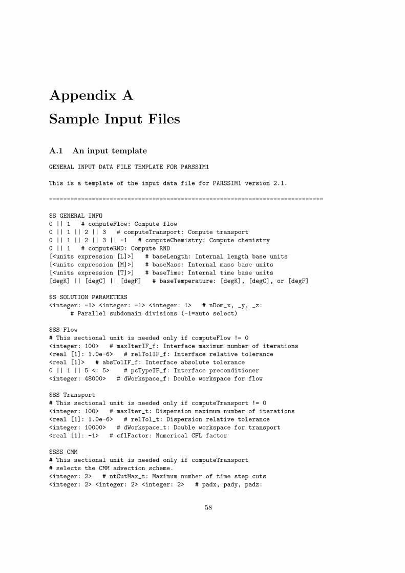
Appendix A
Sample Input Files
A.1 An input template
GENERAL INPUT DATA FILE TEMPLATE FOR PARSSIM1
This is a template of the input data file for PARSSIM1 version 2.1.
=============================================================================
$S GENERAL INFO0 || 1 # computeFlow: Compute flow0 || 1 || 2 || 3 # computeTransport: Compute transport0 || 1 || 2 || 3 || -1 # computeChemistry: Compute chemistry0 || 1 # computeRND: Compute RND[<units expression [L]>] # baseLength: Internal length base units[<units expression [M]>] # baseMass: Internal mass base units[<units expression [T]>] # baseTime: Internal time base units[degK] || [degC] || [degF] # baseTemperature: [degK], [degC], or [degF]
$S SOLUTION PARAMETERS<integer: -1> <integer: -1> <integer: 1> # nDom_x, _y, _z:
# Parallel subdomain divisions (-1=auto select)
$SS Flow# This sectional unit is needed only if computeFlow != 0<integer: 100> # maxIterIF_f: Interface maximum number of iterations<real [1]: 1.0e-6> # relTolIF_f: Interface relative tolerance<real [1]> # absTolIF_f: Interface absolute tolerance0 || 1 || 5 <: 5> # pcTypeIF_f: Interface preconditioner<integer: 48000> # dWorkspace_f: Double workspace for flow
$SS Transport# This sectional unit is needed only if computeTransport != 0<integer: 100> # maxIter_t: Dispersion maximum number of iterations<real [1]: 1.0e-6> # relTol_t: Dispersion relative tolerance<integer: 10000> # dWorkspace_t: Double workspace for transport<real [1]: -1> # cflFactor: Numerical CFL factor
$SSS CMM# This sectional unit is needed only if computeTransport# selects the CMM advection scheme.<integer: 2> # ntCutMax_t: Maximum number of time step cuts<integer: 2> <integer: 2> <integer: 2> # padx, pady, padz:
58
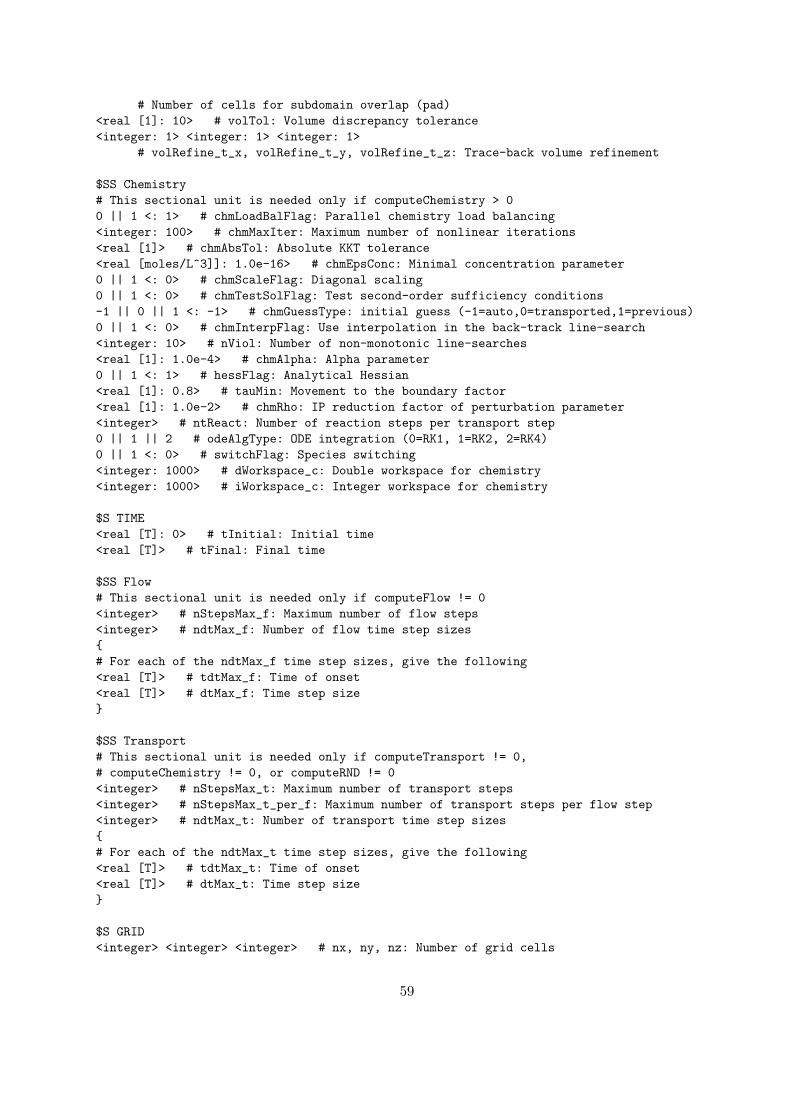
# Number of cells for subdomain overlap (pad)<real [1]: 10> # volTol: Volume discrepancy tolerance<integer: 1> <integer: 1> <integer: 1>
# volRefine_t_x, volRefine_t_y, volRefine_t_z: Trace-back volume refinement
$SS Chemistry# This sectional unit is needed only if computeChemistry > 00 || 1 <: 1> # chmLoadBalFlag: Parallel chemistry load balancing<integer: 100> # chmMaxIter: Maximum number of nonlinear iterations<real [1]> # chmAbsTol: Absolute KKT tolerance<real [moles/L^3]]: 1.0e-16> # chmEpsConc: Minimal concentration parameter0 || 1 <: 0> # chmScaleFlag: Diagonal scaling0 || 1 <: 0> # chmTestSolFlag: Test second-order sufficiency conditions-1 || 0 || 1 <: -1> # chmGuessType: initial guess (-1=auto,0=transported,1=previous)0 || 1 <: 0> # chmInterpFlag: Use interpolation in the back-track line-search<integer: 10> # nViol: Number of non-monotonic line-searches<real [1]: 1.0e-4> # chmAlpha: Alpha parameter0 || 1 <: 1> # hessFlag: Analytical Hessian<real [1]: 0.8> # tauMin: Movement to the boundary factor<real [1]: 1.0e-2> # chmRho: IP reduction factor of perturbation parameter<integer> # ntReact: Number of reaction steps per transport step0 || 1 || 2 # odeAlgType: ODE integration (0=RK1, 1=RK2, 2=RK4)0 || 1 <: 0> # switchFlag: Species switching<integer: 1000> # dWorkspace_c: Double workspace for chemistry<integer: 1000> # iWorkspace_c: Integer workspace for chemistry
$S TIME<real [T]: 0> # tInitial: Initial time<real [T]> # tFinal: Final time
$SS Flow# This sectional unit is needed only if computeFlow != 0<integer> # nStepsMax_f: Maximum number of flow steps<integer> # ndtMax_f: Number of flow time step sizes{# For each of the ndtMax_f time step sizes, give the following<real [T]> # tdtMax_f: Time of onset<real [T]> # dtMax_f: Time step size}
$SS Transport# This sectional unit is needed only if computeTransport != 0,# computeChemistry != 0, or computeRND != 0<integer> # nStepsMax_t: Maximum number of transport steps<integer> # nStepsMax_t_per_f: Maximum number of transport steps per flow step<integer> # ndtMax_t: Number of transport time step sizes{# For each of the ndtMax_t time step sizes, give the following<real [T]> # tdtMax_t: Time of onset<real [T]> # dtMax_t: Time step size}
$S GRID<integer> <integer> <integer> # nx, ny, nz: Number of grid cells
59
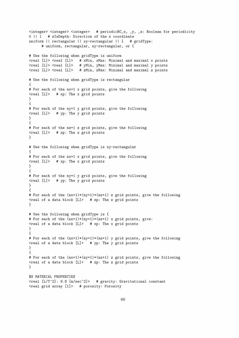
<integer> <integer> <integer> # periodicBC_x, _y, _z: Boolean for periodicity0 || 1 # zIsDepth: Direction of the z coordinateuniform || rectangular || xy-rectangular || { # gridType:
# uniform, rectangular, xy-rectangular, or {
# Use the following when gridType is uniform<real [L]> <real [L]> # xMin, xMax: Minimal and maximal x points<real [L]> <real [L]> # yMin, yMax: Minimal and maximal y points<real [L]> <real [L]> # zMin, zMax: Minimal and maximal z points
# Use the following when gridType is rectangular{# For each of the nx+1 x grid points, give the following<real [L]> # xp: The x grid points}{# For each of the ny+1 y grid points, give the following<real [L]> # yp: The y grid points}{# For each of the nz+1 z grid points, give the following<real [L]> # zp: The z grid points}
# Use the following when gridType is xy-rectangular{# For each of the nx+1 x grid points, give the following<real [L]> # xp: The x grid points}{# For each of the ny+1 y grid points, give the following<real [L]> # yp: The y grid points}{# For each of the (nx+1)*(ny+1)*(nz+1) z grid points, give the following<real of a data block [L]> # zp: The z grid points}
# Use the following when gridType is {# For each of the (nx+1)*(ny+1)*(nz+1) x grid points, give:<real of a data block [L]> # xp: The x grid points}{# For each of the (nx+1)*(ny+1)*(nz+1) y grid points, give the following<real of a data block [L]> # yp: The y grid points}{# For each of the (nx+1)*(ny+1)*(nz+1) z grid points, give the following<real of a data block [L]> # zp: The z grid points}
$S MATERIAL PROPERTIES<real [L/T^2]: 9.8 [m/sec^2]> # gravity: Gravitational constant<real grid array [1]> # porosity: Porosity
60
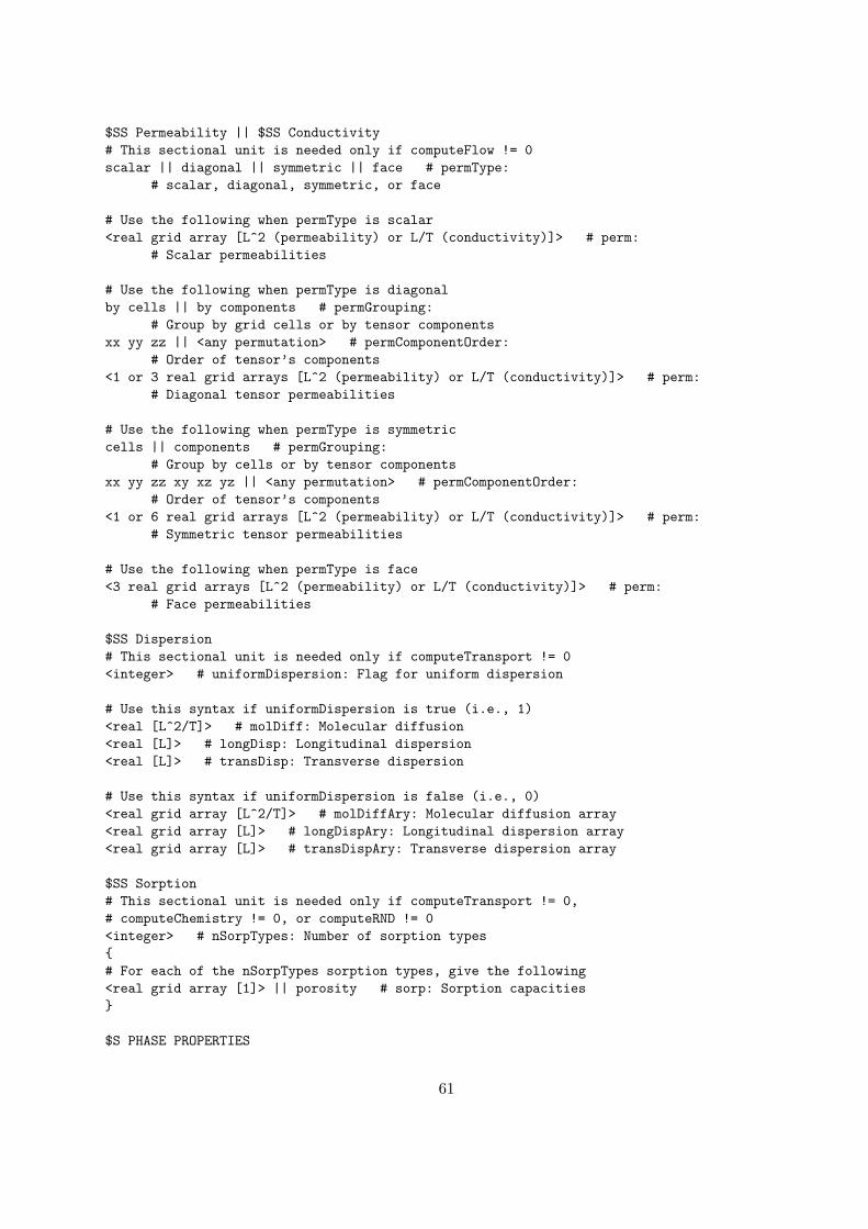
$SS Permeability || $SS Conductivity# This sectional unit is needed only if computeFlow != 0scalar || diagonal || symmetric || face # permType:
# scalar, diagonal, symmetric, or face
# Use the following when permType is scalar<real grid array [L^2 (permeability) or L/T (conductivity)]> # perm:
# Scalar permeabilities
# Use the following when permType is diagonalby cells || by components # permGrouping:
# Group by grid cells or by tensor componentsxx yy zz || <any permutation> # permComponentOrder:
# Order of tensor’s components<1 or 3 real grid arrays [L^2 (permeability) or L/T (conductivity)]> # perm:
# Diagonal tensor permeabilities
# Use the following when permType is symmetriccells || components # permGrouping:
# Group by cells or by tensor componentsxx yy zz xy xz yz || <any permutation> # permComponentOrder:
# Order of tensor’s components<1 or 6 real grid arrays [L^2 (permeability) or L/T (conductivity)]> # perm:
# Symmetric tensor permeabilities
# Use the following when permType is face<3 real grid arrays [L^2 (permeability) or L/T (conductivity)]> # perm:
# Face permeabilities
$SS Dispersion# This sectional unit is needed only if computeTransport != 0<integer> # uniformDispersion: Flag for uniform dispersion
# Use this syntax if uniformDispersion is true (i.e., 1)<real [L^2/T]> # molDiff: Molecular diffusion<real [L]> # longDisp: Longitudinal dispersion<real [L]> # transDisp: Transverse dispersion
# Use this syntax if uniformDispersion is false (i.e., 0)<real grid array [L^2/T]> # molDiffAry: Molecular diffusion array<real grid array [L]> # longDispAry: Longitudinal dispersion array<real grid array [L]> # transDispAry: Transverse dispersion array
$SS Sorption# This sectional unit is needed only if computeTransport != 0,# computeChemistry != 0, or computeRND != 0<integer> # nSorpTypes: Number of sorption types{# For each of the nSorpTypes sorption types, give the following<real grid array [1]> || porosity # sorp: Sorption capacities}
$S PHASE PROPERTIES
61
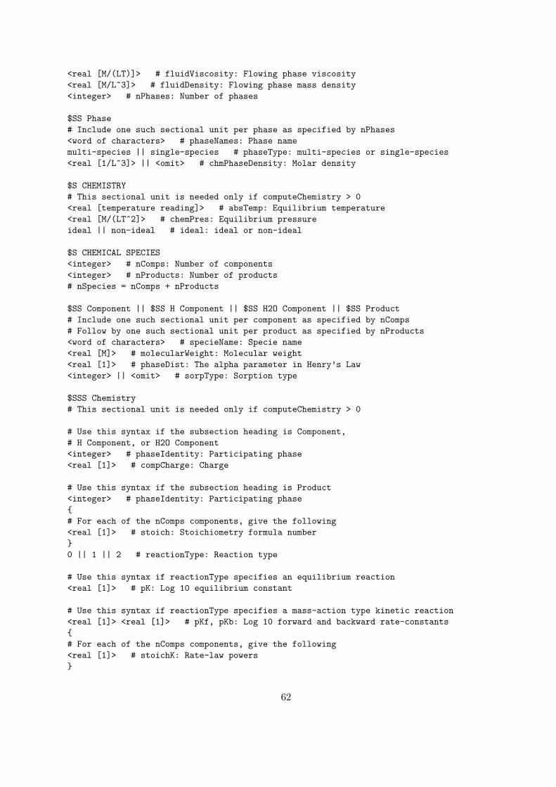
<real [M/(LT)]> # fluidViscosity: Flowing phase viscosity<real [M/L^3]> # fluidDensity: Flowing phase mass density<integer> # nPhases: Number of phases
$SS Phase# Include one such sectional unit per phase as specified by nPhases<word of characters> # phaseNames: Phase namemulti-species || single-species # phaseType: multi-species or single-species<real [1/L^3]> || <omit> # chmPhaseDensity: Molar density
$S CHEMISTRY# This sectional unit is needed only if computeChemistry > 0<real [temperature reading]> # absTemp: Equilibrium temperature<real [M/(LT^2]> # chemPres: Equilibrium pressureideal || non-ideal # ideal: ideal or non-ideal
$S CHEMICAL SPECIES<integer> # nComps: Number of components<integer> # nProducts: Number of products# nSpecies = nComps + nProducts
$SS Component || $SS H Component || $SS H2O Component || $SS Product# Include one such sectional unit per component as specified by nComps# Follow by one such sectional unit per product as specified by nProducts<word of characters> # specieName: Specie name<real [M]> # molecularWeight: Molecular weight<real [1]> # phaseDist: The alpha parameter in Henry’s Law<integer> || <omit> # sorpType: Sorption type
$SSS Chemistry# This sectional unit is needed only if computeChemistry > 0
# Use this syntax if the subsection heading is Component,# H Component, or H2O Component<integer> # phaseIdentity: Participating phase<real [1]> # compCharge: Charge
# Use this syntax if the subsection heading is Product<integer> # phaseIdentity: Participating phase{# For each of the nComps components, give the following<real [1]> # stoich: Stoichiometry formula number}0 || 1 || 2 # reactionType: Reaction type
# Use this syntax if reactionType specifies an equilibrium reaction<real [1]> # pK: Log 10 equilibrium constant
# Use this syntax if reactionType specifies a mass-action type kinetic reaction<real [1]> <real [1]> # pKf, pKb: Log 10 forward and backward rate-constants{# For each of the nComps components, give the following<real [1]> # stoichK: Rate-law powers}
62

# Use this syntax if reactionType specifies a monod type kinetic reaction<real [1]> <real [1]: -99> # pKf, pKb: Log 10 forward & backward rate-constants{# For each of the nComps components, give the following<real [1]> # stoichK: Rate-law powers}{# For each of the nComps components, give the following<real [1]> # halfSatConst: Half saturation constants}
$S MISCIBLE DISPLACEMENT# This sectional unit is needed only if computeFlow != 0 and# computeTransport != 0, computeChemistry != 0, or computeRND != 00 || 1 # modelMiscDisp: Miscible displacement model
# Use the following when modelMiscDisp selects# the quarter power mixing rule{# For each of the nSpecies species, give the following<real [1]> # viscosityRatio: Viscosity ratio}
$S RADIONUCLIDE DECAY# This sectional unit is needed only if computeRND != 0<integer> # nChains: Number of RND chains
$SS Chain# Include one such sectional unit per chain as specified by nChains<integer> # chainLen: Length of chainlinear || branching # chainType: linear or branching{# For each of the chainLen species, give the following<integer> # specieNumber: Specie number<real [T]> # halfLife: Half-life<omit> || <real [1]> ... # branchRatios: Branch ratios}
$S SPECIALIZED REACTIONS# This sectional unit is needed only if computeChemistry < 0<integer> # rxn_nComps: Number of component species in reactions{# For each of the rxn_nComps component species, give the following<integer> # rxn_comp: Species number of the next reaction component}<integer> # rxn_nMicroSteps: Number of reaction micro steps<double [1]> # rxn_tolerance: Convergence tolerance parameter<integer> # rxn_nDParams: Number of real parameters for user’s rxn fcns{# For each of the rxn_nDParams real parameters, give the following<real [1]> # rxn_dParams: Real parameter}<integer> # rxn_nIParams: Number of integer parameters for user’s rxn fcns
63
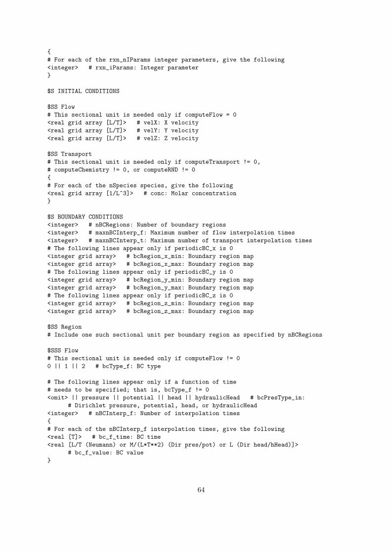
{# For each of the rxn_nIParams integer parameters, give the following<integer> # rxn_iParams: Integer parameter}
$S INITIAL CONDITIONS
$SS Flow# This sectional unit is needed only if computeFlow = 0<real grid array [L/T]> # velX: X velocity<real grid array [L/T]> # velY: Y velocity<real grid array [L/T]> # velZ: Z velocity
$SS Transport# This sectional unit is needed only if computeTransport != 0,# computeChemistry != 0, or computeRND != 0{# For each of the nSpecies species, give the following<real grid array [1/L^3]> # conc: Molar concentration}
$S BOUNDARY CONDITIONS<integer> # nBCRegions: Number of boundary regions<integer> # maxnBCInterp_f: Maximum number of flow interpolation times<integer> # maxnBCInterp_t: Maximum number of transport interpolation times# The following lines appear only if periodicBC_x is 0<integer grid array> # bcRegion_x_min: Boundary region map<integer grid array> # bcRegion_x_max: Boundary region map# The following lines appear only if periodicBC_y is 0<integer grid array> # bcRegion_y_min: Boundary region map<integer grid array> # bcRegion_y_max: Boundary region map# The following lines appear only if periodicBC_z is 0<integer grid array> # bcRegion_z_min: Boundary region map<integer grid array> # bcRegion_z_max: Boundary region map
$SS Region# Include one such sectional unit per boundary region as specified by nBCRegions
$SSS Flow# This sectional unit is needed only if computeFlow != 00 || 1 || 2 # bcType_f: BC type
# The following lines appear only if a function of time# needs to be specified; that is, bcType_f != 0<omit> || pressure || potential || head || hydraulicHead # bcPresType_in:
# Dirichlet pressure, potential, head, or hydraulicHead<integer> # nBCInterp_f: Number of interpolation times{# For each of the nBCInterp_f interpolation times, give the following<real [T]> # bc_f_time: BC time<real [L/T (Neumann) or M/(L*T**2) (Dir pres/pot) or L (Dir head/hHead)]>
# bc_f_value: BC value}
64
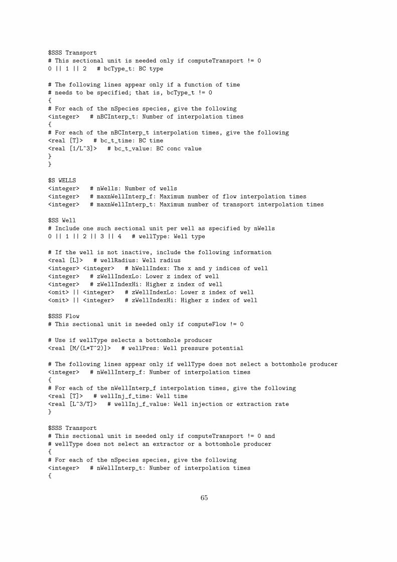
$SSS Transport# This sectional unit is needed only if computeTransport != 00 || 1 || 2 # bcType_t: BC type
# The following lines appear only if a function of time# needs to be specified; that is, bcType_t != 0{# For each of the nSpecies species, give the following<integer> # nBCInterp_t: Number of interpolation times{# For each of the nBCInterp_t interpolation times, give the following<real [T]> # bc_t_time: BC time<real [1/L^3]> # bc_t_value: BC conc value}}
$S WELLS<integer> # nWells: Number of wells<integer> # maxnWellInterp_f: Maximum number of flow interpolation times<integer> # maxnWellInterp_t: Maximum number of transport interpolation times
$SS Well# Include one such sectional unit per well as specified by nWells0 || 1 || 2 || 3 || 4 # wellType: Well type
# If the well is not inactive, include the following information<real [L]> # wellRadius: Well radius<integer> <integer> # hWellIndex: The x and y indices of well<integer> # zWellIndexLo: Lower z index of well<integer> # zWellIndexHi: Higher z index of well<omit> || <integer> # zWellIndexLo: Lower z index of well<omit> || <integer> # zWellIndexHi: Higher z index of well
$SSS Flow# This sectional unit is needed only if computeFlow != 0
# Use if wellType selects a bottomhole producer<real [M/(L*T^2)]> # wellPres: Well pressure potential
# The following lines appear only if wellType does not select a bottomhole producer<integer> # nWellInterp_f: Number of interpolation times{# For each of the nWellInterp_f interpolation times, give the following<real [T]> # wellInj_f_time: Well time<real [L^3/T]> # wellInj_f_value: Well injection or extraction rate}
$SSS Transport# This sectional unit is needed only if computeTransport != 0 and# wellType does not select an extractor or a bottomhole producer{# For each of the nSpecies species, give the following<integer> # nWellInterp_t: Number of interpolation times{
65
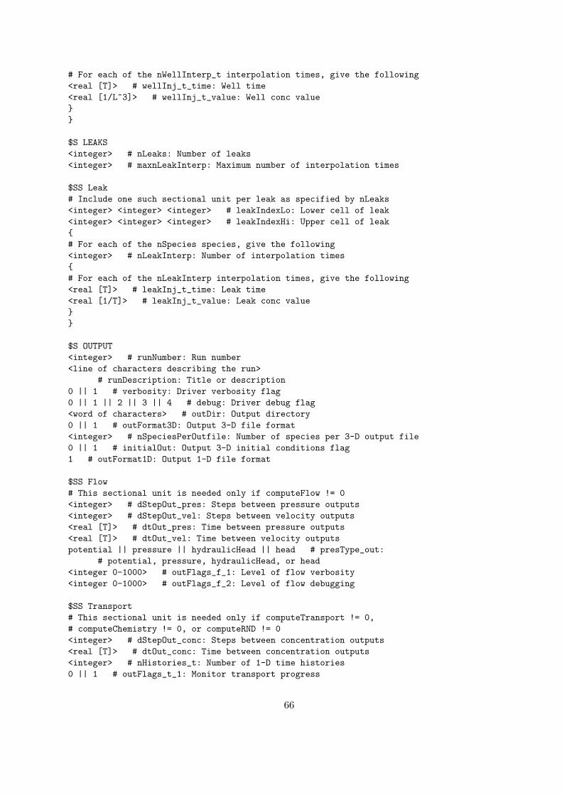
# For each of the nWellInterp_t interpolation times, give the following<real [T]> # wellInj_t_time: Well time<real [1/L^3]> # wellInj_t_value: Well conc value}}
$S LEAKS<integer> # nLeaks: Number of leaks<integer> # maxnLeakInterp: Maximum number of interpolation times
$SS Leak# Include one such sectional unit per leak as specified by nLeaks<integer> <integer> <integer> # leakIndexLo: Lower cell of leak<integer> <integer> <integer> # leakIndexHi: Upper cell of leak{# For each of the nSpecies species, give the following<integer> # nLeakInterp: Number of interpolation times{# For each of the nLeakInterp interpolation times, give the following<real [T]> # leakInj_t_time: Leak time<real [1/T]> # leakInj_t_value: Leak conc value}}
$S OUTPUT<integer> # runNumber: Run number<line of characters describing the run>
# runDescription: Title or description0 || 1 # verbosity: Driver verbosity flag0 || 1 || 2 || 3 || 4 # debug: Driver debug flag<word of characters> # outDir: Output directory0 || 1 # outFormat3D: Output 3-D file format<integer> # nSpeciesPerOutfile: Number of species per 3-D output file0 || 1 # initialOut: Output 3-D initial conditions flag1 # outFormat1D: Output 1-D file format
$SS Flow# This sectional unit is needed only if computeFlow != 0<integer> # dStepOut_pres: Steps between pressure outputs<integer> # dStepOut_vel: Steps between velocity outputs<real [T]> # dtOut_pres: Time between pressure outputs<real [T]> # dtOut_vel: Time between velocity outputspotential || pressure || hydraulicHead || head # presType_out:
# potential, pressure, hydraulicHead, or head<integer 0-1000> # outFlags_f_1: Level of flow verbosity<integer 0-1000> # outFlags_f_2: Level of flow debugging
$SS Transport# This sectional unit is needed only if computeTransport != 0,# computeChemistry != 0, or computeRND != 0<integer> # dStepOut_conc: Steps between concentration outputs<real [T]> # dtOut_conc: Time between concentration outputs<integer> # nHistories_t: Number of 1-D time histories0 || 1 # outFlags_t_1: Monitor transport progress
66
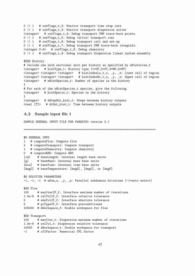
0 || 1 # outFlags_t_2: Monitor transport time step cuts0 || 1 # outFlags_t_3: Monitor transport dispersion solver<integer> # outFlags_t_4: Debug transport CMM trace-back points0 || 1 # outFlags_t_5: Debug (write) transport conc0 || 1 # outFlags_t_6: Debug transport call and set-up0 || 1 # outFlags_t_7: Debug transport CMM trace-back integrals.<integer 0-4> # outFlags_t_8: Debug chemistry0 || 1 # outFlags_t_9: Debug transport dispersion linear system assembly
$SSS History# Include one such sectional unit per history as specified by nHistories_t<integer> # histType_t: History type (1=CP,2=CT,3=MP,4=MT)<integer> <integer> <integer> # histIndexLo_t_x, _y, _z: Lower cell of region<integer> <integer> <integer> # histIndexHi_t_x, _y, _z: Upper cell of region<integer> # nHistSpecies_t: Number of species in the history{# For each of the nHistSpecies_t species, give the following<integer> # histSpecie_t: Species in the history}<integer> # dStepOut_hist_t: Steps between history outputs<real [T]> # dtOut_hist_t: Time between history outputs
A.2 Sample input file 1
SAMPLE GENERAL INPUT FILE FOR PARSSIM1 version 2.1
=============================================================================
$S GENERAL INFO1 # computeFlow: Compute flow2 # computeTransport: Compute transport1 # computeChemistry: Compute chemistry0 # computeRND: Compute RND[cm] # baseLength: Internal length base units[g] # baseMass: Internal mass base units[min] # baseTime: Internal time base units[degC] # baseTemperature: [degK], [degC], or [degF]
$S SOLUTION PARAMETERS-1, -1, -1 # nDom_x, _y, _z: Parallel subdomain divisions (-1=auto select)
$SS Flow100 # maxIterIF_f: Interface maximum number of iterations1.0e-6 # relTolIF_f: Interface relative tolerance0 # absTolIF_f: Interface absolute tolerance5 # pcTypeIF_f: Interface preconditioner100000 # dWorkspace_f: Double workspace for flow
$SS Transport100 # maxIter_t: Dispersion maximum number of iterations1.0e-6 # relTol_t: Dispersion relative tolerance10000 # dWorkspace_t: Double workspace for transport-1 # cflFactor: Numerical CFL factor
67
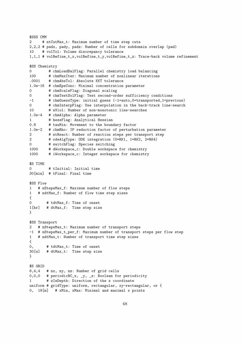
$SSS CMM2 # ntCutMax_t: Maximum number of time step cuts2,2,2 # padx, pady, padz: Number of cells for subdomain overlap (pad)10 # volTol: Volume discrepancy tolerance1,1,1 # volRefine_t_x,volRefine_t_y,volRefine_t_z: Trace-back volume refinement
$SS Chemistry0 # chmLoadBalFlag: Parallel chemistry load balancing100 # chmMaxIter: Maximum number of nonlinear iterations.0001 # chmAbsTol: Absolute KKT tolerance1.0e-16 # chmEpsConc: Minimal concentration parameter0 # chmScaleFlag: Diagonal scaling0 # chmTestSolFlag: Test second-order sufficiency conditions-1 # chmGuessType: initial guess (-1=auto,0=transported,1=previous)0 # chmInterpFlag: Use interpolation in the back-track line-search10 # nViol: Number of non-monotonic line-searches1.0e-4 # chmAlpha: Alpha parameter1 # hessFlag: Analytical Hessian0.8 # tauMin: Movement to the boundary factor1.0e-2 # chmRho: IP reduction factor of perturbation parameter2 # ntReact: Number of reaction steps per transport step2 # odeAlgType: ODE integration (0=RK1, 1=RK2, 2=RK4)0 # switchFlag: Species switching1000 # dWorkspace_c: Double workspace for chemistry1000 # iWorkspace_c: Integer workspace for chemistry
$S TIME0 # tInitial: Initial time30[min] # tFinal: Final time
$SS Flow1 # nStepsMax_f: Maximum number of flow steps1 # ndtMax_f: Number of flow time step sizes{0 # tdtMax_f: Time of onset1[hr] # dtMax_f: Time step size}
$SS Transport2 # nStepsMax_t: Maximum number of transport steps-1 # nStepsMax_t_per_f: Maximum number of transport steps per flow step1 # ndtMax_t: Number of transport time step sizes{0, # tdtMax_t: Time of onset30[s] # dtMax_t: Time step size}
$S GRID8,4,4 # nx, ny, nz: Number of grid cells0,0,0 # periodicBC_x, _y, _z: Boolean for periodicity1 # zIsDepth: Direction of the z coordinateuniform # gridType: uniform, rectangular, xy-rectangular, or {0, 18[m] # xMin, xMax: Minimal and maximal x points
68
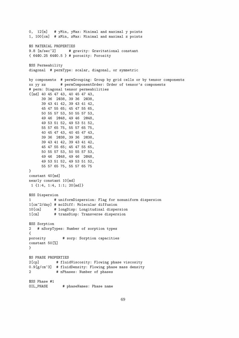
0, 12[m] # yMin, yMax: Minimal and maximal y points1, 100[cm] # zMin, zMax: Minimal and maximal z points
$S MATERIAL PROPERTIES9.8 [m/sec^2] # gravity: Gravitational constant{ [email protected] [email protected] } # porosity: Porosity
$SS Permeabilitydiagonal # permType: scalar, diagonal, or symmetric
by components # permGrouping: Group by grid cells or by tensor componentsxx yy zz # permComponentOrder: Order of tensor’s components# perm: Diagonal tensor permeabilities{[md] 40 45 47 43, 40 45 47 43,
39 36 2@38, 39 36 2@38,39 43 41 42, 39 43 41 42,45 47 55 65; 45 47 55 65,50 55 57 53, 50 55 57 53,49 46 2@48, 49 46 2@48,49 53 51 52, 49 53 51 52,55 57 65 75, 55 57 65 75,40 45 47 43, 40 45 47 43,39 36 2@38, 39 36 2@38,39 43 41 42, 39 43 41 42,45 47 55 65; 45 47 55 65,50 55 57 53, 50 55 57 53,49 46 2@48, 49 46 2@48,49 53 51 52, 49 53 51 52,55 57 65 75, 55 57 65 75
}constant 40[md]nearly constant 10[md]1 {1:4, 1:4, 1:1; 20[md]}
$SS Dispersion1 # uniformDispersion: Flag for nonuniform dispersion1[cm^2/day] # molDiff: Molecular diffusion10[cm] # longDisp: Longitudinal dispersion1[cm] # transDisp: Transverse dispersion
$SS Sorption2 # nSorpTypes: Number of sorption types{porosity # sorp: Sorption capacitiesconstant 50[%]}
$S PHASE PROPERTIES2[cp] # fluidViscosity: Flowing phase viscosity0.9[g/cm^3] # fluidDensity: Flowing phase mass density2 # nPhases: Number of phases
$SS Phase #1OIL_PHASE # phaseNames: Phase name
69
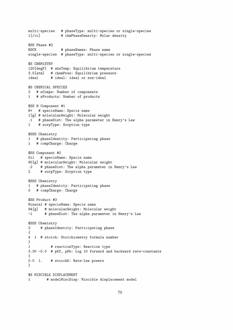
multi-species # phaseType: multi-species or single-species1[/cc] # chmPhaseDensity: Molar density
$SS Phase #2ROCK # phaseNames: Phase namesingle-species # phaseType: multi-species or single-species
$S CHEMISTRY120[degF] # absTemp: Equilibrium temperature3.5[atm] # chemPres: Equilibrium pressureideal # ideal: ideal or non-ideal
$S CHEMICAL SPECIES2 # nComps: Number of components1 # nProducts: Number of products
$SS H Component #1H+ # specieName: Specie name1[g] # molecularWeight: Molecular weight.1 # phaseDist: The alpha parameter in Henry’s Law1 # sorpType: Sorption type
$SSS Chemistry1 # phaseIdentity: Participating phase1 # compCharge: Charge
$SS Component #2Oil # specieName: Specie name90[g] # molecularWeight: Molecular weight.2 # phaseDist: The alpha parameter in Henry’s Law2 # sorpType: Sorption type
$SSS Chemistry1 # phaseIdentity: Participating phase0 # compCharge: Charge
$SS Product #3Mineral # specieName: Specie name94[g] # molecularWeight: Molecular weight-1 # phaseDist: The alpha parameter in Henry’s Law
$SSS Chemistry2 # phaseIdentity: Participating phase{4 1 # stoich: Stoichiometry formula number}1 # reactionType: Reaction type3.30 -5.0 # pKf, pKb: Log 10 forward and backward rate-constants{0.0 1. # stoichK: Rate-law powers}
$S MISCIBLE DISPLACEMENT1 # modelMiscDisp: Miscible displacement model
70
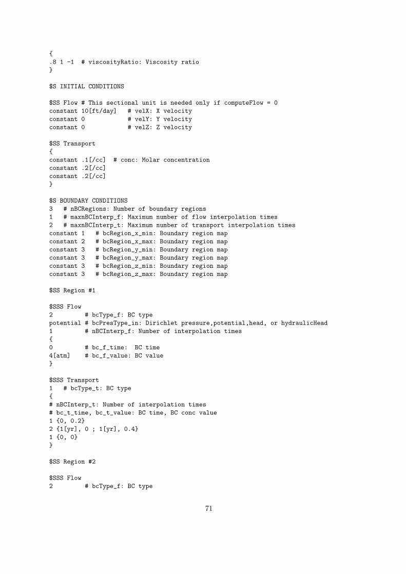
{.8 1 -1 # viscosityRatio: Viscosity ratio}
$S INITIAL CONDITIONS
$SS Flow # This sectional unit is needed only if computeFlow = 0constant 10[ft/day] # velX: X velocityconstant 0 # velY: Y velocityconstant 0 # velZ: Z velocity
$SS Transport{constant .1[/cc] # conc: Molar concentrationconstant .2[/cc]constant .2[/cc]}
$S BOUNDARY CONDITIONS3 # nBCRegions: Number of boundary regions1 # maxnBCInterp_f: Maximum number of flow interpolation times2 # maxnBCInterp_t: Maximum number of transport interpolation timesconstant 1 # bcRegion_x_min: Boundary region mapconstant 2 # bcRegion_x_max: Boundary region mapconstant 3 # bcRegion_y_min: Boundary region mapconstant 3 # bcRegion_y_max: Boundary region mapconstant 3 # bcRegion_z_min: Boundary region mapconstant 3 # bcRegion_z_max: Boundary region map
$SS Region #1
$SSS Flow2 # bcType_f: BC typepotential # bcPresType_in: Dirichlet pressure,potential,head, or hydraulicHead1 # nBCInterp_f: Number of interpolation times{0 # bc_f_time: BC time4[atm] # bc_f_value: BC value}
$SSS Transport1 # bcType_t: BC type{# nBCInterp_t: Number of interpolation times# bc_t_time, bc_t_value: BC time, BC conc value1 {0, 0.2}2 {1[yr], 0 ; 1[yr], 0.4}1 {0, 0}}
$SS Region #2
$SSS Flow2 # bcType_f: BC type
71
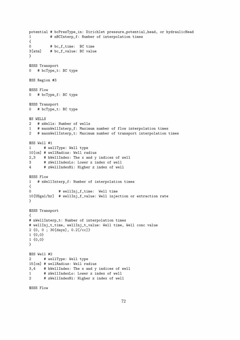
potential # bcPresType_in: Dirichlet pressure,potential,head, or hydraulicHead1 # nBCInterp_f: Number of interpolation times{0 # bc_f_time: BC time3[atm] # bc_f_value: BC value}
$SSS Transport0 # bcType_t: BC type
$SS Region #3
$SSS Flow0 # bcType_f: BC type
$SSS Transport0 # bcType_t: BC type
$S WELLS2 # nWells: Number of wells1 # maxnWellInterp_f: Maximum number of flow interpolation times2 # maxnWellInterp_t: Maximum number of transport interpolation times
$SS Well #11 # wellType: Well type10[cm] # wellRadius: Well radius2,3 # hWellIndex: The x and y indices of well3 # zWellIndexLo: Lower z index of well4 # zWellIndexHi: Higher z index of well
$SSS Flow1 # nWellInterp_f: Number of interpolation times{0 # wellInj_f_time: Well time10[USgal/hr] # wellInj_f_value: Well injection or extraction rate}
$SSS Transport{# nWellInterp_t: Number of interpolation times# wellInj_t_time, wellInj_t_value: Well time, Well conc value2 {0, 0 ; 30[days], 0.2[/cc]}1 {0,0}1 {0,0}}
$SS Well #22 # wellType: Well type15[cm] # wellRadius: Well radius3,4 # hWellIndex: The x and y indices of well1 # zWellIndexLo: Lower z index of well2 # zWellIndexHi: Higher z index of well
$SSS Flow
72
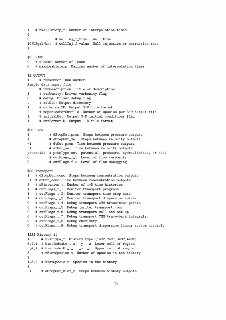
1 # nWellInterp_f: Number of interpolation times{0 # wellInj_f_time: Well time10[USgal/hr] # wellInj_f_value: Well injection or extraction rate}
$S LEAKS0 # nLeaks: Number of leaks0 # maxnLeakInterp: Maximum number of interpolation times
$S OUTPUT1 # runNumber: Run numberSample data input file
# runDescription: Title or description1 # verbosity: Driver verbosity flag0 # debug: Driver debug flag. # outDir: Output directory1 # outFormat3D: Output 3-D file format2 # nSpeciesPerOutfile: Number of species per 3-D output file1 # initialOut: Output 3-D initial conditions flag1 # outFormat1D: Output 1-D file format
$SS Flow1 # dStepOut_pres: Steps between pressure outputs1 # dStepOut_vel: Steps between velocity outputs-1 # dtOut_pres: Time between pressure outputs-1 # dtOut_vel: Time between velocity outputspotential # presType_out: potential, pressure, hydraulicHead, or head0 # outFlags_f_1: Level of flow verbosity0 # outFlags_f_2: Level of flow debugging
$SS Transport1 # dStepOut_conc: Steps between concentration outputs-1 # dtOut_conc: Time between concentration outputs3 # nHistories_t: Number of 1-D time histories1 # outFlags_t_1: Monitor transport progress1 # outFlags_t_2: Monitor transport time step cuts1 # outFlags_t_3: Monitor transport dispersion solver0 # outFlags_t_4: Debug transport CMM trace-back points0 # outFlags_t_5: Debug (write) transport conc0 # outFlags_t_6: Debug transport call and set-up0 # outFlags_t_7: Debug transport CMM trace-back integrals.0 # outFlags_t_8: Debug chemistry0 # outFlags_t_9: Debug transport dispersion linear system assembly
$SSS History #11 # histType_t: History type (1=CP,2=CT,3=MP,4=MT)5,4,1 # histIndexLo_t_x, _y, _z: Lower cell of region5,4,1 # histIndexHi_t_x, _y, _z: Upper cell of region3 # nHistSpecies_t: Number of species in the history{1,3,2 # histSpecie_t: Species in the history}-1 # dStepOut_hist_t: Steps between history outputs
73
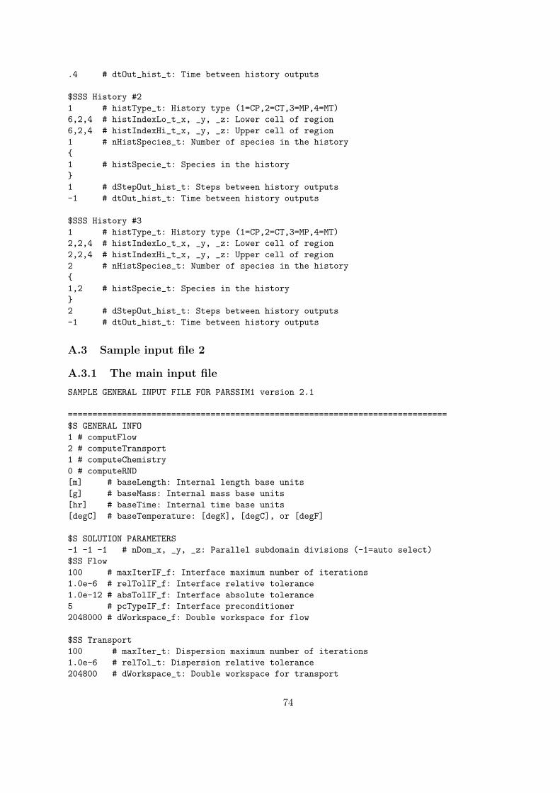
.4 # dtOut_hist_t: Time between history outputs
$SSS History #21 # histType_t: History type (1=CP,2=CT,3=MP,4=MT)6,2,4 # histIndexLo_t_x, _y, _z: Lower cell of region6,2,4 # histIndexHi_t_x, _y, _z: Upper cell of region1 # nHistSpecies_t: Number of species in the history{1 # histSpecie_t: Species in the history}1 # dStepOut_hist_t: Steps between history outputs-1 # dtOut_hist_t: Time between history outputs
$SSS History #31 # histType_t: History type (1=CP,2=CT,3=MP,4=MT)2,2,4 # histIndexLo_t_x, _y, _z: Lower cell of region2,2,4 # histIndexHi_t_x, _y, _z: Upper cell of region2 # nHistSpecies_t: Number of species in the history{1,2 # histSpecie_t: Species in the history}2 # dStepOut_hist_t: Steps between history outputs-1 # dtOut_hist_t: Time between history outputs
A.3 Sample input file 2
A.3.1 The main input file
SAMPLE GENERAL INPUT FILE FOR PARSSIM1 version 2.1
=============================================================================$S GENERAL INFO1 # computFlow2 # computeTransport1 # computeChemistry0 # computeRND[m] # baseLength: Internal length base units[g] # baseMass: Internal mass base units[hr] # baseTime: Internal time base units[degC] # baseTemperature: [degK], [degC], or [degF]
$S SOLUTION PARAMETERS-1 -1 -1 # nDom_x, _y, _z: Parallel subdomain divisions (-1=auto select)$SS Flow100 # maxIterIF_f: Interface maximum number of iterations1.0e-6 # relTolIF_f: Interface relative tolerance1.0e-12 # absTolIF_f: Interface absolute tolerance5 # pcTypeIF_f: Interface preconditioner2048000 # dWorkspace_f: Double workspace for flow
$SS Transport100 # maxIter_t: Dispersion maximum number of iterations1.0e-6 # relTol_t: Dispersion relative tolerance204800 # dWorkspace_t: Double workspace for transport
74
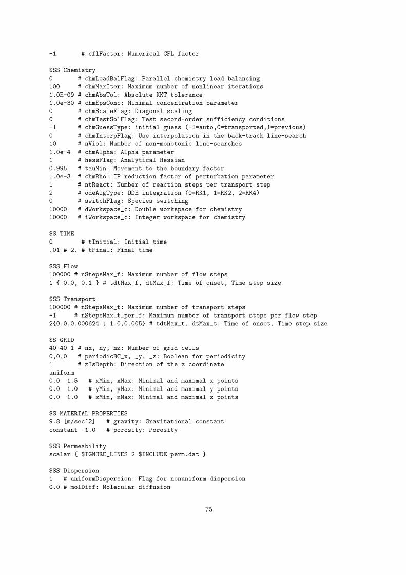
-1 # cflFactor: Numerical CFL factor
$SS Chemistry0 # chmLoadBalFlag: Parallel chemistry load balancing100 # chmMaxIter: Maximum number of nonlinear iterations1.0E-09 # chmAbsTol: Absolute KKT tolerance1.0e-30 # chmEpsConc: Minimal concentration parameter0 # chmScaleFlag: Diagonal scaling0 # chmTestSolFlag: Test second-order sufficiency conditions-1 # chmGuessType: initial guess (-1=auto,0=transported,1=previous)0 # chmInterpFlag: Use interpolation in the back-track line-search10 # nViol: Number of non-monotonic line-searches1.0e-4 # chmAlpha: Alpha parameter1 # hessFlag: Analytical Hessian0.995 # tauMin: Movement to the boundary factor1.0e-3 # chmRho: IP reduction factor of perturbation parameter1 # ntReact: Number of reaction steps per transport step2 # odeAlgType: ODE integration (0=RK1, 1=RK2, 2=RK4)0 # switchFlag: Species switching10000 # dWorkspace_c: Double workspace for chemistry10000 # iWorkspace_c: Integer workspace for chemistry
$S TIME0 # tInitial: Initial time.01 # 2. # tFinal: Final time
$SS Flow100000 # nStepsMax_f: Maximum number of flow steps1 { 0.0, 0.1 } # tdtMax_f, dtMax_f: Time of onset, Time step size
$SS Transport100000 # nStepsMax_t: Maximum number of transport steps-1 # nStepsMax_t_per_f: Maximum number of transport steps per flow step2{0.0,0.000624 ; 1.0,0.005} # tdtMax_t, dtMax_t: Time of onset, Time step size
$S GRID40 40 1 # nx, ny, nz: Number of grid cells0,0,0 # periodicBC_x, _y, _z: Boolean for periodicity1 # zIsDepth: Direction of the z coordinateuniform0.0 1.5 # xMin, xMax: Minimal and maximal x points0.0 1.0 # yMin, yMax: Minimal and maximal y points0.0 1.0 # zMin, zMax: Minimal and maximal z points
$S MATERIAL PROPERTIES9.8 [m/sec^2] # gravity: Gravitational constantconstant 1.0 # porosity: Porosity
$SS Permeabilityscalar { $IGNORE_LINES 2 $INCLUDE perm.dat }
$SS Dispersion1 # uniformDispersion: Flag for nonuniform dispersion0.0 # molDiff: Molecular diffusion
75
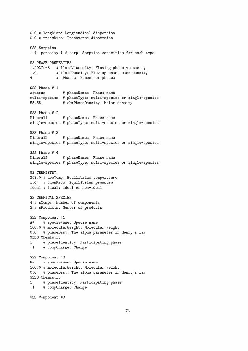
0.0 # longDisp: Longitudinal dispersion0.0 # transDisp: Transverse dispersion
$SS Sorption1 { porosity } # sorp: Sorption capacities for each type
$S PHASE PROPERTIES1.2037e-8 # fluidViscosity: Flowing phase viscosity1.0 # fluidDensity: Flowing phase mass density4 # nPhases: Number of phases
$SS Phase # 1Aqueous # phaseNames: Phase namemulti-species # phaseType: multi-species or single-species55.55 # chmPhaseDensity: Molar density
$SS Phase # 2Mineral1 # phaseNames: Phase namesingle-species # phaseType: multi-species or single-species
$SS Phase # 3Mineral2 # phaseNames: Phase namesingle-species # phaseType: multi-species or single-species
$SS Phase # 4Mineral3 # phaseNames: Phase namesingle-species # phaseType: multi-species or single-species
$S CHEMISTRY298.0 # absTemp: Equilibrium temperature1.0 # chemPres: Equilibrium pressureideal # ideal: ideal or non-ideal
$S CHEMICAL SPECIES4 # nComps: Number of components3 # nProducts: Number of products
$SS Component #1A+ # specieName: Specie name100.0 # molecularWeight: Molecular weight0.0 # phaseDist: The alpha parameter in Henry’s Law$SSS Chemistry1 # phaseIdentity: Participating phase+1 # compCharge: Charge
$SS Component #2B- # specieName: Specie name100.0 # molecularWeight: Molecular weight0.0 # phaseDist: The alpha parameter in Henry’s Law$SSS Chemistry1 # phaseIdentity: Participating phase-1 # compCharge: Charge
$SS Component #3
76
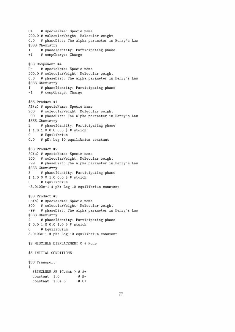
C+ # specieName: Specie name200.0 # molecularWeight: Molecular weight0.0 # phaseDist: The alpha parameter in Henry’s Law$SSS Chemistry1 # phaseIdentity: Participating phase+1 # compCharge: Charge
$SS Component #4D- # specieName: Specie name200.0 # molecularWeight: Molecular weight0.0 # phaseDist: The alpha parameter in Henry’s Law$SSS Chemistry1 # phaseIdentity: Participating phase-1 # compCharge: Charge
$SS Product #1AB(s) # specieName: Specie name200 # molecularWeight: Molecular weight-99 # phaseDist: The alpha parameter in Henry’s Law$SSS Chemistry2 # phaseIdentity: Participating phase{ 1.0 1.0 0.0 0.0 } # stoich0 # Equilibrium0.0 # pK: Log 10 equilibrium constant
$SS Product #2AC(s) # specieName: Specie name300 # molecularWeight: Molecular weight-99 # phaseDist: The alpha parameter in Henry’s Law$SSS Chemistry3 # phaseIdentity: Participating phase{ 1.0 0.0 1.0 0.0 } # stoich0 # Equilibrium-3.0103e-1 # pK: Log 10 equilibrium constant
$SS Product #3DB(s) # specieName: Specie name300 # molecularWeight: Molecular weight-99 # phaseDist: The alpha parameter in Henry’s Law$SSS Chemistry4 # phaseIdentity: Participating phase{ 0.0 1.0 0.0 1.0 } # stoich0 # Equilibrium3.0103e-1 # pK: Log 10 equilibrium constant
$S MISCIBLE DISPLACEMENT 0 # None
$S INITIAL CONDITIONS
$SS Transport{{$INCLUDE AB_IC.dat } # A+constant 1.0 # B-constant 1.0e-6 # C+
77
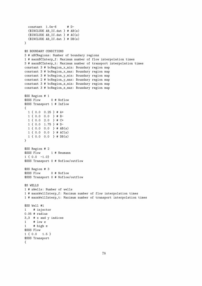
constant 1.0e-6 # D-{$INCLUDE AB_IC.dat } # AB(s){$INCLUDE AB_IC.dat } # AC(s){$INCLUDE AB_IC.dat } # DB(s)
}
$S BOUNDARY CONDITIONS3 # nBCRegions: Number of boundary regions1 # maxnBCInterp_f: Maximum number of flow interpolation times3 # maxnBCInterp_t: Maximum number of transport interpolation timesconstant 3 # bcRegion_x_min: Boundary region mapconstant 3 # bcRegion_x_max: Boundary region mapconstant 3 # bcRegion_y_min: Boundary region mapconstant 2 # bcRegion_y_max: Boundary region mapconstant 3 # bcRegion_z_min: Boundary region mapconstant 3 # bcRegion_z_max: Boundary region map
$SS Region # 1$SSS Flow 0 # Noflow$SSS Transport 1 # Inflow{1 { 0.0 0.25 } # A+1 { 0.0 0.0 } # B-1 { 0.0 2.0 } # C+1 { 0.0 1.75 } # D-1 { 0.0 0.0 } # AB(s)1 { 0.0 0.0 } # AC(s)1 { 0.0 0.0 } # DB(s)
}
$SS Region # 2$SSS Flow 1 # Neumann1 { 0.0 -1.0}$SSS Transport 0 # Noflow/outflow
$SS Region # 3$SSS Flow 0 # Noflow$SSS Transport 0 # Noflow/outflow
$S WELLS1 # nWells: Number of wells1 # maxnWellInterp_f: Maximum number of flow interpolation times1 # maxnWellInterp_t: Maximum number of transport interpolation times
$SS Well #11 # injector0.05 # radius3,3 # x and y indices1 # low z1 # high z$SSS Flow1 { 0.0 1.5 }$SSS Transport{
78
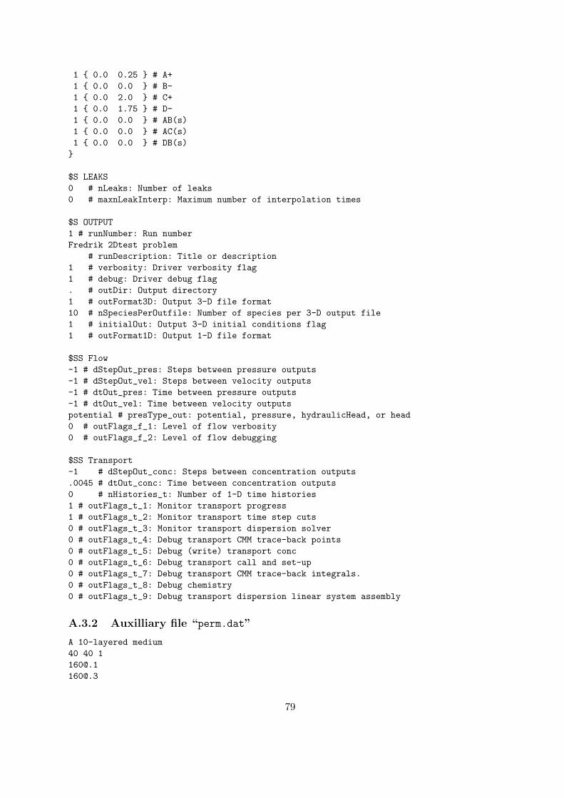
1 { 0.0 0.25 } # A+1 { 0.0 0.0 } # B-1 { 0.0 2.0 } # C+1 { 0.0 1.75 } # D-1 { 0.0 0.0 } # AB(s)1 { 0.0 0.0 } # AC(s)1 { 0.0 0.0 } # DB(s)}
$S LEAKS0 # nLeaks: Number of leaks0 # maxnLeakInterp: Maximum number of interpolation times
$S OUTPUT1 # runNumber: Run numberFredrik 2Dtest problem
# runDescription: Title or description1 # verbosity: Driver verbosity flag1 # debug: Driver debug flag. # outDir: Output directory1 # outFormat3D: Output 3-D file format10 # nSpeciesPerOutfile: Number of species per 3-D output file1 # initialOut: Output 3-D initial conditions flag1 # outFormat1D: Output 1-D file format
$SS Flow-1 # dStepOut_pres: Steps between pressure outputs-1 # dStepOut_vel: Steps between velocity outputs-1 # dtOut_pres: Time between pressure outputs-1 # dtOut_vel: Time between velocity outputspotential # presType_out: potential, pressure, hydraulicHead, or head0 # outFlags_f_1: Level of flow verbosity0 # outFlags_f_2: Level of flow debugging
$SS Transport-1 # dStepOut_conc: Steps between concentration outputs.0045 # dtOut_conc: Time between concentration outputs0 # nHistories_t: Number of 1-D time histories1 # outFlags_t_1: Monitor transport progress1 # outFlags_t_2: Monitor transport time step cuts0 # outFlags_t_3: Monitor transport dispersion solver0 # outFlags_t_4: Debug transport CMM trace-back points0 # outFlags_t_5: Debug (write) transport conc0 # outFlags_t_6: Debug transport call and set-up0 # outFlags_t_7: Debug transport CMM trace-back integrals.0 # outFlags_t_8: Debug chemistry0 # outFlags_t_9: Debug transport dispersion linear system assembly
A.3.2 Auxilliary file “perm.dat”
A 10-layered medium40 40 [email protected]@.3
79
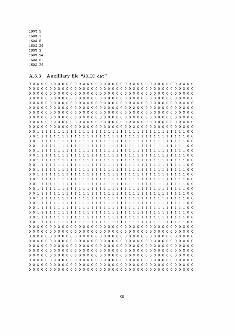
[email protected]@[email protected]@[email protected]@[email protected]@.24
A.3.3 Auxilliary file “AB IC.dat”
0 0 0 0 0 0 0 0 0 0 0 0 0 0 0 0 0 0 0 0 0 0 0 0 0 0 0 0 0 0 0 0 0 0 0 0 0 0 0 00 0 0 0 0 0 0 0 0 0 0 0 0 0 0 0 0 0 0 0 0 0 0 0 0 0 0 0 0 0 0 0 0 0 0 0 0 0 0 00 0 0 0 0 0 0 0 0 0 0 0 0 0 0 0 0 0 0 0 0 0 0 0 0 0 0 0 0 0 0 0 0 0 0 0 0 0 0 00 0 0 0 0 0 0 0 0 0 0 0 0 0 0 0 0 0 0 0 0 0 0 0 0 0 0 0 0 0 0 0 0 0 0 0 0 0 0 00 0 0 0 0 0 0 0 0 0 0 0 0 0 0 0 0 0 0 0 0 0 0 0 0 0 0 0 0 0 0 0 0 0 0 0 0 0 0 00 0 0 0 0 0 0 0 0 0 0 0 0 0 0 0 0 0 0 0 0 0 0 0 0 0 0 0 0 0 0 0 0 0 0 0 0 0 0 00 0 0 0 0 0 0 0 0 0 0 0 0 0 0 0 0 0 0 0 0 0 0 0 0 0 0 0 0 0 0 0 0 0 0 0 0 0 0 00 0 0 0 0 0 0 0 0 0 0 0 0 0 0 0 0 0 0 0 0 0 0 0 0 0 0 0 0 0 0 0 0 0 0 0 0 0 0 00 0 0 0 0 0 0 0 0 0 0 0 0 0 0 0 0 0 0 0 0 0 0 0 0 0 0 0 0 0 0 0 0 0 0 0 0 0 0 00 0 0 0 0 0 0 0 0 0 0 0 0 0 0 0 0 0 0 0 0 0 0 0 0 0 0 0 0 0 0 0 0 0 0 0 0 0 0 00 0 1 1 1 1 1 1 1 1 1 1 1 1 1 1 1 1 1 1 1 1 1 1 1 1 1 1 1 1 1 1 1 1 1 1 1 1 0 00 0 1 1 1 1 1 1 1 1 1 1 1 1 1 1 1 1 1 1 1 1 1 1 1 1 1 1 1 1 1 1 1 1 1 1 1 1 0 00 0 1 1 1 1 1 1 1 1 1 1 1 1 1 1 1 1 1 1 1 1 1 1 1 1 1 1 1 1 1 1 1 1 1 1 1 1 0 00 0 1 1 1 1 1 1 1 1 1 1 1 1 1 1 1 1 1 1 1 1 1 1 1 1 1 1 1 1 1 1 1 1 1 1 1 1 0 00 0 1 1 1 1 1 1 1 1 1 1 1 1 1 1 1 1 1 1 1 1 1 1 1 1 1 1 1 1 1 1 1 1 1 1 1 1 0 00 0 1 1 1 1 1 1 1 1 1 1 1 1 1 1 1 1 1 1 1 1 1 1 1 1 1 1 1 1 1 1 1 1 1 1 1 1 0 00 0 1 1 1 1 1 1 1 1 1 1 1 1 1 1 1 1 1 1 1 1 1 1 1 1 1 1 1 1 1 1 1 1 1 1 1 1 0 00 0 1 1 1 1 1 1 1 1 1 1 1 1 1 1 1 1 1 1 1 1 1 1 1 1 1 1 1 1 1 1 1 1 1 1 1 1 0 00 0 1 1 1 1 1 1 1 1 1 1 1 1 1 1 1 1 1 1 1 1 1 1 1 1 1 1 1 1 1 1 1 1 1 1 1 1 0 00 0 1 1 1 1 1 1 1 1 1 1 1 1 1 1 1 1 1 1 1 1 1 1 1 1 1 1 1 1 1 1 1 1 1 1 1 1 0 00 0 1 1 1 1 1 1 1 1 1 1 1 1 1 1 1 1 1 1 1 1 1 1 1 1 1 1 1 1 1 1 1 1 1 1 1 1 0 00 0 1 1 1 1 1 1 1 1 1 1 1 1 1 1 1 1 1 1 1 1 1 1 1 1 1 1 1 1 1 1 1 1 1 1 1 1 0 00 0 1 1 1 1 1 1 1 1 1 1 1 1 1 1 1 1 1 1 1 1 1 1 1 1 1 1 1 1 1 1 1 1 1 1 1 1 0 00 0 1 1 1 1 1 1 1 1 1 1 1 1 1 1 1 1 1 1 1 1 1 1 1 1 1 1 1 1 1 1 1 1 1 1 1 1 0 00 0 1 1 1 1 1 1 1 1 1 1 1 1 1 1 1 1 1 1 1 1 1 1 1 1 1 1 1 1 1 1 1 1 1 1 1 1 0 00 0 1 1 1 1 1 1 1 1 1 1 1 1 1 1 1 1 1 1 1 1 1 1 1 1 1 1 1 1 1 1 1 1 1 1 1 1 0 00 0 1 1 1 1 1 1 1 1 1 1 1 1 1 1 1 1 1 1 1 1 1 1 1 1 1 1 1 1 1 1 1 1 1 1 1 1 0 00 0 1 1 1 1 1 1 1 1 1 1 1 1 1 1 1 1 1 1 1 1 1 1 1 1 1 1 1 1 1 1 1 1 1 1 1 1 0 00 0 1 1 1 1 1 1 1 1 1 1 1 1 1 1 1 1 1 1 1 1 1 1 1 1 1 1 1 1 1 1 1 1 1 1 1 1 0 00 0 1 1 1 1 1 1 1 1 1 1 1 1 1 1 1 1 1 1 1 1 1 1 1 1 1 1 1 1 1 1 1 1 1 1 1 1 0 00 0 0 0 0 0 0 0 0 0 0 0 0 0 0 0 0 0 0 0 0 0 0 0 0 0 0 0 0 0 0 0 0 0 0 0 0 0 0 00 0 0 0 0 0 0 0 0 0 0 0 0 0 0 0 0 0 0 0 0 0 0 0 0 0 0 0 0 0 0 0 0 0 0 0 0 0 0 00 0 0 0 0 0 0 0 0 0 0 0 0 0 0 0 0 0 0 0 0 0 0 0 0 0 0 0 0 0 0 0 0 0 0 0 0 0 0 00 0 0 0 0 0 0 0 0 0 0 0 0 0 0 0 0 0 0 0 0 0 0 0 0 0 0 0 0 0 0 0 0 0 0 0 0 0 0 00 0 0 0 0 0 0 0 0 0 0 0 0 0 0 0 0 0 0 0 0 0 0 0 0 0 0 0 0 0 0 0 0 0 0 0 0 0 0 00 0 0 0 0 0 0 0 0 0 0 0 0 0 0 0 0 0 0 0 0 0 0 0 0 0 0 0 0 0 0 0 0 0 0 0 0 0 0 00 0 0 0 0 0 0 0 0 0 0 0 0 0 0 0 0 0 0 0 0 0 0 0 0 0 0 0 0 0 0 0 0 0 0 0 0 0 0 00 0 0 0 0 0 0 0 0 0 0 0 0 0 0 0 0 0 0 0 0 0 0 0 0 0 0 0 0 0 0 0 0 0 0 0 0 0 0 00 0 0 0 0 0 0 0 0 0 0 0 0 0 0 0 0 0 0 0 0 0 0 0 0 0 0 0 0 0 0 0 0 0 0 0 0 0 0 00 0 0 0 0 0 0 0 0 0 0 0 0 0 0 0 0 0 0 0 0 0 0 0 0 0 0 0 0 0 0 0 0 0 0 0 0 0 0 0
80
Authors and Acknowledgments
Parssim1 was developed in the Center for Subsurface Modeling. Many people contributed to itsdevelopment. The primary authors are acknowledged below.
Driver:The driver and overall code framework was developed primarily by Todd Arbogast. Contribu-
tions were made also by Ashokkumar Chilakapati, Lawrence C. Cowsar, Robert McLay, DouglasMoore, and Ivan Yotov.
Flow:Parcel [14] was developed initially by Lawrence Cowsar, and modified by Fredrik Saaf, Carol
San Soucie, Ivan Yotov, and Robert McLay. Frederic d’Hennezel and Todd Arbogast developedthe calling and set-up routines for flow. Joe Eaton developed the miscible displacement option.
Transport:ParTrans was developed primarily by Todd Arbogast, Ashokkumar Chilakapati, and Douglas
Moore. Other authors include Lawrence C. Cowsar, Clint N. Dawson, Frederic d’Hennezel, MaryF. Wheeler, and Ivan Yotov.
Chemistry:The general geo-chemistry package was developed by Fredrik Saaf [25, 27]. It has been modified
by Steven Bryant and Joe Eaton.
The development of this code was supported in part by the U.S. Department of Energy (DOE)through the Partnership in Computational Science (PICS) Grand Challenge Program administeredthrough the Center for Computational Sciences (CCS) at the Oak Ridge National Laboratory(ORNL), other grants from the DOE, the U.S. National Science Foundation, and the State ofTexas Governor’s Energy Office.
81
Bibliography
[1] T. Arbogast, S. Bryant, C. Dawson, F. Saaf, C. Wang, and M. Wheeler, Com-putational methods for multiphase flow and reactive transport problems arising in subsurfacecontaminant remediation, J. Computational Appl. Math., 74 (1996), pp. 19–32.
[2] T. Arbogast, A. Chilakapati, and M. F. Wheeler, A characteristic-mixed methodfor contaminant transport and miscible displacement, in Computational Methods in WaterResources IX, Vol. 1: Numerical Methods in Water Resources, T. F. Russell et al., eds.,Southampton, U.K., 1992, Computational Mechanics Publications, pp. 77–84.
[3] T. Arbogast, C. N. Dawson, P. T. Keenan, M. F. Wheeler, and I. Yotov, Theapplication of mixed methods to subsurface simulation, in Modeling and Computation in En-vironmental Sciences, R. Helmig et al., eds., vol. 59 of Notes on Numerical Fluid Mechanics,Braunschweig, 1997, Vieweg Publ., pp. 1–13.
[4] , Enhanced cell-centered finite differences for elliptic equations on general geometry, SIAMJ. Sci. Comput., 18 (1997). To appear.
[5] T. Arbogast, C. N. Dawson, D. Moore, F. Saaf, C. S. Soucie, M. F. Wheeler, andI. Yotov, Validation of the pics transport code, tech. rep., Department of Computational andApplied Mathematics, Rice University, Houston, Texas, 1993.
[6] T. Arbogast, C. N. Dawson, and M. F. Wheeler, A parallel multiphase numerical modelfor subsurface contaminant transport with biodegradation kinetics, in Computational Methodsin Water Resources X, Vol. 2, A. Peters et al., eds., Dordrecht, The Netherlands, 1994, KluwerAcademic Publishers, pp. 1499–1506.
[7] , A parallel algorithm for two phase multicomponent contaminant transport, Applicationsof Math., 40 (1995), pp. 163–174.
[8] T. Arbogast, P. T. Keenan, M. F. Wheeler, and I. Yotov, Logically rectangular mixedmethods for darcy flow on general geometry, in Proceedings of the 13th SPE Symposium onReservoir Simulation held in San Antonio, Texas, February 12–15, 1995, pp. 51–59. SPE 29099.
[9] T. Arbogast and M. F. Wheeler, A parallel numerical model for subsurface contaminanttransport with biodegradation kinetics, in The Mathematics of Finite Elements and ApplicationsVIII (MAFELAP 1993), J. R. Whiteman, ed., New York, 1994, Wiley, pp. 199–213.
[10] , A characteristics-mixed finite element method for advection dominated transport prob-lems, SIAM J. Numer. Anal., 32 (1995), pp. 404–424.
[11] T. Arbogast, M. F. Wheeler, and I. Yotov, Logically rectangular mixed methods forgroundwater flow and transport on general geometry, in Computational Methods in WaterResources X, Vol. 1, A. Peters et al., eds., Dordrecht, The Netherlands, 1994, Kluwer AcademicPublishers, pp. 149–156.
[12] , Logically rectangular mixed methods for flow in irregular, heterogeneous domains, inComputational Methods in Water Resources XI, A. A. Aldama et al., eds., vol. 1, Southampton,1996, Computational Mechanics Publications, pp. 621–628.
[13] , Mixed finite elements for elliptic problems with tensor coefficients as cell-centered finitedifferences, SIAM J. Numer. Anal., 34 (1997), pp. 828–852.
82
[14] L. C. Cowsar, C. A. S. Soucie, and I. Yotov, Parcel v1.04 user guide, Tech. Rep. TICAM96–28, Texas Institute for Computational and Applied Mathematics, The University of Texasat Austin, Austin, Texas, June 1996.
[15] C. Dawson, Godunov-mixed methods for advection-diffusion equations in multidimensions,SIAM. J. Numer. Anal., 30 (1993), pp. 1315–1332.
[16] C. Dawson and M. F. Wheeler, An operator-splitting method for advection-diffusion-reaction problems, in MAFELAP Proceedings VI, J. A. Whiteman, ed., Academic Press, 1988,pp. 463–482.
[17] , Time-splitting methods for advection-diffusion-reaction equations arising in contaminanttransport, in Proceedings, ICIAM ’91, R. O’Malley, ed., SIAM, 1992, pp. 71–82.
[18] J. Dennis and R. B. Schnabel, Numerical Methods for Unconstrained Optimization andNonlinear Equations, Prentice-Hall, 1983.
[19] A. S. El-Bakry, R. A. Tapia, T. Tsuchiya, and Y. Zhang, On the formulation and the-ory of the Newton interior-point method for nonlinear programming, Journal of OptimizationTheory and Applications, 89 (1996), pp. 507–541.
[20] R. Glowinski and M. F. Wheeler, Domain decomposition and mixed finite element meth-ods for elliptic problems, in First International Symposium on Domain Decomposition Methodsfor Partial Differential Equations, R. Glowinski et al., eds., SIAM, Philadelphia, 1988, pp. 144–172.
[21] F. M. Morel and J. G. Hering, Principles and Applications of Aquatic Chemistry, Wiley,1993.
[22] J. C. Parker, Multiphase flow and transport in porous media, Reviews of Geophysics, 27(1989), pp. 311–328.
[23] D. W. Peaceman, Interpretation of well-block pressures in numerical reservoir simulation,Society of Petroleum Engineers Journal, (1978), pp. 183–194.
[24] T. F. Russell and M. F. Wheeler, Finite element and finite difference methods for con-tinuous flows in porous media, in The Mathematics of Reservoir Simulation, R. E. Ewing, ed.,no. 1 in Frontiers in Applied Mathematics, Society for Industrial and Applied Mathematics,Philadelphia, 1983, pp. 35–106, Chapter II.
[25] F. Saaf, A study of reactive transport phenomena in porous media, PhD thesis, Rice Univer-sity, Houston, Texas, 1996.
[26] , A user’s manual for nipsf: Nonlinear interior-point solver, Fortran, Tech. Rep. Tech.Rep. TR96–24, Department of Computational and Applied Mathematics, Rice University,Houston, Texas, 1996.
[27] F. Saaf and S. Bryant, A user’s manual for the geochemistry module in parsim1 reactiveflow and transport code, tech. rep., Center for Subsurface Modeling, Texas Institute for Com-putational and Applied Mathematics, The University of Texas at Austin, Austin, Texas, Jan.1997.
[28] W. R. Smith and R. W. Missen, Chemical Reaction Equilibrium Analysis, Wiley, 1982.[29] M. F. Wheeler, T. Arbogast, S. Bryant, C. N. Dawson, F. Saaf, and C. Wang, New
computational approaches for chemically reactive transport in porous media, in Next GenerationEnvironmental Models and Computational Methods (NGEMCOM), G. Delic and M. Wheeler,eds., Philadelphia, 1997, Proceedings of the U.S. Environmental Protection Agency Workshop(NGEMCOM), SIAM, pp. 217–226.
[30] W. I. Zangwill, Nonlinear Programming: A Unified Approach, Prentice-Hall, 1969.
83
Index
(, 21), 21**, 21*, 21, 21+, 21,, 19, 20-E, 18, 18, 20, 21, 52-c, 18, 37-e, 18, 18, 20, 21, 52-h, 18, 18-i, 18, 18, 25-t, 18, 18, 26, 27, 29, 38, 39, 43–45, 48, 55-u, 18, 18, 21, 54-v, 18, 18-, 21., 48/, 21, 21:, 19, 20;, 19, 20<...>, 25@, 22, 22[ ... ], 21[[ ... ]], 21, 52, 54[[...]], 54#, 20, 20$BEGIN COMMENT, 19, 19, 20$END COMMENT, 19, 19, 20, 54$IGNORE LINES, 19, 23$IGNORE WORDS, 20, 23$INCLUDE, 20, 20, 23, 25, 53, 54$LITERAL, 20, 48$SECTION, 20, 20, 52–54$SSS, 20, 52, 54$SS, 20, 52–54$SUBSECTION, 20, 20, 52–54$SUBSUBSECTION, 20, 20, 52, 54$S, 20, 52–54$#}, 19, 54$$, 19${#, 19$, 19, 20, 54
^, 21{, 20, 22, 31, 32, 52, 53}, 20, 22, 53||, 25
absolute permeability, 6, 33absTemp, 36absTolIF f, 27addition, 21adsorption, 11advection, 9, 10, 26, 28αi, 6angled brackets, 25Armijo-Goldstein condition, 16, 29
base unit, 21base units, 18, 21, 26, 54baseLength, 26baseMass, 26baseTemperature, 26baseTime, 26batch system, 11, 16bc f time, 44bc f value, 44bc t time, 44bc t value, 44bcPresType in, 43bcRegion, 43bcRegion x max, 42bcRegion x min, 42bcRegion y max, 43bcRegion y min, 42bcRegion z max, 43bcRegion z min, 43bcType f, 43, 43bcType t, 44, 44boolean, 25bottomhole production well, 45, 46boundary condition, 43, 44
Dirichlet, 43, 44inflow, 43, 44
84
Neumann, 43no flow, 43, 44noflow, 26outflow, 43, 44Robin, 44
BOUNDARY CONDITIONS, 42boundary region, 42branching, 40branching, 40, 40branchRatios, 40by, 34, 34
C, 10, 40ci, 6cell, 34cell-centered data, 22, 33, 34, 41–43, 45, 47, 50,
56, 57cell-centered finite difference, 5, 7, 10cells, 34cells, 34Celsius, 21Center for Subsurface Modeling, 5, 81CFL, 10, 28cflFactor, 28, 28Chain, 40chainLen, 40, 40chainType, 40, 40Characteristics-Mixed Method, 5, 9, 10, 26, 28,
50CHEMICAL SPECIES, 37Chemistry, 28, 36, 37chemistry, 5, 5, 6, 8–11, 11, 17, 20, 26, 28, 36,
37, 50, 81chemPres, 36chmAbsTol, 15, 16, 28, 28chmAlpha, 16, 29chmEpsConc, 16, 17, 28chmGuessType, 16, 29chmInterpFlag, 16, 29chmLoadBalFlag, 15, 28chmMaxIter, 15, 28chmPhaseDensity, 12, 13, 36chmRho, 17, 29chmScaleFlag, 29chmTestSolFlag, 16, 29CMM, see Characteristics-Mixed MethodCMM, 28colon, 19, 25
comma, 19command, 19, 19, 54command line argument, 18, 18, 20, 21, 25–27,
29, 37–39, 43–45, 48, 52, 54, 55comment, 18, 19, 20, 25compCharge, 38complexation, 11Component, 37component, 34, 37, 38components, 34computational domain, 5computeChemistry, 26, 28, 30, 35–37, 39, 40, 42,
49computeFlow, 25, 26, 27, 30, 33, 39, 41, 43, 46,
49computeRND, 26, 30, 35, 39, 40, 42, 49computeTransport, 26, 27, 28, 30, 35, 39, 42,
44, 46, 49, 50conc, 6, 8, 12, 42, 50conc?.???, 56concentration, 6, 11, 42, 47concHist, 57concHist?CP, 57concHist?CT, 57concHist?MP, 57concHist?MT, 57concTime, 56Conductivity, 33conductivity, 33conservation of mass, 6constant, 22, 22coordinate direction, 6, 31copyright, 1
D, 6Darcy velocity, 6, 7, 41, 42data block, 22, 23, 31, 32, 53data items, 19, 21debug, 48, 52debug????, 48degC, 21, 26degF, 21, 26degK, 21, 26∆t, 6density, 6depth, 31diagonal, 33diagonal, 33, 34
85
diffusion/dispersion, 9, 10, 10, 26, 27, 50diffusion/dispersion tensor, 6, 8, 35dilute solutions, 7, 12, 13, 36Dirichlet condition, 43, 44Dispersion, 35dispersion, see diffusion/dispersiondispersion tensor, see diffusion/dispersion tensordispersive flux, 44dissolution, 11distance-from-equilibrium, 11, 14, 15division, 21domain decomposition, 5, 7, 10, 49Draw, 50driver, 5, 81dStepOut conc, 49dStepOut hist t, 51dStepOut pres, 49dStepOut vel, 49dtMax f, 30dtMax t, 28, 31dtOut conc, 49dtOut hist t, 51dtOut pres, 49dtOut vel, 49dWorkspace c, 29dWorkspace f, 27dWorkspace t, 27
echo, 18echoChem, 18end-of-line, 19epsConc, 17equilibrium, 5, 38error messages, 52exponentiation, 21extraction well, 8, 45Eye, 5, 48, 50, 56, 57
face, 33face, 33, 35face-centered data, 22, 35, 57Fahrenheit, 21First Order Godunov Method, 10flag, 25Flow, 27, 30, 41, 43, 46, 49flow, 5, 5, 6, 20, 81flow equation, 6fluidDensity, 6, 36
fluidViscosity, 6, 7, 36, 39, 40FOG, see Godunov MethodFortran, 10, 22, 27, 29, 30, 40, 57function of time, 43, 43, 44, 44, 46, 47
g, 6GENERAL INFO, 25Gibbs free energy, 5, 11, 13, 15Godunov Method, 5, 9, 10, 26gravitational constant, 6gravity, 6, 33GRID, 31grid, 5, 22, 27, 28, 31, 32, 45, 56grid array, 22, 22, 33–35, 41–43, 53grid.000, 56gridType, 31, 31, 32
H Component, 37H2O Component, 37half-saturation constants, 39halfLife, 40halfSatConst, 14, 39head, 43, 49, 49height, 31Henry’s Law, 6, 8, 37hessFlag, 29Higher Order Godunov Method, see Godunov
MethodhistIndexHi t x, 57histIndexHi t x, y, z, 50histIndexHi t y, 57histIndexHi t z, 57histIndexLo t x, 57histIndexLo t x, y, z, 50histIndexLo t y, 57histIndexLo t z, 57History, 50histSpecie t, 50histType t, 50HOG, see Godunov MethodhWellIndex, 45hydraulic conductivity, 33hydraulicHead, 43, 49, 49
ideal, 36ideal, 36immobile, 8, 33, 37inactive well, 45, 45incompressible, 5–7, 36
86
index range, 22, 23, 45, 47, 50, 57infile, 18, 25inflow condition, 43, 44INITIAL CONDITIONS, 41initialOut, 48injection well, 8, 45interface problem, 7, 27, 49interior-point algorithm, 5, 11, 17, 29ion-exchange, 11iWorkspace c, 30
k, 6Kelvin, 21key-word, 19, 21, 52, 53
BOUNDARY CONDITIONS, 42branching, 40, 40by, 34, 34cells, 34Chain, 40CHEMICAL SPECIES, 37Chemistry, 28, 36, 37CMM, 28Component, 37components, 34Conductivity, 33diagonal, 33, 34Dispersion, 35face, 33, 35Flow, 27, 30, 41, 43, 46, 49GENERAL INFO, 25GRID, 31H Component, 37H2O Component, 37head, 43, 49, 49History, 50hydraulicHead, 43, 49, 49ideal, 36INITIAL CONDITIONS, 41Leak, 47LEAKS, 47linear, 40MATERIAL PROPERTIES, 33MISCIBLE DISPLACEMENT, 39multi-species, 12, 13, 36non-ideal, 36OUTPUT, 48Permeability, 33Phase, 36
PHASE PROPERTIES, 36porosity, 36potential, 43, 49, 49pressure, 43, 49, 49Product, 37RADIONUCLIDE DECAY, 40rectangular, 31, 32Region, 43scalar, 33, 34single-species, 36SOLUTION PARAMETERS, 26Sorption, 35SPECIALIZED REACTIONS, 40symmetric, 33, 34TIME, 30Transport, 27, 30, 42, 44, 46, 49uniform, 31, 31Well, 45WELLS, 45xx, 34xy, 34xy-rectangular, 31, 32xz, 34yy, 34yz, 34zz, 34
kinetic, 5, 38KKT conditions, 15, 16, 28
Leak, 47leak, 47leakIndexHi, 47leakIndexLo, 47leakInj t, 47leakInj t time, 47leakInj t value, 47LEAKS, 47line of characters, 21, 48linear, 40linear, 40linear sorption, 5, 8, 8, 9, 35, 37list delimiter, 19, 20, 22, 23, 52, 53logically rectangular grid, 5longDisp, 8, 35longDispAry, 8, 35
mass-action type kinetic, 11, 38MATERIAL PROPERTIES, 33
87
maxIter t, 27maxIterIF f, 27maxnBCInterp f, 42maxnBCInterp t, 42maxnLeakInterp, 47maxnWellInterp f, 45maxnWellInterp t, 45MISCIBLE DISPLACEMENT, 39miscible displacement, 7, 37, 39, 81mobile, 8mobile specie, 7mobility ratio, 7modelMiscDisp, 39, 39molDiff, 8, 35molDiffAry, 8, 35mole-fraction, 11, 12molecular weight, 6molecularWeight, 6, 37Monod type kinetic, 11, 14, 38, 39MPI, 5µ, 6µ0, 6multi-species, 36multi-species, 12, 13, 36multiplication, 21
nBCInterp f, 43, 44nBCInterp t, 44, 44nBCRegions, 42, 42, 43nChains, 40, 40nComps, 11, 37, 37, 38, 39nDom x, 27nDom y, 27nDom z, 27, 27, 45ndtMax f, 30, 30ndtMax t, 30, 31nearly constant, 22, 22negation, 21Neumann condition, 43newline, 19, 19, 20, 21nHistories t, 49, 50nHistSpecies t, 50, 50nLeakInterp, 47, 47nLeaks, 47, 47no flow condition, 43, 44non-ideal, 36non-ideal, 36nonlinear sorption, 9
normal vector, 6notation, 6, 25nPhases, 36, 36nProducts, 11, 37, 37nSorpTypes, 35, 35, 37nSpecies, 11, 37, 37, 39, 41, 42, 44, 46, 47nSpeciesPerOutfile, 48nStepsMax f, 30nStepsMax t, 30nStepsMax t per f, 30ntCutMax t, 28ntReact, 17, 29ν, 6numerical dispersion, 10nViol, 16, 29nWellInterp f, 46, 46nWellInterp t, 46, 46nWells, 45, 45nx, 22, 31, 32, 33, 35, 41–43, 57ny, 22, 31, 32, 33, 35, 41–43, 57nz, 22, 31, 32, 33, 35, 41–43, 50, 57
odeAlgType, 17, 29order
boundary regions, 42, 43components, 37phases, 36, 38products, 37sorption capacities, 35, 37species, 37, 40, 41
outDir, 48outFlags f 1, 49outFlags f 2, 49outFlags t 1, 49outFlags t 2, 50outFlags t 3, 50outFlags t 4, 50outFlags t 5, 50outFlags t 6, 50outFlags t 7, 50outFlags t 8, 50outFlags t 9, 50outflow condition, 43, 44outFormat1D, 48, 57outFormat3D, 48, 56OUTPUT, 48output data
concentration, 49, 56
88
concentration history, 49, 51, 57pressure, 49, 56velocity, 49, 56
outward unit normal vector, 6overlap region, 28, 28
p, 6padx, 28, 28pady, 28, 28padz, 28, 28parallel, 5Parcel, 5, 81parentheses, 21, 21parssim, 18Parssim1, 5, 12, 18, 81ParTrans, 5, 81pcTypeIF f, 27Peaceman correction, 45periodic boundary conditions, 5, 26periodic boundary conditons, 31periodicBC x, 31, 42periodicBC y, 31, 42periodicBC z, 31, 43perm, 6, 33, 34, 35permComponentOrder, 34, 34Permeability, 33permeability, 6, 33permGrouping, 34, 34permType, 33, 34, 35Phase, 36PHASE PROPERTIES, 36phaseDist, 6, 8, 37, 37phaseIdentity, 12, 38phaseNames, 36phaseType, 36, 36pK, 38pKb, 38, 39pKf, 38, 39point-centered data, 22, 41, 42pore volume, 6, 11, 33porosity, 33, 36, 36potential, 6, 46, 49potential, 43, 49, 49precipitation, 11pres.???, 56pressure, 6, 36pressure, 6, 43, 49, 49presTime, 56
presType out, 49primary phase, 50, 57Product, 37product, 37production well, 45program name, 18proper white-space, 19, 22ψ, 6
q, 6quarter power mixing rule, 7, 39
RADIONUCLIDE DECAY, 40radionuclide decay, 5, 6, 8, 9, 17, 26, 37, 40rate-law, 14, 17, 38, 39raw data, 5, 48, 56, 57reactions, 8reactionType, 17, 38, 38, 39rectangular, 31, 32reduced non-stoichiometric form., see RNSFRegion, 43reinjection well, 45, 45relative permeability, 33relTol t, 27relTolIF f, 27ρ, 6RND, see radionuclide decayRNSF, 11, 11, 12, 16, 17Robin condition, 44runDescription, 48Runge-Kutta-Fehlberg, 10, 41runNumber, 48RXN, see specialized chemistryrxn.c, 10, 40, 41rxn comp, 41rxn dParams, 41rxn iParams, 41rxn nComps, 41, 41rxn nDParams, 41, 41rxn nIParams, 41, 41rxn nMicroSteps, 41rxn tolerance, 41rxnf.f, 10, 40, 41
scalar, 33scalar, 33, 34section, 20sectional commands, 19, 20, 25, 52sectional units, see sectional commands
89
semicolon, 19serial, 5SF, 11, 11, 12, 15, 16σi, 6single-species, 36SOLUTION PARAMETERS, 26sorp, 6, 8, 36Sorption, 35sorpType, 37source or sink, 6space, 19, 19, 21, 22sparging well, 45specialized chemistry, 5, 9, 10, 10, 26, 40SPECIALIZED REACTIONS, 40specie, 37specieName, 37specieNumber, 40stoich, 12, 38, 38stoichiometric formulation, see SFstoichK, 15, 38, 39sub-subsection, 20subdomain, 5, 27, 28subsection, 20subtraction, 21switchFlag, 14, 17, 29symmetric, 33symmetric, 33, 34
t, 6tab, 19, 19, 21tauMin, 17, 29tdtMax f, 30tdtMax t, 31Tecplot, 5, 48, 56, 57temperature, 21, 26, 36Texas Institute for Computational and Applied
Mathematics, 5tFinal, 30TIME, 30time, 6time splitting technique, 6, 8, 9, 17tInitial, 30transDisp, 8, 35transDispAry, 8, 35Transport, 27, 30, 42, 44, 46, 49transport, 5, 5, 6, 20, 81transport equation, 7type information, 18
typewriter font, 25typewriter font, 11, 25
u, 6uniform, 31, 31uniformDispersion, 8, 35units, 13, 18, 21, 21, 22, 23, 25, 26, 42, 52–54unix, 18, 48unreduced non-stoichiometric form., see UNSFUNSF, 11, 11, 12, 16
vel.???, 56velTime, 56velX, 6, 41, 56velx.???, 56velY, 6, 41vely.???, 56velZ, 6, 42velz.???, 56verbosity, 48version information, 18viscosity, 6viscosityRatio, 40visual rendering, 56volRefine t x, 28volRefine t y, 28volRefine t z, 28volTol, 28
wi, 6Well, 45well, 5, 11, 27, 45, 46
bottomhole production, 45extraction, 45inactive, 45injection, 45production, 45reinjection, 45sparging, 45
wellInj f, 7, 46wellInj f time, 46wellInj f value, 46wellInj t, 8, 46wellInj t time, 46wellInj t value, 47wellPres, 46wellRadius, 45WELLS, 45wellType, 45, 45, 46
90
white-space, 19, 19, 23word of characters, 21, 36, 48workspace, 27, 29, 30
x, 6xMax, 31xMin, 31xp, 32xx, 34xy, 34xy-rectangular, 31, 32xz, 34
y, 6yMax, 31yMin, 31yp, 32, 33yy, 34yz, 34
z, 6zIsDepth, 31, 45zMax, 31zMin, 31zp, 32, 33zWellIndexHi, 45zWellIndexLo, 45zz, 34
91