user manual for retort, pfss and the gemsif computational

User Manual for reTORT, PFSS and theGEMSIF Computational Framework

E x H, Inc. <[email protected]>

Version 2.2.0

Table of ContentsIntroduction . . . . . . . . . . . . . . . . . . . . . . . . . . . . . . . . . . . . . . . . . . . . . . . . . . . . . . . . . . . . . . . . . . . . . . . . . . . . . . . . . . . 1

1. What is GEMSIF? . . . . . . . . . . . . . . . . . . . . . . . . . . . . . . . . . . . . . . . . . . . . . . . . . . . . . . . . . . . . . . . . . . . . . . . . . . 1

2. Tutorials . . . . . . . . . . . . . . . . . . . . . . . . . . . . . . . . . . . . . . . . . . . . . . . . . . . . . . . . . . . . . . . . . . . . . . . . . . . . . . . . . . 1

Topical Documentation for GEMSIF . . . . . . . . . . . . . . . . . . . . . . . . . . . . . . . . . . . . . . . . . . . . . . . . . . . . . . . . . . . . . . 2

1. Application. . . . . . . . . . . . . . . . . . . . . . . . . . . . . . . . . . . . . . . . . . . . . . . . . . . . . . . . . . . . . . . . . . . . . . . . . . . . . . . . 2

1.1. Children . . . . . . . . . . . . . . . . . . . . . . . . . . . . . . . . . . . . . . . . . . . . . . . . . . . . . . . . . . . . . . . . . . . . . . . . . . . . . . 2

1.2. Objects and Collections . . . . . . . . . . . . . . . . . . . . . . . . . . . . . . . . . . . . . . . . . . . . . . . . . . . . . . . . . . . . . . . . . 2

2. System . . . . . . . . . . . . . . . . . . . . . . . . . . . . . . . . . . . . . . . . . . . . . . . . . . . . . . . . . . . . . . . . . . . . . . . . . . . . . . . . . . . . 2

2.1. Children . . . . . . . . . . . . . . . . . . . . . . . . . . . . . . . . . . . . . . . . . . . . . . . . . . . . . . . . . . . . . . . . . . . . . . . . . . . . . . 3

2.2. Objects and Collections . . . . . . . . . . . . . . . . . . . . . . . . . . . . . . . . . . . . . . . . . . . . . . . . . . . . . . . . . . . . . . . . . 3

2.3. See Also . . . . . . . . . . . . . . . . . . . . . . . . . . . . . . . . . . . . . . . . . . . . . . . . . . . . . . . . . . . . . . . . . . . . . . . . . . . . . . . 3

3. Simulation . . . . . . . . . . . . . . . . . . . . . . . . . . . . . . . . . . . . . . . . . . . . . . . . . . . . . . . . . . . . . . . . . . . . . . . . . . . . . . . . 3

4. GEMSIF Objects. . . . . . . . . . . . . . . . . . . . . . . . . . . . . . . . . . . . . . . . . . . . . . . . . . . . . . . . . . . . . . . . . . . . . . . . . . . . 4

4.1. GEMSIF Object Properties . . . . . . . . . . . . . . . . . . . . . . . . . . . . . . . . . . . . . . . . . . . . . . . . . . . . . . . . . . . . . . 4

4.2. Actions. . . . . . . . . . . . . . . . . . . . . . . . . . . . . . . . . . . . . . . . . . . . . . . . . . . . . . . . . . . . . . . . . . . . . . . . . . . . . . . . 5

4.3. Action Properties . . . . . . . . . . . . . . . . . . . . . . . . . . . . . . . . . . . . . . . . . . . . . . . . . . . . . . . . . . . . . . . . . . . . . . 5

4.4. Materials . . . . . . . . . . . . . . . . . . . . . . . . . . . . . . . . . . . . . . . . . . . . . . . . . . . . . . . . . . . . . . . . . . . . . . . . . . . . . . 5

4.5. Parameters . . . . . . . . . . . . . . . . . . . . . . . . . . . . . . . . . . . . . . . . . . . . . . . . . . . . . . . . . . . . . . . . . . . . . . . . . . . 20

4.6. Settings . . . . . . . . . . . . . . . . . . . . . . . . . . . . . . . . . . . . . . . . . . . . . . . . . . . . . . . . . . . . . . . . . . . . . . . . . . . . . . 26

4.7. Project Properties . . . . . . . . . . . . . . . . . . . . . . . . . . . . . . . . . . . . . . . . . . . . . . . . . . . . . . . . . . . . . . . . . . . . . 30

4.8. See Also . . . . . . . . . . . . . . . . . . . . . . . . . . . . . . . . . . . . . . . . . . . . . . . . . . . . . . . . . . . . . . . . . . . . . . . . . . . . . . 33

5. Docks . . . . . . . . . . . . . . . . . . . . . . . . . . . . . . . . . . . . . . . . . . . . . . . . . . . . . . . . . . . . . . . . . . . . . . . . . . . . . . . . . . . . 33

5.1. Dock Types . . . . . . . . . . . . . . . . . . . . . . . . . . . . . . . . . . . . . . . . . . . . . . . . . . . . . . . . . . . . . . . . . . . . . . . . . . . 34

5.2. Documentation Dock . . . . . . . . . . . . . . . . . . . . . . . . . . . . . . . . . . . . . . . . . . . . . . . . . . . . . . . . . . . . . . . . . . 34

5.3. Editing History . . . . . . . . . . . . . . . . . . . . . . . . . . . . . . . . . . . . . . . . . . . . . . . . . . . . . . . . . . . . . . . . . . . . . . . 36

5.4. Library . . . . . . . . . . . . . . . . . . . . . . . . . . . . . . . . . . . . . . . . . . . . . . . . . . . . . . . . . . . . . . . . . . . . . . . . . . . . . . 37

5.5. Model Hierarchy Dock . . . . . . . . . . . . . . . . . . . . . . . . . . . . . . . . . . . . . . . . . . . . . . . . . . . . . . . . . . . . . . . . 38

5.6. Parameter and Action . . . . . . . . . . . . . . . . . . . . . . . . . . . . . . . . . . . . . . . . . . . . . . . . . . . . . . . . . . . . . . . . . 39

5.7. Property Editor . . . . . . . . . . . . . . . . . . . . . . . . . . . . . . . . . . . . . . . . . . . . . . . . . . . . . . . . . . . . . . . . . . . . . . . 40

5.8. Script Console . . . . . . . . . . . . . . . . . . . . . . . . . . . . . . . . . . . . . . . . . . . . . . . . . . . . . . . . . . . . . . . . . . . . . . . . 41

5.9. Simulation Progress and Optimization . . . . . . . . . . . . . . . . . . . . . . . . . . . . . . . . . . . . . . . . . . . . . . . . . . 42

5.10. Status. . . . . . . . . . . . . . . . . . . . . . . . . . . . . . . . . . . . . . . . . . . . . . . . . . . . . . . . . . . . . . . . . . . . . . . . . . . . . . . 43

6. Views. . . . . . . . . . . . . . . . . . . . . . . . . . . . . . . . . . . . . . . . . . . . . . . . . . . . . . . . . . . . . . . . . . . . . . . . . . . . . . . . . . . . 46

6.1. View Types . . . . . . . . . . . . . . . . . . . . . . . . . . . . . . . . . . . . . . . . . . . . . . . . . . . . . . . . . . . . . . . . . . . . . . . . . . . 46

6.2. Plot2DView. . . . . . . . . . . . . . . . . . . . . . . . . . . . . . . . . . . . . . . . . . . . . . . . . . . . . . . . . . . . . . . . . . . . . . . . . . . 46

7. Javascript Scripting Documentation and API . . . . . . . . . . . . . . . . . . . . . . . . . . . . . . . . . . . . . . . . . . . . . . . . 49

7.1. Scripting Language Syntax. . . . . . . . . . . . . . . . . . . . . . . . . . . . . . . . . . . . . . . . . . . . . . . . . . . . . . . . . . . . . 50

8. Design Studies. . . . . . . . . . . . . . . . . . . . . . . . . . . . . . . . . . . . . . . . . . . . . . . . . . . . . . . . . . . . . . . . . . . . . . . . . . . . 51

8.1. CMAES Optimizer . . . . . . . . . . . . . . . . . . . . . . . . . . . . . . . . . . . . . . . . . . . . . . . . . . . . . . . . . . . . . . . . . . . . . 51

8.2. Damped Least-Squares Optimizer . . . . . . . . . . . . . . . . . . . . . . . . . . . . . . . . . . . . . . . . . . . . . . . . . . . . . . 53

8.3. Local Optimizer . . . . . . . . . . . . . . . . . . . . . . . . . . . . . . . . . . . . . . . . . . . . . . . . . . . . . . . . . . . . . . . . . . . . . . 54

8.4. Genetic Algorithm . . . . . . . . . . . . . . . . . . . . . . . . . . . . . . . . . . . . . . . . . . . . . . . . . . . . . . . . . . . . . . . . . . . . 55

8.5. Parameter Sweep . . . . . . . . . . . . . . . . . . . . . . . . . . . . . . . . . . . . . . . . . . . . . . . . . . . . . . . . . . . . . . . . . . . . . 56

Topical Documentation for reTORT . . . . . . . . . . . . . . . . . . . . . . . . . . . . . . . . . . . . . . . . . . . . . . . . . . . . . . . . . . . . . 57

1. reTORT Simulation. . . . . . . . . . . . . . . . . . . . . . . . . . . . . . . . . . . . . . . . . . . . . . . . . . . . . . . . . . . . . . . . . . . . . . . . 57

1.1. Objects and Collections . . . . . . . . . . . . . . . . . . . . . . . . . . . . . . . . . . . . . . . . . . . . . . . . . . . . . . . . . . . . . . . . 57

1.2. Wizards. . . . . . . . . . . . . . . . . . . . . . . . . . . . . . . . . . . . . . . . . . . . . . . . . . . . . . . . . . . . . . . . . . . . . . . . . . . . . . 57

2. Objects and Properties . . . . . . . . . . . . . . . . . . . . . . . . . . . . . . . . . . . . . . . . . . . . . . . . . . . . . . . . . . . . . . . . . . . . 57

2.1. Spatial Domain . . . . . . . . . . . . . . . . . . . . . . . . . . . . . . . . . . . . . . . . . . . . . . . . . . . . . . . . . . . . . . . . . . . . . . . 57

2.2. Sources . . . . . . . . . . . . . . . . . . . . . . . . . . . . . . . . . . . . . . . . . . . . . . . . . . . . . . . . . . . . . . . . . . . . . . . . . . . . . . 59

2.3. Boundaries . . . . . . . . . . . . . . . . . . . . . . . . . . . . . . . . . . . . . . . . . . . . . . . . . . . . . . . . . . . . . . . . . . . . . . . . . . . 65

2.4. Elements . . . . . . . . . . . . . . . . . . . . . . . . . . . . . . . . . . . . . . . . . . . . . . . . . . . . . . . . . . . . . . . . . . . . . . . . . . . . . 68

2.5. Results . . . . . . . . . . . . . . . . . . . . . . . . . . . . . . . . . . . . . . . . . . . . . . . . . . . . . . . . . . . . . . . . . . . . . . . . . . . . . . . 79

2.6. Ray Result Outputs . . . . . . . . . . . . . . . . . . . . . . . . . . . . . . . . . . . . . . . . . . . . . . . . . . . . . . . . . . . . . . . . . . . . 79

2.7. Common reTORT Object Properties . . . . . . . . . . . . . . . . . . . . . . . . . . . . . . . . . . . . . . . . . . . . . . . . . . . . . 83

3. Views. . . . . . . . . . . . . . . . . . . . . . . . . . . . . . . . . . . . . . . . . . . . . . . . . . . . . . . . . . . . . . . . . . . . . . . . . . . . . . . . . . . . 83

3.1. Model View . . . . . . . . . . . . . . . . . . . . . . . . . . . . . . . . . . . . . . . . . . . . . . . . . . . . . . . . . . . . . . . . . . . . . . . . . . 83

4. Wizards . . . . . . . . . . . . . . . . . . . . . . . . . . . . . . . . . . . . . . . . . . . . . . . . . . . . . . . . . . . . . . . . . . . . . . . . . . . . . . . . . 84

4.1. Optimization Wizard . . . . . . . . . . . . . . . . . . . . . . . . . . . . . . . . . . . . . . . . . . . . . . . . . . . . . . . . . . . . . . . . . . 84

4.2. Plotting Wizards . . . . . . . . . . . . . . . . . . . . . . . . . . . . . . . . . . . . . . . . . . . . . . . . . . . . . . . . . . . . . . . . . . . . . . 87

4.3. Save Wavefront Profile Wizard . . . . . . . . . . . . . . . . . . . . . . . . . . . . . . . . . . . . . . . . . . . . . . . . . . . . . . . . 89

4.4. Clear Wavefront Profiles Wizard . . . . . . . . . . . . . . . . . . . . . . . . . . . . . . . . . . . . . . . . . . . . . . . . . . . . . . . 89

Topical Documentation for PFSS. . . . . . . . . . . . . . . . . . . . . . . . . . . . . . . . . . . . . . . . . . . . . . . . . . . . . . . . . . . . . . . . 90

1. PFSS Simulation . . . . . . . . . . . . . . . . . . . . . . . . . . . . . . . . . . . . . . . . . . . . . . . . . . . . . . . . . . . . . . . . . . . . . . . . . . 90

1.1. Objects and Collections . . . . . . . . . . . . . . . . . . . . . . . . . . . . . . . . . . . . . . . . . . . . . . . . . . . . . . . . . . . . . . . . 90

1.2. Details . . . . . . . . . . . . . . . . . . . . . . . . . . . . . . . . . . . . . . . . . . . . . . . . . . . . . . . . . . . . . . . . . . . . . . . . . . . . . . . 90

1.3. See Also . . . . . . . . . . . . . . . . . . . . . . . . . . . . . . . . . . . . . . . . . . . . . . . . . . . . . . . . . . . . . . . . . . . . . . . . . . . . . . 90

2. Objects and Properties . . . . . . . . . . . . . . . . . . . . . . . . . . . . . . . . . . . . . . . . . . . . . . . . . . . . . . . . . . . . . . . . . . . . 91

2.1. Spatial Domain . . . . . . . . . . . . . . . . . . . . . . . . . . . . . . . . . . . . . . . . . . . . . . . . . . . . . . . . . . . . . . . . . . . . . . . 91

2.2. Excitations . . . . . . . . . . . . . . . . . . . . . . . . . . . . . . . . . . . . . . . . . . . . . . . . . . . . . . . . . . . . . . . . . . . . . . . . . . . 93

2.3. Boundary Conditions. . . . . . . . . . . . . . . . . . . . . . . . . . . . . . . . . . . . . . . . . . . . . . . . . . . . . . . . . . . . . . . . . 104

2.4. Pattern . . . . . . . . . . . . . . . . . . . . . . . . . . . . . . . . . . . . . . . . . . . . . . . . . . . . . . . . . . . . . . . . . . . . . . . . . . . . . 108

2.5. Layers . . . . . . . . . . . . . . . . . . . . . . . . . . . . . . . . . . . . . . . . . . . . . . . . . . . . . . . . . . . . . . . . . . . . . . . . . . . . . . 111

2.6. Results . . . . . . . . . . . . . . . . . . . . . . . . . . . . . . . . . . . . . . . . . . . . . . . . . . . . . . . . . . . . . . . . . . . . . . . . . . . . . . 114

2.7. General Object Properties . . . . . . . . . . . . . . . . . . . . . . . . . . . . . . . . . . . . . . . . . . . . . . . . . . . . . . . . . . . . 115

3. Docks. . . . . . . . . . . . . . . . . . . . . . . . . . . . . . . . . . . . . . . . . . . . . . . . . . . . . . . . . . . . . . . . . . . . . . . . . . . . . . . . . . . 115

3.1. Layer Editor. . . . . . . . . . . . . . . . . . . . . . . . . . . . . . . . . . . . . . . . . . . . . . . . . . . . . . . . . . . . . . . . . . . . . . . . . 115

4. Views. . . . . . . . . . . . . . . . . . . . . . . . . . . . . . . . . . . . . . . . . . . . . . . . . . . . . . . . . . . . . . . . . . . . . . . . . . . . . . . . . . . 116

4.1. Layer Stackup View . . . . . . . . . . . . . . . . . . . . . . . . . . . . . . . . . . . . . . . . . . . . . . . . . . . . . . . . . . . . . . . . . . 116

User Manual for PFSS . . . . . . . . . . . . . . . . . . . . . . . . . . . . . . . . . . . . . . . . . . . . . . . . . . . . . . . . . . . . . . . . . . . . . . . . 119

1. Introduction to PFSS . . . . . . . . . . . . . . . . . . . . . . . . . . . . . . . . . . . . . . . . . . . . . . . . . . . . . . . . . . . . . . . . . . . . . 119

1.1. Features . . . . . . . . . . . . . . . . . . . . . . . . . . . . . . . . . . . . . . . . . . . . . . . . . . . . . . . . . . . . . . . . . . . . . . . . . . . . 119

1.2. Simulation Model . . . . . . . . . . . . . . . . . . . . . . . . . . . . . . . . . . . . . . . . . . . . . . . . . . . . . . . . . . . . . . . . . . . . 119

2. Design and Usage Example . . . . . . . . . . . . . . . . . . . . . . . . . . . . . . . . . . . . . . . . . . . . . . . . . . . . . . . . . . . . . . . 123

2.1. See Also. . . . . . . . . . . . . . . . . . . . . . . . . . . . . . . . . . . . . . . . . . . . . . . . . . . . . . . . . . . . . . . . . . . . . . . . . . . . . 123

2.2. Creating a PFSS Simulation . . . . . . . . . . . . . . . . . . . . . . . . . . . . . . . . . . . . . . . . . . . . . . . . . . . . . . . . . . . 123

2.3. Saving and Loading a System and Simulations . . . . . . . . . . . . . . . . . . . . . . . . . . . . . . . . . . . . . . . . . 124

2.4. Building a Model . . . . . . . . . . . . . . . . . . . . . . . . . . . . . . . . . . . . . . . . . . . . . . . . . . . . . . . . . . . . . . . . . . . . 124

2.5. Layer Editor Dock . . . . . . . . . . . . . . . . . . . . . . . . . . . . . . . . . . . . . . . . . . . . . . . . . . . . . . . . . . . . . . . . . . . 132

2.6. Layer Stackup View . . . . . . . . . . . . . . . . . . . . . . . . . . . . . . . . . . . . . . . . . . . . . . . . . . . . . . . . . . . . . . . . . . 134

2.7. Plotting . . . . . . . . . . . . . . . . . . . . . . . . . . . . . . . . . . . . . . . . . . . . . . . . . . . . . . . . . . . . . . . . . . . . . . . . . . . . . 136

3. Solvers . . . . . . . . . . . . . . . . . . . . . . . . . . . . . . . . . . . . . . . . . . . . . . . . . . . . . . . . . . . . . . . . . . . . . . . . . . . . . . . . . 137

3.1. PMM . . . . . . . . . . . . . . . . . . . . . . . . . . . . . . . . . . . . . . . . . . . . . . . . . . . . . . . . . . . . . . . . . . . . . . . . . . . . . . . 137

3.2. PFEBI . . . . . . . . . . . . . . . . . . . . . . . . . . . . . . . . . . . . . . . . . . . . . . . . . . . . . . . . . . . . . . . . . . . . . . . . . . . . . . . 141

License for GEMSIF . . . . . . . . . . . . . . . . . . . . . . . . . . . . . . . . . . . . . . . . . . . . . . . . . . . . . . . . . . . . . . . . . . . . . . . . . . 145

1. Software Licensing . . . . . . . . . . . . . . . . . . . . . . . . . . . . . . . . . . . . . . . . . . . . . . . . . . . . . . . . . . . . . . . . . . . . . . 145

1.1. E x H Software. . . . . . . . . . . . . . . . . . . . . . . . . . . . . . . . . . . . . . . . . . . . . . . . . . . . . . . . . . . . . . . . . . . . . . . 145

1.2. Third-Party Libraries and Acknowledgements. . . . . . . . . . . . . . . . . . . . . . . . . . . . . . . . . . . . . . . . . . 145

Introduction

1. What is GEMSIF?GEMSIF (GEometry, Modeling, and Simulation InterFace) is the E x H Computational Framework and iscommon to all E x H solvers, including reTORT and the solvers comprising PFSS. GEMSIF provides theUI through which you enter data and render your results. It is the focus of the designer’s UserExperience, allowing you to express yourself in the way best suited to your methods and workflow.GEMSIF is included with any license of an E x H solver and several instances of one or more solversmay be run within a single instance of GEMSIF. GEMSIF is the future of true interoperability amongcomputational electromagnetic solvers.

2. TutorialsGEMSIF tutorials and example files can be found under Support > Resources at the E x H, Inc. website:https://exhsw.com/exh-support/everything-you-need-for-retort/

1

https://exhsw.com/exh-support/everything-you-need-for-retort/

Topical Documentation for GEMSIF

1. ApplicationThe Application node is the root node in the GEMSIF user interface. It contains all of the generalGEMSIF settings such as docks and user settings, as well as any open Systems. The state of theApplication node may be saved using workspaces.

1.1. ChildrenThe Application node children consist of collections of properties and settings, views, and Systems.GEMSIF displays the standard child objects in the hierarchy tree. To view all the child objects, rightclick the Hierarchy dock and select "Show All".

As the primary child object, Systems can be created or opened by right clicking on the node.Additionally, selecting "File" in the file menu bar will provide the user with the Application node childobjects that can be created and edited like the settings and workspace.

GEMSIF settings such as libraries, licenses, and processing settings, as well as keyboard shortcuts areaccessed through the file menu File category. Physical dimension properties and workspacedescriptions are accessed by right clicking on the Application node and selecting "Properties".

1.2. Objects and Collections• Global User-specific Settings

• Docks

• Views

• Parameters

• Actions

• Materials

• Design Studies / Optimizers

2. SystemThe system level is the project file which contains the simulations. It can contain multiple simulationsand the simulations need not be from the same solver. System nodes can also be used to combine andreview data from multiple simulations. The System node serves as the basis for a saved file, allowingthe user to save all encapsulated simulations as well as the child collections.

1. To create a new system, either right click the Application node and select "New System" or use the

2

file menu and select "File" → "New System".

2. To save a system, either right click the system node and select "Save System" or use the file menuand select "File" → "Save System". Note that saving a system names the system.

3. To open a previously saved system, either right click the Application node and select "Open System"or use the file menu and select "File" → "Open System".

2.1. ChildrenGEMSIF Systems contain zero, one, or more Simulation objects. A simulation may be added to an activeSystem either from the System file menu toolbar, by right-clicking a specific System and selecting "NewSimulation" from the pop-up menu, or through the scripting interface. A Simulation Template may alsobe added from these menus.

Views created at the system level can be used to combine data from multiple simulations. Parameterand actions created at this level will be inherited by the system’s children (simulations and otherparameters/actions).

2.2. Objects and Collections• Settings

• Parameters

• Actions

• Design Studies

• Views

2.3. See Also• GEMSIF Simulations

3. SimulationGEMSIF Simulation objects contain the input data and settings for executing a computational solver, aswell as any tools for obtaining and processing the results. GEMSIF does not provide any simulationobjects by default; one or more Solver plugins must be licensed and installed in order to make asimulation option available.

For additional simulation documentation, see the solver plugin documentation:

• reTORT Topical Documentation

• PFSS Topical Documentation

3

4. GEMSIF ObjectsGEMSIF Objects consist of all objects that are common to any system or simulation in GEMSIF. Objectsthat are solver specific can be found in the documentation for the respective solver.

4.1. GEMSIF Object PropertiesGEMSIF Object Properties are properties that GEMSIF objects have in common.

In general, properties can support many different types of values, such as text values (strings), arrays,dimensioned values (such as "5 cm"), and dimensionless values (such as "3.14" or "1 + 2i").Mathematical expressions can also be used in some properties, such as "15 cm / 3". Names ofParameters can also be used, such as in the expression "THICKNESS / 3", assuming there is a parametercalled THICKNESS in the simulation. For more information on the types of values supported byproperties, see Parameter Values.

4.1.1. name

All objects must be uniquely named within their parent. See the section on object naming restrictionsfor the rules on what is and is not a valid GEMSIF object name.

Object names are used to identify and reference a particular object from elsewhere in the program.For example, materials defined for a given simulation are referenced by name to assign properties to ageometric object.

The names of some objects are given special importance. For example, Parameters are referenced bytheir name in the properties of any other data objects to create parameterized geometry andsimulations.

4.1.2. color

Object color determines the color of the object when it is visually rendered by a modelview. In thestandard Editor, selecting the color box will popup a color selection window. In the Grid Editor, color isspecified as an array of three integers between 0 and 255 representing red, green, and blue intensity,respectively.

4.1.3. transparency

Object transparency determines the degree of transparency when the object is rendered in amodelview. Transparency must be a decimal value between 0 and 1, inclusive, where 0 is opaque and 1is perfectly transparent (invisible in the display).

4

4.2. ActionsActions are stored Javascript code that may be executed to automate tasks in the GUI, or to be used as acallback method to provide custom constraints or activities for different data objects.

Actions are edited from the Parameters and Actions Dock in the GEMSIF interface. Select theApplication node or the desired System or Simulation from the Model Hierarchy dock to display the listof child actions. New actions may be created by right-clicking the dock and selecting the "New Action"from the pop up menu. Double-clicking or right-clicking and selecting "Edit" a particular action willopen an editor for the script contents. Right-clicking and selecting "Run" will execute the Action.

See the Javascript API for details about the syntax and commands available from the Actions.

4.3. Action Properties

4.3.1. Name

See GEMSIF Object Properties - Name

4.3.2. Content

Stores the commands entered in the action interface.

4.4. MaterialsMaterials are collections of properties used to define a material’s characteristics in GEMSIF. Materialsare not solver specific; however, each solver will look for certain properties when evaluating amaterial.

In addition to creating individual materials, the Material category allows the user to create mixtures ofmaterials by combining two or three materials.

4.4.1. Basic Optical Library Imports

This library contains basic arbitrary optical materials.

Linear Dispersive Material

The linear dispersive material library import provides a material with modifiable properties listedbelow.

• Refractive Index (n): The refractive index of the material, governing refractive power of a material.

• Abbe Number: The dispersion coefficient governing the reaction of the material to variouswavelengths.

5

• Minimum Wavelength: The minimum wavelength used in the calculation of the Abbe number.

• Midpoint Wavelength: The midpoint wavelength used in the calculation of the Abbe number.

• Maximum Wavelength: The maximum wavelength used in the calculation of the Abbe number.

Index Material

The index material library import provides a material with modifiable properties listed below.

• Refractive Index (n): The refractive index of the material, governing refractive power of a material.

• Loss Factor (k): The loss factor determines the loss at a given refraction.

4.4.2. GEMSIF Import Library

Nondispersive Material

The nondispersive material import is defined on a more traditionally electromagnetic form rather thanan optical one. It contains the following properties:

• Permittivity: The electric permittivity or epsilon value for the material.

• Permeability: The magnetic permeability or mu value for the material.

• Conductivity: The conductivity or sigma value for the material.

• Loss Tangent: The loss tangent for the material.

4.4.3. Polynomial GRIN Import Library

This library contains a set of various convenient arbitrary GRIN definitions based on polynomialequations.

Radial Polynomial Spherical GRIN

The Radial Polynomial Spherical GRIN is defined as a polynomial in terms of radial distance (r) from agiven center. It has the following properties:

• Polynomial Units: The units applied to the spherical radial coordinate.

• Constant Term (C0): The constant contribution to the polynomial (unitless).

• Linear Term (C1): The linear (first order) contribution from the spherical r coordinate.

• Quadratic Term (C2): The quadratic (second order) contribution from the spherical r coordinate.

• Cubic Term (C3): The cubic (third order) contribution from the spherical r coordinate.

• Quartic Term (C4): The quartic (fourth order) contribution from the spherical r coordinate.

• Quintic Term (C5): The quintic (fifth order) contribution from the spherical r coordinate.

• Sextic Term (C6): The sextic (sixth order) contribution from the spherical r coordinate.

6

• Septic Term (C7): The septic (seventh order) contribution from the spherical r coordinate.

• Octic Term (C8): The octic (eighth order) contribution from the spherical r coordinate.

• Nonic Term (C9): The nonic (ninth order) contribution from the spherical r coordinate.

• Decic Term (C10): The decic (tenth order) contribution from the spherical r coordinate.

• Axial Relative Origin: The displacement from the origin of the associated surface along theorientation of the object.

Radial Polynomial GRIN

The Radial Polynomial GRIN is defined as a polynomial in terms of cylindrical radial distance (r) froma given center. It has the following properties:

• Polynomial Units: The units applied to the cylindrical radial coordinate.


• Quadratic Term (C1): The quadratic (second order) contribution from the cylindrical r coordinate.

• Quartic Term (C2): The quartic (fourth order) contribution from the cylindrical r coordinate.

• Sextic Term (C3): The sextic (sixth order) contribution from the cylindrical r coordinate.

• Octic Term (C4): The octic (eighth order) contribution from the cylindrical r coordinate.

• Decic Term (C5): The decic (tenth order) contribution from the cylindrical r coordinate.

Radial Axial Polynomial GRIN

The Radial Axial Polynomial GRIN is defined as a polynomial in terms of radial distance (r) from agiven axis and distance (z) along that axis. It has the following properties:

• Polynomial Units: The units applied to the cylindrical radial and axial distance coordinates.


• Quadratic R Term (C1): The quadratic (second order) contribution from the cylindrical r coordinate.

• Quartic R Term (C2): The quartic (fourth order) contribution from the cylindrical r coordinate.

• Sextic R Term (C3): The sextic (sixth order) contribution from the cylindrical r coordinate.

• Octic R Term (C4): The octic (eighth order) contribution from the cylindrical r coordinate.

• Decic R Term (C5): The decic (tenth order) contribution from the cylindrical r coordinate.

• Linear Z Term (C6): The linear (first order) contribution from the axial z coordinate.

• Quadratic Z Term (C7): The quadratic (second order) contribution from the axial z coordinate.

Linear Spherical GRIN

The Linear Spherical GRIN library import object allows the user to define a spherical material thatlinearly changes its refraction index over the described range according to a spherical definition. It has

7

the following properties:

• Back Index (n0): The refractive index at the back of the lens.

• Front Index (n1): The refractive index at the front of the lens.

• GRIN Thickness: The Thickness of the lens in question.

• GRIN Radius of Curvature: The radius of curvature of the spherical definition of the GRIN.

Cross Polynomial GRIN

The Cross Polynomial GRIN is defined as a polynomial in terms of cylindrical radial distance (r) from agiven axis and distance (z) along that axis. It has the following properties:










• Quadratic R Linear Z Term (C8): The third order contribution from a linear axial z and quadratic rproduct.

• Quadratic R and Z Term (C9): The fourth order contribution from a quadratic r and z product.

• Quartic R Linear Z Term (C10): The fifth order contribution from a quartic r and linear z product.

• Quartic R Quadratic Z Term (C11): The sixth order contribution from a quartic r and quadratic zproduct.

Axial Polynomial GRIN

The Axial Polynomial GRIN is defined as a polynomial in terms of distance along the axis about whichthe material is oriented. It has the following properties:

• Polynomial Units: The units applied to the axial distance coordinate.




8

4.4.4. Polynomial Binary Mixture GRIN Import Library

This library contains a set of various convenient arbitrary Binary Mixture GRIN definitions based onpolynomial equations. This equation governs the mixing proportion between two materials where 0 is100% the first material and 1 is 100% the second material. All of these include the fields mentioned inMaterial Mixtures as well.

Radial Polynomial Spherical Binary Mixture

The Radial Polynomial Spherical Binary Mixture is defined as a polynomial in terms of radial distance(r) from a given center. It has the following properties:

• Polynomial Units: The units applied to the spherical radial coordinate.


• Linear Term (C1): The linear (first order) contribution from the spherical r coordinate.

• Quadratic Term (C2): The quadratic (second order) contribution from the spherical r coordinate.

• Cubic Term (C3): The cubic (third order) contribution from the spherical r coordinate.

• Quartic Term (C4): The quartic (fourth order) contribution from the spherical r coordinate.

• Quintic Term (C5): The quintic (fifth order) contribution from the spherical r coordinate.

• Sextic Term (C6): The sextic (sixth order) contribution from the spherical r coordinate.

• Septic Term (C7): The septic (seventh order) contribution from the spherical r coordinate.

• Octic Term (C8): The octic (eighth order) contribution from the spherical r coordinate.

• Nonic Term (C9): The nonic (ninth order) contribution from the spherical r coordinate.

• Decic Term (C10): The decic (tenth order) contribution from the spherical r coordinate.

• Axial Relative Origin: The displacement from the origin of the associated surface along theorientation of the object.

Radial Polynomial Binary Mixture

The Radial Polynomial Binary Mixture is defined as a polynomial in terms of cylindrical radial distance(r) from a given center. It has the following properties:

• Polynomial Units: The units applied to the cylindrical radial coordinate.


• Quadratic Term (C1): The quadratic (second order) contribution from the cylindrical r coordinate.

• Quartic Term (C2): The quartic (fourth order) contribution from the cylindrical r coordinate.

• Sextic Term (C3): The sextic (sixth order) contribution from the cylindrical r coordinate.

• Octic Term (C4): The octic (eighth order) contribution from the cylindrical r coordinate.

• Decic Term (C5): The decic (tenth order) contribution from the cylindrical r coordinate.

9

Radial Axial Polynomial Binary Mixture

The Radial Axial Polynomial Binary Mixture is defined as a polynomial in terms of radial distance (r)from a given axis and distance (z) along that axis. It has the following properties:










Linear Spherical Binary Mixture

The Linear Spherical Binary Mixture library import object allows the user to define a sphericalmaterial that linearly changes its mixing fraction over the described range according to a sphericaldefinition. It has the following properties:

• Back Index (n0): The refractive index at the back of the lens.

• Front Index (n1): The refractive index at the front of the lens.

• GRIN Thickness: The Thickness of the lens in question.

• GRIN Radius of Curvature: The radius of curvature of the spherical definition of the GRIN.

Cross Polynomial Binary Mixture

The Cross Polynomial Binary Mixture is defined as a polynomial in terms of cylindrical radial distance(r) from a given axis and distance (z) along that axis. It has the following properties:









10


• Quadratic R Linear Z Term (C8): The third order contribution from a linear axial z and quadratic rproduct.

• Quadratic R and Z Term (C9): The fourth order contribution from a quadratic r and z product.

• Quartic R Linear Z Term (C10): The fifth order contribution from a quartic r and linear z product.

• Quartic R Quadratic Z Term (C11): The sixth order contribution from a quartic r and quadratic zproduct.

Axial Polynomial Binary Mixture

The Axial Polynomial Binary Mixture is defined as a polynomial in terms of distance along the axisabout which the material is oriented. It has the following properties:

• Polynomial Units: The units applied to the axial distance coordinate.




4.4.5. Advanced Material

Material objects define the characteristics of a single material. These characteristics comprise bothhow GEMSIF will render the material and how GEMSIF will simulate the material. Material propertiescan be simple or complex so long as it defines any property required by the simulation solver beingused.

Material properties are set by selecting the material and editing the properties listed in the PropertyEditor. Electromagnetic properties are added and defined by adding Material Field Definitions.

4.4.6. Material Properties

Name


Color

See GEMSIF Object Properties - Color

Transparency

See GEMSIF Object Properties - Transparency

11

Source

Allows the user to provide a reference for the source of the material properties.

Notes

Notes provide the user with a place to provide additional information on their material. Notes do notimpact a materials properties.

Coordinate System

Specifies the coordinate system the material properties are displayed in.

Relative Origin

Allows the user to provide a default relative origin for a material used in reTORT.

Orientation

Specifies the default orientation, or direction, of a material used in reTORT.

4.4.7. Material Field Definitions

Material Fields allow the user to specify the simulated properties of a material. Several different typesof Fields are available:

• Debye Dispersion Model - Electric permittivity dispersion model vs. Frequency for the Debye single-resonator dispersion model.

• Drude (metallic) Dispersion Model - Electric permittivity dispersion model vs. Frequency for single-resonator Drude-type metallic or plasma dispersion.

• Lorentz-Drude (lossy dielectric) Dispersion Model - Multi-resonator electric permittivity dispersionmodel for lossy dielectrics and metals.

• Nondispersive Field - Provides a field value that is independent of other conditions.

• Optical Dispersion Model - Specifies a refractive index dispersion model versus wavelength (inmicrons) for optical glasses, gasses, and other materials based on one of several analytical forms,including Sellmeier coefficients.

• Polynomial Field - Provides a field value that varies according to a polynomial expression in one ormore variable axes.

• Polynomial Spatial Gradient Field - A vector-valued field whose value is computed as the spatialgradient of a dependent polynomial field. Used for specifying gradient-index (GRIN) lenses.

• Table Field - Provides a field value that varies over a specified property and is described by a tableof values.

12

Debye Dispersion Model

The Debye model represents a material as a collection of ideal, non-interacting dipoles and evaluatesthe effective, collective response to an alternating external electric field. The field value is computedfrom the solver’s current wavelength, and computes the effective complex permittivity for thespecified high and low-frequency permittivity values and relaxation time tau.

Debye Dispersion Model Properties

• Name - See GEMSIF Object Properties

• Field - See Field Properties

• Data - See Field Properties

• Size - See Field Properties

• Format - See Field Properties

• Minimum Frequency - See Field Properties

• Maximum Frequency - See Field Properties

• High-frequency Permittivity - High-frequency asymptotic permittivity for the Debye model.

• Low-frequency Permittivity Low-frequency asymptotic permittivity for the Debye model. Thelow frequency and high frequency permittivity coefficients determine the range of permittivityvalues represented by the model.

• Time Constant - Resonator relaxation time.

Drude (metallic) Dispersion Model

The Drude model of electrical conduction represents the complex permittivity of a conductive materialat optical and infrared wavelengths based on a provided plasma frequency and relaxation timeconstant. The Lorentz-Drude model extends the Drude model to allow modeling lossy dielectrics aswell as lossy metals.

Drude Dispersion Model Properties








13

• Plasma Frequency - See Field Properties

• Time Constant - See Field Properties

Lorentz-Drude (lossy dielectric) Dispersion Model

The Lorentz-Drude model allows multiple resonator specification terms to be added to the model, eachhaving their own resonance behavior. The material’s response is the weighted sum of the variousresonator responses.

Lorentz-Drude Dispersion Model Properties








• High-frequency Permittivity - See Field Properties

Terms

Lorentz-Drude Resonator terms specify both a resonance frequency as well as a plasmafrequency along with the relaxation time constant. Appropriate choice of the resonancefrequencies will cause the model to represent either a conductive metal or a lossy dielectric.The shape of the dispersion curve for each resonator contribution is a Lorentzian.

◦ Name - See GEMSIF Object Properties

◦ Scale Factor - Weighting factor in the summation of all terms within the field. The scalefactors of all terms within a Lorentz-Drude field should sum to 1.

◦ Plasma Frequency - See Field Properties

◦ Resonance Frequency - The resonance frequency is typically a measured property of amaterial, but can be related to atomic transition frequencies.

◦ Time Constant - See Field Properties

Nondispersive Field

Nondispersive fields are assigned a static-fixed value, and are not dependent on any solver parametersor properties. Nondispersive fields are appropriate for representing materials with permittivity,permeability, or loss factors that do not change with frequency or other environmental conditions.

14

Nondispersive Field Properties






• Value : Sets the value of a material property.

Optical Dispersion Model

Provide common analytical dispersion models for the refractive index of optical materials with respectto wavelength. These models are used by the material database for importing optical materials. Thecoefficients for these models are commonly determined numerically from measured data, unlike theDebye, Drude, and Lorentz-Drude models whose coefficients can in some cases be computedanalytically based on the underlying physical model.

Optical dispersion formulas models:

• Sellmeier

• Sellmeier 2 (modified parameterization)

• Polynomial

• RefractiveIndex.Info (combined Sellmeier and polynomial terms)

• Cauchy

• Gasses

• Herzberger

• Retro

• Exotic

Each of these models are parameterized based on an array of coefficients. The interpretation of thecoefficients is different for each dispersion model. Different models are better suited for representingthe dispersion characteristics of different classes of physical materials. For example, Sellmeiercoefficients are commonly used to represent the dispersion behavior of optical glasses.

Optical Dispersion Properties






15

• Dispersion Model - Select the desired optical dispersion model to use for computing therefractive index of the material.

◦ For adding dispersion model types.

• Minimum Wavelength - Lower-wavelength bound for the model’s region of validity.

• Maximum Wavelength - Upper wavelength bound for the model’s region of validity.

• Coefficients - Array of coefficients for the selected dispersion model. If an incorrect number ofcoefficients are provided for the selected model, an error will be raised.

Polynomial Field

Represent an arbitrary field as a polynomial of one or more variables. The units specified in the axisspecification will be used to compute the polynomial, so coefficients should be chosen to account forthe provided units.

Polynomial Field Properties


• Headers - See Field Properties

• Rows - See Field Properties





• Powers - List of exponents used by the polynomial.

• Coefficients - List of coefficients used by the polynomial.

• Minimum - Minimum polynomial value for range calculations.

• Maximum - Maximum polynomial value for range calculations. If the range of the polynomialwithin the bounded area determined by the axes ranges and the range mode has been set, thenthe polynomial coefficients will be scaled to restrict the polynomial range to the desired outputrange.

Polynomial Spatial Gradient Field

When assigned the name of a polynomial field, computes the vector gradient of the field for use whenspecifying a gradient index (GRIN) optic.

Polynomial Spatial Gradient Field Properties




16



• Source - Specifies the Polynomial Field used to compute the gradient.

Table Field

Computes a field value based on solver axes values by interpolating within a (potentially sparse) datatable.

Table Field Properties


• Headers - See Field Properties

• Rows - See Field Properties





• Interpolation - Method of calculating data between points in the table.

• Coordinates - Stored values of the axes.

• Data - Data stored in the table.

Material Axes

Represents a solver variable that will be used to compute the field. Both user-defined and solver-recognized names can be specified. User-specified names will be accessible as properties on thematerial, and can be bound to parameters to perform sweeps or optimizations.

The axis values used for generating the field values are scaled to the requested units, and checkedagainst the minimum and maximum value range.

Known solver axes include:

• temperature

• frequency

• Cartesian spatial axes: x, y, z

• Cylindrical spatial axes: r, phi, z

• Spherical spatial axes: r, theta, phi

Name


17

Title

Title of the axis in question. This specifies the type of axis, such as spherical r or normalized x.

Axis Units

Units for the entered data.

Direct Offset

Offset for the minimum and maximum values.

Default Value

Default value for unspecified axis.

Minimum

Minimum value of the axis.

Maximum

Maximum value of the axis.

Extrapolation

Specifies if data should be extrapolated between points along the axis.

Field Properties

Data

Displays GEMSIF’s evaluation of the material properties.

Field

Title of the material property. This specifies the type of material property, such as eps forpermeability.

Format

Specifies the type of field. Changing this property value will change the field type, and may causeany entered data to be lost.

Header

Description of the table column headers.

High-frequency Permittivity

Represents the asymptotic high-frequency permittivity for the Drude and Lorentz-Drude models.

Minimum Frequency

Sets the minimum frequency bound for which the coefficients of the Lorentz-Drude, Drude, andDebye models are accurate. The field will generate an error if frequencies outside the specifiedrange are requested.

18

Maximum Frequency

Sets the maximum frequency bound for which the coefficients of the Lorentz-Drude, Drude, andDebye models are accurate. The field will generate an error if frequencies outside the specifiedrange are requested

Plasma Frequency

The plasma frequency (in Hz units, not rad/sec units) of the Drude model or Lorentz-Druderesonator term.

Rows

Number of rows in a field’s table

Size

Specifies the material characteristic’s size: isotropic, vector, or anisotropic.

Time Constant

Relaxation time constant for the Debye, Drude, or Lorentz-Drude models. Can also be interpreted asthe inverse damping frequency. Commonly determined experimentally, although it can be predictedanalytically for some materials.

4.4.8. Material Mixtures

GEMSIF supports binary and ternary material mixtures. The properties of a mixture are determinedbased on a linear interpolation of each the component material’s properties and weighted by themixing percentages.

Mixture Properties


• Color - See GEMSIF Object Properties

• Transparency - See GEMSIF Object Properties

• Source - See Material Properties

• Notes - See Material Properties

• Coordinate System - See Material Properties

• Relative Origin - See Material Properties

• Orientation - See Material Properties

• Material 1 - Reference of the first material to be used in a mixture.

• Material 2 - Reference of the second material to be used in a mixture.

• Material 3 - Reference of the third material to be used in a mixture.

19

4.5. ParametersParameters are user-specified scoped variables that may be used in expressions to set objectproperties. A Parameter defined in a parent object (Application or System) will be visible to all children(Systems or Simulations). Parameters are referenced by name. Changing the value of a parameter willautomatically update all of the referencing properties. Parameters defined at lower levels will overridethe value of those at higher levels with matching names, allowing simulations to define their ownparameters independent of whether or not the parameter has already been defined by the System orApplication. Details…

4.5.1. Properties

Name

Parameters are referenced by their name to assign property values or expressions and in thedefinition of derived Parameters.

A parameter may not be recursively defined or have any circular references to itself; that is, aparameter’s value may not reference itself, either directly or indirectly.

For restrictions on Parameter names, see also Object Names.

Editor

Type of editor to provide for the parameter input when an object is imported from a library.

Evaluated

Not user-editable. Automatically updated with the parsed value of the parameter after every change.

Immutable

Boolean-valued - This property is only used when importProperty is true. If true, the parameter will beconverted to an immutable property when imported from a library.

This property is only available when editing the properties of a specific parameter, not when workingfrom the Parameter/Action dock.

importProperty

Boolean-valued - when true, this parameter will be converted to an editable property when importedfrom a library.


20

Position

Defines the order in which the parameters will appear in the editor for an imported object.

Title

String-valued - when importProperty is true, the string value of this property will be used as the titlefor the imported property.


Validation Size

Specify a validation condition on the size of the parameter’s value. Request that the parameter valuebe validated to take on one of the following enumerated values:

[Empty String]

No validation is performed.

Any

No validation is performed

Scalar

The parameter must be a scalar value, not an array of any size.

Array

The parameter must be an array value of an unspecified size.

Vector2

The parameter must be an array value of length 2.

Vector3


Vector4


Vector5



valueType

Specify a validation condition on the parsed type of the parameter’s value. Request that each element

21

of the parameter value be validated to take on one of the following enumerated values:

[Empty String]

Do not constrain the parameter value.

Any

Do not constrain the parameter value.

Boolean

Constrain parameter value to be convertible to bool (true/false), or an integer that is interpreted asa boolean.

Integer

Constrain the parameter value to be convertible to an integer value.

Double

Constrain the parameter value to be convertible to a real-valued decimal numeric quantity

Complex

Constrain the parameter value to be convertible to a complex numeric quantity.

Angle

Constrain the parameter value to take on units of angle [rad] or [deg].

Time

Constrain the parameter value to take on units of time [s].

Length

Constrain the parameter value to take on units of length [m], [in], etc.

Mass

Constrain the parameter value to take on units of mass [g].

Intensity

Constrain the parameter value to take on units of candela [cd].

Substance

Constrain the parameter value to take on units of moles [mol].

Current

Constrain the parameter value to take on units of current [A].

Temperature

Constrain the parameter value to take on units of temperature [K].

22

Potential

Constrain the parameter value to take on units of electrical potential [V].

Frequency

Constrain the parameter value to take on units of frequency [Hz].

Impedance

Constrain the parameter value to take on units of electrical impedance [Ohm].

Power

Constrain the parameter value to take on units of power [W].

Energy

Constrain the parameter value to take on units of energy [J].

Capacitance

Constrain the parameter value to take on units of capacitance [F].

Charge

Constrain the parameter value to take on units of charge [C].

Conductance

Constrain the parameter value to take on units of conductance [S].

Inductance

Constrain the parameter value to take on units of inductance [H].

Pressure

Constrain the parameter value to take on units of pressure [P].

Conductivity

Constrain the parameter value to take on units of Conductivity [S/m].


Value

Parameters may be one of several data types. The parsed or recognized data type will be displayed inthe Parameter editor; the user may also specify the Parameter’s type explicitly, which will generateerrors on parsing failures. Depending on the type of the Parameter, different expressions will be valid.For example, strings may be concatenated with the '+' operator, but may not be divided like any of thenumerical operators.

A Parameter’s value take on any of the following formats:

23

Empty

When value is empty or blank, it is treated as a string. Any mathematical operation applied to anempty Parameter will return an error.

Integer

Any integer quantity. By default, all integers are parsed as decimal numbers (10), but hexadecimal(0x10 = 16) and octal (0b10 = 8) values are also allowed.

Real Number

A number with a decimal point (123.4) and/or expressed in scientific notation (1.234e2).

Complex Number

A real number with real and complex components, specified as [real]+[imag]i (eg, 1+2i). See thescripting documentation for additional syntax and functions relating to complex values. Forpermeability and permittivity, loss must be represented as x-yi.

Dimensioned Number

A dimensioned quantity is the combination of a number and one or more unit names. For example,one meter would be entered as (1 m). Compound dimensions consisting of positive powers of baseunits are specified by entering several unit names, separated by a space (3.2 m kg). Dimensions withmultiple powers can be expressed with an exponent on the unit (eg, 3.2 m**2) Compounddimensions that require quotients of units must be expressed as a quotient of dimensionednumbers (6 m / 1 s), or using negative powers on the units (9.8 m s**-2). Details…

String

Any value that cannot be clearly read as one of the other defined types will be treated as a string.Mathematical operations on a string may have nonintuitive results, and should be avoided. Whenusing a string, place the value in " " for entries that require a string.

Array

A Parameter may contain an array of any other valid values. An array value consists of a comma-separated list of values, enclosed by square braces. (eg, [1,2,3]) Note that arrays must havehomogeneous types, and that strings in an array must be quoted. All of the scripting commands forarrays are valid for Array-valued Parameters. There are also sprecialized arrays called vectors fordescribing 3D locations or orientations. Details…

Expression

Any inline scripting expression may be provided as the value of a Parameter. Such expressions onlyhave access to other Parameter values, not to the Application object or any child data objects.Example: param1 + sin(param2) * exp(1i * cos(param3)) Details…

Javascript function

Custom javascript functions may be defined in a parameter, as well. Such functions should have nosaved variables; their output should depend only on their arguments. During function evaluation,the Application object and other data objects are not accessible. Details…

24

Vector

A Vector is a specialized 3-element array for specifying 3D locations or directions, and has severalavailable formats.

Position Vector

Vectors specifying positions in space can take the following forms:

• An array of length values like [1 mm, 0 mm, -1 mm]. Values are specified in the order [x,y,z].

• An axis position such as zaxis(5 mm). Axis positions can be added together, such as zaxis(-3cm) + yaxis(1 mm).

• Cartesian coordinates such as cartesian(1 mm, 2 mm, -3 mm). The example given would beidentical to the array [1 mm, 2 mm, -3 mm].

• Cylindrical coordinates such as cylindrical(5 mm, 90 deg, -5 mm). The values are expressed inorder rho (radial distance), phi (azimuthal angle), and z (axial distance or height).

• Spherical coordinates such as spherical(5 mm, 30 deg, 10 deg). The values are expressed inorder r (radial distance), theta (polar angle), and phi (azimuthal angle).

Orientation Vector

Vectors specifying orientations or directions in space can take the following forms:

• An array of dimensionless values like [0,0,1]. Values are in the order [x,y,z].

• An axis specification such as zaxis(). Axis specifications can be added together and weighted,such as zaxis() + 0.5*yaxis().

• A tilt specification such as tilt(45 deg, 180 deg). The first value is the polar angle (theta), thesecond is the azimuthal angle (phi). If only one value is given, it is taken to be the polar angle,and the azimuthal angle is set to 0 degrees.

4.5.2. Details

Systems, like the Application node, allow the definition of Parameters and Actions that are accessiblefor all of their child objects and simulations. Parameters and Actions are edited through theParameters and Actions Dock, which will automatically show the parameters and actions belonging tothe most recently selected Simulation, System or Application. The use of parameters at the System,rather than the Simulation level, will be useful when performing simulations of the same or slightlymodified geometry in multiple simulations. Defining the geometry parameterization variables in thesystem rather than the simulation itself allows the settings of all of the simulations to be modifiedsimultaneously by changing the parameter value from the parent System.

Parameters and Libraries

Parameters referenced by imported data objects can become the editable properties of the object,while the original properties of the imported objects are hidden. Parameters used in this way willtransfer their default value and validation conditions from the parameter metadata properties

25

(importProperty, importPropertyTitle, importPropertyImmutable, valueType, valueSizeType) of theimported parameter. These properties are typically only useful when creating a custom object library.

4.6. SettingsThe built-in GEMSIF settings control and customize the behavior of the GUI.

Installed plugins often provide their own tabs for the settings editor.

4.6.1. Application

Application settings consist of all of the objects with which hotkeys are associated. Users can alsospecify their own actions and bind them to hotkeys.

Action Properties

Name


About GEMSIF

Launches the "About GEMSIF" pop up. No default keyboard shortcut.

Action Binding

Action bindings allow the user to write a custom action and then bind the action to a keyboardshortcut.

Action Binding Properties:

• Name - See GEMSIF Object Properties.

• Command - The action script to be hotkeyed.

• Shortcut - The hotkey combination to link to the action.

Cascade Window

Cascades all open views in the viewing area. No default keyboard shortcut.

Close All Systems

Closes all open systems. The user will be prompted to save unsaved systems. No default keyboardshortcut.

Close System

Closes the selected system. The user will be prompted to save unsaved systems. Default keyboardshortcut: CTRL+F4.

Copy

Copies the selected object to the clipboard. Copy does not work for collections (groups of objects).

26

Default keyboard shortcut: CTRL+C

Cut

Moves the selected object to the clipboard. Cut does not work for collections (groups of objects).Default keyboard shortcut: CTRL+X.

Help Contents

Loads the Help documentation window. Default keyboard shortcut: F1.

Help Context

Loads the Documentation Dock. No default keyboard shortcut.

Help Index

Loads the Help documentation window. No default keyboard shortcut.

Help Search

Loads a searchable version of the Help documentation window. No default keyboard shortcut.

Help Tutorials

Loads a dock with a tutorial selected. No default keyboard shortcut.

Interface Language

Allows the user to change the interface language. Default language is English. No default keyboardshortcut.

License Information

Loads the License Information Window. No default keyboard shortcut.

Link to Parameter

Allows the user to specify a parameter and value to be used for a selected property. The parameteris automatically added to the Parameter and Actions Dock. Default keyboard shortcut:CTRL+SHIFT+L

Move Backward

Default keyboard shortcut: CTRL+LEFT.

Move Forward

Default keyboard shortcut: CTRL+RIGHT.

New Object

Launches Object Creation Dialog. Default keyboard shortcut: CTRL+M.

New Simulation

Launches dialog box to create a simulation. Default keyboard shortcut: CTRL+SHIFT+N.

27

Creates a new System Object. Default keyboard shortcut: CTRL+N.

Open Keyboard Shortcut Editor

Launches the keyboard shortcut editor. No default keyboard shortcut.

Open Settings Editor

Launches the Application Settings Window. No default keyboard shortcut.

Open System

Launches a load window for selecting previously saved systems. Default keyboard shortcut:CTRL+O.

Paste

Pastes an object from the clipboard. Default keyboard shortcut: CTRL+V.

Quit GEMSIF

Closes GEMSIF. No default keyboard shortcut.

Redo

Reverts back to a future state after Undo has been used. Default keyboard shortcut: CTRL+Y.

Run Simulation

Runs a selected simulation (all excitations). Default keyboard shortcut: F5.

Save All Systems

Launches the Save Window for each individual system. Default keyboard shortcut: CTRL+SHIFT+S.

Save As

Launches the Save Window. No default keyboard shortcut.

Save System

Saves the currently selected system. Default keyboard shortcut: CTRL+S.

Show Views as Tabs

Switches between showing Views as windows in the viewing area and showing Views as tabbedwindows.

Show Welcome Screen at Startup

Allows the user to enable/disable the start splash screen.

Tile Windows

Tiles allow active Views in the viewing area. No default keyboard shortcut.

28

Undo

Undoes the last action. Default keyboard shortcut: CTRL+Z.

Validate Simulations

Validates a selected simulation (all excitations). Default keyboard shortcut: F4.

Zoom to Hierarchy

Moves the user selection back to the Hierarchy Dock. Default keyboard shortcut: CTRL+SHIFT+H.

Zoom to Parameter

Moves the user selection back to the Parameter Dock. Default keyboard shortcut: CTRL+SHIFT+P.

Zoom to Properties

Moves the user selection back to the Property Dock. Default keyboard shortcut: CTRL+SHIFT+E.

Zoom to Terminal

Moves the user selection back to the Script Console Dock. Default keyboard shortcut: CTRL+SHIFT+T.

Window Geometry

Stores the dimensions of an active View.

Window Maximized

Controls if a view is maximized.

4.6.2. Libraries

Libraries allow the user to import prebuilt objects into their simulations. Users can either create theirown custom libraries or use libraries that are provided with GEMSIF.

Library Properties

Library Properties can be edited from the Settings Window or the Property Editor and pertain to alllibraries.

Name


Libraries

List of libraries that are selected for use. These will appear in the library dock and the GEMSIFHierarchy Dock when "Select All" is active.

Search Paths

Search Paths provide the locations and the order in which GEMSIF will load libraries and theirobjects.

29

Shortcuts

List of Object shortcuts available.

4.6.3. License

GEMSIF requires a valid license to operate. A solver license is typically provided as part of the GEMSIFlicense. License configuration normally occurs when GEMSIF is run for the first time or when a licensehas expired.

License Properties

Name


Location

Path to the location of the license file on the user’s computer.

License Type

Specifies the type of license file to use.

4.6.4. Parallel Processing

The Parallel Processing settings allow the user to controls how many cores GEMSIF solvers will haveaccess to.

Parallel Processing Properties

Name


Enable Parallel Processing

Allows the user to turn parallel processing on or off.

Maximum Cores

Selects the number of threads that GEMSIF will have access to.

4.7. Project PropertiesProject properties contain file- and simulation-specific history and editing information. Some of thisinformation is editable by the user, other information is automatically generated.

4.7.1. Name


30

4.7.2. Accessed

Displays the date and time of the last time that the file was viewed (not implemented). Not user-editable.

4.7.3. Authors

Contains a list of all authors that have edited and saved the current file or simulation. Automatically-generated, not user-editable.

4.7.4. Company

Displays the company (from the license file) or owner of the original file or simulation. Not user-editable.

4.7.5. Created

Displays the date and time of the initial file creation. Not user-editable.

4.7.6. Description

Free-form text description of the file or simulation. This field is useful primarily when creating acustom object library

4.7.7. Angle

Select the display units of any angle properties in GEMSIF.

4.7.8. Capacitance

Select the display units of any capacitance properties in GEMSIF.

4.7.9. Current

Select the display units of any current properties in GEMSIF.

4.7.10. Frequency

Select the display units of any frequency properties in GEMSIF.

4.7.11. Impedance

Select the display units of any impedance properties in GEMSIF.

31

4.7.12. Inductance

Select the display units of any inductance properties in GEMSIF.

4.7.13. Length

Select the display units of any length properties in GEMSIF.

4.7.14. Mass

Select the display units of any mass properties in GEMSIF.

4.7.15. Potential

Select the display units of any potential properties in GEMSIF.

4.7.16. Time

Select the display units of any time properties in GEMSIF.

4.7.17. Unit System

Select from a number of preset collections of default units.

Blank

No display units are selected. The units of displayed and computed values in GEMSIF will bedetermined automatically.

Custom

No preset unit selection is in use.

SI

Convert all dimensioned quantities to their SI base units.

CGS

Convert all dimensioned quantities to the centimeter, gram, second unit system.

RF

Select degrees, m, us, MHz, ohm, uF, mH, V, and A as display units.

Microwave

Select deg, mm, ns, GHz, ohm, nbF, uH, V, and A as display units.

Infrared

Select deg, um, ps, THz, V, and A as display units.

32

Optical

Select deg, nm, ps, THz, V, and A as display units.

PCB

Set deg, mil, ms, kg, ohm, uF, mH, V, and A as display units.

4.7.18. Editing Time

Displays the cumulative time that the file has been open in the GEMSIF program. Not user-editable.

4.7.19. Image

Saved image data that represents the individual project file.

4.7.20. Last Saved By

Displays the name of the last author to make changes to the file. Not user-editable.

4.7.21. Modified

Displays the date and time of the last time that the file was modified. Not user-editable.

4.7.22. Tags

A list of string values describing the file or project that can be used to sort and filter browsing results.

4.7.23. Template

Displays the template file used to create the current object. Not user-editable.

4.7.24. Title

In addition to the object name, a short project title can be specified. This title will be used whenrendering and exporting plots, drawings, and images. This field is useful primarily when creating acustom object library.

4.8. See Also• GEMSIF Simulations

5. DocksThe GEMSIF GUI makes some functionality available through dockable windows surrounding the mainMDI window area. The built-in settings include a default dock layout for GEMSIF, but users may

33

customize the number, size, and position of the docks to suit their workflow by adding, removing, andmoving docks around the GUI window. Dock windows may also be undocked to float above the GUI byclicking the arrow icon in the upper-right corner. Details…

5.1. Dock Types• Documentation - Provides a context sensitive viewer for documentation.

• Editing History - Provides a visual tree of past actions performed.

• Library - Displays selected libraries and their imported objects.

• Model Hierarchy - Displays the model hierarchy for all active systems and simulations.

• Parameters and Actions - Displays a hierarchy sensitive list of available parameters and actions.

• Property Editor - Provides an interface for editing object properties.

• Script Console - Provides terminals for using javascript based commands.

• Simulation and Optimization Progress - Displays simulation progress when simulation is running.

• Status Dock - Displays user messages and warnings from GEMSIF.

5.1.1. Details

Docks store their display information under the root Application node, where it is available from thescripting interface. The list of open docks is hidden by default in the Hierarchy display, but this may bechanged in the properties of the open Hierarchy dock. Docks may be closed by clicking the 'x' in theirupper-right corner or by deleting their corresponding data object from the Application object. Dockscan also have their editing modes and references locked by right clicking at the top of the dock. Newdocks may be added to the interface from the Window→Add Dock menu.

5.2. Documentation DockThe Documentation Dock allows the user to view the HTML based documentation. It will automaticallydisplay the documentation for the last selected object in the interface. In addition, the currentlydisplayed document may be locked by clicking the lock button to prevent future selections or mouseactions from changing the current display.

Navigate the documentation by following the cross-referenced links in the text.

The address field at the top of the dock may be used to directly enter a documentation address, butsearching is not yet supported.

More advanced forms of the Documentation viewer can be accessed by selecting items under Help onthe top menu bar or by pressing F1.

34

5.2.1. Documentation Dock Properties

Name

See GEMSIF Object Properties - Name.

Floating

See Dock Properties - Floating.

Home

Specifies location that the home button is addressed to. Default location is the GEMSIF topicaldocumentation.

Location

See Dock Properties - Location.

Lock

Disable or enable context sensitive tracking. True or false.

Next Dock

See Dock Properties - Next Dock.

Pinned

See Dock Properties - Pinned.

Size

See Dock Properties - Size.

Tabbed

See Dock Properties - Tabbed.

Title

See Dock Properties - Title.

35

5.3. Editing HistoryThe Editing History dock shows the set of actions that have been performed to the current System sinceit was created or loaded from a file. An icon shows the last action that was saved to a file. The Undoand Redo commands from the file menu cause the list of actions to be updated to reflect the currentstate of the system.

The history display shows the Undo history for the currently selected System or Application. The"current" System or Application is updated whenever any object is selected in the GEMSIF interface tobe the nearest parent of the selected object.

5.3.1. Editing History Dock Properties

Name


Floating


Location


Next Dock


Pinned


Size


Tabbed


Title


36

5.4. LibraryThe Library Dock displays all of active libraries and their child objects. Right clicking on an objectprovides the user with options on importing the object. Right clicking on the top of the dock allows theuser to access the Library Settings Window.

5.4.1. Library Properties

Name


Floating


Location


Next Dock


Pinned


Show All

See Dock Properties - Show All.

Size


Tabbed


Title


37

5.5. Model Hierarchy DockThe Hierarchy dock shows all open files and simulations, as well as any objects and properties of thosesimulations. Selecting items by single-clicking from the tree of entries will open the editor for thatobject. Right-clicking on entries in the list show the possible actions that may be performed from thatelement. New systems, simulations, and objects may be created by right-clicking on the desired parentobject and selecting the appropriate action from the context menu.

The Application node is the root of the hierarchy.

All GEMSIF objects exist within the hierarchy. To show all of the objects that currently exist in thehierarchy, either use the dock drop down menu or right click on the dock header and select "Show All".

5.5.1. Hierarchy Dock Properties

Name


Floating


Location


Next Dock


Pinned


Show All

See Dock Properties - Show All.

Size


Tabbed


38

Title


5.6. Parameter and ActionThe Parameter and Action Dock is where the user creates, edits, and views parameters and actions. Tocreate a parameter or action, right click in the blank area of the dock and select the desired object. Toedit a parameter or action, select the object and then modify it.

The dock will automatically display the parameter and actions of the current node. To prevent this, usethe dock menu to select "Lock Display Level". The dock can also display parameters and actions fornodes not currently selected by using the menu and setting the current level.

5.6.1. Parameter and Action Dock Properties

Name


Action Column Width

Stores the width setting for columns containing actions.

Floating


Edit Inherited

Allows the user to edit the inherited properties without having to navigate to the hierarchy level atwhich they are stored.

Location


Next Dock


Parameter Column Width

Stores the width setting for columns containing parameters.

39

Pinned


Show Inherited

Shows all parameters that will be inherited at a particular node.

Size


Tabbed


Title


5.7. Property EditorThe properties of any GEMSIF data object may be modified from this dock. The Property editorprovides two tabs: a standard editor, and a grid-based editor. The standard editor provides a userfriendly interface and allows the user to display or hide advanced options. It also allows the user todisplay property values that are derived from parameters using review mode. The Grid editor allowsfor more advanced inputs and feedback on what GEMSIF is interpreting inputs as, but it is not userfriendly as the standard editor. The editor type may be locked by right-clicking the dock’s title, andselecting the "Lock" menu button. When locked, the editor may be manually switched from grid tostandard mode and vice versa.

5.7.1. Property Editor Dock Properties

Name


Column Width

Stores the set width of columns in the Property Editor.

Floating


40

Location


Next Dock


Pinned


Size


Tabbed


Title


5.8. Script ConsoleThe scripting console allows interaction with one or more independent scripting sessions. A defaultsession is created at startup, but new sessions can be started by clicking the "plus" button in the upper-right corner of the script dock, and existing sessions may be closed by clicking on the button on eachtab.

The Script Console uses a modified version of javascript. Commands and a discuss of the use of thescripting language can be found in the API documentation.

Actions are run through the scripting console. If an action is run, but no script console is open in theGEMSIF window, then a new scripting dock will be added.

5.8.1. Script Console Properties

Name


Floating


41

Location


Next Dock


Pinned


Size


Tabbed


Title


5.9. Simulation Progress and OptimizationThe progress dock shows all pending, running, and finished simulation tasks that have been requestedto run through the GEMSIF interface. This dock may be opened from the Window menu, but also bydouble-clicking the overall completion progress bar that appears in the lower-right hand corner of theGEMSIF window once any simulation or optimization has been started.

5.9.1. Progress Dock Properties

Name


Channel Optimization

Advanced Property: Determines if the Progress Dock will report optimization progress.

Channel Other

Advanced Property: Determines if the Progress Dock will report other simulation progress.

42

Channel Simulation

Advanced Property: Determines if the Progress Dock will report simulation progress.

Floating


Location


Next Dock


Pinned


Size


Tabbed


Title


5.10. StatusAny errors or messages from the GEMSIF application are displayed in the Status Display Dock. Themenu buttons above the list of messages allow the list to be filtered by source or by severity. Errormessages are generated whenever a property is edited with an invalid or incorrect value. The errormessages are intended to provide sufficient information to resolve the problem. Note that simulationsor optimizations will not run as long as any validation errors exist.

Selecting a message from the list expands the display so that the entire message may be read. Doubleclicking a message will take you to the object that contains the error and the property that is producingthe error should be highlighted red.

5.10.1. Status Dock Properties

43

Name


Channel General

Determines if general information will be displayed in the Status Dock.

Channel Progress

Determines if progress information will be displayed in the Status Dock.

Channel Scripting

Determines if scripting information will be displayed in the Status Dock.

Channel Validation

Determines if validation information will be displayed in the Status Dock.

Floating


Location


Next Dock


Pinned


Severity Debug

Determines if debug messages will be displayed in the Status Dock.

Severity Details

Determines if details messages will be displayed in the Status Dock.

Severity Error

Determines if general error messages will be displayed in the Status Dock.

44

Severity Fatal

Determines if fatal error messages will be displayed in the Status Dock.

Severity Information

Determines if information messages will be displayed in the Status Dock.

Severity Warning

Determines if warning messages will be displayed in the Status Dock.

Size


Tabbed


Title


5.10.2. Dock Properties

Floating

Determines if a dock is floating or docked in GEMSIF. Options are true or false.

Location

Shows which edge of the GEMSIF window the dock is docked to. Options are N, S, W, E.

Next Dock

Internal dock location property.

Pinned

Determines if a dock is minimized or pinned to the edge of the GEMSIF Window. Options are true orfalse.

Show All

Displays all of the hidden advanced objects that are normally hidden in the hierarchy.

45

Size

Internal dock size property.

Tabbed

Determines if the dock is used in tab mode with other docks. Options are true or false.

Title

The visible title of the dock as it is displayed in the interface.

6. ViewsViews are subwindows that typically display output data from GEMSIF. Every solver has a collection ofviews that can be created within its simulations. The list of views is saved with each System file andApplication session, and any open windows are reopened when the file is reloaded or the programrestarted.

6.1. View Types• Plot2DView

6.2. Plot2DViewDisplays 2D plot results from simulations. Plot2D Views contain trace objects which are used togenerate lines on the plot. The user can also add annotations and straight guide lines objects to plots.

6.2.1. Plot2D Properties

Equal Axis Scaling

Scales both axes by the same increments.

Export DPI

Sets the image DPI size for image exports.

Export Size

Sets the physical dimensions of the exported image.

Font

Sets the font type for Plot text.

46

Geometry

See View Properties - Geometry.

Legend Font

Sets the font style for text in the legend.

Legend Position

Stores the position of the legend on the plot.

Show Legend

Enables or disables the legend on the Plot2D View.

State

See View Properties - State.

Tick Font

Sets the font of the tick markers on the axes.

Tight Auto Axis Limits

Sets the Axes limits to the minimum and maximum data values for both axes.

Title

See View Properties - Title.

Title Font

Sets the font style for the plot title.

Visible

See View Properties - Visible.

X Label

Provides a custom X axis label.

X Limits

Provides custom X axis limits.

47

Y Label

Provides a custom Y axis label.

Y Limits

Provides custom Y axis limits.

6.2.2. Traces

Traces consist of plotted data of a simulation. Plot2D Views may contain several traces.

Properties

Caption

Sets the description of the trace that will appear in the legend.

Include in Legend

Enable or disable the trace caption displaying in the Plot2D View’s legend.

Data Selection

Contains the path to the source data for a trace.

X Data

Data to be plotted along the X axis.

Y Data

Data to be plotted along the Y axis.

Sweep Coordinate

Determines the order in which data will be plotted. The sweep coordinate typically is the X Data set.

Line Color

Determines the color of the trace.

Line Transparency

Sets the level of transparency of a given trace. Values between 0 and 1.

Line Connect Style

Determines the style of line used to connect between data points.

Line Width

Determines the thickness of a trace.

Line Style

Determines the style of a line. For example, solid or dashed.

48

Marker Style

Sets the style of the data markers.

Marker Line Color

Sets the color of the data markers.

Marker Transparency

Sets the level of transparency of a given data marker. Values between 0 and 1.

Marker Size

Determines the size of the data markers.

Marker Line Width

Determines the thickness of the data markers.

6.2.3. Annotations

The Annotations Collection objects such as text annotations and guide lines for Plot2DViews.

6.2.4. View Properties

Geometry

Determines the size and location of the View inside the viewing area.

State

Determines if the View is Windowed or not.

Title

Stores the title of the View.

Visible

Stores if the view is visible or hidden (true or false).

7. Javascript Scripting Documentation and APIThe GEMSIF scripting language uses an augmented version of the common Javascript language.Javascript is a loosely-typed, dynamic, and flexible language that belongs to the C-like family ofprogramming languages. Although Javascript is most well known for its role as the primary scriptinglanguage in web browsers, it can also be implemented in standalone applications to provideautomation and customization.

49

GEMSIF exposes all editing and execution capability of the GUI through the scripting API as well. Byissuing scripting commands at the console, or by collecting a series of scripting commands into anAction macro, tasks can be automated or customized to meet a personalized workflow. Custom scriptsmay be saved into the default session, or stored with a System file or simulation.

GEMSIF extends the Google V8 Javascript virtual machine to support dimensioned quantities as part ofthe language. This addition allows expressions and calculations like the following:

>> 1 m / 2 s<< 0.5 m s^-1

>> 3 m - 2 in<< 2.9492000274319854 m

Properties and parameters within the GEMSIF application are specified in terms of these dimensionedquantities.

7.1. Scripting Language SyntaxExcept for the addition of the dimensioned quantities, the supported scripting language is similar toother common Javascript implementations. As a supplement to the information provided in thisdocumentation, the "Mozilla Developer Network" provides reference documentation on the Javascriptlanguage itself, although the examples are focused on web applications.

7.1.1. Object Naming Restrictions

GEMSIF object names may only contain alphanumeric characters (as defined by the current machinelocale) and underscores, and a numeric character may not be the first character in an object name.Spaces are not permitted. So, for example, you could name the second ray in a RayBundle: Ray2,RayTwo, _Ray_Two_, second_Ray, etc., but not: 2ndRay, Ray#2, Ray 2, ray(2), ray@position2, Ray-2, etc.

Additionally, the following names are reserved and may not be used for object names:

Javascript Keywords

break, case, catch, continue, debugger, default, delete, do, else, finally, for, function, if, in,instanceof, new, return, switch, this, throw, try, typeof, var, void, while, with

GEMSIF Script Reserved Names

abs, acos, add, all, any, Application, arg, Arithmetic, Arithmetic_Impl, asin, atan, atan2, c0, cartesian,ceil, conj, cos, cylindrical, decenter, Dimensions_Impl, div, dot, e, eps0, eq, eta0, exp, feq, floor, ge, gt,le, ln, log, lt, max, min, mod, mu0, mul, ne, neg, norm, not, pi, pow, prod, Quantity, round, sgn,Simulation, sin, spherical, sqrt, sub, sum, System, tan, test, tilt, Unit, xaxis, yaxis, zaxis

50

https://developer.mozilla.org/en-US/docs/Web/JavaScript/Reference

Other Reserved Names

gemsif

Name checks are case-sensitive, so while "delete" would not be allowed, "Delete" or "DELETE" wouldnot cause a validation error. However, to prevent confusion it is best to avoid using such variants ofreserved words.

8. Design StudiesDesign studies are optimizers that aide in finding designs that fit a certain goal by varyingparameters/variables to generated a candidate design. GEMSIF includes local gradient-free, localgradient-based, and global optimization algorithms.

Enable for Run All

If checked, the optimization will run whenever the simulation’s "Run All" action is performed.

Save Optimization Logs

If checked, the optimizer will write a .restart file to save its current progress in the event of a crashor unexpected termination. Not all optimizations make use of this. See Restart.

Restart

If checked, the optimizer will continue the optimization at the point saved by the most recent.restart file. Not all optimizations make use of this. See Save Optimization Logs.

History Table

Every optimizer records its optimization path in a history table for analysis.

8.1. CMAES OptimizerCMAES is a global gradient-free optimizer using the Covariance Matrix Adaptation Evolution Strategyalgorithm. Each generation of the optimization contains a random sampling of candidate designs.Subsequent generations have a restricted sampling range based on the performance of the previousgeneration.

Sample Size

The number of candidate designs to evaluate in a generation. If this number is less than two, asample size will be automatically calculated based on the number of parameters in theoptimization.

Cost Convergence Tolerance

The optimization will end if a candidate design cannot be found that is better by a sufficientproportion determined by the cost tolerance.

51

Function Call Limit

The optimization will stop after evaluating this many candidate designs. The number of evaluateddesigns will always be a multiple of the sample size, so this limit may be exceeded until the end ofthe current generation.

Generation Limit

The optimization will end after this many generations.

Random Seed

If this value is zero, the sampling for each generation will be random every run of the optimization.If the value is non-zero, the sampling will be in a fixed random pattern, and assuming the rest of thesimulation has not changed, will repeat for every optimization run.

Include Starting Parameters

If checked, the current simulation state will be included as a candidate design in the first generationof the optimization. This will ensure the final optimized design will be at least as good as thecurrent setup.

Seed with Starting Parameters

If checked, the current simulation state will influence the sampling for the first generation.

History Save Interval

When the History Save Interval is set to X, the first X generations will be recorded in the historytable. After that, only every X’th generation will be reported in the history table. Generations thatdiscover a new best cost, and the last generation of the optimization, will be reported regardless. Ifthe History Save Interval is set to 1, then every generation is recorded. This can be overridden bythe Verbose History property.

Restart Save Interval

The .restart file will be written once every this many generations, instead of every generation.

Remain within Initial Bounds

If checked, the sampling of candidate designs will be forced within the ranges specified by theoptimization’s parameter ranges. This is done by resampling any outlying members of a generationuntil they are within the bounds. This can negatively influence the optimization if the best design islocated at or outside of the parameter ranges.

Verbose History

If checked, every generation will be recorded in the history table, as well as the individual functionevaluations that make up the generations. History table entries corresponding to generations will bemarked with a 1 in the "GenerationSummary" column, and function evaluations will be markedwith a 0.

52

8.2. Damped Least-Squares OptimizerThe Damped Least-Squares optimizer is a local, gradient-based optimizer using the Damped Least-Squares (DLS) algorithm, aka the Levenberg-Marquardt algorithm. Every step of the optimization istaken based on the cost gradient at the current candidate design. The cost gradient is computed viafinite-differencing.

Max Function Evaluations

The optimization will stop after evaluating this many candidate designs. This does not include thecandidate designs evaluated during finite-differencing to compute the cost gradient.

Max Iterations

The optimization will end after this many steps. A single iteration may evaluate multiple designstudies if line-searching must be performed to ensure the parameters remain within their bounds.If parameter ranges are not enforced, each iteration should contain a single function evaluation.See Remain within Initial Bounds.

Initial Trust Region Radius

Sets the initial size of the DLS trust region, which is used when approximating the shape of the costfunction during the optimization.

Function Tolerance

The optimization will end if an optimization step cannot change the cost by at least this much.

Parameter Tolerance

The optimization will end if the magnitude of the last optimization step’s change in the candidatedesign’s parameter values was less than or equal to this tolerance.

Gradient Tolerance

The optimization will end if the cost gradient at the current step has a magnitude less than or equalto this tolerance.

Use Nonmonotonic Steps

If checked, the optimization may take steps that increase the cost of the candidate design, ratherthan decrease it. This can help the optimization pass through local minima to find a betterminimum. See Max Consecutive Nonmonotonic Steps.

Max Consecutive Nonmonotonic Steps

If Use Nonmonotonic Steps is checked, the optimization may take up to this many steps thatincrease the cost of the candidate design, before it must take a step that decreases the cost.


When the History Save Interval is set to X, the first X function evaluations will be recorded in thehistory table. After that, only every X’th function evaluation will be reported in the history table.Function evaluations that discover a new best cost, and the last function evaluation of the

53

optimization, will be reported regardless. If the History Save Interval is set to 1, then every functionevaluation is recorded.

Remain within Initial Bounds

If checked, the optimization will force candidate designs to be within the ranges specified by theoptimization’s parameter ranges. This is enforced by line-searching. This can negatively influencethe optimization if the best design is located at or outside of the parameter ranges.

8.3. Local OptimizerThe Local Optimizer is a local, gradient-free optimizer that supports several gradient-free algorithms.

Function Call Limit

Specifies the maximum number of steps to take / candidate designs to evaluate in a singleoptimization run.

Cost Limit

The optimization will end once a candidate design is found with a cost less than or equal to the costlimit.

Cost Convergence Tolerance

The optimization will end when taking a step changes the cost by less than the cost convergencetolerance.

Variable Convergence Tolerance

The optimization will end when taking a step changes the optimized parameters by less than thisfraction.


When the History Save Interval is set to X, the first X function evaluations will be recorded in thehistory table. After that, only every X’th function evaluation will be reported in the history table.Function evaluations that discover a new best cost, and the last function evaluation of theoptimization, will be reported regardless. If the History Save Interval is set to 1, then every functionevaluation is recorded.

Mode

Selects which optimization algorithm to use. The algorithms are implemented by the NLopt library.

• COBYLA: Constrained Optimization BY Linear Approximations algorithm, based on thealgorithm by M. J. D. Powell.

• BOBYQA: Bound Optimization BY Quadratic Approximation, based on the algorithm by M. J. D.Powell.

• Sbplx: A reimplementation of Tow Rowan’s Subplex algorithm.

54

https://nlopt.readthedocs.io/en/latest/NLopt_Algorithms/

https://nlopt.readthedocs.io/en/latest/NLopt_Algorithms/#cobyla-constrained-optimization-by-linear-approximations

https://nlopt.readthedocs.io/en/latest/NLopt_Algorithms/#bobyqa

https://nlopt.readthedocs.io/en/latest/NLopt_Algorithms/#sbplx-based-on-subplex

8.4. Genetic AlgorithmThe Genetic Algorithm is an optimization algorithm inspired by evolutionary mutations. This type ofoptimizer is especially useful for optimizing toggles or binary values.

Each generation of the optimization contains multiple candidate designs, or individuals. A generationis then split into three sections: elites, survivors, and non-survivors. The elite individuals are includedin the next generation without any variation. Survivors are included in the next generation, but have achance of sustaining random mutations. Individuals that do not survive are regenerated based on acombination of "parent" individuals from the generation.

Generation Limit

The optimization will end after this many generations have completed.

Function Call Limit

The optimization will end after this many candidate designs have been evaluated. Because eachgeneration can evaluate multiple designs, this should be higher than the Generation Limit.

Cost Limit

Stop the optimization when the minimum cost has reached this value or below.

Population

Sets the number of function evaluations / individuals to include in each generation.

Elite

This many of the best function evaluations per generation will be selected as the most eliteindividuals of that generation. These elites will be included in the next generation without anymutations. This can speed convergence when using high mutation rates, but also reduces the rate ofadaptation for the best population member.

Bit Mutation Probability

The percentage chance, from 0 to 1, that a bit / toggle will have its value flipped when mutations areapplied to an individual.

Survival Fraction

The fraction of each generation whose members will be included in the next generation. Any elitesin this fraction will progress to the next generation without mutation, and non-elites will progresswith possible mutations. Members of the generation not included in this fraction will be generatedfrom a combination of individuals of the previous generation, their "parents" (see SelectionMethod).

Selection Method

Determines how parents are selected from the previous generation, to form the basis for generatinga new individual in a generation. This selection process is performed for each parent of the newindividual. See Survival Fraction.

55

• Random: A parent is selected at random from the previous generation, with uniform weighting.

• Roulette: A parent is selected randomly from the previous generation, weighted such thathigher-cost individuals are more likely to be selected.

• Tournament: A random subset of individuals from the previous generation are selected aspotential parents. The best individual from that subset is chosen as a parent. See TournamentSize.

Tournament Size

When tournament selection is used, determines the size of the random subset used for selection.See Selection Method.

Crossover Method

When regenerating an individual based on individuals from the previous generation (their"parents"), this determines how parents are combined to create a new individual. See SurvivalFraction.

Crossover Parents

When regenerating an individual based on individuals from the previous generation (their"parents"), this determines how many parents to use when generating the new individual. SeeSurvival Fraction.

Restart Save Interval

The .restart file will be written once every this many generations, instead of every generation.


When the History Save Interval is set to X, the first X generations will be recorded in the historytable. After that, only every X’th generation will be reported in the history table. Generations thatdiscover a new best cost, and the last generation of the optimization, will be reported regardless. Ifthe History Save Interval is set to 1, then every generation is recorded.

8.5. Parameter SweepA parameter sweep simulates multiple candidate designs, varying the parameters in ways specified bythe user. Note that this is not an optimization, but a way to examine multiple design variations at once.

Mode

The sweep mode changes how sweeps behave with multiple parameters added. Outer productsimulates all possible combinations of every specified parameter value. Inner product requires thatall sweep definitions be the same length.

56

Topical Documentation for reTORT

1. reTORT SimulationA reTORT simulation allows the specification of the geometry, material, and incident light of an opticalsystem, and computes the path of light as it propagates through the system.

1.1. Objects and Collections• Parameters

• Actions

• Properties

• Spatial Domain

• Sources

• Boundaries

• Elements

• Results

• Views

1.2. Wizards• Optimization Wizard

• Spot Diagram Wizard

• Wavefront Error Plot Wizard

• MTF Graph Wizard

• TRA Trace Wizard

• Save Wavefront Profile Wizard

• Clear Wavefront Profiles Wizard

2. Objects and Properties

2.1. Spatial DomainThe spatial domain includes simulation-specific settings and solver configuration. Only one spatialdomain is permitted and is included as part of the default template. To create a spatial domain, right

57

click the Spatial Domain folder and select "New Spatial Domain".

2.1.1. Spatial Domain Properties

Name


Bounding Box Min

Specifies the minimum corner of the bounding box. The value of each corner property is a 3-vector ofdimensioned lengths. Example: [xmin,ymin,zmin]. See the position vector documentation forexplanations of the different ways the position can be specified.

Bounding Box Max

Specifies the maximum corner of the bounding box. The value of each corner property is a 3-vector ofdimensioned lengths. Example: [xmax,ymax,zmax]. See the position vector documentation forexplanations of the different ways the position can be specified.

• See Bounding Box Min

Background Material

The background material property configures the material index and loss for rays propagating throughthe space between lenses.

Max Iterations

Restrict the number of child rays that may result from a single input ray.

Ray Magnitude Threshold

Determines the magnitude threshold used to ignore reflected rays.

Parallelize Solver

The Parallelize Solver toggle enables GEMSIF to utilize multi-core, parallel solving of the simulation.

Maximum Solver Threads

The Maximum Solver Threads setting establishes a limit to the number of threads that the solver canuse simultaneously. 0 indicates an automatic selection of a number of threads.

Gradient Solver Tolerance

Determines the accuracy vs. simulation speed trade-off of the numerical solver for gradient-indexregions. The default setting is accurate for most purposes, and offers reasonable simulation speed.

58

Gradient Solver Method

Specifies the solver equation to be used when calculating a GRIN simulation.

Gradient Growth Scaling Factor

The Gradient Growth Scaling factor modifies the growth of the stepsize used in Runge-Kutta whensolving the propagation of a ray through a GRIN.

Gradient Decay Scaling Factor

The Gradient Decay Scaling factor modifies the decay of the stepsize used in Runge-Kutta when solvingthe propagation of a ray through a GRIN.

Gradient Solver Initial Step-Size

The Gradient Solver Initial Step-Size sets an initial step length for Runge-Kutta when solving thepropagation of a ray through a GRIN.

Gradient Solver Initial Clamp

The Gradient Solver Initial Clamp value sets the minimum value for the relative numerical error on astep.

GRIN Version

The GRIN Version setting is for internal testing purposes and should not be modified.

Sequential Raytrace

When sequential raytracing is enabled, only Lens Stacks will be traced, and the order in which raysintersect their surfaces will be forced to be the order of the surfaces in the lens stack. Multiple lensstacks can be ordered by their Trace Order property. Rays will end prematurely if they fail to tracethrough the expected surfaces.

2.2. SourcesSources represent the incident light into the optical system. Sources can consist of collimated, plane-wave beams, gaussian beams, or arbitrary collections of user-specified rays. All sources may beconfigured for one or more excitation wavelengths.

2.2.1. Source Types

• Beam Source

• Ray Bundle Source

59

2.2.2. Beam Source

A beam has a circular profile, with either uniform (top-hat) or gaussian magnitude distributions. Thebeam source allows the starting location and list of incident angles to be specified.

Beam Source Properties

Name


Spectral Lines

See Spectrum Characteristics - Spectral Lines

Irradiance Spectrum

See Spectrum Characteristics - Irradiance Spectrum

Origin

See Object Properties - Origin

Optical Axis

See Source Properties - Optical Axis

Incident Elevation Angles

See Source Properties - Incident Elevation Angles

Incident Azimuthal Angle

See Source Properties - Incident Azimuthal Angle

Set Diameter based on Pupil

This toggle sets the Beam Source’s Beam Diameter to match the calculated diameter of the entrancepupil of the system.

Aim Beam at Entrance Pupil

This toggle causes the origin point for off-axis bundles to be set so that the bundle is aimed at theentrance pupil of the system.

Beam Diameter

Diameter of the beam waist.

Focal Length

See Source Properties - Focal Length

Magnitude Distribution

See Source Properties - Magnitude Distribution

60

Ray Density

See Source Properties - Ray Density

Ray Color Mode

See Source Properties - Ray Color Mode

Color

See Source Properties - Color.

Ray Opacity Mode

See Source Properties - Ray Opacity Mode.

Ray Opacity

See Source Properties - Ray Opacity.

2.2.3. Ray Bundle Source

A ray bundle consists of a group of manually-specified rays. This allows the user to create a customincident distribution, with custom-specified magnitude, phase, location, and direction for each ray.

Ray Bundle Source Properties

Name


Spectral Lines

See Spectrum Characteristics - Spectral Lines

Irradiance Spectrum

See Spectrum Characteristics - Irradiance Spectrum

Origin


Optical Axis

See Source Properties - Optical Axis

Ray Color Mode

See Source Properties - Ray Color Mode

Color

See Source Properties - Color.

Ray Opacity Mode

See Source Properties - Ray Opacity Mode.

61

Ray Opacity

See Source Properties - Ray Opacity.

Rays

Collection of properties for a particular ray in a Ray Bundle.

Name


Origin

See Object Properties - Origin.

Direction

Direction vector of the ray as a three-dimensional unit vector. See the orientation vectordocumentation for explanations of the different ways this can be specified.

Relative Magnitude

Specifies the amplitude of the ray relative to the other rays. No particular units are attached to thisvalue.

Phase Offset

Controls the phase offset of the ray relative to the other rays in the aperture.

Polarization

The polarization of a ray is set by a vector that is perpendicular to the direction of propagation, andrepresents the direction of the electric field vector. The polarization is determined jointly by the E-field orientation vector and the aspect ratio, which determines whether the ray represents alinearly, circularly, or elliptically-polarized ray.

The polarization will affect the magnitude of the output ray distribution if using "Full" analysismode, since the polarization affects the reflection magnitude of a wave from a surface.

Any value may be provided to this property, and it will be corrected to form a valid polarizationvector at runtime.

See the orientation vector documentation for explanations of the different ways this vector can bespecified.

Polarization Aspect Ratio

The polarization sense is determined by a double value set as the aspect ratio. A value of zero (0)represents a linearly-polarized incident field, while +1 and -1 represent right-hand and left-handcircular polarization, respectively. All intermediate values indicate elliptical polarization.

Internally, conversions between aspect ratios are performed such that the largest field component isaligned with the pol vector, which constrains the aspect ratio within the range [-1,1]. Aspect ratio

62

represents the difference in field magnitude along the pol vector and along a vector perpendicularto the pol vector.

In isotropic and lossless media, the polarization vector is always normal to the direction ofpropagation. In anisotropic or lossy media, however, this is not guaranteed. Functionality for raypropagation into anisotropic or lossy media is not presently supported, although such functionalitywould be desirable.

Ray Lists

Similar to a Ray object, but each property is a list instead of a single value. This allows a RayList todescribe multiple rays at once.

All lists in a RayList object should be the same length. However, if all rays in the RayList will be giventhe same value for a property, then the list for that property may contain only that value. For instance,setting the Origins property of the RayList to [[0mm,0mm,0mm], [1mm,0mm,0mm]] and leaving allother properties at their default, would generate two nearly-identical rays that differ only by theirstarting position. The default "Relative Magnitudes" value of [1] would be applied to both rays, withoutthe need to set Relative Magnitudes to [1, 1].

For more information about the RayList properties, see the Ray properties.

2.2.4. Spectrum Characteristics

The evaluation spectrum of the source can be controlled by setting the characteristics of the spectrallines and irradiance spectra. Spectral lines determine the actual incident wavelengths used to excitethe system, while the irradiance spectra determine the relative magnitude of the sources at differentwavelengths.

Built-in spectra will include standard optical, infrared, and UV evaluation wavelengths, as well as themagnitude spectra of common sources.

Spectral Lines

The collection of spectral lines within a source specify the excitation wavelengths for a model.

Discrete Spectrum

Specify the discrete evaluation wavelengths for the source. Multiple spectra can be added to a singlesource; all unique wavelengths requested will be modeled.

Discrete Spectrum Properties


• Wavelengths - See Spectrum Properties.

63

Irradiance Spectra

Black Body Irradiance Spectrum

Allows the user to specify an irradiance spectrum along a temperature-dependent black body curve.

Tabular Irradiance Spectrum

Allows the user to control the magnitude of a source’s spectrum.

Tabular Irradiance Spectra Properties


• Wavelengths - See Spectrum Properties.

• Magnitude - Sets the amplitude of a source’s wave.

Spectrum Properties

Wavelength

Defines the wavelengths in length units (m, nm, etc).

2.2.5. Source Properties

Focal Length

Specifies the distance to the object plane relative to the origin of the beam coordinate system. Can bepositive or negative.

Incident Azimuthal Angle

Azimuthal beam angle of the incident beam. Only a single value can be specified.

Incident Elevation Angles

Elevation angle of the beam relative to the boresight direction (orientation) of the incident beam. Anarray of angle quantities (deg or rad).

Magnitude Distribution

Determines the distribution of rays within the beam. For most systems, a Gaussian Quadraturedistribution is most efficient. However, some results (such as spot size) will not be computedaccurately for a Gaussian Quadrature distribution if not all rays hit the image plane, or if multiplechild rays from the same initial ray hit the image plane. This can happen if there are ABS Boundariesthat absorb some rays, or None Boundaries that cause partial reflection and refraction. In such cases, adifferent beam distribution should be used.

Optical Axis

The optical axis of the source determines the angle of the chief ray and the orientation of the input

64

aperture. See the orientation vector documentation for explanations of the different ways theorientation can be specified.

Ray Density

Configure the number of rays used to model the beam. The number of rays increases with the squareof the property value. A setting of 1 traces only chief and marginal rays, and a density of 0 only tracesthe chief ray.

Ray Color Mode

Allows the user to specify the color of the ray groups as shown in the 3D model.

Color

Sets the base color for the source object and rays in the 3D model view.

Ray Opacity Mode

Sets the mode for determining the opacity of individual rays. Options include Opaque, Manually settinga value between 0 and 1, and Magnitude based where the highest magnitude rays are opaque andother rays are transparent based on their magnitude proportional to the highest magnitude rays.

Ray Opacity

Sets the opacity value for rays generated by this source when the Manual Option is selected for the RayOpacity Mode.

2.3. BoundariesThe Boundaries defined below allow the user to specify behavior at the surfaces of lenses. This cantake the form of idealized coatings as well as simulated meta-surfaces.

2.3.1. Ideal Boundaries

These are all available as pre-made Boundary entries.

• ABS - ABS stands for an absorbing surface that does not reflect or refract rays

• AR - AR stands for an anti-reflective surface that does not reflect rays, but refracts them normally

• None - None stands for a standard surface that will scatter both reflected and refracted raysnormally

• PEC - PEC stands for a Perfect Electric Conductor or reflective surface that will not refract rays butreflect them normally.

65

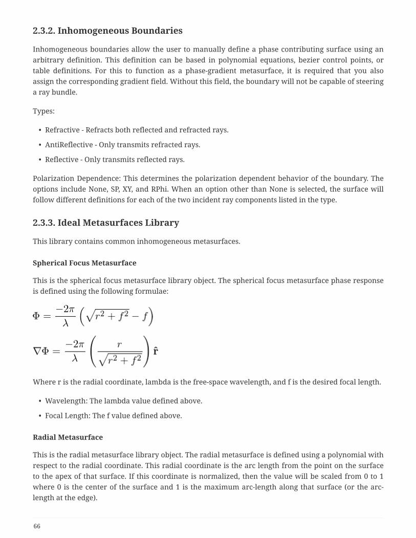
2.3.2. Inhomogeneous Boundaries

Inhomogeneous boundaries allow the user to manually define a phase contributing surface using anarbitrary definition. This definition can be based in polynomial equations, bezier control points, ortable definitions. For this to function as a phase-gradient metasurface, it is required that you alsoassign the corresponding gradient field. Without this field, the boundary will not be capable of steeringa ray bundle.

Types:

• Refractive - Refracts both reflected and refracted rays.

• AntiReflective - Only transmits refracted rays.

• Reflective - Only transmits reflected rays.

Polarization Dependence: This determines the polarization dependent behavior of the boundary. Theoptions include None, SP, XY, and RPhi. When an option other than None is selected, the surface willfollow different definitions for each of the two incident ray components listed in the type.

2.3.3. Ideal Metasurfaces Library

This library contains common inhomogeneous metasurfaces.

Spherical Focus Metasurface

This is the spherical focus metasurface library object. The spherical focus metasurface phase responseis defined using the following formulae:

Where r is the radial coordinate, lambda is the free-space wavelength, and f is the desired focal length.

• Wavelength: The lambda value defined above.

• Focal Length: The f value defined above.

Radial Metasurface

This is the radial metasurface library object. The radial metasurface is defined using a polynomial withrespect to the radial coordinate. This radial coordinate is the arc length from the point on the surfaceto the apex of that surface. If this coordinate is normalized, then the value will be scaled from 0 to 1where 0 is the center of the surface and 1 is the maximum arc-length along that surface (or the arc-length at the edge).

66

This pre-made radial metasurface contains the following properties:

• Units Choice: This allows the specification of units the radial coordinate.

• Constant Term (C0): This is the constant contribution to the phase polynomial

• Quadratic Term (C1): This is the quadratic (second order) contribution from the radial coordinate tothe polynomial.

• Quartic Term (C2): This is the quartic (fourth order) contribution from the radial coordinate to thepolynomial.

• Sextic Term (C3): This is the sextic (sixth order) contribution from the radial coordinate to thepolynomial.

Elliptic Metasurface

This is the elliptic metasurface library object. The elliptic metasurface is defined using a polynomialwith respect to the x and y Cartesian coordinates. These Cartesian coordinates are the cosine and sineof arc length from the point on the surface to the apex of that surface, then projected into a flat plane.If these coordinates are normalized, then the value will be scaled from -1 to 1 where 0 is the center ofthe surface.

This pre-made elliptic metasurface contains the following properties:

• Units Choice: This allows the specification of units the x and y coordinates.


• Quadratic X Term (C1): This is the quadratic (second order) contribution from the x coordinate tothe polynomial.

• Quartic X Term (C2): This is the quartic (fourth order) contribution from the x coordinate to thepolynomial.

• Sextic X Term (C3): This is the sextic (sixth order) contribution from the x coordinate to thepolynomial.

• Quadratic Y Term (C4): This is the quadratic (second order) contribution from the y coordinate tothe polynomial.

• Quartic Y Term (C5): This is the quartic (fourth order) contribution from the y coordinate to thepolynomial.

• Sextic Y Term (C6): This is the sextic (sixth order) contribution from the y coordinate to thepolynomial.

2.3.4. Angle Dependent Metasurfaces Library

This library contains common inhomogeneous metasurfaces.

67

Theta Dependent Radial Metasurface

This is the theta dependent metasurface library object. The theta dependent radial metasurface isfunctionally the Radial Metasurface but with terms that can be polynomially scaled with incidentangle.

The theta dependent radial metasurface is defined using the following terms:

• Units Choice: This allows the specification of units the r coordinates.


• Quadratic r Term (C1): This is the quadratic (second order) contribution from the radial coordinateto the polynomial.

• Quartic r Term (C2): This is the quartic (fourth order) contribution from the radial coordinate to thepolynomial.

• Sextic r Term (C3): This is the sextic (sixth order) contribution from the radial coordinate to thepolynomial.

• Linear r Theta Term (C4): This is the linear (first order) contribution from the incident angle scalinglinearly with the radial coordinate.

• Linear r Quadratic Theta Term (C5): This is the quadratic (second order) contribution from theincident angle scaling linearly with the radial coordinate.

2.4. ElementsLenses, prisms, mirrors, and all other geometry are modeled as Elements objects. Elements can bespecified in several ways, such as by specifying an explicit list of bounding surfaces, importing a pre-configured optic from a library, or requesting a Paraxial lens or other ideal or nonphysical element.Apertures and stops are also specified as elements. Users familiar with spreadsheet-style surface entrywill find the Lens Stack elements to be the most intuitive form of geometry entry; this is therecommended method for modeling lens geometry.

2.4.1. Lens Stacks

Lens stacks are a form of sequential surface entry, where surfaces and the materials between them arelisted in order in a table. Any sections with a non-background material (see Spatial DomainBackground Material) will be enclosed to form a lens, with the surfaces on either side forming thefront and back surfaces of the lens.

Lens Stack Editor

The Surfaces table in the lens stack property editor displays the basic properties of each surface, with arow for each surface in the stack. To add a new surface to the lens stack, click the "Add" button belowthe Surfaces table. New surfaces will be added to the end of the lens stack, but before any ImagePlanes. To remove or reposition an existing surface, click on the row corresponding to the surface and

68

click "Delete", "Move Up", or "Move Down." To view the complete list of properties for a surface, clickon the row for the surface and click the "Edit" button.

If a surface’s property is set to a parameter, editing that value in the Surfaces table will edit theparameter’s value, rather than changing the surface property directly. For instance, if a surface radiusis set to the parameter "myRadius", editing that surface in the table will change the "myRadius"parameter and leave the surface still set to myRadius. This will also occur if the surface’s property is setto a simple supported expression, such as convertCurvature(myCurvature). In this case, the Surfacestable will set the "myCurvature" parameter to the corresponding curvature for the entered radius,instead of directly changing the surface radius to the entered value. But this will not happen for morecomplex or multi-parameter expressions like myRadius + (factorValue * 2mm).

This feature is designed to make it easier to edit lens dimensions after running the OptimizationWizard, which parameterizes the lens system when it configures the optimization. However, it canlead to unexpected edits if custom parameters are used in the lens stack. Care should be taken whenusing custom parameters that the lens stack Surfaces table is editing the correct values. If this behavioris interfering with your use of parameters, you can bypass it by editing the surface properties directlywith the "Edit" button.

Lens Stack Properties

Override Color

By default, lenses in the lens stack will be rendered in the 3D modelview using the colors of theirassigned materials. If this property is checked, then Color and Transparency are used instead torender all lenses in the lens stack.

Color

The color used to render lenses in the 3D modelview, if Override Color is checked.

Transparency

The transparency used to render lenses in the 3D modelview, if Override Color is checked.

Trace Order

When Sequential Raytracing is enabled, this property determines the order in which separate lensstacks will be traced. This ordering is also used when finding the aperture stop and when solvinglens diameters.

Origin

Defines the origin point of the lens stack. This location will be the origin point of the first surface inthe stack. See the position vector documentation for explanations of the different ways the locationcan be specified.

Optical Axis

The direction in which surfaces will be added to the lens. The "back" of the lens stack is in thisdirection. See the orientation vector documentation for explanations of the different ways the

69

orientation can be specified.

Max Surface Diameter

The maximum surface diameter that will be used while solving for diameters (see Lens StackSurface Diameter).

2.4.2. Lens Stack Surfaces

Surfaces added to a lens stack define the front and back boundaries of the lenses in the stack. The mostbasic lens stack surface is the Surface type, which is a simple spherical cap defined by a radius ofcurvature.

Hide Dummy Surface

If a surface is in mid-air (surrounded by the Spatial Domain’s Background Material), this propertydetermines whether or not the surface is shown in the modelview.

Type

The type of surface to be inserted in the lens stack.

• Surface: A spherical cap with a radius of curvature. This is the most basic type of surface.

• Stop: A surface with a stop centered around the apex of curvature.

• Image Plane: A surface that can be used to determine the location of the focal plane, if the ImagePlane focus method is used.

• Asphere: An aspheric surface.

Material

The material following this surface in the lens stack. If this material is the same as the SpatialDomain’s Background Material, then there will be no lens after this surface. The last surface in alens stack must be assigned the background material.

Boundary

The boundary condition or metasurface coating applied to this surface in the lens stack.

Thickness

The distance between the apex points of this surface and the next. If this surface is assigned a non-background material (see Material), this thickness will be the thickness of the lens componentfollowing this surface.

Surface Radius

The radius of curvature of this surface. A positive radius curves the edges of the surface towards theback of the lens stack (in the same direction as the Lens Stack Optical Axis), and a negative radiuscurves the edges towards the front.

70

Diameter

The clear aperture diameter of this surface. Lens diameters are the largest of the diameters of thefront and back surfaces. For Stops, this also determines the diameter of the stop. If the diameter iszero, then the diameter will be automatically determined based on the point at which rays intersectthe surface.

Clear Aperture Margin

Provides a buffer zone at the edge of a lens. The actual lens diameter will be the sum of theDiameter and the Clear Aperture Margin.

Component Decenter

Moves a component from its default position in the lens stack by the specified position vector. Thesurface for which this is specified must be either the first surface in the lens stack or be preceded bythe Spatial Domain’s Background Material. The position of subsequent surfaces will be determinedbased on the decentered position of this surface, until after the next surface which is followed bythe background material. This value is applied before the Component Tilt.

Component Tilt

Tilts a component away from the lens stack’s Optical Axis by the specified orientation vector, withthe tilt being applied at the vertex of the surface. Note that if an absolute orientation is specifiedinstead of a tilt, it is applied not in global coordinates but relative to the lens stack orientation, so(0,0,1) would be no tilt at all regardless of the orientation of the optical axis. Subsequent surfaceswill follow the same tilted orientation, until after the next surface which is followed by thebackground material. This value is applied after the Component Decenter and has the samerestrictions as to what surfaces it can be specified for.

Lens Stack Stops

Stop surfaces are much like normal surfaces, except that in addition to the surface, a stop is centeredaround the apex of curvature, which can be used to define the simulation aperture.

Aperture Stop

If checked, this stop’s diameter is used to define the simulation’s aperture diameter, which can alsoinfluence the diameter of the source in some cases (see Beam Source properties). If no stops havethis property checked, the first one in the lens stack is used to define the aperture.

Lens Stack Image Plane

Image Plane surfaces are much like normal surfaces, but they can be used to determine the location ofthe focal plane if the Image Plane focus method is used. If this method is used, there should be only oneImage Plane surface in the simulation.

Lens Stack Aspheres

Aspheres in the lens stack are much like normal surfaces, except instead of being defined by a radius

71

of curvature alone, the sag of an aspheric surface is defined by the following equation (where R is theradius of curvature):

Conic Constant Kappa

The conic constant term in the asphere surface equation (K).

Polynomial Coefficients

The list of alpha coefficients in the asphere surface equation. The first coefficient in the list is a2 (theradius-squared term), followed by the a4 coefficient, and so on in even powers of the radius-coordinate.

Polynomial Units

The unit of length used for the radius-coordinate in the asphere surface equation. Most tools usemillimeters.

2.4.3. Bounded Elements

Bounded Elements are defined by an explicit list of bounding surfaces, such as spherical caps,aspheres, cylinders, and circles.

A ray enters an element when it collides with a surface belonging to that element, and exits theelement when it collides with a second element. By this definition, a bounded element does not requirea strict closed surface. However, modeling a geometry with open boundaries may result in rays thatmiss the second surface of an element and are not accurately refracted. This result is especiallycommon when tracing GRIN regions, which means that closed boundaries must be specified whentracing a GRIN optic.

Bounded Element Properties

Name


Override Color

Allows the user to override a material’s color and specify a lens specific color.

Surfaces

See Elements - Surfaces.

Dimensions

See Element Properties.

72

Material

Material inside the element. If the referenced material is dispersive, then the resulting optic willdemonstrate different behavior for different wavelengths. If the referenced material has a spatial(x,y,z or r,phi,z) dependence, then rays within the element will be traced using the GRIN engine.

Origin


Normal Vector


Component Temperature

Temperature of the lens. Used when computing refractive index data for materials that incorporatetemperature information.

2.4.4. Bounded Element Surfaces

Two surfaces may not be coincident; a bonded doublet or triplet lens must either use a "reference"surface to use a surface belonging to an existing lens, or a small air gap must be introduced betweenthe two sublenses.

Surfaces in reTORT belong to exactly two elements. The second element is either the implicitbackground material, or a element with an explicit "reference" surface defined.

Individual surfaces are defined with their geometric properties as well as optical surface properties(perfect Anti-reflective (AR), perfectly absorbing (ABS), perfectly reflective (PEC), or normal (NONE)).Additional boundary conditions (including real AR and partially-reflective coatings and properhandling of surface roughness) will be added in the future.

Annular Ring

An Annular Ring is the planar surface between an inner and outer circle, defined by an inner andouter diameter. Rays do not interact with this surface inside the inner circle, or outside the outer circle.

Annular rings with an absorbing (ABS) boundary condition are used to model circular stops, and slots.In absorbing mode, rays contacting the surface are terminated, and do not generate reflected orrefracted rays.

Annular Ring Properties


• Base Position - See Surface Properties.

• Normal Vector - See Surface Properties.

• Diameter - See Surface Properties.

• Inner Diameter - See Surface Properties.

73

• Boundary - See Surface Properties.

Asphere

Aspheric profiles are used to correct spherical and higher-order aberration. reTORT aspheres aredefined as cylindrically-symmetric surfaces extending from an inner to an outer diameter according tothe following equation:

In the equation, R is the effective spherical radius, kappa is the conic constant, the alpha terms are thepolynomial coefficients, r is the cylindrical radial coordinate and z is the cylindrical axial coordinate.The local cylindrical coordinate system is defined by the origin and orientation of the surface; theorientation vector defines the z-axis and uniquely defines the r-phi plane.

It is computationally inefficient to use an asphere with extremely large radius of curvature to model aflat surface; use a circle (or even a sphere with a large radius of curvature) instead.

Asphere Properties






• Surface Radius - See Surface Properties.

• Conic Constant Kappa - kappa

Specify the base shape of the aspheric surface.

kappa Conic Section

kappa < -1 hyperbola

kappa = -1 parabola

-1 < kappa < 0 ellipse (prolate spheroid)

kappa = 0 sphere

kappa > 0 ellipse (oblate spheroid)

• Polynomial Coeffs : Polynomial perturbational terms of the asphere. No scaling factors are appliedby default.


74

Circle

Planar circle defined by a radius, position, and orientation vector. Used for plano-convex lenses

Circle Properties






Cylinder

Cylindrical shell that is open at the two planar ends; only the side walls interact with rays. Cylindersare used to connect other surfaces.

Cylinder Properties





• Height - Cylinder height.


Group

Represents a collection of surfaces grouped together. A group of surfaces can be used as an importobject to allow loading multiple surfaces at a time from a library.

Group Properties


• Surfaces - See Bounded Elements.

• Origin - See Object Properties.


Reference

Surfaces may not be coincident, so any two elements that would naturally make contact over a finitearea must be defined such that one references a surface defined by the other. Bonded doublet or tripletlenses will require this approach.

75

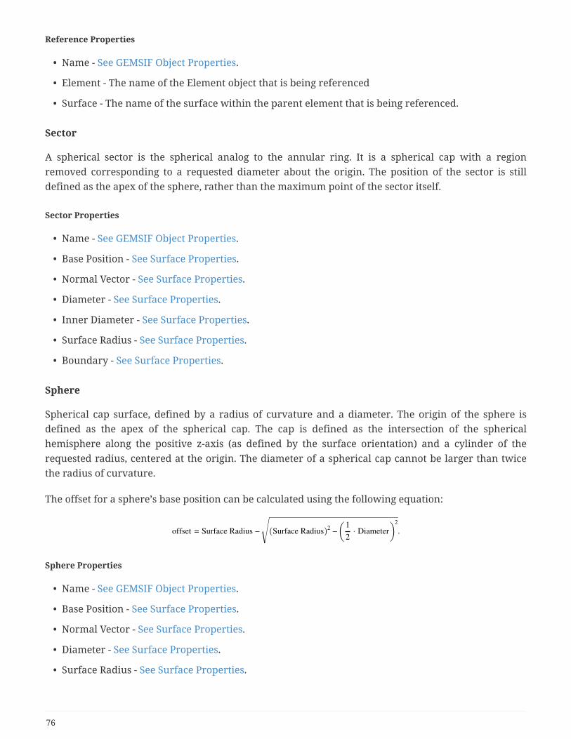
Reference Properties


• Element - The name of the Element object that is being referenced

• Surface - The name of the surface within the parent element that is being referenced.

Sector

A spherical sector is the spherical analog to the annular ring. It is a spherical cap with a regionremoved corresponding to a requested diameter about the origin. The position of the sector is stilldefined as the apex of the sphere, rather than the maximum point of the sector itself.

Sector Properties








Sphere

Spherical cap surface, defined by a radius of curvature and a diameter. The origin of the sphere isdefined as the apex of the spherical cap. The cap is defined as the intersection of the sphericalhemisphere along the positive z-axis (as defined by the surface orientation) and a cylinder of therequested radius, centered at the origin. The diameter of a spherical cap cannot be larger than twicethe radius of curvature.

The offset for a sphere’s base position can be calculated using the following equation:

Sphere Properties






76


Common Bounded Element Surface Properties

Base Position

Position of the surface relative to the owning element’s local coordinate system. See the positionvector documentation for explanations of the different ways the position can be specified.

Normal Vector

Orientation of the surface relative to the owning element’s local coordinate system. See theorientation vector documentation for explanations of the different ways the orientation can bespecified.

Diameter

Diameter of the surface normal to the local z-axis.

Inner Diameter

Inner diameter of a ring, section, or asphere normal to the local z-axis.

Surface Radius

Defines the radius of curvature for Spheres, Sectors, and Aspheres.

Boundary

Defines whether a surface is treated as Anti-Reflective (AR), Perfectly absorbing (ABS), Perfectlyreflecting (PEC), or normal (NONE).

2.4.5. Paraxial Lens

The paraxial lens represents an ideal collimating element, specified by an infinitesimally thin circularsurface and a focal length. By definition, all rays incident on the surface with the same incident angleare refracted to a point on the focal plane, and rays passing through the geometric center of theparaxial lens (specified by the origin property) are not refracted.

Paraxial Lens Properties

Name


Origin

See Object Properties - Origin.

Normal Vector


77

Diameter

Diameter of the paraxial lens.

Focal Length

Focal Length of the paraxial lens. A collimated beam incident to one side of the lens will be focusedto a point on the plane placed a focal length away from the paraxial lens along the lens’s orientationvector.

2.4.6. Stops

Stop elements can be used to define apertures in a simulation.

Stop Properties

Name


Dimensions


Color

See GEMSIF Properties

Transparency

See GEMSIF Properties

Origin


Normal Vector


Diameter

Sets the diameter of the stop.

Aperture

If checked, this stop is used to define the aperture size of the simulation.

2.4.7. Common Element Properties

Dimensions

Stores the dimension lines used on the 2D diagram.

78

Normal Vector

Orientation of the lens relative to the global coordinate system.

The local coordinate system is defined by rotating the z-axis of the global Cartesian coordinate systemto be aligned with the orientation vector. The same rotation is applied to the y- and x-axes to obtain thelocal rotated coordinate system. No control is provided at present over the local orientation or offset ofthe y- and x-axes.

See the orientation vector documentation for explanations of the different ways this vector can bespecified.

2.5. ResultsResult objects specify the calculated outputs of the simulation engine. Multiple results may be added torequest outputs computed with different inputs or parameters.

2.5.1. Ray Result

Specifies the fundamental reTORT ray data output. Additional outputs may be requested by adding"Outputs" children to the ray result.

RayResult Properties

Name


Enabled

When enabled, this result is re-evaluated when "Run All Results" is invoked on the simulation.

Generate Ray Diagram

Request generation of the ray diagram output from the ray tracer. If enabled, the rays will bedisplayed on the 3D model display.

Disable All Overlap Detection

Disables all checks for overlapping elements in the model and overlapping surfaces within lensstacks. Other validation checks are unaffected.

2.6. Ray Result Outputs

2.6.1. Optical Output

Compute outputs for imaging metrics at a requested focal plane.

Note that most results are computed relative to a focal point for each raybundle (that is, for each

79

wavelength and incident angle), where the focal point is determined by the Focus Calculation Method.Most focus calculation methods determine the lateral focal point position using the intersection of thechief ray with the focal plane. The chief ray is the ray in the center of each raybundle. If the chief raydoes not intersect the focal plane, then the first ray to intersect the focal plane will be used instead (theray with the lowest Ray ID).


• Focus Calculation Method - This option determines how the focal plane location is determined.

◦ Paraxial - The focal point is located at the intersection point of the paraxial rays in each bundle.

◦ Marginal - The focal point is located at the intersection point of the marginal rays in eachbundle.

◦ Minimum RMS - The focal plane is located at the minimum RMS spot for all rays in each bundle.The lateral focal point position is determined by the intersection of the chief ray.

◦ Minimum Peak - The focal plane is located at the minimum peak spot for all rays in eachbundle. The lateral focal point position is determined by the intersection of the chief ray.

◦ Image Plane - The focal plane is located at the Image Plane surface. The lateral focal pointposition is determined by the intersection of the chief ray.

◦ Lens Stack Surface - The focal plane is located at the surface specified by the Lens Stack andLens Stack Index properties. The lateral focal point position is determined by the intersection ofthe chief ray.

◦ Manual - The focal plane is located at the point specified by the Focal Plane property. The lateralfocal point position is determined by the intersection of the chief ray.

◦ BFL - The focal plane is located a certain distance away from the back surface of the systemalong the Optical Axis, where the distance is specified by the Target Focal Length property. Thiscan be used to target a certain back focal length during an optimization. The lateral focal pointposition is determined by the intersection of the chief ray.

◦ EFL - The focal plane is located a certain distance away from the back principal point of thesystem along the Optical Axis, where the distance is specified by the Target Focal Lengthproperty. This can be used to target a certain effective focal length during an optimization. Thelateral focal point position is determined by the intersection of the chief ray.

• Focal Plane - Manually-specified location of the focal plane, when the Focus Calculation Method isset to Manual. If set to Image Plane or Lens Stack Surface, this property will be the location of thespecified surface. Otherwise, this property will be the focal point of the first raybundle. See theposition vector documentation for explanations of the different ways the location can be specified.

• Target Focal Length - Sets the desired back focal length or effective focal length at whichmeasurements will be performed. This is used when the Focus Calculation Method is set to BFL orEFL.

• Focal Plane Diameter - Sets the effective diameter of the focal plane for the purpose of determiningwhich rays intersect it. This is used when the Focus Calculation Method is anything other thanImage Plane or Lens Stack Surface.

80

• Lens Stack - If the Focus Calculation Method is set to Lens Stack Surface, this property is used tospecify which lens stack contains the surface in question.

• Lens Stack Index - If the Focus Calculation Method is set to Lens Stack Surface, this propertyspecifies the index of the surface in question.

• Optical Axis - Sets the direction of the optical axis for the system, along which calculations arebased. See the orientation vector documentation for explanations of the different ways the axisdirection can be specified.

• Independent Group Focal Planes - This option forces each focal plane to be evaluatedindependently for each ray group.

Focal Plane Metrics

• Compute Spot Metrics - Request calculation of the spot metrics. This includes information such asfocal point location.

• Generate Spot Diagram - Request calculation of the planar spot diagram.

• Use Centroids For Spot Size Calculation - If this is checked, the centroid of each ray bundle will betreated as the average of each ray’s intersection with the focal plane, instead of where the chief rayintersects the plane. This will affect the RadialTRA result used for DLS spot size optimization, butwill not affect the focal points or spot sizes given in the FocalPoint table.

• Enable Lateral Color Correction - This is only available if "Use Centroids For Spot Size Calculation"is selected. Lateral color correction means that all ray bundles at a given incident angle - regardlessof wavelength - will be combined to determine a "joint" centroid.

Imaging Metrics

• Compute Pupil Function - Request generation of the Pupil Function.

• Compute Wavefront Error - Request generation of the OPD or Wavefront Error.

• Compute OTF - Request generation of the complex Optical Transfer Function.

• Compute MTF - Request generation of the Modulation Transfer Function image.

• Compute MTF Trace - Request generation of an MTF trace for plotting.

• Compute Zernike Coefficients* - Request Zernike Polynomial Decomposition of the WavefrontError.

• Zernike Polynomial Max Order* - Set the maximum order of Zernike Polynomial used in thedecomposition. A hard limit has been emplaced at tenth order.

• Generate Zernike Recomposition* - Request generation of a recomposed wavefront error based onthe Zernike Decomposition of the wavefront. Generally used to smooth over noisy data.

• Use Zernike Recomposition* - Request that the Zernike Recomposed wavefront error be used inplace of the normally generated OPD.

• Compute Seidel Coefficients* - Request generation of the Seidel Aberration Coefficients for the

81

given Wavefront Error. These coefficients are approximated through combination of appropriateZernike Polynomial Coefficients.

• Compute RMS Wavefront Error - Request Calculation of the RMS value of the Wavefront Error.

• Compute Point Spread Function - Request generation of the Point Spread Function.

Ray Aberration Curves

• Compute Transverse Ray Aberration - Request a 2D plot of the Transverse Ray Aberration acrossthe pupil.

• Compute Meridonal TRA - Request a trace of the Transverse Ray Aberration across the MeridonalPlane of the pupil.

• Compute Sagittal TRA - Request a trace of the Transverse Ray Aberration across the Sagittal Plane ofthe pupil.

• Compute Longitudinal Ray Aberration - Request a 2D plot of the Longitudinal Ray Aberrationacross the pupil.

• Compute Meridonal LRA - Request a trace of the Longitudinal Ray Aberration across the MeridonalPlane of the pupil.

• Compute Sagittal LRA - Request a trace of the Longitudinal Ray Aberration across the Sagittal Planeof the pupil.

Results with an asterisk (*) are advanced properties made visible through the "Toggle AdvancedProperties Visibility" button indicated by the pair of gears ( ) in the property editor.

2.6.2. Paraxial Output

This output contains paraxial information about the system including EFL, BFL, Entrance and ExitPupil information and similar information. For more detail see the Paraxial System Data Tabledocumentation.

Paraxial System Data Result Table

This output contains the following information on a Per Wavelength basis:

• System Back: The distance from the source along the optical axis to the physical back point of thesystem.

• Front Principal Point: The distance from the source along the optical axis to the front principalpoint or nodal point of the system.

• Back Principal Point: The distance from the source along the optical axis to the back principal pointor nodal point of the system.

• Front Focal Point: The distance from the source along the optical axis to the front paraxial focalpoint.

• Back Focal Point: The distance from the source along the optical axis to the back paraxial focal

82

point.

• Effective Focal Length: The distance from the Back Principal Point along the optical axis to the BackFocal Point.

• Back Focal Length: The distance from the System Back along the optical axis to the Back Focal Point.

• Entrance Pupil Location: The distance from the source along the optical axis to the center of theEntrance Pupil.

• Entrance Pupil Size: The diameter of the Entrance pupil.

• Exit Pupil Location: The distance from the source along the optical axis to the center of the ExitPupil.

• Exit Pupil Size: The diameter of the Exit pupil.

2.7. Common reTORT Object Properties

2.7.1. Origin

Specify the location of the object relative to the parent or global coordinate system. See the positionvector documentation for explanations of the different ways the location can be specified.

2.7.2. Orientation

Specify the orientation of the object in terms of the global coordinate system. See the orientation vectordocumentation for explanations of the different ways the location can be specified.

3. ViewsSee also GEMSIF Views.

3.1. Model ViewDisplay a 3D rendered model of the optical system geometry and some of the output data.

3.1.1. Model View Properties

Axes Visible

Hide or show the axes in the model view.

Boundary Box Visible

Hide or show the boundary box in the model view.

83

4. WizardsSeveral reTORT wizards are provided for your convenience. These wizards can assist in setting upoptimizations and generating common plots such as spot diagrams.

4.1. Optimization WizardThis is a wizard for setting up and running optimizations. It is divided into three tabs for selectingwhat properties to optimize, what goal to optimize for, and what optimizers to use.

4.1.1. Optimizer Selection

The first time the optimization wizard is run in a given simulation, a dialog appears with a dropdownto select what types of optimizers should be initialized. Either a global CMAES optimization, a localDamped Least-Squares optimization, or both, can be initialized.

4.1.2. Parameters Tab

This tab lists commonly-optimized properties of the current simulation, and allows control over whichproperties are optimized. Radii-of-curvature properties will be optimized as curvature.

Optimized Checkbox

If checked, the parameter for this row will be optimized.

Parameter Name

The name of the parameter for this row. Material and boundary coefficients are listed as thematerial/boundary name followed by the property name. Lens stack properties are listed by thename of the lens stack, followed by the number of the surface in the stack, followed by the propertyname.

Current Value

Current value of the parameter. For radii-of-curvature properties, this value is the currentcurvature.

Min Value

Minimum value of the parameter during the optimization. For radii-of-curvature properties, this isthe minimum curvature.

Max Value

Maximum value of the parameter during the optimization. For radii-of-curvature properties, this isthe maximum curvature.

Enforce Global Bounds

If checked, the global CMAES optimization will not allow properties to stray beyond their specified

84

Min Value and Max Value. See CMAES - Respect Bounds.

Enforce Local Bounds

If checked, the local DLS optimization will not allow properties to stray beyond the specified MinValue and Max Value. See DLS - Respect Bounds.

Advanced Parameter Settings

This dialog lists more advanced parameter settings, such as parameter pickups.

Type

Defines the parameter type:

• Fixed - The parameter is set directly by the user, and will not be optimized.

• Optimized - The parameter is set directly by the user, and will be optimized when either of theRun Optimization buttons are pressed.

• Pickup - The parameter is defined by another parameter’s value, and is not set directly. Theparameter’s value is defined as , using the Reference, Factor, and Offsetproperties.

Pickup Reference

For Pickup parameters, sets the source parameter whose value will be copied. Only parameters ofthe same category as the current parameter will be listed (eg, curvatures, thicknesses, materialcoefficients).

Pickup Factor

For Pickup parameters, sets the factor by which the source parameter’s value will be multiplied.

Pickup Offset

For Pickup parameters, sets an offset that is added to the source parameter’s scaled value.

4.1.3. Goals Tab

This tab configures the metric used for the optimization goal, as well as the focal plane at which thatmetric is computed.

Focal Method

Determines the method for computing the location of the focal plane.

• Image Plane - The focal plane is positioned at the Image Plane surface.

• Back Focal Length - The Focal Length property is used to set the distance of the focal plane fromthe back of the lens system.

• Effective Focal Length - The Focal Length property is used to set the distance of the focal planefrom the second principal plane.

85

Focal Length

If the Focal Method is set to either Back Focal Length or Effective Focal Length, this determines thedistance from the focal plane to the corresponding reference point.

Use Centroid For Spot Size Calculation

If this is checked, the centroid of each ray bundle will be treated as the average of each ray’sintersection with the focal plane, instead of where the chief ray intersects the plane.

Enable Lateral Color Correction

This is only available if "Use Centroid For Spot Size Calculation" is selected. Lateral color correctionmeans that all ray bundles at a given incident angle - regardless of wavelength - will be combined todetermine a "joint" centroid.

Primary Goal

Sets the metric used for optimization. Optimizations can minimize either spot size or RMSwavefront error.

Secondary Goals

Lens Center Thickness

Minimum and maximum allowable values for the center thickness of individual lenses in thelens stack. Optimizations may consider either, both, or neither.

Lens Edge Thickness

Minimum and maximum allowable values for the edge thickness of individual lenses in the lensstack. Optimizations may consider either, both, or neither.

Airgap Center Thickness

Minimum and maximum allowable values for the center thickness of individual airgaps in thelens stack. Optimizations may consider either, both, or neither.

4.1.4. Optimizer Settings Tab

This tab defines which optimizers are configured by the wizard, and the optimizer-specific settingsused for each type.

Global Optimizer Settings

Global Optimizer Enabled

If checked, the wizard will configure a global CMAES optimization.

Global Function Limit

The maximum number of simulation runs for a single optimization run. See CMAES - FunctionCall Limit.

86

Global Generation Limit

The maximum number of CMAES generations for a single optimization run. See CMAES -Generation Limit.

Global Enforce Bounds

If checked, the optimization will not allow properties to stray beyond their Min Value and MaxValue specified in the Parameters Tab. See CMAES - Respect Bounds.

Local Optimizer Settings

Local Optimizer Enabled

If checked, the wizard will configure a local Damped Least-Squares optimization.

Local Function Limit

The maximum number of simulation runs for a single optimization run. See DLS - Function CallLimit.

Local Iteration Limit

The maximum number of CMAES iterations for a single optimization run. See DLS - IterationLimit.

Local Enforce Bounds

If checked, the optimization will not allow properties to stray beyond their Min Value and MaxValue specified in the Parameters Tab. See DLS - Respect Bounds.

4.2. Plotting WizardsSeveral plotting wizards are provided to automatically configure common plots, graphs, and diagramsof a selected focal plane, source, wavelength, and incident angle. Clicking 'OK' will create a plot withthe selected settings. Running a plotting wizard multiple times will overwrite previously-generateddiagrams from that wizard.

Optical Output

Selects the optical output whose focal plane will be used to compute the diagram/plot. If "CreateNew Output" is selected, then a new optical output will be created with the specified focal planesettings. See Optical Output.

Focus Method

Sets the Focal Calculation Method for the selected optical output.

Focal Plane

Sets the Focal Plane location for the selected optical output. This property is only displayed if theFocus Method is set to Manual. See the position vector documentation for explanations of thedifferent ways the location can be specified.

87

Focal Length

Sets the Target Focal Length of the selected optical output. This property is only displayed if theFocus Method is set to BFL or EFL.

Lens Stack

Selects the Lens Stack to be used by the selected optical output. This property is only displayed if theFocus Method is set to Lens Stack Surface.

Lens Stack Index

Sets the Lens Stack Index to be used by the selected optical output. This property is only displayed ifthe Focus Method is set to Lens Stack Surface.

Source

Selects the source whose rays will be used to generate the diagram/plot. If "All Sources" is selected,then rays from all sources will be included in the plot. See Sources.

Wavelength

Selects the wavelength to include in the diagram/plot. If "All Wavelengths" is selected, then rays ofany wavelength will be included in the plot. See Spectral Lines.

Incident Elevation Angle

Selects the incident elevation angle to include in the diagram/plot. If "All Angles" is selected, thenrays of any incident elevation angle will be included in the plot. See Incident Elevation Angle.

4.2.1. Spot Diagram Wizard

The spot diagram wizard configures a 2D spot diagram illustrating where each ray intersects theselected focal plane. See Plotting Wizards for more information.

4.2.2. Wavefront Error Plot Wizard

The wavefront error plot wizard configures a contour plot illustrating the wavefront error at theselected focal plane. See Plotting Wizards for more information.

4.2.3. MTF Graph Wizard

The MTF graph wizard configures a graph of the MTF trace at the selected focal plane. See PlottingWizards for more information.

Trace Axis

Selects whether the meridonal MTF, sagittal MTF, or both are plotted.

4.2.4. TRA Trace Wizard

The TRA trace wizard configures a graph of the TRA trace at the selected focal plane. See Plotting

88

Wizards for more information.

Trace Axis

Selects whether the meridonal TRA, sagittal TRA, or both are plotted.

4.3. Save Wavefront Profile WizardThe Save Wavefront Profile wizard saves the current wavefront profile at the selected focal plane foruse in later wavefront-matching optimizations. See Plotting Wizards for more information.

See also Clear Wavefront Profiles Wizard.

Name

The name under which to save the wavefront profile.

4.4. Clear Wavefront Profiles WizardThis wizard deletes any wavefront profiles that have been saved by the Save Wavefront ProfileWizard, and disables any wavefront-matching results that used those profiles.

89

Topical Documentation for PFSS

1. PFSS SimulationPFSS models the electromagnetic response of a periodic tiling of rectangular multilayered metallo-dielectric unit cells to an incident plane wave. The PFSS Simulation plugin provides the additionalcapabilities to GEMSIF to design, build, and simulate periodic tiling of unit cells. Two solvers arecontained in the plugin, PFEBI and PMM. Details…

1.1. Objects and Collections• Actions

• Parameters

• Boundary Conditions

• Materials

• Spatial Domain

• Excitations

• Layers

• Patterns

• Results

• Views

• Layer Dock

• Stackup View

1.2. DetailsA simulation is defined and constructed by the objects contained within it. The objects can be brokeninto three categories: general simulation characteristics, component properties, and layers. Generalsimulation properties contain the physical dimensions of the simulation and consist of a SpatialDomain object and one or more excitation objects. Component properties define the building blocks ofthe simulation. These consist of Boundary Conditions, Materials, and Pattern objects. Finally, Layersconsist of the Layer object which reference the component property objects to build the simulation. Asimulation must have at least one material or boundary condition layer.

1.3. See Also• Introduction to PFSS

90

• PFSS Simulation Model

• PFSS Solvers

2. Objects and Properties

2.1. Spatial DomainOnly one Spatial Domain object is permitted for each PFSS simulation. The spatial domain objectsspecifies the physical dimensions of the unit cell and mesh properties used by the solver.

2.1.1. Spatial Domain Properties

Name


Bottom Deembed Distance

Specifies the phase deembedding distance to be applied to the bottom surface of the unit cell. Thebottom deembedding distance affects both the reflection and transmission phase values.

Property: Length, default value "0 cm".

NOTESee the deembed explanation in Top Deembed Distance for an explanation of thedeembed property.

Top Deembed Distance

Specify the phase deembedding distance to be applied to the top surface of the unit cell. The topdeembedding distance affects both the reflection and transmission phase values.


When designing for a specific reflection or transmission phase profile, often the designer will have aspecific phase reference plane that may not correspond to the top layer of the simulation domain. Thisfactor is relevant in the design of high-impedance surfaces (Sievenpiper surfaces, or Artificial MagneticConductors) or reflectarray unit cells. Setting the deembed distance moves the phase reference planeinwards into the topmost (bottommost) layer of the simulation. Deembedding will only consider thematerial parameters of the topmost (bottommost) layer even if the deembeding thickness is greaterthan the top (bottom) layer thickness.

Height

Specify the size of the unit cell along the y-axis.

91

Property: Length, default value "1 m".

NOTEPlease see width for constraints and considerations on the unit cell and pixeldimensions.

Max Voxel Aspect Ratio

Specify the maximum aspect ratio (layer thickness / max (pixel width, pixel height)) of the voxels infinite-thickness material layers. Set to zero to disable automatic layer subdivision.

Property: Positive double quantity.

NOTE This property is used only by the PFEBI solver and ignored by the PMM solver.

When modeling layers of finite-thickness dielectric in PFEBI, the layer as specified in the simulationconfiguration must be split into thinner layers for use by the solver. The solver prefers the voxels(whose dimensions are determined by the layer thickness and the domain properties width, height, nX,and nY) to be nearly cubical (aspect ratio of 1.) However, for very thick layers, this constraint canresult in extremely long simulation times. Increasing the maximum aspect ratio generates fewersimulation layers, reducing the simulation complexity and computational time. Using excessively largevoxel aspect ratios may reduce the accuracy of the PFEBI solver.

IMPORTANTIf the Max Voxel Aspect Ratio is set to zero, then material layers will not beautomatically remeshed into thin layers by the solver, and the calculated resultsmay be inaccurate.

Pixels, X

Specify the number of pixels in the unit cell along the x-axis.

Property: Positive, nonzero integer quantity.

The number of pixels in the simulation is used by the solvers as the simulation mesh. The effectivenumber of pixels in the simulation The number of pixels in the domain should be specified accordingto the geometrical or fabrication constraints of the design, with increased meshing for simulations athigh frequencies specified by an oversampling factor in the relevant Excitation objects.

NOTEPlease see width for constraints and considerations on the pixel count and dimensionswithin the simulation.

Pixels, Y

Specify the number of pixels in the unit cell along the y-axis.

Property: Positive, nonzero integer quantity.

92

NOTEPlease see width for constraints and considerations on the pixel count and dimensionswithin the simulation.

Constraint

See Object Properties - Pattern Constraint

Width

Specify the size of the unit cell along the x-axis.

Property: Length, default value "1 m".

The PFSS solvers are sensitive to the physical size of the unit cell. The formulations of the solvers werederived with the assumption that the unit cell lateral dimensions are each less than a wavelength inthe dielectric material; therefore, the highest accuracy and simulation speed is achieved whenmodeling periodic structures whose unit cells are smaller than a wavelength. In practice, theconstraint is often reduced to require that the unit cell dimensions be less than one wavelength in freespace. Violating this soft constraint will increase the number of solver iterations required to convergeto a solution, and may decrease solver accuracy, especially the PMM solver.

The unit cell width (or height) and the number of pixels along the x axis (or y axis) should be selectedsuch that the maximum pixel width (width/nX) is less than λ/10 at the highest simulation frequencywithin the material with the highest index in the simulation (see the PMM and PFEBI solver limitationsfor more details). Alternatively, nX may be set to a logical size to satisfy the geometric constraints onthe design problem and use the oversample property of the excitation object to a sufficiently largevalue to satisfy the maximum pixel size constraints.

2.2. ExcitationsExcitations specify the frequency and angular sweep settings of the incident field used by the solver toexcite the periodic geometry defined by the layers and patterns in the simulation. One or moreexcitations must be defined to perform a simulation. All excitations may be run at once, or theindividual excitations may be selected and run to obtain only a single set of results at a time.

2.2.1. Excitation Types

• Excitation with Automatic Solver : Selects the best solver based on the simulation geometry.

• PFEBI Excitation : Creates an excitation object that uses the PFEBI Solver (flexible). Primarily usedfor modeling geometries with nonuniform dielectric layers.

• PMM Excitation : Creates an excitation object that uses the PMM Solver (faster). Primarily used formodeling geometries with homogeneous dielectric layers.

93

2.2.2. Frequency Considerations

When specifying the simulation frequency range, the electrical size of the unit cell at the upper andlower frequency points must be considered. The solvers may have stability or accuracy problems whenthe electrical size of the unit cell increases past one wavelength, and the pixel dimensions shouldremain smaller than λ/10 in both dimensions (see the PMM and PFEBI solver limitations for moredetails). In simulations over a wide frequency range, it can be worthwhile to break the simulationrange into multiple excitations so that the oversample factor may be increased for the high frequencysimulations, providing accuracy without increasing simulation time at the low frequencies.

Depending on the required simulation frequency range, the user should either specify an automaticoversampling factor or a high enough factor to satisfy the pixel size constraints.

2.2.3. Auto Solver

PFSS will automatically attempt to identify which solver to use. The Auto Solver is biased towards PMMfor improved simulation speed unless unsupported features (such as patterned material layers, orpixel dimensions that are not powers of 2) are requested in the simulation.

The Auto Solver excitation also lacks some of the more advanced simulation constraints that can be setusing a particular solver’s excitation.

Auto Solver Properties

Name


Frequency Count

See Excitation Properties - Frequency Count

Frequency Start

See Excitation Properties - Frequency Start

Frequency Step

See Excitation Properties - Frequency Step

Frequency Step Type

See Excitation Properties - Frequency Step Type

Frequency Stop

See Excitation Properties - Frequency Stop

Near Fields

See Excitation Properties - Near Fields

94

Oversample

See Excitation Properties - Oversample

Phi Start

See Excitation Properties - Phi Start

Phi Step

See Excitation Properties - Phi Step

Phi Stop

See Excitation Properties - Phi Stop

Polarization

See Excitation Properties - Polarization

Scattered Fields

See Excitation Properties - Scattered Fields

Theta Start

See Excitation Properties - Theta Start

Theta Step

See Excitation Properties - Theta Step

Theta Stop

See Excitation Properties - Theta Stop

2.2.4. PFEBI Solver

Creates an excitation object that uses the PFEBI Solver (flexible). Primarily used for modelinggeometries with nonuniform dielectric layers.

See the Solver Criteria Table for a quick reference to the best solver to use.

PFEBI Solver Properties

Name


Frequency Count


Frequency Start


95

Frequency Step


Frequency Step Type


Frequency Stop


Maximum Iterations

See Excitation Properties - Maximum Iterations

Minimum Iterations

See Excitation Properties - Minimum Iterations

Near Fields


Oversample


Phi Start


Phi Step


Phi Stop


Polarization


Scattered Fields


Theta Start


Theta Step


Theta Stop


96

Tolerance

See Excitation Properties - Tolerance

2.2.5. PMM Solver

Creates an excitation object that uses the PMM Solver (faster). Primarily used for modeling geometrieswith homogeneous dielectric layers.

See the Solver Criteria Table for a quick reference to the best solver to use.

PMM Solver Properties

Name


Frequency Count


Frequency Start


Frequency Step


Frequency Step Type


Frequency Stop


Maximum Iterations

See Excitation Properties - Maximum Iterations

Minimum Iterations

See Excitation Properties - Minimum Iterations

Near Fields


Oversample


Phi Start


97

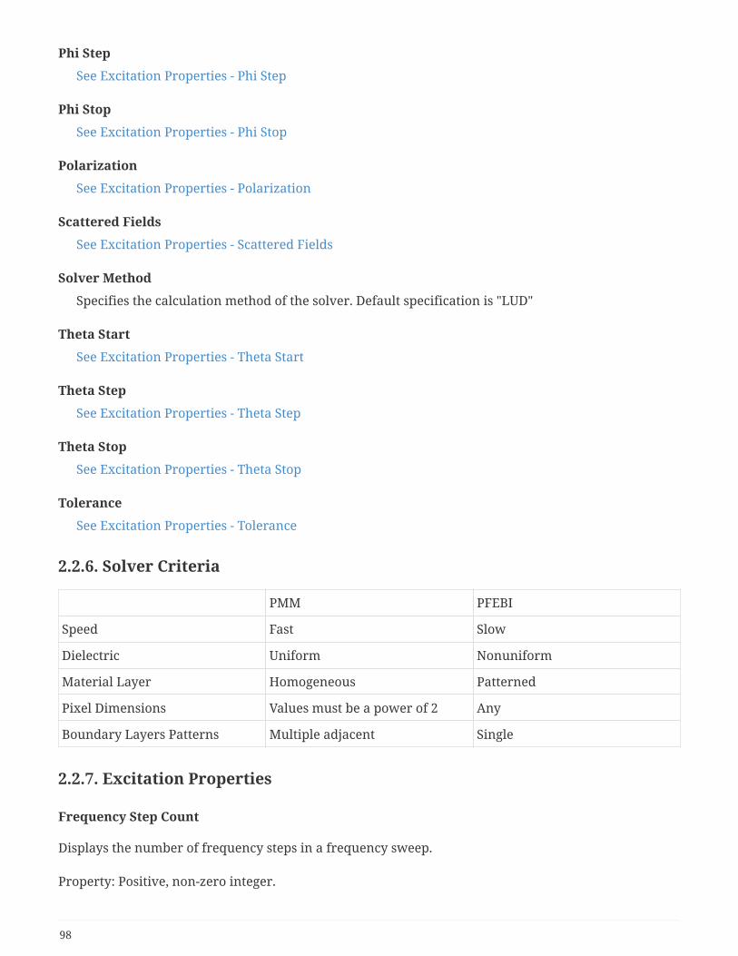
Phi Step


Phi Stop


Polarization


Scattered Fields


Solver Method

Specifies the calculation method of the solver. Default specification is "LUD"

Theta Start


Theta Step


Theta Stop


Tolerance

See Excitation Properties - Tolerance

2.2.6. Solver Criteria

PMM PFEBI

Speed Fast Slow

Dielectric Uniform Nonuniform

Material Layer Homogeneous Patterned

Pixel Dimensions Values must be a power of 2 Any

Boundary Layers Patterns Multiple adjacent Single

2.2.7. Excitation Properties

Frequency Step Count

Displays the number of frequency steps in a frequency sweep.

Property: Positive, non-zero integer.

98

NOTE frequencyStop is used when frequencyStepType is set to either Count or Logarithmic.

Frequency Start

Lower frequency limit for the frequency sweep. If Frequency Stop-Frequency Start < Frequency Step,then Frequency Start is the only frequency simulated.

Property value: Frequency, default value "1 GHz"

NOTEsee Frequency Considerations for more information on the impact of the frequencysweep range.

Frequency Step

Step size for the frequency sweep. Either Frequency Step or Frequency Step Count are required,depending on the value of Frequency Step Type.


NOTE Frequency Step is used only when Frequency Step Type is set to Linear.

Frequency Step Type

Frequency Step Type is an enumerated field that may only take on one of the following values:

Linear

Specify the start frequency, step size, and maximum allowed frequency. Note that, unless the stepsize is an exact factor of the frequency band specified by Frequency Start - Frequency Stop, thenFrequency Stop will not be included as a simulation point.

Count

Specify an exact number of frequency points to be simulated in Frequency Count in even stepsbetween Frequency Start and Frequency Stop.

Logarithmic

Specify a sweep with logarithmic spacing between frequencies Frequency Start and Frequency Stopwith exactly Frequency Count frequency points in the sweep.

The default value is Linear, which requires the properties Frequency Start, Frequency Stop, andFrequency Step to be specified. Count and Logarithmic require Frequency Start, Frequency Stop, andFrequency Count to be specified.

Frequency Stop

Upper frequency limit for the frequency sweep. If Frequency Step is specified, then the highestfrequency to be simulated is where n is the largest integer such

99

that .


NOTEsee Frequency Considerations for more information on the impact of the frequencysweep range.

Maximum Iterations

The maximum number of iterations allowed before convergence is terminated in the BCG solver. If thesolver requires more than the specified number of iterations to converge, then the convergence will beterminated early and the current results returned, with possible loss of accuracy. Reducing themaximum iteration count can decrease the worst-case simulation time, but potentially increase theprobability of simulation inaccuracies.

Positive integer, default value of 4000.

NOTE This property is only used if solverMethod is "BCG", and ignored otherwise.

Minimum Iterations

The minimum number of iterations allowed before convergence in the BCG solver. Positive integer,with a default of 3. Increasing the minimum iteration count can help to prevent preconvergence insome problems.


Near Fields

Currently not used.

Oversample

Specify the oversampling factor for the unit cell pixel counts nX and nY from the simulation domain. Ifoversample is set to zero, the program will automatically select an oversample value based on theexcitation wavelength and the unit cell and pixel dimensions specified in the domain object. A non-unity oversample value replaces each pixel in the simulation by a group of n x n pixels for the solver.For example, a simulation of an 8x8 periodic geometry with an oversample property of 3 will bemodeled with a 24x24 pixel geometry by the solver. The unit cell dimensions do not change whenmodifying oversample. Increasing the oversample factor increases the simulation mesh size in thesolver and increases the required solution time.

Both PFSS solvers use the pixel count as specified as the domain to form their simulation mesh. Thesolvers converge with higher accuracy when the pixel dimensions are small with respect to thewavelength (maximum pixel dimension should be less than lambda/10 within the dielectric material ateach simulation frequency); when this constraint is not met, the iterative solvers may produce

100

accurate results, inaccurate results, or may not converge at all.

The oversample property of the Excitation object allows the geometry of a simulation to be specified ata 1-1 scaling with the fabrication requirements, even if such pixels would be very large with respect toa wavelength. Specifying a nonunity oversample factor to increase the grid resolution when simulatingat high frequencies will help to ensure simulation accuracy.

Property value: Positive integer, default value of 1

NOTE Oversample value of 0 corresponds to "Auto" and a value of 1 corresponds to "None".

Phi Start

Specify the lower bound of the phi sweep of the incident plane wave. In general, phi may take onvalues between 0 and 360 degrees (0 and 2π rad), PMM restricts Phi Start to 1. Zero degrees is parallelwith the positive X-axis, ninety degrees is parallel to the positive Y-axis.

The phi angle of the incident wave determines the orientation of the electric field vector with respectto the X-axis, which will be different between the TE and TM incident polarizations.

Property: Angle dimensioned quantity, default value 0 or 1 deg.

Phi Step

Specify the step size of the phi sweep of the incident plane wave.

Property: Angle dimensioned quantity, default value 1 deg.

Phi Stop

Specify the upper bound of the phi sweep of the incident plane wave. If Phi Stop is less than or equal toPhi Step, then only a single incident phi angle is simulated. Phi Stop is generally limited to 360 degrees,PMM restricts Phi Stop to 359 degrees.


Polarization

Specify the polarization of the incident field. Polarization is an enumerated value that must take onone of the following values:

TE

Transverse-electric field polarization; the incident plane wave is oriented such that the electric fieldis perpendicular to the normal vector of the unit cell surface.

TM

Transverse-magnetic field polarization; the incident plane wave is oriented such that the magnetic

101

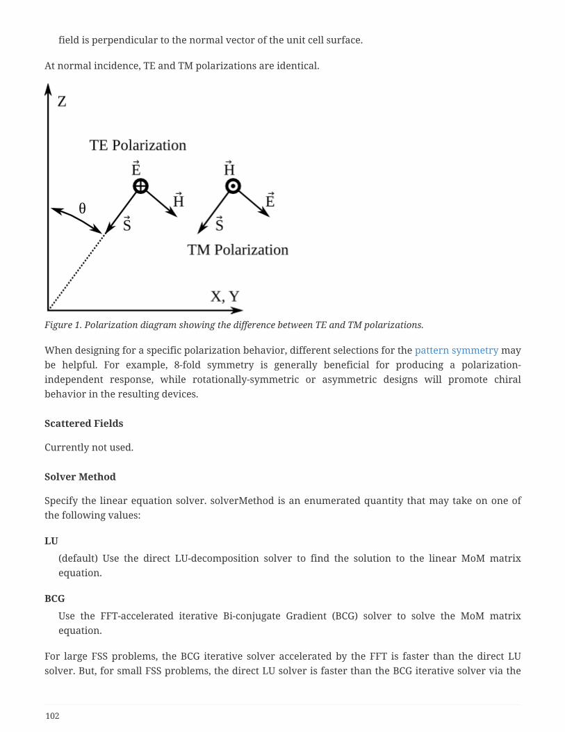
field is perpendicular to the normal vector of the unit cell surface.

At normal incidence, TE and TM polarizations are identical.

Figure 1. Polarization diagram showing the difference between TE and TM polarizations.

When designing for a specific polarization behavior, different selections for the pattern symmetry maybe helpful. For example, 8-fold symmetry is generally beneficial for producing a polarization-independent response, while rotationally-symmetric or asymmetric designs will promote chiralbehavior in the resulting devices.

Scattered Fields

Currently not used.

Solver Method

Specify the linear equation solver. solverMethod is an enumerated quantity that may take on one ofthe following values:

LU

(default) Use the direct LU-decomposition solver to find the solution to the linear MoM matrixequation.

BCG

Use the FFT-accelerated iterative Bi-conjugate Gradient (BCG) solver to solve the MoM matrixequation.

For large FSS problems, the BCG iterative solver accelerated by the FFT is faster than the direct LUsolver. But, for small FSS problems, the direct LU solver is faster than the BCG iterative solver via the

102

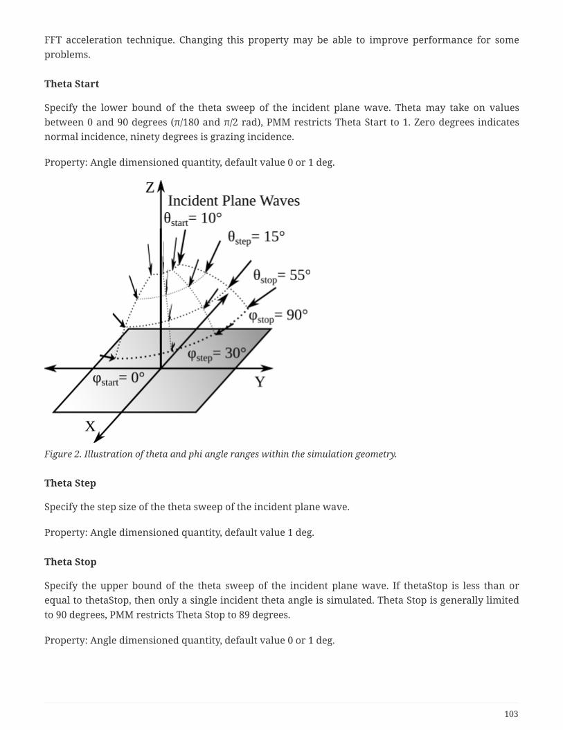
FFT acceleration technique. Changing this property may be able to improve performance for someproblems.

Theta Start

Specify the lower bound of the theta sweep of the incident plane wave. Theta may take on valuesbetween 0 and 90 degrees (π/180 and π/2 rad), PMM restricts Theta Start to 1. Zero degrees indicatesnormal incidence, ninety degrees is grazing incidence.


Figure 2. Illustration of theta and phi angle ranges within the simulation geometry.

Theta Step

Specify the step size of the theta sweep of the incident plane wave.

Property: Angle dimensioned quantity, default value 1 deg.

Theta Stop

Specify the upper bound of the theta sweep of the incident plane wave. If thetaStop is less than orequal to thetaStop, then only a single incident theta angle is simulated. Theta Stop is generally limitedto 90 degrees, PMM restricts Theta Stop to 89 degrees.


103

Tolerance

The convergence tolerance setting for the bi-conjugate gradient (BCG) iterative linear equation solver.A positive quantity less than one, 0.001 by default. Decrease the value to increase the difficulty of theconvergence condition.


2.3. Boundary ConditionsBoundary conditions represent infinitely thin layers used to specify the electromagnetic behavior ofsurfaces. Boundary conditions are used to model metallic surfaces (lossy or ideal) for RF designs, aswell as lumped elements. At optical and infrared wavelengths, it is typically more accurate to modelmetals and conductors as lossy dielectrics, rather than as a boundary layer.

2.3.1. Boundary Condition Types

• Impedance Boundary Condition : Specify a complex surface impedance value as the surfaceproperty.

• Material Boundary Condition : Specify the surface impedance based on the complex and(potentially) dispersive permittivity and permeability of an isotropic material.

• Lumped RLC Element Boundary Condition : Specify the surface impedance to be equivalent to aparallel or series combination of lumped resistance, capacitance, and inductance.

• Simple Boundary : Transparent (no boundary condition) or PEC.

2.3.2. Impedance Boundary

The impedance boundary condition specifies a nondispersive complex surface impedance. The surfaceimpedance is specified in units of ohms, and may be lossy, lossless, inductive, capacitive, or anycombination. If the impedance is small (near zero), then the impedance boundary condition should bereplaced with a PEC boundary condition.

Impedance Boundary Properties

Name


Color


Impedance

Complex surface impedance, specified as a complex number in units of ohms. If the magnitude ofthe impedance is too small, the solver will prompt the user to replace the impedance boundarycondition with a PEC boundary condition.

104

Property: Impedance, default value 0 ohms.

Transparency


2.3.3. Material Boundary

The material boundary condition specifies the complex surface impedance using a potentiallydispersive and lossy isotropic material. The effective surface impedance will be computed from thecomplex material permittivity and permeability.

The material boundary condition may be used to simulate a thin layer of lossy copper in an RFsimulation, for example. At higher frequencies, however (infrared and optical), metals and conductorsshould be specified with volumetric layers instead of a boundary condition for higher simulationaccuracy.

The specified material must not be an active (gain) medium. Any active materials specified in asimulation will generate an error.

NOTEAt present, only nondispersive material parameters are supported, and must beentered directly into the boundary condition editor. Library integration with theGEMSIF material library will be added in the future.

Material Boundary Properties

Name


Color


Epsilon

Complex relative electric permittivity of the effective material. Unitless quantity, default to 1 (freespace).

Mu

Complex relative magnetic permeability of the effective material. Unitless quantity, default to 1(free space).

Sigma

Material conductivity in units of Siemens/meter. Default value is "0 S / 1m".

Transparency


105

2.3.4. RLC Boundary

The RLC boundary condition allows the specification of the frequency-dispersive surface impedance asa combination of lumped element values (resistance, capacitance, inductance) in either a parallel orseries configuration. Each pixel of the simulation that is marked with an RLC boundary condition,regardless of the physical size of the pixel or model, will have an assigned surface impedance thatproduces the effect of the requested lumped element values.

The orientation of the lumped elements must be specified as either the X- or Y-axes. A single simulationmay only have a single x-directed and a single y-directed RLC boundary condition for seriesconnections, and one of each direction for the parallel specification as well, although the sameboundary condition may be applied to multiple pixels in the model and on multiple layers.

RLC Boundary Properties

Name


R

The resistance must be specified as a dimensioned quantity, with units of ohm, Mohm, etc. Anegative value for resistance will disable the resistor from the parallel or series combination.

L

The inductance must be specified as a dimensioned quantity, with units of H, mH, uH, etc. Anegative value for inductance will disable the inductor from the parallel or series combination.

C

The capacitance must be specified as a dimensioned quantity, with units of F, uF, nF, etc. A negativevalue for capacitance will disable the capacitor from the parallel or series combination.

Color


Direction

The specified direction of the lumped boundary condition does not affect the operation of elementin different directions, but it does affect the calculation of the effective surface impedance of thepixel in the case of non-square pixels. For rectangular pixels, the desired lumped element value isonly correct for current propagating in the specified direction. In square geometries, the directionparameter has no effect on the results.

Direction is an enumerated quantity that must take on one of the following values:

• x : The lumped element will connect the front and back faces of the pixel through the lumpedimpedance.

• y : The lumped element will connect the left and right faces of the pixel through the lumped

106

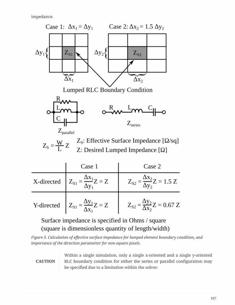
impedance.

Figure 3. Calculation of effective surface impedance for lumped element boundary condition, andimportance of the direction parametter for non-square pixels.

CAUTIONWithin a single simulation, only a single x-oriented and a single y-orientedRLC boundary condition for either the series or parallel configuration maybe specified due to a limitation within the solver.

107

Transparency


Type

Type is an enumerated quantity that must take on one of the following values:

• Series : The effective lumped impedance will be computed with a series connection of theconstituent elements.

• Parallel : The effective lumped impedance will be computed with a parallel combination of theconstituent elements.

2.3.5. Simple Boundary

The simple boundary specifies either a null boundary condition or a PEC boundary condition, based onthe value of the type property.

Simple Boundary Properties

Name


Color


Transparency


Type

Type is an enumerated quantity that must take on one of the following values:

• transparent : Specifies a transparent, or empty, boundary condition.

• pec : Specifies a perfectly-electrically conducting boundary condition.

2.4. PatternA pattern is a rectangular array or image of boolean values that may be either true or false. Each valueis associated with a pixel. When associated with a material or boundary condition in a pattern-layer,the pattern applies the specified material/boundary condition to its assigned layer at each pixel. Thepixel dimensions of the pattern may be any factor of of the simulation size specified in Domain.Patterns may be assigned a symmetry constrain that forces reflective and/or rotational symmetryalong one or both axes (x and/or y).

Patterns may be specified as a bit string that is mapped directly to the list of pixels, as a rectangularregion specified as a start and end point, or as a real-valued function of the pixel coordinates over

108

which a threshold is applied to determine the boolean state of each pixel.

2.4.1. Binary Pattern

A binary pattern uses an array of bits to represent a pattern’s pixels. The standard Editor provides theuser with the ability to draw their desired pattern by clicking on each pixel individually. Right clickingon a pixel will erase the pixel.

Binary Pattern Properties

Name


Bits

Binary patterns are stored as an array of bits equal to the number of pixels in a pattern (nX timesnY) divided by the number of pixels per select from the symmetry choice.

nX

See Pattern Properties - nX

nY

See Pattern Properties - nY

Pattern Constraint


Symmetry

See Pattern Properties - Symmetry

2.4.2. Function Pattern

Javascript defined pattern. Not currently implemented.

Function Pattern Properties

Name


Function

Function used to describe the pattern.

nX


109

nY


Pattern Constraint


Symmetry


2.4.3. Rectangle Pattern

Describes a rectangular pattern.

Rectangular Pattern Properties

Name


Corner1

Defines the bottom left corner of the rectangle.

Corner2

Defines the top right corner of the rectangle.

nX


nY


Pattern Constraint


Polarity

Defines the rectangle as either a sheet or a cutout.

Symmetry


2.4.4. Pattern Properties

nX

The number of pixels present in the X direction. It must be less than or equal to the Pixels X value inthe Spatial Domain.

110

nY

The number of pixels present in the Y direction. It must be less than or equal to the Pixels Y value inthe Spatial Domain.

symmetry

• None - No symmetry. Single pixel per select.

• Ref180x - Reflection symmetry about the middle X row. Two pixels per select.

• Ref180y - Reflection symmetry about the middle Y column. Two pixels per select.

• Rot180 - Rotational symmetry. Two pixels per select.

• Ref90 - Reflection symmetry about the X and Y axis. Four pixels per select.

• Rot90 - Rotational symmetry about the X and Y axis. Four pixels per select.

• RefRot90 - Reflection and Rotational symmetry about the X and Y axis. Eight pixels per select.

2.5. LayersThe collection of layers within a simulation constructs the geometry of the unit cell. Layers may specifya dielectric material of finite thickness or an infinitely thin boundary condition layer. Two boundarylayers may not be adjacent and must be separated by a material layer.

NOTEPMM cannot model inhomogeneous material layers; only PFEBI allows this capability.Only PMM supports the modeling of inhomogeneous Boundary layers.

2.5.1. Layer Types

• Material Layer : Patterned or unpatterned dielectric layer of finite thickness.

• Boundary Layer : Patterned or unpatterned boundary condition layer (PEC, Impedance, lumpedelement).

2.5.2. Boundary Layer

A boundary layer represents an infinitely-thin boundary condition between two material regions.

Boundary Layer Properties

Name


Boundary

Set the background boundary condition of the layer to any named boundary condition defined inthe simulation. Initially, all pixels across the layer are set to the specified boundary condition. This

111

setting may be overridden by any included patternLayers in the patterns property.

Pattern Constraint


Patterns

See Layer Properties - Patterns.

Position

See Layer Properties - Position.

2.5.3. Material Layer

Material layers represent homogeneous and inhomogeneous dielectric slabs. Multiple patternsassigned to multiple material may be applied to a single layer. The enabled pixels in the topmostpattern will take precedence over the bottom patterns.

Material Layer Properties

Name


Material

Specify the name of the default material of the layer. Any included patterns will be applied over topof the background material.

Max Voxel Aspect

Override the value of Domain.maxVoxelAspect for this layer only. Setting to zero (default value)uses the global setting from Domain.

NOTE The maxVoxelAspect is only used by the PFEBI solver.

See Also Domain.maxVoxelAspect

Pattern Constraint


Patterns

See Layer Properties - Patterns.

Position

See Layer Properties - Position.

Thickness

Specify the layer thickness. Thick layers (with respect to the lateral pixel dimensions) may be

112

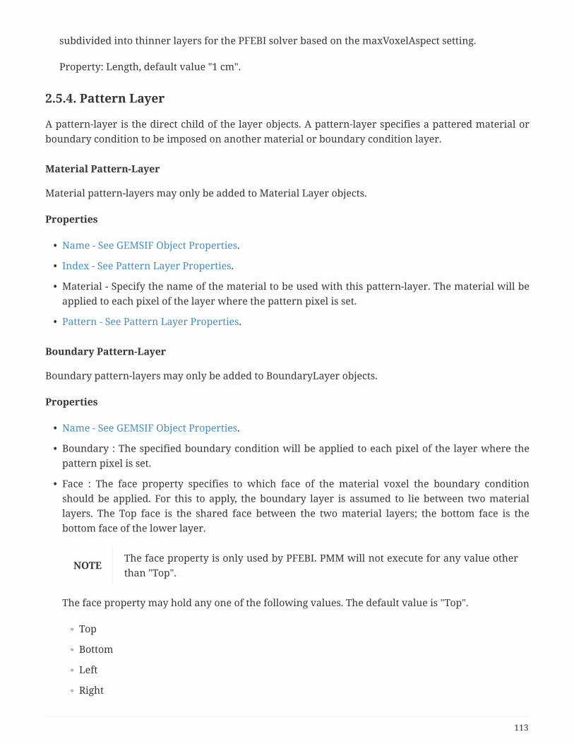
subdivided into thinner layers for the PFEBI solver based on the maxVoxelAspect setting.


2.5.4. Pattern Layer

A pattern-layer is the direct child of the layer objects. A pattern-layer specifies a pattered material orboundary condition to be imposed on another material or boundary condition layer.

Material Pattern-Layer

Material pattern-layers may only be added to Material Layer objects.

Properties


• Index - See Pattern Layer Properties.

• Material - Specify the name of the material to be used with this pattern-layer. The material will beapplied to each pixel of the layer where the pattern pixel is set.

• Pattern - See Pattern Layer Properties.

Boundary Pattern-Layer

Boundary pattern-layers may only be added to BoundaryLayer objects.

Properties


• Boundary : The specified boundary condition will be applied to each pixel of the layer where thepattern pixel is set.

• Face : The face property specifies to which face of the material voxel the boundary conditionshould be applied. For this to apply, the boundary layer is assumed to lie between two materiallayers. The Top face is the shared face between the two material layers; the bottom face is thebottom face of the lower layer.

NOTEThe face property is only used by PFEBI. PMM will not execute for any value otherthan "Top".

The face property may hold any one of the following values. The default value is "Top".

◦ Top

◦ Bottom

◦ Left

◦ Right

113

◦ Front

◦ Back

• index : See Pattern Layer Properties

• pattern : See Pattern Layer Properties

Pattern Layer Properties

Index

Specify the order of the patternlayer. No two pattern-layers that are children of the same layer mayshare the same index value. PatternLayers are applied to the underlying layer in increasing orderstarting at index zero.

When edited through the GUI interface, changing the index of one pattern-layer will update anyother pattern-layers that would share the new index value to prevent conflicts.

Pattern

Name of the pattern to be included in the layer.

2.5.5. Layer Properties

Patterns

A layer includes zero or more pattern objects, each associated with a material or boundary condition.The patterns property contains an array of PatternLayer names.

NOTE The list of patterns must be empty for Material Layers when using the PMM solver.

Position

The position property specifies the layer’s position within the multilayer stack of the unit cell. Thelayer position is a zero-based index, where low indices are at the bottom of the stack. No two layersmay share the same index; when edited in the GUI, positions are automatically updated to ensure thatall layers are provided with a unique index. Direct editing of the property will move other layerpositions in order to accommodate changes made to the select layer.

2.6. ResultsA results file is created for every excitation and is linked to a HDF5 (.hdf) file when a simulation is firstsaved. The HDF5 file contains the results of a simulation after it has been run and will appear in thesame directory that the simulation is saved in. When a simulation is moved, the HDF5 file will need tobe moved as well and relinked in order for the plotted result to display. Otherwise, the simulation willhave to be run again.

An excitation can be validated and run from the results file by right clicking on it. In addition, once a

114

simulation is run, results can be plotted by right clicking the desired results file and selecting "Createplot". If a results file is deleted, it can be recreated by validating or running the correspondingexcitation again.

2.6.1. Results Properties

Name


Enable for Run All

Allows the user to exclude the path excitation from "Run all" commands.

Property: String, default value "true".

Path

Path to results file.

Excitation

Name of the connected excitation.

2.7. General Object Properties

2.7.1. Pattern Constraint

Specify the name of a user-defined Action as a constraint filter on the allowable patterns that may beapplied within the current simulation.

WARNING This property is not yet implemented.

The named action will be called during binary pattern generation with a trial pattern. The action mustreturn a modified pattern that satisfies any design constraints

3. DocksCurrently, PFSS contains a single dock, the Layer Editor Dock.

3.1. Layer EditorThe Layer Editor Dock provides the user with a 2D side view of the layer stack that constructs the unitcell. The dock can be used to select a layer, add a layer, or remove a layer. The dock can also be used toexport an image of the layer stack to the clipboard.

115

3.1.1. Layer Editor Properties

Name


Floating


Location


Next Dock


Pinned


Size


Tabbed


Title


4. ViewsPFSS utilizes both the Action View and the Plot2D view from GEMSIF. For more information on theseviews, see GEMSIF Views.

In addition to the GEMSIF views, PFSS has a Layer Stackup View that displays a 3D model of the layerstack.

4.1. Layer Stackup ViewThe Layer Stackup View provides a 3D rendering of the layer stack. Each layer is rendered based onthe color and transparency of the material or boundary condition.

116

The user can freely rotate the 3D model, add axes, and dimensions. The 3D model can be saved andprinted from this view as well.

Selecting a layer will open the layer’s object if the Property Editor Dock is open, allowing the user toeasily edit the layer. The user can turn off either type of layer, allowing for easier selection or viewingof a particular type of layer.

4.1.1. Stackup View Properties

Name


Window Geometry

See GEMSIF View Properties - Window Geometry.

Window State

See GEMSIF View Properties - Window State.

Window Visible

See GEMSIF View Properties - Window Visible.

Axes Visible

Enables visible axes on the 3D model. Value is true or false.

Boundaries Visible

Turns visible Boundary Condition Layers on or off. Value is true or false.

Dimensions Visible

Enable dimensions on the 3D model. Value is true or false.

Expansion Factor

Configure the layers within the simulation to be separated by a percentage factor relative to the totalunit cell thickness. The expansion factor is 0 by default, which corresponds to no expansion. With noexpansion, all layers are displayed as simulated. The view can be expanded for better visualization byincreasing the expansion factor to 100 (interpreted as percent) or more.

Materials Visible

Turns visible Material Layers on or off. Value true or false.

117

rulerVisible

Displays a ruler if enabled. True or false.

Title

See GEMSIF View Properties - Title

118

User Manual for PFSS

1. Introduction to PFSSThe PFSS tool is used to rapidly and efficiently solve the problem of electromagnetic scattering fromperiodic, 2.5D structures for any incidence angle or polarization. The software is suitable for designingdevices for RF, terahertz, infrared, and optical applications. As a specialized simulation tool, the solverswithin PFSS can rapidly compute the scattering properties from periodic metallodielectric frequencyselective surfaces, metamaterials, and antennas. The efficient nature of the solvers allows the use ofGEMSIF’s advanced stochastic optimizers to select the design properties.

1.1. FeaturesThe simulation capabilities of the PFSS tool are summarized in the list below. Details on the capabilitiesof the individual solvers PMM and PFEBI are also available.

• Doubly-periodic rectangular multilayered unit cells

• Fast, efficient calculation of scattering parameters from complex, inhomogeneous layered media

• Tight integration with optimization algorithms

• Plane wave incidence angular sweeps in theta and phi

• Frequency sweeps

• Dual-polarization excitation with cross-polarized reflection and transmission analysis

• Absorptivity and emissivity analysis

• Homogeneous and inhomogeneous material and boundary condition layers

• Isotropic, anisotropic, and bianisotropic dielectric materials

• Isotropic magnetic materials

• Lossy and lossless dielectric and magnetic materials

• Dispersive and nondispersive materials

• Integration with GEMSIF material database

• Parallel and series RLC lumped elements

• Surface impedance boundary conditions across any voxel face

• Thoroughly tested and validated simulation kernels

1.2. Simulation ModelEach simulation model is represented by a single, rectangular cuboid unit cell consisting of one or

119

more volumetric layers of dielectric media that are (optionally) separated by planar layers of a specificboundary condition. Available boundary conditions include perfect electric conductors, surfaceimpedance, lumped elements, and surface impedance calculated for specific permittivity andpermeability. PFSS supports isotropic, anisotropic, and bianisotropic materials with optional frequencydispersion. The individual layers are discretized into collections of rectangular pixels, where thematerial properties or boundary condition of each pixel may be independently specified. Layers maybe homogeneous or inhomogeneous depending on the solver, and boundary conditions may also bespecified on any faces of a volumetric material voxel, which allows for the modeling of vias and other2.5D structures.

Figure 4. Geometry of multilayer metallodielectric geometry.

120

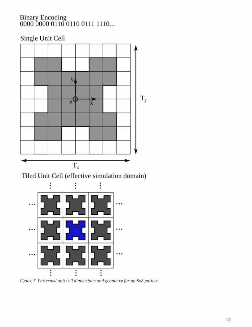
Figure 5. Patterned unit cell dimensions and geometry for an 8x8 pattern.

121

Figure 6. Demonstration pixel patterns.

Periodic boundary conditions are used for the x- and y-faces of the simulation domain, which allows asimulation of a single unit cell to accurately predict the electromagnetic response of an infinite array ofunit cells. The response of a finite array of unit cells, as the array size becomes large, converges to theresponse of the infinite tiling. Commonly, 10-50 unit cells can be considered to have a bulk behaviorwhere the periodic simulation results are an accurate predictor of the finite array response. Theperiodic unit cell response is most accurate for the unit cells in the center of the array, while it is lessvalid for elements on the boundaries of the array. For a large array, however, the response of the edgeelements is generally unimportant for the behavior of the array as a whole, and the bulk, effectiveresponse of the periodic unit cell may be accurately applied.

122

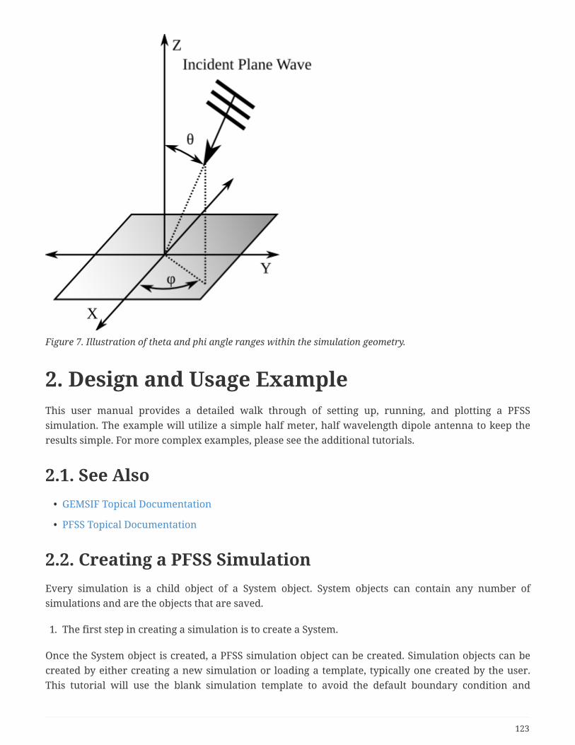
Figure 7. Illustration of theta and phi angle ranges within the simulation geometry.

2. Design and Usage ExampleThis user manual provides a detailed walk through of setting up, running, and plotting a PFSSsimulation. The example will utilize a simple half meter, half wavelength dipole antenna to keep theresults simple. For more complex examples, please see the additional tutorials.

2.1. See Also• GEMSIF Topical Documentation

• PFSS Topical Documentation

2.2. Creating a PFSS SimulationEvery simulation is a child object of a System object. System objects can contain any number ofsimulations and are the objects that are saved.

1. The first step in creating a simulation is to create a System.

Once the System object is created, a PFSS simulation object can be created. Simulation objects can becreated by either creating a new simulation or loading a template, typically one created by the user.This tutorial will use the blank simulation template to avoid the default boundary condition and

123

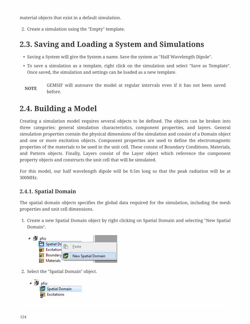
material objects that exist in a default simulation.

2. Create a simulation using the "Empty" template.

2.3. Saving and Loading a System and Simulations• Saving a System will give the System a name. Save the system as "Half Wavelength Dipole".

• To save a simulation as a template, right click on the simulation and select "Save as Template".Once saved, the simulation and settings can be loaded as a new template.

NOTEGEMSIF will autosave the model at regular intervals even if it has not been savedbefore.

2.4. Building a ModelCreating a simulation model requires several objects to be defined. The objects can be broken intothree categories: general simulation characteristics, component properties, and layers. Generalsimulation properties contain the physical dimensions of the simulation and consist of a Domain objectand one or more excitation objects. Component properties are used to define the electromagneticproperties of the materials to be used in the unit cell. These consist of Boundary Conditions, Materials,and Pattern objects. Finally, Layers consist of the Layer object which reference the componentproperty objects and constructs the unit cell that will be simulated.

For this model, our half wavelength dipole will be 0.5m long so that the peak radiation will be at300MHz.

2.4.1. Spatial Domain

The spatial domain objects specifies the global data required for the simulation, including the meshproperties and unit cell dimensions.

1. Create a new Spatial Domain object by right clicking on Spatial Domain and selecting "New SpatialDomain".

2. Select the "Spatial Domain" object.

124

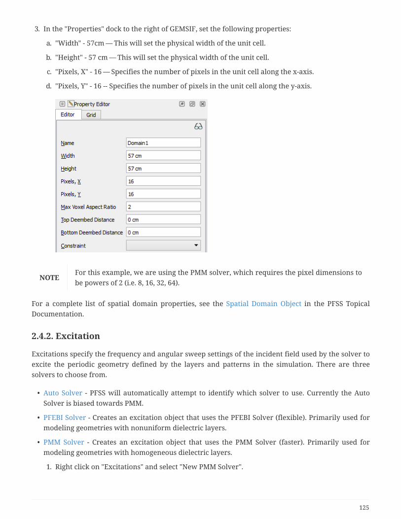
3. In the "Properties" dock to the right of GEMSIF, set the following properties:

a. "Width" - 57cm — This will set the physical width of the unit cell.

b. "Height" - 57 cm — This will set the physical width of the unit cell.

c. "Pixels, X" - 16 — Specifies the number of pixels in the unit cell along the x-axis.

d. "Pixels, Y" - 16 -- Specifies the number of pixels in the unit cell along the y-axis.

NOTEFor this example, we are using the PMM solver, which requires the pixel dimensions tobe powers of 2 (i.e. 8, 16, 32, 64).

For a complete list of spatial domain properties, see the Spatial Domain Object in the PFSS TopicalDocumentation.

2.4.2. Excitation

Excitations specify the frequency and angular sweep settings of the incident field used by the solver toexcite the periodic geometry defined by the layers and patterns in the simulation. There are threesolvers to choose from.

• Auto Solver - PFSS will automatically attempt to identify which solver to use. Currently the AutoSolver is biased towards PMM.

• PFEBI Solver - Creates an excitation object that uses the PFEBI Solver (flexible). Primarily used formodeling geometries with nonuniform dielectric layers.

• PMM Solver - Creates an excitation object that uses the PMM Solver (faster). Primarily used formodeling geometries with homogeneous dielectric layers.

1. Right click on "Excitations" and select "New PMM Solver".

125

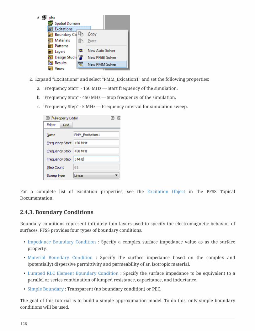
2. Expand "Excitations" and select "PMM_Exication1" and set the following properties:

a. "Frequency Start" - 150 MHz — Start frequency of the simulation.

b. "Frequency Stop" - 450 MHz — Stop frequency of the simulation.

c. "Frequency Step" - 5 MHz — Frequency interval for simulation sweep.

For a complete list of excitation properties, see the Excitation Object in the PFSS TopicalDocumentation.

2.4.3. Boundary Conditions

Boundary conditions represent infinitely thin layers used to specify the electromagnetic behavior ofsurfaces. PFSS provides four types of boundary conditions.

• Impedance Boundary Condition : Specify a complex surface impedance value as as the surfaceproperty.

• Material Boundary Condition : Specify the surface impedance based on the complex and(potentially) dispersive permittivity and permeability of an isotropic material.

• Lumped RLC Element Boundary Condition : Specify the surface impedance to be equivalent to aparallel or series combination of lumped resistance, capacitance, and inductance.

• Simple Boundary : Transparent (no boundary condition) or PEC.

The goal of this tutorial is to build a simple approximation model. To do this, only simple boundaryconditions will be used.

126

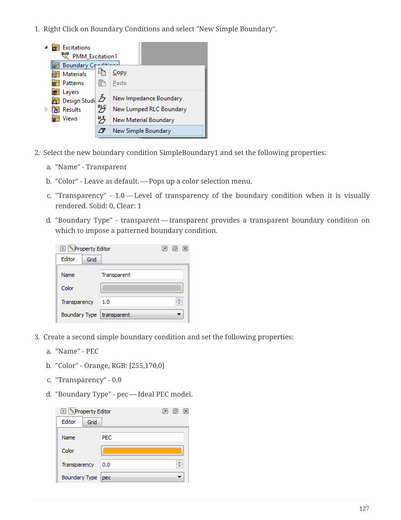
1. Right Click on Boundary Conditions and select "New Simple Boundary".

2. Select the new boundary condition SimpleBoundary1 and set the following properties:

a. "Name" - Transparent

b. "Color" - Leave as default. — Pops up a color selection menu.

c. "Transparency" - 1.0 — Level of transparency of the boundary condition when it is visuallyrendered. Solid: 0, Clear: 1

d. "Boundary Type" - transparent — transparent provides a transparent boundary condition onwhich to impose a patterned boundary condition.

3. Create a second simple boundary condition and set the following properties:

a. "Name" - PEC

b. "Color" - Orange, RGB: [255,170,0]

c. "Transparency" - 0.0

d. "Boundary Type" - pec — Ideal PEC model.

127

For a complete list of boundary condition properties, see the Boundary Condition Object in the PFSSTopical Documentation.

2.4.4. Material

Material objects represent the properties of dielectric or magnetic materials for the PFSS solvers.

1. Right click on Materials and select "New Material"

2. Select the new material Material1 and set the following properties:

a. "Name" - Vacuum

b. "Color" - Leave as default.

c. "Transparency" - Leave as default.

d. Add the following Field Definitions:

i. "Isotropic Permittivity" - 1

ii. "Isotropic Permeability" - 1

128

For a complete list of material properties, see the Material Object in the GEMSIF TopicalDocumentation.

2.4.5. Pattern

A pattern is a rectangular array or image of boolean values that may be either true or false. Each valueis associated with a pixel. The pattern determines how a boundary condition or material will berendered in the model.

1. Right-click "Patterns" and select "New Binary".

2. Expand "Patterns" and then select the "BinaryPattern1" object to select it.

3. The setting and a pattern editor should appear in the Properties Dock. Set the following properties:

a. "Name" - patchesPattern

b. Set the two "Grid Size" values to 16

c. "Symmetry" - Ref90

4. Click on the pixels (gray squares) in the pattern to form a vertical dipole about the center, leavingthe top and bottom row of pixels empty

129

NOTEUse the buttons just above and to the right of the pattern editor to switchbetween setting pixels, toggling pixels, and clearing pixels. In the default setting pixelmode, left clicking selects a pixel, right clicking deselects a pixel.

For a complete list of pattern properties, see the Pattern Object in the PFSS Topical Documentation.

2.4.6. Layers

Layers combine general properties and component properties to build a unit cell to simulate.

• Material Layer : Patterned or unpatterned dielectric layer of finite thickness.

• Boundary Layer : Patterned or unpatterned boundary condition (PEC, Impedance, lumpedelement).

1. Right-click "Layers" and click "New Material Layer." Expand "Layers" and select the new"MaterialLayer1".

2. Set the following properties:

130

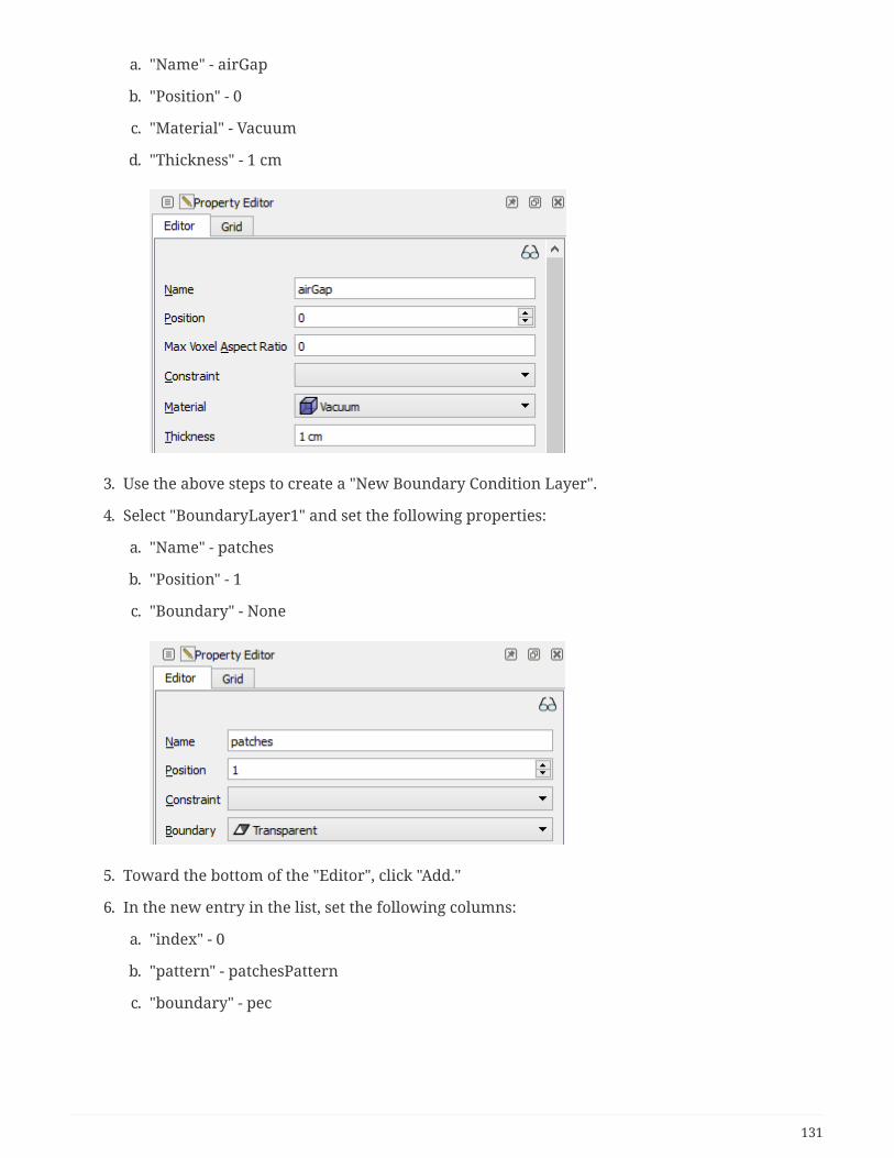
a. "Name" - airGap

b. "Position" - 0

c. "Material" - Vacuum

d. "Thickness" - 1 cm

3. Use the above steps to create a "New Boundary Condition Layer".

4. Select "BoundaryLayer1" and set the following properties:

a. "Name" - patches

b. "Position" - 1

c. "Boundary" - None

5. Toward the bottom of the "Editor", click "Add."

6. In the new entry in the list, set the following columns:

a. "index" - 0

b. "pattern" - patchesPattern

c. "boundary" - pec

131

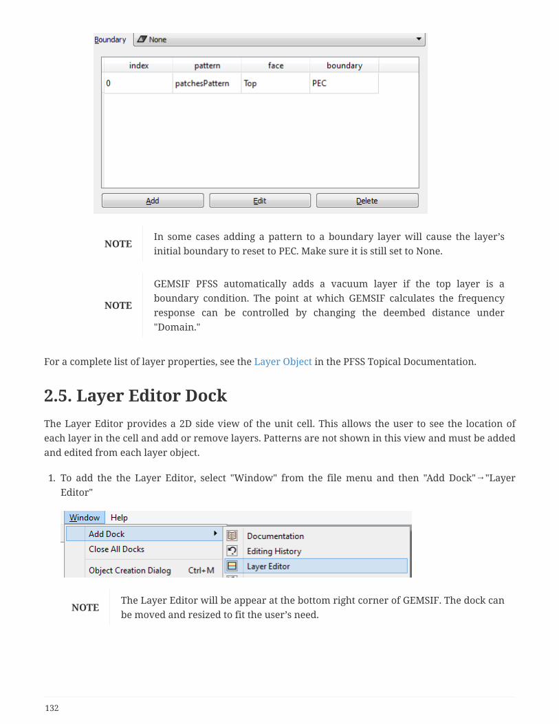
NOTEIn some cases adding a pattern to a boundary layer will cause the layer’sinitial boundary to reset to PEC. Make sure it is still set to None.

NOTE

GEMSIF PFSS automatically adds a vacuum layer if the top layer is aboundary condition. The point at which GEMSIF calculates the frequencyresponse can be controlled by changing the deembed distance under"Domain."

For a complete list of layer properties, see the Layer Object in the PFSS Topical Documentation.

2.5. Layer Editor DockThe Layer Editor provides a 2D side view of the unit cell. This allows the user to see the location ofeach layer in the cell and add or remove layers. Patterns are not shown in this view and must be addedand edited from each layer object.

1. To add the the Layer Editor, select "Window" from the file menu and then "Add Dock"→"LayerEditor"

NOTEThe Layer Editor will be appear at the bottom right corner of GEMSIF. The dock canbe moved and resized to fit the user’s need.

132

2.5.1. Layer Editor Controls

• : Toggle dimension lines.

• : Toggle in-layer text.

• : Adds a material layer above the selected layer.

• : Adds a boundary layer above the selected layer.

• : Adds a material layer below the selected layer.

• : Adds a boundary layer below the selected layer.

• : Deletes the selected layer.

• : Saves a snapshot of the editor to the clipboard.

NOTE Right clicking on a layer will also provide the same options as the controls.

133

2.6. Layer Stackup ViewPFSS provides a Layer Stackup View to view a 3D rendering of the unit cell.

1. Right click on "Views" at the bottom of the Hierarchy Tree and select New Layer Stackup.

2. Clicking on the view and holding will allow you to rotate the model.

134

Selecting a layer in the Stackup View will load the editor for the layer in the Property Editor Dock forquick editing.

Using the menu options, the view can be saved as an image or exported to the clipboard. Axes anddimensions can also be added.

2.6.1. Validating and Running

1. After building a simulation, it needs to be saved before it can be run. This is required to link theexcitation object to the results file. For future changes, saving is not required, but it isrecommended.

2. Next, the simulation should be verified. This is a useful check to ensure that the simulation is freefrom errors. While not required, validating is recommended.

a. Right click on "PMM_Excitation1" and select "Validate". If there are multiple excitations, theycan be validated at the same time by right clicking on the simulation object (the name) andselecting "Validate all Excitations."

b. A properly validated simulation will provide no errors in the "Status" dock.

3. Now that the simulation has been validated, it can now be run. For later changes to the simulation,it is not necessary to validate the simulation unless you want to check for errors.

a. Right click on "PMM_Excitation1" and select "Run."

135

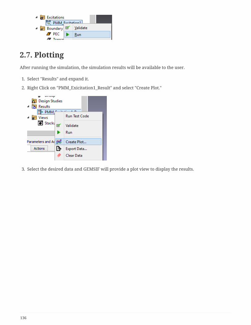
2.7. PlottingAfter running the simulation, the simulation results will be available to the user.

1. Select "Results" and expand it.

2. Right Click on "PMM_Exicitation1_Result" and select "Create Plot."

3. Select the desired data and GEMSIF will provide a plot view to display the results.

136

3. SolversTwo solvers are included in the PFSS package, each specialized for a particular design problem. PMMis based on the method of moments formulation, and so has limited support for complex,inhomogeneous material parameters but is extremely rapid to execute. In comparison, the PFEBIsolver based on a hybridized finite element-boundary integral solver has fewer geometrical limitationsand supports nearly arbitrary designs specified on the voxel grid, but is generally slower than thePMM tool. The PFSS tool will by default automatically select the best solver for a given modeldepending on the specified geometry and other model requirements, but the user can request aspecific solver, as well.

3.1. PMMThe Periodic Method of Moments (PMM) is an FFT-accelerated method of moments solver specializedto periodic, multilayered dielectric structures separated by patterned layers of metallic or surface-impedance boundary conditions.

PMM uses the spectral-domain Method of Moments accelerated with the fast Fourier transform (FFT)to analyze the problem of scattering from a frequency selective surface (FSS). The solver computes theelectric current distribution on a single unit cell of a doubly-periodic structure in order to determinethe resulting scattered fields. The FSS is printed on a dielectric substrate and covered by an additional

137

superstrate layer. This configuration can be optionally backed by a PEC ground plane. In addition,multiple such screens may be cascaded to form a multilayer metallo-dielectric stack. The superstrateand substrate can be either lossy or lossless materials. The metallic FSS screen may be modeled as aperfectly-electrically conducting screen, or as possessing a specified surface impedance. The reflectionand transmission coefficients may be calculated for incident fields for both polarizations (TE and TMcases).

3.1.1. Solver Implementation and Limitations

The solver and its outputs have been thoroughly verified and validated against analytical solutions andthe outputs of other simulation tools; please see the papers cited in the PMM References. A descriptionof the mathematical underpinnings and limitations of the solver are listed below.

• Only a single unit cell of the periodic structure must be discretized.

• The number of pixels in the x- and y-directions must be integer powers of 2 (8, 16, 32, etc.)

• The discretization of the unit cell of the FSS should approximately satisfy the followingrequirements: max(Δx, Δy) < λ/10.

• Isolated pixels or pixels that are only connected via a diagonal are not allowed in PMM. The MoMbasis functions extend over two adjacent pixels with the same boundary conditions, so an isolatedpixel (or an isolated hole) will not produce accurate results. Note that the PFEBI solver is notsubject to this limitation. Also, setting the oversample factor of the excitation to any value greaterthan unity will also resolve the issue.

138

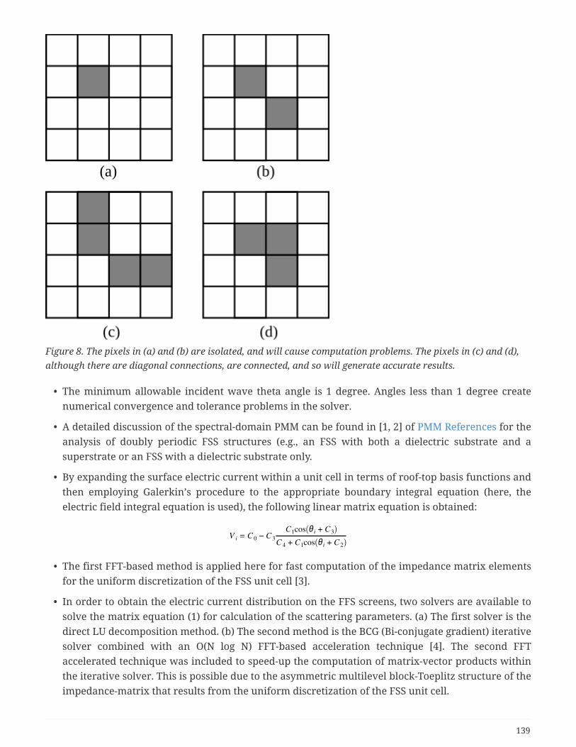
Figure 8. The pixels in (a) and (b) are isolated, and will cause computation problems. The pixels in (c) and (d),although there are diagonal connections, are connected, and so will generate accurate results.

• The minimum allowable incident wave theta angle is 1 degree. Angles less than 1 degree createnumerical convergence and tolerance problems in the solver.

• A detailed discussion of the spectral-domain PMM can be found in [1, 2] of PMM References for theanalysis of doubly periodic FSS structures (e.g., an FSS with both a dielectric substrate and asuperstrate or an FSS with a dielectric substrate only.

• By expanding the surface electric current within a unit cell in terms of roof-top basis functions andthen employing Galerkin’s procedure to the appropriate boundary integral equation (here, theelectric field integral equation is used), the following linear matrix equation is obtained:

• The first FFT-based method is applied here for fast computation of the impedance matrix elementsfor the uniform discretization of the FSS unit cell [3].

• In order to obtain the electric current distribution on the FFS screens, two solvers are available tosolve the matrix equation (1) for calculation of the scattering parameters. (a) The first solver is thedirect LU decomposition method. (b) The second method is the BCG (Bi-conjugate gradient) iterativesolver combined with an O(N log N) FFT-based acceleration technique [4]. The second FFTaccelerated technique was included to speed-up the computation of matrix-vector products withinthe iterative solver. This is possible due to the asymmetric multilevel block-Toeplitz structure of theimpedance-matrix that results from the uniform discretization of the FSS unit cell.

139

• Upon solving the matrix equation (1), the reflection and transmission coefficients are calculatedbased on the zeroth order scattered harmonic.

• This program is developed based on the code written by Joseph D. Vacchione.

3.1.2. References

The papers referenced below include background material [1-4] on the algorithms used by the PMMtool, as well as references on the development, testing, validation, and usage for example designs ofthe PMM solver [5-10].

1. L. Li, D. H. Werner, J. A. Bossard, and T. S. Mayer, “A Model-based parameter estimation techniquefor wideband interpolation of periodic moment method impedance matrices with application togenetic algorithm optimization of frequency selective surfaces,” IEEE Trans. Antennas Propagat.,vol.54, no.3, pp.908–924, 2006.

2. C. H. Chan, “Analysis of frequency selective surfaces,” in Frequency Selective Surface and GridArray, T. K. Wu, Eds., Chap. 2, New York: Wiley, 1995.

3. J. D. Vacchione, “Techniques for analyzing planar, periodic, frequency selective surface systems,”Ph.D. Dissertation, University of Illinois at Urbana-Champaign, 1990.

4. B. E. Barrowes, F. L. Teixeira, and J. A. Kong, “Fast algorithm for matrix-vector multiply ofasymmetric multilevel block-Toeplitz matrices in 3-D scattering,” Microwave Opt. Technol. Lett.,vol. 31, no. 1, pp. 28–32, 2001.

5. Xiande Wang and Douglas H. Werner, “Improved model-based parameter estimation approach foraccelerated periodic method of moments solutions with application to the analysis of convolutedfrequency selected surfaces and metamaterials,” IEEE Transactions on Antennas and Propagation,Vol. 58, No. 1, pp. 122-131, January 2010.

6. Z. Bayraktar, M. D. Gregory, X. Wang, and D. H. Werner, "Matched Impedance Thin PlanarComposite Magneto-dielectric Metasurfaces," IEEE Transactions on Antennas and Propagation, Vol.60, No. 4, pp. 1910 - 1920, April 2012

7. Z. Bayraktar, X. Wang, and D. H. Werner, "Thin Composite Matched Impedance Magneto-DielectricMetamaterial Absorbers," Proceedings of the 2010 IEEE International Symposium on Antennas andPropagation and USNC/URSI National Radio Science Meeting, Toronto, Canada, July 11-17, 2010.

8. X. Wang and D. H. Werner, "Improved Model-Based Parameter Estimation Approach forAccelerated Periodic Method of Moments Solutions with Application to the Analysis of ConvolutedFrequency Selective Surfaces and Metamaterials," IEEE Transactions on Antennas and Propagation,Vol. 58, Issue 1, pp. 122-131, January 2010.

9. X. Wang and D. H. Werner, "Multiband Ultra-Thin Electromagnetic Band-Gap and Double-SidedWideband Absorbers Based on Resistive Frequency Selective Surfaces," Proceedings of the 2009IEEE International Symposium on Antennas and Propagation and USNC/URSI National RadioScience Meeting, Charleston, SC, USA, June 1-5, 2009.

10. X. Wang and D. H. Werner, "Accelerated PMM Solutions via Model-Based Parameter Estimation andFast Fourier Transform Techniques," Proceedings of the 2008 IEEE AP-S International Symposium

140

and USNC/URSI National Radio Science Meeting in San Diego, CA, USA, July 5-11, 2008

3.2. PFEBIThe Periodic Finite-Element Boundary-Integral (PFEBI) solver is more general than the PMM solver, asit allows inhomogeneous material layers and boundary conditions to be applied to any face of a voxel.The PFEBI solver is made available under license from the Penn State Research Foundation (PSRF).

The PFEBI solver analyses the scattering or radiation from a double-periodic structure. This periodicstructure may be a Frequency Selective Surface (FSS), metamaterial, metasurface, or infinite antennaarray. In both cases, the structure is composed of (1) one or more homogeneous dielectric slabs(isotropic, anisotropic, or bi-anisotropic), (2) one or more inhomogeneous dielectric slabs, and (3) oneor more metal or surface impedance boundary condition screens. Dielectric media may be lossy,lossless, and/or dispersive. Active (gain) materials are not allowed. Isotropic metallic materials mayalso be modelled. Metal screens may be modelled as PEC or as a potentially lossy surface impedance.

Scattering parameters are computed for FSS problems and the input impedance and radiation (Gain)pattern are calculated for antenna problems.

3.2.1. Solver Implementation and Limitations

The PFEBI solver uses the hybrid finite-element boundary-integral (FEBI) method to numericallycompute the electric field inside and on the surface of the structure. The solver and its outputs havebeen thoroughly verified and validated against analytical solutions and the outputs of other simulationtools; please see the papers cited in the PFEBI References. A description of the mathematicalunderpinnings and limitations of the solver are listed below.

• Only a single unit cell of the doubly-periodic structure is modelled.

• The number of pixels in the x and y directions may be any positive integer, including 1, and may bedifferent. Geometries that are periodic along one axis, but infinite along the other may be specifiedby only a single pixel in the infinite direction.

• The discretization of the unit cell should approximately satisfy the following requirements: a)max(Δx, Δy, Δz) < λε/10, and b) Δx/ Δy/ Δz ~= 1.0 That is, each voxel dimension should be smallerthan a tenth of a wavelength in the highest-index material in the simulation, and the voxels shouldbe approximately cubic.

• PFEBI uses brick elements for finite-element volumetric discretization and uses roof-top functionfor top and bottom surface discretization. Galerkin’s method is used for testing in the boundary-integral calculation. In order to increase computation efficiency, symmetries in calculating theentries of the impedance matrix in boundary-integral part (only for normal incidenec case) and infinite-element part are fully exploited in the programming. This requires that all the elements areof the same dimensions.

• The BCG-FFT (Fast Fourier Transform) algorithm has been included in the FEBI-code to speed-upthe computation of matrix-vector for BI part due to a BI sub-matrix with a Toeplitz-Block Toeplitz

141

structure.

• For the boundary-integral part, the conventional free-space Green’s function becomes an infinitedouble summation (periodic Green’s function), and the Ewald transformation technique is used toaccelerate the convergence of the double summation. The Ewald transformation converts theoriginal periodic Green’s functions into two parts, one in spatial domain and one in spectraldomain, both of which converges at a much faster speed.

• PFEBI uses the Mixed Potential Integral Equation (MPIE) and solves for the total electric field insidethe structure and the tangential electric on the surface of the structure. For Isotropic materials, thepertinent MPIE formulation is given by:

For the general case of inhomogeneous and lossy bi-anisotropic materials characterized by thefollowing constitutive relations:

The pertinent MPIE formulation is given as follows:

• For FSS scattering problem, the reflection and transmission coefficients are calculated byperforming the FFT of the tangential electric field on the top and bottom surface of the unit cell.Generally speaking, the FFT computes the scattering matrix of the periodic structure, with thecenter entry being the reflection/transmission coefficients (for oblique incidence, phasecompensation is required before performing the FFT). Although the FFT is most efficient when thenumber of pixels in the x and y directions are integer powers of 2, the PFEBI solver supports anypixel dimensions, including 1 x 1.

3.2.2. References

The papers referenced below include background material [1-4] on the algorithms used by the PFEBItool, as well as references on the development, testing, validation, and usage for example designs ofthe PFEBI solver [5-27].

1. J. L. Volakis, A. Chatterjee, and L. C. Kempel, Finite Element Method for Electromagnetics, IEEEPress, 1998.

2. T. F. Eibert, J. L. Volakis, D. R. Wilton, and D. R. Jackson, “Hybrid FE/BI modeling of 3-D doublyperiodic structures utilizing triangular prismatic elements and an MPIE formulation accelerated bythe Ewald transformation”, IEEE Trans. Antennas and Propag., vol. 47, no. 5, pp. 843-850, May 1999.

3. J. Jin, The Finite Element Method in Electromagnetics, John Wiley, 2002.

4. F. Bilotti, L. Vegni, and A. Toscano, “Radiation and scattering feature of patch antennas withbianisotropic substrates,”

5. Xiande Wang, Douglas H. Werner and Jeremiah P. Turpin, “Application of AIM and MBPEtechniques to accelerate modeling of 3-D doubly periodic structures with non-orthogonal latticescomposed of bianisotropic media,” Accepted for publication in IEEE Transactions on Antennas andPropagation, Vol. 62, No. 8, Aug. 2014. (triangular-based)

142

6. J. Ashbach, X. Wang, and D. H. Werner, "The Finite Element Boundary Integral Method AcceleratedUsing a Graphics Processing Unit," Proceedings of the 2013 IEEE International Symposium onAntennas & Propagation and USNC/URSI National Radio Science Meeting, July 7-13, 2013, Orlando,FL, USA. (triangular-based).

7. J. Ashbach, J. A. Bossard, X. Wang, and D. H. Werner, "Metamaterial Absorber for the Near-IR withCurvilinear Geometry based on Beziér Surfaces," Proceedings of the 2013 IEEE InternationalSymposium on Antennas & Propagation and USNC/URSI National Radio Science Meeting, July 7-13,2013, Orlando, FL, USA. (triangular-based)

8. Q. Wu, C. P. Scarborough, B. G. Martin, R. K. Shaw, D. H. Werner, E. Lier, and X. Wang, "A Ku-bandDual Polarization Hybrid-Mode Horn Antenna Enabled by Printed-Circuit-Board Metasurfaces,"IEEE Transactions on Antennas and Propagation, Vol. 61, No. 3, pp. 1089-1098, Mar. 2013.

9. Q. Wu, C. P. Scarborough, D. H. Werner, E. Lier, and X. Wang, "Design Synthesis of Metasurfaces forBroadband Hybrid-mode Horn Antennas with Enhanced Radiation Pattern and PolarizationCharacteristics," IEEE Transactions on Antennas and Propagation, Vol. 60, No. 8, pp. 3594-3604, Aug.2012.

10. Z. Bayraktar, J. A. Bossard, X. Wang, and D. H. Werner, "A Real-valued Parallel Clonal SelectionAlgorithm and Its Application to the Design Optimization of Multi-layered Frequency SelectiveSurfaces," IEEE Transactions on Antennas and Propagation, Vol. 60, No. 4, pp. 1831 - 1843, April2012.

11. Z. Bayraktar, M. D. Gregory, X. Wang, and D. H. Werner, "A Versatile Design Strategy for ThinComposite Planar Double-Sided High-Impedance Surfaces," IEEE Transactions on Antennas andPropagation, Vol. 60, No. 6, pp. 2770-2780, June 2012.

12. Q. Hao, Y. Zeng, B. K. Juluri, X. Wang, B. Kiraly, I-K. Chiang, L. Jensen, D. H. Werner, V. H. Crespi andT. J. Huang, "Metallic Membranes with Subwavelength Complementary Patterns: Distinct Substratesfor Surface-Enhanced Raman Scattering," ACS Nano, Vol. 5, No. 7, pp. 5472-5477, July 2011.

13. M. Gregory, X. Wang, and D. H. Werner, "Flexible Design of Doubly Periodic Frequency SelectiveSurfaces with a Prismatic Mesh Based FEBI Simulation Tool and CMA-ES," Proceedings of the 2011IEEE International Symposium on Antennas and Propagation and USNC/URSI National RadioScience Meeting, Spokane, WA, USA, July 3-8, 2011.

14. Y. Zeng, X. Wang, D. H. Werner, Q. Hao, and T. Huang, "Linear Optical and Surface-enhanced RamanScattering Study on Metallic Membranes with Subwavelength Complementary Patterns,"Proceedings of the 2011 IEEE International Symposium on Antennas and Propagation andUSNC/URSI National Radio Science Meeting, Spokane, WA, USA, July 3-8, 2011.

15. Z. Jiang, J. A. Bossard, X. Wang, and D. H. Werner, "Synthesizing Metamaterials with AngularlyIndependent Effective Medium Properties Based on an Anisotropic Parameter Retrieval TechniqueCoupled with a Genetic Algorithm," Journal of Applied Physics, Vol. 109, pp. 013515/1-11, 2011.

16. Q. Hao, Y. Zeng, X. Wang, Y. Zhao, B. Wang, D. H. Werner, V. H. Crespi, and T. J. Huang,"Characterization of Complementary Patterned Metallic Membranes Produced Simultaneously by aDual Fabrication Process," Applied Physics Letters, Vol. 97, 193101, 2010.

17. D. H. Werner, Z. H.. Jiang, F. Toor, S. Yun, Z. Bayraktar, X. Wang, T. Mayer, and P. L. Werner,

143

"Metamateria Absorbers with Wide-Angle Polarization-Insensitive Multiband Properties for RFthrough Mid-Infrared Applications," the Fourth International Congress on AdvancedElectromagnetic Materials in Microwaves and Optics, Karlsruhe, Germany, September 12-16, 2010.

18. X. Wang and D. H. Werner, "Fast Analysis of 3-D Doubly Periodic Structures with ComplexGeometry and Anisotropic Materials using the Adaptive Integral Method," Proceedings of the 2010IEEE International Symposium on Antennas and Propagation and USNC/URSI National RadioScience Meeting, Toronto, Canada, July 11-17, 2010.

19. Z. H. Jiang, Q. Wu, X. Wang, and D. H. Werner, "Flexible Wide-Angle Polarization-Insensitive Mid-Infrared Metamaterial Absorbers," Proceedings of the 2010 IEEE International Symposium onAntennas and Propagation and USNC/URSI National Radio Science Meeting, Toronto, Canada, July11-17, 2010.

20. Z. H. Jiang, J. A. Bossard, X. Wang, and D. H. Werner, "Genetic Algorithm Synthesis of Impedance-Matched Infrared ZIMs with Wide FOV Using a Generalized Inversion Algorithm," Proceedings ofthe 2010 IEEE International Symposium on Antennas and Propagation and USNC/URSI NationalRadio Science Meeting, Toronto, Canada, July 11-17, 2010

21. Z. Bayraktar, J. A. Bossard, X. Wang, and D. H. Werner, "Real-Valued Parallel Clonal SelectionAlgorithm for Design Optimization in Electromagnetics," Proceedings of the 2010 IEEEInternational Symposium on Antennas and Propagation and USNC/URSI National Radio ScienceMeeting, Toronto, Canada, July 11-17, 2010.

22. X. Wang, D. H. Werner, and D. -H. Kwon, "Acceleration of Periodic FEBI Simulations for General Bi-anisotropic Media Using a Model-Based Parameter Estimation Technique," Proceedings of the 2008IEEE AP-S International Symposium and USNC/URSI National Radio Science Meeting in San Diego,CA, USA, July 5-11, 2008.

23. X. Wang, D. -H. Kwon, D. H. Werner, and I. -C. Khoo, "Anisotropic Liquid Crystals for Tunable OpticalNegative-Index Metamaterials," Proceedings of the 2008 IEEE AP-S International Symposium andUSNC/URSI National Radio Science Meeting in San Diego, CA, USA, July 5-11, 2008.

24. D.-H. Kwon, X. Wang, Z. Bayraktar, B. Weiner, and D. H. Werner, "Reconfigurabletransmissive/Reflective Metamaterial Slab in the Near IR," Proceedings of the 2008 IEEE AP-SInternational Symposium and USNC/URSI National Radio Science Meeting in San Diego, CA, USA,July 5-11, 2008.

25. D.-H. Kwon, X. Wang, Z. Bayraktar, B. Weiner, and D. H. Werner, "Near-Infrafed Metamaterial Filmswith Reconfigurable Transmissive/Reflective Properties," Optics Letters, Vol. 33, No. 6, pp. 545-547,March 15, 2008.

26. X. Wang, D.H. Kwon, D. H. Werner, I.-C. Khoo, Alexander V. Kildishev and Vladimir M. Shalaev,"Tunable Optical Negative-Index Metamaterials Employing Anisotropic Liquid Crystals," AppliedPhysics Letters, 91, 143122, 2007.

27. M. G. Bray, X. Wang, and D. H. Werner, "Dispersive Chiral Frequency Selective Surfaces Simulatedvia FEBI and FDTD," Proceedings of the 2007 IEEE Antennas and Propagation Society InternationalSymposium, Honolulu, Hawaii, USA, pp. 2538-2541, June 10-15, 2007.

144

License for GEMSIF

1. Software Licensing

1.1. E x H SoftwareGEMSIF is provided to users under the terms of the license agreement signed or agreed to when thesoftware was purchased or downloaded. The license agreement with E x H pertains to the software,documentation, images of the software, and E x H-provided solver plugins. The license does not applyto any outputs of the program, and saved files, or simulation results, which are owned solely by theuser of the software. GEMSIF makes use of third-party libraries, each of which is provided under theterms of its own license. These licenses do not affect the use of GEMSIF tool or its outputs, but solelyaffect the rights of E x H to use and distribute the third-party libraries as part of a proprietary softwareproduct.

1.2. Third-Party Libraries and AcknowledgementsGEMSIF makes use of a number of third-party open-source libraries and tools during development,testing, and distribution. These libraries are listed below. This acknowledgement is considered to bethe notification of license rights of users of the GEMSIF software due to the inclusion of these open-source tools. E x H, Inc. does not claim ownership or rights other than those granted by the providedlicenses to any of these third-party software tools. No warranty or guarantee of usefulness orcorrectness is given by the owners of any of these licensed tools.

THIS SOFTWARE IS PROVIDED ``AS IS'' AND ANY EXPRESSED OR IMPLIED WARRANTIES, INCLUDING,BUT NOT LIMITED TO, THE IMPLIED WARRANTIES OF MERCHANTABILITY AND FITNESS FOR APARTICULAR PURPOSE ARE DISCLAIMED. IN NO EVENT SHALL THE COPYRIGHT OWNERS ORCONTRIBUTORS BE LIABLE FOR ANY DIRECT, INDIRECT, INCIDENTAL, SPECIAL, EXEMPLARY, ORCONSEQUENTIAL DAMAGES (INCLUDING, BUT NOT LIMITED TO, PROCUREMENT OF SUBSTITUTEGOODS OR SERVICES; LOSS OF USE, DATA, OR PROFITS; OR BUSINESS INTERRUPTION) HOWEVERCAUSED AND ON ANY THEORY OF LIABILITY, WHETHER IN CONTRACT, STRICT LIABILITY, OR TORT(INCLUDING NEGLIGENCE OR OTHERWISE) ARISING IN ANY WAY OUT OF THE USE OF THISSOFTWARE, EVEN IF ADVISED OF THE POSSIBILITY OF SUCH DAMAGE.

Open-Source Third-party Libraries and Dependencies

These libraries are built into the GEMSIF binaries or included as standalone shared libraries. Thesource code for any of the following third-party library whose license requires the source code to befreely distributed (i.e., LGPL) may be obtained on request to E x H or from the specific project websites.The use of each of these libraries are governed by, and the libraries themselves distributed accordingto the terms of their individual licensing agreements, as indicated in the following table.

145

SoftwareLibrary

License Description Website Ownership orCopyrightInformation

Armadillo 5.100 Mozilla PublicLibrary 2.0

C++ LinearAlgebra Library

website Copyright ©NICTA andContributors

BLAS 3.5.0 Modified BSD BLAS BasicLinear AlgebraSubprograms

website Copyright ©1992-2015Contributors

Boost 1.55.0 Boost SoftwareLicense

Peer-reviewedportable C++source libraries

website

Ceres Solver New BSD A fast non-linearleast squaresminimizer.

website Copyright 2016Google Inc. Allrights reserved.

CMAES LGPLv3 License CMA-ES for non-linear functionminimization

website Copyright (c)1996, 2003, 2007,2011 NikolausHansen,AlexanderFabisch

CXSparse LGPLv2.1 Sparse matrixlibrary, used bythe Ceres library.

website Copyright (c)2006-2012,Timothy A. Davis.

Date MIT Extensions to thestandard C++datetime/chronoutilities.

website Copyright (c)2015-2018,Howard Hinnantand Contributors

Eigen Various licenses,primarily MPL2,some featuresLGPLv2.1, BSD,or BSD-like

Linear algebralibrary, used bythe Ceres library.

website Copyright ©Benoît Jacob,GaëlGuennebaud,and Contributors

FastDelegate 1.5 The Code ProjectOpen License

C++ Type-safeDelegate Library

website Copyright ©2005, DonClugston

Google Breakpad BSD Cross-platformcrash recoverylibrary

website Copyright ©2006, Google Inc.All rightsreserved.

146

http://arma.sourceforge.net/license.html

http://arma.sourceforge.net/license.html

http://arma.sourceforge.net

http://www.netlib.org/blas/#_licensing

http://www.netlib.org/blas/

http://www.boost.org/users/license.html

http://www.boost.org/users/license.html

http://www.boost.org

http://ceres-solver.org/license.html

http://ceres-solver.org/

http://www.gnu.org/copyleft/lesser.html

http://cma.gforge.inria.fr/cmaesintro.html

https://github.com/DrTimothyAldenDavis/SuiteSparse/blob/master/CXSparse/Doc/License.txt

http://www.suitesparse.com

https://github.com/HowardHinnant/date/blob/master/LICENSE.txt

https://github.com/HowardHinnant/date

https://gitlab.com/libeigen/eigen/-/blob/master/COPYING.README

http://www.mozilla.org/MPL/2.0

https://www.gnu.org/licenses/old-licenses/lgpl-2.1.en.html

https://gitlab.com/libeigen/eigen/-/blob/master/COPYING.BSD

https://gitlab.com/libeigen/eigen/-/blob/master/COPYING.MINPACK

http://eigen.tuxfamily.org/

http://www.codeproject.com/info/cpol10.aspx

http://www.codeproject.com/info/cpol10.aspx

http://www.codeproject.com/Articles/7150/Member-Function-Pointers-and-the-Fastest-Possible

http://opensource.org/licenses/BSD-3-Clause

https://code.google.com/p/google-breakpad/

SoftwareLibrary


Google gflags BSD-like Commandlineflag processinglibrary, used bythe Ceres library.

website Copyright (c)2006, Google Inc.All rightsreserved.

Google glog BSD-like Logging library,used by the Cereslibrary.

website Copyright (c)2008, Google Inc.All rightsreserved.

Google V8 BSD High-performance C++Javascriptengine.

website Copyright ©2008, Google Inc.All rightsreserved.

HDF5 BSD-like HDF5License

HierarchicalDocumentFormat forScientificDatasets

website HDF5(HierarchicalData Format 5)Software Libraryand UtilitiesCopyright 2006-2013 by The HDFGroup. NCSAHDF5(HierarchicalData Format 5)Software Libraryand UtilitiesCopyright 1998-2006 by theBoard ofTrustees of theUniversity ofIllinois.

Netlib Hull BSD-like License Convex HullCalculations

website Copyright (c)1995 AT&T

Iconic CreativeCommonsAttribution-ShareAlike 3.0UnportedLicense

Open-source IconLibrary

website

147

https://github.com/gflags/gflags/blob/master/COPYING.txt

https://github.com/gflags/gflags

https://github.com/google/glog/blob/master/COPYING

https://github.com/google/glog

https://developers.google.com/v8/terms

https://developers.google.com/v8/

https://bitbucket.hdfgroup.org/projects/HDFFV/repos/hdf5/browse/COPYING

https://bitbucket.hdfgroup.org/projects/HDFFV/repos/hdf5/browse/COPYING

http://www.hdfgroup.org/HDF5/

http://www.netlib.org/voronoi/hull.html

http://creativecommons.org/licenses/by-sa/3.0/






https://github.com/somerandomdude/Iconic

SoftwareLibrary


JSEdit BSD Qt JavascriptEditor Widget

websiteCopyright © 2011Ariya Hidayat

JSONCpp MIT JSON parsing andgenerationlibrary in C++

website

LAPACK 3.5.0 Modified BSD LAPACK linearalgebra library


libb64 1.2 Public Domain ANSI C Base-64Encoding andDecoding

website Dedicated toPublic Domainby Chris Venter

libExecStream BSD Lightweightcross-platformprocessexecution library

website

libsigc++ LGPL v3 Type-safecallback systemfor C++

website Copyright 2002,The libsigc++DevelopmentTeam

matplotlibcolormaps

CreativeCommons CC0

Perceptually-uniformcolormaps formore "honest"plotting.

website Copyrightwaived 2015,Nathaniel J.Smith, Stefan vander Walt, andEric Firing

NullsoftScriptable InstallSystem

zlib/libpnglicense andothers

Generator forWindowsinstallers


NLOpt 2.4.2 MIT and LGPL The NLOptnonlinear-optimizationpackage

website Copyright ©2007-2010MassachusettsInstitute ofTechnology andContributors

148

https://github.com/ariya/X2/blob/master/javascript/jsedit/jsedit.h

https://ariya.io/2010/09/minimalistic-javascript-editing-widget

https://raw.githubusercontent.com/open-source-parsers/jsoncpp/master/LICENSE

https://github.com/open-source-parsers/jsoncpp

http://www.netlib.org/lapack/LICENSE.txt

http://www.netlib.org/lapack/

http://sourceforge.net/projects/libb64

http://libexecstream.sourceforge.net/

https://github.com/libsigcplusplus/libsigcplusplus/blob/master/COPYING

https://libsigcplusplus.github.io/libsigcplusplus/

https://creativecommons.org/about/cc0

https://creativecommons.org/about/cc0

http://bids.github.io/colormap/

http://nsis.sourceforge.net/License



http://nsis.sourceforge.net/Main_Page

http://ab-initio.mit.edu/wiki/index.php/NLopt_License_and_Copyright

https://nlopt.readthedocs.io/en/latest/

SoftwareLibrary


OpenBLAS 0.2.14 BSD Optimized BLASBasic LinearAlgebraSubprograms

website Copyright ©Zhang Xianyi andcontributors

Open CASCADETechnology(OCCT)

LGPL v2.1 withexception

Constructivegeometry library

website Copyright © 2017OPEN CASCADESAS

OpenSSL OpenSSL License(BSD-like)

Encryption andDigital SignatureLibrary

website Copyright ©1995-1998 EricYoung, 1998-2011The OpenSSLProject

optionparser 1.3 MIT License The Lean MeanC++ OptionParser

website Copyright © 2012Matthias S.Benkmann

polypartition MIT License Tiny PolygonPartitioning andTriangulationLibrary

website Copyright © 2011Ivan Fratric

QCustomPlot CommercialLicense

Qt C++ PlottingWidget

website Copyright ©EmanuelEichhammer

Qhull Qhull License Convex hull andDelauneytriangulationprogram

http://www.qhull.org/

Copyright ©1993-2015 C.B.Barber and TheNational Scienceand TechnologyResearch Centerfor Computationand Visualizationof GeometricStructures (TheGeometryCenter)University ofMinnesota

149

https://github.com/xianyi/OpenBLAS/blob/develop/LICENSE

http://www.openblas.net/

https://www.opencascade.com/content/licensing

https://www.opencascade.com/content/licensing

https://www.opencascade.com/

https://www.openssl.org/source/license-openssl-ssleay.txt

https://www.openssl.org/source/license-openssl-ssleay.txt

https://www.openssl.org/

http://optionparser.sourceforge.net/index.html

https://github.com/ivanfratric/polypartition

http://www.qcustomplot.com/

http://www.qhull.org/COPYING.txt



SoftwareLibrary


Qt 5.2 -CommunityVersion

LGPL v2.1, LGPLv3, and Qt LGPLException

GUI Framework website The Qt Toolkit isCopyright © 2014Digia Plc and/orits subsidiary(-ies). Contact:http://www.qt-project.org/legal

Shark 3.0.0 LGPL Optimization andmachinelearningframework

website Copyright ©Sharkdevelopmentteam

ThreadingBuilding Blocks(TBB)

Apache v2.0 Intelmultithreadinglibrary.

website Copyright ©2005-2017 IntelCorporation. AllRights reserved.

TryCatch MIT Try-catch macroimplementationfor C

website Copyright ©2009-2015Francesco Nidito

VTK BSD VisualizationToolkit forgraphs,visualization,and rendering

website Copyright (c)1993-2008 KenMartin, WillSchroeder, BillLorensen. Allrights reserved.

YAML-CPP YAML-CPPLicense

C++ YAML Parser website Copyright (c)2008-2015 JesseBeder

YARD MIT C++ Recursive-Descent ParserGenerator

website Authored byChristopherDiggins,December 2004

LGPL Compliance

The LGPL-licensed third-party shared-object (*.so, *.dll) libraries that are installed with GEMSIF may bereplaced by new versions of the library as required by the LGPL license without recompiling orrelinking the GEMSIF tool. However, GEMSIF has only been tested with the included versions of thelibraries, and using different versions of these libraries with the GEMSIF tool is not supported by E x H.GEMSIF links to shared-object versions of the LGPL libraries using limited material from the header

150

https://doc.qt.io/archives/qt-5.5/lgpl.html



https://qt-project.org/

http://www.qt-project.org/legal

http://www.qt-project.org/legal

http://www.gnu.org/copyleft/lesser.html

http://image.diku.dk/shark/

https://www.apache.org/licenses/LICENSE-2.0

https://www.threadingbuildingblocks.org/

http://www.di.unipi.it/~nids/docs/longjump_try_trow_catch.html

http://www.di.unipi.it/~nids/docs/longjump_try_trow_catch.html

http://www.vtk.org/VTK/project/license.html

http://www.vtk.org/

https://github.com/jbeder/yaml-cpp/blob/master/LICENSE

https://github.com/jbeder/yaml-cpp/blob/master/LICENSE

https://github.com/jbeder/yaml-cpp/

https://opensource.org/licenses/mit-license.php

http://code.google.com/p/yardparser/

files that is restricted to data structure layouts, accessors, small macros, and small inline functions;GEMSIF thus forms a derivative work according to the LGPL, but is not subject to the source-codedistribution requirements of derived works due to the specific limitation in section 5 of the LGPL.Source code for the LGPL binaries is freely available from the listed websites or on request to E x H.

GPLv2 Compliance

The GPLv2-licensed third-party programs that are packaged with GEMSIF are executed as separateprocesses, and are not linked with GEMSIF. Therefore GEMSIF is a separate program and is not aderived work of those programs. Thus GEMSIF is not subject to the source-code distributionrequirements of derived works which are listed in section 2 of the GPLv2.

SHARK Optimization Library

The authors of the LGPL-licenced SHARK optimization library (which provides the Multi-objectiveCMA-ES optimizer to GEMSIF) make the following statement:

Any application of the SHARK code toward military research and use is expressly against the wishes ofthe SHARK development team.

Citations

This software makes use of third-party libraries that have been released under various open-sourcelicenses. The original work behind the libraries referenced above are cited below. We gratefullyacknowledge the contributions to scientific computing of these authors and of their generosity insharing their work and code with the community.

• Steven G. Johnson, The NLopt nonlinear-optimization package, http://ab-initio.mit.edu/nlopt.

• S. Gudmundsson, "Parallel Global Optimization," M.Sc. Thesis, IMM, Technical University ofDenmark, 1998.

• K. Madsen, S. Zertchaninov, and A. Zilinskas, "Global Optimization using Branch-and-Bound,"unpublished (1998).

• S. Zertchaninov and K. Madsen, "A C++ Programme for Global Optimization," IMM-REP-1998-04,Department of Mathematical Modelling, Technical University of Denmark, DK-2800 Lyngby,Denmark, 1998.

• M. J. D. Powell, "A direct search optimization method that models the objective and constraintfunctions by linear interpolation," in Advances in Optimization and Numerical Analysis, eds. S.Gomez and J.-P. Hennart (Kluwer Academic: Dordrecht, 1994), p. 51-67.

• M. J. D. Powell, "Direct search algorithms for optimization calculations," Acta Numerica 7, 287-336(1998).

• M. J. D. Powell, "The BOBYQA algorithm for bound constrained optimization without derivatives,"Department of Applied Mathematics and Theoretical Physics, Cambridge England, technical reportNA2009/06 (2009), link:http://www.damtp.cam.ac.uk/user/na/NA_papers/NA2009_06.pdf.

• T. Rowan, "Functional Stability Analysis of Numerical Algorithms", Ph.D. thesis, Department ofComputer Sciences, University of Texas at Austin, 1990.

151

http://ab-initio.mit.edu/nlopt

• Conrad Sanderson. Armadillo: An Open Source C++ Linear Algebra Library for Fast Prototyping andComputationally Intensive Experiments. Technical Report, NICTA, 2010.

• This product includes software developed by the OpenSSL Project for use in the OpenSSL Toolkit(http://www.openssl.org/)

• M. N. Polyanskiy. Refractive index database. Available at http://refractiveindex.info

• Christian Igel, Verena Heidrich-Meisner, and Tobias Glasmachers. Shark. Journal of MachineLearning Research 9, pp. 993-996, 2008.

• K. L.Clarkson, K.Mehlhorn, and R.Seidel. Four results on randomized incremental constructions.Comp. Geom.: Theory and Applications, pages 185—121, 1993. Preliminary version in Proc. Symp.Theor. Aspects of Comp. Sci., 1992.

• K. L.Clarkson. Safe and effective determinant evaluation. In Proc. 31st IEEE Symposium onFoundations of Computer Science, pages 387—395, Pittsburgh, PA, October 1992.

• Barber, C.B., Dobkin, D.P., and Huhdanpaa, H.T., "The Quickhull algorithm for convex hulls," ACMTrans. on Mathematical Software, 22(4):469-483, Dec 1996, http://www.qhull.org

Tools Used during GEMSIF Development

These open-source tools have been freely released by the development community. These tools haveproved useful for our internal development process, and we acknowledge our use of these tools here.These tools are not redistributed with the GEMSIF software. Source code for these tools is availablefrom the respective websites.

Software Library License Description Website

Artistic Style 2.04 LGPL3 Artistic Style is asource code indenter,formatter, andbeautifier for the C,C++, C# and Javaprogramminglanguages.

website

Asciidoctor MIT Generation of helpfiles anddocumentation

website

asciidoctor-mathematical

MIT Processing equationsin help files anddocumentation

website

Asciidoctor PDF MIT Generation of PDFdocumentation files

website

152

http://arma.sourceforge.net/armadillo_nicta_2010.pdf

http://arma.sourceforge.net/armadillo_nicta_2010.pdf

http://www.openssl.org/

http://refractiveindex.info

http://www.qhull.org

http://astyle.sourceforge.net/

https://github.com/asciidoctor/asciidoctor/blob/master/LICENSE

https://asciidoctor.org/

https://github.com/asciidoctor/asciidoctor-mathematical/blob/master/LICENSE

https://github.com/asciidoctor/asciidoctor-mathematical

https://github.com/asciidoctor/asciidoctor-pdf/blob/master/LICENSE.adoc

https://asciidoctor.org/docs/asciidoctor-pdf/

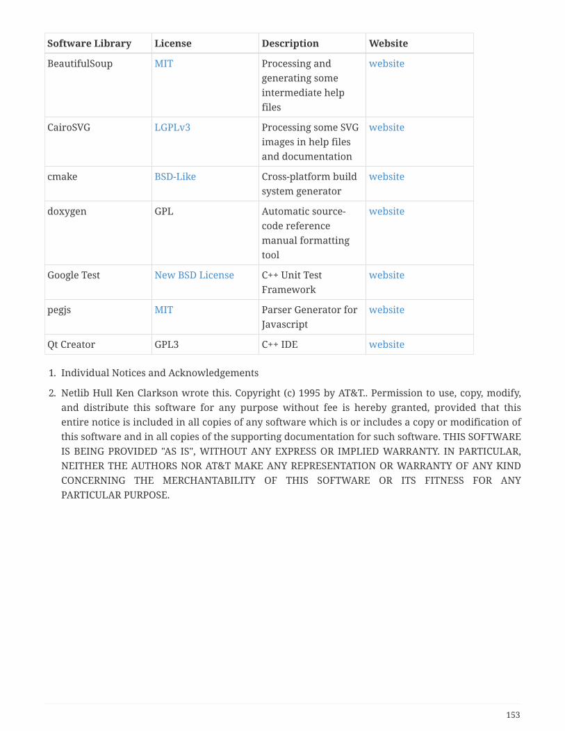
Software Library License Description Website

BeautifulSoup MIT Processing andgenerating someintermediate helpfiles

website

CairoSVG LGPLv3 Processing some SVGimages in help filesand documentation

website

cmake BSD-Like Cross-platform buildsystem generator

website

doxygen GPL Automatic source-code referencemanual formattingtool

website

Google Test New BSD License C++ Unit TestFramework

website

pegjs MIT Parser Generator forJavascript

website

Qt Creator GPL3 C++ IDE website

1. Individual Notices and Acknowledgements

2. Netlib Hull Ken Clarkson wrote this. Copyright (c) 1995 by AT&T.. Permission to use, copy, modify,and distribute this software for any purpose without fee is hereby granted, provided that thisentire notice is included in all copies of any software which is or includes a copy or modification ofthis software and in all copies of the supporting documentation for such software. THIS SOFTWAREIS BEING PROVIDED "AS IS", WITHOUT ANY EXPRESS OR IMPLIED WARRANTY. IN PARTICULAR,NEITHER THE AUTHORS NOR AT&T MAKE ANY REPRESENTATION OR WARRANTY OF ANY KINDCONCERNING THE MERCHANTABILITY OF THIS SOFTWARE OR ITS FITNESS FOR ANYPARTICULAR PURPOSE.

153

https://bazaar.launchpad.net/~leonardr/beautifulsoup/bs4/view/head:/LICENSE

https://www.crummy.com/software/BeautifulSoup/

https://github.com/Kozea/CairoSVG/blob/master/LICENSE

https://cairosvg.org/

http://www.cmake.org/cmake/project/license.html

http://www.cmake.org/

https://www.doxygen.nl/index.html

http://opensource.org/licenses/BSD-3-Clause

https://code.google.com/p/googletest/

https://github.com/pegjs/pegjs/blob/master/LICENSE

https://pegjs.org/

https://qt-project.org/

user manual for retort, pfss and the gemsif computational

Documents