user guide for elekta brachytherapy ace algorithm...
TRANSCRIPT
User Guide for ACE Testing (version 26 April 2016)
1
User Guide for Elekta Brachytherapy ACE Algorithm Testing
Contents
I Introduction
II Test Case Import
A. Accessing the Test Case Repository
B. Downloading the Test Cases
C. Importing a Test Case into OCB a. Importing ACE Images, Plan, Structure Set & Dose Data b. Importing MCNP6 Plan & Dose Data
III Dose Calculation
A. Process Overview
B. Test Case 1 a. Selecting the Plan & Setting the Virtual Source b. Setting the Source Dwell Time c. Setting the Dose Calculation Accuracy & Performing the Calculation d. Creating a 3D Dose Distribution
C. Test Case 2 a. Selecting the Plan & Setting the Virtual Source b. Setting the Source Dwell Time c. Setting the Dose Calculation Accuracy & Performing the Calculation d. Creating a 3D Dose Distribution
D. Test Case 3 a. Selecting the Plan & Setting the Virtual Source b. Setting the Source Dwell Time c. Setting the Dose Calculation Accuracy & Performing the Calculation d. Creating a 3D Dose Distribution
E. Test Case 4 a. Selecting the Plan & Setting the Virtual Source b. Setting the Source Dwell Time c. Setting the Dose Calculation Accuracy & Performing the Calculation d. Creating a 3D Dose Distribution
User Guide for ACE Testing (version 26 April 2016)
2
IV Dose Distribution Comparison
A. Process Overview
B. Doses at Specified Points
C. 2D Dose Maps & 1D Dose Profiles
D. 2D Dose Map Differences
V Test Case Reporting
VI Appendix 1 – Installation of WG Generic Source & Flexitron Afterloader
VII Appendix 2 – MCNP6 Point Dose Values
VIII References
User Guide for ACE Testing (version 26 April 2016)
3
I Introduction
The American Association of Physicists in Medicine (AAPM) Task Group 186 report [1] provides general
guidance for early adopters of model-based dose calculation algorithms (MBDCAs) for brachytherapy
(BT) treatment planning. The report aims to facilitate uniformity of clinical practice, and among its
recommendations is a two-level approach to commissioning MBDCAs embedded in BT treatment
planning systems (TPSs). In commissioning level 1, the clinical physicist needs to assess agreement of
the MBDCA -calculated 3D absolute dose (or dose rate) distribution for a BT source in water medium
with the corresponding dose (or dose rate) distribution obtained in the TPS using AAPM-recommended
consensus TG-43 dosimetry parameters. In commissioning level 2, the physicist needs to compare
MBDCA-calculated dose distributions for virtual phantoms mimicking clinical scenarios with reference
dose distributions derived independently for the same phantom geometries.
The AAPM Working Group on Dose Calculation Algorithms in Brachytherapy (WG-DCAB) [2] was created
to facilitate implementation of the recommendations for MBDCA commissioning made in the TG-186
report. One of its charges is to develop a small number of prototypical virtual phantoms and
corresponding reference dose distributions for use in level 1 and 2 commissioning of high dose rate
(HDR) Ir-192 BT sources. As these sources can be characterized collectively by virtue of their similar
photon emission properties, the WG-DCAB created a generic HDR Ir-192 virtual source for the express
purpose of MBDCA commissioning [3]. At the present time, the generic Ir-192 source model has been
implemented by two MBDCA-based TPS vendors and thus is available to test the commissioning process
described in the TG-186 report. Four virtual phantoms, designated Test Cases 1 - 4, have also been
created by the WG for commissioning purposes and are briefly described below.
Test cases 1 - 3, which are designed to evaluate the fundamental performance of an MBDCA, are based
on a voxelized computational model of a homogeneous water cube (20.1 cm side) set inside either a
water or an air cube (51.1 cm side), represented as a CT DICOM image series. Both cubes have a
common center located at (x, y, z) = (0, 0, 0) cm and their sides are parallel. The dimensions, in-plane
resolution, and number of images were chosen so that 511×511×511 cubic voxels (1 mm)3 fill the space.
The patient coordinate system origin, as defined in the Image Position Patient (0020, 0032) and Image
Orientation Patient (0020, 0037) DICOM tags, coincides with the cube centers which facilitates
calculations and precludes comparison bias, i.e., the center voxel indices are (255, 255, 255) with the
ordering [0:510]. An odd number of voxels was chosen so that the center of a voxel coincides with the
geometrical center of the phantom. The geometries for Test Cases 1 - 3 are summarized in Table 1.
Table 1: Test case 1 – 3 geometries for MBDC algorithm testing
Test Case
Inner cube material ‘Cube’
Outer cube material ‘BgBOX’
Ir-192 source center location
Ir-192 source orientation
Applicator
1 H2O H2O (0, 0, 0) cm +y none
2 H2O air (0, 0, 0) cm +y none
3 H2O air (7, 0, 0) cm +y none
User Guide for ACE Testing (version 26 April 2016)
4
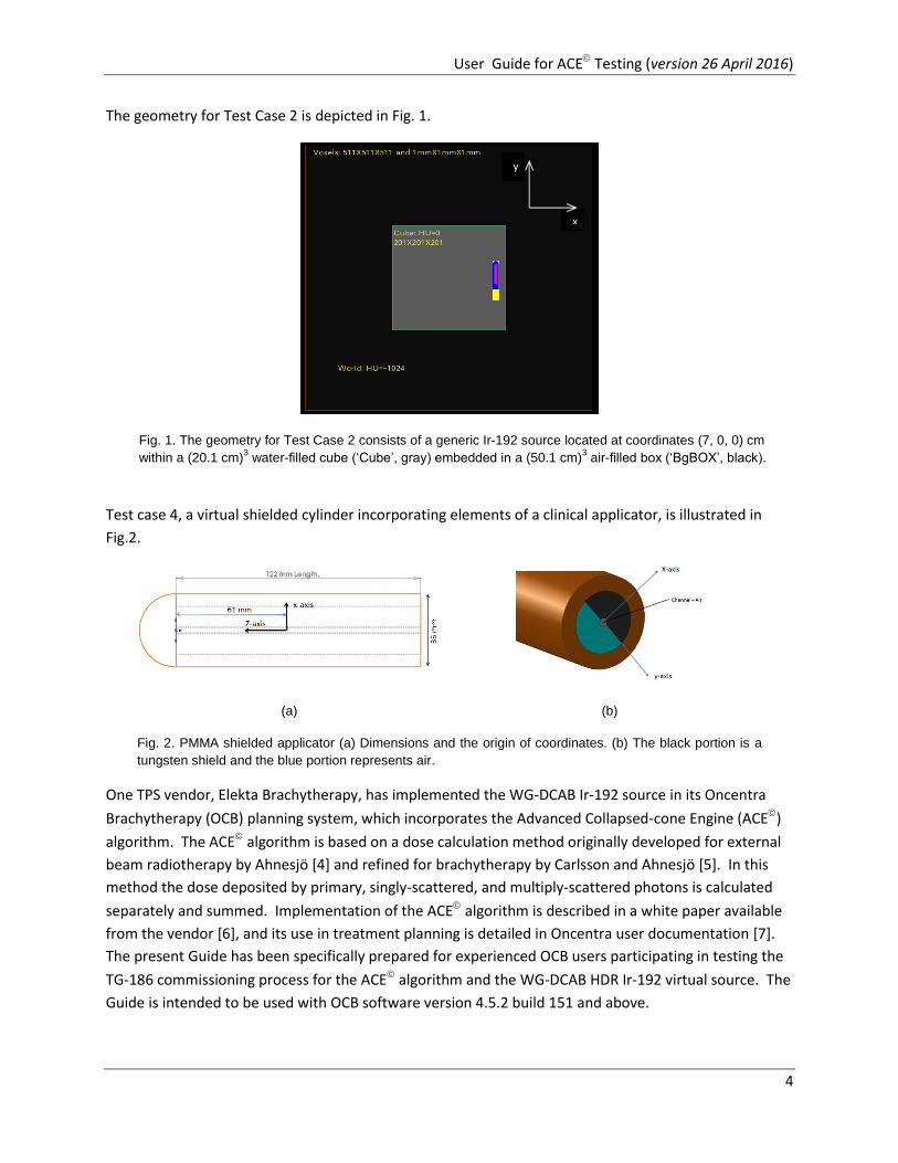
The geometry for Test Case 2 is depicted in Fig. 1.
Fig. 1. The geometry for Test Case 2 consists of a generic Ir-192 source located at coordinates (7, 0, 0) cm
within a (20.1 cm)3 water-filled cube (‘Cube’, gray) embedded in a (50.1 cm)
3 air-filled box (‘BgBOX’, black).
Test case 4, a virtual shielded cylinder incorporating elements of a clinical applicator, is illustrated in
Fig.2.
(a) (b)
Fig. 2. PMMA shielded applicator (a) Dimensions and the origin of coordinates. (b) The black portion is a
tungsten shield and the blue portion represents air.
One TPS vendor, Elekta Brachytherapy, has implemented the WG-DCAB Ir-192 source in its Oncentra
Brachytherapy (OCB) planning system, which incorporates the Advanced Collapsed-cone Engine (ACE)
algorithm. The ACE algorithm is based on a dose calculation method originally developed for external
beam radiotherapy by Ahnesjö [4] and refined for brachytherapy by Carlsson and Ahnesjö [5]. In this
method the dose deposited by primary, singly-scattered, and multiply-scattered photons is calculated
separately and summed. Implementation of the ACE algorithm is described in a white paper available
from the vendor [6], and its use in treatment planning is detailed in Oncentra user documentation [7].
The present Guide has been specifically prepared for experienced OCB users participating in testing the
TG-186 commissioning process for the ACE algorithm and the WG-DCAB HDR Ir-192 virtual source. The
Guide is intended to be used with OCB software version 4.5.2 build 151 and above.
x
y
User Guide for ACE Testing (version 26 April 2016)
5
In overview, the Level 2 commissioning process involves downloading a Test Case treatment plan and an
associated reference dose distribution and importing them into OCB (Sec. II), locally calculating a dose
distribution using ACE (Sec. III), comparing the locally calculated and reference dose distributions (Sec.
IV), and finally reporting the results of the dose comparison (Sec. V). As a “sanity check”, a second
reference dose distribution generated by the WG-DCAB using the ACE algorithm has been made
available in the Test Case repository. Comparison of this latter reference dose distribution with the
locally calculated one should yield dose differences that are practically negligible.
II Test Case Import
In order to perform the Test Case import and dose calculations for commissioning, the WG generic
source and Flexitron afterloader must be available in your OCB system (!). Installation of these items
must occur before performing the set-up and dose calculations steps for a Test Case plan. To install this
afterloader and WG source follow the instructions given in Appendix 1.
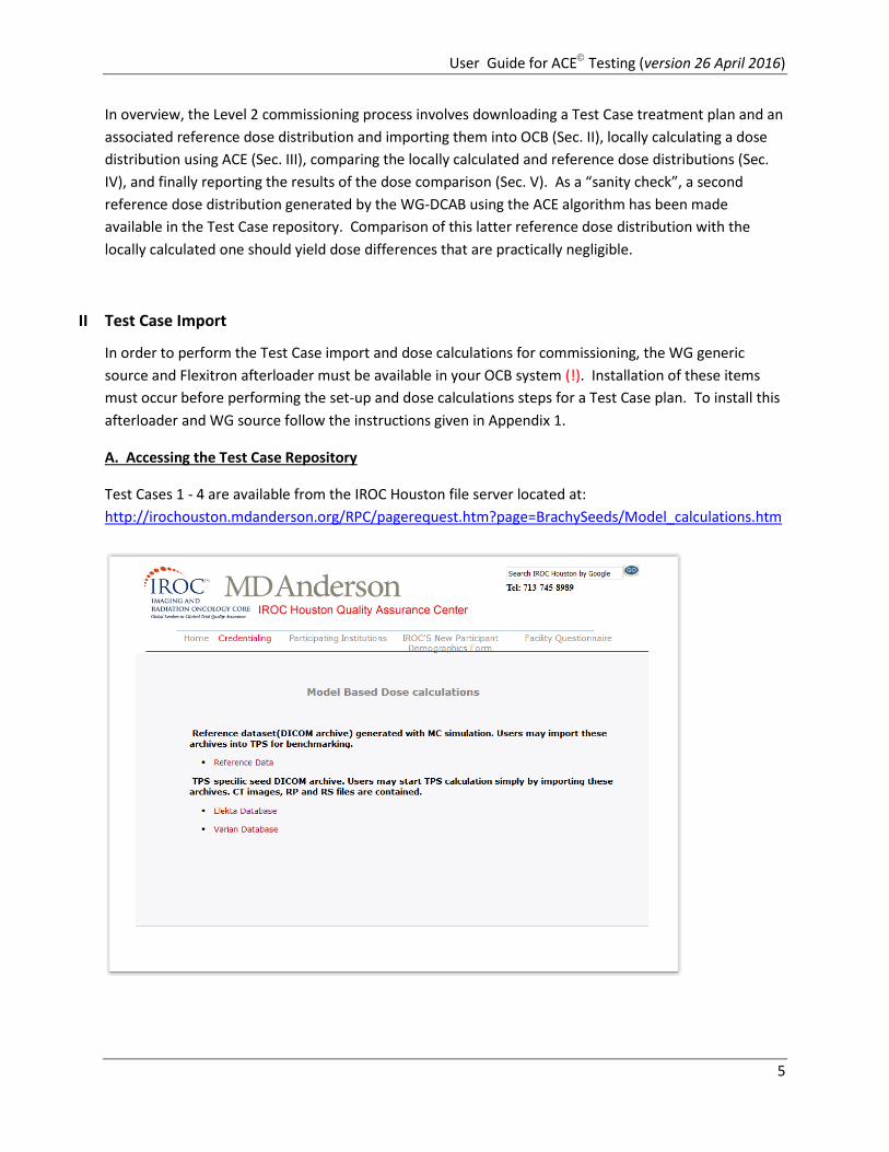
A. Accessing the Test Case Repository
Test Cases 1 - 4 are available from the IROC Houston file server located at:
http://irochouston.mdanderson.org/RPC/pagerequest.htm?page=BrachySeeds/Model_calculations.htm
User Guide for ACE Testing (version 26 April 2016)
6
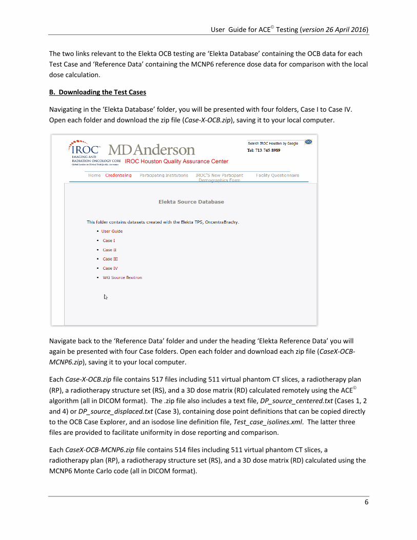
The two links relevant to the Elekta OCB testing are ‘Elekta Database’ containing the OCB data for each
Test Case and ‘Reference Data’ containing the MCNP6 reference dose data for comparison with the local
dose calculation.
B. Downloading the Test Cases
Navigating in the ‘Elekta Database’ folder, you will be presented with four folders, Case I to Case IV.
Open each folder and download the zip file (Case-X-OCB.zip), saving it to your local computer.
Navigate back to the ‘Reference Data’ folder and under the heading ‘Elekta Reference Data’ you will
again be presented with four Case folders. Open each folder and download each zip file (CaseX-OCB-
MCNP6.zip), saving it to your local computer.
Each Case-X-OCB.zip file contains 517 files including 511 virtual phantom CT slices, a radiotherapy plan
(RP), a radiotherapy structure set (RS), and a 3D dose matrix (RD) calculated remotely using the ACE
algorithm (all in DICOM format). The .zip file also includes a text file, DP_source_centered.txt (Cases 1, 2
and 4) or DP_source_displaced.txt (Case 3), containing dose point definitions that can be copied directly
to the OCB Case Explorer, and an isodose line definition file, Test_case_isolines.xml. The latter three
files are provided to facilitate uniformity in dose reporting and comparison.
Each CaseX-OCB-MCNP6.zip file contains 514 files including 511 virtual phantom CT slices, a
radiotherapy plan (RP), a radiotherapy structure set (RS), and a 3D dose matrix (RD) calculated using the
MCNP6 Monte Carlo code (all in DICOM format).

User Guide for ACE Testing (version 26 April 2016)
7
Extract all files from each Case .zip folder to a corresponding local folder on the OCB workstation.
It is suggested that the following directory structure is used:
..\DICOMIMPORTDATA\Case 1\Case-1-OCB\
…………\Case_1_MCNP6\
..\DICOMIMPORTDATA\Case 2\Case-2-OCB\
…………\Case_2_MCNP6\
..\DICOMIMPORTDATA\Case 3\Case-3-OCB\
…………\Case_3_MCNP6\
..\DICOMIMPORTDATA\Case 4\Case-4-OCB\
…………\Case_4_MCNP6\
C. Importing a Test Case into OCB
Note: The following steps use Test Case 1 to illustrate the case import process. The same import process
is used for all test cases.
The import of the Test Case will occur in two steps, firstly importing the pre-calculated ACE plan & dose
and then importing the reference MCNP6 plan & dose.
a. Importing ACE Images, Plan, Structure Set & Dose Data
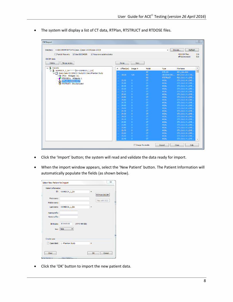
Click on the Import Activity button.
Click the ‘Browse..’ button and select the folder containing the unzipped Test Case,
‘...\Case 1\Case-1-OCB\Case-1-OCB\’
User Guide for ACE Testing (version 26 April 2016)
8
The system will display a list of CT data, RTPlan, RTSTRUCT and RTDOSE files.
Click the ‘Import’ button; the system will read and validate the data ready for import.
When the import window appears, select the ‘New Patient’ button. The Patient Information will
automatically populate the fields (as shown below).
Click the ‘OK’ button to import the new patient data.
User Guide for ACE Testing (version 26 April 2016)
9
A ‘Successful Import’ message will appear when the import is complete. Uncheck the ‘Open
Case’ box and click OK.
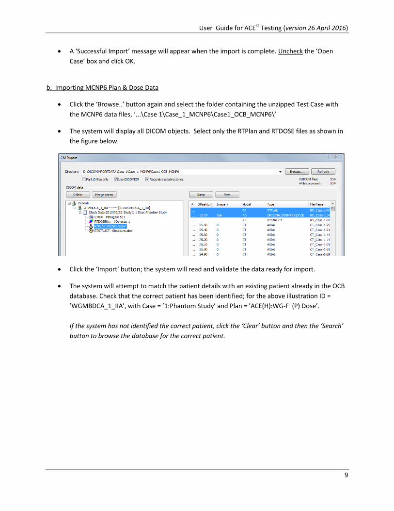
b. Importing MCNP6 Plan & Dose Data
Click the ‘Browse..’ button again and select the folder containing the unzipped Test Case with
the MCNP6 data files, ‘...\Case 1\Case_1_MCNP6\Case1_OCB_MCNP6\’
The system will display all DICOM objects. Select only the RTPlan and RTDOSE files as shown in
the figure below.
Click the ‘Import’ button; the system will read and validate the data ready for import.
The system will attempt to match the patient details with an existing patient already in the OCB
database. Check that the correct patient has been identified; for the above illustration ID =
’WGMBDCA_1_IIA’, with Case = ’1:Phantom Study’ and Plan = ’ACE(H):WG-F (P) Dose’.
If the system has not identified the correct patient, click the ‘Clear’ button and then the ‘Search’
button to browse the database for the correct patient.
User Guide for ACE Testing (version 26 April 2016)
10
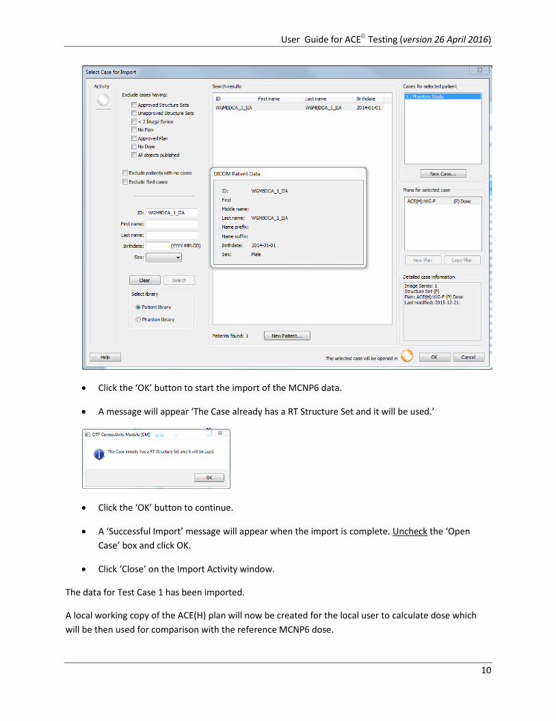
Click the ‘OK’ button to start the import of the MCNP6 data.
A message will appear ‘The Case already has a RT Structure Set and it will be used.’
Click the ‘OK’ button to continue.
A ‘Successful Import’ message will appear when the import is complete. Uncheck the ‘Open
Case’ box and click OK.
Click ‘Close’ on the Import Activity window.
The data for Test Case 1 has been imported.
A local working copy of the ACE(H) plan will now be created for the local user to calculate dose which
will be then used for comparison with the reference MCNP6 dose.
User Guide for ACE Testing (version 26 April 2016)
11
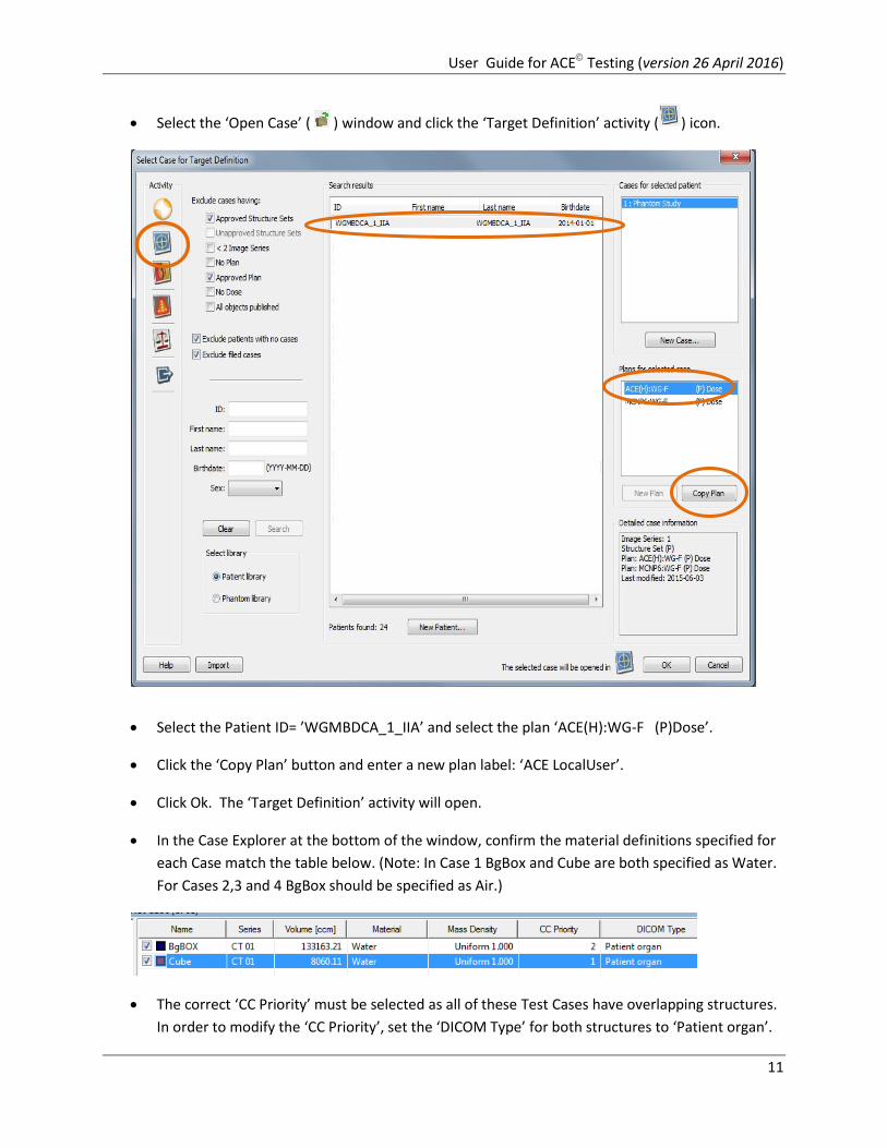
Select the ‘Open Case’ ( ) window and click the ‘Target Definition’ activity ( ) icon.
Select the Patient ID= ’WGMBDCA_1_IIA’ and select the plan ‘ACE(H):WG-F (P)Dose’.
Click the ‘Copy Plan’ button and enter a new plan label: ‘ACE LocalUser’.
Click Ok. The ‘Target Definition’ activity will open.
In the Case Explorer at the bottom of the window, confirm the material definitions specified for
each Case match the table below. (Note: In Case 1 BgBox and Cube are both specified as Water.
For Cases 2,3 and 4 BgBox should be specified as Air.)
The correct ‘CC Priority’ must be selected as all of these Test Cases have overlapping structures.
In order to modify the ‘CC Priority’, set the ‘DICOM Type’ for both structures to ‘Patient organ’.
User Guide for ACE Testing (version 26 April 2016)
12
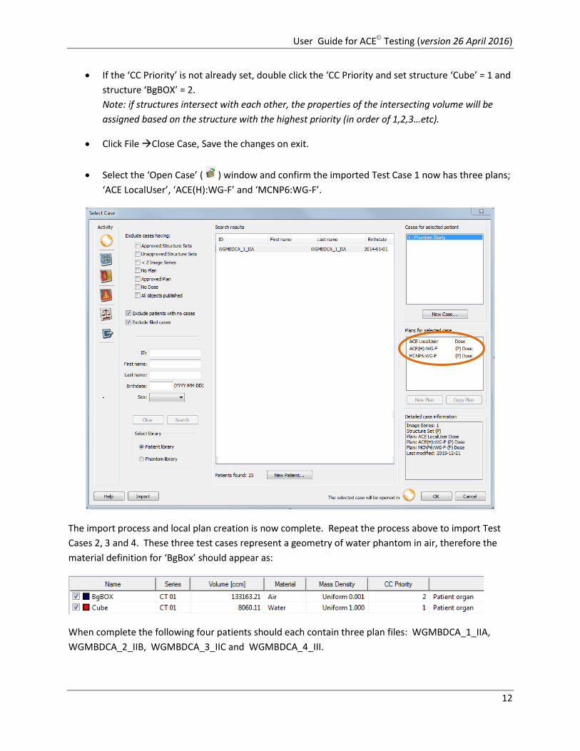
If the ‘CC Priority’ is not already set, double click the ‘CC Priority and set structure ‘Cube’ = 1 and
structure ‘BgBOX’ = 2.
Note: if structures intersect with each other, the properties of the intersecting volume will be
assigned based on the structure with the highest priority (in order of 1,2,3…etc).
Click File Close Case, Save the changes on exit.
Select the ‘Open Case’ ( ) window and confirm the imported Test Case 1 now has three plans;
‘ACE LocalUser’, ‘ACE(H):WG-F’ and ‘MCNP6:WG-F’.
The import process and local plan creation is now complete. Repeat the process above to import Test
Cases 2, 3 and 4. These three test cases represent a geometry of water phantom in air, therefore the
material definition for ‘BgBox’ should appear as:
When complete the following four patients should each contain three plan files: WGMBDCA_1_IIA,
WGMBDCA_2_IIB, WGMBDCA_3_IIC and WGMBDCA_4_III.
User Guide for ACE Testing (version 26 April 2016)
13
III Dose Calculation
A. Process Overview
Level 2 MBDCA commissioning involves comparing a TPS calculated dose distribution with a reference
one, both distributions ideally having been obtained for the same value of total reference air kerma
(TRAK) emitted by the radiation source. TRAK can be expressed as a product of the source air kerma
rate constant [µGy·m2·h-1·MBq-1], source activity [MBq], source total dwell time [s], and a units
conversion factor (3.6 108)-1 [Gy·µGy-1 h·s-1]. The air kerma rate constant for the generic Ir-192 WG
source is 0.098 [µGy·m2·h-1·MBq-1] [3]; for purposes of MBDCA commissioning, the source activity has
been specified as 3.7 105 MBq (10.0 Ci). Accordingly, preparing for local dose calculation requires that
you manually set a single dwell time for a single dwell position for each Test Case. In this manner the
TRAK is fixed to the same value used to normalize the corresponding reference dose distribution,
enabling direct comparison of the locally calculated and reference dose distributions.
B. Test Case 1
a. Selecting the Plan & Setting the Virtual Source
Select the Brachy Planning activity , then select patient ‘WGMBDCA_1_IIA’ and plan ‘ACE
LocalUser’, and click the ‘OK’ button.
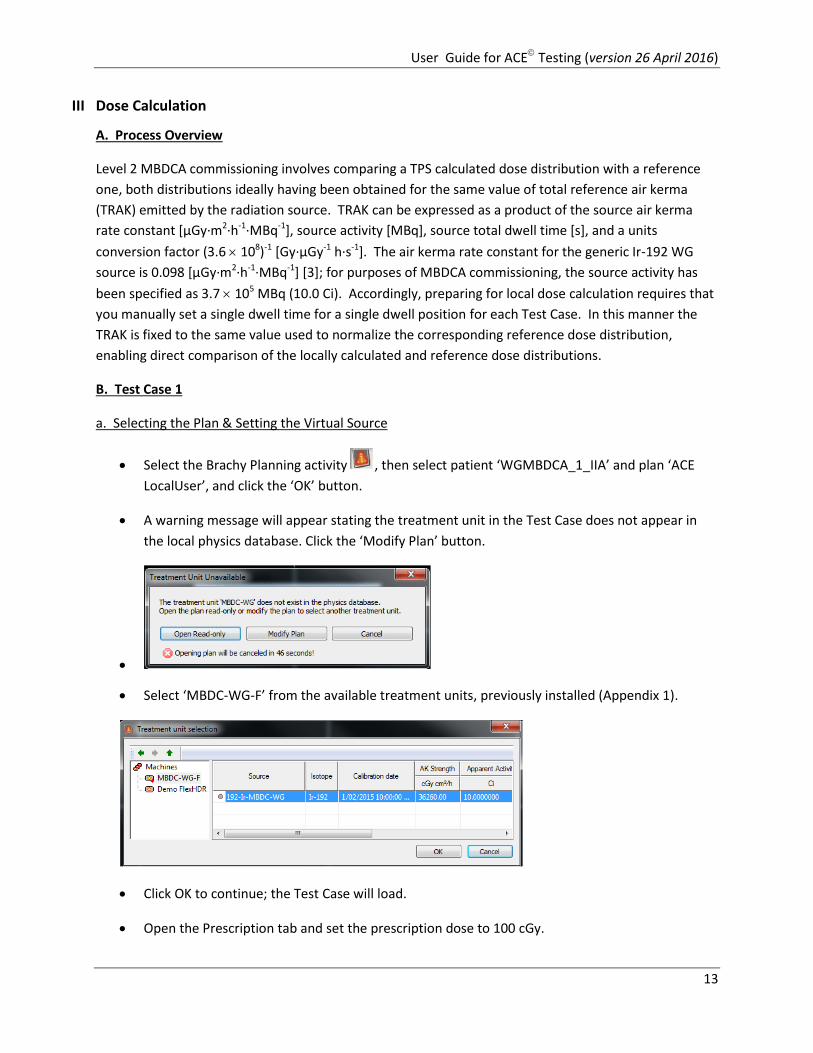
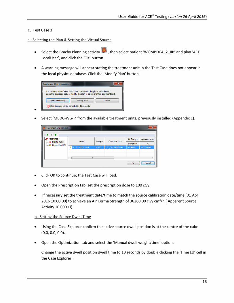
A warning message will appear stating the treatment unit in the Test Case does not appear in
the local physics database. Click the ‘Modify Plan’ button.
Select ‘MBDC-WG-F’ from the available treatment units, previously installed (Appendix 1).
Click OK to continue; the Test Case will load.
Open the Prescription tab and set the prescription dose to 100 cGy.
User Guide for ACE Testing (version 26 April 2016)
14
If necessary set the treatment date/time to match the source calibration date/time (01 Apr 2016
10:00:00) to achieve an Air Kerma Strength of 36260.00 cGy cm2/h ( Apparent Source Activity
10.000 Ci)
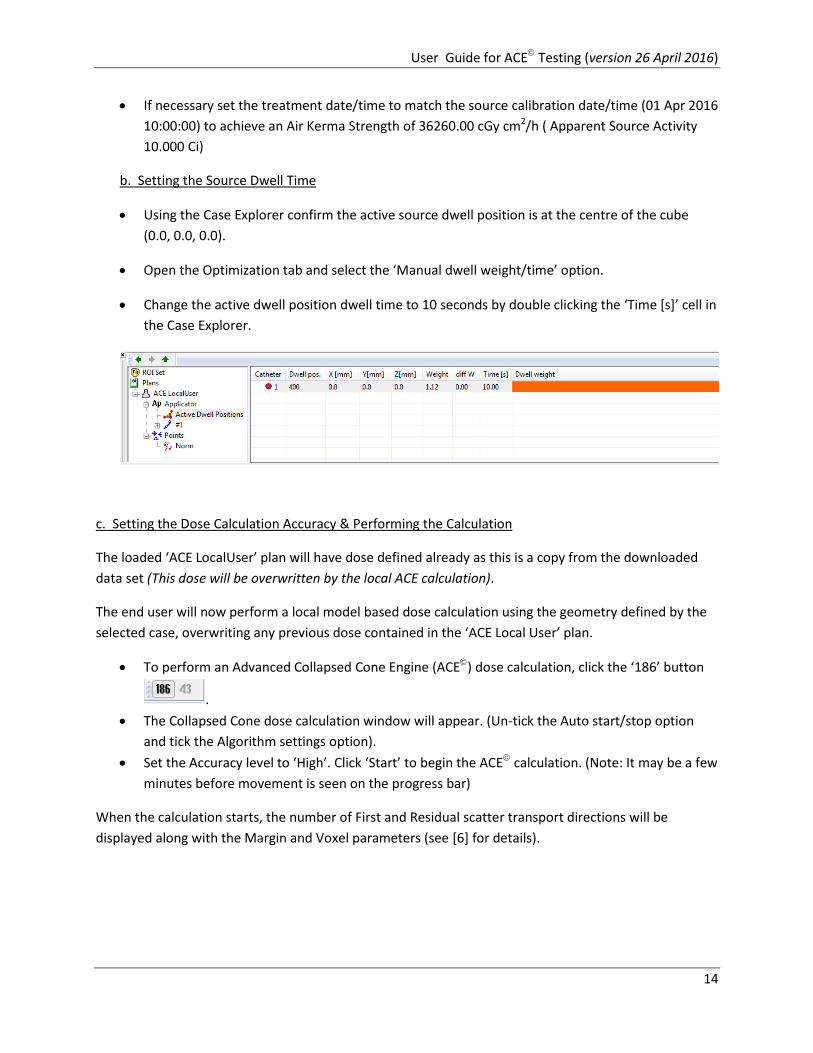
b. Setting the Source Dwell Time
Using the Case Explorer confirm the active source dwell position is at the centre of the cube
(0.0, 0.0, 0.0).
Open the Optimization tab and select the ‘Manual dwell weight/time’ option.
Change the active dwell position dwell time to 10 seconds by double clicking the ‘Time [s]’ cell in
the Case Explorer.
c. Setting the Dose Calculation Accuracy & Performing the Calculation
The loaded ‘ACE LocalUser’ plan will have dose defined already as this is a copy from the downloaded
data set (This dose will be overwritten by the local ACE calculation).
The end user will now perform a local model based dose calculation using the geometry defined by the
selected case, overwriting any previous dose contained in the ‘ACE Local User’ plan.
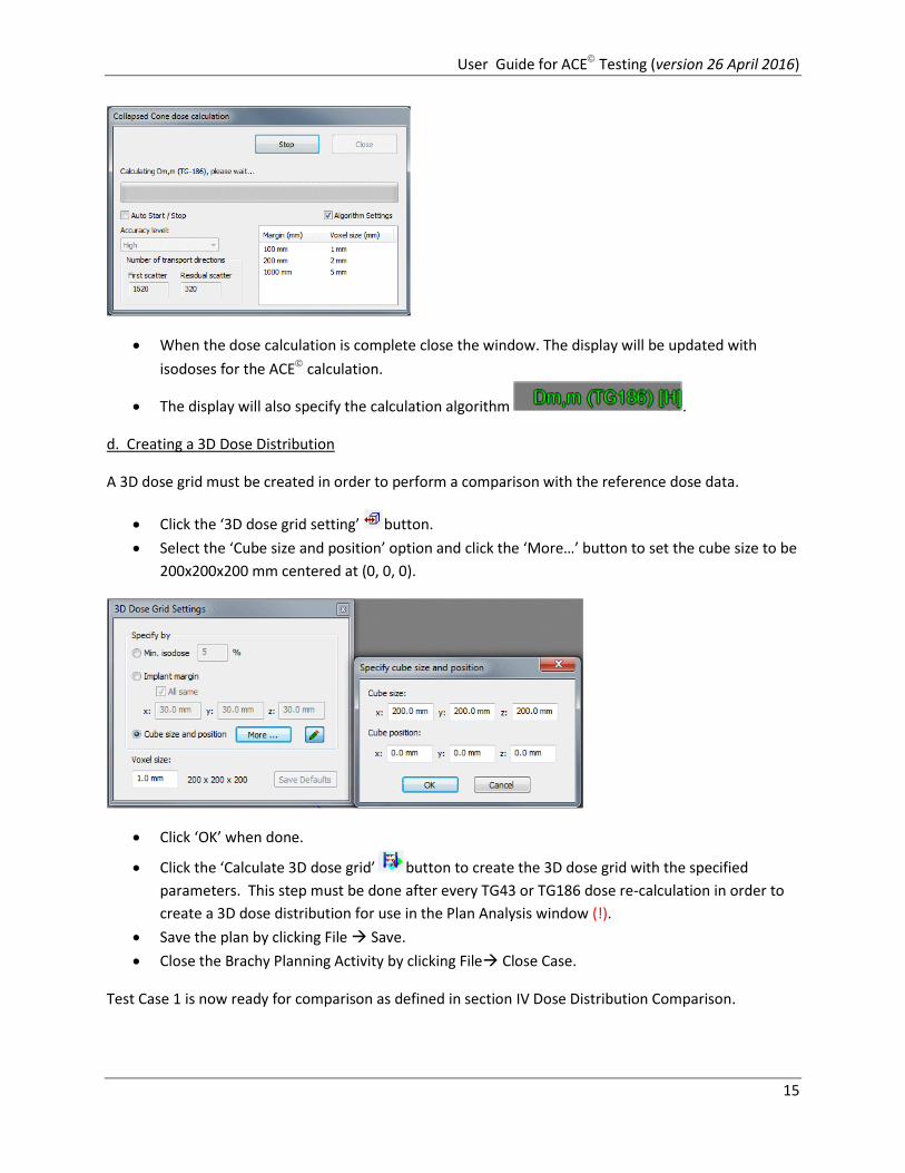
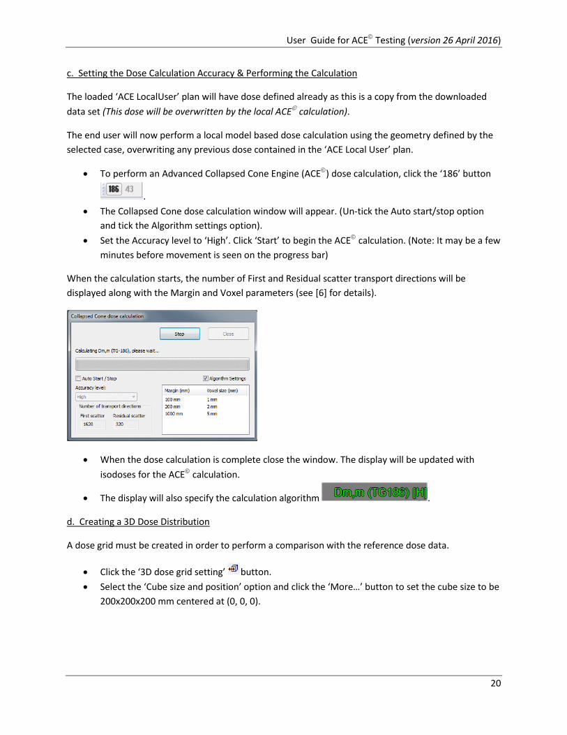
To perform an Advanced Collapsed Cone Engine (ACE) dose calculation, click the ‘186’ button
.
The Collapsed Cone dose calculation window will appear. (Un-tick the Auto start/stop option
and tick the Algorithm settings option).
Set the Accuracy level to ‘High’. Click ‘Start’ to begin the ACE calculation. (Note: It may be a few
minutes before movement is seen on the progress bar)
When the calculation starts, the number of First and Residual scatter transport directions will be
displayed along with the Margin and Voxel parameters (see [6] for details).
User Guide for ACE Testing (version 26 April 2016)
15
When the dose calculation is complete close the window. The display will be updated with
isodoses for the ACE calculation.
The display will also specify the calculation algorithm .
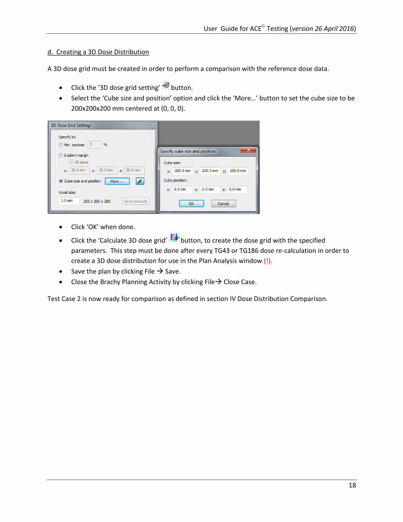
d. Creating a 3D Dose Distribution
A 3D dose grid must be created in order to perform a comparison with the reference dose data.
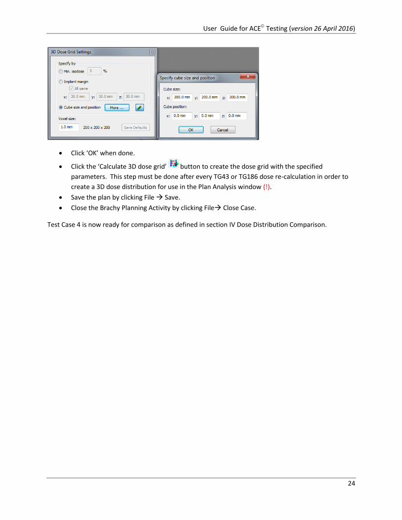
Click the ‘3D dose grid setting’ button.
Select the ‘Cube size and position’ option and click the ‘More…’ button to set the cube size to be
200x200x200 mm centered at (0, 0, 0).
Click ‘OK’ when done.
Click the ‘Calculate 3D dose grid’ button to create the 3D dose grid with the specified
parameters. This step must be done after every TG43 or TG186 dose re-calculation in order to
create a 3D dose distribution for use in the Plan Analysis window (!).
Save the plan by clicking File Save.
Close the Brachy Planning Activity by clicking File Close Case.
Test Case 1 is now ready for comparison as defined in section IV Dose Distribution Comparison.
User Guide for ACE Testing (version 26 April 2016)
16
C. Test Case 2
a. Selecting the Plan & Setting the Virtual Source
Select the Brachy Planning activity , then select patient ‘WGMBDCA_2_IIB’ and plan ‘ACE
LocalUser’, and click the ‘OK’ button. .
A warning message will appear stating the treatment unit in the Test Case does not appear in
the local physics database. Click the ‘Modify Plan’ button.
Select ‘MBDC-WG-F’ from the available treatment units, previously installed (Appendix 1).
Click OK to continue; the Test Case will load.
Open the Prescription tab, set the prescription dose to 100 cGy.
If necessary set the treatment date/time to match the source calibration date/time (01 Apr
2016 10:00:00) to achieve an Air Kerma Strength of 36260.00 cGy cm2/h ( Apparent Source
Activity 10.000 Ci)
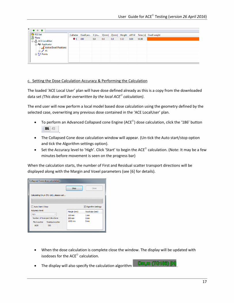
b. Setting the Source Dwell Time
Using the Case Explorer confirm the active source dwell position is at the centre of the cube
(0.0, 0.0, 0.0).
Open the Optimization tab and select the ‘Manual dwell weight/time’ option.
Change the active dwell position dwell time to 10 seconds by double clicking the ‘Time [s]’ cell in
the Case Explorer.
User Guide for ACE Testing (version 26 April 2016)
17
c. Setting the Dose Calculation Accuracy & Performing the Calculation
The loaded ‘ACE Local User’ plan will have dose defined already as this is a copy from the downloaded
data set (This dose will be overwritten by the local ACE calculation).
The end user will now perform a local model based dose calculation using the geometry defined by the
selected case, overwriting any previous dose contained in the ‘ACE LocalUser’ plan.
To perform an Advanced Collapsed cone Engine (ACE) dose calculation, click the ‘186’ button
.
The Collapsed Cone dose calculation window will appear. (Un-tick the Auto start/stop option
and tick the Algorithm settings option).
Set the Accuracy level to ‘High’. Click ‘Start’ to begin the ACE calculation. (Note: It may be a few
minutes before movement is seen on the progress bar)
When the calculation starts, the number of First and Residual scatter transport directions will be
displayed along with the Margin and Voxel parameters (see [6] for details).
When the dose calculation is complete close the window. The display will be updated with
isodoses for the ACE calculation.
The display will also specify the calculation algorithm .
User Guide for ACE Testing (version 26 April 2016)
18
d. Creating a 3D Dose Distribution
A 3D dose grid must be created in order to perform a comparison with the reference dose data.
Click the ‘3D dose grid setting’ button.
Select the ‘Cube size and position’ option and click the ‘More…’ button to set the cube size to be
200x200x200 mm centered at (0, 0, 0).
Click ‘OK’ when done.
Click the ‘Calculate 3D dose grid’ button, to create the dose grid with the specified
parameters. This step must be done after every TG43 or TG186 dose re-calculation in order to
create a 3D dose distribution for use in the Plan Analysis window (!).
Save the plan by clicking File Save.
Close the Brachy Planning Activity by clicking File Close Case.
Test Case 2 is now ready for comparison as defined in section IV Dose Distribution Comparison.
User Guide for ACE Testing (version 26 April 2016)
19
D. Test Case 3
a. Selecting the Plan & Setting the Virtual Source
Select the Brachy Planning activity , then select patient ‘WGMBDCA_3_IIC’ and plan ‘ACE
LocalUser’, and click the ‘OK’ button.
A warning message will appear stating the treatment unit in the Test Case does not appear in
the local physics database. Click the ‘Modify Plan’ button.
Select the ‘MBDC-WG-F’ from the available treatment units, previously installed (Appendix 1).
Click OK to continue; the Test Case will load.
Open the Prescription tab, set the prescription dose to 100 cGy.
If necessary set the treatment date/time to match the source calibration date/time (01 Apr 2016
10:00:00) to achieve an Air Kerma Strength of 36260.00 cGy cm2/h ( Apparent Source Activity
10.000 Ci)
b. Setting the Source Dwell Time
Using the Case Explorer confirm the active source dwell position is offset from the centre of the
cube
(70.0, 0.0, 0.0).
Open the Optimization tab and select the ‘Manual dwell weight/time’ option.
Change the active dwell position dwell time to 10 seconds by double clicking the ‘Time [s]’ cell in
the Case Explorer.
User Guide for ACE Testing (version 26 April 2016)
20
c. Setting the Dose Calculation Accuracy & Performing the Calculation
The loaded ‘ACE LocalUser’ plan will have dose defined already as this is a copy from the downloaded
data set (This dose will be overwritten by the local ACE calculation).
The end user will now perform a local model based dose calculation using the geometry defined by the
selected case, overwriting any previous dose contained in the ‘ACE Local User’ plan.
To perform an Advanced Collapsed Cone Engine (ACE) dose calculation, click the ‘186’ button
.
The Collapsed Cone dose calculation window will appear. (Un-tick the Auto start/stop option
and tick the Algorithm settings option).
Set the Accuracy level to ‘High’. Click ‘Start’ to begin the ACE calculation. (Note: It may be a few
minutes before movement is seen on the progress bar)
When the calculation starts, the number of First and Residual scatter transport directions will be
displayed along with the Margin and Voxel parameters (see [6] for details).
When the dose calculation is complete close the window. The display will be updated with
isodoses for the ACE calculation.
The display will also specify the calculation algorithm .
d. Creating a 3D Dose Distribution
A dose grid must be created in order to perform a comparison with the reference dose data.
Click the ‘3D dose grid setting’ button.
Select the ‘Cube size and position’ option and click the ‘More…’ button to set the cube size to be
200x200x200 mm centered at (0, 0, 0).

User Guide for ACE Testing (version 26 April 2016)
21
Click ‘OK’ when done.
Click the ‘Calculate 3D dose grid’ button to create the dose grid with the specified
parameters. This step must be done after every TG43 or TG186 dose re-calculation in order to
create a 3D dose distribution for use in the Plan Analysis window (!).
Save the plan by clicking File Save.
Close the Brachy Planning Activity by clicking File Close Case.
Test Case 3 is now ready for comparison as defined in section IV Dose Distribution Comparison.
User Guide for ACE Testing (version 26 April 2016)
22
E. Test Case 4
An Applicator Modelling license is required to perform the set-up and calculations for Test Case 4. The
user should confirm that Applicator Modelling is installed on their OCB system prior to working through
Test Case 4.
a. Selecting the Plan & Setting the Virtual Source
Select the Brachy Planning activity , then select patient ‘WGMBDCA_4_III’ and plan ‘ACE
LocalUser’, and click the ‘OK’ button.
A warning message will appear stating the treatment unit in the Test Case does not appear in
the local physics database. Click the ‘Modify Plan’ button.
Select the ‘MBDC-WG-F’ from the available treatment units, previously installed (Appendix 1).
Click OK to continue; the Test Case will load.
Open the Prescription tab, set the prescription dose to 100 cGy.
If necessary set the treatment date/time to match the source calibration date/time (01 Apr 2016
10:00:00) to achieve an Air Kerma Strength of 36260.00 cGy cm2/h ( Apparent Source Activity
10.000 Ci)
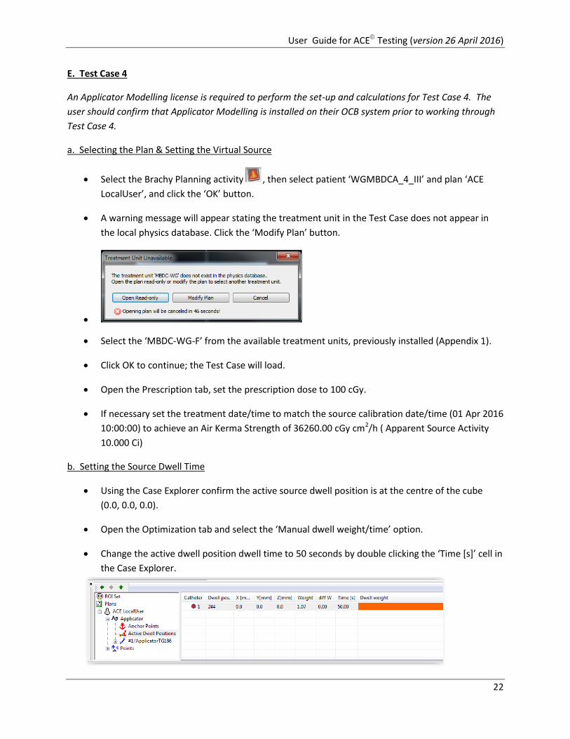
b. Setting the Source Dwell Time
Using the Case Explorer confirm the active source dwell position is at the centre of the cube
(0.0, 0.0, 0.0).
Open the Optimization tab and select the ‘Manual dwell weight/time’ option.
Change the active dwell position dwell time to 50 seconds by double clicking the ‘Time [s]’ cell in
the Case Explorer.

User Guide for ACE Testing (version 26 April 2016)
23
c. Setting the Dose Calculation Accuracy & Performing the Calculation
The loaded ‘ACE LocalUser’ plan will have dose defined already as this is a copy from the downloaded
data set (This dose will be overwritten by the local ACE calculation).
The end user will now perform a local model based dose calculation using the geometry defined by the
selected case, overwriting any previous dose contained in the ‘ACE Local User’ plan.
To perform an Advanced Collapsed Cone Engine (ACE) dose calculation, click the ‘186’ button
.
The Collapsed Cone dose calculation window will appear. (Un-tick the Auto start/stop option
and tick the Algorithm settings option).
Set the Accuracy level to ‘High’. Click ‘Start’ to begin the ACE calculation. (Note: It may be a few
minutes before movement is seen on the progress bar)
When the calculation starts, the number of First and Residual scatter transport directions will be
displayed along with the Margin and Voxel parameters (see [6] for details).
When the dose calculation is complete close the window. The display will be updated with
isodoses for the ACE calculation.
The display will also specify the calculation algorithm .
d. Creating a 3D Dose Distribution
A dose grid must be created in order to perform a comparison with the reference dose data.
Click the ‘3D dose grid setting’ button.
Select the ‘Cube size and position’ option and click the ‘More…’ button to set the cube size to be
200x200x200 mm centered at (0, 0, 0).
User Guide for ACE Testing (version 26 April 2016)
24
Click ‘OK’ when done.
Click the ‘Calculate 3D dose grid’ button to create the dose grid with the specified
parameters. This step must be done after every TG43 or TG186 dose re-calculation in order to
create a 3D dose distribution for use in the Plan Analysis window (!).
Save the plan by clicking File Save.
Close the Brachy Planning Activity by clicking File Close Case.
Test Case 4 is now ready for comparison as defined in section IV Dose Distribution Comparison.
User Guide for ACE Testing (version 26 April 2016)
25
IV Dose Distribution Comparison
A. Process Overview
The comparison of 3D dose distributions is typically done at specified points, in selected planes (dose
maps), or for defined volumes within the distributions. Commonly used comparative metrics include
dose differences, dose ratios, and the gamma index [8]. The comparison tools available within the OCB
treatment planning system are limited to those based solely on dose differences; correspondingly, the
detailed dose comparison and reporting guidance provided below is restricted to dose differences.
To augment the limited dose comparison tools currently available in OCB, end-users can optionally make
use of third party software of their choice and report their experiences using it. In this regard, public-
domain software such as BrachyGuide v2 [9] (available at: http://www.rdl.gr/downloads ) and SlicerRT
[10] (available at: http://slicerrt.github.io/ ) may be of interest. Note that the use of third party
software for dose comparison within the current context, although encouraged, is not required.
B. Doses at Specified Points
The tab-delimited text file DP_source_centered.txt or DP_source_displaced.txt downloaded from the
Elekta database with the other Test Case data defines two sets of six dose points to be used as
comparison standards. For both source positions, the two sets contain points centered on the faces of
cubes of sides 20 mm and 100 mm, respectively; the cubes in turn are centered at the radiation source.
For the source displaced geometry and the large cube, the dose point at (x, y, z) = (120, 0, 0) mm has
been moved to (x, y, z) = (100, 0, 0) mm to keep it within the water-filled part of the phantom.
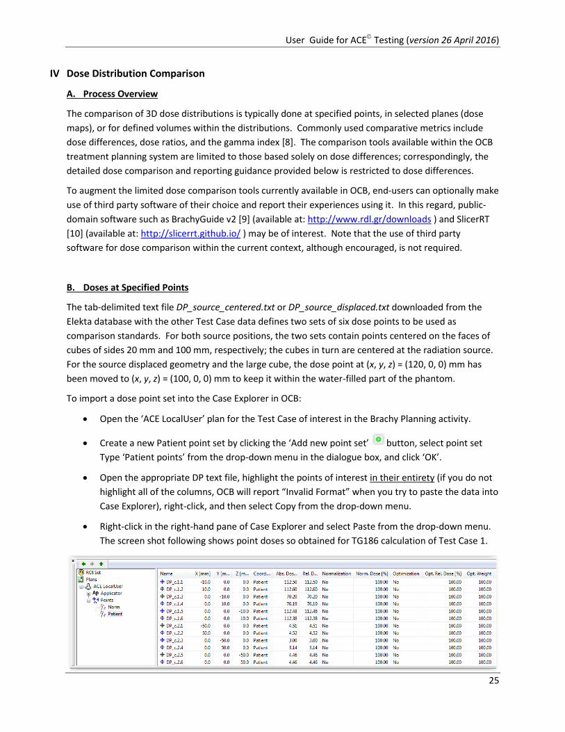
To import a dose point set into the Case Explorer in OCB:
Open the ‘ACE LocalUser’ plan for the Test Case of interest in the Brachy Planning activity.
Create a new Patient point set by clicking the ‘Add new point set’ button, select point set
Type ‘Patient points’ from the drop-down menu in the dialogue box, and click ‘OK’.
Open the appropriate DP text file, highlight the points of interest in their entirety (if you do not
highlight all of the columns, OCB will report “Invalid Format” when you try to paste the data into
Case Explorer), right-click, and then select Copy from the drop-down menu.
Right-click in the right-hand pane of Case Explorer and select Paste from the drop-down menu.
The screen shot following shows point doses so obtained for TG186 calculation of Test Case 1.
User Guide for ACE Testing (version 26 April 2016)
26
To obtain dose values at other points in the phantom that may also be of interest, edit the DP text file to
include the coordinates of these points. Then highlight these additional points in their entirety, right-
click and select ‘Copy’ from the drop-down menu, right-click in the right-hand pane of Case Explorer and
select ‘Paste insert’ from the drop-down menu.
For each Test Case, a summary table of DP text file point dose differences (%) between locally calculated
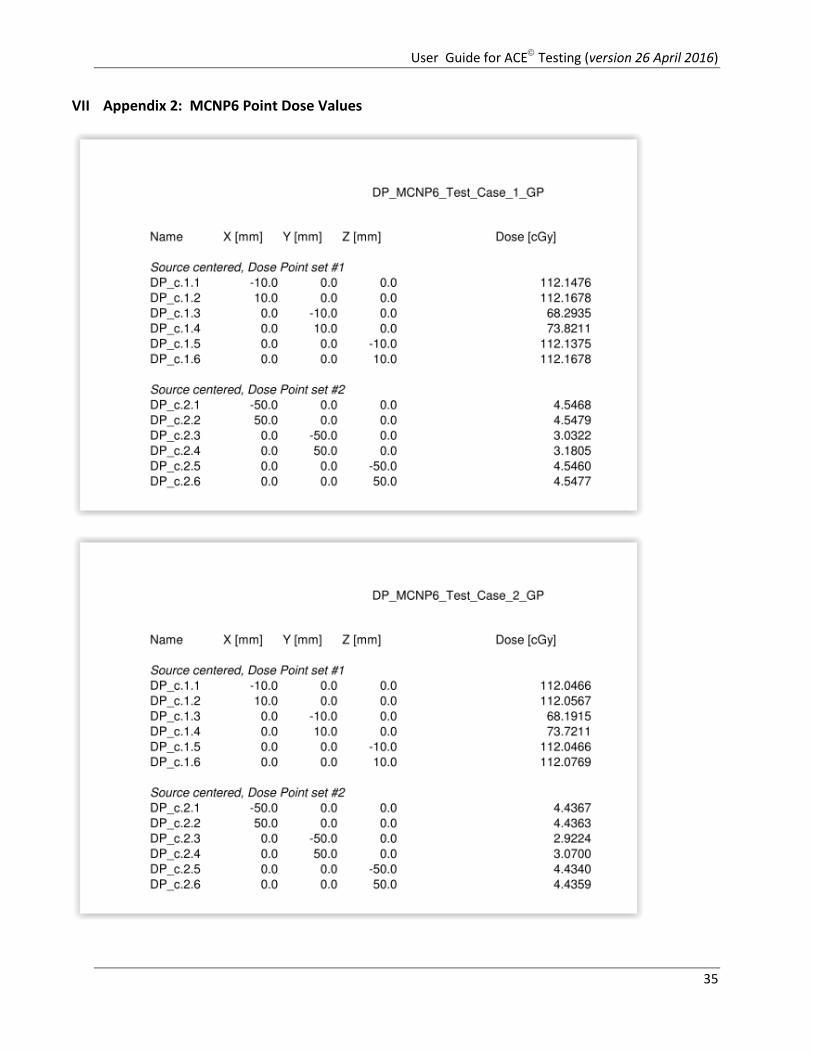
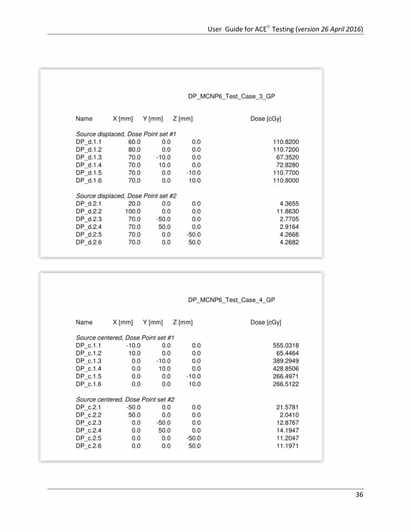
and MCNP6 reference dose values should be compiled and reported. The MCNP6 reference dose values
for each Test Case can be found in Appendix 2.
C. 2D Dose Maps & 1D Dose Profiles
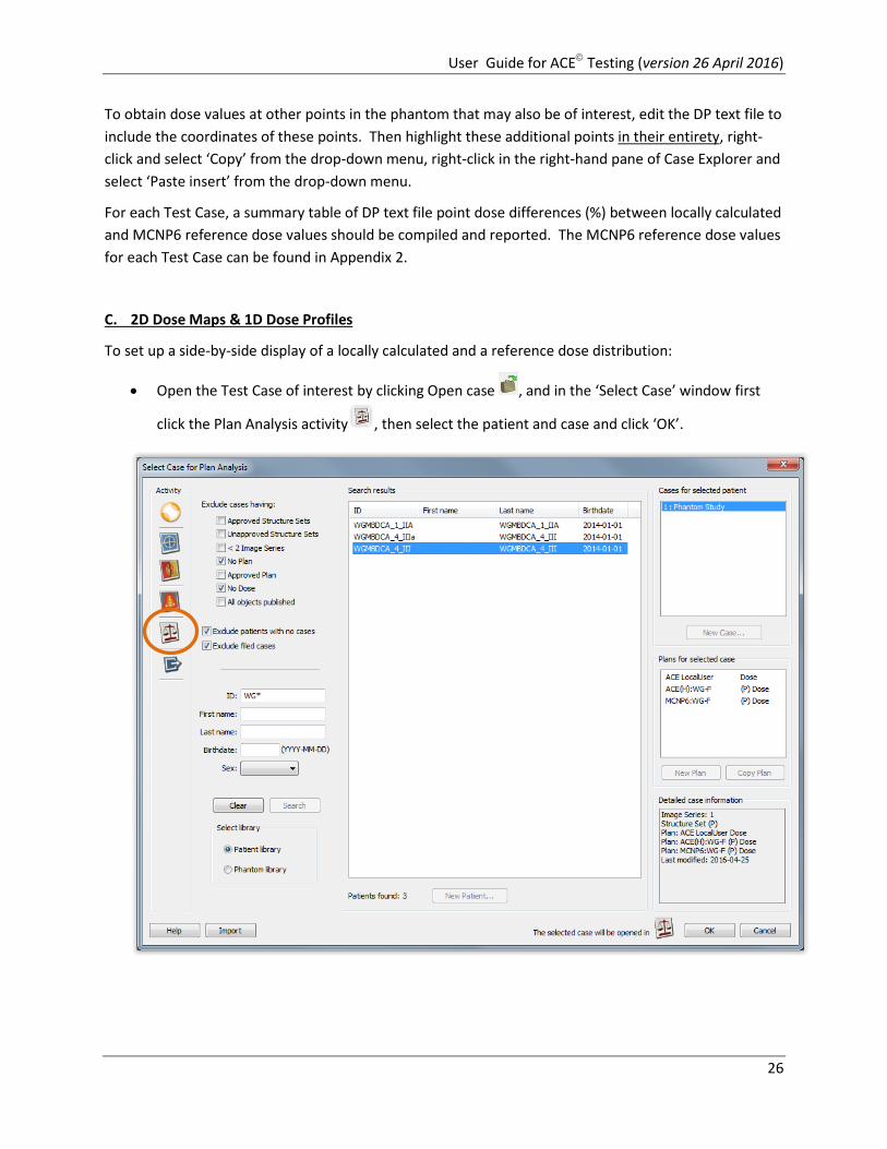
To set up a side-by-side display of a locally calculated and a reference dose distribution:
Open the Test Case of interest by clicking Open case , and in the ‘Select Case’ window first
click the Plan Analysis activity , then select the patient and case and click ‘OK’.
User Guide for ACE Testing (version 26 April 2016)
27
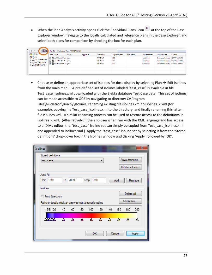
When the Plan Analysis activity opens click the ‘Individual Plans’ icon at the top of the Case
Explorer window, navigate to the locally calculated and reference plans in the Case Explorer, and
select both plans for comparison by checking the box for each plan.
Choose or define an appropriate set of isolines for dose display by selecting Plan Edit Isolines
from the main menu. A pre-defined set of isolines labeled “test_case” is available in file
Test_case_isolines.xml downloaded with the Elekta database Test Case data. This set of isolines
can be made accessible to OCB by navigating to directory C:\Program
Files\Nucletron\Brachy\Isolines, renaming existing file isolines.xml to isolines_x.xml (for
example), copying file Test_case_isolines.xml to the directory, and finally renaming this latter
file isolines.xml. A similar renaming process can be used to restore access to the definitions in
isolines_x.xml. (Alternatively, if the end-user is familiar with the XML language and has access
to an XML editor, the “test_case” isoline set can simply be copied from Test_case_isolines.xml
and appended to isolines.xml.) Apply the “test_case” isoline set by selecting it from the ‘Stored
definitions’ drop-down box in the Isolines window and clicking ‘Apply’ followed by ‘OK’.
User Guide for ACE Testing (version 26 April 2016)
28
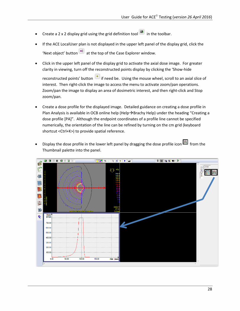
Create a 2 x 2 display grid using the grid definition tool in the toolbar.
If the ACE LocalUser plan is not displayed in the upper left panel of the display grid, click the
‘Next object’ button at the top of the Case Explorer window.
Click in the upper left panel of the display grid to activate the axial dose image. For greater
clarity in viewing, turn off the reconstructed points display by clicking the ‘Show-hide
reconstructed points’ button if need be. Using the mouse wheel, scroll to an axial slice of
interest. Then right-click the image to access the menu to activate zoom/pan operations.
Zoom/pan the image to display an area of dosimetric interest, and then right-click and Stop
zoom/pan.
Create a dose profile for the displayed image. Detailed guidance on creating a dose profile in
Plan Analysis is available in OCB online help (HelpBrachy Help) under the heading “Creating a
dose profile [PA]”. Although the endpoint coordinates of a profile line cannot be specified
numerically, the orientation of the line can be refined by turning on the cm grid (keyboard
shortcut <Ctrl+K>) to provide spatial reference.
Display the dose profile in the lower left panel by dragging the dose profile icon from the
Thumbnail palette into the panel.
User Guide for ACE Testing (version 26 April 2016)
29
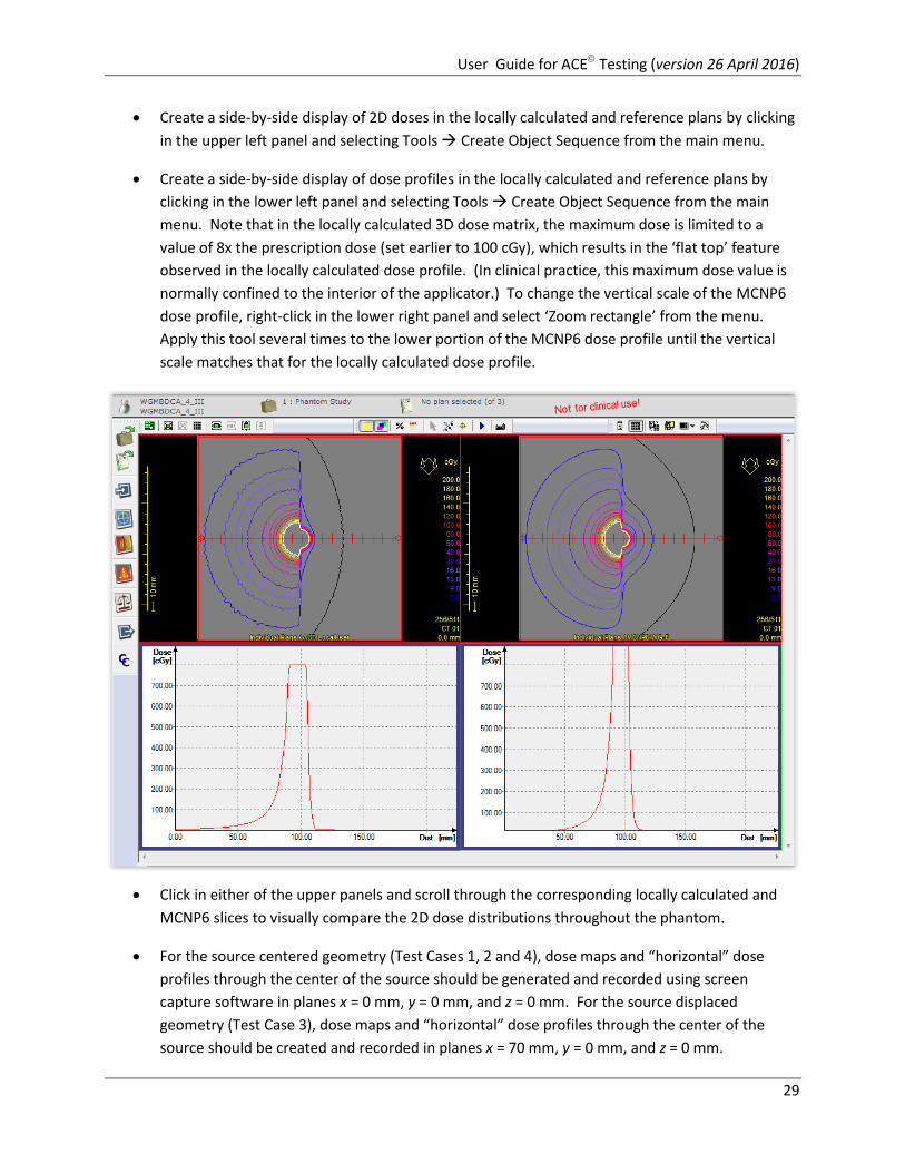
Create a side-by-side display of 2D doses in the locally calculated and reference plans by clicking
in the upper left panel and selecting Tools Create Object Sequence from the main menu.
Create a side-by-side display of dose profiles in the locally calculated and reference plans by
clicking in the lower left panel and selecting Tools Create Object Sequence from the main
menu. Note that in the locally calculated 3D dose matrix, the maximum dose is limited to a
value of 8x the prescription dose (set earlier to 100 cGy), which results in the ‘flat top’ feature
observed in the locally calculated dose profile. (In clinical practice, this maximum dose value is
normally confined to the interior of the applicator.) To change the vertical scale of the MCNP6
dose profile, right-click in the lower right panel and select ‘Zoom rectangle’ from the menu.
Apply this tool several times to the lower portion of the MCNP6 dose profile until the vertical
scale matches that for the locally calculated dose profile.
Click in either of the upper panels and scroll through the corresponding locally calculated and
MCNP6 slices to visually compare the 2D dose distributions throughout the phantom.
For the source centered geometry (Test Cases 1, 2 and 4), dose maps and “horizontal” dose
profiles through the center of the source should be generated and recorded using screen
capture software in planes x = 0 mm, y = 0 mm, and z = 0 mm. For the source displaced
geometry (Test Case 3), dose maps and “horizontal” dose profiles through the center of the
source should be created and recorded in planes x = 70 mm, y = 0 mm, and z = 0 mm.
User Guide for ACE Testing (version 26 April 2016)
30
D. 2D Dose Map Differences
To display differences between a locally calculated and a reference dose distribution:
Open the Test Case of interest by clicking Open case , and in the ‘Select Case’ window first
click the Plan Analysis activity , then select the patient and case and click ‘OK’.
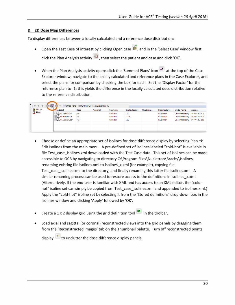
When the Plan Analysis activity opens click the ‘Summed Plans’ icon at the top of the Case
Explorer window, navigate to the locally calculated and reference plans in the Case Explorer, and
select the plans for comparison by checking the box for each. Set the ‘Display Factor’ for the
reference plan to -1; this yields the difference in the locally calculated dose distribution relative
to the reference distribution.
Choose or define an appropriate set of isolines for dose difference display by selecting Plan
Edit Isolines from the main menu. A pre-defined set of isolines labeled “cold-hot” is available in
file Test_case_isolines.xml downloaded with the Test Case data. This set of isolines can be made
accessible to OCB by navigating to directory C:\Program Files\Nucletron\Brachy\Isolines,
renaming existing file isolines.xml to isolines_x.xml (for example), copying file
Test_case_isolines.xml to the directory, and finally renaming this latter file isolines.xml. A
similar renaming process can be used to restore access to the definitions in isolines_x.xml.
(Alternatively, if the end-user is familiar with XML and has access to an XML editor, the “cold-
hot” isoline set can simply be copied from Test_case_isolines.xml and appended to isolines.xml.)
Apply the “cold-hot” isoline set by selecting it from the ‘Stored definitions’ drop-down box in the
Isolines window and clicking ‘Apply’ followed by ‘OK’.
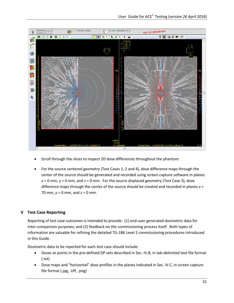
Create a 1 x 2 display grid using the grid definition tool in the toolbar.
Load axial and sagittal (or coronal) reconstructed views into the grid panels by dragging them
from the ‘Reconstructed images’ tab on the Thumbnail palette. Turn off reconstructed points
display to unclutter the dose difference display panels.
User Guide for ACE Testing (version 26 April 2016)
31
Scroll through the slices to inspect 2D dose differences throughout the phantom.
For the source centered geometry (Test Cases 1, 2 and 4), dose difference maps through the
center of the source should be generated and recorded using screen capture software in planes
x = 0 mm, y = 0 mm, and z = 0 mm. For the source displaced geometry (Test Case 3), dose
difference maps through the center of the source should be created and recorded in planes x =
70 mm, y = 0 mm, and z = 0 mm.
V Test Case Reporting
Reporting of test case outcomes is intended to provide: (1) end-user generated dosimetric data for
inter-comparison purposes; and (2) feedback on the commissioning process itself. Both types of
information are valuable for refining the detailed TG-186 Level 2 commissioning procedures introduced
in this Guide.
Dosimetric data to be reported for each test case should include:
Doses at points in the pre-defined DP sets described in Sec. IV.B, in tab-delimited text file format
(.txt)
Dose maps and “horizontal” dose profiles in the planes indicated in Sec. IV.C, in screen capture
file format (.jpg, .tiff, .png)
User Guide for ACE Testing (version 26 April 2016)
32
Dose difference maps in the planes indicated in Sec. IV.D, in screen capture file format (.jpg, .tiff,
.png)
Any other dose data highlighting an issue that you believe requires attention, in tab-delimited
text file or screen capture file format, along with a concise description of the issue
Any other dose data obtained using third-party software that you believe would improve the
commissioning process, in tab-delimited text file or screen capture file format, along with a
concise description of the improvement
Written feedback on the commissioning process itself should include:
A description of any procedural issues encountered trying to execute a Test Case import,
calculation set up, dose calculation, or dose display procedure, etc.
A description of any difficulties encountered in trying to follow the instructions in this User
Guide
Suggestions for improving the commissioning process and/or the User Guide.
User Guide for ACE Testing (version 26 April 2016)
33
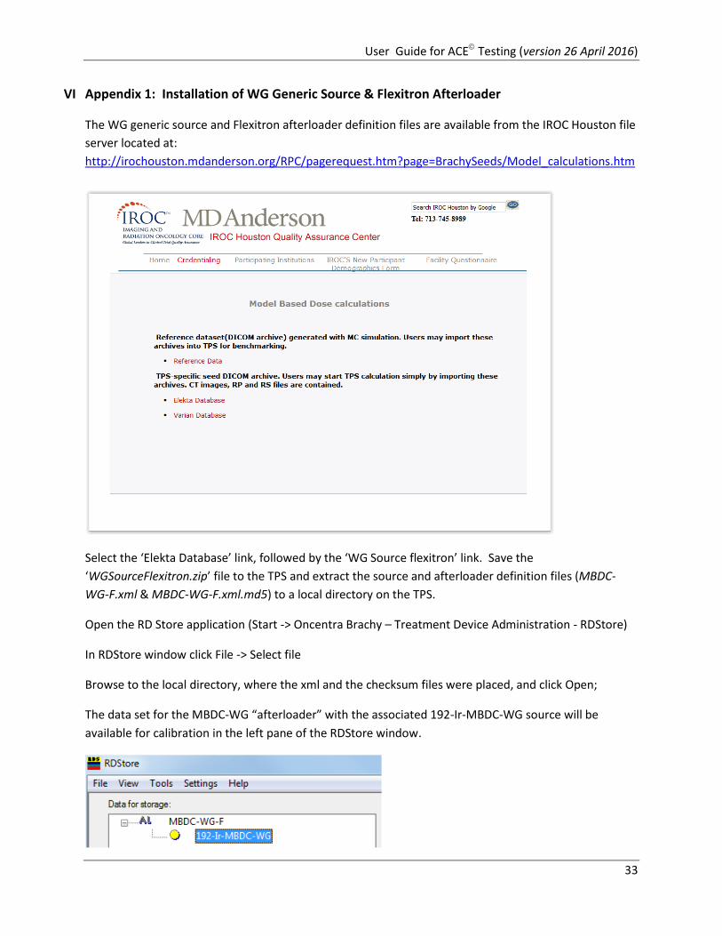
VI Appendix 1: Installation of WG Generic Source & Flexitron Afterloader
The WG generic source and Flexitron afterloader definition files are available from the IROC Houston file
server located at:
http://irochouston.mdanderson.org/RPC/pagerequest.htm?page=BrachySeeds/Model_calculations.htm
Select the ‘Elekta Database’ link, followed by the ‘WG Source flexitron’ link. Save the
‘WGSourceFlexitron.zip’ file to the TPS and extract the source and afterloader definition files (MBDC-
WG-F.xml & MBDC-WG-F.xml.md5) to a local directory on the TPS.
Open the RD Store application (Start -> Oncentra Brachy – Treatment Device Administration - RDStore)
In RDStore window click File -> Select file
Browse to the local directory, where the xml and the checksum files were placed, and click Open;
The data set for the MBDC-WG “afterloader” with the associated 192-Ir-MBDC-WG source will be
available for calibration in the left pane of the RDStore window.

User Guide for ACE Testing (version 26 April 2016)
34
Leave the afterloader name as “MBDC-WG-F”. Right click on the source name and select ‘Modify Source’
and enter the source calibration data as: Calibration Date: 01 Apr 2016, Calibration time: 10:00:00 and
Air Kerma Strength 36260.00 (cGy cm2/h) ( ~ 10Ci Apparent Activity). Click OK.
Drag and drop the “MBDC-WG-F” afterloader from the left pane to the right pane of RDStore. The
RDStore username and password will be required to confirm this transfer.
The Flexitron afterloader and WG generic source will be available in the OCB system.
Close the RDStore application.
User Guide for ACE Testing (version 26 April 2016)
35
VII Appendix 2: MCNP6 Point Dose Values
User Guide for ACE Testing (version 26 April 2016)
36
User Guide for ACE Testing (version 26 April 2016)
37
VIII References
[1] L. Beaulieu, Å. Carlsson Tedgren, J.-F. Carrier, et al, Report of the Task Group 186 on model-based
dose calculation techniques in brachytherapy beyond the TG-43 formalism: Current status and
recommendations for clinical implementation, Med. Phys. 39, 6208-6236 (2012).
[2] http://www.aapm.org/org/structure/default.asp?committee_code=WGDCAB
[3] F. Ballester, Å. Carlsson Tedgren, Domingo Granero, et al, A generic high-dose-rate 192Ir brachytherapy
source for evaluation of model-based dose calculations beyond the TG-43 formalism, Med. Phys. 42,
3048-3062 (2015).
[4] A. Ahneshö, Collapsed cone convolution of radiant energy for photon dose calculation in
heterogeneous media, Med. Phys. 16, 577-592 (1989).
[5] Å. Carlsson and A. Ahneshö, The collapsed cone superposition algorithm applied to scatter dose
calculations in brachytherapy, Med. Phys. 27, 2320-2332 (2000).
[6] L. Beaulieu, Y. Ma, R. van Veelen, ACE – Advanced Collapsed cone Engine, Elekta White Paper (2014).
[7] Oncentra Brachytherapy planning system v4.5 online help: Planning with collapsed cone dose
calculation algorithm [BP] (2014).
[8] S. B. Jiang, G. C. Sharp, T. Neicu, R. I. Berbeco, S. Flampouri, and T. Bortfeld, On dose distribution
comparison, Phys. Med. Biol. 51, 759-776 (2006).
[9] V. Peppa, E. Pantelis, E. Pappas, V. Lahanas, C. Loukas, P. Papagiannis, A user oriented procedure for
the commissioning and quality assurance testing of treatment planning system dosimetry in High Dose
Rate brachytherapy, Brachytherapy in press (2016).
[10] C. Pinter, A. Lasso, A. Wang, D. Jaffray, G. Fichtinger, SlicerRT: Radiation therapy research toolkit for
3D Slicer, Med. Phys. 39, 6332-6337 (2012).