User-Centric Modelling For Data Warehouses

Resmi Nair

Thesis

Submitted by Resmi Nair

for fulfillment of the Requirements for the Degree of

Doctor of Philosophy

Faculty of Information Technology, Monash University

June 2007

AMENDMENTS

ERRATA

p 25, line 1 ”its” for it’s

p 201, line 3 ”its” for it’s

p 57,line 7, ”latter” for ”later”

p 174, line 8, ”latter” for ”later”

p194, line 4, ”latter” for ”later”

ADDENDUM

p27, At the end of para 2: A UML based design that spans all the three phases

of the design could be found in [NJI06]. Meta models based on UML and trans-

formations using Object Constraint Language (OCL) are used here for the design.

The application of OCL can again found in [SJS06] for multidimensional model-

ing.

p27, Section 2.2, line 11: Read ”Different from above approaches.”

p93, Section 3.2, line4: Add ”and [VRTR05]” and read ”analysis processes such

as [RB03], [FJ03], [M.D04] and [VRTR05]” ...

p 137, Section 3.7, line 3: delete ”suggested”, add ”introduced” and read ”reduc-

tion algorithm were introduced in the context of.”

i

p 222, Section 6.2: Add new para: A reduction/optimization algorithm has been

proposed to optimize the proposed schema. Evaluation of the effectiveness and

precision of the algorithm is an area that requires further study.

Add new references in the reference section:

[NJI06]: N.Prat, J.Akoka and I.Comy-Wattiau, A UML based data warehouse

design method, Decision Support Systems, Vol 42 Issue 3, 2006.

[SJS06]: S. Lujan-Mora, J.Trujillo, Il-Yeol Song, A UML profile for multidimen-

sional modeling in data warehouses, Data and Knowledge Engineering, Vol 59 No

3, pp.725-769, 2006.

[VRTR05]: V.Nassis, R.Rajugan , T.S.Dillion, W.Rahayu, A Requirement En-

gineering Approach for Designing XML-View Driven, XML Document Ware-

houses, In International Computer Software and Applications Conference, pp.

388-395, 2005.

ii

DEDICATION

This thesis is dedicated to our loving father

iii

Declaration

I here by declare that this thesis contains no material which has been accepted for

the award of any other degree or diploma at any university or equivalent institution

and that to the best of my knowledge and belief, this thesis contains no material

previously published or written by another person, except where due reference has

been made.

Resmi Nair

June 2007

iv

Publications

Closing the Gap: Requirement of a Conceptual Model: Resmi Pillai, Bala

Srinivasan, Issues in Information Systems, Vol:3, pp 504-509, 2002

A Conceptual Query- Driven Design Framework for Data warehouse: Resmi

Nair, Campbell Wilson and Bala Srinivasan, Transactions on Engineering, Com-

puting and Technology, Vol:19, pp 141-146, 2007

v

Acknowledgement

A research project of this magnitude would not have been possible without the

support of many individuals.

My first and foremost gratitude goes to my main supervisor Prof. Bala Srini-

vasan for his support and guidance. At times when I was at crossroads, wondering

which way to go, Srini guided me on the right path. His valuable suggestions and

feedback immensely helped me to complete the thesis. I am also grateful to my

other supervisor Dr. Campbell Wilson for his contributions during research dis-

cussions. Those meetings helped me to formalise ideas and writing up of the

thesis.

I thank my fellow researchers Guy, Samar and Viranga for their help during

these years. I also thank Oshadi, my room-mate; she was there for me during

some difficult periods in my research.

A “big thank you” to Gerry for correcting my initial drafts and assisting me

with mathematical notations. I would like to thank CSSE administration and tech-

vi

nical staff for their support during my candidature.

I must acknowledge the love and support from my friends, who helped me to

pass through the research pressure. It is hard to mention all of them but Gayika is

special. She is there always, wholeheartedly, offering her helping hands.

I thank my loving parents, whose aspirations inspired me to set higher goals.

They have been supporting whatever I decided to do. For them, this is a dream

come true. Special thanks to my sister, I owe her a lot. My niece, nephew, grand

mother, brother-in-law and other family members loved me and supported me in

all my endeavors. I take this opportunity to remember my brother, who left us

nine years ago. He would have been proud of his sister achieving this great feat.

I need to thank my little girl, Anita, for her unconditional love and understand-

ing. She would have wished her mum to be with her during moments of glory at

school. She is very proud of her mum.

Finally, I thank my wonderful husband for his support. He shared my sorrows,

and taught me to be positive in life. He is my best friend and critic.

vii

Abstract

Data warehouses are the primary source for a consolidated view of enterprise

wide data which aids organisations in their decision making process. The data

in a data warehouse is populated from the instances of operational systems and

is made available to the users for their analytical needs. A number of back-end

and front- end tools are used for data acquisition and analysis. Hence the data

warehouse schema design is primarily driven by the functionalities of those tools

as well as a model for representation of data in data warehouses. So the schema

design is characterised more by the implementation models rather than by concep-

tual requirements. In principle, a data warehouse can be viewed as an aggregated

database and hence its schema design does need to take into account the users’

needs and requirements. Generally the users requirements are expressed in terms

of queries. Hence there is a need to formally define classes of queries and for-

mulate a systematic and iterative approach to synthesising the schema from the

user specifications. The design should be general and independent so that it can

viii

be translated to logical and physical phases.

This thesis proposes a model for capturing user queries and a method of syn-

thesising data warehouse schemas. In order to provide a query model, a taxonomy

of data warehouse queries is studied and has been classified so that this synthesis

is correct and complete. The proposed design allows query specification in natural

language form. To translate these queries into a schema, a formal representation

is required. Hence a query representation is proposed which aids the schema gen-

eration process. Formal discussion on the design is adequately supported by real

life examples and a case study is provided for this purpose.

Recognising the advantage of an information model at the conceptual phase,

we have introduced such a model in our design. This serves as a common platform

for various data warehouse schemas with specific properties and the designer is

able to derive schema based on demand.

The generality of our model is described in terms of subsuming other models.

Hence mapping techniques are detailed and particular implementation issues are

discussed. The proposed design follows the guidelines of traditional conceptual

design where by the conceptual phase is independent of the logical and physical

levels. The notion of independence is further extended towards the conceptual

level, providing a method for schema refinement with respect to relevant opti-

mization criteria for data warehouses. The design is comprehensive yet practical,

in the sense that it provides query specific schema for implementation.

ix

Contents

1 Introduction 1

1.1 Data Warehousing: A Business Intelligent

System . . . . . . . . . . . . . . . . . . . . . . . . . . . . . . . . 3

1.1.1 Architecture of Data Warehousing . . . . . . . . . . . . . 5

1.2 Data Warehousing Issues . . . . . . . . . . . . . . . . . . . . . . 12

1.2.1 Design Issues . . . . . . . . . . . . . . . . . . . . . . . . 15

1.3 Motivation . . . . . . . . . . . . . . . . . . . . . . . . . . . . . . 16

1.4 Objectives and Contributions . . . . . . . . . . . . . . . . . . . . 20

1.5 Thesis Structure . . . . . . . . . . . . . . . . . . . . . . . . . . . 21

1.6 Summary . . . . . . . . . . . . . . . . . . . . . . . . . . . . . . 23

2 Data Warehouse Design 24

2.1 Introduction . . . . . . . . . . . . . . . . . . . . . . . . . . . . . 24

2.2 Data Warehouse Design: An Overview . . . . . . . . . . . . . . . 26

2.2.1 Top-down and Bottom-up Designs . . . . . . . . . . . . . 28

x

2.3 Design Considerations . . . . . . . . . . . . . . . . . . . . . . . 30

2.3.1 Multidimensional Representation . . . . . . . . . . . . . 31

2.3.2 Aggregation . . . . . . . . . . . . . . . . . . . . . . . . . 32

2.3.3 Business Measures . . . . . . . . . . . . . . . . . . . . . 36

2.3.4 Hierarchies . . . . . . . . . . . . . . . . . . . . . . . . . 38

2.3.5 Aggregation Along a Hierarchy . . . . . . . . . . . . . . 44

2.3.6 Source Data . . . . . . . . . . . . . . . . . . . . . . . . . 46

2.4 Data Warehouse and Queries . . . . . . . . . . . . . . . . . . . . 47

2.4.1 User-Centered Schema Design . . . . . . . . . . . . . . . 48

2.4.2 Query Based Approaches . . . . . . . . . . . . . . . . . . 49

2.4.3 Query Types . . . . . . . . . . . . . . . . . . . . . . . . 52

2.5 Top-down Designs . . . . . . . . . . . . . . . . . . . . . . . . . 55

2.5.1 Cube Models . . . . . . . . . . . . . . . . . . . . . . . . 56

2.5.2 Extended ER Models . . . . . . . . . . . . . . . . . . . . 60

2.5.3 Other Approaches . . . . . . . . . . . . . . . . . . . . . 64

2.6 Bottom-Up Designs . . . . . . . . . . . . . . . . . . . . . . . . . 69

2.6.1 ER to Dimensional Fact Model . . . . . . . . . . . . . . 70

2.6.2 ER to Multidimensional Model . . . . . . . . . . . . . . 72

2.6.3 ER to Star . . . . . . . . . . . . . . . . . . . . . . . . . . 74

2.6.4 ER to Multidimensional ER . . . . . . . . . . . . . . . . 77

2.6.5 A Hybrid Approach . . . . . . . . . . . . . . . . . . . . . 79

xi

2.7 Towards a Query Oriented Schema Design . . . . . . . . . . . . . 81

2.8 Summary . . . . . . . . . . . . . . . . . . . . . . . . . . . . . . 89

3 User-Centric Schema Design Framework 90

3.1 Introduction . . . . . . . . . . . . . . . . . . . . . . . . . . . . . 90

3.2 Formalisation of Requirements . . . . . . . . . . . . . . . . . . . 93

3.2.1 Definition: Measure Type . . . . . . . . . . . . . . . . . 95

3.2.2 Derived Measure Type . . . . . . . . . . . . . . . . . . . 96

3.2.3 Similarity between Measure Types . . . . . . . . . . . . . 100

3.2.4 Classification . . . . . . . . . . . . . . . . . . . . . . . . 101

3.3 The Knowledge Base Graph . . . . . . . . . . . . . . . . . . . . 111

3.4 Query Representation . . . . . . . . . . . . . . . . . . . . . . . . 119

3.5 Query Taxonomy . . . . . . . . . . . . . . . . . . . . . . . . . . 122

3.5.1 Single Measure Type-Single Classification (Type SS) . . 125

3.5.2 Single Measure Type-Multiple Classification (TypeSM ) . 128

3.5.3 Multiple Measure Type (TypeMM ) . . . . . . . . . . . . 130

3.5.4 Query with only one Measure Type (Type M) . . . . . . . 131

3.5.5 Query with Specialized Class (Type S) . . . . . . . . . . 132

3.5.6 Query with Exception (Type E) . . . . . . . . . . . . . . 132

3.6 The User-Centered Schema Design Framework . . . . . . . . . . 135

3.7 Summary . . . . . . . . . . . . . . . . . . . . . . . . . . . . . . 139

xii

4 Translation of Queries for Schema Synthesis 141

4.1 Introduction . . . . . . . . . . . . . . . . . . . . . . . . . . . . . 141

4.2 Intermediate Schema Using Queries . . . . . . . . . . . . . . . . 143

4.3 Mapping Query Trees . . . . . . . . . . . . . . . . . . . . . . . . 148

4.3.1 Validation and Classification of Query Trees . . . . . . . 152

4.3.2 Similarity Function . . . . . . . . . . . . . . . . . . . . . 154

4.4 TypeSS Queries and the Mapping . . . . . . . . . . . . . . . . . 158

4.4.1 MappingTypeSS1 Queries . . . . . . . . . . . . . . . . 158

4.4.2 MappingTypeSS2 Queries . . . . . . . . . . . . . . . . 164

4.4.3 MappingTypeSS3 Queries . . . . . . . . . . . . . . . . 167

4.5 TypeSM Queries and the Mapping . . . . . . . . . . . . . . . . 168

4.5.1 MappingTypeSM1 Queries . . . . . . . . . . . . . . . . 168

4.5.2 MappingTypeSM2 Queries . . . . . . . . . . . . . . . . 170

4.5.3 MappingTypeSM3 queries . . . . . . . . . . . . . . . . 171

4.6 Mapping Other Query Types . . . . . . . . . . . . . . . . . . . . 172

4.6.1 MappingTypeMM queries . . . . . . . . . . . . . . . . 172

4.6.2 Mapping Exception Queries . . . . . . . . . . . . . . . . 173

4.6.3 Reconsidering Rejected Queries . . . . . . . . . . . . . . 175

4.7 The Intermediate Schema . . . . . . . . . . . . . . . . . . . . . . 176

4.8 Summary . . . . . . . . . . . . . . . . . . . . . . . . . . . . . . 181

xiii

5 Synthesis of Intermediate Schema 182

5.1 Introduction . . . . . . . . . . . . . . . . . . . . . . . . . . . . . 182

5.2 Mapping of Intermediate Schema to Existing DW Models . . . . 184

5.2.1 Cube Design Using Intermediate schema . . . . . . . . . 184

5.2.2 Mapping to Star-schema . . . . . . . . . . . . . . . . . . 198

5.2.3 Discussion . . . . . . . . . . . . . . . . . . . . . . . . . 204

5.3 Conceptual Reduction . . . . . . . . . . . . . . . . . . . . . . . . 205

5.3.1 The Reduction Algorithm . . . . . . . . . . . . . . . . . 208

5.4 Summary . . . . . . . . . . . . . . . . . . . . . . . . . . . . . . 215

6 Conclusion and Future Work 217

6.1 Conclusion . . . . . . . . . . . . . . . . . . . . . . . . . . . . . 217

6.2 Future Research . . . . . . . . . . . . . . . . . . . . . . . . . . . 220

References 223

Appendix A Proof: Classification Lattice 243

Appendix B TypeSS2 Mapping 252

Appendix C TypeSS3 Mapping 255

Appendix D TypeSM1 Mapping 257

Appendix E TypeSM2 Mapping 259

xiv

Appendix F TypeSM3 Mapping 262

Appendix G Intermediate Schema : An Example 264

xv

List of Figures

1.1 Data warehousing architecture. . . . . . . . . . . . . . . . . . . 6

2.1 A data cube: multidimensional view. . . . . . . . . . . . . . . . 33

2.2 Requirements: different point of views. . . . . . . . . . . . . . . 36

2.3 Multiple hierarchies: an example. . . . . . . . . . . . . . . . . . 42

3.1 Classification schema: an example . . . . . . . . . . . . . . . . . 104

3.2 A grouping function . . . . . . . . . . . . . . . . . . . . . . . . 105

3.3 An example classification lattice . . . . . . . . . . . . . . . . . . 108

3.4 Representation of descriptive attributes . . . . . . . . . . . . . . 110

3.5 The KB Graph: an example . . . . . . . . . . . . . . . . . . . . 116

3.6 A KB graph: from Case Study . . . . . . . . . . . . . . . . . . . 117

3.7 Edges in KB graph . . . . . . . . . . . . . . . . . . . . . . . . . 118

3.8 A Query tree from Case Study. . . . . . . . . . . . . . . . . . . . 122

3.9 A query taxonomy. . . . . . . . . . . . . . . . . . . . . . . . . . 124

3.10 The user-centered schema design framework . . . . . . . . . . . 136

xvi

4.1 TypeSS1 query tree . . . . . . . . . . . . . . . . . . . . . . . . 163

4.2 TypeSS2 query tree . . . . . . . . . . . . . . . . . . . . . . . . 167

4.3 TypeSS3 query tree . . . . . . . . . . . . . . . . . . . . . . . . 168

4.4 TypeSM1 query tree . . . . . . . . . . . . . . . . . . . . . . . . 169

4.5 TypeSM2 query tree . . . . . . . . . . . . . . . . . . . . . . . . 171

4.6 TypeSM3 query tree . . . . . . . . . . . . . . . . . . . . . . . . 172

4.7 Intermediate schema: an example. . . . . . . . . . . . . . . . . . 177

5.1 Star constellation: an example. . . . . . . . . . . . . . . . . . . . 202

5.2 Star galaxy: an example. . . . . . . . . . . . . . . . . . . . . . . 203

5.3 Minimal DW schema: an example. . . . . . . . . . . . . . . . . 212

G.1 An intermediate schema from case study . . . . . . . . . . . . . 266

xvii

List of Algorithms

4.1 Intermediate Schema Algorithm . . . . . . . . . . . . . . . . . . 148

4.2 MappingTypeSS1 Queries . . . . . . . . . . . . . . . . . . . . . 162

5.1 Dimension Selection Algorithm . . . . . . . . . . . . . . . . . . 196

5.2 Reduction Algorithm . . . . . . . . . . . . . . . . . . . . . . . . 211

1

Chapter 1

Introduction

Businesses around the world are undergoing a transformation caused mainly by

globalisation and economic changes. They are forced to change their conventional

business processes to become more agile and efficient. A new breed of managers

calledmultidimensional managers([RNR99]) have emerged to tackle the current

challenges. These multidimensional managers operate in a business world that is

complex and possess a multidimensional view of their business. They are chang-

ing the traditional way of hierarchical management to a horizontal network where

the interests of managers span the whole business itself.

Most organisations will have multiple business applications that improve the

efficiency of managerial and operational processes of various business units. These

business applications create enormous amount of data which in most cases are

purged out after a certain period. The strategic value of the data is being recog-

1

nised and efforts are focused towards extracting the value to gain competitive

advantage. A new generation of systems calledbusiness intelligent (BI) systems

or analytical systemshave come into existence as a result of this. Organisations

benefit from improved customer service, effective marketing programs, accurate

demand forecasting and an overall cost savings due to operational efficiencies be-

stowed from BI systems.

BI systems are primarily focussed on processing the existing enterprise data to

provide high-quality information to people throughout the organisation. In other

words, BI systems gather, manage and analyse data to provide insight into trends

and opportunities. It is assumed that any knowledge worker is able to access

information from these systems.

In this thesis we analyse one such BI system calledData Warehousing; which

is also used for decision making processes. This is an environment rather than a

product [K.J98], in which various components are involved and in the following

sections we will describe data warehousing and its functionalities in detail.

This chapter is organised as follows. In Section 1.1, the data warehousing

environment is introduced. In subsequent subsections, different stages associated

with this system are explained. Various issues associated with the system devel-

opment are discussed in Section 1.2. From these addressed issues, one particular

aspect; data warehouse design, which is the primary focus of the thesis, is consid-

ered in detail. Thesis motivations and the contributions are explained in Section

2

1.3 and Section 1.4 respectively. The thesis organisation is explained in Section

1.5 and the chapter is concluded in Section 1.6

1.1 Data Warehousing: A Business Intelligent

System

“Data warehousing is defined as a process for assembling and managing data from

various sources for the purpose of gaining a single, detailed view of a part or all

of a business” [S.R98]. A centralised repository calleddata warehouseis used

to provide the integrated view of data. It can also be described as a dedicated

database which provides relevant information to decision makers.

The demand for this technology is stronger ever since the concept emerged

in the early nineties. According to the Gartner group survey in 2004, ([Rel06]),

data warehousing came into the top ten priorities among CEOs. Organisations are

investing in data warehousing as they consider data as their asset.

Case studies from different business areas illustrate success stories of data

warehousing. An American retail company [LC04], implemented a data ware-

house in 1995 and captured many customer interactions. This enabled the com-

pany to gain customer intimacy and thereby segmenting their customer portfolio.

3

In addition, the data warehouse allowed the company to improve their cus-

tomer relationship management as well as marketing opportunities.

Mercy Care Plan([Cor04]) is the second largest health care plan in Arizona.

By implementing a data warehouse they improved their customer analysis, con-

trolled their expenses and thus made an over all improvement in the business. In

the case ofFirst American Corporation[BHBD00], strategies were shifted from

traditional banking to a more customer oriented approach with the help of a data

warehouse and this implementation helped them to emerge as a leader in financial

industry.

In the past, it has been very difficult to get an integrated view of activities that

occurred in an enterprise. Previously, the information has been gained from vari-

ous source systems or production systems calledOn-line Transaction Processing

(OLTP) systems, only after someone requested for information. This is a time

consuming process and termed as alazy approach [J.W95]. Data warehousing

provided a solution to this problem in which data from different sources is inte-

grated into a single, centralized repository ready for querying. Compared to the

lazy approach mentioned earlier this one is aneagerapproach because data is

already there to answer queries.

Different types of tools are necessary in order to integrate data from various

sources as well as for the presentation of data in a warehousing environment.

These tools can be classified asback-endandfront-endtools. Back-end tools are

4

used to integrate data from heterogenous sources whereas front-end tools help to

access data from data warehouses. A more detailed discussion of tools associated

with data warehousing can be found in the following section. It also discusses

different stages associated with data warehousing in detail.

1.1.1 Architecture of Data Warehousing

The figure 1.1, divides data warehousing into three stages which can be described

as follows.

• Data acquisitionstage: During this stage data is extracted from sources,

transformed and loaded into a database using various tools.

• Data storage: At this stage, data is stored in a database.

• Data analysis: This is the final stage in which data is accessed through

analysis tools.

Each stage is explained in detail in the following sections.

Data Acquisition

A data warehouse contains data from multiple operational systems and external

sources. Since this data is used for decision making, it is important that the data

should be correct and consistent. Inconsistent field lengths and inconsistent de-

5

External Sources

Operational databases

Extraction Transformation

Load

Data warehous e

OLAP

Data Mining Serve

Data Aqusition Data Storage Data Analysis

Figure 1.1: Data warehousing architecture.

scriptions are some of the common data errors. A common example of an incon-

sistent description is the gender specification in various systems. It can bemale

and femalein certain systems orM andF in some other systems. But in a data

warehouse every piece of data can have only one meaning and specification. A

variety of tools are utilised for data cleaning, transforming and loading in order to

provide correct data in the data warehouse . These tools are collectively known as

Extract, TransformandLoad (ETL) tools.

After extraction, cleaned and transformed data is loaded into a data warehouse.

Before data loading, an additional requirement such assummarisationis required.

Summarisation refers to processing of raw input data or detail data for more com-

pact storage in a form useful for analysis in a particular application. This involves

selection, filtration, reorganization and manipulation etc, of atomic data to pro-

duce predetermined totals [S.R98].

6

A data warehouse stores historical data hence the volume of data is high. Be-

cause of this summarization is necessary. This also improves the responsiveness

of a data warehouse by improving the query response time. Two main factors

involved with summarisation are; the selection of data to summarise and the unit

of time for summarization. These factors are decided by a designer based on the

nature of the queries that need to be answered.

As we mentioned earlier, data from a data warehouse comes from operational

systems. This means the changes happening at this level need to be propagated

to the data warehouse after the data warehouse is populated. Sending updates

to a data warehouse is calledrefreshingand the tools used for this purpose are

called refresh tools. The refreshing of a data warehouse is an important process

which determines the effective usability of data collected and aggregated from the

sources [BFMB99]. The refresh frequency is normally set by an administrator

based on user needs and source systems.

Data Storage

As mentioned in Section 1.1, a data warehouse is a dedicated database used for

decision making processes. The characteristics of a data warehouse are considered

here in detail. A well cited reference for data warehouses comes from [W.H92].

Inmon defined data warehouse (DW) as a subject oriented, integrated, time variant

and non-volatile collection of data. The definition is further detailed as:

7

• Subject orientation: In a data warehouse, data is organised in subject areas

like finance, sales etc across the enterprise whereas operational systems are

typically designed in the context of an enterprise’s applications such as pay

roll, order entry, etc.

• Integration: Data from various heterogenous sources are integrated in a data

warehouse. The sources of a data warehouse normally are the underlying

operational systems, external data sources etc. Data in a data warehouse is

homogenized and cleaned which allow querying from a common repository.

Data warehouse data varies ingranularity. That is, data in a data warehouse

ranges from the most detailed level to a highly summarized level. Raw data

from the operational systems is considered to be the most detailed level.

• Time-invariant: Generally data in a data warehouse are stored as snapshots

and not on current status. This historical data can then be analysed in order

to ascertain business trends.

• Non-volatility: Data in data warehouse is read only; users are not allowed

to change the data. Modifications in data warehouse data takes place only

when the modifications of the source data are loaded into the data ware-

house.

Even though data warehouse is derived from operational data, it is different

from the operational databases. The design of a data warehouse is more chal-

8

lenging than that of operational databases because of the nature of the system and

the volume of data involved. Also the functionalities of these two databases are

different. Maximizing transaction through-put and minimizing conflicts are the

main criteria for operational databases whereas data warehouses aim to support a

smaller number of users in their decision making. Since data warehouses are used

for analysis purposes they are also known asanalytical databases.

The following Table 1.1 shows the main differences between a data warehouse

and an operational database.

Operational database Data warehouseTransaction driven Analysis drivenSupport day-to-day operationSupport decision makingConstant updates Updates are rareDetailed data Summarized dataCurrent data Historical dataDeals with few records Deals with millions of

recordsLarge number of users Smaller number of users

Table 1.1: Operational database vs Data warehouse

Data Analysis

Data analysis refers to access data from data warehouses for decision making

processes. Two major application areas of a data warehouse are Online Analytical

Processing( OLAP) and Data Mining.

9

OLAP : In 1993 E.F. Codd introduced the term OLAP for intuitive, interactive

and multidimensional analysis of data [ESC93]. That is, OLAP is characterized by

the multidimensional representation (presenting data as a multidimensional space)

and analysis of consolidated enterprise data which supports end users analytical

and navigational needs. As pointed out in [BCGM98], during the last decade there

was a rapid growth in this area. OLAP has become very popular primarily because

of the features it offers to the users. The features are: visualization, navigation and

sophisticated analysis [N.G03]. Visualization allows the user to interact with the

system in a user friendly manner. Navigation refers to operations by which users

are able to view data with different granularity. Sophisticated analysis allows

users to perform different types of analysis such as statistical profiling, moving

averages, exception conditions etc.

OLAP tools are mainly classified in terms of the underlying data warehouse

implementation. They are calledRelational OLAPandMulti dimensional OLAP.

• ROLAP: Data warehouses might be implemented on standard or extended

relational databases calledRelational OLAPor ROLAP ([SU97]). One ma-

jor issue with this implementation is expressing the operations. OLAP op-

erations can not map efficiently into relational operations. In other words,

using standard SQL it is difficult to express an OLAP query. Many com-

mercial products extended SQL to incorporate OLAP operations. However

10

this drastically reduces system performance [LJ00]. Even with this limita-

tion, the relational implementation is considered as good for very large data

warehouses.

MicroStrategy’s DSS server ([Mic98]) and Informix’s Meta Cube ([IBM98])

are examples of commercially available ROLAP.

• MOLAP: If data warehouses use a specific data management system in

terms of array structure it is calledMulti dimensional OLAPor MOLAP.

Since arrays are used for data storage, empty cells are possible resulting in

sparse data. Storing sparse data is inefficient and additional compression

techniques are necessary to overcome this limitation [BCGM98]. Nonethe-

less MOLAP efficiently supports OLAP operations and is suitable for data

warehouses where the amount of data is considerably low.

Hyperion Essbase from Hyperion ([Hyp01]) is an example of a commer-

cially available MOLAP product.

Data Mining : The OLAP application, that we have discussed previously,

deals with users on-line analysis requirements. In this case users’ involvement

is mandatory. When dealing with large amounts of data, this manual analysis

becomes slow and expensive. Businesses consider data as their asset and it is

used to increase their efficiency and success. Hence computational techniques

are necessary to get valuable information from the data. Data mining is one such

11

technique which is used to identify patterns from mass volume of data. Data

mining is a generic term used for the application of specific algorithms for ex-

tracting patterns from data. This is considered as a step in Knowledge Discovery

in Databases (KDD). KDD is defined as the nontrivial process of identifying valid,

novel, potentially useful, ultimately understandable patterns in data [UGSP96a].

Commonly used data mining algorithms for this purpose are: classification, re-

gression and clustering [UGSP96b]. Future trends and interesting patterns of a

business can be extracted from a data warehouse using these mining techniques.

In this section we have studied data warehousing, in particular the stages as-

sociated with the system. Based on this we will discuss various research areas

associated with data warehouse system development in the next section.

1.2 Data Warehousing Issues

In the previous section we have seen different stages of data warehousing in terms

of data acquisition, storage and analysis. Each of these stages present various

challenges. In order to tackle this, different streams of research areas have been

evolved. They are mainly focussed on issues related to design, implementation,

operation and maintenance. The main goal of all these areas is to provide neces-

sary information to the user correctly and quickly.

12

Based on the general architecture discussed in Section 1.1.1, different research

problems are illustrated here. The main issue associated with the first stage can be

seen asdata integration and loading[J.W95], [J.S99]. Data integration is a dif-

ficult process because of the inconsistencies in source databases. Since different

types of data sources are involved, schema integration is the major issue. Tools

development related to data integration and translation is also challenging.

Query processing and optimization has been of keen interest to researchers

[SU97]. Since a data warehouse is primarily used as a source for querying, queries

are important in this environment. Compared to the update and deletion queries in

traditional databases, data warehouse queries are complex. Queries are complex

in the sense that they consist of common functions such assum, count, minimum,

maximum etcas well as complex statistical functions likemedian or moving av-

erage etc. Moreover, as the size of the database is in gigabyte to terabyte range,

the join operation becomes a more costly procedure than the update and deletion

queries. The well known query language, SQL does not allow the concise expres-

sion of queries involving aggregation and group-by [CR96]. In order to express

such queries, extension of SQL is required. Because of these reasons query pro-

cessing and optimization need more sophisticated techniques and approaches like

[AVD95], [JWWL00], [SS96] and [DA01] contributed towards this area.

With respect to maintenance and operation of a data warehouse,view mainte-

nanceis one area to consider [DASY97], [RAX00] [DM00] and [RC03]. As we

13

mentioned earlier, a data warehouse stores integrated information from multiple

data sources. The integrated information is normally in a pre-computed form in

order to improve the query response time. This pre-computation is calledmate-

rialising viewsover source data. Hence in an abstract level, data in a data ware-

house can be seen as a set of materialised views. The challenges associated with

this technique are:

• selection of views to materialise: A materialised view is normally treated

as a pre-computed query or a partial query. That means view selection de-

pends on those queries which need to be answered. While the view selec-

tion, generally minimum query evaluation cost will be the main criterion

and storage space could be another consideration. Pre-computing all the

expected queries is ideal but space constraint has to be considered. The

challenge here is to select views with minimum query evaluation cost for

given system constraints.

• efficient use of the materialised views: One view will be able to answer

different queries. In that respect techniques are necessary for the efficient

use of the views.

• efficient update of materialised views according to the changes in source

data: The main issue associated with the view technology is that views

need to be updated according to the source.

14

If the frequency of updates are high the maintenance cost will increase

which is not desirable.

Various approaches studied the above mentioned issues and a few examples are

[CMJ01], [RHD02], [HM99], [SKSK95] and [DASY97].

Since data warehouse is considered as the main component of the system, its

design is very important. This is considered in detail in the next section.

1.2.1 Design Issues

The design of data warehouse itself is challenging in the second stage. This in-

cludes all the phases of design, from conceptual to physical implementation. Even

though data warehouse design is similar to operational databases, the techniques

used in the design of these databases are not suitable for a data warehouse. This is

mainly due to the differences in functionalities that we have summarised earlier in

Section 1.1.1. Different from OLTP databases, a data warehouse needs to support

OLAP applications which include navigation and complex analysis.

In the past few years research in this area has flourished. Approaches such as

[WWAL02] and [SMKK98] identified issues associated with conceptual model-

ing in terms of representation and summarisation. However we could find more

focussed designs in [TC99], [AKS01] and [CMGD98] where the interest is the

conceptualisation itself. Another set of works; for example [D.l00], [MDS98b],

15

known as methodologies, studied the transformation of an ER model to a data

warehouse model. These designs assume the existence of an ER model and guide-

lines are provided to identify the data warehouse constructs from this.

Issues related to implementation such as efficient data structures and new in-

dexing techniques are the focus of physical design. Here we avoid a detailed dis-

cussion on physical design to concentrate on the conceptual side. However, read-

ers could find studies specific to physical aspects in [VAJ96], [MDA01], [LJY03],

[MZ00], [HVAJ97], and [WDB97].

1.3 Motivation

We have addressed various issues associated with data warehousing in the previ-

ous section. Here we further investigate issues related to conceptual design which

form the basis of this thesis.

At the beginning research in conceptual design was focussed on operators/

algebra . Approaches such as [RGS97], [LW96] [P.V98], [AH97] and [ML97] are

example of this. In [AJS01] these models are calledformalismsdue to the lack of

semantic richness.

More semantically rich models; [CMGD98], [JMJS01], came later and these

approaches extended the existing ER or object-oriented concepts in order to cap-

ture data warehouse requirements. A common feature of all these models is the

16

multidimensional data representation (discussed in detail in Chapter 2), which is

the natural way the user perceives the problem at hand.

The current models addressed a set of analysis requirements related to naviga-

tion and data summarization. These approaches provide their own formalisations

and graphical notations which means there is no standardisation in this regard.

Also, these designs terminate with the conceptualisation of analysis require-

ments. A design process is not complete without schema derivation and evalua-

tion. As pointed out in [HLV00], the existing data models were developed without

an associated design process and thus without guidelines on how to use them or

what to do with the resulting schema.

When comparing data warehouse design with traditional database design, the

transition of a model to a schema is not seamless. In traditional database design

there are pre-defined objectives associated with each stage of a design. For exam-

ple, completeness with respect to application domain, minimality of the schema,

freedom of redundancy etc are the objectives associated with conceptual design

[HLV00]. The dependency theory ([C.J00]), further explains the need for redun-

dancies and normal forms are suggested to eliminate them. A similar systematic

approach could not be found in data warehouse design. Normal forms are studied

in the context of data warehouse data models in [WJH98]. However this approach

applied normal forms only to avoid specific issues related to data summarisa-

tion. Functional dependencies are applied in [HLV00] to derive a data warehouse

17

schema from an ER model. Taking all these aspects into account, the motivations

of this thesis are as follows.

• Even though the existing designs such as [TC99], [AKS01] and [Leh98],

addressed the issues related to visualization and navigation along the data,

a formal foundation is still missing. A model that can act as a basis for

generating schema with particular characteristics is lacking. This is noted

in [A.A02] that “it is difficult to identify a standard data model, because

there is neither a model encompassing the semantic constructs of the rest,

nor a consensus or standard for what should be represented in a schema ”.

To this extent a generalisation is necessary.

• Another set of designs called methodologies or bottom-up designs could be

found in this area. These methodologies ([MDS98a], [LR98], [D.l00]) pro-

vide design guidelines to construct a data model from an existing global ER

model of the operational systems. In these bottom-up design approaches

the modeling constructs are pre-defined and they are identified from an ER

model. The main drawback of these methodologies is that, a data warehouse

is derived based only on the operational systems. Data warehouses need ex-

ternal data like web data and market survey data. External data representa-

tion is not taken into consideration in current methodologies. Discussion on

user requirements and a method to translate those requirements to a schema

18

are also lacking here. So, to summarise, bottom-up designs are data driven

and a user oriented approach is necessary.

• Complex query support is the main function of a data warehouse. The anal-

ysis requirements presented in existing models originate from the queries

but real queries are given very little importance during the conceptuali-

sation phase. As per current philosophy ([CMGD98], [MDS98a]), a data

model captures certain analysis requirements which are only a higher level

abstraction of real user requests. The user then formulates queries based on

this model and the query support is left out as a post design problem. What

we argue here, is that user queries should be taken into consideration while

designing the schema even though not all queries are known at the early

stage. By doing so the schema becomes more user oriented and is easier to

support those types of queries that are considered during the design. This

approach also allows easy translation of the schema to logical and physical

levels.

In order to provide such a technique, data warehouse queries need to be stud-

ied from a conceptual perspective. Currently the query discussions presented are

mainly related to optimization and processing. So far, a study on queries at the

conceptual level and impact of different types of data warehouse queries in schema

19

design have not been considered. However, these are issues which require in-

vestigation.

1.4 Objectives and Contributions

This thesis addresses the previously discussed problems, by providing a modelling

framework which supports a conceptual schema design for a data warehouse. The

framework is general enough to support a wide range of business applications.

The concepts and the techniques are presented formally in this framework. This

formalisation will map user requirements into a conceptual schema.

A discussion on schema properties and the derivation of a data house schema

can be seen as an optimisation approach at the conceptual level. But the optimisa-

tion part does not deviate from conceptual end to physical end. We emphasize here

that the term optimisation refers only to conceptual restructuring and all the opti-

misation properties are discussed purely at the conceptual level. Any assumptions

or considerations of physical properties cannot be seen in this approach. Based on

the above discussion, the main contributions of this thesis are as follows.

• A modeling framework is proposed based on requirements that support

a data warehouse conceptual schema design. This proposed design uses

queries for schema synthesis, so a query efficient schema can be generated.

In addition to this the design fulfills generality and independence properties.

20

• Data warehouse queries are studied from a conceptual perspective. A tax-

onomy and a conceptual representation for queries are developed based on

this study and are used in the design for schema derivation.

• We propose a generalisation of existing data warehouse data models. While

the existing models use specific modelling techniques such as ER and Object-

oriented, we choose a graph theory approach for the formalisation. This

serves the purpose of generality of the data structure and can be fitted into

the proposed framework. Graph reduction techniques are applied to produce

the final data warehouse schema.

1.5 Thesis Structure

In order to investigate more about data warehouse design, in Chapter 2, the ex-

isting designs are reviewed. Since our focus is on requirement oriented schemas,

current models have been approached from a requirements point of view. Another

highlight of this chapter is a discussion on data warehouse queries. This study

leads to a formal query taxonomy and a conceptual representation.

Chapter 3 begins with formal definitions and formalisation of concepts that

are necessary for our design. For the formalisation, a graph theory approach is se-

lected to keep the framework as general as possible. This formalisation is termed a

knowledge base, which is treated as the basic knowledge required for the schema.

21

Other than this, a conceptual perspective on queries is presented which consists of

a taxonomy and a conceptual representation.

Chapter 4 describes a schema generation method using queries. An algorithm

is developed for this purpose which maps different types of queries in the knowl-

edge base. Mapping methods associated with each query type are described in

detail. A special type of function called similarity function is suggested to aid

the mapping process, the main functionality being to test the similarity that exists

between the nodes in the graph.

Chapter 5 is presented as two parts. The first part discusses the mapping of

intermediate schema to the existing models. This mapping shows the complete-

ness and generality of the proposed framework. Algorithms are developed to map

the graph based schema to the cube and star models. In the mapping, various

implementation issues are also considered.

The second part of this chapter discusses schema refinement. This is proposed

as a conceptual reduction where a graph reduction method is suggested to derive a

data warehouse schema. The proposed reduction algorithm finds the shortest path

for a query which is will be the schema property.

A retail case study is adopted to describe the design and is used as a running

example of this thesis.

Chapter 6 concludes the thesis and future works are detailed.

22

1.6 Summary

Data Warehousing has been introduced as a business intelligent system in this

chapter. The architecture of the system was detailed as a three step process

and each step studied separately. Various issues associated with data warehouse

schema design were considered. Specific problems existing in conceptual design

were identified and presented as motivations. In particular, the lack of a general

foundation for schema derivation as well as the necessity of a query driven ap-

proach was illustrated.

23

Chapter 2

Data Warehouse Design

2.1 Introduction

Databaseis defined as a collection of related data [RS00]. It plays an important

role in all areas of our day-to-day life such as education, health, business etc. As

per the database systems time-line given in [RS00], databases have a very long

history which goes back to1906. In more recent years, we have seen the evolu-

tion of different types of databases such asstatistical databases, spatio-temporal

databases, multi media databasesetc . A data warehouseis one of these and

is specifically used for analysis purposes. Hence it comes under the category of

analytical databases.

24

Even though a data warehouse is a different type of database, its design can

relate to traditional databases [C.J00]. So here, before considering data warehouse

design in detail, a brief discussion on traditional database design is presented.

Formally, database design distinguishes a database and its description . The

description of a database is called adatabase schema. Generally a schema is

described on the basis of a paradigm known as adata model, which is a set of

concepts used to describe a database structure [RS00].

A data model may describe a database at different levels. This reflects the level

of abstraction by the model. Depending upon the abstraction, data models can be

categorized ashigh-levelor conceptual model, logicalor implementation model

andphysical model. The corresponding designs are termed as conceptual, logical

and physical designs respectively.

During the conceptual design of a database a conceptual schema is produced,

which is a concise description of user’s requirements. The schema does not in-

clude implementation details and for this reason it is easier to understand and is

used to communicate with the non-technical users. A conceptual schema can also

be used as a reference for user requirements.

A slightly different approach in conceptual design could be found in [Jr79];

where a two level approach is suggested. That is, two types of models are pro-

posed called theconceptual information modeland theconceptual database model.

The conceptual information model is a reference model developed from the in-

25

formation requirements. The conceptual database model is a derivative of the

conceptual information model and is the database model. In other words, from

the reference conceptual information model, different database models can be de-

rived.

The conceptual schema is translated into a logical schema during the sec-

ond stage. Logical design produces a logical schema that can be processed by

a database management system software. The physical design phase describes

the storage structures and access methods in order to implement the database in

secondary memory.

Unlike traditional databases, data warehouses flourished only in the last decade.

Even a design methodology similar to the traditional database ([BCN92]) was

lacking until recently. Researchers made their attempt to solve this issue and de-

sign methodologies such as [O.H00] and [HLV00] came as a result of this. These

approaches suggested design methodologies for data warehouses in line with tra-

ditional approach which we will see in the following section. This also covers all

relevant discussions related to data warehouse design.

2.2 Data Warehouse Design: An Overview

As mentioned previously, data warehouse design follows a methodology as that

of a traditional database. Based on those methodologies, the design starts with

26

requirements specification followed by conceptual and logical design; then finally

the physical design. Each of the existing methodologies are considered here in

detail.

A three level modeling framework proposed in [O.H00] starts with the concep-

tual level where a modeling language called MML (Multidimensional Modeling

Language) is introduced. MML is an object-oriented, implementation indepen-

dent language which is specified by UML diagrams. The UML diagrams are

transformed to a relational schema in the logical design phase. At the final stage,

physical level, the relational schema is translated to a working database schema

by means of an algorithm.

Different from the above approach, a process model proposed in [HLV00] in-

cluded arequirement specificationstep in the design. At this stage, data from oper-

ational schema are selected in discussion with data warehouse users and business

experts. Then a conceptual design is suggested based onfunctional dependencies.

Research in data warehouse data modeling was started even before the exis-

tence of the above discussed design methods. A few examples to this are [R.K96],

[LW96], [LR98]. These approaches addressed various modeling issues and pro-

posed models for data representation. At the beginning, the focus was more on

the representation and performance. Hence, conceptual design was left out or con-

ceptual and logical designs were coincided [O.H00], [MDS98a]. Even today the

significance of conceptual design for data warehouses is high. A recent keynote

27

address ([S.R03]) in one of the major data warehousing conferences stressed the

significance of conceptual design in this area. So, in this thesis we restrict the

scope only to conceptual design and issues relating to logical and physical levels

are left out from further consideration but could be found in [MZ00], [WDB97],

[DKT02].

2.2.1 Top-down and Bottom-up Designs

Two main design principles in data warehouse design are: top-down and bottom-

up approaches. In top-down designs, for example, [CMGD98], [MDS98b], and

[AKS01], requirements related to data representation and summarisation are con-

ceptualised and presented as a new data model for data warehouses. In this case,

the modeling process terminates with the definition of the model. On the other

hand, bottom-up designs translate an operational ER model, which is the source,

to a data warehouse model (target) through algorithms. Approaches like [D.l00],

[MDS98a] and [LR98] are examples to bottom-up design. Normally, bottom-up

designs do not discuss requirements explicitly. It only provides transformation

from one model to another.

The above mentioned design techniques mainly deal with conceptualisation

and transformation. So these designs can also be described asconceptualisation

andtransformationrespectively. A data warehouse design which integrates both

28

the top-down and bottom-up approaches could be found in [AFS+01]. In this

case, the top-down design phase insists on a user oriented schema design while

the bottom-up design is similar to any other transformation methods. At the end,

an integration of top-down and bottom-up design is suggested. We will discuss

the existing top-down and bottom-up designs in Section 2.5 and Section 2.6 re-

spectively.

As we stated earlier, a conceptual schema is an abstraction of user require-

ments which means the design should start from requirements. To that extent in

this chapter, requirements are considered in detail. In other words, requirements

are given utmost priority in our approach considering their relevance in schema

design. On the other hand, existing designs are also discussed with respect to

traditional conceptual design goals. Based on the above discussions the main ob-

jectives of this chapter are:

• identify a set of requirements that are important in data warehouse design;

• discuss existing approaches from a requirements point-of-view. That is,

address the requirements considered and describe the formalisation of re-

quirements in each model and

• compare current data warehouse designs against traditional conceptual de-

sign.

The following sections of this chapter are organised as follows. The business

29

requirements that are important for data warehouse design are discussed in Section

2.3. In Section 2.4, queries have been studied with a view to incorporate them in

the design. Different top-down and bottom-up designs are thoroughly studied in

Section 2.5 and Section 2.6. A comparison of existing data warehouse design

has been made against traditional data base design methodology in Section 2.7.

Finally, in Section 2.8 the chapter is summarised.

2.3 Design Considerations

The existing top-down designs, address the requirements from the database point

of view. That is, considering a data warehouse as a database for analytical pur-

poses, requirements are stated in terms of data representation and summarisation

which are specifically known asmultidimensional representation and aggregation

[TC99]. But in conceptual modeling the users point of view as well as business

perspective plays an important role because a conceptual model is considered as

an abstraction of these views. In that respect, requirements have to be talked in

terms of users and business. A through discussion of these matters is presented in

this section.

30

2.3.1 Multidimensional Representation

Multidimensionality is defined as conceiving the subject of analysis as a multi-

dimensional space ([AJS01]). The primitive concepts used in a data warehouse

for constructing a multidimensional space arefacts and dimensions. A fact is de-

fined as an item or subject of interest for an enterprise and which is the subject of

analysis in a multidimensional space.Fact is described through a set of attributes

(typically numerical but not necessarily) calledmeasures[MDS98b].

Dimensions represent the different points of view of data for analysis or it can

be defined as the context for analysing the facts.Facts and dimensionsare also

known asquantifying and qualifyingdata respectively.

Multidimensionality is normally visualized through thecubemetaphor [SU97].

Dimensions act as the coordinates of the cube and different combinations of di-

mensions define a cell in a cube. Each cell represents a unit of data which is a

measure value. Since in practice there can be more than three dimensions, the

cube is called aHypercube. These multidimensional concepts and terminologies

are explained through the following case study.

Case Study

An application that heavily uses data warehousing is retail business. So in this

case study we consider a hypothetical company which has outlets through out

31

a nation. Each outlet store records every sales transaction with respect to each

customer. But at the top level, management is not interested in individual customer

transactions. They would like to receive data in a more summarised form, for

instance, on a daily or weekly basis and it is hoped that the data warehouse can

provide the summarised data. More specifically, the management is interested

in looking at their sales figures and the purchases made in order to study their

business growth. Sosales and purchasesare the subject of interest and hence

these are thefactsin this application.Salescan have attributes likesales amount

andnumber of items soldetc, which are themeasures. Also, sales make sense

only in the context such as when it has happened, where it has happened, what is

being sold etc. Then the context for sales aretime, storeandproductwhich are

the dimensions. Based onsalesand its dimensions, a data cube is shown in figure

2.1. The cell values in the cube represent values for the measures.

2.3.2 Aggregation

While presenting the processes associated with data warehousing in Chapter 1

we have mentioned summarisation. There we stated that data warehouse users

are normally decision makers and they are only interested in high level data rather

than the most detailed data such as a single customer transaction. Such queries are

considered to be a summarisation of detailed data. Summarisation is also known

32

10

20

25

Product

Store

Time

x y z

a

b

D1

D2

Figure 2.1: A data cube: multidimensional view.

asaggregation.

Aggregation is defined as computation of a function or combination of func-

tions on one or more measures. Aggregation functions are a class of generic func-

tions which must be usable in any database application [HJA01]. Aggregation

functions are not limited to common functions such as COUNT, MIN, MAX,

SUM, AVG in a data warehouse but can also include other functions likeranking,

percentile, comparison, as well as complex statistical functions such asmedian,

moving averageetc.

33

The aggregation functionalities can be achieved by performing well-defined

operations. The common operators that are proposed in data warehouse are:

• Roll-Up / Drill-Down: Roll-Up is an operation whereby the user navigates

among the levels of data ranging from the most detailed to the most sum-

marised in one or more dimensions. Drill-down is a similar type of op-

eration by which a user navigates from the most summarised to the most

detailed level.

• Slice: Slicing is the operation used to select dimension for viewing data.

This operation is equivalent to the selection operation in relational algebra.

• Dice: Dice is the operation that specifies the range from the selected dimen-

sion.

• Pivot: The operation pivot switches one selected dimension over to the

other. For example, in the cube shown in figure 2.1, there are three dimen-

sions. Suppose a user is looking at data with respect totime andproduct,

then using the operator pivot, he/she can view the data with respect toprod-

uct andstoreor storeandtime.

As we mentioned earlier in this section, multidimensional representation and

aggregation could only be seen as a macro level consideration. In fact there are

other micro level requirements, which directly come from users and business peo-

34

ple. Specifically these requirements dictate the content and scope of multidimen-

sionality and aggregation which in turn define the contents of the schema. The

micro level requirements are as follows.

• Business structure: Management structure their business in a hierarchical

form for smooth operation. These business structures are accomplished by

classifying the organisation, products and/ or services etc. Classification is

defined as a grouping of objects based on certain criteria [C.S01]. The rules

or criteria that are used for the grouping are called business rules.

• Business measures: A company’s growth depends on its strategies. The

strategic success can be measured through a set of standard gauges called

business measures. Every business has its own business measures to mea-

sure the success.

• User queries: User queries are the requests from users which specify the

information demands of various data warehouse users. The ultimate goal of

any data warehouse is to support user requests in an efficient manner.

• Source data: We have seen in the previous chapter that a data warehouse is

derived from different operational systems and other external data sources.

In that respect, the underlying data structures which are the sources of a data

warehouse are helpful in its design.

35

Figure 2.2: Requirements: different point of views.

As shown in figure 2.2, user queries, business structures, business measures

and source data, define multidimensional representation/ aggregation. In other

words, the later one can be seen as an abstraction of the former ones and this is

explained in the following sections.

2.3.3 Business Measures

We have defined measures as attributes of facts in Section 2.3.1. However, the

concept of measures came as a result of another type of measure which is impor-

tant in business and these business related measures are calledbusiness measures.

36

The performance of a business is analysed based on many factors such as prof-

itability, organisational efficiency, customer perspective etc. In earlier days the

main focus was on improving end of year figures and the business strategies were

underpinned and influenced by financial measures. But financial measures are in

adequate to formulate business strategies in a competitive environment [RD96].

Managers realised that the growth is not sustainable with those strategies based

on financial measures. They were forced to look for other indicators of busi-

ness, which allow them to infer how the organisation is going to work in the

future. These indicators or gauges are calledbusiness measures. Formally, busi-

ness measures are defined as quantifiable standards used to evaluate performance

against expected results [P.R02]. That is, the strategic success of an organisation

is measured through a set of standards. These standards determine whether the

objectives are met and the strategies are implemented successfully. Examples of

business measures from retail are annual sales, customers lost, gross margin, total

assets, etc.

At the time of requirement specification, business people specify their busi-

ness measures and that gives an indication of the subjects of analysis. This means

business measures define the multidimensional space, and, thus fact. Also, there

are business measures that are derived from other business measures which are

calledderived business measuresand all other business measures arebasic. Spe-

cific rules are necessary in order to derive a business measure from other business

37

measures. These rules are specified by the business people and are known asbusi-

ness rules. The business rules suggest which business measures are related and

how a business measure can be derived.

In the literature the discussion onderived measureis presented in a slightly

different manner. That is, if a measure is derived from other measures of a fact

then it is called aderived measure.

An example of a derived measure from our case study is explained here.

Amount soldandQuantityare described as two measures ofsales. Another mea-

sure calledTotal amountcan be derived usingAmount soldandQuantitysuch that

Total amount = Amount sold ×Quantity

ThenTotal amountis considered as another attribute ofsalesand is a derived

measure.

2.3.4 Hierarchies

Hierarchies are originated from business structures and are used for analysing a

measure at different levels of details [MA01]. That is, aggregation functionality

is provided by means of hierarchies. In that respect aggregation depends on the

definition of a hierarchy.

Hierarchy in data warehousing is defined as an ordered structure. Specifically,

it defines the structure of a dimension and the most general type is adirect acyclic

38

graph [TNT01]. Other structures such astreeand lattice could also be found in

this regard [JLS99], [TC99]. The levels in a hierarchy are called dimension levels

or aggregation levels and each level represents a level of detail of data (granularity)

required by some desired analysis [TC01]. For any two consecutive levels in a

hierarchy, the higher level is called parent and the lower level is called a child.

Each level in a hierarchy is composed of different members calleddimensional

members. A dimensional member has a set of attributes and those attributes are

used for classification as well as describing the properties of that member. For

example, inproductdimension,productis one level and the level is composed of

various individual products. Each individual product has a set of attributes such

asproductID, colour, weight, size etc. In this case the attributeproductIDcan be

used for classification; that is, to create a higher level in the hierarchy. In general,

one or more attributes can be used for this purpose. The remaining attributes such

ascolour, weight, sizeetc describe the properties of each product.

Members at different dimension levels are connected by means of mappings.

If each member of a lower level is mapped to only one member of a higher level

and each member of a higher level is mapped to at least one member of a lower

level, then it is calledfull mapping. Otherwise the mapping ispartial [EM99].

The mapping depends on the criteria used for classification as well as different

practical considerations in classification. In general terms, full or partial mapping

depends on either the criterion for classification, practical considerations or both.

39

The structure of a hierarchy depends on the mapping between the levels which

is discussed in terms ofstrict hierarchy, multiple hierarchy and unbalanced

hierarchy.

Strict and non-strict hierarchies

We have defined full and partial mapping in the previous section. Depending on

the mapping between the levels hierarchies are further described asstrict or non-

strict hierarchies. If the mapping between any two levels in a hierarchy is full,

then it is called astrict hierarchyor balanced hierarchy. Otherwise the hierarchy

is non-strict. It is also useful to describe the strictness of a hierarchy in terms

of cardinality. The cardinality defines the minimum and maximum numbers of

members in one level that can be related to a member of another level [MZ04].

That is, in strict hierarchy the mapping between any two levels isone-to-many

where as in non-strict hierarchy the mapping between the levels can bemany-to-

many. The one-to-many or many-to-many conditions arise due to the criterion

used for classification or practical considerations.

For example, letQC5678 be a mobile phone which has functionalities of a PDA

and MP3 player and is a member of a level calledproduct. ThenQC5678 can be

related to any of the membersmobile phone, PDA , MP3 playerin another level,

product family. If so, the mapping between the levelsproductandproduct family

becomes many-to-many, hence hierarchy becomes non-strict. IfQC5678 is only

40

related to either one of the three members of the other level, then the mapping is

one-to-many and hierarchy will be strict. Practical considerations allowsmany-

to-manymapping. Nonetheless the business people could decide which family the

particular product belongs to and hence allow the mapping to beone-to-many.

Multiple hierarchies

In an ordered structure, if there is more than one path and those paths share com-

mon leaf levels, those paths are called multiple hierarchies [TC01]. For example,

storesin the case study can be classified according to the geographical location.

Then a hierarchy can be constructed as:

store → city → state → region → country

In this hierarchystoreis the lowest level which is classified as thecity where each

store belongs to andstateand so on. However in real situations, somecitiesmay

not belong to anystate, it might be related toProvinces. Then another hierarchy

of store can be written as:

store → city → province → region → country

Since the hierarchies share common levels likestoreandcity, these two hierar-

chies can be represented as in figure 2.3.

In this figure each path is a hierarchy and they share common levels. Other

than geographic location, organisational structure can be used as another criterion

for classifying stores. In this case,storesare grouped by mangers, departments

41

Store

City

State

Region

Country

Province

Figure 2.3: Multiple hierarchies: an example.

and so on. This classification creates a different hierarchy for stores. Generally,

one or more criteria can be used for classification and in both cases multiple hier-

archies are possible.

Homogeneous and Heterogenous Hierarchy

In a homogeneous hierarchyfor every pair of adjacent levelsl1 and l2, level l1

is related to levell2 and the mapping between the levels is a full mapping. If

a hierarchy is not homogeneous then it isheterogeneous[CA01]. That is, in a

heterogenous hierarchy the mapping between the adjacent levels need not be full.

Also the members of a level can have ancestors in different levels. This scenario

42

is termed asUnbalanced hierarchiesin [WWAL02].

For example, in figure 2.3, the levelcity is related to bothstateand province.

However, it is not necessary that allcitiesare either related tostateor province.

Somecitiescan be related tostateand some can toprovince. This creates partial

mapping and the hierarchy is heterogeneous.

Heterogeneous dimension levels

We have mentioned earlier in Section 2.3.4 that members of a level have attributes

and are used for classification as well as describing the properties of members.

Normally the attributes of members are treated as attributes of that particular di-

mension level to which the members belong. The attributes that describe the prop-

erties of members are calleddescriptive attributes[LR98]. If all the members in

a level have similar descriptive attributes, then the level is calledhomogeneous

dimension level. If the members have different descriptive attributes, the level is

calledheterogeneous dimension level.

We have stated that the attributescolour, weight, size etcdescribe the properties

of different productsand hence they are descriptive attributes. These attributes

are common to all products. However, some products may have attributes that are

specific to them.

For example,clothing sizefor clothes,power consumptionfor electrical prod-

ucts etc. are attributes that are not common to all products. If those attributes are

43

included in the level, the members of that level have different descriptive attributes

and hence the level becomes heterogeneous.

2.3.5 Aggregation Along a Hierarchy

When designing a hierarchy the essential goal is to provide aggregated data along

the hierarchy. It is also important that the aggregation function should return cor-

rect results. This depends on the mapping that exists in the hierarchy. An example

of this case can be illustrated through a non-strict hierarchy. By definition, in a

non-strict hierarchy, a child member can have more than one parent. In the dis-

cussedmobile phoneexample (cf:Section 2.3.4), if the phoneQC5678 is mapped

to two other members,PDA andMP3 player, it returns an incorrect result for the

functionSUM . That is, while computingTotal Salesof product familywith re-

spect to the levelproduct, the value could be three times greater than the expected

result because the same productQC5678 is counted three times instead of once

due to the mapping.

Similar to non-strict hierarchies, unbalanced hierarchies can also create prob-

lems due to the partial mapping between the members of different levels. The

example hierarchy shown in figure 2.3 is an unbalanced hierarchy consisting of

two different paths such as:

store → city → state → region → country

44

store → city → province → region → country

While computing an aggregation function with respect toregion, these two

paths will return different results. This happens due to the partial mapping be-

tweencity to state andcity to province.

The following conditions need to be satisfied in order to achieve correct aggre-

gation along a path in a hierarchy. These conditions are known as summarisability

conditions [A.S97].

• Thedisjointnesscondition states that a dimension level forms disjoint sub-

sets over the members. This can further be described by means of mapping.

If a member from a child level is related to more than one member of a

parent, then that parent is not formed with disjoint members. For example,

if the product mobile phoneQC5678 is mapped to both the membersmo-

bile phoneandPDA in the other level, then the membersmobile phoneand

PDA are not disjoint . This is becauseQC5678 is common to both those

members.

• Thecompletenesscondition tests the grouping of objects into different di-

mension levels which is addressed in two fold. First, all members should

exist in different levels. The second one is that all members should par-

ticipate in the grouping, which forms different dimension levels. The first

condition is taken into consideration by making an assumption that the leaf

45

level in a hierarchy is complete and there is no missing member in that level.

For the group participation, an artificial node is normally introduced in the

hierarchy, which is called the root node. We will discuss this later in Section

2.5.1 while reviewing the existing models.

• The type of measure as well as the statistical function being applied. In

order to get correct results for aggregation, the correct statistical function

must be applied depending on the type of measure. Types of measures are

detailed in Section 2.5.2 based on the model [NFC99].

2.3.6 Source Data

As mentioned in Chapter 1, a data warehouse is derived from external data sources

such as operational systems, web data, survey data etc. However the bottom-up

designs consider only one source which is the ER model of the operational sys-

tems. But this is not always true. Generally data warehouse sources are hetero-

geneous and that is the reason why data integration is very challenging in data

warehousing.

It is not necessary that source data should be known for data warehouse design.

However it helps to get an idea of the existing data and their relationships so that

any information demands related to unavailable source data can be eliminated at

the initial stage of the design.

46

Since data warehouse data constitutes snapshots of source data, temporal as-

pects of data is an interesting consideration in design. Normally temporal aspects

are addressed in data warehouse design by incorporatingtimeas a default dimen-

sion. Most of the modelling techniques follow this as a rule of thumb. However

certain approaches such as [TC99], [BBSA01], favour the inclusion of temporal

aspects like time stamping in the design. If this happens a data warehouse be-

comes a real time data warehouse which conflicts with the definition of a data

warehouse itself. As per Inmon definition [W.H92] (cf: Chapter 1) data ware-

house data istime invariant. Hence in this thesis we follow Inmon definition and

considertime as a default dimension. Any other discussion on temporal aspects

could not be seen in this thesis but could be found in [SCE98], [N.L99].

We have introduced user’s queries as the main consideration for data ware-

house design. So it is important to discuss queries in detail and in the next section

we will describe data warehouse queries.

2.4 Data Warehouse and Queries

As we know, a data warehouse is a database specifically used for querying and

reporting. In that respect queries are the best indicators of users’ information

needs and thus can directly relate to data warehouse design. Currently data ware-

house literature addresses queries mainly at the physical level and any relevant

47

conceptual approach is hard to identify as we will see later in this section. Before

moving specific to queries and data warehouse design, we look at user-centered

design and its significance . This serves as a motivating factor for our query ori-

ented design framework. Later in this section, queries have been discussed with a

view to support the schema design.

2.4.1 User-Centered Schema Design

In the context of this thesis, we define user-centered schema design as a design

approach based on active involvement of users for a clear understanding of user

requirements [MK01]. The popularity of this type of design method is increasing

now days and can be found in various streams of applications. A survey on user-

centered design methods, [KMST02], indicates that these methods have signifi-

cantly improved the usefulness and usability of the products developed.

Generally users are involved in database design during the requirement analy-

sis stage. At this stage all the users, those who are supposed to use the database are

interviewed and their requirements are collected. In the case of a data warehouse,

these users are administrators, executives, managers, and data analysts. The ad-

ministrators are mainly in charge of the maintenance and performance of the data

warehouse. In this respect they are interested in the hardware side as well as the

database support, data loading and updates. Users other than administrators re-

48

trieve information from a data warehouse. These users provide their requirements

during the conceptual design stage so that a designer can produce a schema based

on these requirements. Therefore the user requirements dictate the schema.

The discussion on users informal requirements specification in a data ware-

house is limited to the operations which users wish to perform and business re-

quirements such as business measures and business structures. Real user queries

have been given very little importance during the design. However considering the

purpose of a data warehouse, queries can play a major role in its design. Rather

than assuming queries, it is better to study general data warehouse queries and

suggest a schema based on those queries. This leads to the possibility of a user-

centered design for data warehouses. In that case, the user involvement which is

insisted in user-centered design methods, can be fulfilled by the queries. Alter-

nately we could say that user requirements are represented by means of queries.

To identify the importance of queries in existing designs, we first review the

query oriented approaches and later in Section 2.5, other designs are considered

in detail.

2.4.2 Query Based Approaches

Even though there are informal discussions relating to data warehouse queries,

none of them are comprehensive enough to contribute towards a conceptual schema

49

design. As per current designs (considered in detail in Section 2.5 and Section

2.6), a user can formulate queries based on a multidimensional data warehouse

schema. That is, a schema determines what types of queries a user can ask. How-

ever, we feel that this is too restrictive and any practical schema design technique

should consider queries during design even though we do not have all queries

beforehand. We could find a similar argument in [TJP01] and [DBB+99]. Both

these approaches insist upon query efficient schema design.

A method, suggested in [TJP01], uses queries to find a set of data cubes (sub

cubes) from a base cube. Two algorithms; one for query similarity and another

for cube schemas are proposed. Here the queries are assumed to be in Multidi-

mensional expression (MDX) format. MDX is a declarative query language for

multidimensional databases designed by Microsoft [Cor05]. The similarity algo-

rithm places MDX queries into equivalence classes if the queries have directly

or transitively have common dimensions. Then, for these equivalence classes of

queries, a normalization algorithm is applied in the second part which ensures the

correct aggregation and produces a set of cube schemas. Even though this work

provides a practical design method, this is not a conceptual approach in the sense

that the underlying model is relational and query similarity is tested by means of

dimension keys.

Requirement based data cube design is proposed in [DBB+99]. This approach

identifies data cubes that need to be pre-computed in order to improve query per-

50

formance. This work is an optimisation technique rather than a schema design

method.

An XML data warehouse called X-Warehouse is proposed in [JWHS05] based

on frequent query patterns. In this method, historical queries are transformed to

query path transactions. From a set of query path transactions a database is cre-

ated, then, by applying a mining technique significant query patterns are discov-

ered. After the mining process, a set of query patterns are achieved and are used to

construct a schema using the clustering technique. The main focus of this work is

the mining algorithm to find frequent query patterns instead of a complete schema

design methodology.

Most of the other studies related to queries are on query processing and op-

timisation( [AKS01], [JWWL00], [AVD95], [CCSC01], [WMJ00] and [D.T03]).

These approaches classify queries based on different operations present in a query.

As a part of analysing queries, here the nature of data warehouse queries and their

classes are investigated. The query classification is mainly presented using ter-

minologies from physical design literature due to the unavailability of relevant

discussions at the conceptual level.

51

2.4.3 Query Types

Complex queries constitute the basis for any decision support systems [D.C97].

The complexity of queries can be addressed mainly in terms of data volume and

the involved aggregations. Data warehouse queries are based on the data that is

kept over a long period of time. In particular, a single query may require access to

gigabytes of data to achieve an answer. This process is expected to complete in a

reasonable period of time. Similarly the aggregation functions present in queries

vary in its nature.

Queries in this environment are not simply querying, rather discovering in-

formation regarding the underlying business. For this reason queries inherit cer-

tain characteristics such as multidimensionality and aggregation and are generally

known asmultidimensional aggregate queries[D.T03] [AVD95]. We have in-

troduced these concepts as data warehouse design considerations in the previous

section. In fact these requirements were originated from the queries since they are

multidimensional in nature. In order to capture these characteristics, the schema

is also constructed as a multidimensional space. This shows the ability of queries

to provide the constructs of a schema so it is relevant to investigate more about

data warehouse queries and their usefulness towards schema design.

A data warehouse query can be described as an analytical process by which

information is obtained for successful decision making. There are mainly two

52

aspects; static and dynamic, that can be extracted from a query. The static as-

pect indicates the object for analysis which in turn defines the multidimensional

space. On the other hand the dynamic aspect provides aggregation and operations

required by the user. It is further detailed below.

In data warehousing users are interested in trends rather than looking at indi-

vidual records. This means aggregated data is required. Aggregation in data ware-

house queries can range from computing simple totals to complex statistical func-

tions such as moving average at different granularities. Most of the discussions on

aggregation functions are related to functions such asSUM, AV G, MIN, MAX,

andCOUNT ([MDS98b], [Leh98]). Another study in this area can be found

in [CT99]. This work studied different aggregation functions in the context of

database query languages where as in [MFW03] , classes of aggregation func-

tions such as distributive and algebraic functions have been studied in the context

of aggregating multidimensional data.

Other than aggregation functions multidimensional constructs are also present

in a query. These include the measures that need to be summarised and its granu-

larity. The granularity is normally indicated through dimension levels.

Informally queries can be grouped based on the dimension levels present in

them. If a query has more than one dimension level and there is a grouping on

these dimension levels then it is called agroup-by-query([WMJ00]). In group-

by queries, the dimension levels may be from different dimensions. Literature

53

related to physical designs refer to these queries asjoin queries[CCSC01]. An

example of a grouping query issalesof home brand productsby year. In this

query, grouping on sales is requested based on dimension levelsbrandandyear.

This query can also be described as a join query because, tables corresponding to

the dimension levels and measure need to be joined in order to answer the query.

Sometimes queries place a restriction on dimension levels. A query that re-

stricts dimension levels to certain intervals is called arange query[DA01]. An

example of such a query isshow the sales in southern region during 1995-2000.

In this query, there are restrictions on both the dimension levelsregionandyear.

Regionis restricted tosouthernregion andyear is limited to1995-2000.

Another type of query that are frequently referred in literature areroll-up/drill-

downqueries. As the name suggests these queries are with respect to the operators

roll-up/drill-down. Here queries utilise the hierarchical nature of dimensions to

navigate from the most detailed level to the highly summarised level and vice-

versa. Each rolling-up or drilling down from one level to another level can be

seen as a roll-up or drill-down query. Querying fromweekly salesto monthly

salesis an example of a roll-up whereas looking atweekly salesfrom monthly

salesis a drill-down.

Based on the discussion presented in this section, it can be concluded that

• queries define the schema constructs;

54

• a conceptual study on queries which influence schema design is missing and

• in particular, a query classification could found only at the physical level

and it is informal.

Considering the significance of queries in data warehouses, in this thesis queries

has been given utmost priority in the design. For this purpose, a conceptual per-

spective of queries have been presented and this can be found in Chapter 3.

2.5 Top-down Designs

In this section we discuss different top-down designs which were proposed as data

models for data warehouses. These data models define multidimensional space

through facts and dimensions. Aggregation is addressed by hierarchy definition

as well as conditions for summarisability which were discussed in Section 2.3.5.

Since various approaches define models with respect to the representation, mod-

els are grouped ascube models, extended ER modelsandother approaches. Cube

models organise data in the form of a multidimensional cube whereas extended

ER models provide graphical notations based on ER concepts for data representa-

tion. Remaining approaches that do not fit into the above categories are grouped

asother approaches. Each of these approaches are discussed in detail in the sub-

sequent sections.

55

2.5.1 Cube Models

Cube models, such as [LW96], [RGS97], [AH97], [P.V98], proposed in early

stages of the research were focussed on operators and/or algebra rather than re-

quirements. However like other cube models, [TJP98], [TC99], [NA01], [Leh98]

and [AKS01], these models also include hierarchy definition in the schema.

All the above models with the exception of [AKS01], define hierarchy as a di-

mension schema by means ofpartially ordered sets. That is, a dimension schema

is defined as a partially ordered set of dimension levels with specific domains. The

mapping between the levels is achieved by means of functions. These functions

are generally calledroll-up functions[MA01] and operate from a higher domain to

a smaller domain. Since the mappings between levels are considered as functions,

a child level can participate with only one parent level and hence the hierarchy

is strict. Another constraint such as domain disjointness can also be found in the

schema definition which satisfies the summarisability condition addressed in Sec-

tion 2.3.5 and ensures correct aggregation along the hierarchy.

The description of aggregation functions is considered in [NA01]. The allowed

functions in this case areSUM, COUNT, MAX, andMIN . Additionally two

more operationsCOMPOSITE andNONE, are suggested .

56

Compositeis used where measures cannot be utilised in order to automatically

derive higher aggregation from a lower one. The operationNone is applied to

measures that are not aggregated.

The cube definition in [TC99] explained the partial ordering throughgreater

thanrelationship. This relationship is defined as follows.

one level is greater than another level if the member of the former level logi-

cally contains the members of the latter. This logical containment allows a level

to participate with any level above it thus the schema captures multiple paths

in a dimension. This approach also distinguishes aggregation functions as type

SUM(Σ), AV E(Φ), andConstant(C) in such a way that, if it isSUM , the data

can be added together. In case ofAV E, average is applicable andConstant is

used for counting. This model satisfies all the requirements related to hierarchies

such as multiple/ shared path as well as non-strict hierarchies. But the approach

lacks derived measures and specific consideration of queries.

In Section 2.3.4, we have stated heterogeneous attributes of a dimension level.

A cube model that support heterogeneous attributes is [Leh98]. Normal cube def-

inition is extended in this case to provide attribute based analysis. The basic cube

is proposed as aprimary multidimensional object (PMO)in which the business

structure is defined as a balanced tree. This is termed as aclassification hierarchy

and each node in the hierarchy is defined as an instance of an attribute calledclas-

sification attribute. The nodes in the hierarchy are termed as classification nodes.

57

For example, ifproduct familyis a classification attribute in product structure, it

can have instances likeVCR, Camcorder, Washersetc. Similarly all classification

attributes have instances and each one of those form a node in the hierarchy. Since

the hierarchy is a tree; it is strict, hence unbalanced and non-strict conditions are

not applicable in this case.

As in [TC99], aggregation here is addressed as aggregation type{Σ, Φ, c}.

The first two aggregation types are the same as the definition in [TC99] whereas

the constantc is interpreted as no aggregation in this case.

As a second level, the cube extension is proposed which includes the defini-

tion of asecondary multidimensional object (SMO). An SMO is defined as a set

of classification nodes and a set of attributes called dimensional attributes that are

applicable to the classification nodes. In the givenproduct familyexample,VCR,

Washersare two classification nodes. According to the SMO definition, these

nodes can have different attributes that are local to each node. That is, the defini-

tion allows one to model heterogeneous attributes for the nodes in a classification

hierarchy and thus able to undertake analysis based on features of classification

nodes.

By introducing PMO and SMO, this work shows data cubes are nested. This

is done by defining dimensions in two levels; one is classification-oriented and

another is feature-oriented. The aggregation type in the definition of PMO shows

the allowed aggregation operations applicable to the measure. But this is not

58

enough to capture whether the measure is additive along different dimensions or

not. Attributes are defined at the instance level in this approach. That is, the

structure and contents are not separated. A formal data model should take this

into consideration and needs to separate structure from the contents [MSHD98].

A different modelling technique suggested in [AKS01] captures the semantics

of hierarchies by means of dimension paths. A dimension path is introduced as

ann ↔ way relationship which relates a member of a parent level to one or more

members of the children levels. Note that, relationship is not strict, which means,

any two members at the parent level can be related to the same child-level member

and non-strict hierarchy is allowed. Formally, a dimension path is defined as a

non-empty set ofn ↔ way relationships calleddrilling relationshipswith certain

properties. These properties are:

• in the graph of the defined set of relationships there is exactly one node that

has no incoming edges.

• the graph is a direct acyclic graph (DAG).

• there are no two relationships in the graph having the same parent.

Since the graph is a DAG, multiple hierarchy is possible here but the last prop-

erty restricts the possibility of a parent level participating with two children lev-

els. So redundant levels are necessary to capture unbalanced hierarchies. Also,

59

this model does not consider aggregation functions and derived measures. In fact,

none of the cube models support derived measures.

While designing the hierarchies, the models prevented the possibility of hav-

ing cycles. This is mainly due to the fact that in data warehouse applications such

an operation, that is starting from one level and coming back to the same level

(cyclic operations), is meaningless. Also business structures do not allow cycles.

Cycles are prevented in models either by definingtransitive closureof the partial

order relation or by defining the graph as acyclic like in [AKS01].

Another aspect related to hierarchies and aggregation addressed in models is

thecompletenessfrom summarisability conditions. The completeness condition,

stated in Section 2.3.5, insists the participation of all members of a lower level

to one of the higher levels. For this purpose, models such as [NA01], [TC99],

[Leh98] and [AKS01] introduced a new artificial level in the hierarchy schema

which contains a unique member calledAll. It is assumed that all the members

of the leaf levels are related to this unique member directly or indirectly and thus

completeness is achieved.

2.5.2 Extended ER Models

The ER model is widely recognised in enterprises as a conceptual model for trans-

action systems. However, the concepts in ER are not enough to separate the se-

60

mantics of quantifying and qualifying data in a data warehouse [MDS98b]. So

researchers have extended ER concepts in order to address data warehouse re-

quirements. Modelling approaches that need to be discussed in this context are

[NFC99], [FS99] and [CMGD98]. ThestarER( [NFC99]) uses ER concepts and

the star representation proposed by [R.K96]. TheMultidimensional ER model

(ME/R) by [CMGD98] also uses ER concepts along with new graphical notations.

Similar to the cube models, extended ER models also explicitly consider hier-

archies and are modeled through entity sets and relationship sets. In [NFC99] the

relationship set between entity sets are described using ER concepts such as spe-

cialisation/generalisation, aggregation and membership. Specifically, hierarchies

in dimension are defined by the membership relationship. The allowed cardinal-

ities of the membership are many-to-many, many-to-one and one-to-many. The

strictness or the completeness of the membership is shown by the cardinality of

the membership and an accompanying constraint.

This approach provides a detailed discussion on measures that we have men-

tioned as one of the summarisability conditions in Section 2.3.5. That is, mea-

sures are classified asflow, stock and value-per-unit. Stock represents the state of

something at a specific point in time. For example, theamount soldfor the fact

sales. Flow represents the changes or commutative effect over a period of time

for some parameter in an environment monitored by a data warehouse. Flow can

also be summarised along the time dimension. Value-per-unit is similar to stock

61

but it is measured for a fixed time. The units of the measurements are different in

these two cases. That is, value-per-unit describes the recording of the parameter

in relation to some unit in the environment monitored. The distinction of these

two types can be made onwhat is recorded rather thanwhenit is recorded. An

example of this type istax per the amount sold. Tax makes sense only in the con-

text of amount sold. Summarisability of measure types value-per-unit and stock

depends on the statistical functions applied. This work mainly focussed on the

extension of ER concepts to capture data warehouse requirements. Through the

membership definition and the classification of measures, this starER model sup-

ports non-strict hierarchies and multiple hierarchies as well as correct aggregation

along the hierarchies. But similar to other top-down designs, only conceptualisa-

tion is addressed here. Any other discussion on schema selection/ refinement can

not be found here.

The other ER approach, [CMGD98], define hierarchies in terms of dimension

levels and a binary relationship set. The binary relationship relates one dimension

level to other. Formally, dimensions are defined as a direct acyclic graph with a

finite set of levels and a set of binary relationships. An integrity constraint such

as transitive closure of the relation is applied in order to avoid cycles in the graph.

Multiple hierarchies and alternate paths are possible in this case as the graph is a

DAG.

62

A detailed discussion of the above approach can be found in [C.S01]. In-

stead of dimension, the concept of classification is used in this case, for modelling

business structure. That is, initially, dimension and classification are considered

as two concepts. Later, at the schema level the two concepts are connected by

considering each level in the classification as a dimension. Compared to other di-

mension definitions this is more pragmatic because, initially, only classifications

are known, not dimensions. Then it is better to define classification first and se-

lect dimensions later based on that classification. However, derived measure is

intentionally left out in this approach as a functional requirement.

Aggregation has been prioritised in [FS99] where the ER concepts are ex-

tended in order to include the description of aggregation. The main focus of this

approach is a graphical representation which includes aggregation of individual

entities. A new entity calledaggregated entityis proposed for this purpose which

represents the aggregation of basic entities.

The remaining models proposed for data warehouses are compared against the

requirements in Section 2.5.3. Other than design techniques, approaches which

address any of the presented requirements are also considered.

63

2.5.3 Other Approaches

Like the cube definition, another type of model definition is in the form oftables.

Even though the models are defined in terms of tables they do not assume any

implementation. Examples of these type of models are [LR98] and [ML97]. In

[ML97], hierarchy is modeled as a function from a set of dimension names to a set

of attributes. In [LR98], hierarchy is defined by means of partial ordering similar

to that of [TJP98], [TC99] discussed in Section 2.5.1.

Another well known table schema definition isstar schemaor Dimension

Model by [R.K96]. In contrast to [LR98] and [ML97], this approach assumes

relational implementation so this is a logical model rather than a conceptual one.

A star representation includes a centralfact tableand a number of surrounding

dimension tables. Dimension tables are connected to a fact table using keys. Due

to the simplified star like data representation, this model is widely accepted in

industry. Star representation addresses the need of hierarchies through dimension

tables. Each dimension table in a star contains attributes that are necessary for a

hierarchy. None of the requirements other than a strict hierarchy can be seen in

these table definitions.

Thedimensional fact model(DFM), proposed by [MDS98a], considers hierar-

chy as a tree with a many-to-one relationship between its levels. The aggregation

statement in a schema declares that a measure can be aggregated along a dimen-

64

sion by means of an aggregation operator. The aggregation operators consid-

ered in this context are{SUM,AV G, COUNT, MIN, MAX, AND,OR, ...}.

If there are no aggregation statements for a given measure and dimension, then

the measure cannot be aggregated along that dimension. By the tree definition

itself it is clear that the hierarchy is balanced and strict. That means requirements

related to hierarchies are not fully met in this case. A query language calledfact

instance expressionis another feature of this model and is used to measure the

workload on the data warehouse. This language is proposed only in the context of

this particular model.

The object-oriented approach; [JMJS01], can be distinguished from other works

due to the inclusion of derived measure in the model. This is achieved by placing

a constraint next to a measure which is derived. The derivation rules for measures

are also included in the graphical representation. Hierarchies are defined in terms

of association of classes and form a DAG. The DAG structure represents both al-

ternate and multiple paths. Strictness and completeness of a hierarchy is achieved

by defining constraints such ascompleteness, non-strictetc. in the classes in a

hierarchy. The main focus of this object-oriented approach is to capture the re-

quirements in a graphical representation. For this purpose UML class diagrams

are used along with object-oriented concepts. Even though the conceptualisation

captures all the requirements, this design is more focussed on representation rather

than a complete design methodology.

65

Extension of description logic has been applied in [MU97] to define cube op-

erations. In this case we can find only the formalisation of hierarchies. No other

requirements are considered and much of the work is devoted to operators.

Specific Considerations

As we mentioned earlier, there are approaches like [AJF01], [EM99], [JLS99]

and [M.S03] which address specific requirements. The main requirements ad-

dressed in these approaches are hierarchies and aggregation along the hierarchy.

These approaches studied different aspects related to hierarchical structure and its

ramifications in data aggregation. Since these approaches address only individual

requirements they can not be considered as complete design techniques.

Discussions on hierarchy and aggregation are presented in [AJF01]. This work

studied the usefulness of thepart-whole relationshipto solve issues related to

hierarchies such as non-strict, multiple hierarchy etc. Hierarchy definition and

characterisation could be found in [EM99] and [JLS99]. At the design level these

works are less significant since they only define hierarchy and then the focus is

shifted to operators and query language.

Non-strict hierarchy is presented asexceptionsin [MA01]. A new language

called IRAH (standing for Intensional Redefinition of Aggregation Hierarchies) is

proposed to handle exceptions that occur during hierarchy design.

66

A study, related to hierarchies [TJP01], demonstrated the relevance ofdepen-

dency theoryin hierarchy design. Dependencies such asanti-closure dependency,

functional dependenciesand boolean dependenciesare applied in various hier-

archical structure and showed how correct aggregation can be achieved in each

case.

Aggregation in the context of heterogeneous dimensions were addressed in

[WJH98], [CA01] and [CA02]. Lehner et al. ([WJH98]) suggested normal forms

calleddimensional normal formsfor cases of dimensions causing heterogeneity.

Heterogeneity is addressed both in terms of heterogenous hierarchy and heteroge-

nous levels. In the case of heterogenous hierarchy, the hierarchy is made homoge-

nous by applying functional dependency between members in the participating

levels. A constraint is applied in such a way that, in a hierarchy for any two

members from two different levels, there is a strong functional dependency. This

means that every member in one level is related to exactly one member in the

other level. If this condition is not satisfied, the functional dependency becomes

weak and violates the normal form.

Heterogenous level is handled in this approach by placing the attributes that

cause heterogeneity outside of the level in the hierarchy. These attributes are

considered as separate levels of that hierarchy. This proposed transformation fa-

cilitates the ability to model heterogeneous attributes that are specific to certain

members.

67

Summarisation in heterogenous hierarchies were studied in [CA01]. Hier-

archy is defined as a set of parent/child relationships. If such a relation exists

between two members from two levels, those levels are directly connected. The

definition of a path in the hierarchy and constraints for valid paths, calleddi-

mension constraints, distinguish this work from other hierarchy definitions. The

proposed constraints specify legal paths in a dimension and thus ensure correct

aggregation.

Attempts have been made in [AJS01] and [M.S03] to studyfactsin detail. The

object-oriented approach ([AJS01]) defines fact in terms of a group of measures.

The grouping is done depending on the level of detail of ameasure. In general, a

fact is defined as a connected directed graph. The vertex of the graph represents

a cube containing cells and an edge corresponds to part-whole relationships be-

tween cells in the cube in the fact. The part-whole relationship says that every cell

at the target cube can be decomposed as a collection of cells in the source cube.

A graph based study related to fact can be found in [M.S03]. The proposed

graph is known asdata warehouse graph. In a data warehouse graph, each node

represents either a fact or a dimension level. A node is connected to another

node by a directed edge which represents areference. This means that if there

is a reference between two nodes, then those two nodes are related through their

attributes. This proposed graph structure allows to model relationships between

facts that could not be found in other models.

68

In this section, we have discussed different top-down designs from the require-

ment point of view. Regardless of the representation, all models agreed upon the

hierarchy requirement needed for aggregated data. However, the generality of a

hierarchy varies as it can be strict like a tree or non-strict and unbalanced. A num-

ber of models include the types of allowed aggregation in the schema, along with

measures and dimensions. In summary, similar to representation, schema con-

structs are also vary from model to model. There is no common consensus about

what should be represented in a schema. Moreover none of the designs, except

[JMJS01], considered derived measures. Another important aspect that emerged

from the discussions is the role of queries. None of the presented top-down de-

signs considered queries during the design.

2.6 Bottom-Up Designs

In this section, bottom-up designs are explained in detail. As mentioned in Section

2.2.1, bottom-up designs provide transformation methods to construct data ware-

house model from existing ER models of operational systems. Main approaches

in this area are [MDS98a], [LR98], [D.l00] and [CK02]. All these approaches

derive a data warehouse structure from an ER model and the selection of the data

warehouse model varies in each approach. Unlike top-down designs, any discus-

sion on identification of requirements and the formalisation can not be found in

69

these designs. The main focus in this case is the identification of facts, dimen-

sions and associated hierarchies from an ER model. Algorithms or transformation

guidelines can be found in this regard which map one model to the other. So here

we discuss the transformation algorithms in detail.

2.6.1 ER to Dimensional Fact Model

A semi-automated methodology, proposed in [MDS98a], uses the dimensional

fact model (DFM) (proposed by the same authors elsewhere ([MDS98b]) as the

target model. The derivation of the DFM from an ER model consists of the fol-

lowing steps.

• Identifying the fact: A fact on an ER model is either an entity or ann-

ary relationship between entities. Entities or relationships representing fre-

quently updated archives are considered as good candidates for facts. Each

fact identified from the ER model is represented as the root of different fact

schemas.

• Building the attribute tree: An attribute tree is selected from a portion of the

ER schema that contains the identified fact. An attribute tree is defined as a

tree in such a way that:

– each vertex corresponds to an attribute,

– the root corresponds to the identified fact, and

70

– for each vertexv, the corresponding attribute functionally determines

all the attributes corresponding to the descendants ofv.

For a chosen fact, the attribute tree is created automatically by calling a

recursive procedure.

• Pruning and grafting the attribute tree: Not all the attributes in the attribute

tree will be needed for a data warehouse. Unnecessary attributes can be

eliminated by pruning and grafting. Pruning is an operation used to drop

subtrees from the attribute trees and that dropped attributes will not be in

the fact schema. Similar to pruning, grafting is used for eliminating a vertex

that carries uninteresting information. In this case the descendants will be

preserved.

• Defining dimensions: Dimensions are identified among the children ver-

tices of the root. Normally, dimensions are discrete attributes or ranges of

discrete or continuous attributes.

• Defining fact attributes: Fact attributes are either counts of the number of

instances of the fact or the numerical attributes of the attribute tree.

• Defining hierarchies: This is the last step of defining the fact schema. At

this stage, hierarchy on the dimension is defined. Along the hierarchy, at-

tributes are arranged into a tree such that a many-to-one relationship holds

71

between each node and its descendants. During this step it is also possi-

ble to prune and graft the tree in order to eliminate unwanted information.

At this stage, attributes used for informative purpose are identified as non-

dimensional attributes.

2.6.2 ER to Multidimensional Model

The methodology proposed by [LR98] uses a model called themultidimensional

model(MD)for the multidimensional representation. The proposed methodology

consists of the following steps.

• Identification of facts and dimension: During this step, the identification of

facts, measures and dimensions are done from the ER model. Similar to

the previous approach [MDS98a], facts are selected from entities, attributes

or relationships. A dimension is selected as a subschema of the given ER

schema and identified as entities related by one-to-many relationships.

• Restructuring ER schema: In this step, the original ER schema is reorga-

nized in order to describe the facts and dimensions in a better way. After

this step, a new ER schema is produced and this can directly translate into

the MD model. Restructuring of the ER model consists of the following

steps.

– Representing facts as entities: facts normally correspond to entities but

72

it is possible that fact can be described by attributes or relationships.

In that case, the attributes and relationship need to be translated into

entities.

– Adding dimensions: During this step additional dimensions can be

added if necessary .

– Refining the levels of each dimensions: Various dimension levels of

a dimension are identified at this stage. This is done by replacing a

many-to-many relationship with a one-to many relationship. Add new

entities for new dimension levels (if any) with identifiers. Adding new

entities depends on additional levels needed in the dimension.

• Derivation of a dimensional graph: From the restructured ER schema a

graph is derived which is called the dimensional graph. Each node in a di-

mensional graph corresponds to either an entity that represents the domain

of that entity, or an attribute that represents the domain of that attribute. The

arc between two nodes represents a function between the corresponding do-

mains. Four kinds of nodes can be identified in a dimensional graph. A

fact node originates from a fact entity, level nodes from dimension levels,

descriptive nodes originate from descriptive attributes and measure nodes

originate from measures. The dimensions are the sub-graph of the dimen-

sional graph.

73

• Translation toMD model: The dimensional graph is translated to the MD

model in this step. The dimensions of the MD model are the dimensions

of the dimensional graph, and for each dimension there are dimension lev-

els. The subgraphs of the dimensional graphs denotes the partial ordering

among the dimension levels of theMD model.

2.6.3 ER to Star

The method proposed by [D.l00] describes developing a star model from the ER

model. A three step transformation is suggested and those steps are as follows:

• Classify entities: Entities in an ER model are classified intotransaction

entities, component entitiesandclassification entities. Transaction entities

form the basis for constructing the fact table in a star schema and they are

characterized by an event that happened at some point in time. They also

contain measures or quantities that may be summarised.

A component entity in an ER model is that entity which is directly related

to the transaction entity via a one-to-many relationship. Another type of

entity called classification entity is also identified. Entities that are related to

component entities directly or transitively are called classification entities.

• Identification of hierarchies: During this step a hierarchical representation

from the ER model is identified. A hierarchy in an ER model is considered

74

as a sequence of entities joined together by one-to-many relationships and

all aligned in the same direction.

• Produce Dimensional model: Two operators; collapse hierarchy and aggre-

gation are suggested to produce a star model from an ER model.

A collapse hierarchyis used to collapse higher level entities into lower level

entities. After this operation, the lower level entity contains its original

attributes as well as the attribute of the collapsed entity and thus introduces

redundancy. This operator is applicable till the bottom of a hierarchy.

Aggregationoperator is used to create new entities containing summarized

data. For example, this operator can be used to create an entitysale itemto

get a new aggregated entity calledproduct summary, which shows the total

sales for each product.

A star schema is derived from the identified entities in the following way.

– A fact table is formed for each transaction entity.

– A dimension table is formed for each identified component entity.

Another derivation process could be found in [MA99], in which multidimen-

sional structures are obtained from the underlying conceptual data model of the

operational systems. The conceptual data model under consideration is the Struc-

tured Entity Relationship Model (SERM) ([E.J88]) which is an extension of the

75

conventional entity relationship model. The derivation of multidimensional struc-

ture from an SERM diagram consists of three steps. They are as follows:

• Identification of business measures: Business measures are identified through

the argumentation chaingoals-services-measures. Goal describes the nature

and purpose of the service production. The service performance and the set

goals are evaluated through quantitative measures. The adequate measures

are identified using business events and the identified measures are then as-

signed to the data objects in SERM.

• Identification of dimensions and dimensions hierarchy: Dimensions and

dimensions hierarchies are identified from the SERM by using closure of

existency. The SERM structure provides the dependency and from these

dependencies closure can be identified. The starting point for the closure

identification is the data object type chosen as the measure. Then, the other

data object types, along the edges of the graph from the right to the left, are

examined. The data objects with existency pre-requisites to the measure are

selected and the necessary dimensions are chosen using domain knowledge.

Hierarchies in the dimensions are identified using the zero-to-many or one-

to-many relationship between two or more adjacent data objects.

• Mapping to star schema: The structures identified in the previous steps

are transformed as measures in a fact table and dimension tables in a star

76

schema. Since star schemas do not offer any support for the summarisation

rules or the consolidation rules along hierarchies, it is left out for analysis

tools to deal with subsequently.

2.6.4 ER to Multidimensional ER

An automated conceptual schema design is proposed in [CK02]. The input of

the proposed algorithm is an ER schema in tabular form and output is a set of

candidate ME/R schema in tabular form (We have discussed the ME/R model

earlier in Section 2.5.2 as an extended ER approach).

The steps involved in the algorithm can be generalized as follows:

• Find entities with numerical fields and create a fact node for each entity

identified.

• Based on numeric fields in the entities, create numerical attributes of each

fact node.

• Create date/time levels with any date/time type fields per fact node.

• Create a dimension level containing the remaining entity attributes other

than numeric, key and date fields.

• Recursively examine the relationships of the entities to add additional levels

in a hierarchical manner.

77

That is, recursive traversal of relationships is conducted and dimensions of

fact are created.

The output of this algorithm produces a set of candidate ME/R schemas in tab-

ular form. These candidate schemas are then evaluated against a set of queries.

Mainly two aspects from the queries are tested : one tests for tables in the FROM

clause of the query and the other is numeric fields in the SELECT clause. If the

candidate schema does not contain the tables in the FROM clause then it can not

answer the query. The numerical fields stand for the measures that need to be the

attributes of the fact node to answer the query. An evaluation algorithm identifies

whether various candidate schemas meet the requirements of the queries or not.

Finally, a manual refinement is suggested for the conceptual schema refinement.

The suggested steps for schema refinement are:

• If user queries are known, eliminate the unnecessary candidate schemas.

• Check the credibility of the measures in each fact node. That is check

whether the measures in the fact nodes are really measures. There is a pos-

sibility of having descriptive attributes on the fact node that are not really

measures.

• Decide the granularity for date/time information.

78

• Check the necessity of calculated fields and provide derived measures if

necessary.

• Check whether schemas can be merged.

• Eliminate fields if they are not necessary.

• Check for data required that did not exist in the operational database.

2.6.5 A Hybrid Approach

A different schema design method which integrates both top-down and bottom-up

approaches can be found in [AFS+01]. The top-down analysis puts emphasis on

user requirements whereas the bottom- up design is similar to approaches such as

[MDS98b], [LR98] etc.

In this case, the top-down design presents a totally new approach. The design

starts withgoal identification, which identifies different goals of various users.

This is achieved by interviewing users iteratively. Finally the goals are deter-

mined and integrated. A table calledabstraction sheetis created for each goal

which further describes the nature of each goal in terms of purpose, quality focus,

users involvement etc. At the end of the design, the abstraction sheet is used for

creating star schemas which satisfy the goals in various abstraction sheets. All

these star schemas may not be implementable due to the lack of information in an

79

operational database. In order to compliment the schemas from the top-down ap-

proach, a subsequent bottom-up design phase is suggested. The main purpose of

this bottom-up design phase is to identify data from the operational schema. Sim-

ilar to other methodologies discussed in Section 2.6, this phase starts from the ER

schema of the operational systems. Using transformation rules the ER schema is

transformed into a graph known asconnectivity graph. In the connectivity graph,

nodes represents facts and dimensions. The edges represent relationships between

them. Through an algorithmic procedure, star schemas are generated from the

connectivity graph.

As a final stage of the design, integration of top-down and bottom-up designs

are suggested. At this stage, the schemas generated through the two different

phases are compared. A schema matching technique is proposed for this purpose

which compare and rank the schemas based on the goals that need to be satisfied.

In this section, we have studied different transformation methods proposed in

a data warehouse context. These methods provide guidelines to identify candidate

facts and dimensions from entities and relationships. On top of that, transfor-

mation algorithms can also be found in most cases. While providing the trans-

formation, the methodologies only considered ER model; any source data, other

than ER representation is beyond the scope. If the source data is not in ER form,

additional techniques are required for the data transformation.

80

Generally in bottom-up designs, the design requirements are not well dis-

cussed. This is left out as part of conceptualisation. These designs assume that

the target data model satisfies the necessary data warehouse requirements. But in

certain approaches we could find relevant discussion towards schema refinement.

For example, schema selection is considered in [CK02]. The query- based schema

selection proposed here can be seen as a consideration of queries in schema de-

sign. However, the design is limited to SQL queries since the algorithm could

only handle queries in SQL form.

In [MDS98a] schema refinement is addressed through the operators,Pruning

andgrafting. These operators eliminate unwanted information from the schema.

Similarly thecollapseoperator in [D.l00] can be used to collapse a hierarchy in

a schema. Nonetheless none of these approaches provide a formal method to

eliminate schema constructs from the initially selected constructs. As a matter

of fact, the current methods suggest how information can be eliminated, whereas

other aspects, such as what should be eliminated and which criteria should be used

for elimination, also need to be addressed.

2.7 Towards a Query Oriented Schema Design

In Section 2.5 and Section 2.6, we have seen existing top-down and bottom-up ap-

proaches. In top-down designs we could find models based on cube and ER con-

81

cepts as well as other representations such as dimensional fact model. These de-

signs formally define modelling constructs and present a conceptualisation of re-

quirements. Different from top-down designs, bottom-up designs are data driven

and provide transformation methods to convert an ER model to a multidimen-

sional model. Based on the study presented in the previous sections, we are now in

a position to describe the properties which form the basis for the proposed schema

design framework. From our observations and own hypothesis, the properties that

are critical for a conceptual design methodology are detailed here.

• Independence: The independence property could be addressed mainly in

two levels; one is system design as a whole and the other is each phase

of the design. The system design should provide independence between

different phases of a design. This means, there is a need for the distinction

between the conceptual, logical and physical levels which allows possible

changes at the conceptual level without changing anything at the physical

level and vice-versa.

Independence can be further described in terms of individual design phases.

Each phase should be independent in such a way that the phase under con-

sideration should discuss schema properties/ refinement that leads to other

phases of the design as well as schema evolution. Additionally, proper

guidelines are necessary to reach a schema from the model so that the de-

82

signer has the flexibility to develop schema on demand. In another words a

systematic approach is necessary for the design.

• Clear and unambiguous formalisation: The conceptual formalisations used

in a design should be clear and unambiguous. That is, a rigorous, expressive

and mathematically sound framework should be developed.

• Generality: The design should be general enough to subsume other models.

Then it is easy to switch from one model to another.

Bottom-up designs; provide the transformation methods, are not focussed on con-

ceptualisation. In that respect it is difficult to discuss those approaches in terms

of the above mentioned properties as they need not strictly follow the properties

of a methodology. The only requirement that is being taken into consideration is

the operational data. Nonetheless, as stated in Section 2.6, one particular aspect

associated with a design can be found here which is the schema refinement.

Top-down designs formalise requirements, however, they do not satisfy all

the properties. Independence and generality are the properties that are mainly

misinterpreted in many approaches. Especially in the case of cube models it is

difficult to draw a fine line between conceptual and logical levels. There is a

chance of overlap between the levels which is clear in approaches such as [LR98],

[AH97], [RGS97].

83

Extended ER concepts and other approaches satisfy independence property.

But each model has its own graphical notations and there is no standardisation

in this regard. This means those models are general with respect to implementa-

tion, but it is difficult to compare the generality between the models. Also any

discussion on schema evolution and refinement are left out from the design.

Considering the formalisation property, it varies in each model. In almost all

models, the concept of a dimension is presented using the definition of a hierar-

chy. That means a dimension is treated as a hierarchy of levels. In cube models

this consideration makes a conflict in the concept. Cube models allow only one

level from a hierarchy as its dimension; then any levels from a hierarchy become

dimensions. There is no formal method for the identification of schema constructs

and this is the general case in all other designs. A systematic approach, starting

from formal definition to the identification of schema constructs, is still lacking.

While reviewing the existing designs with respect to the requirements, we

have seen that none of the approaches considered real queries during the design

process. This could be seen as a lack of dynamic aspect in design. A conceptual

design should consider all relevant static and dynamic aspects. Summarising the

discussion, the following points are valid with respect to current designs.

• Bottom-up designs cannot be seen as a complete methodology due to the

lack of conceptualisation phase in the design.

84

• Top-down designs vary in their formalisation but provide independence and

generality to an extent. However, they do not include guidelines to reach a

schema from the model and schema evolution.

• Considering the requirements, the majority of the designs fail to consider

user queries during the design process. Those approaches which include

queries either deviate from the conceptual level or the importance of queries

are relatively very low.

To reinstate the validity of our conclusions, a comparison table is presented in

Table 2.1. The comparison is made on the following criteria.

• Formal procedure: This check identifies whether the design is systematic.

In other words, if the requirements are stated clearly and the final schema is

reached through a formal procedure that design satisfies this property.

• Conceptualisation: Examined the formalisation presented especially hier-

archies and derived measures.

• Independence: This is tested in terms of all phases of design as well as

conceptual phase itself. In the conceptualisation phase any discussion on

schema refinement/ transformation and evolution were evaluated. In current

designs, independence is discussed only in terms of different phases of the

design. That is conceptual design is independent of logical and physical

85

levels and vice-versa. However we feel that within each individual phase,

the design should address possible schemas or guidelines to translate the

proposed model to various schemas otherwise the design will be incomplete

and additional efforts are required to translate the schema to other phases of

the designs.

• Generality: Generality is introduced as an evaluation on the model quality.

This check identifies whether the design offers provision to translate to other

models or it addresses this aspect.

• Queries: Identified the importance of queries in the design process. More

specifically, investigated if the query consideration is implicit or explicit.

As we know the existing designs are developed based on the assumption

that queries are multidimensional and aggregation is required. Also these

designs focus on ad-hoc queries. But our interest is more than these con-

siderations. We like to know whether there is any specific discussion on

queries with respect to that particular design. If it is only multidimensional-

ity / aggregation we assume the relevance of queries is nil in those designs.

For the comparison, models have been categorised based on the representation

or the concepts used for modeling. Each property is tested against a category of

models and the result is presented. If most of the models in one particular cate-

gory satisfies a property, it is indicated by√

otherwise it is a× . For example,

86

Properties ModelsCube Extended

EROO con-cepts

Other ap-proaches

MD fromER

[TC99], [CMGD98], [JMJS01] [MDS98b], [D.l00],[AKS01] [NFC99] [LR98] [MDS98a]

Formal proce-dure

× - - × ×

Conceptualisation- -√

- ×Generality(Transformation)

- × √- ×

Independencea)Separation be-tween differentphases of design

-√ √ √ ×

b)Schema refine-ment/evolution

× × × × -

Queries × × × × ×

Table 2.1: Current designs vs Properties

the object-oriented approach [JMJS01] fulfills the conceptualisation property by

addressing all the requirements related to hierarchies as well as derived measures.

Similarly cube designs do not provide a systematic design procedure hence prop-

erty is not valid for cubes. There are designs which address certain aspect of a

property but not completely. Those cases are given consideration and marked by

a hyphen(−). That means if a design presents some relevant discussion on any

of the properties it is treated as a partial consideration of that property and is not

enough for the data warehouse design. For example, cube designs conceptualise

hierarchies but all the requirements are not satisfied.

87

The comparison Table 2.1 shows that the current designs do not necessarily

follow a formal procedure for schema design. Conceptualisation is addressed in

all designs except the bottom-up designs where a multidimensional model is de-

rived from an ER model. But the majority of the designs fail to formalise all

the requirements. Most of the designs claim implementation independent mod-

els nonetheless relevant discussion on logical mapping is missing in many cases

which is necessary to prove the generality of the model. Similarly, independence

is addressed only in terms of various phases of the design with not much consid-

eration on schema refinement or evolution. In that sense conceptual design is not

fully independent. Another main problem is the lack of consideration of queries.

None of the designs treat queries as a design consideration except for the fact that

they assume certain types of queries need to be answered.

From the study presented in this chapter it can be concluded that the current

situation demands a complete design framework which satisfies all the above ad-

dressed properties. In this thesis we propose such a framework based on real

queries. The proposed framework is very general and is independent of any im-

plementation.

88

2.8 Summary

In this chapter, we have illustrated a set of requirements that are necessary for

data warehouse schema design. These requirements were presented from a busi-

ness and users’ perspective. Current approaches have been reviewed with respect

to the requirements and their formalisation detailed. It is identified from this re-

view that none of the current designs address queries adequately. Moreover, we

could not find a general model which acts as a basis for data warehouse schemas

with specific properties. With respect to completeness of a design methodology,

existing designs lack discussion on schema properties, refinement, and schema

evolution. In other words currently there exists a gap between the model and a

final implementation schema. We consider these issues in the following chapters

by means of a general user-centric schema design framework. This framework is

requirement driven and considers all aspects of a schema design. Later chapters of

this thesis will explain the concepts used in the framework as well the generation

of the schema itself in detail.

89

Chapter 3

User-Centric Schema Design

Framework

3.1 Introduction

In the previous chapter we have seen various main data warehouse designs in

terms of top-down and bottom-up techniques. Top-down designs conceptualised

requirements and presented models in the form of starER, MultidimensionalER

and cube whereas the bottom-up designs provided transformation algorithms to

transform ER model to another data warehouse model. In these designs the main

focus is on transformation algorithms rather than conceptualisation. It also stated

that real users queries have not been given consideration at all in both top-down

and bottom-up designs to offer maximum flexility to ad-hoc queries. While the

90

importance of user queries in data warehousing is high, in this chapter we propose

a query driven approach. More specifically a design framework is proposed in

which queries are given utmost priority.

The proposed framework provides a systematic design approach in such a way

that it starts with requirement specification and finally produces a schema from the

formalised requirements. That means the framework suggests systematic identi-

fication of schema constructs from the requirements; which is lacking in current

techniques.

We have summarized in Chapter 2, that except queries, other requirements re-

lated to aggregation such as hierarchies and conditions for correct aggregation

were already addressed in existing top-down designs. So in this framework exist-

ing conceptualised requirements are used as a starting point for the schema design.

Since every modeling technique has its own modeling constructs, we avoid the use

of any specific model in our framework. On the contrary a generalised formalisa-

tion is suggested.

While adopting a query oriented schema design, the following issues need to

be addressed.

91

• users may not have sufficient knowledge about the information that a data

warehouse could supply in which case, users may not be able to provide

queries before hand. This means completeness with respect to queries is

not guaranteed.

• users may not be capable of presenting business structures, business rules

and data dependency because their view is subjective to specific business

units.

The first issue, completeness with respect to queries, is taken into considera-

tion by classifying queries into different types. This classification is called aquery

taxonomyand is developed based on the semantic constructs present in a query.

The proposed schema derivation algorithm utilises this taxonomy which ensures

query participation in the design.

To overcome users’ lack of business knowledge, as a first phase of the de-

sign, business requirements are formalised. This formalisation acts as an initial

knowledge, calledknowledge base, for the schema design. More precisely, the

knowledge base provides the business rules and measures that are important in a

business. It acts as a reference for the queries and thus validity of queries can be

tested.

Following the above discussion, a query driven schema design framework

needs to consider the business knowledge as well as users queries. So in this chap-

92

ter before presenting the framework, the formalisation of business knowledge and

the query taxonomy are presented. The rest of the chapter is organised as follows.

In Section 3.2 the formalisation of requirements is discussed where the concepts

and notations used in this thesis are defined. A generalised conceptual represen-

tation is the main focus of this section. In Sections 3.4 and Section 3.5 queries

have been studied from a conceptual perspective. This resulted in a conceptual

representation for queries and a query taxonomy. Incorporating the proposed con-

ceptual representation and the query taxonomy, a schema design framework is

formally presented in Section 3.6.

3.2 Formalisation of Requirements

We have discussed the design requirements in Chapter 2 that are important for

the schema design. In this chapter, the discussion on requirements collection is

restricted assuming we have all the necessary requirements as a result of one of

the existing requirement analysis processes such as [RB03], [FJ03], [M.D04]. As

the initial step in the design, the business requirements; business measures and

business structures, are identified and formalised. For this formalisation agraph

theoryapproach is adopted here. Graph theory has been successfully applied in

many areas of computer science such as modeling, query languages, and program-

ming. A few examples to this end are [MG95], [JPL95], [MA90] and [V.N01].

93

The main advantage of graph theory is that it has only two constructs; nodes and

edges. A broad spectrum of concepts can be represented using these constructs.

That means, with lesser constructs the requirements can be represented efficiently

so that the representation becomes more flexible.

We have seen different representations such as cube, multidimensional ER and

dimensional fact model, in Chapter 2 but these representations failed to capture

one or more requirements. Our aim is to capture as many requirements as possible

with minimum constructs. Graph theory is the tool best suited for this purpose as

it avoids the use of any specific graphic notations thus a superior representation,

in terms of generality, than the existing ones, can be achieved.

Since business structures are hierarchical, graph is the natural way to represent

this. Also a formal graph definition, with a set of nodes and edges, allows to define

the necessary design requirements mathematically and eliminates the need for any

specific concepts and their notations from ER and object-oriented models. This

approach can achieve a notable feature for the framework which is the generality

of the framework itself.

In the following subsections, the basic constructs necessary for the proposed

framework are explained in detail.

94

3.2.1 Definition: Measure Type

Earlier in Section 2.3.3 we have defined business measures as quantifiable stan-

dards used to evaluate the business performance. We have also mentioned that

certain business measures need to be derived from other business measures. In

order to capture these requirements we defineMeasure types.

A Measure type is defined as a class of business objects. Each instance or

a business object in a measure type is called ameasure. It is assumed that the

state of each business object in the class is of interest to the analyst and it can be

quantified. A Measure type is denoted by the symbolMi wherei = 1, 2, ..., n.

A measure type has a structure which can be written as:

< Name, list of identity attributes, list ofanalysis attributes >

where:

Nameis the name of the measure type;

list of identity attributesare a list of attributes and these attributes identifies each

instance of the measure type;

list of analysis attributesare attributes which are used for quantifying the business

objects.

Example from case study: In retail,salesis of interest to the analysts and it is

a measure type. That is, sales represents sales occurred at a particular store at a

particular time for some products. Then the structure of that measure type is:

95

< Sales, Stid, P id, T id, Amt, Qty > where

Sales is the name of the measure type.Stid, P id, T id are identity attributes rep-

resentingstore identifier, product identifierandtime identifierrespectively.Amt

andQty are the analysis attributes fordollar amount, quantity soldrespectively.

Domain of a Measure type

The domain of a measure type,Mi, is defined as the union of all individual at-

tribute domains.

dom(Mi) =⋃

k∈1to x dom(ak) where eachak represents either an identity or anal-

ysis attribute andx is a natural number.

3.2.2 Derived Measure Type

A measure type may be related to any other measure types through its attributes.

For example,Mi is related toMj if they share common identity attributes, and at

least one of the analysis attributes ofMj is a function of analysis attributes ofMi.

If such anMj exists, then it is a derived measure type and the other measure type

Mi is a calledbasic measure type.

The above definition can be formally represented as follows:

A derived measure typeMd has the same structure as that of a basic measure type.

That is

Md :< Name, list of identity attributes, list of analysis attributes >

96

Where Nameis the name of the derived measure type. The list of identity at-

tributes is represented asIj which is a subset constructed from all other identity

attributes of the basic measure types from whichMd is derived. Ak represents

the list of all analysis attributes of the derived measure type. An analysis attribute

ai ∈ Ak can be further described as a function of analysis attributes of the basic

measure types and it can be formally written as follows.

Let P be the set of all participating measure types andPA be the set of all partici-

pating analysis attributes, then;

∃ ai ⊆ Ak and ai = F(PA) and ∩j=1 to y Ij 6= ∅ (3.1)

In Equation 3.1,F is a function which operates from the cross-product of the

analysis attribute setsA1, ....., Ak. The function may also act as an aggregation

function such asSUM, AV E etc. This function is further described as a com-

posite function which has the functionalities of mapping as well as aggregation

functions.

Derived measure type can be explained through thesalesexample. The mea-

sure typeSaleshas two analysis attributesAmt and Qty. Another measure type

called Price can be derived fromSalesin such way that the analysis attribute;

97

TAmtin Price is represented as a function ofAmt and Qty. That is:

F : (Amt×Qty) → TAmt; F(Amt,Qty) = Amt ∗Qty (3.2)

In Equation 3.2, the functionF takes values fromAmt andQty, then applies the

aggregation function and maps toTotalAmt.

At this stage it is interesting to present a discussion on derived measure type

and derived measures presented in Chapter 2. We have seen in Section 2.5 that

most of the existing models do not support derived measures. In current models

measures are defined as attributes of a fact and derived measure is one such at-

tribute which is derived from other basic measures of the same fact. Normally

derived measures are represented in the fact itself. Our approach is slightly dif-

ferent and the definition allows to capture derived measure types and is general

enough to relate a measure type to any number of measure types. In this case

if an analysis attribute (which is equivalent to a measure in other approaches), is

derived from other analysis attributes that is treated as a new measure type. So the

derived measures discussed in existing approaches is equivalent to representing

an analysis attribute as a function of other analysis attributes of another measure

type. A consideration like this enable us to introduce the concept of derived mea-

sure type at the schema level without any difficulty. The derived measure type

Price is an example to this. In existing approaches the analysis attributeTAmt

98

should be inSales, where as hereTAmt is defined as an analysis attribute of a

new measure type calledPrice.

As we mentioned earlier, in existing approaches derived measures are dis-

cussed only with respect to a single fact. That is, derived measures are presented

as measures derived from basic measures of the same fact. However it is pos-

sible that measures can be derived using basic measures of different facts. This

case is also taken into consideration in the derived measure type definition and is

explained with an example .

Stock-turnis a measure type and is related to two other measure types called

sales and purchases. That isstock-turnis defined by the business rule as:

Stock − turn = Average sales amount/Total purchase amount

So the two measure types;< Sales, Stid, P id, T id, Amt, Qty > and

< Purchases, Stid, P id, T id, Pamt, Pqty > are required for representingStock-

turn.

In Stock-turnan analysis attributeStamtis represented as a function of two

other analysis attributesAmt andPamt from Sales andpurchasesrespectively.

TheStock-turncan be written as:

< Stock − turn, Stid, P id, T id, Stamt >

whereF : (Amt× Pamt) → Stamt and

F(Amt, Pamt) = Ave(Amt)/Sum(Pamt)

99

The functionF takes values from the analysis attributesAmt andPamt and

appliesAV E andSUM toAmt andPamt respectively. FinallyAve(Amt)/Sum(Pamt)

is computed and maps toStamt.

3.2.3 Similarity between Measure Types

At a very high level, similarity is defined in terms of attribute similarity. That

is, a measure type is said to be similar to another measure type if the following

conditions are satisfied.

• Both measure types share the same identity attributes and

• they have at least one analysis attribute in common.

We establish similarity between measure types with respect to similarity between

its attributes. A function could be defined to identify similarity between attributes

and thus check similarity between measure types. These types of functions are

calledSimilarity functions.

Another way to look at similarity is in terms of participating attribute domains.

It can be written as :

• First condition:

Dom(i1), Dom(i2), ..., Dom(ix) ∩ Dom(j1), Dom(j2), ..., Dom(jy) 6= ∅;

wherex, y are natural numbers. Eachix andjy represent identity attribute

of measure typesMi, Mj respectively.

100

• Second condition:

Dom(ak) ∩ Dom(al) 6= ∅ whereak ∈ Mi andal ∈ Mj are analysis at-

tributes;k, l are natural numbers.

If the above conditions are true then the measure typesMi andMj are said to be

similar. In theSalesexample given in Section 3.2.1, two analysis attributes given

are:Amt andQty. Let Sales′be another measure type with an analysis attribute

Amt and all other identity attributes similar toSales. Then we say,Sales is similar

to Sales′.

Since our definitions are purely conceptual, there is no indication of the type

of data involved. So it is difficult to discuss the actual implementation of the

similarity test at this stage. Hence we suggested the domain intersection as one

possible direction towards the similarity identification.

3.2.4 Classification

We have introduced the term classification along with business structures in Chap-

ter 2. Classification is used to construct business structures and typically it is hier-

archical in nature. A formal definition of classification is presented in this section.

As we mentioned in Section 2.5.2, formalisation of classification is already

proposed in literature and can be found in [C.S01]. Since it offers a graph based

formalisation we follow that in our framework and is described here in detail.

101

Classification is defined as a grouping on a set of objects based on some cri-

terion and the criterion is given by the business. Each group in a classification is

called aclassand any two classes are related by means of a relation calledclassi-

fication relation. Classification can be explained through a classification schema

and it is defined as follows.

Classification Schema

A classification schema is defined as a set of distinct classes and a classification

relation. It can be represented as a graph with classes as nodes and members of

classification relation as edges.

Each class (c) represents a set of objects from a domaindom(c), which can take

values that are valid in the respective applications. Also the domains of any two

classes in a given classification schema are pair-wise disjoint. That is:

dom(ci) ∩ dom(cj) = ∅

Business structures are typically hierarchical, hence the classification relation

is reflexive, transitive and antisymmetric. These properties imply a partial order

among the classes and the partial ordering forms a hierarchy.

102

A classification schemaCS is defined as a tuple (C,R) with

• C = {c1......, ck} wherec1, ......, ck are distinct classes of classificationC.

• R ⊆ C ×C defines the classification relation between different classes and

it has the following properties:

– reflexive:∀ ci ∈ C, (ci, ci ∈ R)

– transitive:∀ ci, cj, ck ∈ C, (ci, cj) ∈ R and (cj, ck) ∈ R ⇒ (ci, ck) ∈

R andi 6= j 6= k

– antisymmetry:∀ci, cj ∈ C, (ci, cj) ∈ R ⇒ (cj, ci) /∈ R andi 6= j

An example of a classification is shown in figure 3.1 based on two classes

customer and store. The nodes in the classification schema graph represent the

classes and the edges represent members of classification relation. For better vi-

sualization, reflexive and transitive edges are omitted from figure 3.1.

The definition of classification relation is general and it does not impose any

constraint on the relation between two classes in a classification. That means, a

lower level class can participate with any class above it and thus the hierarchy

need not be balanced. Since there is no restriction on class participation, the defi-

nition allows multiple/shared paths. Also, classification schema is adirect acyclic

graphwhich allows to capture all requirements related to business structures such

as multiple and unbalanced hierarchies, shared paths. However the above schema

103

Customer Store

City

State

Region

Country

Figure 3.1: Classification schema: an example

definition only specifies which classes are related. In order to achieve the cor-

rect aggregation condition, discussed in Section 2.3.5, the mapping between two

classes needs to be defined. In this circumstance, defininginstances of classifica-

tion schemais important, which further defines the relation between two classes.

The instances of the classification schema can be defined by means of a set of

grouping functions. A grouping function maps one member of a lower class (child

class) to another member in a higher class (parent class).

104

That is, a grouping function between classesc1 andc2 can be defined as:

groupc1,c2 : dom(c1) → dom(c2).

The following figure 3.2 shows an example grouping function. As shown in

this figure the classstores, has membersMalvern, Chadstone, Burke st, Newcastle.

Similarly the classCity has membersMelbourne, Sydney. The grouping function

calledgroupstores,city shows the mapping between the classesstores and cityand

is given in figure 3.2.

Figure 3.2: A grouping function

Fundamental Class

A class node in a classification schema is a called afundamental class(fc), when

there is no incoming classification relation to it. This is a class with the lowest

level of granularity in the classification schema. That is, it is not possible to

represent a class with lower granularity than a fundamental class and there always

exists at least one fundamental class in a classification schema.

105

A classification schema can have more than one fundamental class depending

upon the classification given by the business people. For example, in the classifi-

cation schema shown in figure 3.1, stores are classified according to geographical

location. Similar criterion is used for customers as well. Then, in that schema

store and customersare two fundamental classes.

By definition classification schema allows shared paths. Hence it is impor-

tant to characterise the path with respect to the participating fundamental classes

otherwise aggregation along the path will produce incorrect results. For instance,

the classregion in the example classification schema can be derived based on

both storeandcustomer. So it is necessary to distinguish in the schema which

fundamental class is used for aggregation. Similarly,completenessis another re-

quirement for aggregation. As in other existing techniques, for example [AKS01],

[TC99], in order to satisfy thecompletenesscondition for summarisability (cf:

Section 2.3.5), an artificial node calledAll is required in the schema. The funda-

mental classes and the artificial nodes are introduced in the classification schema

to get correct aggregation of data which results in specialised graphs calledclas-

sification lattices.

Classification Lattice

In a classification schema (C,R), classification lattice(CL) is defined as(C ′, R′)

[given a fundamental classc ∈ C] where:

106

C ′ = {x|x ∈ C∧

c ≤ x ∈ R} ⋃{Allc} (3.3)

where≤ shows the partial ordering

R′ = (R⋂

(C ′ × C ′))⋃{(y, Allc)|y ∈ C ′} (3.4)

Mathematically a direct acyclic graph is said to be a lattice when there is a

partial ordering among the participating nodes and there is a guaranteed lower

level node calledgreatest lower boundand a highest level calledleast upper bound

in the graph.

These conditions will be met by the introduction of a fundamental class and

the artificial node. That is,(C ′, R′) form a lattice because, there exists a partial

order among the classes of the classification schema and preserved those condi-

tions while definingR′. Moreover there is a greatest lower bound , which is the

fundamental class(c) and always there exists a fundamental class. The least up-

per bound in this case isAllc which is the artificial node added in the schema

in order to satisfy the summarizability condition. Generally classification lattices

are subgraphs that exist in a classification schema defined with respect to funda-

mental classes. A detailed mathematical proof of lattice structure based on the

classification schema definition is included in Appendix A.

107

Two classification lattices can be defined with respect to the classification

schema shown in figure 3.1; one with respect tocustomerand another with re-

spect tostore. In the following figure 3.3, the shaded area shows one lattice based

on store. Similarly another lattice is there withcustomeras the lower bound and

Allc as the greatest bound. Thedotted arrowindicates that any class node can

directly relate to the root node if it cannot relate to any other existing classes.

Customer Store

City

State

Region

Country

All

Lowest Upper Bound

(Artificial - node)

Greatest Lower Bound (Fundamental

class)

Figure 3.3: An example classification lattice

Since there exists different classification lattices in a classification schema,

classes need specific notations to identify them. Here we use class notation with

108

respect to its fundamental class. That is, a classcij in a classification schema rep-

resents thejth class ofith fundamental classfc. Meanwhile in the case of shared

paths, the class notation will follow either one of its fundamental classes. For

example, assume fundamental classesfci andfcj share the same classification.

Then the classes in that classification can be represented either bycip, ciq..., Allc

or cjp, cjq..., Allc.

Attributes

We have introduced heterogenous levels in Section 2.3.4 as levels having het-

erogenous attributes for their respective members. In this formalisation we allow

heterogeneity by representing the attributes as separate nodes in the classification.

That is, all the attributes, that are not part of the classification, are taken out from

that class node and treated as independent nodes. These attributes are calledde-

scriptive attributesand a descriptive attribute is denoted byDak.

The attributes that are used for classification are calledclassification attributes. In

other words classification attributes are used for constructing a higher class in a

hierarchy.

The descriptive attributes in this formalisation represent all the attributes, whether

it is homogeneous or heterogenous with respect to a class. However, as shown in

[YL03], a different notation (nodes are indicated by dashed lines), has been used

in order to represent attributes that are heterogenous to a particular class. This

109

distinction establishes the idea that heterogeneous attributes are applicable only

to certain members of a class and queries based on these attributes are valid with

respect to those members.

Figure 3.4: Representation of descriptive attributes

In figure 3.4 the classproductis shown with its descriptive attributes. Among

those attributes,colour and weightare homogenous with respect to product which

means they are applicable to all products in the class. Where asclothing sizeis

applicable only to ceratin products such asclothesand hence it is represented as

a node with dashed lines.

Special Classes

Special classes are classes that are not used in any classification, but are directly

related to a measure type. These special classes may be present in the source data

if so can be included in the formalisation. For example, ifOrder be a measure

type, it can have a class such asorder date.

110

3.3 The Knowledge Base Graph

While proposing a query oriented schema design earlier in Section 3.1, we have

mentioned that user’s business knowledge is subjective and they may not be able

to provide all the necessary information for a schema design. To that extent, the

business knowledge required for a schema should be introduced in the design

framework. Otherwise users have to formally indicate all the underlying semantic

relationships as well as business rules through queries which means formal query

language representation is expected instead of informal natural language queries.

This scenario places users in a difficult position. To avoid such consequences,

in our framework a knowledge base is introduced which captures the underlying

business knowledge. The knowledge base represents formalised business knowl-

edge which mainly includes business measures and business structures and acts as

a reference for the queries. The knowledge base helps to test the validity of query

constructs and the associated relationships in a query.

We have seen a graph oriented approach in this regard in Section 3.2. The

graph theory approach forms the basis of our design which is appropriate for a

generalised schema. That means, the graph is general enough to translate to other

existing models and thereby achieve an implementation independent schema at

the conceptual level. A more detailed discussion on this will be presented in

Chapter 5.

111

The knowledge base graph(Gk), in short KB graph, is formally defined as a

graph with a set of nodes and edges. The nodes and edges have varied seman-

tics depending upon the concept or relationship they represent. The nodes in the

graph can be a measure type, fundamental class, class and/or descriptive attributes.

Similarly the edges show the relationship that exits between the two participating

nodes. As we know, the nodes are of different types; hence the edges need to be

defined according to the nodes involved. This characterisation of edges according

to varied semantics is later useful in the schema synthesis as this helps to traverse

along the graph structure.

The edges of KB graph are defined as follows.

• Classification relation: We have discussed the relevance of business struc-

ture in a data warehousing environment, earlier in Chapter 2. In Section

3.2.4, the formalisation of business structure is also presented. Based on

that, in the knowledge base, an edge between any two classes represents

a member of the classification relation. At the instance level, this can be

replaced by a grouping function because the instances are defined in terms

of grouping functions. During the schema generation, the classification re-

lation helps to derive a higher class from a lower class so that aggregation

along a path can be supported.

• Relation between a measure type and a fundamental class: A measure type

112

and a fundamental class are related through the members present in them.

That is, one or more classification attributes of the objects from a fundamen-

tal class are related to one or more objects in a measure type. The relation

can be defined as:

αij = {(f,m)} wheref ∈ fci andm ∈ Mj

f represents classification attributes of an object infci andm represents an

instance ofMj. Note that eachf can be considered as a set of classification

attributes.

For example, letProductbe a fundamental class with members{p1, p2, ..., pn}

andSalesbe the measure type with instances

{< p1, s1, 10, 4 >,< p2, s2, 15, 3 >, ..., < px, sy, 25, 5 >}

then the relation

αproductsales = {(p1, < P1, s1, 10, 4 >), (p2, < p2, s2, 15, 3 >).., }

The relation is written as a set of ordered pairs with values from the funda-

mental class and measure type respectively. This type of relation integrates

the two concepts; measure types and classification schema, which in turn

establishes the required multidimensional nature for the schema.

Relation between measure type and fundamental class is represented by

bold dotted directed arrows in our graphical representation.

• Relation between Measure types (Derived measure type): We have defined

113

the relationship between measure types, earlier in Section 3.2.2, as a func-

tion from one measure type to other measure types . A directed edge be-

tween measure type nodes indicates that the target measure type can be

derived from the other measure types.

If the measure in a query is derived, the query may not provide any indi-

cation about the participating measures. In that context the definition of

relation between two measures is important for schema generation.

• Relation between a class and an attribute: For each fundamental classfci

and each descriptive attributeDaj, a many-to-one relationship is defined as:

β′: A ⊆ fci → B ⊆ Daj

Similarly for each classcij and each descriptive attributeDak a many-to-

one relationship is defined as:β′′

: C ⊆ cij → D ⊆ Dak

β′andβ

′′are represented by thin dotted directed arrows.

As in the case of derived measure types, if an attribute is present in a query,

it does not necessarily provide the associated class. In order to support this

type of query the relation between a class and attribute is required in the

knowledge base.

• Relation between fundamental classes: Earlier we have seen that a classifi-

cation relation relates two classes in a classification schema. However this

relation does not relate two fundamental classes. Here we introduce such

114

a relation. This is different from the classification relation that there is no

partial ordering between the classes.

Fundamental classes in the classification schema are identified from the op-

erational schema according to the given classifications. In that respect the

relation between these classes also need to be identified from the operational

schema . Generally the relation exists between two fundamental classes is

many-to-many. A thin double edged arrow is used for the representation.

The relation is defined as:

γkl : D ⊆ fck → E ⊆ fcl andD ∩ E = ∅

This relation connects two classification lattices through a measure type and

allows us to perform an operation between two classes at the schema level.

Using the definitions, the KB graph can be formally described as :

GK = (Nk, Ek) where

Nk = {M1,M2..Mn}⋃{c11, c12....cpq}⋃{fc1, fc2, ..., fcp}⋃

{Da1, Da2.., Daz} and

Ek = {α11, ..., αij} ⋃ {β ′}⋃{β ′′} ⋃R

⋃ {γ11, ...., γst}

An example KB graph with respect to a measure typeM1 is shown in figure

3.5. Three classification lattices based on fundamental classesfc1, fc2 andfc3

are also shown separately in this figure. By relating these lattices to the measure

type, through the relationαij (which is indicated by bold, dashed, directed ar-

115

rows), the knowledge base graph is constructed. The descriptive attributes of the

fundamental class;fc2, are shown asDa1 andDa2.

fc 1

c 11

c 12

fc 3

All

M 1 fc 2

c 21

c 22

All

Da 1

Da 2

c 31

c 32

c 33

c 34 All

fc 1

c 11

c 12

All

fc 2

c 21

c 22

All

Da 1

fc 3

c 31

c 34

c 32

c 33

All

Figure 3.5: The KB Graph: an example

116

The formal symbols, used in figure 3.5, are replaced by equivalent names from

the case study in figure 3.6. In the case study, there is a measure type called

sales. Also there are classification lattices with respect toproduct, store, dayand

customer. These classification lattices are attached tosalesusing the measure-

fundamental class relations and the knowledge base is constructed accordingly.

The presence of transitive edges in the classification schema is indicated by the

edge;(store, region). It may also be possible that another edge(store, region)

in the knowledge base shows the mapping between the two nodes so distinction

between transitive edges and members of the classification relation is required

during the implementation of the graph.

sales product category Dept

All product

brand

store city state region

day

week month

All day

year quarter

All store

store type

Transitive edge

Transitive edge

Customer

Age

Figure 3.6: A KB graph: from Case Study

117

The following Table 3.1 and figure 3.7 detail the notations used in the graph

structure.

Nodes SemanticsMj jth Measure Typefci ith Fundamental classcik kth Class, ofith Fundamental class

Dam mth Descriptive Attribute

Table 3.1: Nodes in KB graph

Edges Notations

Member of classification relation

Relation between class/ descriptive attribute

Relation between fundamental class and measure type

Relation between fundamental classes

Figure 3.7: Edges in KB graph

In this section, by integrating the formal concepts and their relationships, a

graphical representation has been developed. This graph is called the knowledge

base graph and is used as a starting point for the data warehouse schema genera-

tion process. It is assumed that the initial knowledge required for the schema is

present in the knowledge base. This knowledge, along with the queries collected

118

from the users are used to generate a query oriented schema. Readers could find a

detailed description of this in Chapter 4. In the next sections, the other necessary

component for the proposed framework; queries, is studied in detail.

3.4 Query Representation

When considering queries in a schema design process, we can express queries

either in natural language form or in any other query language; for example by

extending SQL to be suitable for data warehouses. The main issue associated with

natural language queries is the processing of the query itself. Natural language

query processing is challenging and it complicates the schema design process.

Another option is to express queries in a standard query format. However this is

a restriction on representation and we do not intend to restrict the design only to

certain query languages. One possible solution to tackle this issue is to propose a

formal query representation which is suitable for our schema design framework.

As mentioned in Section 3.1, to meet the generality property, our approach

employs graphs. Query representation is not exempted from this rule and each

query is treated as a graph in this design. However, specific treatment on the

graph structure is required due to the inherent properties of queries. The proper-

ties are as follows.

119

• Generally data warehouse queries rely on measure types. This means mea-

sure type is the root of the graph.

• Cyclic operations are highly unlikely, so cycles are eliminated from the rep-

resentation.

• Direction of the edges in the graph is irrelevant as the semantic relationships

are already defined in the knowledge base.

Because of the above mentioned properties, a natural language query is treated

as atreecalled aquery tree. In a query tree the root node is always a measure type

and successive nodes can be a class, fundamental class or a descriptive attribute.

Additionally, a tree is allowed to have only one measure type. Then the leaf nodes

in the tree are always nodes other than a measure type.

An edge in a query tree represents a function calledrequirement function. The,

requirement functionRq can be written as:

Rq ⊂ {f1, f2, ..., fi}

where eachfi can be any valid function including statistical functions such as

SUM, AV E,MIN,MAX and functions that apply constraints. They may also

represent combinations of more elementary functions or functions it is meaningful

to compute. These functions may be used to represent aggregate operations as well

as offering a generalised representation of the operators that we have discussed in

Chapter 2. Since a query tree is a conceptual representation, any specification

120

of operators is purposely omitted from the tree definition. Later, at the physical

design level these functions can be translated into operators.

Using the notations previously detailed in Section 3.3, a query treeGqiis

formally defined as follows.

Gqi= (Nqi

, Eqi) whereNqi

is a set of nodes andEqiis a set of edges.

Nqi= {Mj

⋃fcj

⋃ckl

⋃Dat} and

Eqi⊂ {f1, f2, ..., fn}

Note that the tree definition does not enforce any order on the class nodes

and attribute nodes. This leads to multiple representations for a given natural lan-

guage query. In general, a query will have more than one possible representation

depending upon the classes or descriptive attributes in a query. An example query

tree from the case study can beshow the sales by region by year. In this query,

salesis identified as a measure type;region andyear are classes. Then the root

node of the query tree will besalesfollowed byregionor yearor yearandregion.

The possible representations with root being the measure node are shown in figure

3.8.

The tree representation does not limit queries having sub-queries in it. For

example a query like,list the stores where the sales exceeds average salescan be

represented in the same way as in the above figure. Even though the query under

consideration here is nested, it is based on the same measure type and class. That

means the semantic constructs used in the representation is enough to handle the

121

Figure 3.8: A Query tree from Case Study.

query at the conceptual level. Computation of these types of queries are purely an

implementation issue so we leave that out from our discussion.

3.5 Query Taxonomy

Following an informal query classification in Chapter 2, in this chapter we revisit

queries and present a taxonomy that can be used in schema design. This taxonomy

is proposed as an integral part of our design framework and it allows us to classify

122

general data warehouse queries into different classes. These query classes serve as

the basis for further schema generation processes (which we will see in Chapter 4)

and ensure the completeness of the synthesis. Thus a query oriented schema is

offered at the end of the design.

From the formal representation introduced in Section 3.4, a query can be seen

as a collection of semantic constructs and functions. This suggests a possible clas-

sification based on the existing constructs, functions or both. From a conceptual

perspective, the functions associated with the queries are not taken into consider-

ation in the first instance for the classification. However, it is assumed that a set

of functions are associated with each group and which is going to be applicable to

all groups. This allows us to consider the functions associated with a query later

in schema synthesis.

As seen in the figure , the taxonomy is developed based on the semantic con-

cepts of measure type and classification lattice. The measure type in a query can

be basic or derived which creates two classes of queries; queries based on basic

measure type and derived measure types.

The classes/attributes in a query are from one or more classification lattices.

This property leads to two other classes of queries which are queries with respect

to a single classification lattice and multiple classification lattices. These types of

queries are further classified according to the presence of class/attributes or both.

If a query shows any special character related to the measure type or classes or

123

Aggregate Queries

Multiple Measure

type

Queries with special

class Single

Measure type

Queries with

exception

Class Class/ Attribute

Attribute/ Attribute

Single classfication

Multi classification

Attribute Class

Figure 3.9: A query taxonomy.

attributes present in them, they are considered differently and termed asexception

queries.

Taking all these factors into account a formal taxonomy is detailed here. Com-

mon cases, for instance, queries based on a single measure type and single clas-

sification are considered first and then multiple measure types and multiple clas-

sifications are discussed. After that categories with special considerations are

described. Example queries are presented from the case study to show the given

taxonomy.

124

3.5.1 Single Measure Type-Single Classification (Type SS)

TypeSS is a common class of queries in data warehouse. In this type of query

there is a measure type and a fundamental class or classes from a single classifi-

cation lattice. This type can further be divided into three sub-categories based on

presence of class and descriptive attributes in them.

Queries with Classes (TypeSS1)

A TypeSS1 query has one measure type and at least one class. These are the most

common form of queries in a data warehouse and are generally known as roll-up

and drill down queries.TypeSS1 queries define an aggregation of a measure type

terms of one or more classes.

Typical examples are:

• Sales by Region

• Total sales in quarter1 of year1997

In the first example,region is a class andsalesis a measure type. This is a roll-

up query with respect tostore. Similarly the second one is another roll-up query

based ondayand there are two classes,quarterandyearspecified in the query.

Examples of drill-down queries with respect tosales by regionare: sales by

stateandsales by city. All roll-up/ drill-down queries, with respect to each defined

125

classification lattice, are members of this category and each roll-up/ drill-down

operation is treated as an individual query.

Queries with Classes and Attributes (TypeSS2)

Queries with a measure type, a fundamental class or classes and descriptive at-

tributes come in this category. The descriptive attributes present in the queries can

be further explained in terms of their parents. That is, it need not be necessary that

the fundamental class or class in the query be the parent of the given descriptive

attributes. It is possible that a query may contain descriptive attributes from any

classes in that given classification lattice and those classes may not be present in

the query. Some examples are :

• Sales by product by package size

• Purchases in southern region by managers

• Sales of washers from category by water usage

The classesproductand region in the first two queries are associated with their

own descriptive attributespackage size, managerrespectively. While in the third

query the attributewater usageis not directly related towashers, wherewashersis

an instance of the classcategory. The descriptive attributewater usageis related

to the fundamental classproducts.

126

Different fromTypeSS1, these types of queries require a result based on mem-

bers of a class with respect to certain attributes. This means an operation has to

be performed with respect to specified descriptive attributes.

Queries with Attribute ( TypeSS3 )

It is possible that users may present queries with descriptive attributes and a mea-

sure type. They may not specify any class at all in the query. Queries satisfying

the above criterion fall into this particular category.

While discussing the formalisation of requirements in Section 3.2, we have

seen that descriptive attributes are always attached to a class. Taking this into

account, in order to answer queries with attributes, corresponding classes are re-

quired. In this respect these types of queries can be seen as a special case of the

category, queries with classes and attributes;TypeSS2 . By introducing this cate-

gory in the taxonomy we have tried to accommodate those users, they are not able

to provide complete information for answering queries.

A few examples of this query type are:

• Sales by shop type

• Sales by age.

In these example queries,shop typeand age are descriptive attributes and are

associated with the classesstoreandcustomerrespectively.

127

3.5.2 Single Measure Type-Multiple Classification (TypeSM )

In TypeSM queries the classes are not from a single classification lattice. The

subcategories are similar toTypeSS; the only difference is that classes and at-

tributes are from multiple classification lattices.

Queries with Multiple Classes (TypeSM1)

In this type of query there will be a measure type and two or more classes. These

types of queries are common data warehouse queries since users are interested

in analysing data with respect to various classifications. In query optimisation

techniques these queries are normally calledjoin queries. Example of multiple

class queries are given below.

• Sales by region by year

• Sales by week by product

In the first query,salesis requested based onregionandyear, which are the

classes. The classregion is from the classification latticestoreandyear is based

onday. In the case of the second query,productandweekare the classes and they

belong to two different lattices.

128

Queries with Multiple Classes and Attributes (TypeSM2)

Similar toTypeSS2 queries discussed in Section 3.5.1, in this case also measure

type, classes and descriptive attributes are present in the query. The attributes in

the query may or may not be local to the specified classes in the query. Some-

times the descriptive attribute may be from a different classification lattice itself.

Like TypeSS2, in this case also users like to perform operations with respect to

descriptive attributes. Examples are:

• Sales of home brand product by shop type,

• Average sales by supplier by week.

In the first query, the descriptive attribute isshop typeand it is directly related to

the classstore. The other class present in the query isbrand which is based on

the classification latticeproducts. That is, the attribute and the classes are from

two different classifications lattices. Similarly the descriptive attributesupplier

from the other query is from the latticeproductsand the classweekis from the

classification latticeDay.

Queries with Multiple Attributes ( TypeSM3)

TypeSM3 queries have a measure type and descriptive attributes in them. The

descriptive attributes are from classes of different classification lattices. As in the

129

case ofTypeSS3 , the respective classes are required to answer these queries and

is a special case ofTypeSM2. Examples of such queries are:

• Sales by clothing size by age,

• Sales by retail shop by supplier.

The descriptive attributes present in the above queries aresize, age, shop type and

validity period. In the case of the first query the attributesclothing size and age

are not from the same classification lattice; these attributes are related toproduct

and customerrespectively. Similarly retail store is an instance ofshop typewhich

is related tostoreand the other descriptivesupplieris related toproduct.

3.5.3 Multiple Measure Type (TypeMM )

In all the above discussed categories, the associated measure type is assumed to be

a basic measure type. The user may not clearly specify whether the measure type

is a basic or derived. We recommend the application of business knowledge in this

case in order to identify the measure type and categorize the queries accordingly.

If the measure type in the query is not a basic and is derived from other mea-

sure types, those queries come into this category. For instance if a measure type

such asstock-turnis present in a query, then it comes under the multiple-measure

category since it is related to other measure typessalesandpurchases.

130

The sub-categories associated with this type of query can be done in a similar

manner as in the case of single measure type. So all the sub-categories with respect

to single measure type are applicable in this case and these are:

• Multiple measure-Single classification (TypeMS)

– queries with classesTypeMS1

– queries with classes and attributesTypeMS2

– queries with attributesTypeMS3

• Multiple measure- Multiple classification (TypeMM′)

– queries with multiple classesTypeMM′1

– queries with multiple classes and attributesTypeMM′2

– queries with multiple attributesTypeMM′3

The participation of classes and/or attributes in these categories are similar to the

subclassifications ofTypeSS and TypeTypeSM queries. So redundant discus-

sions are omitted.

3.5.4 Query with only one Measure Type (Type M)

In this case we consider the simplest form of a query, that is, a query with only

one construct namely - a measure type. A query with a class or attribute is mean-

ingless in a data warehouse context so we avoid such cases. Queries with only one

131

measure type are trivial but the user is not restricted from presenting the query in

his/her own way. A user can ask for a measure type and those queries come in this

group. Since identity attributes are associated with a measure type which in turn

directly related to fundamental classes, these queries can be treated as a special

case of eitherTypeSS1 or TypeSM1. ExamplesTypeM queries are:

• Show the average sales;

• List the items sold.

3.5.5 Query with Specialized Class (Type S)

While defining the KB graph in Section 3.2, we have mentioned that there are

classes which are not part of any classification and are directly related to measure

types. Queries that contain this special type of class and measure type come under

this category. The measure type can be a basic or derived measure type in this case.

These queries are similar to queries with a measure type and a fundamental class

as in both cases the classes do have a direct relationship with the measure type.

3.5.6 Query with Exception (Type E)

Queries with exceptions are discussed in this category. All the queries presented

previously follow the fact that the semantics of the constructs in the query and the

business are the same. For example, constructs such as a measure type or class

132

possess the same meaning both in a query and in the business. But this is not

true always, especially in the case of a measure type. According to the definition

of a measure type, any object that is of interest to the analyst can be considered

as a measure type. Following the above definition it need not be necessary that

the measure type in the query be a measure type according to the business. For

instance, a measure type in the query can be an attribute or a class.

Queries having such exceptions are grouped together and calledqueries with

exception. This group can again be subdivided into two depending on the measure

type in the query. They are as follows.

Attribute as Measure type (TypeEA)

In this case, the measure type in the query can be a descriptive attribute according

to the application. In order to answer these queries, computation based on the

corresponding descriptive attribute is required. Since the concepts measure types

and attributes have specific meaning, queries like this need to be treated differently

compared toTypeSS andTypeMM . A few examples of such queries are:

• Average age of customers those who did a transaction for more than$100

• Total tax paid during the year2000

133

In the above queries,age and taxare requested by the user; so according to

the query those are the measure types. Butage and taxare attributes according to

the business knowledge .

Class as Measure type(TypeEc)

Similar to the above discussed type(TypeEA), in this case the measure type in the

query will be a class/fundamental class. Common ranking queries, for instance,

a query such asbest selling product during last week, can be considered in this

group. Since the ranking is associated with a measure type these queries can be

supported in the same way asTypeSS1.

Here we presented a taxonomy of data warehouse queries on the basis of the

semantic concepts that we have proposed in the context of our design. Different

users perspectives on information retrieval have been considered whilst addressing

the queries. The proposed taxonomy is very formal compared to the existing

informal query discussion that we have presented in Chapter 2. Generally we

could say that the taxonomy is complete with respect to common queries that

need to be supported through a data warehouse. Normal queries fit into one or

more classes in the taxonomy.

134

3.6 The User-Centered Schema Design Framework

We have seen a classification of general data warehouse queries and formalisation

of business requirements in the previous sections. In this section by integrating the

taxonomy and the formalisation, a formal schema design framework is presented.

In Chapter 2, we have seen that the main issue associated with current designs

is the lack of consideration of queries in schema design. As stated in Section

2.4, data warehouse queries have inherent characteristics such as multidimension-

ality and aggregation. Queries provide the type of aggregations, measures and

dimensions required in a schema. This proposed framework utilises these infor-

mation from queries and thus decides what should be included in the schema.

Even though queries in data warehouses have specific characteristics, they differ

in constructs and operators present in them. In that respect the classification sug-

gested in Section 3.5 can be used to distinguish different queries that come across

a data warehouse.

Due to the lack of business knowledge users’ may not be able to construct

queries accurately. Moreover in order to support queries, underlying relationships

that exist in a business should be known. To address these issues a knowledge

base is incorporated in the framework. This knowledge base serves as a means to

check the validity of queries.

135

Validation of query refers to a process by which the query constructs as well as

the correctness of the user defined operations are tested with respect to a particular

application.

Following the above discussion, the conceptual framework is shown in figure

3.10.

Requirements

Intermediate Schema

Data Warehouse Schema

User Queries Knowledge Base

Figure 3.10: The user-centered schema design framework

Like any traditional conceptual design, [BCN92], this framework also starts

with requirements specification. During this step, the important design require-

ments that we have discussed in Chapter 2 are collected. This includes the busi-

ness measures, business structures, source and external data structures (if any)

and users queries. Since queries are given emphasis in this framework, they are

treated separately. The requirements other than queries are formalised during the

136

next step. This graph based formalisation is labeled as knowledge base in the

figure. The knowledge base is considered as the initial knowledge required for

schema design.

As stated earlier in this section, a knowledge base is necessary in the frame-

work to provide the business knowledge required to support queries. In the ab-

sence of a knowledge base, the user has to be aware of all the existing relationships

to formally represent those through queries. To eliminate such a scenario from the

design as well as allow the users to present queries in an informal manner, knowl-

edge base is introduced in our approach. The two steps; requirements gathering

and creation of knowledge base, together constitute theconceptualisation phase

of this framework.

The next phase after conceptualisation is theschema derivationphase. The

main steps involved in this phase are:

• create anintermediate schema;

• develop adata warehouse schemafrom intermediate schema.

The schema derivation is a two-level approach which allows a provision for alter-

nate data warehouse schemas. We have discussed a traditional conceptual design,

[Jr79] (cf: Chapter 2), which recommends a two-level approach in schema design.

Motivated from that design our framework provides an information model which

is the intermediate schema. This schema is more query specific and thus the user

137

needs are established. In the absence of an intermediate schema the design be-

comes arbitrary like the current designs and the need of additional post design

technique such as view selection will be required to implement the schema. Var-

ious designs that we have discussed in Chapter 2 provide only a single schema

whereas in our framework the intermediate schema allows different data ware-

house schemas. Moreover query based implementation models are possible. A

more detailed discussion on this is presented in Chapter 5.

The second phase, schema derivation starts with an intermediate schema gen-

eration. The intermediate schema is also a graphical representation where all the

user queries are captured. This means, the queries collected during the require-

ments specification are used at this level. To do so the natural language queries

are transformed as query trees. We have seen query trees in Section 3.4, as a con-

ceptual representation of queries. This representation is useful for intermediate

schema generation. More specifically, each query tree corresponding to a natural

language query is identified in the knowledge base. An algorithm called inter-

mediate schema algorithm is suggested for this purpose. The algorithm takes the

knowledge base graph and a set of query trees as input and generates another graph

representation which is the intermediate schema. This algorithm is described in

detail in Chapter 4.

138

The intermediate schema acts as a common platform for various data ware-

house schemas. This schema is general which subsumes existing models. We

show the mapping of intermediate schema to other models in Chapter 5.

Since queries are indicated in the graph, it is easier to identify queries in the

intermediate schema. This leads to one possible final schema, which is a minimal

schema that support those initial queries. Derivation of such a schema is the final

step in the framework which means derive a data warehouse schema from the

intermediate schema. The derivation can be seen as graph reduction process and

a reduction algorithm is proposed in this regard. The final schema derivation

is further described as an optimisation at the conceptual level. By addressing

optimisation this framework provides a practical approach to schema design. The

final schema is directly implementable and issues related query support can be

avoided.

3.7 Summary

In this chapter, we have introduced a new framework for conceptual schema de-

sign. The proposed framework subsumes the existing data models and provides a

generalised and practical approach to schema design.

The framework consists of two design stages. The first stage is the conceptu-

alisation of business requirements and the second stage is the schema derivation

139

stage. Conceptualised business requirements are used as an initial knowledge

for schema derivation. Two algorithms; an intermediate schema algorithm and

a reduction algorithm were suggested in the context of schema generation. An-

other significant contribution, other than the proposed framework, is the query

taxonomy and query representation. To the best of our knowledge this is the first

approach which studied data warehouse queries from a conceptual perspective.

140

Chapter 4

Translation of Queries for Schema

Synthesis

4.1 Introduction

The relevance of queries in data warehouse design lies in the fact that they define

the schema that needs to be stored. We have discussed various designs in Chap-

ter 2 and concluded that neither of these designs fully incorporate queries. To that

extent an attempt has been made to analyse queries conceptually resulting in a

query representation and a taxonomy (cf:Chapter 3). The main motivation behind

this analysis was to investigate the usefulness of queries in schema design. In this

chapter different query types; discussed in Chapter 3, are revisited and a schema

is developed using the queries.

141

The current designs address only one schema with a view to offering maxi-

mum flexibility to ad-hoc queries. The addition of the intermediate schema in the

proposed framework overcomes this limitation by offering an opportunity to de-

rive various data warehouse schemas for given properties. If such a derivation is

not required, the schema can be translated to a desired model such as cube or star.

In particular, query specific cube/star selection is possible with the intermediate

schema. We will see this in detail in Chapter 5.

The KB graph provides only the semantic relations in a business however,

along with the semantic relations, the intermediate schema carries information

about the types of queries that are asked, required query constructs and the opera-

tions. Since it carries the information about the required queries this schema acts

as a platform for synthesising different data warehouse schemas. In other words

this schema can be transformed to get schemas with specific properties.

The intermediate schema generation is considered in detail in this chapter and

is presented in terms of query mapping. Application of the queries at this stage

ensures query participation in schema design. The chapter is organised in the

following manner.

In Section 4.2 the intermediate schema is discussed in detail along with an

algorithm for its generation. The algorithm maps different query trees to the KB

graph so that the intermediate schema can be generated. The process associated

with the mapping is detailed in Section 4.3. Prior to the actual mapping, classi-

142

fication of query trees is required. This could be found in Section 4.3.1. Since

two graphs; KB graph and query tree, are involved in the mapping process, the

similarity that exists between nodes in these graphs needs to be tested. A special

similarity function is suggested in Section 4.3.2 for this purpose. Later, Section

4.4, Section 4.5, and Section 4.6, details the mapping procedure associated with

different query types. Finally, the intermediate schema of our running example is

presented in Section 4.7 followed by the chapter summary in Section 4.8.

4.2 Intermediate Schema Using Queries

The intermediate schema and its purpose was defined earlier in Section 3.6. A

more detailed discussion on this regard is presented in this section.

As mentioned in Chapter 3, the intermediate schema is an information model

in this framework. Therefore various data warehouse schemas with specific prop-

erties are possible. The intermediate schema thus avoids the possibility of a direct

optimised schema, which allows only one schema at the data warehouse imple-

mentation level. The involvement of queries at this level gives an understanding

of queries that need to be supported through a schema hence a query oriented

schema can be provided at the final stage. Unlike other approaches, in this de-

sign, real users queries are considered whereas in existing approaches a schema is

designed giving emphasis on roll-up/drill-down operations ([MDS98b] [AKS01]).

143

The intermediate schema (G′k) is also a graph similar to the KB graph. The

nodes in the graph have the same semantics as that of a knowledge base. However,

other than dependency, the edges carry requirements functions from the query

trees. More specifically, an edge in an intermediate schema shows the depen-

dency between two nodes as well as user defined operations, if any. That is, if

a user specifies an operation between two given nodes, through a query tree, this

will be captured in the intermediate schema. This means query semantics is also

taken into consideration for the schema design, which is a positive aspect of this

framework. In addition to data requirements, user defined operations are also ac-

countable for schema design.

Considering the nature of the intermediate schema, it satisfies the following

properties.

• Intermediate schema is a graph with directed edges and the direction of an

edge indicates a sematic relation or a user defined operation.

• A query, that is considered during the design, is indicated as a path in the

graph ( a more detailed explanation in this regard could be found in Section

4.3). This means, the required constructs for a query as well as its type are

easily identifiable from the intermediate schema.

• More than one path might be possible for a query in the schema.

144

• Queries that require different kinds of aggregations (queries with speciali-

sation), are differentiated by means of special edges.

For the intermediate schema generation an algorithm is proposed which re-

quires the KB graph and query trees as inputs. Hence query trees are created from

the natural language queries; collected during the requirement specification. The

transformation of natural language queries to query trees follows the definition

given in Section 3.4. That is, the root of a query tree is a measure type node and

the other nodes are fundamental classes / classes and /or descriptive attributes.

The algorithm is designed in such a way that a path corresponding to a query

tree is identified in the knowledge base. A path in the knowledge base is equivalent

to a query tree if,

• the start node and end node are the same;

• all the intermediate nodes in the query tree should be present; and

• additional nodes that are not in the query tree can be present. However these

nodes should have a direct relationship with at least one of the nodes in the

query trees.

The path identification can be further described as a mapping process by which

a query tree is mapped to the knowledge base. This process begins with initialising

the intermediate schema as the KB graph. The initialisation enables us to check

145

the validity of query trees under consideration. After initialisation each query

tree is mapped to the existing graph. The mapping involves selection of edges

in the knowledge base graph according to a query tree and is done sequentially.

The edges in a query tree varies depending upon the query type it belongs. This

illustrates the need of identification of query type as well as different mapping

techniques.

While trying to map a query in the existing graph, the following possibilities arise.

The corresponding outcome in each case is also illustrated.

• All nodes, that are present in a query tree, exist in the KB graph: the query

can be mapped without any difficulty.

• The measure node and another node which is directly connected to the mea-

sure node are present: the query is partially mapped. Specifically, only an

edge from the query is mapped to the graph and the rest of the tree is dis-

carded.

• Could not find a node that is similar to the measure node: the query will

be rejected initially. It is assumed that the mapping will take place only if

there is a node in the KB graph that is required by the query. However we

will consider those queries separately and will identify whether it is possible

to add a new measure node in the existing graph based on the other nodes

present in the query tree. ( See Section 4.6.3)

146

• The measure node and another node that is not directly connected to the

measure is identified: As per normal procedure, this type of query will also

be rejected. Similar to the above case a separate treatment is necessary here

which may allows us to map the query partially or completely. (Discussed

in Section 4.6.3)

The above discussed possibilities urge the importance of identifying similar

nodes corresponding to the nodes in a query tree and this will consider in detail

in Section 4.3.2. Straightforward mapping is addressed through algorithms in the

following sections.

Query trees do not necessarily indicate the dependency among the participat-

ing nodes however the knowledge base provides that dependency so query trees

may require modification. The modification is mainly suggested on edges. For

example, if there is an edge from one node to another node in a query tree, and

there is no such direct edge in the KB graph; the given query edge can be mapped

in terms of more than one edge depending upon the underlying knowledge base

structure. Similarly the knowledge base may also require modification. This is

mainly done to include the query semantics in the intermediate schema. In order

to capture the requirements functions from query trees, it is sometimes necessary

to add new edges in the KB graph. These modifications are discussed in detail in

Section 4.3.

147

Based on the above discussions the main intermediate schema algorithm is

presented here and the different mapping process, with respect to query types,

will follow the algorithm.

Algorithm 4.1 Intermediate Schema Algorithm

1: Input: Gk, Q; whereQ is the set of all query trees2: InitialiseG

′k asGk

3: For eachGqi ∈ Q4: do5: Set query type6: Modify as per query type7: done

In the first step, the algorithm initialises the intermediate schema graph (G′k)

to that of KB graph,Gk. Later, according to the query type, modification has

been suggested to the initial graph. The final modified graph is the intermediate

schema; a common platform for data warehouse schemas. The modification of

the KB graph or the query trees can be explained in terms of query types. The

following section considers this aspect in detail.

4.3 Mapping Query Trees

As mentioned in Section 4.2 mapping a query tree means identifying a path, equiv-

alent to a query tree, in the knowledge base. To do such a process, a query tree

is treated as a sequence of edges. We have seen in Section 3.5 that the semantic

constructs existing in a query vary depending on its type. Hence the edges in a

148

query tree also vary from one type to another type. The edges associated with

query types are explained in detail before the mapping process.

• TypeSS1: As discussed in Section 4.4.1,TypeSS1 queries are mainly based

on a measure and classes. In that respect, the edges can be described as a

combination of these types of nodes. Since measure is the root in all query

trees, an edge satisfying the root node can be either one of the following:

– (measure, fundamental class) [(Mi, fcj)]: A fundamental class (fcj)

follows a measure node (Mi). An example to this type of edge is an

edge fromsalesto customer; wheresalesis the measure andcustomer

is the fundamental class.

– (measure, class) [(Mi, cjl)]: In this case, a class node (cjl) follows

measureMi. An edge(sales, week)is an example to this type of edge

whereweekis a class node.

Since there is only one measure node, the other edges that exist in query

trees can be combinations of classes.

– (fundamental class, class) [(fcj, cjk)]: In this case, the edge starts

from a fundamental class and ends in a class node.

Example: An edge fromdayto quartercomes under this category.

149

– (class, class) [(cjk, cjm)]: An edge with two class nodes can be found

in query trees;(quarter, year)is an example to this.

• TypeSM1 : In TypeSM1 queries, the edges with a measure node are similar

to TypeSS1. That is, a fundamental class or a class follows a measure. The

remaining edges are also similar to that ofTypeSS1 except for the fact that

the class nodes participating in an edge may be from two different classifi-

cation lattices. For example, an edge like(region, year)could be found in

TypeSM1 query tree. In addition to the edges that are discussed in the con-

text of TypeSS1, one more type namely(fundamental class, fundamental

class)could be found inTypeSM1.

– (fundamental class, fundamental class) [(fcj, fcl)]:

This type of edge has two fundamental class nodes which show the

participation of two different classification lattices in a query. An edge

(customer, product)is an example to this type.

• TypeSS2: Descriptive attributes are present inTypeSS2 queries. In that

sense, an attribute node (Dat) can follow a measure node (Mi) and an edge

of type(Mi, Dat) is possible in these queries. The other two types of edges

with a measure node are the same as that ofTypeSS1. Remaining edges are

combinations of classes and attributes. Edges that involves only classes are

similar toTypeSS1 and edges with attributes are:

150

– (fundamental class, descriptive attribute) [(fcj, Dat)]: In the case of

edges with attributes, an attribute follows a fundamental class or vice

versa. That means both types of edges;(fcj, Dat) and(Dat, fcj) are

valid in a query. An example is(product, colour).

– (class, descriptive attribute) [(cjl, Dat)]: As in the case of fundamen-

tal class, attribute with a class also forms two types of edges such as

(class, attribute) and (attribute, class). Edge like(region, population)

is an example to this whereregion is a class andpopulationis its de-

scriptive attribute.

– (descriptive attribute, descriptive attribute) [(Dat, Das)]: A combina-

tion of two descriptive attributes can form a valid edge in a query. An

example for such an edge is(manager, product size). In this edgeman-

ageris an attribute of the classcategoryandproduct sizeis an attribute

of the fundamental classproduct.

• TypeSM2: All edges discussed in the case ofTypeSS2 are also possible for

TypeSM2 and the classes participating in the query can be from different

classification lattices. Other than that, an edge consisting of two fundamen-

tal classes is also valid.

• TypeSS3 andTypeSM3: These types of queries contain a measure and one

or more attributes hence only two types of edges are possible; a measure

151

with an attribute, (Mi, Dat) and the other is an edge with two attributes

(Dat, Das).

• Other query types: The edges present in other query types such asTypeMM

andTypeE can be described as a combination of different types of edges

discussed previously.

Various types of edges that could be found in different query trees are pre-

sented above. The edges are described with respect to the participating nodes,

which leads to the possible classification of query trees. For the mapping process

it is necessary to classify the query trees as per the taxonomy provided in Chap-

ter 3. Similarly the query trees produced from the natural languages queries need

to satisfy the definition of a query tree given in Section 3.4. The classification

rules and the validation of query trees are discussed in the following section.

4.3.1 Validation and Classification of Query Trees

As per query tree definition, the root of the tree must be a measure node and there

is only one measure in a tree. So for each query tree the following conditions need

to be tested.

• The degree of a measure node in every tree should be one.

• If there is more than one measure node in a query tree, divide the tree into

sub-trees having different measure nodes.

152

If a query tree does not satisfy the above conditions, then that tree can not be

considered for the mapping.

Classifying query trees to one of the categories such asTypeSS1, TypeSS2,

etc. requires identification of nodes in the query trees. The following guidelines

are applied while classifying query trees into different categories.

• Identify the measure node in the query tree

• Check, if the measure is a basic or derived measure type

• For the remaining nodes

– Check if the nodes are from single or multiple classification lattice.

– Check if there are any attributes in the tree and do the classification

accordingly.

Mapping of a query tree requires identification ofsimilarity between the nodes

in a query tree with that of nodes in the KB graph. Similarity checking is needed

for all edges regardless of their type and for this purpose edges in a query tree

are considered one at a time. The similarity function suggested in Section 3.2.3

is useful for this purpose. We have introduced similarity function as a means to

check similarity between measure types however, that function requires extension

in the context of this mapping process and is detailed as follows.

153

4.3.2 Similarity Function

As stated in Section 3.2.3, domain intersection is one possible way to test the

similarity. That is, if the domain intersection of the participating nodes is not null,

nodes are similar. Since we do not impose a particular quantification on node

types at this stage, a domain is treated as a set of values and set similarity is taken

as a similarity measure. This case is extended to all types of nodes such as classes

and descriptive attributes. The function is represented by the notation,SIM and

its functionality is described as follows.

The function takes parameters from a maximum of two nodes. These nodes

correspond to the edge that connects the two nodes. The nodes are then compared

against the nodes that exist inGk. A simple example of such a comparison would

be the domain intersection. That is, if the domain intersection of one of the nodes

from a query tree and a node from the KB graph is not null, then those nodes are

considered to be similar. After identifying similar nodes in KB graph, the function

returns values. These values can be:

• a node: which is similar to one of the input nodes. This case happens when

the function could not find similar nodes for both the input nodes. If the

function returns such a single node, the mapping process has to exit at that

point for all query types exceptTypeM queries.TypeM queries have only

one node (cf: Chapter 3) so the similarity function will take parameters from

154

that node and return a similar node. Then the function can be written as:

SIM(Mi, cjl) = Mi or SIM(Mi) = Mi

• a pair of nodes: If there is no direct edge between the given input nodes the

function returns a pair of unconnected nodes that are similar to the input

nodes. This occurs when:

– both the input nodes are of type class and they belong to two different

classification lattices

– both the input nodes are of type attribute and their parents belong to

two different classification lattices

For example, in the case of an edge(region, year)from a query tree, the

similarity function returns two nodes;region, year. As per the KB graph

there is no direct edge between these two nodes so the function produces

only the nodes as its output .

• an edge: For two given nodes, the function can return an edge. That edge

consists of nodes which are similar to the input nodes. Generally the edge

is a directed one which represents an existing semantic relationship in the

knowledge base.

Example: If the parameters of the function are of type measure and funda-

mental class, thenSIM(Mi, fcj) returns the edge(fcj,Mi).

155

Similarly if there exists an edge in the knowledge base corresponding to the

input nodes, the function returns that edge irrespective of the node type.

• a set of edges: In certain cases, the function produces a set of edges de-

pending upon the input nodes. For example, if the input nodes are of type

measure and class; there is no direct relation between them in the knowl-

edge base, then the function identifies a fundamental class that is related to

the measure and the class. The function is written in the form:

SIM(Mi, cjl) = {(fcj,Mi), (fcj, cjl)}

Similarly if both the input nodes are of type descriptive attribute, the func-

tion identifies the parent of those attributes and thus produces two edges.

The attributes can be from

– a single parent; either fundamental class or class; and

– two different parents; a fundamental class and a class or two distinct

classes.

That is:

SIM(Dat, Das) = {(fcj, Dat), (fcj, Das)} or

SIM(Dat, Das) = {(cjl, Dat), (cjl, Das)} or

SIM(Dat, Das) = {(cjl, Dat), (cjk, Das)} or

SIM(Dat, Das) = {(fcj, Dat), (ckm, Das)}

are valid function outputs. In the first two cases theSIM function produces

156

edges based on a single parent whereas in the last two cases the attributes

have different parents.

There is a possibility that the function could produce more than two edges.

This happens when the input nodes are of type measure and attribute and the

attribute belongs to a class. Then the function returns three types of edges

such as:

– (fundamental class, measure)

– (fundamental class, class)

– (class, attribute)

The function is formally written as:

SIM(Mi,Dat) = {(fcj,Mi), (fcj, cjl), (cjl, Dat)}

The presence of derived measure type in a query also produces more than

one edge forSIM function. From the definition of a derived measure type

(Section 3.2.2), it is related to other measure types. If the measure type

under consideration is derived, the function will return the relationships be-

tween the given measure type and the associated measure types in the form

of edges.

157

4.4 TypeSS Queries and the Mapping

We have seen different sub-classes ofTypeSS query in Section 3.5. Mapping of

each query type, such asTypeSS1, TypeSS2 andTypeSS3, are considered here

in detail.

4.4.1 MappingTypeSS1 Queries

Different types of edges associated with various query trees have been presented

earlier in Section 4.3. Based on that discussion, aTypeSS1 query tree can have

edges like(measure, fundamental class), (measure, class), ( fundamental class,

class), (class, class). The mapping process with respect to different edges is as

follows.

Since a measure node is the root of a query tree, the mapping starts from that

node and is first identified from a query tree. In the next step, neighbour nodes,

which form an edge with the measure node, are selected and each edge is mapped

in the knowledge base. The similarity function is called at this stage to get the

corresponding edges in the KB graph and as per the function output, edges are

selected.

The possible edges with a measure type in this case are(measure, fundamental

class)[(Mi, fcj)] and (measure, class)[(Mi, cjl)]. Both of these edge types are

possible depending upon a query tree. As stated in Section 3.4, a query can be

158

represented in more than one way and any one of those representations can be

considered for mapping. This means, different types of tree representations such

as linear and a tree with branches will come across a particular mapping process.

The proposed process should be general enough to accommodate these types of

representations. In that respect, the process checks for both the types of edges;

(Mi, fcj) and (Mi, cjl). For every testing condition, similarity function is used

and the edges are selected in the knowledge base accordingly. If the two testing

conditions are not met, the process will exit. Failure of testing conditions may

occur when the similarity function returns null values and this happens when the

similarity function can not find nodes corresponding to the input nodes. If the

function returns null values, the process will exist stating invalid query type. The

algorithm is devised on an assumption that all the required query constructs are

present in the KB graph. However, we relax this assumption, and these cases are

later reconsidered in order to accommodate those queries in the schema.

After processing edges with a measure node, the remaining parts of the tree

are processed in a similar manner. In aTypeSS1 query tree, the other edges can

be( fundamental class, class)[(fcj, cjl)] and(class, class)[(cjl, cjk)]. These types

of edges are pre-defined in the knowledge base so the similarity function identifies

those edges and can be selected.

When selecting an edge of type( fundamental class, class)[(fcj, cjl)] or

(class, class)[(cjl, cjk)] in the knowledge base it is important that the selected

159

edge should be a transitive edge, if there are any intermediate nodes between

those nodes that form the edge. The reason is that there might be a direct edge in

the KB graph between two given classes which shows the mapping between the

members of those classes. However as detailed in Section 3.2.4, the mapping may

not be a full mapping and that leads to an incorrect query result. For example, in

the case of a query edge(sales, region), the similarity function returns two edges;

(store, sales), (store, region). While doing the edge selection, the edge(store, re-

gion)should be the transitive edge. It is possible that an edge(store, region)in the

KB graph which shows the participation of certainstoresto region. Thosestores

may not be part of anycity. Taking this into account, if we select that edge, the

query result becomes partial;store salesthat are mapped tocity andstatewill be

lost. To avoid such an error, the mapping insists on transitive edges so that every

member in a class is accountable for the query.

The mapping process involves the following steps and the formal algorithm

can be found in Algorithm 4.2.

• Identify the measure node: A query tree is processed from the root node. So

the measure node (Mi) is identified first and set as the root of the query tree.

• Identify all the neighbours of the measure node: In order to handle various

query representations (see Section 3.4 for different query representations),

the algorithm initially considers edges having a measure node. To do so,

160

the neighbour nodes that are directly connected to the measure node are

identified and those edges are selected for mapping.

• Call the similarity function: The similarity function is used to check the

validity of the edges that are selected in the previous step. The function

takes parameters from one edge at a time and returns values.

• Select edges in knowledge base: If the function returns edges corresponding

to the input nodes those edges are selected in the KB graph. Otherwise

another possible edge is tested. If the function returns null value or a single

node the process will exit and accepts next query tree.

• Process the remaining edgesAfter processing all the edges with a measure

node the remaining edges are considered. For this purpose a node which

is directly connected to the measure node is taken and its neighbours are

identified. The similarity function is used to test possible edge types and as

per function output the corresponding edges are selected in the KB graph or

the process exit in the case of invalid edges. This is an iterative process and

continues till the bottom of the query tree. In other words this loop will go

on until it processes the last edge in a query tree.

161

Algorithm 4.2 MappingTypeSS1 Queries

1: Identify Mi

2: Let NMibe the set of neighbors ofMi {N}eighbour nodes that are directly

connected toMi are identified3: m = ∅4: For allx ∈ NMi

{x} is a variable and is assigned to one of neighbour nodes5: if x is of Type fundamental classthen6: if SIM(Mi, x) = (fcj,Mi) then7: em = (fcj, Mi)8: else9: Exit (Invalid edge)

10: else ifx is of type classthen11: if SIM(Mi, x) = {(fcj,Mi), (fcj, cjl)} then12: em = (fcj,Mi), em+1 = (fcjcjl)13: m = m + 114: else15: Exit(Invalid edge)16: else17: Exit(Invalid query type){E}xit process if the function returns null

values18: p = x19: m = m + 120: Let Np be the set of neighbors ofp21: while (Np 6= ∅) do22: if x is of Type classthen23: if p is of Type fundamental classthen24: K = fcj

25: else26: K = cjl

27: if SIM(p, x) = (K, cjk) then28: em = (K, cjk)29: else30: Exit(Invalid query type)31: m = m + 132: p = x33: Let Np be the set of neighbors ofp {P}rocess is continued until all

the nodes are considered.

162

Example: An example query tree ofTypeSS1 is considered here in detail. A

query tree equivalent to the natural language querysales in quarter 1 of year 1999

is shown in figure 4.1. The structure of the tree is linear in this case.

Figure 4.1:TypeSS1 query tree

For this query treesalesis the measure node hence the condition(measure,

class)is true. That is, the edge(sales, quarter)has a measure node followed by a

class node;quarter. The similarity function can be written as:

SIM(sales, quarter) = {(day, sales), (day, quarter)}

Sincequarter is a class, its fundamental class; which isday is identified and the

function returns two edges;(day, sales),(day, quarter). These two edges are se-

lected in the KB graph. Note that the edge(day, quarter)is transitive.

The other edge present in query tree is(quarter, year). Since this edge is

present in the KB graph, the similarity function returns that edge and it can be

selected as part of the query path and the mapping is completed.

163

4.4.2 MappingTypeSS2 Queries

Unlike TypeSS1, TypeSS2 queries have edges with descriptive attributes. Edges

with a measure node that need to be tested are:

(measure, fundamental class)[(Mi, fcj)], (measure, class)[(Mi, cjl)] and (mea-

sure, descriptive attribute)[(Mi, Dat)]. Similar to theTypeSS1 mapping, these

edges are tested by calling the similarity function and depending upon the out-

come of the similarity function respective edges are selected from the KB graph.

Branches of the tree with edge type such as(fundamental class, class)[(fcj, cjl)]

and(class, class)[(cjl, cjk)] can also be identified in the graph using the similar-

ity function. However edges with descriptive attributes require special treatment.

This is mainly due to the fact that during the mapping, the parent of the descrip-

tive attribute needs to be identified. It is possible that users may specify attributes

without the parent and also the fundamental class/class specified in the query may

not be the parent of the given attribute. In that case the similarity function has

to identify the parents of the given attributes and will produce edges like( fun-

damental class, descriptive attribute)[(fck, Dat)], ( class, descriptive attribute)

[(ckl, Dat)].

As mentioned in Section 4.3.2, in the case of an edge with two attributes, the

attributes can be either from a single parent or from two different parents. If both

attributes belong to the same parent, the edges provided by the similarity function

164

can be selected. That is, the user requested operation between the two attributes

can be performed with respect to that parent. But if the parents are different, the

knowledge base can only provide the sematic relation between the attribute and

its parent. In this case, addition of user requested operation is suggested in the

KB graph. The operation is captured as an edge and it is constructed between the

two attributes under consideration. The newly added edge in the graph is clearly

distinguished from the pre-defined edges in the knowledge base. The edges that

are defined in the knowledge base represent the semantic relationship between

two nodes. When a query is mapped to the KB graph, these edges also carry

the operations (which is defined as requirement functions) from the query trees.

However the newly added edge is purely operational in the sense that it represents

an operation a user wishes to perform between the two nodes. A different notation,

double headed arrow, is used to represents this type of edge.

Adding new edges in the existing graph is not restricted to edges with at-

tributes. Addition of new edges in the knowledge base graph can be generalised

in the following manner.

If there exists a pre-defined dependency between two fundamental classes through

the same measure type, new edges can be added between descriptive attributes,

from one class to another class, from an attribute to a class or vice-versa.

Our rationale for this generalisation is that adding such edges allows us to capture

user defined operations which are useful during the implementation of the schema.

165

TypeSS2 mapping can be written in the same way as that ofTypeSS1.

• Identify the measure node and its neighbours

• Call similarity function to test three types of edges such as(Mi, fcj), (Mi, cjl)

and(Mi, Dat)

• Select the edges based on the function output.

• For the remaining edges, call similarity function.

– if the similarity function produces edges with attributes having differ-

ent parents, select the resultant edges and create an edge between the

attributes.

– if the similarity function produces an edge with an attribute and a node

of type class, create an edge between the class and attribute

– if the similarity function produces edges with attributes having the

same parent, select those edges.

– if the function output is of type( fundamental class, class)[(fcj, cjl)]

and(class, class)[(cjl, cjk)], select those edges.

For better readability of this chapter, the formal algorithm in this case as well

as all other query types discussed hereafter is included in the appendix.

Example: TheTypeSS2 query considered here issales of washers by water

usageand the query tree is shown in figure 4.2. The edge(sales, washers)is of

166

Figure 4.2:TypeSS2 query tree

type (measure, class), wheresalesis the measure andwashersis an instance of

the classproduct family. For this edge the similarity function returns edges such

as(product, sales), (product, product family). However in the case of(washers,

water usage)the similarity function returns two nodes:product family, water us-

ageas there is no direct edge between those nodes. Then a new edge,(product

family, water usage)is added in the existing graph. This added edge represents

the operationgroupingof washerswith respect towater usage.

4.4.3 MappingTypeSS3 Queries

GenerallyTypeSS3 queries are only a special case ofTypeSS2 queries. That is,

there are only two types of edges,measure, attribute[(Mi, Dat)] and (attribute,

attribute) [(Das, Dat)] are possible in this case and these edges are present in

TypeSS2 as well. So the same mapping process discussed above in Section 4.4.2

can be used in this case. However test cases involving fundamental class/class can

167

be avoided. The example query that is being considered for mapping issales by

package sizeand the query tree is shown in figure 4.3.

Figure 4.3:TypeSS3 query tree

The edge in this case is of type(measure, descriptive attribute). So the similar-

ity function needs to locate the parent of the attribute. The function in this case is

SIM(sales, package size) = {(product, sales), (product, package size)}. The

edges that are produced by theSIM function are selected and the query is mapped.

4.5 TypeSM Queries and the Mapping

As per the proposed taxonomy,TypeSM queries can be classified asTypeSM1,

TypeSM2 andTypeSM3. The following sub-sections detail the mapping of these

query types.

4.5.1 MappingTypeSM1 Queries

In TypeSM1 query mapping, all types of edges that are discussed in the context

of TypeSS1 need to be considered and the edges can be mapped with a similar

168

procedure. Since the classes that form an edge may be from different classification

lattices, the similarity function may return only nodes. In that case an additional

edge can be constructed between the two class nodes as in the case of descriptive

attributes. If there is an edge with two fundamental classes in the query tree, the

function returns the pre-existing edge so that it can be selected. ATypeSM1

query tree is discussed here with an example. A query tree corresponding to the

querysales by region by yearis considered. As shown in figure 4.4 the query tree

Figure 4.4:TypeSM1 query tree

has two edges, both of them of type(measure,class). so the similarity function is:

SIM(sales, region) = {(store, sales), (store, region)}

SIM(sales, year) = {(day, sales), (day, year)}. The edges produced by the

similarity function are selected in the KB graph. Since the classes in the query are

from two different classification lattices, in order to show the operation between

the classes, an additional edge is required. That means an edge(region, year)is

added in the graph.

169

4.5.2 MappingTypeSM2 Queries

Mapping aTypeSM2 query tree is similar to aTypeSS2 query tree because the

edges in both types are similar. All testing conditions with respect to the measure

node as well as other edges with fundamental class/class or descriptive attribute

can be applied in this case as well. As withTypeSS2 for an edge with attributes,

the selection depends on the parent of the attributes. If both the attributes have the

same parent the existing edges are selected, otherwise an edge between the two

attributes is created. Similarly if there exists an edge, consisting of classes from

two different classification lattices in the query tree, an edge is created in the KB

graph. The formal algorithm in this case is written in the same way asTypeSS2

and could be found in Appendix D.

Example: The example query used in this mapping issales by brand by cus-

tomer age. The query tree corresponding to this query is shown in figure 4.5.

Similar to the example discussed in Section 4.5.1, the edges which need to be

considered in this case are:(sales, brand), (sales, customer), (customer, age). The

edges(sales, brand)and (sales, customer)are of type(measure, class). There-

fore the similarity function returns two edges such as(product, sales), (product,

brand), (customer, sales).

In the case of the other edge(customer, age), it is of type(measure, attribute)

and the function returns the existing edge. These edges are selected. Since the

170

Figure 4.5:TypeSM2 query tree

knowledge base could not provide the relation between(brand, age)an edge is

added between these two nodes which shows the user defined operation.

4.5.3 MappingTypeSM3 queries

As in the case ofTypeSS3, TypeSM3 queries are a special case ofTypeSM2. In

that sense the mapping is suggested for edgesmeasure, attribute[(Mi, Dat)] and

attribute, attribute[(Das, Dat)].

The example query considered here for mapping issalesby clothing sizeby

ageand the query tree is shown in figure 4.6. The two types of edges present

in the query tree are:(sales, clothing size), (clothing size, age). Since both the

edges have attributes the similarity function produce results that contain parents of

those attributes. For the edge(sales, clothing size), edges such as(product, sales),

171

(product, clothing size)can be selected as per the similarity function. However

in the case of(clothing size, age), a new edge is necessary because these two

attributes belong to two different parents.

Figure 4.6:TypeSM3 query tree

4.6 Mapping Other Query Types

TypeMM queries and exception queries are re-visited in this section to discuss

the corresponding mapping.

4.6.1 MappingTypeMM queries

The main difference betweenTypeMM queries and the other query types dis-

cussed in Section 4.4, and Section 4.5 is thatTypeMM queries contain derived

measure type whereas inTypeSS andTypeSM the measure type is basic. This

172

means, in order to supportTypeMM queries, basic measures associated with the

derived measure need to be identified during the mapping. This can be achieved in

the same way as that ofTypeSS andTypeSM queries which means the similarity

function has to return all related measures of the given measure.

The subcategories ofTypeMM queries have the same structure as that of

TypeSS andTypeSM so, the same mapping techniques are applicable in this

case. An example for this type of query isthe stock-turn during the year 2000.

Here the measure isstock-turnandyear is a class. The similarity function is

called and takes parameters from these nodes . It can be written as:

SIM(stock−turn, year) = {(sales, stock−turn), (purchases, stock−turn),

(day, sales), (day, year), (day, purchases)} These edges are selected and the

query is mapped.

4.6.2 Mapping Exception Queries

Exception queries are defined in Section 3.5.6 and according to that definition the

query constructs have different semantics to that of nodes in KB graph. That is,

a class or descriptive attribute in the KB graph can be a measure as per query.

Since the constructs are already present, the query can be mapped. However,

these queries require different computation compared toTypeSS andTypeSM

queries. This means that those operational aspects need to be indicated in the

173

schema. In order to achieve this existing semantic edges are modified. Nonethe-

less, the pre-defined dependency remains the same and the modification shows a

possible aggregation along that edge. Special notations are used in the graph for

these modified edges. This can be explained with an example from our case study.

An exception query presented in Chapter 3 isAverage age of customers those

who made transaction above$100. This query has the same constructs as that

of theTypeSS2 querySalesby customerby age. However in the former query

the measure type isagewhereas in the later one the measure type issales. For

this TypeEA exception query, aggregation has to be done with respect to a de-

scriptive attribute. In order to show the aggregation with respect to the descriptive

attribute the edge which carries the descriptive attribute in KB graph is modified.

This modification states that an aggregation of the descriptive attribute is possi-

ble. So in the KB graph the edge(customer, age) is changed from athin dotted

directed arrowto a circled end edge. A similar case is applicable to the edge

(customer, sales) because in the query the operation defined isgrouping. This is

different from the normal aggregation required byTypeSS or TypeSM queries.

The mapping process in this case is similar toTypeSS2. Edges are modified if

the testing conditions are true.

174

4.6.3 Reconsidering Rejected Queries

In the above discussion, a query tree will be rejected if the process cannot find a

measure type node or any intermediate nodes. Here we reconsider these queries

to check whether the queries can be mapped.

Sometimes users might be interested in new measure types that are not in the

knowledge base. If that measure type is presented through a query, theSIM func-

tion will not identify that measure type although it may be a valid one. This gives

rise to the possibility of adding a new measure type in the existing graph, however

this can be achieved only if the measure type provides the associated fundamental

classes/classes and their relationships through the query. If it happens, the new

measure type is added into the graph. The classes in that particular query might

be already present in the graph, then theSIM function can be utilised to iden-

tify them. If the similarity function returns only a fundamental class/class for an

edge with a measure type, instead of rejecting that edge, the remaining edges are

processed. If those edges are identified, the measure type is added using the other

given edges. The addition of new nodes in the KB graph can also be interpreted

as schema evolution. More specifically, by allowing new nodes in the schema,

this approach adds provision to new knowledge in the schema that is not available

during the creation of the knowledge base.

In certain cases, a measure node and another node which is not directly con-

175

nected to the measure node might be present in a query. Normally this query will

be rejected. If the measure in the query is true, instead of rejecting the query, the

remaining edges are processed and similar nodes are identified. In such cases there

is a possibility of partial mapping of the query in a way that the measure node and

the other intermediate class node can relate directly. If that edge is available it can

be mapped in the graph.

4.7 The Intermediate Schema

We have seen different mapping processes associated with various types of queries

in the previous sections. The intermediate schema algorithm, presented in Section

4.2, utilises these techniques to map a query tree to the existing graph,Gk. During

the mapping different edges associated with a query tree are selected inGk. That

is, each selected path inGk represents a query tree.

The final graph that is achieved after the completion of the mapping process

is called the intermediate schema;G′k. Different fromGk, query trees can easily

be identified inG′k since the paths are already selected during the mapping. An

example intermediate schema is shown in figure 4.7 and a detailed version of this

schema can be found in Appendix G. The paths shown in the schema correspond

to queriesSales in quarter 1, year 1999, sales by region by year, Average age

of customers who made a purchase for$100. These queries belong toTypeSS1,

176

TypeSM1, andTypeEA respectively. Using the respective mapping algorithms

the query trees are mapped in the KB graph and the intermediate schema is cre-

ated.

sales product category Dept

All product

brand

store city state region

day

week month

All day

year quarter

All store

store type

Transitive edge

Transitive edge

Customer

Age

Figure 4.7: Intermediate schema: an example.

The intermediate schema, corresponding to the above mentioned example

queries, is shown in figure 4.7. Different colour codes has been used to mark

the selected nodes and edges. If an edge, required by a query tree, is already

177

present in the KB, it is marked asred indicating that the edge is selected as a part

of a query tree. Similarly different notations are used to distinguish the types of

edges. The notation; an edge with acircled endrepresents an existing edge which

carries additional information such as different types of aggregation. Edges such

as(customer, sales) (customer, age)are examples of this. Operational edges are

defined in the case ofTypeSS2 , TypeSM etc. An edge with adouble arrow head

represents this newly added edge in the schema and an example is(year, region).

In certain cases, there might be more than one path for a query. The querysales

by regionby year is an example of this. The path indicated in figure 4.7 is(day,

sales), (day, year), (year, region). However another path,(store, sales), (store,

region), (region, year)is also possible in this case. For this path,(region, year),

is the operational edge. The selection of the path depends on the optimisation

criterion used for the final schema.

In this section, we have presented an intermediate schema from the case study

and discussed the queries. This schema satisfies the properties that are defined in

Section 4.2 and these properties were revisited while addressing the mapping. In

addition, this representation also carries all the semantics of the KB graph which

includes the classification schema definition (cf: Section 3.2.4). In that respect the

requirements such as multiple paths/shared paths and unbalanced hierarchies are

satisfied through this definition. The discussion on descriptive attributes presented

in Section 3.2.4 was useful to capture heterogenous attributes for a class in the

178

schema. Similarly the definition of derived measure types (cf:Section 3.2.2) in-

cludes derived measure types in the representation. In summary, the intermediate

schema satisfies all the design considerations that we have addressed in Chapter 2.

Since the paths are known in the intermediate schema, it is easier to reduce a

graph from the intermediate schema which answers all the given queries. If the

designer is not interested in the reduction, but would prefer to directly reach an

implementation model that is also possible from the intermediate schema. For ex-

ample, cubes can be derived from this schema without any difficulty. Specifically

dimensions are selected in such a way that the class nodes selected for the queries

in the graph act as the dimensions of the cubes. This cube derivation is more

straightforward than the existing designs that we have discussed in Chapter 2 in

such a way that in those designs, queries are anticipated and thus all dimensions

are kept in the schema. In this case, as the queries are mapped in the intermediate

schema, dimensionality of the cubes can be reduced and a better implementation

is achieved. A more detailed discussion on this matter is presented in Chapter 5.

As mentioned in Section 3.6, the intermediate schema has been suggested as

an information model for various data warehouse schemas. In other words this

schema is an enterprise wide schema which spans different areas of a business.

So it is worth considering, dividing the schema with respect to corresponding

measure types so that smaller data warehouses calledData martsare possible. In

terms of data security, this technique is worth to considering. That means users

179

access can be restricted depending upon specific business units or eligibility.

Following the discussion regarding the intermediate schema, here we sum-

marise the characteristics and usefulness of this schema.

• Intermediate schema is a generalised representation as it is described through

a set of nodes and edges.

• It offers semantic as well as operational aspects of data.

• Different types of edges have been used to distinguish semantic edges from

operational edges and which helps to process the queries.

• Each query that is collected from the users are indicated by means of a path

in the schema.

• Since users queries are known from the schema, a reduced graph which is

more optimised for the queries is possible

• An intermediate schema also allows direct transformation to implementa-

tion models (see Chapter 5 for more detailed discussion).

• It is possible to divide the schema based on the measure types and this

creates smaller data warehouse schemas for easy storage and maintenance.

180

4.8 Summary

In this chapter we proposed a graph oriented mapping technique through which

query trees are mapped to an existing KB graph. Since the similarity function

is general enough to handle pre-defined nodes this technique is applicable to any

graph structures. The final graph achieved after the mapping process is called the

intermediate schema. On top of the defined semantic relationships in a KB graph,

the intermediate schema has operational aspects such as user defined operators.

This level is considered as an information model in our framework which offers

immense possibilities towards implementation. The intermediate schema itself

supports queries however, to follow a complete design process, we look at schema

properties. This is detailed in the next chapter along with schema mapping.

181

Chapter 5

Synthesis of Intermediate Schema

5.1 Introduction

We have seen the importance of user-centered schema design in Chapter 2. Moti-

vated from that, an intermediate schema has been proposed which is synthesised

based on a set of user queries. This schema carries semantic aspects from the

knowledge base as well as operational details from the queries. The graph repre-

sentation makes the schema very general and allows translation to other existing

models. To prove the generality of our work, a mapping of intermediate schema to

the existing models is presented in Section 5.2. Cube and star models are selected

as the target models for mapping. The popularity of these models at implementa-

tion level justify their selection for this approach.

182

Even though the queries can be supported through the intermediate schema,

it offers further scope for optimisation. The data Warehouse schema can be tai-

lored for a set of queries that are considered during the intermediate schema gen-

eration. The optimisation of the intermediate schema is addressed as a schema

refinement in the framework. The schema refinement method reduces the inter-

mediate schema such that it satisfies certain properties. So depending upon the

properties, different data warehouse schemas can be achieved. In general terms,

an intermediate schema can serve as a platform for deriving a range of data ware-

house schemas having different properties. On the other hand, it also offers the

flexibility to directly select cubes or stars for implementation.

As the final step in the proposed framework we also discuss a data warehouse

schema with theminimalityproperty. This schema derivation is explained in Sec-

tion 5.3.1. The main reason behind such a step in the framework is that, the

framework is proposed strictly in line with traditional conceptual design. Hence it

is important to discuss schema properties that lead to logical and physical designs

which are extensively mentioned in data warehouse literature. Since the interme-

diate schema is a graph, the particular schema derivation can be described as a

graph reduction process. A reduction algorithm is presented to achieve this goal.

The chapter is organised as follows: the generality of the framework is shown

by means of mapping to existing models in Section 5.2. The target models selected

are: cube and star models. Each mapping is explained in detail in Section 5.2.1,

183

and Section 5.2.2 respectively. Following the mapping, a semantic reduction is

presented in Section 5.3. This covers an algorithm for reduction as well discussion

related to various schema properties. Finally the chapter is concluded in Section

5.4.

5.2 Mapping of Intermediate Schema to Existing

DW Models

In Chapter 2 we have seen two popular models; cube model and star-schema. Due

to the acceptance of these models among the practitioners, this section shows the

mapping of intermediate schema to those models. The discussions are restricted

to standard cube and star models. Extended approaches that are proposed to over-

come the limitations of these models are not taken into consideration during the

mapping due to the non-standardisation of those models. Through the mapping

we show that our design is general, thereby subsuming the existing models.

5.2.1 Cube Design Using Intermediate schema

Recollect the cube concept from Chapter 2 where a cube is defined in terms of

dimensions and measures. Dimensions act as the coordinates and different com-

binations of dimensions define a cell in a cube. Each cell represents one or more

184

measures of a fact. Empty cells are also possible in a cube which shows null

values for a measure for particular combinations of dimensions.

In order to transform the intermediate schema to a cube schema, the nodes that

exist in the intermediate schema need to be interpreted as facts and dimensions.

That is, nodes such as measure types, fundamental classes/classes and descriptive

attributes are transformed as cube constructs. The general transformation of an

intermediate schema is considered first and implementation specific discussion is

presented later in this section.

Each measure type in the intermediate schema can be seen as a fact with re-

spect to the cube model. The analysis attributes present in measure types become

the measures of the cube and the classes present in different classification lattices

form the dimension levels. The operational aspects that we have captured from

the queries can be included in the cube definition as operators. This includes

the defined aggregation functions. Since the operational aspect in the intermedi-

ate schema is addressed on a conceptual basis, we do not suggest any particular

cube operations. For example, the requirement functions, defined in the context of

query representation (cf:Section 3.4), are high-level abstraction of operators and

aggregation functions. These requirement functions will be present in the interme-

diate schema and can be translated to corresponding cube operations. Operations

can be selected according to the implementation model.

185

Initially the intermediate schema is transformed as a general cube schema

where the cube schema constructs are defined. Taking the intermediate schema

presented in Appendix G as an example the transformation is further explained.

Formally a cube schema with respect to the intermediate schema is written as:

C =< M, CL, α, O > where:

• M: is a set of measure types and each measure type acts as a fact in the cube

schema. The analysis attributes in a measure type represents the measures

of that cube. For example, from the intermediate schema shown in figure

G.1 the measure types such assales, purchasesbecome the facts in the cube

definition.

• CL : is a set of classification lattices acting as the dimension hierarchies

of the cube. In the above example, we have four classification lattices with

respect tostore, day, customerandproduct.

• α: a set of fundamental class-measure type relations (αij). These relations

relate a fundamental class to a measure type. While constructing a cube,

this relation maps a dimension level to a measure or helps to define a cell in

a cube. In the intermediate schema, each fundamental class-measure type

relation is indicated by a bold, dotted directed edge. The edge like(store,

sales)is an example of this type.

186

• O can be aggregation functions such asSUM, AV E, MAX,MIN as well

as cube operations such asslice, diceetc.

A multidimensional space based on the measure typesalesfrom the interme-

diate schema is considered here. We have seen a data cube in figure 2.1 with

three dimensions. Similar to that using the intermediate schema we can construct

a hypercube having four dimensions. These dimensions corresponds to the fun-

damental classesstore, day, customerandproduct. The lattices based on these

classes become the dimension hierarchies and can be represented as axes of the

multidimensional space. Note that in a standard cube schema, hierarchies are im-

plicit in the dimension definition. That means every classification lattice in the

intermediate schema is a candidate dimension.

However cube models insist that hierarchy should be a balanced tree which is

very restrictive. So the definition of the classification lattice (cf: Section 3.2.4) as

a direct acyclic graph needs to be restricted to a balanced tree. Then the require-

ment such as unbalanced hierarchy will be compromised during the mapping. For

example, in the intermediate schema there is a defined lattice with respect tostore.

This lattice allows direct participation of certain stores toregion. When the lat-

tice is restricted to a tree, such direct participation will not be allowed and this

information will be lost.

187

It is seen in Chapter 2 that cube models enforce restriction on descriptive

attributes. That is, all the members of a dimension level need to have the same de-

scriptive attributes. In other words descriptive attributes should be homogeneous.

However in the intermediate schema the descriptive attributes may not be homo-

geneous. A class in the intermediate schema allows different descriptive attributes

for its members. So while translating intermediate schema to a cube, the descrip-

tive attributes corresponding to a class have to be homogenized by avoiding all

the heterogeneous attributes. This action eliminates the information related to the

rest of the descriptive attributes and those queries cannot be supported. Similarly

cube models do not allow derived measures. The derived measure type nodes

defined in the intermediate schema become irrelevant during the transformation.

The function defined for the purpose of derived measure types can be seen as a

fact-to-fact relationship in existing designs. Other than our definition (cf: Section

3.2.2) only a few approaches such as [AJF01], [M.S03] studied this type of rela-

tionship. However in standard cube, representation of fact-to-fact relationship is

not possible. So our measure-to-measure relation in the intermediate schema can

not be translated directly to the cube.

The cube definition addressed above resembles the existing cube designs. The

designs, that we have discussed in Chapter 2, conceptualise the requirements and

only define the schema constructs.

188

In other words this is an arbitrary way of designing cubes. With the help of

the intermediate schema a more practical cube construction is explained.

Selecting Dimensions for Cubes

As mentioned in the previous section, a cube can have empty cells. These empty

cells indicate that for certain combinations of dimensions there is no measure. If

the proportion of empty cells in a cube are high, then the cube is called asparse

cube. Such cubes are not good from an implementation point because they cre-

ate storage problems [MDS98a], [LJ00]. Sparse cubes are common in data ware-

houses and result when the number of dimensions are high. To overcome the limi-

tation of sparse cubes and to improve query performance, sub-cubes are suggested

over the sparse cubes. This would require guidelines or techniques for selecting

sub-cubes from an existing cube schema. Approaches such as [VAJ96], [LJJ02],

[LJ00] address this issue and suggest different methods for selecting cubes for im-

plementation. All these techniques assume queries in a data warehouse are ad-hoc

so the cube selection problem is addressed as NP-hard.

The proposed design framework addresses the cube design problem more

practically than the existing approaches. In this case, rather than assuming the na-

ture of queries, a query taxonomy has been developed which covers general data

warehouse queries. Even if some queries are missing initially, the pre-defined

mapping techniques allow capturing of queries without any difficulty and the in-

189

termediate schema can be modified. Since the queries are already indicated in the

schema, cubes that are required to answer those queries can easily be derived.

As in [TJP01] (cf:Chapter 2), cubes based on a set of queries are suggested

here. In [TJP01], queries should be in Multidimensional Expression; MDX ([Cor05]),

format to test their similarity and subsequently a set of cubes are generated which

are suitable for those queries whereas our approach does not assume any particular

query language and a set of queries are captured in the intermediate schema.

While selecting the cubes suitable for queries the following issues need to be

considered.

• Standard cubes do not allow two classes from the same classification lattice

as dimensions since cubes insist on orthogonality among dimensions. For

example, the classesquarter, year cannot act as dimensions of the cube

which showssales. But as per a query, it may be necessary; aTypeSS1

query likesales during quarter one in 1999is common in a data warehouse.

• Constructing cubes based on descriptive attributes and their parent class is

also an issue. Similar to two classes (from the same classification lattice)

a cube restricts classes and attributes from becoming the dimensions. That

is, queries of types,TypeSS2, TypeSS3,TypeSM2 andTypeSM3 will be

difficult to represent as cubes.

190

• Constructing a single cube equivalent to a query having a derived measure

will cause problems. The business rules required for deriving measure types

from basic measure types can not be included in cube representation hence

basic measure types need to be represented as independent cubes. In that

case, queries ofTypeMM will not be accountable in cube representation.

A cube could answer one or more queries depending upon its dimensions.

That is, if two queries have dimensions that are related directly or transitively, a

single cube is enough to answer those queries. Taking this aspect into account, it

need not be necessary to construct cubes for all queries. Therefore a minimal set

of cubes for queries will become another design consideration.

To avoid conflict with the existing standard cube definition here attributes and

derived measures are avoided during the cube construction. Nonetheless this is not

a restriction on our framework, if the target model allows attributes and derived

measures, they can be mapped. For example, the object-oriented approaches such

as [Leh98] and [AJF02] support descriptive attributes and derived measures and

may be useful for the mapping.

Based on the design considerations illustrated above, the cube construction

process is further explained. The relations such as classification relation and fun-

damental class-fundamental class relations (γkl), exist in the intermediate schema,

are mainly used here for the selection of dimensions. The classification relation

191

is employed to choose orthogonal dimensions. This could be described as a func-

tional dependency test where two classes are prohibited from becoming the di-

mensions of a cube if one class is functionally related to the other. The formal

definition of functional dependency is:

two classes,cji and cmn are said to be functionally dependent if and only if for

each member in the classcji, there exists exactly only one member in the other

classcmn [WJH98].

The above stated condition was taken into consideration as one-to-one mapping

between classes during the formalisation of classification in Section 3.2.4. Hence

it is true that there exists a functional dependency between the classes in the clas-

sification schema and the edges that are members of the classification relation

can be used to test the dependency between classes. This dependency test will

guarantee orthogonal dimensions.

Along with classification relation, fundamental class-fundamental class rela-

tions also aids to choose valid dimensions. This could be interpreted as another

type of dependency test with respect to the intermediate schema. The condition is

stated as:

if two lattices are related to a measure type through their fundamental classes, the

classes in those lattices can act as the dimensions of a cube otherwise separate

cubes are constructed with those classes.

192

In the example intermediate schema shown in figure 4.7, the fundamental

classesstore, productare related to each other hence any classes from those lat-

tices can be the dimensions of the cube.

The selection of dimensions is formally presented as an algorithm in Algo-

rithm 5.1 and is detailed in the following steps.

1. Identify the measure type: The measure type (used in a query path) de-

termines the required cubes except that the same measure type may forms

different cubes.

2. Identifying a class as candidate dimension: Selection of a class as a dimen-

sion is done with respect to the corresponding fundamental classes. A class

(cjk) from a classification lattice will become a dimension if and only if:

– it should be referred in a query path either by means of a sematic or an

operational edge and

– there is nocjl (required by a query) in that lattice such thatcjl ≤

cjk (where≤ represents the partial ordering). This condition insists

that the class selected as a dimension will be the lowest one in the

partial ordering and this ensures the required minimum granularity of

the class from a lattice.

While selecting the class, both sematic and operational edges are taken into

193

consideration to ensure the required granularity. For example, letyearbe a

class involved in a semantic relationship andweekbe another class partici-

pated in an operational edge. Ifyear is selected overweekbased only on the

semantic relation, the latter class will be lost from the schema and the query

based on that class can not be answered. Hence the presence of semantic as

well as operational edges are tested with respect to a class.

The selected class;cjk will become a member ofXj whereXj is a set

corresponding to the fundamental classfcj and the members of this set

represent candidate dimensions. That is,Xj = {cjk} andcjk is a dimension.

3. Identification of the remaining dimensions: The relation between the funda-

mental classes are used for the identification of the remaining dimensions.

For example, letcmn be a class in a different lattice based on the funda-

mental classfcm and is related tofcj, the classcmn can be added toXj.

This dependency test is carried out for all lattices that are related to the

measure type and the members ofXj are identified accordingly. Similarly

even if a class is related to one of the members of a dimension set through

an operational edge that class can also be treated as a possible dimension.

For instance, if the classcxz forms an operational edge withcjk, cxz can be

added toXj as a possible dimension.

4. Repeat step 2 for all fundamental classes connected to the measure type.

194

5. Eliminating redundancy: Depending upon the number of fundamental classes,

the above described selection process createsn dimension sets. Generally

the fundamental classes are related to each other hence there is a possibility

of redundant sets of dimensions. To avoid such a scenario, the following

constraint is applied.

If a dimension setXj is a subset of another setXm, the setXj is eliminated.

Another type of redundancy occurs as a result of operational edges in the

intermediate schema. A class may occur in two different dimension sets

due to an operational edge. This means, redundant dimensions will be cre-

ated. Therefore a class which is repeated in two different sets should be

eliminated from one of the sets. This elimination depends on the number

of classes in the corresponding sets which means, when eliminating a class

from a set due to redundancy, the set with more number of classes is cho-

sen over the other. Such a consideration allows the creation of cubes with

minimum dimensions.

Using the intermediate schema given in the Appendix G, the working of the

cube design algorithm is illustrated.

The process starts with the identification of a measure type which issalesin

this case. In the next step (line 4 of the algorithm), for each fundamental classes;

day, product, store, the lowest class, referred by a semantic or operational edge, is

195

Algorithm 5.1 Dimension Selection Algorithm

1: Input:G′K

2: For everyMi ∈ G′k

3: do4: For everyfcj connected toMi

5: Reachcjl such thatcjl is referred by a semantic or operational edge and thereis nocjp ≤ cjl in that lattice.

6: Xj = {cjl}7: ∀fck, j 6= k8: if there is an edge of type(fcj, fck) then9: Xj = {cjl, ckp}

10: if there is an operational edge between(ckp, cnq) then11: Xj = {cjl, ckp, cnq}12: else13: Go to step 414: else15: Goto step 416: if Xg ⊆ Xj then17: EliminateXg

18: else19: ckp ∈ Xk and cjl ∈ Xj and there is an operational edge(ckp, cjl) and the

number of elements inXk > Xj

Eliminateckp from Xj

20: done

196

identified. These classes arequarter, regionandbrand. Then, the dimension set

in each case is written as :

Xd = {quarter}, Xp = {brand}, Xs = {region} where:

Xd: set of dimensions with respect to the fundamental classday

Xp: set of dimensions with respect to the fundamental classproductand

Xs: set of dimensions with respect to the fundamental classstore

Then the remaining classes are added in each of these sets sequentially, as per the

existing dependency. Since the three fundamental classes;product, dayandstore,

are related to each other the members of the sets will be:

Xd = {quarter, region, brand, }

Xp = {brand, quarter, region}

Xs = {region, brand, quarter}

Here, the sets are identical so any one of these sets can be taken as the dimension

set and the cube is constructed using these dimensions.

Compared to the normal cube design, the above discussed approach is more

practical in the way that using the information from the intermediate schema,

query specific cubes can be created. Nonetheless, every query in the intermedi-

ate schema may not be captured in the cube schema. For example, queries like

Sales by clothing size by age, Sales by product by package sizeandShow the

stock-turn during the year1999 are a few of them that are not represented in the

synthesised cube schema. Generally, cubes are suitable for queries which involve

197

classes. However, the cube representation is not expressive enough for queries

with attributes and derived measure types.

In addition, the lattices with respect tocustomerandstoreshare paths. In the

case of cubes these shared paths need to be separated and classes will be repeated.

This means the dimensionscustomerandstorehave redundant dimension levels

in the cube which is not a desirable property as it cause storage problems.

5.2.2 Mapping to Star-schema

As seen in Chapter 2, the main constructs of a star-schema are; a central fact

table and a number of dimension tables. In this section transformation steps are

suggested to transform our graph based schema to a star-schema. These steps can

be written as:

• each measure type node corresponds to a fact table. The identity attributes

and the analysis attributes become the attributes of the fact table.

• every classification lattice is equivalent to a dimension table. Each class in-

cluding the fundamental class in a lattice become attributes of the dimension

table.

• any descriptive attributes, exist in the lattice, that are common to the mem-

bers of a class, are included in the respective dimension tables.

198

Using the above transformation steps, the intermediate schema can be trans-

formed as a star-schema. The number of fact tables in the star-schema depends

on the number of measure type nodes in the intermediate schema. So a data ware-

house may have more than one fact table. Star schema allows sharing of the same

dimension tables to different fact tables. Then, the fundamental classes that are

related to different measure type nodes can be mapped without any difficulty.

Even though a star schema is considered as a logical model, it assumes re-

lational implementation. Since our graphical representation is proposed purely

in conceptual terms, here we avoid any discussion on attributes that become the

primary and foreign keys of dimension and fact tables respectively.

Another major issue with a star schema is that it does not model hierarchies

very well [JLS99]. In a star schema, the hierarchical structure is collapsed and

represented as one table. This is called de-normalisation and the schema is called

a de-normalised schema.

Due to the lack of consideration of hierarchies, a star-schema does not address

requirements such as multiple paths, shared paths and unbalanced hierarchies. In

other words, the table representation is not enough to capture various requirements

related to the hierarchical nature of business structures.

As stated in Chapter 2, a variation of a star schema is called a snow-flake

schema in which each dimension level is represented as a separate table. For this

reason, the schema is said to be a normalised schema. Representationally, an in-

199

termediate schema resembles a snow-flake schema as each class in a classification

lattice is represented as an independent node. This is similar to the dimension

level tables in a snow-flake schema. However, through the classification schema

definition (cf: Section 3.2.4) an intermediate schema covers the limitations related

to hierarchies in star/snow-flake schemas.

As in the case of cube models, star schemas restrict descriptive attributes that

are not common to all members of a dimension level which means heterogeneous

descriptive attributes are problematic in star representation and queries of this type

cannot be answered. The querysales by clothing sizeis an example of this.

Not all business rules can be incorporated in a star. So the derivation func-

tions that are used in the intermediate schema for defining derived measure types,

cannot be transformed. Since fact-to-fact relationships are not defined in a star,

derived measure types need to be avoided.

Similarly any forms of operational aspects cannot be included in a star so the

requirements functions that exist in the intermediate schema are not useful in the

case of a star schema.

Following the general discussion related to the transformation of an interme-

diate schema to a star schema, this matter is further discussed here. This is mainly

related to the enhancements that are possible in the star model which allow us to

explain more user requirements. For this purpose the specific characteristics of an

intermediate schema have been utilised.

200

The intermediate schema has been developed on the assumption that there

is more than one measure type in the schema. When it is transformed to the

star model, the schema contains several fact tables. Each fact and its associated

dimension tables create a star. If the stars are isolated, having several facts in the

schema become useless [AJF02]. The stars need to be related in some way so that

the information present in individual stars can be used for analysis.

The measure-to-measure relation defined in the intermediate schema relates

fact tables together. This means hierarchically linked fact tables may be possible

by means of measure-to-measure relations. As mentioned in [D.l00] (cf: Section

2.6), thisconstellationprovides the ability to drill-across from one fact table to

another fact table. For example, assume we have two measure typessalesand

total price in the intermediate schema related by a measure-to-measure relation.

These measure types create two connected fact tables with shared dimension ta-

bles which is shown in figure 5.1. In this star constellation, drill-across fromsales

to total price is possible so that the user gets a simultaneous view of certainprod-

uctssold and thetotal amount sold.

Similarly fact tables that are not directly related are used to constructgalaxy.

In both constellation and galaxy the dimensions are shared. The galaxy corre-

sponding to the measure typessalesandpurchasescan be found in figure 5.2.

Galaxy schemas are treated as a generalisation of star and constellation schemas

with a view to supporting multiple facts in a schema.

201

Sales

Product_Id Store_Id Amt_sold Qty_sold Product

Product_Id Product_categ

ory Product_Dept Prodcut_brand

Product_wt

Store Store_Id

City State

Region

Total Price Product_Id Store_Id

Total_Amt

Figure 5.1: Star constellation: an example.

The classification schema suggested in the context of an intermediate schema

allows shared paths. This could be interpreted in a star as dimensions coinciding

their aggregation levels. For examplecustomerandstoreshare the same hierar-

chy. In order to represent this hierarchy in a star schema two dimension tables

corresponding tocustomerandstoreare necessary. These dimension tables will

have redundant attributes. Redundancy causes problems at the physical level espe-

cially during schema evolution. Any changes in one of the attributes in a hierarchy

will affect the entire hierarchical structure. In other words if the duplicated data

changes, the changes need to be propagated to all attributes in the dimension ta-

202

Sales

Product_Id Store_Id Amt_sold Qty_sold

Product Product_Id

Product_category Product_Dept Prodcut_brand

Product_wt

Store Store_Id

City State

Region

Purchases Product_Id Store_Id

Pruchaase_Amt Purchase_Qty

Figure 5.2: Star galaxy: an example.

bles. Snow-flake schema avoids problems with redundancy but create more joins

and complicate the schema [R.K96]. A more general dimension incorporating the

independent dimensions may be a solution for this issue [AJF02].

Another interesting factor that relates to a star schema is that the query paths

consist of modified edges. During the mapping process (cf:Section 4.6.2) we have

modified the existing edges in order to differentiateTypeE queries. This mod-

ification has been suggested to indicate that the measure in that query may be a

class/descriptive attribute in intermediate schema. Then as per the star model, a

dimension becomes fact and fact becomes dimension. The general considerations

203

treat all measure types as fact and classes as dimensions. Nonetheless, the inter-

mediate schema does not restrict a measure type as a dimension and class as fact

or vice versa.

5.2.3 Discussion

In this section we have addressed the implementation of the proposed graph rep-

resentation. Selecting cubes for implementation is the main achievement in this

regard. Selection of sub-cubes for better query performance is a well-known tech-

nique in this area and in the past various approaches addressed this issue. However

in these approaches dimension selection is not systematic whereas in this design,

the algorithm identifies classes based on queries and dimensions are selected ac-

cordingly. Moreover the algorithm produces only minimal cubes for the queries.

The proposed query taxonomy plays an important role in this regard which al-

lowed to cover general data warehouse queries.

The existing cube designs (cf:Chapter 2), proposed models with only defini-

tions of schema constructs. Ad-hoc queries were the main consideration behind

such approaches. This consideration restricted those designs from any discussion

on schema refinement and properties. In our approach, all aspects of a design

have been addressed including the derivation of a schema for implementation.

Similarly modifications on star schemas have also been suggested. Existing con-

204

cepts such as constellation and galaxy schemas have been adopted for this pur-

pose. These concepts allow the alteration of star representation in a such way that

connected facts are possible and hence analysis can be improved.

5.3 Conceptual Reduction

Different steps associated with the design were discussed in Chapter 3 and Chap-

ter 4. The systematic design approach begins with requirement identification.

From the collected business knowledge, a knowledge base is created which serves

as an initial knowledge for a data warehouse schema. Then, based on a set of

queries (collected during the requirement specification stage), a query oriented

schema called intermediate schema is generated. Finally the intermediate schema

is refined to obtain a data warehouse schema; which will be detailed in this sec-

tion.

The derivation of the data warehouse schema is presented as the last step in

our design and it depends on schema properties.Completeness and minimality

are two main properties that a conceptual schema should satisfy. Hence these

properties are defined in the context of the proposed framework. Based on this a

reduction algorithm is proposed to get the final schema.

In this framework, the properties such as completeness and minimality are de-

fined with respect to queries. The schema is said to be complete if it contains

205

all the information required to answer the queries under consideration. In this re-

spect, an intermediate schema satisfies the completeness property since it has been

developed based on a set of queries. We have seen this in Section 4.2 that a set

of queries have been considered for the intermediate schema generation. If com-

pleteness is the only property that we are looking for a schema, the intermediate

schema can be treated as the data warehouse schema. Considering schema refine-

ment as one of the steps involved in design, intermediate schema could be used

for further optimisation. This suggests possible reductions and we will introduce

the minimality property for this purpose.

As mentioned earlier in this section, minimality of the schema is addressed

with respect to the queries. In this framework we describe minimality in terms of:

• minimum constructs to support queries. This property defines the minimum

number of nodes and edges in the schema. The rest of the intermediate

schema can be eliminated. This means, the intermediate schema is refined

in such a way that there is no redundancy considering the queries that need

to be supported.

• minimum path length or shortest path for a query. It is also helpful to de-

scribe the minimum construct property in terms of minimum path length.

We know that in the intermediate schema, every query is indicated by means

of a path. In this path the root node will be the measure node and the end

206

node be a fundamental class/class or a descriptive attribute. If the path con-

structs are minimum (as per the above property) the length of the path will

also be minimum. This leads to another property for the schema; minimal

path length for queries. In order to satisfy the properties; minimum con-

structs and path length, a path which involves a direct edge between two

nodes needs to be selected over other existing paths. This will be detailed

in Section 5.3.1.

• minimum number of operations. Similar to the number of constructs, the

number of operation required for a query can also be a criterion. More

precisely, the minimum number of operations can also be another schema

consideration. While introducing the intermediate schema in Chapter 4

we have discussed that, other than semantic relationships the edges carry

requirement functions from the queries. These requirement functions have

been suggested as a generalisation of operators involved in the queries. That

is, each edge in the intermediate schema has one or more operations asso-

ciated with it. In order to compute a query based on a query path, the oper-

ations corresponding to each edge in the query path need to be performed.

In that circumstance, the operations are directly related to the number of

edges in the query path. Then if there are multiple paths for a query, op-

erationally the path with minimum edges may be a good choice over the

207

others. However, another interesting aspect that can relate to an operation is

the number of tuples corresponding to each node. Since data is not involved

at this stage of the design, it is difficult to take this aspect into consideration.

As the number of tuples are known only after the data loading, at that time

further physical optimisation is suggested to improve the efficiency of the

operations.

Based on the above presented discussion, in Section 5.3.1 a conceptual reduc-

tion is proposed. This reduction takes the minimum path length for queries into

consideration to produce a schema accordingly.

5.3.1 The Reduction Algorithm

The reduction of the intermediate schema to a query based data warehouse schema

is explained here using an algorithm called reduction algorithm. The algorithm

takes the intermediate schema (G′k) as input and produces another graph,G

′′k,

which is the minimal data warehouse schema. The reduction has been attempted

from a graph reduction point of view. However, the context of a shortest path al-

gorithm is slightly different in our case from the shortest path algorithms in graph

theory. In this case the start node and end node of a path are known whereas

the graph theory algorithms are supposed to identify the nearest neighbours for a

given node. So instead of using one of the existing graph theory algorithms, we

208

suggest a reduction algorithm which takes the semantics of our graph representa-

tion.

As the queries are already mapped in the intermediate schema, it is easier to

reduce this graph according to the queries. The algorithm operates in such a way

that it selects only that part of the graph which is required for a query tree. That is,

the nodes and the edges that are identified during the mapping process are selected

as schema constructs and the rest is eliminated.

In order to meet the shortest path requirement the selected path should have only

minimum length compared to other alternate paths. For this purpose, we use the

transitive edges. The condition is written as:if there are any intermediate nodes,

between two selected nodes in a query path the transitive edge is selected instead

of other existing edges. Selection of the transitive edges preserves the sematic as

well as operational relationship in the schema. Thus guaranteeing correct results

for the queries.

As per the intermediate schema, there are ceratin basic relations that are re-

quired for deriving other relations. These are the measure-to-measure, funda-

mental class-to-fundamental class, and fundamental class- measure relations. The

measure-to-measure shows the relation between two or more measures. Similarly

fundamental class- measure relations are necessary to relate a class to a measure.

Fundamental class-to-fundamental class is another type of relation that is required

in the schema. So these basic relations are kept in the schema as per queries.

209

The steps involved in the algorithm are:

• selecting basic relationships: Keep all the selected edges of type(fcj,Mi)

and(Mi,Mk). Fundamental class, measure[(fcj,Mi)] is necessary in the

schema to derive higher classes in a classification lattice because all other

classes in the lattice are related to the measure through the fundamental

class. Similarlymeasure-to-measure[(Mi,Mk)] relation defines a basic

relation that is required to derive a measure type from another measure type.

• collapse classification lattices as required: As per the formalisation of lat-

tices presented in Section 3.2.4, a lattice can have any number of classes.

However all these classes may not be required for queries under consider-

ation. Taking this into account, only those classes which are required for

queries are kept in the data warehouse schema.

While selecting classes from a lattice, the higher class required in that lattice

is identified first. If there are any intermediate classes between the funda-

mental class and a selected class, those classes are also considered. Then

the transitive edges connecting the selected nodes are chosen in the case of

classes. If an attribute is involved, the corresponding edge which shows the

class-attribute relation is selected as part of the schema. For example, let

yearbe the highest selected class in the lattice corresponding to the funda-

mental classday; if there is no other class is required from that lattice, the

210

transitive edge(day, year)is selected. If another classquarter is needed

for a query, then the edges;(day, quarter),(quarter, year)are selected as

schema constructs.

• Selecting operational edges: Operational edges indicate user defined oper-

ations so these edges are helpful during physical design. That is, the op-

erational edges provide information such as tables that need to be joined

and intermediate tables, if the implementation is relational. In order to keep

track of the operations all the newly created edges are kept in the data ware-

house schema.

The above mentioned steps are formally written in Algorithm 5.2.

Algorithm 5.2 Reduction Algorithm

1: Input: G′k; Output:G

′′k

2: For a givenG′k

3: do4: Retain all selected(fcj, Mi) and(Mi,Mk)5: For each fundamental classfcj

6: Identify the highest visited classcjl in the lattice7: if cjl be the only visited classthen8: Retain the transitive edge(fcjcjl)9: else

10: Identify all the intermediate nodes visited11: Retain the edges with visited nodes12: Keep all operational edges13: done

A minimal data warehouse schema with respect to the intermediate schema

presented in Chapter 4 is shown in figure 5.3. Four types of queries considered

211

for this reduction areyearly sales by region, Total sales in quarter1, year 1999,

Sales of home brand products by age, andaverage age of customers who made

transaction over$100. These queries belong to categoriesTypeSS1, TypeSM1,

TypeSM2, andTypeEA respectively.

sales product

brand

store region

day

year quarter

Transitive edge

Customer

Age

Figure 5.3: Minimal DW schema: an example.

After the reduction process, the schema contains only the paths required for

the queries. Each path can be used to support one or more queries. That is, the

schema is tailored for a set of queries. If queries change over time, the framework

can accommodate those changes. This is possible because there is a taxonomy

that incorporates general data warehouse queries as well as pre-defined mapping

212

processes. This mapping allows the creation of a new intermediate schema as well

as a data warehouse schema.

The discussion presented here justifies our point about the intermediate schema.

That is, the intermediate schema serves as an information model from where dif-

ferent data warehouse schemas can be derived. Even though the reduction algo-

rithm presented here aims only for minimality, the framework does not place any

restriction on deriving other schemas.

The schema reduction presented here is proposed as a part of our design and

as claimed this process delivers a schema with specific properties. We have seen

operators such aspruning, grafting, collapse, in Chapter 2, for eliminating un-

wanted constructs from the schema. However in those cases there is no clear

criteria for elimination. Particularly, a basis on which schema can be refined was

missing until now. In this thesis we have addressed this problem by refining the

schema for a given property; minimality. Rather than proposing operators, here

we have treated schema refinement as a step in the design and an algorithm is de-

veloped for this. The main advantage of having an algorithm is that, it can used for

deriving different schemas with various properties. Whereas operators have been

suggested for only removing the dimension levels and attributes from a schema.

So in that case it is difficult to define a property for the schema.

The above discussed schema refinement can be further seen as an extension to

the independence property. We have mentioned in Chapter 2 that current designs

213

interpret independence as the distinction between the logical and physical levels

where as our approach adds a step further to this consideration which includes a

method for schema selection/refinement. This could be described as guidelines

employed to derive a schema for implementation.

At this stage we would like to revisit the properties of a methodology that we

have introduced in Chapter 2 and show the properties .

Properties Query Driven FrameworkConceptualisation Defined derived measure type and classi-

fication schema (See Chapter 3)Generality Implementation independent and sub-

sumes other models (Section 5.2)Independence The design addressed all aspects of the

conceptual design (Section 3.6, Section5.3)

Queries Query based schema is proposed (Chapter4)

Formal procedure Design starts with requirement specifica-tion and systematically identified schemaconstructs (Section 3.6)

Table 5.1: Proposed design vs properties

As presented in Table 5.1, our framework satisfies all the important properties of a

methodology. Compared to the other approaches presented in Table 2.1, this work

offers a better conceptual design due to the following reasons.

• The framework provided a step-by-step procedure to the schema design:

In contrast to the existing designs, our approach clearly stated the design

214

considerations and based on these a data warehouse schema is developed

at the end. There is a formal procedure for the selection of the schema

constructs.

• The model is very general and subsumes other models: A general repre-

sentation which acts as a basis for further schema derivation was lacking.

The introduction of the intermediate schema in the framework resolved this

existing issue and served as a platform for various data warehouse schemas.

• Offered direct translation to implementation models as well as provision to

graph based schema derivation: Intermediate schema can be directly trans-

lated to an implementation model like a cube or it can be reconstructed as

per given properties. These considerations can be treated as guidelines to

streamline a model. Thus this approach filled the gap that currently exits

between a model and a final schema.

• Queries have been given emphasis while developing the schema so it is

more user oriented.

5.4 Summary

One of the arguments put forward for the user-centered schema design framework

was its generality. In this chapter we have proved this argument by showing a

215

transformation of intermediate schema to existing models such as cube and star.

Separate transformation as well as specific model based considerations were also

addressed in each case.

Apart from the mapping, a semantic reduction has been presented as a final

step involved in the design. The reduction process is included in the framework

as a means of schema refinement which is lacking in current designs. For this

purpose, minimality property is addressed with respect to queries and a reduction

algorithm is proposed. The algorithm reduces the intermediate schema to a data

warehouse schema where query paths have minimum path length. In general, the

addressed schema refinement could be described as design independence which

provides a method for schema refinement with respect to relevant data warehouse

properties. Thus we conclude our discussion on the framework with this chapter

and the thesis is concluded along with future works in the following chapter.

216

Chapter 6

Conclusion and Future Work

6.1 Conclusion

This thesis investigated data warehouse conceptual design from a requirements

point of view. The focus was not only on conceptualisation, but also tried to fill

the gap in the existing design process. To achieve that goal, a query based design

method has been adopted. Even though queries were indirectly addressed in ex-

isting designs, a query driven conceptual design was never attempted. Likewise

a general model, which could subsume other models, was missing. The research

presented in this thesis has addressed these issues and a general design method is

suggested. The contributions of this thesis can be summarised as follows.

217

Query Driven Approach

A user-centered design framework is presented. User involvement is taken into

consideration by means of queries and a schema is synthesised from a set of

queries. In order to guarantee the correctness and completeness of the synthe-

sis, queries have been studied. This study produced a formal query taxonomy and

a query representation. The proposed taxonomy covers general data warehouse

queries and suggests a classification based on the query constructs. For every

query type in the taxonomy, there are pre-defined mapping processes and these

mapping processes translate queries into a schema. The proposed query represen-

tation calledquery treeis used in the mapping which ensures query participation

in the design. By providing a query specific schema this design provides a solution

to the cube selection/ view selection problem discussed in Chapter 5.

Systematic Design

The proposed design presents a systematic and iterative approach to data ware-

house design. The design starts with requirements collection hence the necessary

design requirements are detailed. Based on these requirements, a step by step

synthesis process is illustrated and a final schema is presented.

218

As in existing designs, the selection of schema constructs are not arbitrary in

this design; proper guidelines are available to select the schema constructs which

mainly rely on the queries that need to be supported.

Introduction of Information Model

An information model in conceptual design is very useful in the sense that it al-

lows different schemas for a database [Jr79]. This concept is applied in our design

and an intermediate schema is introduced in the design as an information model.

Therefore the design offers various data warehouse schemas with specific proper-

ties and the designer has the flexibility to choose a schema based on demand.

General and Independent Design

The graph based approach presented in this thesis is general and this property is

shown by means of mapping to cube/star models. The discussion on the trans-

formation covered general aspects as well as dimension selection specific to im-

plementation. The algorithm proposed for dimension selection identifies a set of

dimensions required in the schema and hence query specific cubes can be con-

structed.

Independence of the design is addressed in two fold. The design is proposed

on conceptual basis therefore it is distinguished from logical and physical designs.

On the other hand, conceptual phase is extended in order to provide implementa-

219

tion specific schema. This aspect is considered as a conceptual reduction and a

method is presented for schema refinement/ selection. The refinement method has

the ability to deduce a data warehouse schema with respect to required optimisa-

tion criteria.

A Function for Testing Similarity

In the context of the schema synthesis process, a function called similarity func-

tion is proposed. The main functionality of this similarity function is to test the

similarity that exists between two nodes in the graphs. Even though the imple-

mentation of this function is not discussed in detail due to lack of knowledge of

real data, the function could be applied to any graphs with formally defined nodes.

6.2 Future Research

Further investigations that are possible in the context of the proposed schema de-

sign are as follows.

• How well a methodology is adaptable in an organisation decides the suc-

cess of that methodology. This thesis addressed most of the theoretical as-

pects. Nonetheless, the challenges that arise during the implementation of

our methodology for data warehouse design is one area that requires further

discussion. We would like to examine in future, the influence of organisa-

220

tional factors in the application of our methodology. For instance, organisa-

tional structure and people involved in the project do have an affect on the

methodology. In particular, users participation and style, top-management

support are a few factors that influence this user-centered approach.

• Although mapping of the schema has been discussed, logical transformation

can be extended further, especially, the operators. Our approach considered

operators as functions. It is worth considering the transformation of func-

tions to specific operators which may be particular to certain models. Such

a transformation helps to associate cost functions for the operators and op-

timisation can be achieved accordingly.

• In the context of the schema generation, similarity function has been devel-

oped in this thesis. This function was suggested as a stand alone function to

check the similarity between nodes in the graphs. Implementation of sim-

ilarity function needs more research; perhaps in the areas of ontologies or

semantic webs.

• We have developed our methodology as general as possible. In that circum-

stance, it is interesting to see how it can applied in various data types. For

example, a medical database contains multimedia data such as video, x-ray

images, MRI scans and other text data. Similarly GIS and genome data also

have particular characteristics.

221

Testing and modification (if necessary) of the methodology in non-traditional

environment offers challenges.

• As we know, natural language processing is a well established area. How-

ever, in the context of our framework, it is interesting to study the transfor-

mation of natural language queries to query graphs.

• Real time data warehouses are gaining momentum these days. In this work

we have avoided the temporal aspects assuming data warehouse is time in-

variant. This assumption can be relaxed in the future and temporal elements

as well as spatial data requirements can be considered. In other words the

representation can extended to accommodate spatio-temporal requirements.

222

Bibliography

[A.A02] A.Abello. YAM: A Multidimensional Conceptual Model. PhD dis-

sertation, Polytechnic University of Catalunya, Spain, 2002.

[AFS+01] A.Bonifati, F.Cattaneo, S.Ceri, A.Fuggetta, and S.Paraboschi. De-

signing data marts for data warehouses.ACM Transactions on Soft-

ware Engineering and Methodology, 10:452–483, 2001.

[AH97] A.Datta and H.Thomas. The cube data model: a conceptual model

and algebra for on-line analytical processing in data warehouses. In

Workshop on Information Technologies and Systems, pages 289–301,

1997.

[AJF01] A.Abello, J.Samos, and F.Saltor. Understanding analysis dimensions

in a multidimensional object-oriented model. InInternational Work-

shop on Design and Management of Data Warehouses, page 4, 2001.

223

[AJF02] A.Abello, J.Samos, and F.Saltor. On relationships offering new drill-

across possibilities. InInternational Workshop on Data warehousing

and OLAP, pages 7–13, 2002.

[AJS01] A.Abello, J.Samos, and F. Saltor. A framework for the classification

and description of multidimensional data models. InInternational

Conference On Database and Expert Systems Applications, pages

668–677, 2001.

[AKS01] A.Tsois, N. Karayannidis, and T. Sellis. MAC: Conceptual data

modeling for OLAP. InInternational Workshop on Design and Man-

agement of Data Warehouses, page 5, 2001.

[A.S97] A.Shoshani. OLAP and statistical databases: Similarities and dif-

ferences. InInternational Conference on Principles Of Database

Systems, pages 185–196, 1997.

[AVD95] A.Gupta, V.Harinarayan, and D.Quass. Aggregate-query processing

in data warehousing environment. InInternational Conference on

Very Large Databases, pages 358–369, 1995.

[BBSA01] R.M. Bruckner, B.List, J. Schiefer, and A.M.Tjoa. Modeling tempo-

ral consistency in data warehouse. InInternational Conference on

Database and Expert Systems Applications, pages 901–905, 2001.

224

[BCGM98] B.Dinter, C.Sapia, G.Hofling, and M.Blaschka. The OLAP market:

State of the art and research issues. InInternational Workshop on

Data Warehousing and OLAP, pages 22–27, 1998.

[BCN92] C. Batini, S. Ceri, and S. Navathe.Conceptual Database Design.

Benjamin/Cummings, 1992.

[BFMB99] M. Bouzeghoub, F. Fabret, and M. Matulovic-Broque. Modeling the

data warehouse refreshment process as a workflow application. In

International Workshop on Design and Management of Data Ware-

houses, page 6, 1999.

[BHBD00] B.L.Cooper, H.J.Watson, B.M.Wixom, and D.l.Goodhue. First

american corporation.MIS Quarterly, 24:547–567, 2000.

[CA01] C.A.Hurtado and A.O.Mendelzon. Reasoning about summarizability

in heterogeneous multidimensional schemas. InInternational Con-

ference on Database Theory, pages 375–389, 2001.

[CA02] C.A.Hurtado and A.O.Mendelzon. OLAP dimension constraints.

In Symposium on Principles of Database Systems, pages 169–179,

2002.

225

[CCSC01] C.Lee, C-S.Shih, and Y-H Chen. Optimizing large join queries using

a graph-based approach.IEEE Transactions on Knowledge and Data

Engineering, 13:298–315, 2001.

[C.J00] C.J.Date. An introduction to Database Systems. Addison-Wesley,

2000.

[CK02] C.Phipps and K.C.Davis. Automating data warehouse conceptual

schema design and evaluation. InInternational Workshop on Design

and Management of Data Warehouses, pages 23–32, 2002.

[CMGD98] C.Sapia, M.Blaschka, G.Hofling, and B. Dinter. Extending the E/R

model for the multidimensional paradigm. InER Workshops, pages

105–116, 1998.

[CMJ01] C.Li, M.Bawa, and J.D.Ullman. Minimizing view sets without losing

query-answering power. InInternational Conference on Database

Theory, pages 99–113, 2001.

[Cor04] NCR Corporation. Mercy care plan. Website, 2004.http://

www.teradata.com/t/pdf.aspx?a=83673&b=125392 ,

Access time: 12:30PM 10-02-2005.

226

[Cor05] Microsoft Corporation. Multidimensional expressions (MDX).

Website, 2005. http://msdn2.microsoft.com/en-us/

library/ms145506.aspx , Access time: 9:00AM 15-05-2006.

[CR96] D. Chatziantoniou and K.A. Ross. Querying multiple features of

groups in relational databases. InInternational Conference on Very

Large Data Bases, pages 295–306, 1996.

[C.S01] C.Sapia.PROMISE:Modeling and Predicting User Behavior for On-

line Analytical Applications. PhD dissertation, Technische Universitt

Mnchen, vorauss, 2001.

[CT99] L. Cabibbo and R. Torlone. A framework for the investigation of

aggregate functions in database queries. InInternational Conference

on Data Base Theory, pages 383–397, 1999.

[DA01] D.Theodoratos and A.Tsois. Heuristic optimization of OLAP query

in multidimensionally hierarchically clustered databases. InWork-

shop on Data Warehousing And OLAP, pages 48–55, 2001.

[DASY97] D.Agrawl, A. El Abbadi, A. Singh, and T. Yurek. Efficient view

maintenance at data warehouses. InInternational Conference on

Management Of Data, pages 417–427, 1997.

227

[DBB+99] D.W.Cheung, B.Zhou, B.Kao, H.Lu, T.W.Lam, and H.F.Ting. Re-

quirement -based data cube schema design. InConference On Infor-

mation and Knowledge Management, pages 162–169, 1999.

[D.C97] D.Chatziantoniou.Optimization Of Complex Aggregate Queries in

Relational Databases. PhD dissertation, Columbia University, 1997.

[DKT02] D.Pedersen, K.Riis, and T.B.Pedersen. A powerful and SQL-

compatible data model and query language for OLAP. InAustralian

Conference on Database Technologies, pages 121–130, 2002.

[D.l00] D.l.Moody. From enterprise model to dimensional models: A

methodology for data warehouse and data mart design. InInterna-

tional Workshop on Design and Management of Data, page 5, 2000.

[DM00] D.Theodoratos and M.Bouzeghoub. A general framework for the

view selection problem for data warehouse design and evolution. In

International Workshop on Data Warehousing and OLAP, pages 1–

8, 2000.

[D.T03] D.Theodoratos. Exploiting hierarchical clustering in evaluating mul-

tidimensional aggregation queries. InInternational Workshop on

Data Warehousing and OLAP, pages 63–70, 2003.

228

[E.J88] E.J.Sinz. Data modelling in the structured entity relationship model.

Angewandte Informatik, 30:191–202, 1988.

[EM99] E.Pourabbas and M.Rafanelli. Characterization of hierarchies and

some operators in OLAP environment. InInternational Workshop

on Data Warehousing and OLAP, pages 54–59, 1999.

[ESC93] E.F.Codd, S.B.Codd, and C.T.Smalley. Providing OLAP to user-

analysts: An IT mandate.A Hyperion white paper, 1993.

[FJ03] F.R.S.Paim and J.F.B.Castro. DWARF: An approach for require-

ments definition and management of data warehouse systems. In

International Requirements Engineering conference, pages 75–84,

2003.

[FS99] E. Franconi and U. Sattler. A data warehouse conceptual data model

for multidimensional aggregation: a preliminary report.Italian As-

sociation for Artificial Intelligence AI*IA Notizie, 1:9–21, 1999.

[HJA01] H-J.Lenz and A.Shoshani. OLAP databases and aggregation func-

tions. InStatistical and Scientific Database Management, pages 91–

100, 2001.

229

[HLV00] B. Husemann, J. Lechtenborger, and G. Vossen. Conceptual data

warehouse design. InInternational Workshop on Design and Man-

agement of Data Warehouses, page 6, 2000.

[HM99] H.Karloff and M.Mihali. On the complexity of the view-selection

problem. InSymposium on Principles of database systems, pages

167 – 173, 1999.

[HVAJ97] H.Gupta, V.Harinarayan, A.Rajaraman, and J.D.Ullman. Index se-

lection for OLAP. InInternational Conference on Data Engineering,

pages 208–219, 1997.

[Hyp01] Hyperion. An overview of hyperion’s datawarehousing

methodology. Website, 2001. http://dev.hyperion.

com/resource_library/white_papers/data_

warehousing_methodology.pdf , Access time: 2:30PM

23-03-2003.

[IBM98] Informix Library IBM. Metacube ROLAP option for IDS. Website,

1998. http://publib.boulder.ibm.com/epubs/pdf/

5226.pdf , Access time: 10:00AM 18-04-2004.

[JLS99] H. V. Jagadish, Laks V. S. Lakshmanan, and D. Srivastava. What can

hierarchies do for data warehouses? InInternational Conference on

230

Very Large Databases, pages 530–541, 1999.

[JMJS01] J.Trujillo, M.Palomer, J.Gomez, and Il-Yeol Song. Designing

data warehouses with OO conceptual models.IEEE Computer,

34(12):66–75, 2001.

[JPL95] J.Paredaens, P.Peelman, and L.Tanca. G-log: A graph-based query

language.IEEE Transactions On Knowledge and Data Engineering,

7:436–453, 1995.

[Jr79] J.A.Bubenko Jr. On the role of understanding models in concep-

tual schema design. InInternational Conference on Very Large

Databases, pages 129–139, 1979.

[J.S99] J.Stuller. Inconsistencies in data warehousing. InInternational Sym-

posium on Database Applications in Non-Traditional Environment,

pages 43–50, 1999.

[J.W95] J.Widom. Research problems in data warehousing. InInternational

conference on Information and Knowledge Management, pages 25–

30, 1995.

[JWHS05] J.Zhang, W.Wang, H.Liu, and S.Zhang. X- warehouse: Building

query pattern-driven data. InInternational World Wide Web Confer-

ence, pages 896–897, 2005.

231

[JWWL00] J.Albrecht, W.Hummer, W.Lehner, and L.Schlesinger. Query opti-

mization by using derivability in a data warehousing environment.

In International Workshop on Data Warehousing and OLAP, pages

49–56, 2000.

[K.J98] K.Jones. An introduction to data warehousing:what are the impli-

cations for the network.International Journal of Network Manage-

ment, 8:42–56, 1998.

[KMST02] K.Vredenburg, Ji-Ye Mao, P.W. Smith, and T.Carey. A survey of

user-centred design practice. InConference on Human Factors in

Computing Systems, pages 471–478, 2002.

[LC04] J. Lawyer and S. Chowdhury. Best practices in data warehousing

to support business initiatives and needs. InHawaii International

Conference on Systems Sciences, pages 1–9, 2004.

[Leh98] W. Lehner. Modelling large scale OLAP scenarios. InInterna-

tional Conference on Extending Database Technology: Advances in

Database Technology, pages 153–167, 1998.

[LJ00] L.Fu and J.Hammer. CubiST: A new algorithm for improving the

performance of ad-hoc OLAP queries. InInternational Workshop

on Data Warehousing and OLAP, pages 72–78, 2000.

232

[LJJ02] L.V.S. Lakshmanan, J.Pei, and J.Han. Quotient cube: How to sum-

marize the semantics of a data cube. InInternational Conference on

Very Large Databases, pages 778–789, 2002.

[LJY03] L.V.S. Lakshmanan, J.Pei, and Y.Zhao. QC- tress: An efficient sum-

mary structure for semantic OLAP. InInternational Conference on

Management Of Data, pages 64–75, 2003.

[LR98] L.Cabibbo and R.Torlone. A logical approach to multidimensional

databases. InInternational Conference on Extending Database Tech-

nology, pages 183–197, 1998.

[LW96] C. Li and X. S. Wang. A data model for supporting on-line ana-

lytical processing. InInternational Conference on Information and

Knowledge Management, pages 81–88, 1996.

[MA90] M.Rafanelli and A.Shoshani. STORM: A statistical object represen-

tation model. InInternational Conference on Statistical and Scien-

tific Database Management, pages 14–29, 1990.

[MA99] M.Boehnlein and A.U.Ende. Deriving initial data warehouse struc-

tures from the conceptual data models of the underlying operational

information systems. InInternational Workshop on Data Warehous-

ing and OLAP, pages 15–21, 1999.

233

[MA01] M.M.Espil and A.A.Vaisman. Efficient intensional redefinition of

aggregation hierarchies in multidimensional databases. InInterna-

tional Workshop on Data Warehousing and OLAP, page 8, 2001.

[M.D04] M.Dale. Defining user requirement for a large corporate data ware-

house: An experimental case study. InAustralian Workshop on Re-

quirements Engineering, pages 5–11, 2004.

[MDA01] M.Riedewald, D.Agrawal, and A.E.Abbadi. Flexible data cubes for

online aggregation. InInternational Conference on Database The-

ory, pages 159–173, 2001.

[MDS98a] M.Golfarelli, D.Maio, and S.Rizzi. Conceptual design of data ware-

houses from ER schemes. InInternational Conference on System

Sciences, pages 334–343, 1998.

[MDS98b] M.Golfarelli, D.Maio, and S.Rizzi. The dimensional fact model: A

conceptual model for data warehouses.International Journal of Co-

operative Information Systems, 7(2-3):215–247, 1998.

[MFW03] M-F.Feng and W.Chu. A Multidimensional Aggregation(MAO)

Framework for computing distributive aggregations. InInternational

conference on Data Warehousing and Knowledge Discovery, pages

45–54, 2003.

234

[MG95] M.Levene and G.Loizou. A graph-based model and its ramifications.

IEEE Transactions On Knowledge and Data Engineering, 7:809–

823, 1995.

[Mic98] Microstrategy. Press release. Website, 1998.http:

//www.microstrategy.com/News/PR_System/Press_

Release.asp?ID=217 , Access time: 9:30AM 02-01-2006.

[MK01] Ji-Ye Mao and K.Vredenburg. User-centered design methods in

practice: A survey of the state of the art. Inconference of the Centre

for Advanced Studies on Collaborative Research, page 12, 2001.

[ML97] M.Gyssens and L.V.S.Lakshmanan. A foundation for multidi-

mensional databases. InInternational Conference on Very Large

Databases, pages 106–115, 1997.

[M.S03] M.Schneider. Well-formed data warehouse structures. InInterna-

tional Workshop on Design and Management of Data, pages 1–13,

2003.

[MSHD98] M.Blaschka, C. Sapia, G. Hfling, and B. Dinter. An overview of mul-

tidimensional data models for OLAP. InInternational Workshop on

Database and Expert Systems Applications, pages 198–203, 1998.

235

[MU97] M.S.Hacid and U.Sattler. An object-centered multidimensional data

model with hierarchically structured dimensions. InIEEE Knowl-

edge and Data Engineering Workshop, pages 65–72, 1997.

[MZ00] M.Bouzeghoub and Z.Kedad. A quality based framework for phys-

ical data warehouse design. InInternational Workshop on Design

and Management of Data Warehouses, pages 9–12, 2000.

[MZ04] E. Malinowski and E. Zimanyi. OLAP hierarchies: A conceptual

perspective. InConference on Advanced Information Systems Engi-

neering, pages 477–491, 2004.

[NA01] N.T.Binh and A.M.Toja. Conceptual multidimensional data model

based on object oriented metacube. InSymposium on Applied com-

puting, pages 295–300, 2001.

[NFC99] N.Tryfona, F.Busborg, and J.G.B Christiansen. starER:a concep-

tual model for data warehouse design. InInternational Workshop on

Data warehousing and OLAP, pages 3–8, 1999.

[N.G03] N.Gorla. Features to consider in a data warehousing system.Com-

munications of ACM, 46:111–115, 2003.

236

[N.L99] N.L.Sandra. Temporal issues in data warehouse systems. In

Database Applications On Non-Traditional Environment, pages 27–

34, 1999.

[O.H00] O.Herden. A design methodology for data warehouses. InInter-

national Baltic Workshop on Databases and Information systems,

pages 292–293, 2000.

[P.R02] P.R.Niven. Balanced Scorecard Step-by-step Maximizing Perfor-

mance and Maintaining Results. John Wiley, Inc, 2002.

[P.V98] P.Vassiliadis. Modeling multidimensional databases, cubes and cube

operations. InInternational Conference on Scientific and Statistical

Database Management, pages 53–62, 1998.

[RAX00] E.A. Rundensteiner, A.Koeller, and X.Zhang. Building the data

warehouse.Communications of ACM, 43:57–62, 2000.

[RB03] R.Winter and B.Strauch. A method for demand-driven information

requirements analysis in data warehousing projects. InInternational

conference on Systems Sciences, pages 231–239, 2003.

[RC03] R.Chirkova and C.Li. Materializing views with minimal size to an-

swer queries. InSymposium on Principles of Database Systems,

pages 38–48, 2003.

237

[RD96] R.S.Kaplan and D.P.Nortan.Translating Strategies into Action, The

Balanced Scorecard. Harvard Business School Press, 1996.

[Rel06] Gartner Press Release. Gartner survey of 1,400 CIOs shows

transformation of IT organisation is accelerating. Website,

2006. http://www.gartner.com/press_releases/

asset_143678_11.html , Access time: 11:00AM 20-11-2006.

[RGS97] R.Agrawal, A. Gupta, and S. Sarawagi. Modeling multidimensional

databases. InInternational Conference on Data Engineering, pages

232–243, 1997.

[RHD02] R.Chirkova, A.Y. Halevy, and D.Suciu. Optimizing large join queries

using a graph-based approach.The International Journal on Very

Large Databases, 11:216–237, 2002.

[R.K96] R.Kimbal.The Data Warehouse Lifecycle Toolkit. John Wiley, 1996.

[RNR99] R.Connelly, R.Mc Neill, and R.Mosimann.The Multidimensional

Manager. Cognos Inc, 1999.

[RS00] R.Elmasri and S.B.Navathe.Fundamentals of Database Systems.

Addison-Wesley, 2000.

238

[SCE98] S.Spaccapietra, C.Parent, and E.Zimanyi. Modeling time from a con-

ceptual perspective. Inconference on Information and Knowledge

Management, pages 432–440, 1998.

[SKSK95] S.Chaudhuri, R. Krishnamurthy, S.Potamianos, and K.Shim. Opti-

mizing queries with materialized views. InInternational Conference

on Data Engineering, pages 190–200, 1995.

[SMKK98] S. Samtani, M. K. Mohania, V. Kumar, and Y. Kambayashi. Recent

advances and research problems in data warehousing. InER Work-

shops, pages 81–92, 1998.

[S.R98] S.R.Gardner. Building the data warehouse.Communications of

ACM, 41:52–60, 1998.

[S.R03] S.Rizzi. Open problems in data warehousing, eight years later.

In International Workshop on Data Warehousing and OLAP, 2003.

Keynote Address.

[SS96] S.Chaudhuri and K. Shim. Optimization of queries with user- de-

fined predicates. InInternational Conference on Very Large Data

Bases, pages 87–98, 1996.

[SU97] S.Chaudhuri and U.Dayal. An overview of data warehousing and

OLAP technology.ACM Sigmod Record, 26(1):517–526, 1997.

239

[TC99] T.B.Pedersen and C.S..Jensen. Multidimensional data modeling for

complex data. InInternational Conference on Data Engineering,

pages 336–345, 1999.

[TC01] T.B.Pedrsen and C.S.Jensen. Multidimensional database technology.

Computer, 34:40–46, 2001.

[TJP98] Trujillo, J., and M Palomar. An object oriented approach to multidi-

mensional database conceptual modeling. InInternational Workshop

on Data warehousing and OLAP, pages 16–21, 1998.

[TJP01] T.Niemi, J.Nummenmaa, and P.Thanisch. Constructing OLAP cubes

based on queries. InInternational Workshop on Data Warehousing

and OLAP, pages 9–15, 2001.

[TNT01] T.Niemi, J. Nummenmaa, and P. Thanisch. Logical multidimen-

sional database design for ragged and unbalanced aggregation hi-

erarchies. InInternational Workshop on Design and Management of

Data Warehouses, page 7, 2001.

[UGSP96a] U.Fayyad, G.P-Shapiro, and P.Smyth. From data mining to knowl-

edge discovery in databases.American Association of Artificial In-

telligence, pages 37–54, 1996.

240

[UGSP96b] U.Fayyad, G.P-Shapiro, and P.Smyth. Knowledge discovery and

data mining: Towards a unifying framework. InInternational Con-

ference on Knowledge Discovery and Data mining, pages 82–88,

1996.

[VAJ96] V.Harinarayan, A.Rajaraman, and J.D.Ullman. Implementing data

cubes efficiently. InInternational Conference on Management Of

Data, pages 205 – 216, 1996.

[V.N01] V.N.Kasyanov. G-log: A graph-based query language.Programming

and Computing Software, 27:146 – 164, 2001.

[WDB97] W.Labio, D.Quass, and B.Adelberg. Physical database design for

data warehouses. InInternational Conference on Data Engineering,

pages 277–288, 1997.

[W.H92] W.H.Inmon.Building the Data Warehouse. John Wiley, 1992.

[WJH98] W.Lehner, J.Albrecht, and H.Wedekind. Normal forms for multidi-

mensional databases. InInternational Conference on Scientific And

Statistical Database Management, pages 63–72, 1998.

[WMJ00] W.Liang, M.E.Orlowska, and J.X.Yu. Optimizing multiple dimen-

sional queries simultaneously in multidimensional databases.The

VLDB Journal, 29:319–338, 2000.

241

[WWAL02] W.Hummer, W.Lehner, A.Bauer, and L.Schlesinger. A decathlon in

multidimensional modeling:open issues and some solutions. InIn-

ternational Conference on Data Warehousing and Knowledge Dis-

covery, pages 275–285, 2002.

[YL03] Y.Lin and L.Zhanhuai. The concept of attribute dimension and cor-

responding operators. InInternational Conference on Web Intelli-

gence, pages 675–679, 2003.

242

Appendix A

Proof: Classification Lattice

The formalisation of classification schema is presented in Chapter 3 and discussed

classification lattices as a specialisaton of the classification schema. As stated in

Section 3.2.4, the mathematical proof for a classification lattice is presented here.

Theorem

In a classification schema;CS = (C, R), prove(C ′, R′) forms a lattice.

Proof

We need to prove

• R′ is:

reflexive (1a)

transitive (1b) and

243

anti-symmetric (1c)

• Allc is the least upper bound LUB and

• c is the greatest lower bound GLB.

We have the definitions ofC ′ andR′ as:

C ′ = {x | x ∈ C ∧ ((c, x) ∈ R)} : ∪{Allc} (A.1)

R′ = (R ∩ (C ′ × C ′)) ∪ {(y, Allc) | y ∈ C ′} (A.2)

andR′ ⊆ C ′ × C ′

Proof 1a:

Need to provex ∈ C ′ ⇒ (x, x) ∈ R′ (A.3)

Assume that there is an

x0 ∈ C ′ such that (x0, x0) /∈ R′ (A.4)

Then, from the definition ofC ′ either

x0 ∈ C ∧ (c, x0) ∈ R (A.5)

orx0 = Allc (A.6)

If equation A.5 is true:

(x0, x0) ∈ R (A.7)

becauseR is reflexive. Also, from equation A.4,x0 ∈ C ′, and hence

(x0, x0) ∈ C ′ × C ′ (A.8)

From equations A.7 and A.8

(x0, x0) ∈ R ∩ (C ′ × C ′) (A.9)

From equation A.9 and definition ofR′

(x0, x0) ∈ R′ (A.10)

244

Hence A.5 can not be true.If A.6 is true:From equation A.4

x0 ∈ C ′ (A.11)

Therefore from A.11 and A.6

(x0, x0) ∈ {(y,Allc) | y ∈ C ′} (A.12)

From A.12 and definition ofR′,

(x0, x0) ∈ R′ (A.13)

Hence equation A.6 cannot be true. Therefore equation A.4 leads to a contradic-tion and proved thatR′ is reflexive.

Proof 1b:

Need to prove:

x1, x2, x3 ∈ C ′ ∧ (x1, x2) ∈ R′ ∧ (x2, x3) ∈ R′ ⇒ (x1, x3) ∈ R′ (A.14)

Assume that there arex1, x2, x3 ∈ C ′ such that

(x1, x2) ∈ R′ ∧ (x2, x3) ∈ R′ and (x1, x3) /∈ R′ (A.15)

Then either:

none ofx1, x2, x3 equals to Allc (A.16)

or:at least one of

x1, x2, x3 equals to Allc (A.17)

If A.16 is true:from A.15

(x1, x2) ∈ R′ (A.18)

From A.16(x1, x2) /∈ {(y,Allc) | y ∈ C ′} (A.19)

becausex2 6= Allc

245

From A.18, A.19 and definition ofR′

(x1, x2) ∈ R ∩ (C ′ × C ′) (A.20)

Therefore(x1, x2) ∈ R (A.21)

Similarly(x2, x3) ∈ R (A.22)

SinceR is transitive,(x1, x3) ∈ R (A.23)

Also x1, x3 ∈ C ′, from A.15 and hence

(x1, x3) ∈ C ′ × C ′ (A.24)

From A.23 and A.24(x1, x3) ∈ R ∩ C ′ × C ′ (A.25)

From A.25 and definition ofR′

(x1, x3) ∈ R′ (A.26)

Hence A.16 cannot be true.If A.17 is true then:Either

x1 = Allc (A.27)

or:x2 = Allc (A.28)

or:x3 = Allc (A.29)

or more than one of them equals toAllc.If A.27 is true, then from A.15 ,

x1 ∈ C ′ (A.30)

and(x1, x2) ∈ R′ (A.31)

Sincex1 = Allc andAllc /∈ C we have

(x1, x2) /∈ R (A.32)

246

Therefore(x1, x2) /∈ R ∩ (C ′ × C ′) (A.33)

From A.15, A.33 and definition ofR′

(x1, x2) ∈ {(y,Allc) | y ∈ C ′} (A.34)

From A.34x2 = Allc (A.35)

Hence, if A.27 is true, then so is A.28.Similarly, we can show that if A.28 is true then so is A.29.If A.29 is true, then from A.15

x1 ∈ C ′ (A.36)

Therefore from A.36 and A.29

(x1, x3) ∈ {(y,Allc) | y ∈ C ′} (A.37)

From A.37 and definition ofR′

(x1, x3) ∈ R′ (A.38)

Hence A.29 and A.17 cannot be true. So A.15 cannot be true; that means A.14 istrue andR′ is transitive.

Proof 1c:

Need to prove

x1, x2 ∈ C ′ ∧ (x1, x2) ∈ R′ ∧ (x1 6= x2) ⇒ (x2, x1) /∈ R′ (A.39)

Assume that there arex1, x2 ∈ C ′ such that

(x1, x2) ∈ R′ ∧ (x1 6= x2) ∧ (x2, x1) ∈ R′ (A.40)

Either none ofx1, x2 equals to Allc (A.41)

or at least one ofx1, x2 equals to Allc (A.42)

If A.41 is true:From A.40

(x1, x2) ∈ R′ (A.43)

247

and(x1, x2) /∈ {(y,Allc) | y ∈ C ′} (A.44)

becausex2 6= Allc.From A.43, A.44 and definition ofR′

(x1, x2) ∈ R ∩ (C ′ × C ′) (A.45)

Therefore(x1, x2) ∈ R (A.46)

SinceR is antisymmetric and(x1 6= x2)

(x2, x1) /∈ R (A.47)

Therefore(x2, x1) /∈ R ∩ (C ′ × C ′) (A.48)

From A.40, A.48 and and definition ofR′

(x2, x1) ∈ {(y,Allc) | y ∈ C ′} (A.49)

This contradicts A.41 becausex1 6= Allc. Hence A.41 cannot be true.If A.42 is true:either

x1 = Allc (A.50)

orx2 = Allc (A.51)

Both cannot be true becausex1 6= x2

If A.50 is true:From A.40

x2 ∈ C ′ (A.52)

and(x1, x2) ∈ R′ (A.53)

Sincex1 = Allc andAllc /∈ C we have

(x1, x2) /∈ R (A.54)

becauseR ⊆ C × C Therefore

(x1, x2) /∈ R ∩ (C ′ × C ′) (A.55)

248

From A.55, A.40 and definition ofR′

(x1, x2) ∈ {(y,Allc) | y ∈ C ′} (A.56)

From A.56,

x2 = Allc (A.57)

This contradictsx1 6= x2 therefore A.50 cannot be true.If A.51 is true:Sincex2 = Allc andAllc /∈ C

(x2, x1) /∈ R (A.58)

becauseR ⊆ C × C.Therefore

(x2, x1) /∈ R ∩ (C ′ × C ′) (A.59)

From A.59, A.40 and definition ofR′

(x2, x1) ∈ {(y,Allc) | y ∈ C ′} (A.60)

From A.60x1 = Allc (A.61)

From A.61, A.51x1 = x2

which contradictsx1 6= x2.Therefore A.51 cannot be true. Therefore A.42 cannot be true. Therefore A.40cannot be true. Hence anti-symmetry is proved.

Proof: Greatest lower bound

We need to showc is a lower bound of(C ′, R”).Sincec ∈ C andR is reflexive

(c, c) ∈ R (A.62)

From equation A.62c ∈ {x|x ∈ C ∧ ((c, x) ∈ R)} (A.63)

From A.63 and definition ofC ′

c ∈ C ′ (A.64)

We need to showx ∈ C ′ ⇒ (c, x) ∈ R′ (A.65)

249

From the definition ofC ′

x ∈ C ′ ⇒ (x ∈ C ∧ (c, x) ∈ R) ∨ x = Allc (A.66)

So, eitherx ∈ C ∧ (c, x) ∈ R (A.67)

orx = Allc (A.68)

If A.67 is true(c, x) ∈ R (A.69)

andx ∈ C (A.70)

From A.70, A.69 and definition ofC ′

x ∈ C ′ (A.71)

From A.71, A.69 and A.64

(c, x) ∈ R ∩ (C ′ × C ′) (A.72)

From A.72 and definition ofR′

(c, x) ∈ R′ (A.73)

If equation A.68 is true

(c, x) ∈ {(y,Allc) | y ∈ C ′} (A.74)

From A.74, and definition ofR′,

(c, x) ∈ R′ (A.75)

Therefore equation A.65 is proven.Therefore c is a lower bound of (C ′, R′).

We need to showc is the greatest lower bound. Assume it is not. Then thereis an:

x0 ∈ C ′such that x0 is a lower bound (A.76)

andx0 6= c (A.77)

and

250

(c, x0) ∈ R′ (A.78)

becausec is not the greatest lower bound. From equation A.76, sincex0 is a lowerbound

{(x0, y) | y ∈ C ′} ⊆ R′ (A.79)

In particular(x0, c) ∈ R′ (A.80)

Equation A.80 contradicts equation 68 hencec is the greatest lower bound.

Proof: Least Upper bound

By the definition ofR′

{(y, Allc) | y ∈ C ′} ⊆ R′

ThereforeAllc is an upper bound of(C ′, R′).We need to show it is the least upper bound. Assume thatAllc is not the leastupper bound.

Then there is anx0 ∈ C ′ (A.81)

such thatx0 is an upper bound and

x0 6= Allc (A.82)

and(x0, Allc) ∈ R′ (A.83)

from A.81,sincex0 is an upper bound

{y, x0) | y ∈ C ′} ⊆ R′ (A.84)

In particular,

(Allc, x0) ∈ R′ (A.85)

Equation A.85 contradicts equation A.83 becauseR′ is anti-symmetric.

251

Appendix B

TypeSS2 Mapping

Mapping processes associated with various query types were detailed in Section

4.4 and Section 4.5.Appendix BthroughAppendix Fwill describe the mapping

algorithms for these query types.

1: Identify Mi

2: Let NMibe the set of neighbors ofMi {I}nitialising a variable to assign the

neighbour nodes ofMi

3: m = ∅4: For allx ∈ NMi

5: if x is of Type fundamental classthen6: if SIM(Mi, x) = (fcj,Mi) then7: em = (fcj, Mi)8: else9: Exit (Invalid edge)

10: else ifx is of type classthen11: if SIM(Mi, x) = {(fcj,Mi), (fcj, cjl)} then12: em = (fcj,Mi), em+1 = (fcjcjl)13: else ifx is of type descriptive attributethen14: if SIM(Mi, x) = {(fcj, Mi)(fcjDat)} then

252

15: em = (fcj,Mi)(fcjDat)16: if SIM(Mi, x) = {(fcj,Mi), (fcj, cjl), (cjlDat)} then17: em = (fcj,Mi), em+1 = (fcjcjl) em+2 = (cjlDat)18: m = m + 119: else20: Exit (Invalid edge)21: else22: Exit(Invalid query type){P}revious steps test possible edges with

a measure node and edges are selected as perSIM function out-put.

23: p = x24: Let Np be the set of neighbors ofp {P}rocessing the remaining edges of the

tree.25: while (Np 6= ∅) do26: if x is of type classthen27: CASEp is of type fundamental class28: K = fcj

29: CASEp is of type class30: K = cjl

31: CASEp is of type descriptive attribute32: K = Dat Go to Step 5233: CASEp none of the above three34: Exit(Invalid edge)35: if K = Dat then36: em = SIM(x, p)37: else ifSIM(p, x) = {(x, p), y} then38: em = SIM(x, p), em+1 = (x, y) em+2 = (y, p)39: y is a class butx andy are not the same.40: else41: em = SIM(K, cjk) {T}esting different possible combinations of edges42: if x is of Type descriptive attributethen43: CASEp is of type fundamental class44: K = fcj

45: CASEp is of type class46: K = cjl

47: CASEp is of type descriptive attribute48: K = Dat Go to Step 6849: CASEp is none of the above three type50: Exit(Invalid edge)51: if K = Dat then52: CASESIM(p, x) = {(cjk, x)(cjk, K)}

253

53: em = (cjk, K), em+1 = (cjk, x)54: CASESIM(p, x) = {(fcj, K), (fcj, x)}55: em = (fcj, K),em+1 = (fcj, x)56: CASESIM(p, x) = {(cjk, K), (cjn, x)}57: em(cjk, K) em+1 = (cjn, x) em+2 = (x, k)58: else if em = SIM(K, cjk) then59: Where K is a class or fundamental class.60: else61: Exit(Invalid query type)62: m = m + 163: p = x64: Let Np be the set of neighbors ofp

254

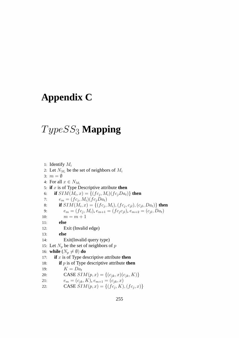
Appendix C

TypeSS3 Mapping

1: Identify Mi

2: Let NMibe the set of neighbors ofMi

3: m = ∅4: For allx ∈ NMi

5: if x is of Type Descriptive attributethen6: if SIM(Mi, x) = {(fcj,Mi)(fcjDat)} then7: em = (fcj, Mi)(fcjDat)8: if SIM(Mi, x) = {(fcj,Mi), (fcj, cjl), (cjl, Dat)} then9: em = (fcj,Mi), em+1 = (fcjcjl), em+2 = (cjl, Dat)

10: m = m + 111: else12: Exit (Invalid edge)13: else14: Exit(Invalid query type)15: Let Np be the set of neighbors ofp16: while (Np 6= ∅) do17: if x is of Type descriptive attributethen18: if p is of Type descriptive attributethen19: K = Dat

20: CASESIM(p, x) = {(cjk, x)(cjk, K)}21: em = (cjk, K), em+1 = (cjk, x)22: CASESIM(p, x) = {(fcj, K), (fcj, x)}

255

23: em = (fcj, K),em+1 = (fcj, x)24: CASESIM(p, x) = {(cjk, K), (cjn, x)}25: em(cjk, K) em+1 = (cjn, x) em+2 = (x, k)26: else27: Exit(Invalid query type)

256

Appendix D

TypeSM1 Mapping

1: Identify Mi

2: Let NMibe the set of neighbors ofMi {I}nitialising a variable to assign the

neighbour nodes ofMi

3: m = ∅4: For allx ∈ NMi

5: if x is of Type fundamental classthen6: if SIM(Mi, x) = (fcj,Mi) then7: em = (fcj, Mi)8: else9: Exit (Invalid edge)

10: else ifx is of type classthen11: if SIM(Mi, x) = {(fcj,Mi), (fcj, cjl)} then12: em = (fcj,Mi), em+1 = (fcjcjl)13: m = m + 114: else15: Exit (Invalid edge)16: else17: Exit(Invalid query type){P}revious steps test possible edges with a

measure node and edges are selected as perSIM function output.18: p = x19: m = m + 1

257

20: Let Np be the set of neighbors ofp {P}rocessing the remaining edges of thetree.

21: while (Np 6= ∅) do22: if x is of type classthen23: if p is of type fundamental classthen24: K = fcj

25: else26: K = ckl or K = cjl {T}he class can be from different lattices27: if SIM(p, x) = (K, cjk) then28: em = (K, cjk) {I}f K andcjk are from different lattices,em will be

a new edge that is added to the KB graph.29: else30: Exit(Invalid query type)31: else32: Exit(Invalid query type)33: m = m + 134: p = x35: Let Np be the set of neighbors ofp

258

Appendix E

TypeSM2 Mapping

1: Identify Mi

2: Let NMibe the set of neighbors ofMi {I}nitialising a variable to assign the

neighbour nodes ofMi

3: m = ∅4: For allx ∈ NMi

5: if x is of Type fundamental classthen6: if SIM(Mi, x) = (fcj,Mi) then7: em = (fcj, Mi)8: else9: Exit (Invalid edge)

10: else ifx is of type classthen11: if SIM(Mi, x) = {(fcj,Mi), (fcj, cjl)} then12: em = (fcj,Mi), em+1 = (fcjcjl)13: else ifx is of type descriptive attributethen14: if SIM(Mi, x) = {(fcj, Mi)(fcjDat)} then15: em = (fcj,Mi)(fcjDat)16: if SIM(Mi, x) = {(fcj,Mi), (fcj, cjl), (cjlDat)} then17: em = (fcj,Mi), em+1 = (fcjcjl) em+2 = (cjlDat)18: m = m + 119: else20: Exit (Invalid edge)21: else

259

22: Exit(Invalid query type){P}revious steps test possible edges witha measure node and edges are selected as perSIM function out-put.

23: p = x24: m = m + 125: Let Np be the set of neighbors ofp {P}rocessing the remaining edges of the

tree.26: while (Np 6= ∅) do27: if x is of type classthen28: CASEp is of type fundamental class29: K = fcj

30: CASEp is of type class31: K = cjl

32: CASEp is of type descriptive attribute33: K = Dat Go to Step 5234: CASEp none of the above three35: Exit(Invalid edge)36: if K = Dat then37: em = SIM(x, p)38: else ifSIM(p, x) = {(x, p), y} then39: em = SIM(x, p), em+1 = (x, y) em+2 = (y, p)40: y is a class butx andy are not the same.41: else42: em = SIM(K, cjk)43: if x is of type fundamental classthen44: CASEp is of type fundamental class45: K = fcj {x},p are not necessarily from the same classification46: CASEp is of type class47: K = ckl

48: CASEp is of type descriptive attribute49: K = Dat Go to Step 5250: CASEp none of the above three51: Exit(Invalid edge)52: if K = Dat then53: em = SIM(x, p)54: else ifSIM(p, x) = {(x, p), y} then55: em = SIM(x, p), em+1 = (x, y) em+2 = (y, p)56: y is a class butx andy are not the same.57: else58: em = SIM(K, cjk)

{T}esting different possible combinations of edges

260

59: if x is of Type descriptive attributethen60: CASEp is of type fundamental class61: K = fcj

62: CASEp is of type class63: K = cjl

64: CASEp is of type descriptive attribute65: K = Dat Go to Step 6866: CASEp is none of the above three type67: Exit(Invalid edge)68: if K = Dat then69: CASESIM(p, x) = {(cjk, x)(cjk, K)}70: em = (cjk, K), em+1 = (cjk, x)71: CASESIM(p, x) = {(fcj, K), (fcj, x)}72: em = (fcj, K),em+1 = (fcj, x)73: CASESIM(p, x) = {(cjk, K), (cjn, x)}74: em(cjk, K) em+1 = (cjn, x) em+2 = (x, k)75: else if em = SIM(K, cjk) then76: Where K is a class or fundamental class.77: else78: Exit(Invalid query type)79: m = m + 180: p = x81: Let Np be the set of neighbors ofp

261

Appendix F

TypeSM3 Mapping

1: Identify Mi

2: Let NMibe the set of neighbors ofMi {I}nitialising a variable to assign the

neighbour nodes ofMi

3: m = ∅4: For allx ∈ NMi

5: if x is of Type Descriptive attributethen6: if SIM(Mi, x) = {(fcj,Mi)(fcjDat)} then7: em = (fcj, Mi)(fcjDat)8: if SIM(Mi, x) = {(fcj,Mi), (fcj, cjl), (cjl, Dat)} then9: em = (fcj,Mi), em+1 = (fcjcjl), em+2 = (cjl, Dat)

10: m = m + 111: else12: Exit (Invalid edge)13: else14: Exit(Invalid query type)15: Let Np be the set of neighbors ofp16: while (Np 6= ∅) do17: if x is of Type descriptive attributethen18: if p is of Type descriptive attributethen19: K = Dat

20: CASESIM(p, x) = {(cjk, x)(cjk, K)}21: em = (cjk, K), em+1 = (cjk, x)

262

22: CASESIM(p, x) = {(fcj, K), (fcj, x)}23: em = (fcj, K), em+1 = (fcj, x)24: CASESIM(p, x) = {(cjk, K), (cjn, x)}25: em(cjk, K) em+1 = (cjn, x) em+2 = (x, k)26: CASESIM(p, x) = {(cjk, x)(cpq, K)}27: em = (cpq, K), em+1 = (cjk, x), em+2 = (x, k) {}(x, k) be the newly

added operational edge.28: CASESIM(p, x) = {(fcj, K), (fcp, x)}29: em = (fcj, K),em+1 = (fcp, x), em+2 = (x, k)30: else31: Exit(Invalid query type)

263

Appendix G

Intermediate Schema : An Example

A set of queries belong to various query types are illustrated here. Based on those

queries the intermediate schema is generated and shown in figure G.1.

Q1. Sales by Region

Q2 Total sales in quarter1 of year1997

Q3 Sales by product by package size

Q4 Sales by shop type

Q5 Sales by region by year

Q6 Average sales by supplier by week

Q7 Sales by clothing size by age

264

Q8 Average age of customers those who did a transaction for more than$100

Q9 Show the average sales

Q10 Show the stock-turn during the year1999

265

Figure G.1: An intermediate schema from case study

266