Bioresource Technology 102 (2011) 4688–4696

Contents lists available at ScienceDirect

Bioresource Technology

journal homepage: www.elsevier .com/locate /bior tech

Use of near infrared spectroscopy in online-monitoring of feeding substratequality in anaerobic digestion

H. Fabian Jacobi ⇑, Christian R. Moschner, Eberhard HartungInstitute of Agricultural Engineering, Christian-Albrechts-University Kiel, Max-Eyth-Str. 6, 24118 Kiel, Germany

a r t i c l e i n f o a b s t r a c t

Article history:Received 17 August 2010Received in revised form 12 January 2011Accepted 14 January 2011Available online 22 January 2011

Keywords:Anaerobic digestionBiogasMaize silageNear infrared spectroscopyOnline quality control

0960-8524/$ - see front matter � 2011 Elsevier Ltd. Adoi:10.1016/j.biortech.2011.01.035

⇑ Corresponding author. Tel.: +49 431 880 1435; faE-mail address: fjacobi@ilv.uni-kiel.de (H.F. Jacobi

In order to keep the anaerobic process stably and uniformly producing biogas it needs to be supplied witheither an even amount of substrate of stable quality or varying amounts according to variations in quality.Feeding amounts are usually adjusted manually as a reaction to changing rates of biogas production. Con-tinuous information about the actual substrate quality is not available and feedstuff analyses are costly.Aim of this study was to assess the feasibility of near infrared spectroscopic (NIRS) online monitoring ofsubstrate quality in order to find ways towards more exact control of biogas plant feeding. A NIRS sensorsystem was designed, constructed and calibrated for continuous monitoring of (RMSECV in brackets) drymatter (DM) (0.75 %fresh matter (FM)), volatile solids (0.74 %FM), crude fat (0.09 %FM), crude protein(0.22 %FM), crude fiber (1.50 %DM) and nitrogen-free extracts (0.93 %FM) of maize silage.

� 2011 Elsevier Ltd. All rights reserved.

1. Introduction

Biogas production by anaerobic digestion (AD) of biomass is ofgrowing importance in response to environmental and future en-ergy supply concerns. In Germany this sector has been particularlypromoted by legislative changes in the years 2000 and especially2004. By the end of the year 2010, about 5700 biogas plants havebeen established.

Modern biogas plants ferment liquid and/or solid substrates,mainly from agricultural sources. A typical liquid substrate is man-ure while the most abundant solid substrates are specificallygrown energy crops, such as maize and grass, which are beingstored as silages. More and more sugar beets are also being consid-ered a future energy crop. Monofermentation based solely onmaize silage has become very common. Furthermore organicwastes from different industries are used.

Agricultural substrates are relatively complex in compositionand – due to locally and temporarily diverging conditions ofgrowth and storage – varying in quality. Contrary to these varia-tions the biogas process itself calls for constant conditions regard-ing dosage and composition of the substrates. This can only beachieved by continuous and representative supervision of the sub-strates applying adequate sensors. To date control of substrate dos-age is mostly accomplished by regular automatic feeding based ongravimetrical or volumetrical assessment of substrate amounts,

ll rights reserved.

x: +49 431 880 4283.).

without substrate quality control. Changes in substrate quality,leading to altered biogas production, can therefore not be con-trolled in-time and have to be buffered by the mostly flexible gasstorage system until the plant operator reacts. Beyond this bufferthey lead to over- or underproduction of biogas, resulting in mon-etary losses. To date feeding strategies are adapted followingchanges in gas quality and quantity instead of reacting in advanceto changes and according to actual substrate quality.

Biomass composition for use as feedstuff for feedstock as wellas for biogas plants is usually described by Weender analysis(Jeroch et al., 1999), differentiating between dry matter (DM),crude ash, volatile solids (VS), crude protein (XP), crude lipids(XL), crude fiber (XF) and nitrogen-free extracts (NfE). Additionalinformation about the less digestible or indigestible fiber and lig-nin fractions can be provided by Van Soest analysis (Van Soest,1966).

Hence to date there is no tool for online supervision of substratethis study aimed at applying near infrared spectroscopy (NIRS) tothis end.

NIRS is being used in a wide range of applications in agricultureand has already been proposed as a process analytical tool for thesupervision of the anaerobic digestion process (Hansson et al.,2002; Jacobi et al., 2009; Lomborg et al., 2009; Nordberg et al.,2000) as well as for determination of manure composition (Doludet al., 2005; Saeys, 2006; Sorensen et al., 2007; Zimmermann,2009). Concerning the application for the monitoring of feedstuffquality it has been a standard analytical tool for a long period. Ini-tially and most commonly until today it is applied only to dried

H.F. Jacobi et al. / Bioresource Technology 102 (2011) 4688–4696 4689

samples, but at least since Abrams (1988) tried estimation of sev-eral parameters of fresh grass and legume silages it has been usedon undried samples in a couple of laboratory studies as well. Theresults from studies applying NIRS on fresh matter samples aimingat some of the Weender analysis parameters relevant for the bioga-sification process are cumulated in Table 1.

Measuring fresh, untreated silage samples containing plant par-ticles in the range of mm–cm calls for special care concerning therepresentativeness of the spectral measurements. Commonly vari-ous spectra of different fractions of the same sample are averagedin order to receive one representative spectrum. Reeves et al.(1989), found that calibrations of ground silages lead to superiorresults compared with unground samples. Similar results are pre-sented by Baker et al. (1994) and Gordon et al. (1998) using un-dried samples and by Lovett et al. (2005) with dried material.

Influences of sample, ambient and spectrometer temperature onNIR spectra are an issue well known to NIRS users and are well de-scribed in literature (Williams, 2001b). There are different ap-proaches to avoid temperature effects, most of which depend onknowledge of sample temperature. PLS-regression is supposed tobe able to overcome temperature effects. To this extend samplesfrom the complete range of temperatures to be expected for anapplication need to be included into the calibration data set (Hag-eman et al., 2005; Williams, 2001b). Since the aim of working in-process in real-life applications calls for measuring devices thatdo not need to interfere with the process, special treatment of thesubstances to be analyzed is to be avoided. This excludes comminu-tion as well as special temperature control. Therefore this studyaimed at evaluating the possibilities of silage characterization usingNIRS, avoiding special sample treatment or temperature control.

2. Methods

2.1. Linnau biogas plant

The Linnau biogas plant (Linnau, Schleswig–Holstein, Germany)is operated in the thermophilic temperature range (50–55 �C) andconsists of three process stages: primary and secondary heated fer-menter and an unheated repository for slurry storage. The plant is

Table 1Literature survey: Statistical parameters of reviewed NIR-calibrations of undried silages.

Para-meter Authors Range(nm) Regr.type

Pre-treatment

Deriva-tive

R2(%

DM Abrams (1988) smooth 1st 98Reeves et al. (1989) 1100–2500 MRP 99Reeves et al. (1989) 1100–2500 MRP 96Sorensen (2004) 400–2500 PLS SNVD 2nd 99Sorensen (2004) 400–2500 PLS SNVD 2nd 93Park et al. (2005) 400–2500 MPLS SNVD 1st 83(7Cozzolino et al. (2006) MPLS SNVD 2nd 85Liu and Han (2006) 1100–2500 PLS SC 1st 90Gibaud (2007) 960–1690 PLS MSC 98

XF Gibaud (2007) 960–1690 MPLS none 2nd 70

XP Reeves et al. (1989) 1100–2500 MRP 88Reeves et al. (1989) 1100–2500 MRP 83Sinnaeve et al. (1994) 400–2500 MPLS SNVD 2nd 97Cozzolino et al. (2006) MPLS SNVD 2nd 91Liu and Han (2006) 1100–2500 PLS SC 1st 82Gibaud (2007) 960–1690 MPLS SNVD 2nd 49

Italic and normal letters within one column mark differences within the calculation of avalues were calculated by the author if possible, otherwise left blank.

a Test set in brackets; A, alfalfa; CV, variation coefficient; DM, dry matter; FM, fresh maregression procedures; n, number of samples; PLS, partial least squares regression; R, ryesquare error of cross validation; RMSEP, root mean square error of prediction; RPD, ratioRMSECV or SD/RMSEP); SC, unspecified scatter correction; SD, standard deviation; SECV, stSEP); SNVD, standard normal variate with detrend; T, Trifolium; VS, volatile solids; XF,

fed only with maize silage. Cumulated input (and loading rates)varied during the observed period from 25–50 t FM d�1 (2.0–4.0 kg VS m�3 d�1) with an average of 37 t FM d�1 (3.0 kg VS m�3

d�1 calculated for the first two stages).

2.2. Near infrared spectroscopy

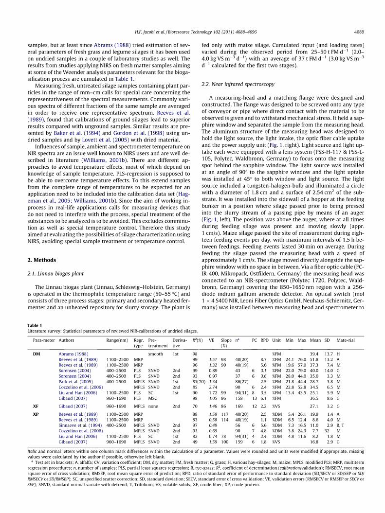
A measuring-head and a matching flange were designed andconstructed. The flange was designed to be screwed onto any typeof conveyor or pipe where direct contact with the material to beobserved is given and to withstand mechanical stress. It held a sap-phire window and separated the sample from the measuring head.The aluminum structure of the measuring head was designed tohold the light source, the light intake, the optic fiber cable uptakeand the power supply unit (Fig. 1, right). Light source and light up-take each were equipped with a lens system (PSS-H-117 & PSS-L-105, Polytec, Waldbronn, Germany) to focus onto the measuringspot behind the sapphire window. The light source was installedat an angle of 90� to the sapphire window and the light uptakewas installed at 45� to both window and light source. The lightsource included a tungsten-halogen-bulb and illuminated a circlewith a diameter of 1.8 cm and a surface of 2.54 cm2 of the sub-strate. It was installed into the sidewall of a hopper at the feedingbunker in a position where silage passed prior to being pressedinto the slurry stream of a passing pipe by means of an auger(Fig. 1, left). The position was above the auger, where at all timesduring feeding silage was present and moving slowly (appr.1 cm/s). Maize silage passed the site of measurement during eigh-teen feeding events per day, with maximum intervals of 1.5 h be-tween feedings. Feeding events lasted 30 min on average. Duringfeeding the silage passed the measuring head with a speed ofapproximately 1 cm/s. The silage moved directly alongside the sap-phire window with no space in between. Via a fiber optic cable (FC-IR-400, Mikropack, Ostfildern, Germany) the measuring head wasconnected to an NIR-spectrometer (Polytec 1720, Polytec, Wald-bronn, Germany) covering the 850–1650 nm region with a 256-diode indium gallium arsenide detector. An optical switch (mol1 � 4 S400 NIR, Leoni Fiber Optics GmbH, Neuhaus-Schiernitz, Ger-many) was installed between measuring head and spectrometer to

) VE Slope(%)

na PC RPD Unit Min Max Mean SD Mate-rial

%FM 39.4 13.7 H1.51 98 40(20) 8.7 %FM 24.1 76.0 51.8 13.2 A1.32 90 40(19) 5.6 %FM 19.6 57.0 37.3 7.4 M0.89 43 6 3.1 %FM 22.0 79.0 40.0 14.0 G0.97 37 6 3.6 %FM 28.0 44.0 35.0 3.3 M

0) 1.34 86(27) 2.5 %FM 21.8 44.4 28.7 3.8 M2.74 90 6 2.4 %FM 22.8 52.8 34.5 6.5 M1.72 99 94(31) 8 3.5 %FM 13.4 43.5 25.1 5.9 M1.05 96 158 13 6.1 %FM 36.5 8.6 G

1.46 86 169 12 2.2 %VS 27.1 3.2 G

1.59 117 40(20) 2.5 %DM 5.4 26.1 19.9 1.4 A0.58 114 40(19) 1.1 %DM 6.5 12.4 8.6 4.0 M0.49 56 6 5.6 %DM 7.3 16.5 11.0 2.9 R, T0.65 90 7 4.8 %DM 3.8 24.3 7.7 32 M0.74 78 94(31) 4 2.4 %DM 4.8 11.6 8.2 1.8 M1.59 100 159 6 1.8 %VS 16.8 2.9 G

parameter. Values were rounded and units were modified if appropriate, missing

tter; G, grass; H, various hay-silages; M, maize; MPLS, modified PLS; MRP, multiterm-grass; R2, coefficient of determination (calibration/validation); RMSECV, root meanof standard error of performance to standard deviation (SD/SECV or SD/SEP or SD/

andard error of cross validation; VE, validation errors (RMSECV or RMSEP or SECV orcrude fiber; XP, crude protein.

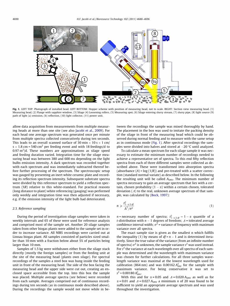
Fig. 1. LEFT TOP: Photograph of installed head. LEFT BOTTOM: Hopper scheme with position of measuring head, not to scale. RIGHT: Section view measuring head. (1)Measuring head, (2) Flange with sapphire window, (3) Silage (4) Loosening rollers, (5) Measuring spot, (6) Silage entering slurry stream, (7) slurry pipe, (8) light source (9)path of light (a) emission, (b) reflection, (10) light collector, (11) power unit.

4690 H.F. Jacobi et al. / Bioresource Technology 102 (2011) 4688–4696

allow data acquisition from measurements from multiple measur-ing heads at more than one site (see also Jacobi et al., 2009). Foreach head one average spectrum was generated once per minutefrom multiple spectra collected consecutively during ten seconds.This leads to an overall scanned surface of 30 min � 10 s � 1 cm/s � 1.8 cm = 540 cm2 per feeding event and with 18 feedings/d to0.97 m2/d. These numbers are approximations as silage speedand feeding duration varied. Integration time for the silage mea-suring head was between 380 and 600 ms depending on the lightbulbs emission intensity. A dark spectrum was recorded togetherwith each spectrum and was immediately subtracted thereof be-fore further processing of the spectrum. The spectroscopic setupwas gauged by presenting an inert white ceramic plate and record-ing its reflection spectrum intensity. Subsequent substrate spectrawere divided by this reference spectrum to yield a reflection spec-trum (%R) relative to this white-standard. For practical reasons(long distance to plant) white referencing (gauging) was performedonly weekly and integration time was then adjusted if necessary,e.g. if the emission intensity of the light bulb had deteriorated.

2.3. Reference sampling

During the period of investigation silage samples were taken inweekly intervals and 65 of these were used for reference analysisand comprised most of the sample set. Another 20 silage samplestaken from other biogas plants were added to the sample set in or-der to increase variance. All NIRS recordings were carried out atLinnau biogas plant. All samples consisted of particles sized smal-ler than 10 mm with a fraction below about 5% of particles beinglarger than 10 mm.

Samples of 1.5 kg were withdrawn either from the silage stackdirectly (mostly the foreign samples) or from the feeding unit atthe site of the measuring head (plants own silage). For spectralrecordings of the samples a steel box was hung inside the feedingunit in front of the measuring head. The side of the box facing themeasuring head and the upper side were cut out, creating an en-closed space accessible from the top. Into this box the samplewas placed. Multiple average spectra (see below) were recordedfrom each sample. Averages comprised out of continuous record-ings during ten seconds (as in continuous mode described above).During the recordings the sample would not move while in be-

tween the recordings the sample was mixed thoroughly by hand.The placement in the box was used to imitate the packing densityof the silage in front of the measuring head which could be ob-served during normal feeding and to measure with the same setupas in continuous mode (Fig. 1). After spectral recordings the sam-ples were divided into halves and stored at �20 �C until analyzed.

To calculate a mean spectrum for each silage sample it was nec-essary to estimate the minimum number of recordings needed toachieve a representative set of spectra. To this end fifty reflectionspectra from each of three different samples were collected as de-scribed above. These were transformed into absorption spectra(absorbance (A) = log (1/R)) and pre-treated with a scatter correc-tion (standard normal variate) as described below. In the followingthe resulting unit will be called ASNV. The minimum number ofspectra necessary to gain an average spectrum that lies with a cer-tain, chosen probability (1 � a) within a certain chosen, tolerateddeviation (D) to the real, unknown average spectrum of that sam-ple, was calculated by (Bock, 1997):

n Pt2

1�a=2;df

D2=r2ð1Þ

n = necessary number of spectra; t21�a=2;df ¼ 1� a quantile of a

t-distribution with n � 1 degrees of freedom; D = tolerated averageconfidence interval width; r2 = variance of frequency with maximumvariance over all spectra.

The exact sample size is given as the smallest n which fulfillsthe inequality (1) by means of df = n � 1 and is determined itera-tively. Since the true value of the variance (from an infinite numberof spectra) r2 is unknown, the sample variance s2 was used instead.For s2 the variance at each wavelength over all spectra of each sam-ple was determined and the wavelength with maximum variancewas chosen for further calculations. For all three samples wave-length variance was maximal at the lowest wavelength used forcalibration (864 nm) and was 0.00162 A2

SNV for the sample withmaximum variance. For being conservative it was set tos2 = 0.00180 A2

SNV.With this and for a = 0.05 and D = 0.020 ASNV as well as for

a = 0.01 and D = 0.027 ASNV a minimum n of 20 was found to besufficient to yield an appropriate average spectrum and was usedthroughout the investigation.

H.F. Jacobi et al. / Bioresource Technology 102 (2011) 4688–4696 4691

Additionally it should be mentioned that the average varianceover all wavelengths of the sample with maximum variance was0.00047 A2

SNV. This shows that mostly variance is significantly low-er than used here and correspondingly a much stricter D would bepossible. Also for comparison the value range of a complete stan-dardized average absorption spectrum of was �3 ASNV.

With this n and an observed surface of 2.54 cm2 per recording, atotal area of 20 � 2.54 � 50.8 cm2 was scanned for each sample.

2.4. Reference analysis

Frozen silage samples were sent to a commercial agriculturallaboratory and Weender (Jeroch et al., 1999) and Van Soest(1966) analyses were performed according to laboratory standardsas described in VDLUFA methods book volume III. Parameters fol-lowed by corresponding book sections in brackets as follows: DM(3.1), XA (8.1), XP (4.1.1), XF (6.1.1) and XL (5.1.1B); (VDLUFA,1976–2007). All analyses were made with dried material. NfE iscomposed of the residual components after subtraction of all otherabove mentioned values from DM.

2.5. Data acquisition

NIR spectra were constantly collected locally with an IBM-basedcomputer and later on transferred to a Linux-based PostgreSQLdata base. Feeding times, feeding amounts and sample analysis re-sults were also stored in the data base.

2.6. Multivariate data analysis

Average spectra of each sample were calculated and then ex-tracted from the data base for calibration. Spectra of each samplewere screened visually as plausibility check prior to averaging.Very abnormal spectra hinting to measurement or recording errorswere excluded from the data set. Visual screening excluded onlyvery few spectra and was preferred over an automatic filter, be-cause some samples were chosen for their extreme values andcame from maize-ear-silage that was added with a ratio of about1:50 to the daily ration of the plant. Automatic filtering (as de-scribed below) would have excluded these samples.

Sample outliers were excluded for the following reasons: (a)obvious deviation from the surrounding y-data and therefore beingjudged as outlier or analysis error and (b) for spectral inconsisten-cies of the average spectrum (this regards mostly to four samplesfrom the beginning of the measurement campaign, when problemswith a sapphire window were not resolved and lead to interfer-ences on the spectra) and (c) samples that were conspicuous inmore than one model or in model and principal component analy-

27 29 31 33 35 37 3927

29

31

33

35

37

39

VS p

redi

cted

VS measured

R²=91.61%

27 29 31 33 35 37 3927

29

31

33

35

37

39

VS p

redi

cted

VS measured

R²=89.62%

27 29 31 3327

29

31

33

35

37

39

VS p

redi

cted

VS me

R²=91.75%

27 29 31 3327

29

31

33

35

37

39

VS p

redi

cted

VS me

R²=87.26%

Fig. 2. Volatile solids calibration: Predicted vs. measured. Black (dots): Calibration datavalidation; RIGHT: Test set validation with extrapolation to extreme samples. (For interpweb version of this article.)

sis (PCA) (Tillmann, 1996) hinting to errors in either spectra acqui-sition or chemical analysis.

Chemometric multivariate data analysis for model developmentwas carried out using the Unscrambler� software versions 9.1 and9.6 (CAMO, Oslo, Norway). PCA (Hotelling, 1933; Naes et al., 2002)was applied to identify outliers.

Partial least square regression (PLS) was used to compute mod-els (Sjöström et al., 1983). For spectral pre-treatment the followingmethods were applied to the spectra: transformation from reflec-tion (%R) to absorption (A) (A = log(1/R)), standard normal variate(SNV) to evade stray light effects and Savitzky-Golay derivativesin order to evade parallel displacement, (Tillmann, 1996); center-ing and scaling to unit variance by division of each spectral valueby the standard deviation of all values at each frequency. Full crossand test set validation were applied in order to evaluate model per-formance (Kessler, 2007).

For selection of the samples for the calibration set a clusteranalysis using the pretreated spectra was done. In 20 iterationssamples were divided into 20 clusters applying Kendall’s Tau dis-tance measurements as implemented in the Unscrambler� soft-ware. Samples were then sorted by clusters and within theclusters by VS. One to three samples were selected from each clus-ter for the calibration set whereas the remaining samples were as-signed to the validation set.

As it is rather impossible to control temperatures (meaningambient, sample and measuring head temperature) on site, sam-ples were measured under the actual (temperature-) conditions.The inclusion of samples measured over the whole range of tem-peratures expected is described as one method to overcome tem-perature-dependent deterioration of PLS-models (Hageman et al.,2005) and was therefore the method of choice.

Model quality was judged by the following parameters: thenumber of principal components (PC); coefficient of determina-tion (R2); the root mean square error of cross validation(RMSECV), of calibration (RMSEC) and of prediction from testset validation (RMSEP) (Kessler, 2007). The slope of the regres-sion line and the residual predictive value (RPD) being the ratioof standard deviation (SD) and RMSECV (Williams, 2001a) werealso considered. Furthermore the performance for the predictionof time series was taken into account. Hereby the comparison ofthe calculated time series with the reference values’ course withemphasis on sensitivity to changes over time (as in Fig. 3) wereassessed.

2.7. Time series

All spectra recorded during feeding events – i.e. while silagewas passing the measuring head – were extracted from the data

35 37 39asured

35 37 39asured

27 32 37 42 47 5227

32

37

42

47

52

VS p

redi

cted

VS measured

R²=91.75%

27 32 37 42 47 5227

32

37

42

47

52

VS p

redi

cted

VS measured

R²=97.27%

. Red/grey (circles): Validation data. LEFT: Full cross validation; MIDDLE: Test setretation of the references to color in this figure legend, the reader is referred to the

2628303234363840

VS N

IRS

(% F

M)

2628303234363840

VS re

fere

nce

(% F

M)

18

20

22

24

26

28

NfE

NIR

S (%

FM

)

18

20

22

24

26

28

NfE

refe

renc

e (%

FM

)

13

15

17

19

21

dXF

NIR

S (%

DM

)

13

15

17

19

21

dXF

refe

renc

e (%

DM

)

1.6

2

2.4

2.8

3.2

XP N

IRS

(% F

M)

1.6

2

2.4

2.8

3.2

XP re

fere

nce

(% F

M)

0.6

0.8

1

1.2

1.4

XL N

IRS

(% F

M)

02−Dec01−Jan01−Feb02−Mar02−Apr02−May02−Jun 02−Jul 02−Aug01−Sep02−Oct01−Nov02−Dec01−Jan0.6

0.8

1

1.2

1.4

XL re

fere

nce

(% F

M)

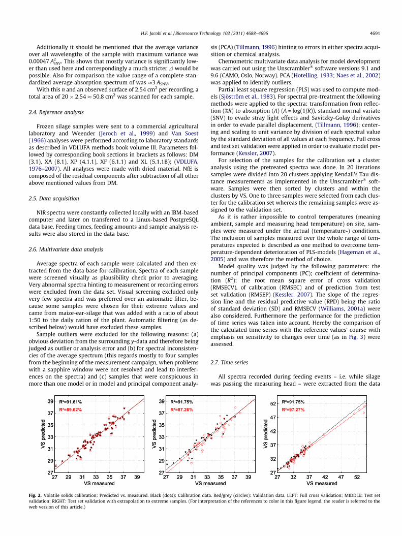
Fig. 3. Time series of chemical properties of input substrate (maize silage). Small dots: 8 h-averages of predicted values. Circles: reference sample laboratory values.VS = volatile solids, NfE = nitrogen free extract, dXF = crude fiber, XP = crude protein, XL = crude lipids.

4692 H.F. Jacobi et al. / Bioresource Technology 102 (2011) 4688–4696

base. Spectra were excluded, when not fitting into the range nor-mally observed (40–95 %R) at 1069 nm in order to withhold invalidspectra from the prediction. For prediction only full-cross validatedmodels from the full sample set (only excluding outliers and for theA-set extreme samples) were chosen. The reason for not choosingthe calibration models from test set validation is the low numberof samples in the calibration data set (31–35), which could leadto more sample dependence of the models and therefore tooverfitting.

The chosen PLS-models (Table 4 in bold type) were then appliedto the resulting set of approximately 137,000 spectra, yielding ex-post time series of concentration values for the entire period ofinvestigation.

3. Results and discussion

3.1. Sample data description

Silage reference samples were analyzed as described above.Analyte concentrations are within the expected ranges for maizesilage, although the ranges are rather narrow; descriptive statisticsare shown in Table 2. Concentrations are hardly normally distrib-uted for all parameters and XP is skewed towards lower concentra-tion values (data not shown). Apart from the majority, five samplesshow extreme values as they originate from additionally fed silagemade only from maize-cobs and cob-leaves (maize-ear-silage) orblending of maize-ear-silage with normal silage. These samples’

Table 2Reference analysis statistics of maize silage samples used for calibration.

Set Analyte Unit Min Max SD Mean Median

A DM %FM 28.30 39.00 2.35 34.14 34.00B DM %FM 27.30 55.50 4.59 34.99 34.20A VS %FM 27.17 37.80 2.32 33.01 32.83B VS %FM 26.20 54.40 4.61 33.80 33.10A NfE %FM 17.31 27.20 1.96 23.42 23.30B NfE %FM 17.31 42.70 4.05 24.23 23.60B dXF %DM 8.36 22.90 2.37 17.58 17.90A XP %FM 2.05 3.40 0.31 2.47 2.39B XP %FM 2.05 4.11 0.45 2.54 2.40A XL %FM 0.55 1.13 0.12 0.94 0.96B XL %FM 0.55 1.87 0.20 0.97 0.96

A: excluding five extreme samples; B: all samples; FM, fresh matter, DM, drymatter, VS, volatile solids, NfE, nitrogen free extract, dXF, crude fiber based on drymatter, XP, crude protein, XL, crude lipids;

Table 3Parameter cross-correlation: Coefficient of determination of different quality param-eters vs. volatile solids (VS) based on dry-matter (DM) and fresh-matter (FM)concentrations.

R2 (%) Set NfE XF XL XP dNfE dXF dXL dXP

VS A 95.67 21.61 47.53 39.80 20.48 13.94 4.13 0.41VS B 98.74 0.00 82.22 70.81 69.43 60.52 26.60 0.00

R2-values calculated from two different data sets: A: excluding four extreme sam-ples; B: all samples; all parameters in %FM unless preceded by ‘‘d’’ indicating %DMas unit;

H.F. Jacobi et al. / Bioresource Technology 102 (2011) 4688–4696 4693

reference analysis values deviated by more than 1.5 (one blendedsample) and up to 5.5 standard deviations from the correspondingmean value (see Fig. 2, right). In- and exclusion of these sampleswas used to examine, whether they could aid calibration andwhether extrapolation was possible from models calculated byusing only regular samples. Table 2 describes the sample set with(B) and without (A) the inclusion of extreme samples.

Within the reference values correlations to DM and VS were ob-served. In Table 3 the coefficients of determination for such corre-lations are given. For NfE (%FM) these are very high, whereas for allother parameters and bases (%FM or %DM) they vary greatly. Gen-erally they are higher for B-models, as they include the extremesamples, with the exception of XF.

Table 4Statistical parameters of PLS-models.

Set Analyte

Full cross validation

PCs n Slope (%) Offset RPD R2 (%)

A DM 4 72 91.3 2.95 3.10 89.6B DM 2 79 99.8 0.14 4.92 96.0B DM 4 79 96.1 1.35 5.13 96.2A VS 4 72 91.3 2.87 3.10 89.6B VS 2 78 94.9 1.68 4.74 95.6B VS 4 78 96.2 1.27 5.24 96.4A NfE 3 73 78.8 4.95 2.10 77.2B NfE 2 77 94.9 1.21 4.23 94.5B NfE 3 77 94.6 1.31 4.49 95.0B dXF 3 79 63.6 6.42 1.57 59.8A XP 3 75 54.4 1.12 1.42 50.8B XP 3 79 77.3 0.57 2.02 75.7A XL 4 74 55.7 0.41 1.44 51.8B XL 4 78 83.2 0.16 2.24 80.1

Model parameters for full cross validation (FCV) using all samples and test set validation (was used. A: excluding five extreme samples; B: all samples; italics: B-model with suggesNfE, nitrogen free extract, dXF, crude fiber based on dry matter, XP, crude protein, XL, crudprediction; bold letters: models selected for time series plots (Fig. 3), units: all values in

3.2. Multivariate data analysis/NIRS-calibration

Various combinations of wavelength range selections, data pre-treatments and sample exclusions were tried out in order to opti-mize the models. The best models were achieved with full rangeabsorption spectra. These were converted into first derivative spec-tra and smoothed, applying a 2nd order polynomial smoothing(Savitzky and Golay, 1964) over 13 data points (=38.1 ± 1.1 nm). Fi-nally spectra were SNV-normalized and centered and scaled tovariance.

Test set sample selection yielded calibration sets consisting of33 (A-set) and 35 (B-set) samples. Test set calibration yielded dif-ferent suggestions for the optimal number of PCs as full-cross val-idation (FCV) did. For statistics of test set calibration and validationthe number of PCs suggested by FCV was applied (Table 4). This ap-proach was chosen to allow better comparison between the meth-ods. Also, because of the low sample numbers, the test setcalibrations are likely subject to overfitting as mentioned above.

Calibration was tried on both DM- and FM-basis for all param-eters except VS. FM-based calibrations generally resulted in muchbetter models than DM-based calibrations especially for NfE, butexcept for crude fiber. Williams, 2001a states that calibration ofmaize on a constant moisture basis (like %DM) can become prob-lematic, when samples extend over a moisture range larger then3–4%. On the contrary all (of the few) studies working with freshsilages found in the literature calibrated XF and XP against DM-based analyte concentrations, while also working with moistureranges well above 4% (see Table 1).

Only FM-based values are of interest for the practical plantoperation, as feeding takes place by weight of fresh material.Therefore calibrations directly based on FM should be of advan-tage. The counting back from DM-based prediction values to FM-based prediction values is possible through multiplication withthe corresponding predicted DM-value. But it bears the disadvan-tage of the addition of prediction errors of the two models.

For comparison of the chosen models and validation techniques,their performance parameters are listed in Table 4. Exemplarilyplots of predicted vs. measured values are displayed in Fig. 2. Inthe case of DM, VS and NfE the suggested optimal number of PCsis differing between A- and B-models. When using the suggestednumber of PCs, models excluding the five extreme samples (A)show generally poorer performance parameters than those includ-ing them (B). This is also true, when applying the same number of

Test set validation

Calibration Validation

RMSE CV n R2 (%) RMSE C n R2 (%) RMSE P

0.75 32 91.6 0.69 40 86.6 0.911.03 35 97.7 0.81 45 94.2 1.210.89 35 98.1 0.74 45 95.7 1.060.74 32 91.7 0.68 40 87.3 0.880.97 34 93.9 1.03 44 90.3 1.560.87 34 97.5 0.65 44 96.3 0.970.93 31 83.1 0.72 42 70.2 1.160.95 32 93.0 0.95 44 90.5 1.360.90 32 95.8 0.73 44 95.3 0.951.50 35 66.5 1.40 44 62.2 1.430.22 33 61.1 0.18 42 50.2 0.240.22 35 82.5 0.18 44 71.6 0.250.09 32 63.7 0.07 42 41.7 0.090.09 35 89.9 0.08 43 70.3 0.09

TSV) using selected subsets. For TSV the number of PCs suggested for the FCV-modelted number of PCs for A-model; FM, fresh matter, DM, dry matter, VS, volatile solids,e lipids, RMSE C, root mean square error of calibration / CV, of cross validation / P, of%FM except dXF in %DM;

25

27

29

31

33

35

37

VS

(g

/kg

FM

) n

o a

vera

ge

25

27

29

31

33

35

37

VS

(g

/kg

FM

) 4h

−ave

rag

e

29

31

33

VS

(g

/kg

FM

) 8h

−ave

rag

e

02 03 04 05 06 07 08 09 10 11 12 13 14 15 16 17 18 19 2029

31

33

VS

(g

/kg

FM

) 24

h−a

vera

ge

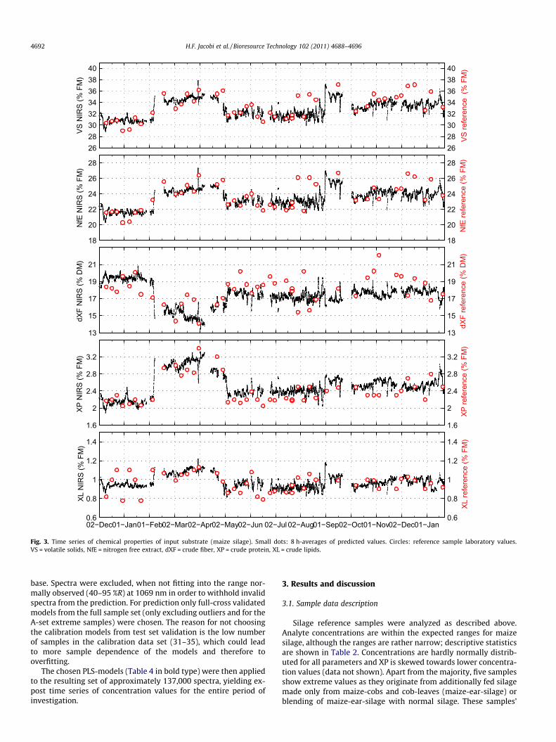
Fig. 4. Variation in and smoothing of the data: Time series of VS from January 1st–20th. TOP: raw prediction results (black), 4 h-average (red/grey). BOTTOM: 8 h-average(black), 24 h-average (red/grey). VS = volatile solids. (For interpretation of the references to color in this figure legend, the reader is referred to the web version of this article.)

4694 H.F. Jacobi et al. / Bioresource Technology 102 (2011) 4688–4696

PCs for the B-models as are suggested for the corresponding A-models (Table 4). In this case B-models generally improve, whereasfor DM and VS parameters improve more than for NfE. Test set val-idation yields poorer or the same validation results as full crossvalidation, except for dXF. Generally no major changes are ob-served between validation methods (see Table 4 and Fig. 2).

To test extrapolation capability of the A-models, the extremesamples were included into the validation set. The VS-A-modelshowed to be well capable of correctly predicting these samplesreference values, although they are by far out of the models range.This is displayed in the right plot of Fig. 2. It is also true for DM andXL, whereas with NfE and XP models this extrapolation leads toslope deterioration and a high bias of validation statistics.

Compared to other studies all presented models need only fewPCs in order to describe the variables’ variances to the optimallypossible extend. The RMSECVs are within (XP) or below (DM anddXF) the results found in the literature in Table 1. For comparisonwith the literature values the RMSECV (%FM) of XP was convertedto the unit %DM by division by the mean value for dry matter (Ta-ble 2) (for the A-set that results in an RMSECV of 0.64 %DM). RPDsare also within the results of other studies, although especially forthe A-set partially on a very low level. Ranges for the RPD-interpre-tation, proposed by Williams, 2001a, indicate that values below 2.4stand for very poor model performance, values between 2.4 and 3.0are good enough for rough screening, only values above allowproper screening. The difference in RPD values between the A-and B-models is to be attributed to the dramatic change in rangesand therefore in SD-values when including the extreme samples.When applied to the constantly collected silage spectra in orderto produce time series, the A-set models performed better thanthe B-set models. This is also addressed in Section 3.3.

As water is the major constituent of the silage its variationstrongly affects the FM-based concentration values of all otherconstituents. Therefore it cannot be ruled out that a correlationof constituents to water content (and thereby to VS, see Table 3)has a positive influence on the calculation of PLS-models of theseconstituents. However, for the practical application there is no dif-ference whether a model functions based on the actual detection of

a constituent or through cross-correlation to another, detectableconstituent as long as this correlation is consistent.

Expectably the presented models are not able to cope withchemical analysis, but for the intended purpose of detectingchanges in substrate quality they seem feasible to use.

Besides the presented parameters lignocellulosic fractions ofthe silage samples were also determined, but calibration of thesedid not yield useful models (data not shown).

3.3. Time series

Time series yielding the course of concentration values for allfour parameters were developed in order to verify suitability ofthe models to follow quality changes over time. This was achievedby the application of the PLS-models to the spectra continuouslyrecorded during feeding events. The resulting, calculated coursesof the silage constituents are shown in Fig. 3 over the time of theinvestigation period. The parameters are given in the units accord-ing to the chosen models (all in %FM except XF in %DM).

Because of the mode of sample presentation each single spec-trum cannot be seen as a representative spectrum for the current,over-all quality of silage entering the process. Therefore the pre-dicted values were averaged over a period of 8 h (see also Fig. 4and corresponding description below).

All predicted values stay within the range of the reference dataand follow the course of silage quality indicated by the referencevalues. Thereby it has to be noted that a particular reference sam-ple is not necessarily representative for the time point or period itwas drawn. Therefore the reliability of predicted values cannot bejudged solely by the closeness of these predicted values to nearbyreference data points, but has to be judged by whether the generalcourses of reference and predicted values fit together.

All analytes given in %FM show a similar course. This is owed tothe fact that the variation in the analytes’ concentrations is domi-nated by the variation of the amount of water in the silage. Modeldevelopment for crude fiber was difficult and yielded only a modelbased on the B-set and on DM-basis. Hence the time series for

VS (%FM)

-1.0

-0.5

0.0

0.5

1.0

dXF (%VS)

-0.6

-0.4

-0.2

0.0

0.2

0.4

0.6

NfE (%FM)-0.8

-0.6

-0.4

-0.2

0.0

0.2

0.4

0.6

0.8

XL (%FM)-0.06

-0.04

-0.02

0.00

0.02

0.04

0.06

XP (%FM)

-0.10

-0.05

0.00

0.05

0.10

32.92 17.4823.51 0.98 2.22

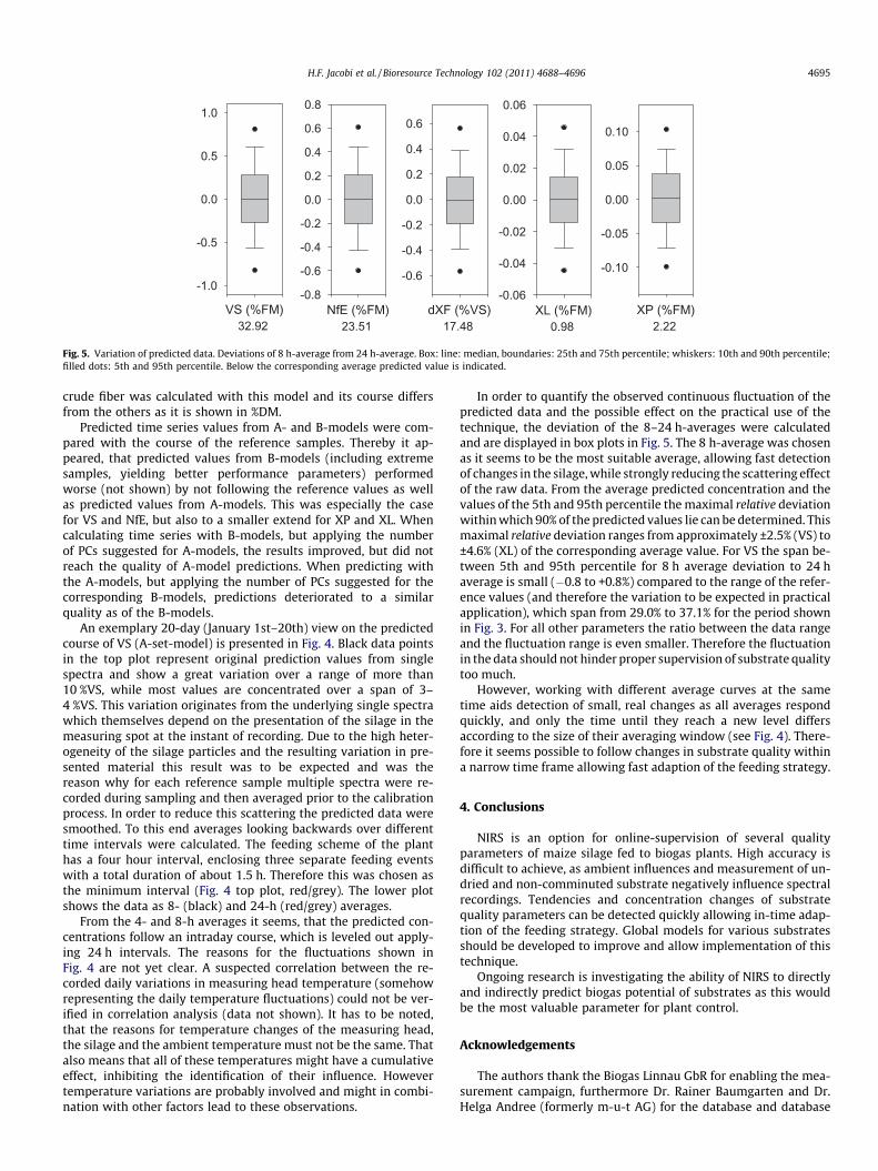
Fig. 5. Variation of predicted data. Deviations of 8 h-average from 24 h-average. Box: line: median, boundaries: 25th and 75th percentile; whiskers: 10th and 90th percentile;filled dots: 5th and 95th percentile. Below the corresponding average predicted value is indicated.

H.F. Jacobi et al. / Bioresource Technology 102 (2011) 4688–4696 4695

crude fiber was calculated with this model and its course differsfrom the others as it is shown in %DM.

Predicted time series values from A- and B-models were com-pared with the course of the reference samples. Thereby it ap-peared, that predicted values from B-models (including extremesamples, yielding better performance parameters) performedworse (not shown) by not following the reference values as wellas predicted values from A-models. This was especially the casefor VS and NfE, but also to a smaller extend for XP and XL. Whencalculating time series with B-models, but applying the numberof PCs suggested for A-models, the results improved, but did notreach the quality of A-model predictions. When predicting withthe A-models, but applying the number of PCs suggested for thecorresponding B-models, predictions deteriorated to a similarquality as of the B-models.

An exemplary 20-day (January 1st–20th) view on the predictedcourse of VS (A-set-model) is presented in Fig. 4. Black data pointsin the top plot represent original prediction values from singlespectra and show a great variation over a range of more than10 %VS, while most values are concentrated over a span of 3–4 %VS. This variation originates from the underlying single spectrawhich themselves depend on the presentation of the silage in themeasuring spot at the instant of recording. Due to the high heter-ogeneity of the silage particles and the resulting variation in pre-sented material this result was to be expected and was thereason why for each reference sample multiple spectra were re-corded during sampling and then averaged prior to the calibrationprocess. In order to reduce this scattering the predicted data weresmoothed. To this end averages looking backwards over differenttime intervals were calculated. The feeding scheme of the planthas a four hour interval, enclosing three separate feeding eventswith a total duration of about 1.5 h. Therefore this was chosen asthe minimum interval (Fig. 4 top plot, red/grey). The lower plotshows the data as 8- (black) and 24-h (red/grey) averages.

From the 4- and 8-h averages it seems, that the predicted con-centrations follow an intraday course, which is leveled out apply-ing 24 h intervals. The reasons for the fluctuations shown inFig. 4 are not yet clear. A suspected correlation between the re-corded daily variations in measuring head temperature (somehowrepresenting the daily temperature fluctuations) could not be ver-ified in correlation analysis (data not shown). It has to be noted,that the reasons for temperature changes of the measuring head,the silage and the ambient temperature must not be the same. Thatalso means that all of these temperatures might have a cumulativeeffect, inhibiting the identification of their influence. Howevertemperature variations are probably involved and might in combi-nation with other factors lead to these observations.

In order to quantify the observed continuous fluctuation of thepredicted data and the possible effect on the practical use of thetechnique, the deviation of the 8–24 h-averages were calculatedand are displayed in box plots in Fig. 5. The 8 h-average was chosenas it seems to be the most suitable average, allowing fast detectionof changes in the silage, while strongly reducing the scattering effectof the raw data. From the average predicted concentration and thevalues of the 5th and 95th percentile the maximal relative deviationwithin which 90% of the predicted values lie can be determined. Thismaximal relative deviation ranges from approximately ±2.5% (VS) to±4.6% (XL) of the corresponding average value. For VS the span be-tween 5th and 95th percentile for 8 h average deviation to 24 haverage is small (�0.8 to +0.8%) compared to the range of the refer-ence values (and therefore the variation to be expected in practicalapplication), which span from 29.0% to 37.1% for the period shownin Fig. 3. For all other parameters the ratio between the data rangeand the fluctuation range is even smaller. Therefore the fluctuationin the data should not hinder proper supervision of substrate qualitytoo much.

However, working with different average curves at the sametime aids detection of small, real changes as all averages respondquickly, and only the time until they reach a new level differsaccording to the size of their averaging window (see Fig. 4). There-fore it seems possible to follow changes in substrate quality withina narrow time frame allowing fast adaption of the feeding strategy.

4. Conclusions

NIRS is an option for online-supervision of several qualityparameters of maize silage fed to biogas plants. High accuracy isdifficult to achieve, as ambient influences and measurement of un-dried and non-comminuted substrate negatively influence spectralrecordings. Tendencies and concentration changes of substratequality parameters can be detected quickly allowing in-time adap-tion of the feeding strategy. Global models for various substratesshould be developed to improve and allow implementation of thistechnique.

Ongoing research is investigating the ability of NIRS to directlyand indirectly predict biogas potential of substrates as this wouldbe the most valuable parameter for plant control.

Acknowledgements

The authors thank the Biogas Linnau GbR for enabling the mea-surement campaign, furthermore Dr. Rainer Baumgarten and Dr.Helga Andree (formerly m-u-t AG) for the database and database

4696 H.F. Jacobi et al. / Bioresource Technology 102 (2011) 4688–4696

queries as well as Christoph Appel for software development andKerstin Otte, Christoph Martens and Jan Soltau for their samplingefforts. This study was funded by the German Federal Ministry ofFood, Agriculture and Consumer Protection (Grant 22003606)and Biogas Linnau GbR. The authors are responsible for the contentof this publication.

References

Abrams, S.M., 1988. Potential of near infrared reflectance spectroscopy for analysisof silage composition. J. Dairy Sci., 1955–1959.

Baker, C.W., Givens, D.I., Deaville, E.R., 1994. Prediction of organic-matterdigestibility in-vivo of grass-silage by near-infrared reflectance spectroscopy– effect of calibration method, residual moisture and particle-size. Anim. FeedSci. Technol. 50, 17–26.

Bock, J., 1997. Bestimmung des Stichprobenumfangs: Für biologische Experimenteund kontrollierte klinische Studien. (engl.: Determination of sample size: Forbiological experiments and controlled clinical studies.). Oldenbourg, München.

Cozzolino, D., Fassio, A., Fernandez, E., Restaino, E., La Manna, A., 2006.Measurement of chemical composition in wet whole maize silage by visibleand near infrared reflectance spectroscopy. Anim. Feed Sci. Technol. 129, 329–336.

Dolud, M., Andree, H., Hügle, T., 2005. Rapid analysis of liquid hog manure usingnear-infrared spectroscopy in flowing condition. In: Cox, S. (Ed.), PrecisionLivestock Farming ’05. Wageningen Academic Publishers, Wageningen, pp.115–122.

Gibaud, H., 2007. Nahinfrarotspektroskopische Erfassung und Charakterisierung dernutritiven und fermentativen Qualität von Grassilage im ungetrocknetenZustand. (engl.: Determination and characterization of nutritive andfermentative quality of undried grass silages with near-infraredspectroscopy). Fakultät für Agrarwissenschaften der Georg-August-UniversitätGöttingen, Göttingen.

Gordon, F.J., Cooper, K.M., Park, R.S., Steen, R.W.J., 1998. The prediction of intakepotential and organic matter digestibility of grass silages by near infraredspectroscopy analysis of undried samples. Anim. Feed Sci. Technol. 70, 339–351.

Hageman, J.A., Westerhuis, J.A., Smilde, A.K., 2005. Temperature robust multivariatecalibration: an overview of methods for dealing with temperature influences onnear infrared spectra. J. Near Infrared Spectrosc. 13, 53–62.

Hansson, M., Nordberg, A., Sundh, I., Mathisen, B., 2002. Early warning ofdisturbances in a laboratory-scale MSW biogas process. Water Sci. Technol.45, 255–260.

Hotelling, H., 1933. Analysis of a complex of statistical variables into principalcomponents. J. Ed. Psych. 24, 417–441.

Jacobi, H.F., Moschner, C.R., Hartung, E., 2009. Use of near infrared spectroscopy inmonitoring of volatile fatty acids in anaerobic digestion. Water Sci. Technol. 60,339–346.

Jeroch, H., Drochner, W., Simon, O., 1999. Ernährung landwirtschaftlicher Nutztiere(engl.: Nutrition of livestock). Eugen Ulmer, Stuttgart.

Kessler, W., 2007. Multivariate Datenanalyse für die Pharma-, Bio- undProzessanalytik (Multivariate data analysis for pharma-, bio- and processanalytics). Wiley-VCH, Weinheim.

Liu, X., Han, L.J., 2006. Prediction of chemical parameters in maize silage by nearinfrared reflectance spectroscopy. J. Near Infrared Spectrosc. 14, 333–339.

Lomborg, C.J., Holm-Nielsen, J.B., Oleskowicz-Popiel, P., Esbensen, K.H., 2009. Nearinfrared and acoustic chemometrics monitoring of volatile fatty acids and drymatter during co-digestion of manure and maize silage. Bioresour. Technol. 100,1711–1719.

Lovett, D.K., Deaville, E.R., Givens, D.I., Finlay, M., Owen, E., 2005. Near infraredreflectance spectroscopy (NIRS) to predict biological parameters of maizesilage: effects of particle comminution, oven drying temperature and thepresence of residual moisture. Anim. Feed Sci. Technol. 120, 323–332.

Naes, T., Isaaksson, T., Fearn, T., Davies, T., 2002. A Userfriendly Guide toMultivariate Calibration and Classification. NIR publications, Chichester.

Nordberg, A., Hansson, M., Sundh, I., Nordkvist, E., Carlsson, H., Mathisen, B., 2000.Monitoring of a biogas process using electronic gas sensors and near-infraredspectroscopy (NIR). Water Sci. Technol. 41, 1–8.

Park, H.S., Lee, J.K., Fike, J.H., Kim, D.A., Ko, M.S., Ha, J.K., 2005. Effect of samplepreparation on prediction of fermentation quality of maize silages by nearinfrared reflectance spectroscopy. Asian–Aust. J. Anim. Sci. 18, 643–648.

Reeves, J.B., Blosser, T.H., Colenbrander, V.F., 1989. Near-infrared reflectancespectroscopy for analyzing undried silage. J. Dairy Sci. 72, 79–88.

Saeys, W., 2006. Technical Tools for the Optimal Use of Animal Manure as aFertiliser Bio-ingenieurswetenschappen. Katholieke Universiteit Leuven,Leuven. pp. 215.

Savitzky, A., Golay, M.J.E., 1964. Smoothing + differentiation of data by simplifiedleast squares procedures. Anal. Chem. 36, 1627–1639.

Sinnaeve, G., Dardenne, P., Agneessens, R., 1994. Global or local? A choice for NIRcalibrations in analyses of forage quality. J. Near Infrared Spectrosc. 2, 163–175.

Sjöström, M., Wold, S., Lindberg, W., Persson, J.-Å., Martens, H., 1983. A multivariatecalibration problem in analytical chemistry solved by partial least-squaresmodels in latent variables. Anal. Chim. Acta 150, 61–70.

Sorensen, L.K., 2004. Prediction of fermentation parameters in grass and corn silageby near infrared spectroscopy. J. Dairy Sci. 87, 3826–3835.

Sorensen, L.K., Sorensen, P., Birkmose, T.S., 2007. Application of reflectance nearinfrared spectroscopy for animal slurry analyses. Soil Sci. Soc. Am. J. 71, 1398–1405.

Tillmann, P., 1996. Kalibrationsentwicklung für NIRS-Geräte: eine Einführung(Calibration development for NIRS-devices: an introduction). Cuvillier,Göttingen.

Van Soest, P.J., 1966. Nonnutritive residues: A system of analyses for thereplacement of crude fibre Seventy-ninth Annual Meeting assoc. of OfficialAgr. Chem., pp. 546–551.

VDLUFA, 1976–2007. Band III: 1.-7- Ergänzung. Die chemische Untersuchung vonFuttermitteln. (engl.: Chemical Analysis of animal feeds.) VDLUFA, Speyer.

Williams, P.C., 2001a. Implementation of near-infrared technology. In: Williams, P.,Norris, K. (Eds.), Near-Infrared Technology in the Agricultural and FoodIndustries, 2nd ed. American Association of Cereal Chemists, St. Paul, pp.145–169.

Williams, P.C., 2001b. Variables affecting near-infrared spectroscopic analysis. In:Williams, P., Norris, K. (Eds.), Near-Infrared Technology in the Agricultural andFood Industries, 2nd ed. American Association of Cereal Chemists, St. Paul, pp.171–198.

Zimmermann, A., 2009. Entwicklung und Grundlagenuntersuchungen einerkontinuierlichen Messmethode zur nährstoffgesteuerten Ausbringung vonFlüssigmist. (engl.: Development and basic investigations of a continuousmeasuring method for nutrient-based application of liquid manure). Institut fürLandwirtschaftliche Verfahrenstechnik. Christian-Albrechts-Universität zu Kiel,Kiel. pp. 180.