use of multiple models and qualitative knowledge for on-line
TRANSCRIPT

Use of Multiple Models and Qualitative Knowledge for On-line
Moving Horizon Disturbance Estimation and Fault Diagnosis
Edward P.Gatzke, Francis J. Doyle III∗
Department of Chemical Engineering
University of Delaware
Newark, DE 19716
Abstract
An integrated fault detection, fault isolation, and parameter estimation technique is presented in this
paper. Process model parameters are treated as disturbances that dynamically affect the process outputs.
A moving horizon estimation technique minimizes the error between process and model measurements
over a finite horizon by calculating model parameter values across the estimation horizon. To implement
qualitative process knowledge, this minimization is constrained such that only a limited number of
different faults (parameters) may change during a specific horizon window. Multiple linear models are
used to capture nonlinear process characteristics such as asymmetric response, variable dynamics, and
changing gains. Problems of solution multiplicity and computational time are addressed. Results from
a nonlinear chemical reactor simulation are presented.
Keywords: Moving Horizon Estimation, Multiple Linear Models, Mixed Integer Program-
ming, Disturbance Estimation
∗Author to whom correspondence should be addressed: [email protected]
1
1 Introduction
Fault detection is a critical problem for the chemical process industries. In order to ensure both
safe operations and quality production, process faults must be detected and isolated. If a fault is
considered as a continuous disturbance that disrupts a process, the extent of the disturbance should
be estimated in order for corrective actions to be taken. Using model-based approaches, parameter
estimation techniques can provide accurate estimates for the disturbance levels of a process. Linear
estimation techniques can prove inadequate in cases involving nonlinear systems. On the other
hand, nonlinear estimation techniques can quickly become intractable for problems of moderate
size. Industrial systems typically have many unmeasured disturbances which can and should be
estimated for use in control strategies. Excessive change in an unmeasured disturbance can be
considered a system fault. Such faults may not be a catastrophic process event, but rather a change
in the system that adversely affects the system properties. A method for quickly and accurately
detecting faults and estimating parameter values is desirable to keep processes running safely and
on-target. The integrated problem of fault detection, isolation, and estimation for nonlinear systems
incorporates concepts from the fields of fault diagnosis, state estimation, and nonlinear modeling.
Fault detection and isolation has become an important topic for chemical engineers attempting
to minimize process down time and prevent industrial accidents. A typical approach for fault
detection and diagnosis is to compare the process model outputs and actual process values [1, 32,
33]. Such residual methods for isolation can be accomplished by different types of analysis. The
various methods include: threshold tests, fuzzy logic, neural networks, and others [14]. A similar
method for detection and isolation of process faults is Principal Component Analysis (PCA). PCA
methods typically use a low-order multi-dimensional steady state representation of a process for
2

generation and analysis of residuals [9, 10, 27]. Quantitative rule-based diagnosis and root cause
analysis methods have been presented in numerous sources. A successful method for diagnosis
is based on digraph representations of qualitative process variable states and their interactions
[15, 21]. This method is effectively an efficient method for generating knowledge about a system
in the form of expert rules. A more general approach for diagnosis and analysis is the use of a
generic rule structure for representation of qualitative process knowledge [8]. Essentially, fault
detection methods all use some type of process model and reasoning method for detection and
isolation. This is effective for fault detection and isolation on a qualitative level, but in many cases
it is desirable to calculate an estimate of the current system state.
If a process fault is treated as a time-dependent continuous parameter, the resulting problem
can be considered a traditional state estimation problem. One favored state estimation approach,
Kalman filtering, has been used extensively to solve linear estimation problems. Nonlinear estima-
tion techniques have also found application (for an overview, see [20]). In particular, the Extended
Kalman Filter (EKF) has been used extensively for nonlinear estimation [6, 5, 24, 30] and is based
on higher order approximations of a nonlinear state space process model. Moving horizon estima-
tion methods can produce results similar to those of Kalman filtering. Moving horizon methods
solve an on-line optimization problem at every sampling time using a finite set of process data and a
model of the system [3, 12, 22, 23, 26, 31]. The advantage of moving horizon methods is the ability
to include various types of constraints in the optimization problem. One should keep in mind the
similarity of moving horizon estimation methods to moving horizon optimal control methods such
as MPC and DMC. Both the control and the estimation problems use receding horizon approaches
and solve an optimization problem at each sampling time.
In many situations, a nonlinear state space process model may not be available or convenient for
3

use. Multiple model approaches hold great promise for nonlinear systems because of the ability to
represent a complex nonlinear process using established and tractable linear techniques. In typical
multiple model applications, the complex nonlinear system is partitioned into regions where local
models are assumed to accurately represent the system. Many different methods for partitioning
model spaces and switching between models have been proposed (see [19] for a general discussion
of multiple models). Fuzzy logic model selection [17, 25] and Gaussian model selection [2, 13, 16]
have both been used, and a multiple model moving horizon approach was proposed in [3]. A
multiple model approximation has been applied to fault diagnosis in [1]. These different methods
all assume that the behavior will be qualitatively similar to the local approximations of the real
nonlinear system.
Fault diagnosis usually implies that qualitative rules expressing knowledge about a process are
used for diagnosing a root cause. The state estimation problem can be treated as a moving horizon
optimization problem. In this work, we combine the goals of estimation and diagnosis, resulting
in a problem that can be formulated and solved using Mixed Integer (MI) optimization methods.
Related work on Mixed Integer Quadratic Programming (MIQP) approaches to process control
and fault diagnosis have recently appeared [4, 18, 28, 29]. This type of formulation expresses
qualitative rules about a system as constraints involving integer variables. The previous work has
demonstrated the usefulness of the method on small scale linear systems using a quadratic objective
function.
4

2 Estimation Methodology
The proposed method generates parameter estimates for a process, given process measurements
and system models. The method uses multiple linear models to approximate the actual values of
the true nonlinear system. At each sampling time, an optimization problem is solved to minimize
the error between the past process measurements and the process model for a horizon of limited
size. The optimization problem is solved at each sampling time using this limited set of process
measurements and past information from process estimates. This problem can become computa-
tionally demanding. As a result, efficient solution strategies must be used.
The proposed estimation method uses a Mixed Integer Linear Programming (MILP) formula-
tion. Boolean variables taking the value0 or 1 are used to express the absence or presence of a
fault, respectively. Using a Linear Programming (LP) formulation creates an optimization problem
that minimizes either the total absolute error or maximum absolute error between the system mea-
surements and the model predictions. Other estimation techniques use a Quadratic Problem (QP)
formulation that minimizes the 2-norm of the measurement-model error. Solving the less compu-
tationally demanding LP formulation proposed in the present work allows for real-time solution of
complex problems, while still yielding accurate results.
The proposed method also makes use of multiple linear models. The multiple model formu-
lation empowers the estimation method with the ability to represent system nonlinearities, such
as asymmetric response, changing system gains, and variable system dynamics. This results in
improved parameter estimates as compared to the use of single linear methods. The principle
drawbacks of the multiple model approach are the need for multiple accurate system models and
the increased number of decision variable in the optimization problem. The following sections
5

detail the formulation and solution of the horizon-based estimation problem.
2.1 Formulation
Assume that there is an impulse-response model of the process output behavior as a function of the
given disturbances. Lety be the estimated model output response to the disturbancesΘ. The actual
process measurement residuals are given asy. The vectorsy and y are composed of the vectors
for each of the individual outputs,yo andyo. The indexo takes values from1 to no, no being the
total number of system outputs. The disturbance vectorΘ is developed from the concatenation of
the individual vectors for separate disturbances,Θj . The current formulation solves the following
optimization problem for the vector of disturbancesΘ:
minΘ
k∑i=k−H+1
||Q ( y(i)− y(i) ) ||1 + ||R∆Θ(i) ||1 (1)
subject to the constraints:
∆Θj(i) = Θj(i)−Θj(i− 1) ∀i, j (2)
Θj(i) = θj,1(i) + ... + θj,n(i) + ...+ θj,nj(i) ∀i (3)
yo =F∑j=1
Mo,j,1 θj,1 + ... +Mo,j,n θj,n + ... +Mo,j,nj θj,nj ∀o (4)
k−H+1∑i=1
nj∑n=1
θj,n(i) ≤ Pfj ∀j (5)
F∑j=1
fj ≤ S (6)
0 ≤ θj,n(i) ∀j, n, i (7)
6

fj ∈ {0, 1} (8)
Equation 1 details the objective function for this problem. In this equation,k is the current time,
y(i) is the actual process measurement vector at timei, y(i) is the vector of process model es-
timates at timei, Q is a diagonal scaling matrix for weighting or normalizing the measurement
error,R is a diagonal scaling matrix for weighting and normalizing the change in the parameter
estimates,H is the length of the moving estimation horizon, andΘj(i) is the total parameter esti-
mate for disturbancej at timei. The value∆Θ(i) is the change in a parameter from one time step
to another defined in Equation 2. In Equation 2,Θ(k −H) is the value of the parameter estimate
Θ(k − H + 1) from the previous horizon window optimization result. For model representation,
an impulse response formulation is used to describe the response of the process model estimate,
y(i), to changes in the system parameters,Θ. An individual system parameter (or fault) may be
described at timei asΘj(i) wherej is the index describing distinct faults. In the formulation, there
may be multiple models for a single model parameter to model output pairing. The individual
parameter estimate is the sum of the contributions from each model for that parameter, as stated
in Equation 3. Here,nj models are used for a given parameter variation. Mixing coefficients are
not used to select models based on operating regime. Mixing coefficients would result in a mixed
integer nonlinear programming problem. Instead, models are selected to best fit the available data
during the optimization, given the constraints. Assume that there areno process measurements
or model outputs available. The resulting impulse response formulation for a single model out-
put yo is shown in Equation 4, whereMo,j,n are the impulse response coefficients for the model
corresponding to outputo, parameterj, and modeln for that parameter.F is the total number of
disturbances modeled in the formulation. The indexj represents the index of the possible faults
7

(or disturbances). The valuenj represents the total number of models used for a single fault or
disturbance,j, and can be different for different values ofj.
In order to handle asymmetric response to a parameter change, two distinct sets of models can
be used for each disturbance. The values for allθj,n(i) (and therefore allΘj(i)) can be constrained
to be semi-positive. This means that for negative changes of a parameter, the formulation will
use the negative of the impulse response matrix. This type of formulation assumes that both large
positive and large negative parameter changes will not occur in a single parameter over a single
window length. Cases where positive and negative changes in a parameter would affect the system
over a single horizon calculation would be treated as two separate faults.
The formulation to this point only includes continuous variables and few constraints. Solv-
ing this formulation without additional constraints typically yields an underspecified problem that
matches the measurement values across the horizon with the estimated model measurement values
exactly. One can now make the assumption that only a limited number of disturbances can affect
the system during a single horizon. This leads to the use binary decision variables to represent
whether or not a fault has occurred in the current horizon window. Equations 5 and 6 are used
in the formulation to express the logic constraints, for all fault parametersj, fault models1...nj ,
and all time values across the horizon,i. The valueP is a large number that ensures whenever a
disturbanceθj,n(i) is nonzero,fj switches from0 to 1. S is the total number of faults that can occur
in a horizon window. In the presented formulation, response to positive and negative changes in
a parameter are treated as separate fault events. The variablesθj,n(i) are constrained to positive
values in Equation 7 and Equation 8 limits the values offj to 0 or 1.
The size of the problem can now be calculated. Assuming that there arenj models for each
fault, the horizon length isH, and there areno system outputs, the total number of variables (for
8

the 1-norm case) is:
HFnj +Hno +HF + F (9)
whereHFnj are the number of variables for the parameter valuesθj,n, Hno are the number of
variables used to calculate the one-norm of the measurement-model error,HF is the number of
variables used to calculate the one-norm of the change in parameters over the horizon, andF is the
number of binary fault variables.
To set up the problem in the general form:
min cT [xTc xTi ]T (10)
subject to the constraints:
a[xTc xTi ]T ≤ b (11)
lb ≤ [xTc xTi ]T ≤ ub (12)
0 ≤ xc (13)
xi ∈ {0, 1} (14)
The variablesxc andxi, in the formulation are:
xc =[
ΘT |∆y|T |∆Θ|T]
(15)
9

xi = f (16)
As stated before, the parameter values,Θ, are all assumed positive. This may be considered
to be the extent of a given disturbance, even though the actual parameter may drift negative. The
binary variablesf are constrained to0 or 1. Therefore, all the variables have positive values. The
value of the objective function,J , can now be evaluated as:
J = MQ |∆y|+MR |∆Θ| (17)
The impulse response model for the system using multiple models can be written as follows:
y = MΘ (18)
wherey,M , θ, andy are given by:
y =[yT1 . . . yTo . . . yTno
]T(19)
yo =[yo(k) . . . yo(k − i) . . . yo(k −H + 1)
]T(20)
M =[M1 . . . Mj . . . MF
](21)
Mj =
M1,j,1 . . . M1,j,n . . . M1,j,nj
......
...
Mo,j,1 . . . Mo,j,n . . . Mo,j,nj
......
...
Mno,j,1 . . . Mno,j,n . . . Mno,j,nj
(22)
10

Θ =[θT1 . . . θTj . . . θTF
]T(23)
θTj =[θTj,1 . . . θTj,n . . . θTj,nj
]T(24)
θj,n =[θj,n(k) . . . θj,n(i) . . . θj,n(k −H + 1)
]T(25)
y =[yT1 . . . yTo . . . yTno
]T(26)
yo =[yo(k) . . . yo(k − i) . . . yo(k −H + 1)
]T(27)
To calculate∆y, the following constraint is used:
|y − y| ≤ ∆y (28)
where the process measurementsy are known and the modely = MΘ can be substituted so that
the constraint can be written as:
[−M −I
] Θ
∆y
≤ −y (29)
[M −I
] Θ
∆y
≤ y (30)
The constraint to calculate∆Θ is described by:
|Θ(i)−Θ(i− 1)| ≤ ∆Θ (31)
11

and can be established by creating a matrixMΘ such that
MΘθ = Θ(i)−Θ(i− 1) (32)
with the result being:
[MΘ −I
] Θ
∆Θ
≤ 0 (33)
[−MΘ −I
] Θ
∆Θ
≤ 0 (34)
To express the propositional logic constraints which forces variablefj to a value of1 whenever
Θ is nonzero, the matrixMP according to Equation 5 can be found such that:
[−MP −PI
] Θ
f
≤ 0 (35)
The total number of faults are constrained to be less thanS by Equation 6.
The weights for model error,Q, can be used to develop a vectorMQ to appropriately weight
|∆y|. Similarly,MR can be found for the parameter weightsR penalizing|∆Θ|. The complete
optimization problem can now be described as:
min[0MTQM
TR 0]T [ΘT ∆yT ∆ΘT fT ]T (36)
subject to the constraints:
12

−M −I 0 0
M −I 0 0
MΘ 0 −I 0
−MΘ 0 −I 0
−MP 0 0 −PI
0 0 0 [1 . . . 1]
[ΘT ∆yT ∆ΘT fT ]T ≤
−y
y
0
0
0
S
(37)
0 ≤ [ΘT ∆yT ∆ΘT ]T (38)
0 ≤ [ f ] ≤ 1 (39)
f ∈ {0, 1} (40)
2.2 Solution Method
Solving a large scale MILP problem can be computationally difficult. In this application, the opti-
mization computation is expected to be reformulated using new data and solved at every sampling
time. The use of multiple models for accommodation of the nonlinear system response increases
the problem size. For a moderately sized problem, there may be hundreds of continuous deci-
sion variables. Even with increased computational power, the task can be daunting in real time.
Improvements to the MILP solution strategy can dramatically decrease the solution time.
In general, whenS = 1 (the one fault case), the solution for this type of formulation is trivial.
In such a case, there are onlyF possible combinations of feasible integer solutions available to
choose from. The formulation can be solved using an general form MILP routine, but having the
13

knowledge that there are onlyF possible cases allows one to find a much more direct solution.
In each possible fault scenario, only the variables for the single fault are nonzero; the variable for
all the other faults are constrained to zero by the propositional logic constraints. Setting up and
solvingF different LP problems for the single fault cases is computationally trivial. The resulting
LP problem solution with the minimal objective function will be the overall MILP solution in the
S = 1 case.
In the multiple fault case the problem becomes less trivial. There are many combinations of
faults to explore and enumeration quickly becomes impossible. Standard MILP solution methods
will evaluate a large LP problem involving many variables at each node in a binary branch and
bound tree. Intelligently using the properties of branch and bound can serve to speed the compu-
tational process.
The proposed solution method is outlined as follows-
• Solve the small single fault problem for each of theF fault cases
• Order the best objective function fits from theF possible solutions
• Evaluate the MILP by modified branch and bound:
– reduce problem size when possible (number of variables)
– skip nodes if applicable
– enumerate cases if useful
A traditional MILP solution strategy would solve a total LP relaxation at the root node, relaxing
all integer constraints. The proposed MILP method can start at a node other than the root node,
14

proceeding by a modified branch and bound procedure. See Figure 1 for an illustration of the
modified branch and bound search for a situation whereS = 2 andF = 20.
For example, in the case with a maximum of 2 faults(S = 2), assume that solving the single
fault problems for each of the possible faults results inf1 having the best fit,f2 having the next best,
and so on tofF . This requiresF solutions to small problems. These problems can be considered
size1, where there areH(nj + no + 1) continuous variables and0 binary variables in each of the
problems.
Next, the case with the two best faults (f1 = 1 andf2 = 1) is considered. Addition of the
constraintsf1 = 1 andf2 = 1 will create an integer feasible 2 fault solution. Iff1 = 1 and
f2 = 1, all other fault variables are constrained to0 in this∑Fj=1 fj ≤ 2 example. Therefore, one
may solve this node as a moderately small problem (size 2 withH(2 ∗ (nj + 1) + no) continuous
variables). The objective function of this solution becomes the new best integer solution for the
problem, which is also an integer feasible upper bound on the overall MILP problem.
The entire enumeration of possible integer solutions assumingf1 = 1 numbers onlyF . These
cases can all be quickly evaluated as moderately small size 2 problems. The best solution of these
cases now becomes the best integer feasible upper bound solution. Using the branch and bound
technique, the node corresponding tof1 = 0, all otherfi unconstrained must now be evaluated.
If the objective function of this node is larger than the integer feasible upper bound, the solution
procedure can stop with the current best integer solution as optimal because any other integer
feasible solution in this portion of the branch and bound tree (f1 = 0) is guaranteed to have a less
optimal solution. The solution of this node is a large LP problem, sizeF − 1, which takes much
longer to solve than the smaller scale problems. Additionally, the LP solution procedure at this
node can be warm started with a feasible starting point using the results from the originalF small
15

optimization problems of size 1.
If the value of the objective function at this node is worse than the optimal integer solution, the
true optimal solution could still lie in thef1 = 0 branch of the tree. There are nowF − 1 possible
integer solution size 2 problems with the constraintsf1 = 0 andf2 = 1. These moderately small
problems can again be quickly enumerated. A new best integer feasible solution may be found
during this enumeration. The node with constraintsf1 = 0, f2 = 0, all otherfj unconstrained
must now be solved. Again this node is a large LP problem, taking much longer than the smaller
problems. The LP solution at this node can also be warm started with a feasible starting point using
the results from the originalF small optimization problems of size 1. If the value of the objective
function at this node is greater than the current optimal integer feasible upper bound solution, the
true optimal integer solution has been found.
The procedure can be repeated as needed until a valid optimal integer solution is found. Ul-
timately, in the worst case, this may require that all possible fault combinations be evaluated. It
is expected that such cases will be rare in practice. This modified solution method intelligently
modifies the MILP branch and bound solution routine such that large scale problems need not
be evaluated. By solving smaller problems corresponding to single fault cases and exploiting the
known constraints of the problem, a good integer solution can be found early in the computation.
By exploiting the structure of the problem, the LP nodes for computation can be decreased in
problem size, greatly increasing computational efficiency.
2.3 Formulation Issues
In some cases, use of multiple models to represent nonlinear systems can lead to biased distur-
bance estimates. For illustration purposes, consider the following simple example with the forcing
16

functiond representing an exogenous disturbance:
dx
dt= −x− (d− 1)2, xo = −1 (41)
y = x+ 1 (42)
It is desirable to develop models of the system using step tests. The response to disturbance steps
at time 0 fromd = 0 to d = 1 andd = 0 to d = 1.8, sampled every time unit are shown in the
second and third columns of Table 2.
This system exhibits input multiplicities as seen in the steady state locus shown in Figure 2.
The scaled transient dynamic character of the response to step changes is identical, no matter the
input level. The steady state gain for the system is higher for the lower level input than for the
high level input. Using these two models in the current estimation formulation will result in biased
parameter estimates. In order to see this, note that the scaled impulse response coefficients are
given asM1 andM2 in columns four and five of Table 2. The gain for modelM1 is 1 and the gain
for modelM2 is 0.2.
Now assume that a step disturbance occurs in the simulation at timet = 0. The response of
the system to the step change for a level of 0 to 1.7 is seen in column six of Table 2. The best
fit for this measurement data (assuming thatΘ(0) = 0) could use either model to fit the data.
If there is a weight on∆Θ, the resulting parameter estimate would be 0.51 using only the high
gain modelM1 for the entire horizon length. This example demonstrates that biased estimates are
possible in some cases. If the local models accurately capture the transient dynamic differences,
the parameter estimates can be more accurate using multiple models. Even in biased estimate
17

situations, knowledge of the correct fault can be beneficial.
In another case, assume that only one model is used for each fault in a system withF possible
disturbances. The impulse response for a single output system is:
y = M1Θ1 +M2Θ2 + ...+MFΘF (43)
In some cases, the output response to a parameter change could also be attributed to the combi-
nation of other fault responses. Mathematically, this implies that a nonzero vectorx can be found
such that for a given disturbance modelMi,
Mi = [M1 ... Mj ... MF ] x, j 6= i (44)
Removing the constraint limiting the maximum number of faults in the estimation formulation
(lettingS = F ) can allow this to occur. WithS = F , if output biases are assumed as faults, any
parametric disturbance change could be re-created by the linear combination of the various output
biases. In effect, the different faults for such a system are indistinguishable. Depending on the
weighting matricesQ andR, either the actual disturbance, the linear combination of the output
bias models, or a combination of both will be given as the parameter estimate result. SettingS to
a value close to 1 rather thanF allows the optimization to correctly identify the fault disturbance
or disturbances.
2.4 Detectability Analysis: Degenerate Solutions
In some cases, the measured response to a fault may resemble the response of another fault or
combination of faults. It is useful to know which faults are distinguishable from other faults or sets
18

of faults. As stated previously, one may assume that all measurements may potentially be biased,
then the measurement response to a non-bias fault may be represented as either a change in the fault
parameter or a combination of changes in the measurement biases. OnlyS different parameters
may change over an optimization window, with these parameters constrained to be positive values.
In this way, asymmetric response can be captured in the linear models. The traditional methods of
checking the rank of an observability matrix fails in this formulation because the parameters are
limited to positive values. A method for finding degenerate fault sets is desirable.
First, using a single model for each fault, assume thatMj is the impulse response matrix for
fault j. In the entire system there may beF total faults,Mj ∈ [M1...MF ]. Now given a subset
containingN of theF faults, we wish to find out which models in the set[M1...MF ] may be used
to represent the subset of models. For notational convenience, we define the subset in question as
the firstN models of the total set,[M1...MN ] of [M1...MF ]. Defining an integer variablefi which
represents the boolean value of whether or not a model set is required to represent the subset, the
MILP problem can be formulated as:
min[s,z]
F∑j=1
fj (45)
subject to the constraints:
[M1...MN ]s− [M1...MN ...MF ][z1...zN ...zF ]T = 0 (46)∑zj − Pfj ≤ 0, ∀j (47)∑
s ≥ B (48)
19

N∑j=1
fj ≤ N − 1 (49)
0 ≤ s ≤ U (50)
0 ≤ z ≤ U (51)
fj ∈ [0, 1] (52)
where the vectorss andzi are variables used to find any set of parameters that will produce similar
output values across the horizon. Equation 46 is used to forces andz to use the models to find an
equivalent output value across the horizon. Equation 47 (withP any suitable large value) forces
fj to a value of 1 when any element ofzj is nonzero. Equation 48 forces the elements ofs to be a
positive number. In Equation 49, the set ofzj is forced to represent a subset that is not the subset
itself. The last three constraints, Equations 50, 51, and 52 ensure that the elements ofs andz are
constrained to be positive numbers and allfj are binary.
The result of this problem is the minimal set of faults (setfD) that could possibly be used in an
optimization problem to represent a given subset ofN models. The total number of faults in the
degenerate set isD. The problem can be re-solved with the additional constraint:
∑j∈fD
fj ≤ D − 1 (53)
The new problem finds the minimal set of faults to represent the subset of models that is not the
original set or the recently found set. This iterative procedure can be used to find all of the potential
degenerate model sets for a set of models by solving the MILP and adding the new constraint, and
then resolving. Eventually, too many constraints will be added (enough subsets will be excluded)
and new sets of degenerate models cannot be found. Because of constraints on both the total
20

number of faults and weightings used in the moving horizon formulation, this analysis result does
not mean that degenerate sets are likely to result when used in the moving horizon estimation
process.
3 Results and Discussion
A nonlinear Continuous Stirred Tank Reactor (CSTR) model is used to generate process data.
In particular, the well-studied Van der Vusse kinetic scheme is considered [7, 11]. This system
exhibits many highly nonlinear characteristics, including: input multiplicity, gain sign change,
asymmetric response, and both minimum and nonminimum phase behavior. These nonlinear char-
acteristics are very prevalent at the most desirable operating point. See Figure 3 for a comparison
of dynamic response to a step change in the feed flow rate. From this figure, one can see that in-
verse response is observed for changing to a low flow rate and not observed for changes to higher
flow rates. As demonstrated from the process values at steady state, the process gain changes from
positive to negative, causing input multiplicity. The maximum product concentration is achieved at
the operating point where the convergence of changing gains and inverse to non-inverse response
exists.
A full description of the Van der Vusse CSTR model may be found in [7] or [11]. A feed stream
of feedstockA enters a reactor and reacts to form the desired product,B. The model assumes a
first-order reaction forA ⇒ B with two competing reactionsB ⇒ C and2A⇒ D. The relevant
mass and energy balances are as follows (assuming a well-mixed constant volume reactor) :
21

dCAdt
=V
VR(CAO − CA)− k1(υ)CA − k3(υ)C2
A (54)
dCBdt
= − V
VRCB + k1(υ)CA − k2(υ)CB (55)
dυ
dt=
V
VR(υO − υ)− (k1(υ)CA∆HRAB + k2(υ)CB∆HRBC + k3(υ)C2
A∆HRAD)
ρCp(56)
+kwARρCpVR
(υ − υK) (57)
dυKdt
=1
mKCPK(FKCCPK(υko − υk) + kwAR (υ − υK)) (58)
ki = kioe( Eiυ+273.15 ) (59)
Temperature-dependent Arrhenius reaction rates are assumed. The model has four states: con-
centration of A, concentration of B, reactor temperature, and cooling jacket temperature. With this
process, it is desirable to produce as much product B as possible. The model parameters are given
in Table 3. All simulation results were performed using MATLAB 5.3 and CPLEX 6.5. Compu-
tation time using a Sun Ultra Enterprise 3000 with a 366 MHz processor with 20 binary variables
typically is on the order of 500-1000 seconds for each iteration, allowing for one or two faults
in the estimation horizon and the general purpose CPLEX MILP optimization routine. Using the
proposed modified optimization routine, the same problems can be solved in less than 60 seconds.
It is assumed that the four states of the CSTR are directly measurable. An initial steady state
point was selected near the process optima. Step response models were developed for ten different
parameter variations using a sampling time of 1 minute and 40 step response coefficients. The step
response models were evaluated at±5% and±25% parameter variations for a total of 20 different
faults, shown in Table 4. These variations represent the expected variation for parameters in the
22

system. A moving horizon window of size 25 was chosen to account for the system dynamics.
R values were all taken as 1 andQ values were set to 0.001.R values can be modified to scale
error estimates according to expected variation levels.Q values can be increased to smooth the
parameter estimates.
The systems accurately distinguish between parameters in the single fault case (S = 1). All
twenty faults can be distinguished and accurately estimated. Given a change in a parameter, this
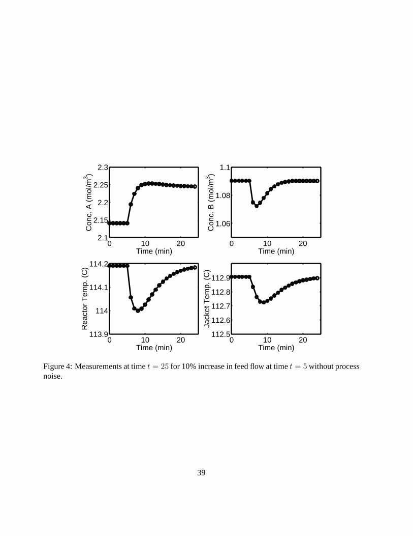
estimation method very accurately estimates the parameter value. For a representative example,
see the measurements in Figure 4. These measurements are taken from the reactor model after a
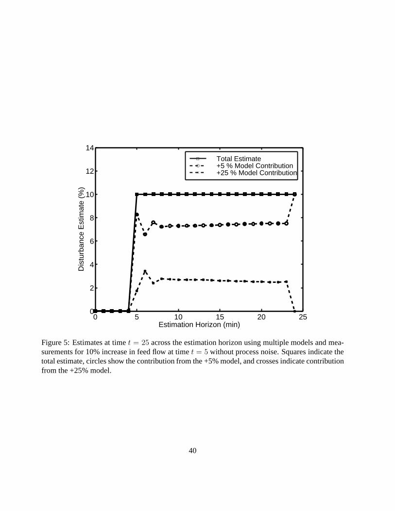
10% increase in the feed flow rate at timet = 5 minutes. Figure 5 shows the results for estimating
this 10% increase in the feed flow at timet = 25. The 10% increase affects the system 20 minutes
before this estimation result was computed. The two models used to estimate the total parameter
are shown. As one can see in Figure 5, both the 5% model and the 25% model are used when
estimating a 10% disturbance. The two model estimates can be summed directly because the mod-
els were normalized before the optimization took place. In Figure 6, the same fault measurements
are shown, but normally distributed noise (σ2 = 0.01) is now added to the signals. The resulting
estimates are shown in Figure 7. The accuracy of the resulting estimates degrades with the addition
of significant noise, but the correct fault is detected. In Figure 8, the estimation results using single
models for estimation are shown. As can be seen, the estimates are not as accurate as the multi-
ple model noise-free case, with slight deviation occurring across the horizon. The correct fault is
distinguished from the others, but the estimates are slightly in error when not using the multiple
linear models.
The evolution of a fault over time is also of interest. This estimation method estimates the
value of the parameters over the entire horizon, not just the current estimate or the initial value
23

estimate. In Figure 9, the actual input values over the estimation horizon for different times are
shown. At each sampling time, new measurements are available and the estimation process is
accomplished again. In Figure 10, the estimates over the moving horizon for different times are
displayed. After the fault is fully evolved, the amount of error in the estimate becomes larger. At
this point, the change in the measurements is becoming negligible, so any model error can lead to
increased estimation error.
In some cases, disturbances may affect a system as a ramp rather than a step. Figures 11 and
12 show measurements and estimates at timet = 25 for a gradual increase in the feed flow rate
starting at timet = 5 and slowly ramping up to +10% at timet = 25. The correct fault and
accurate level are detected.
This estimation method works well in multiple fault scenarios as well. In the following exam-
ple, the input feed flow rate is decreased by 20% at timek− 25 (t = 0) and the feed concentration
is decreased by 10% at timek − 15 (t = 10). The output measurements for this parameter change
are given in Figure 13. The overall parameter estimates for time k (t = 25) are shown in Figure
14. Here, the parameter estimates accurately picked the correct faults from the group of 20 and
also accurately estimated the parameter values.
Degenerate solutions may be possible in this system. Considering all the sets of faults con-
sisting of a single disturbance, the detectability analysis reveals that at least four other disturbance
responses must be used to represent a single fault. For systems with multiple faults, the analysis
could be used as needed to determine if degenerate solutions exist. Unique solutions should exist
for this example forS taking values 1 or 2.
24
4 Conclusions
In this paper, we have described a moving horizon method for detecting and estimating parameter
changes. The receding horizon formulation allows the use of a finite amount of data in the opti-
mization problem. This method makes use of multiple linear models to capture the behavior of the
actual nonlinear system. The problem is formulated as a MILP with an integer constraint on the
total number of changing parameters over the horizon.
There are limitations to this method, some of which have been described in this article. The use
of multiple linear models can lead to biased estimates in some cases. This will not always occur,
but can be seen in some mathematical examples. The results from one problem produce a potential
fault set. This set may not be the only set of faults that can accurately portray the existing data if
degenerate fault sets are available. This means that multiple causes may exist. Due to optimization
weights and a single optimal solution, it should be rare but possible to find different sets of faults
yielding the same or similar horizon based estimation results. Computationally, solving a large
scale MILP can be difficult. For multiple fault cases, enumerating all possible cases is typically
a poor solution. An improved MILP solution method is proposed that can exploit the problem
structure and existing information.
In the future, larger problems may be explored. In the proposed method, separate models for
positive and negative parameter shifts as well as small and large parameter shifts were used. Use of
linear models can allow for the solution of larger scale problems, but the system estimates should
be less accurate for nonlinear systems. This may be a reasonable tradeoff in systems where only
linear models are available and the process exhibits weak nonlinear character.
25

Acknowledgments
The authors would like to acknowledge financial support from the Office of Naval Research (grant
NOOO-14-96-1-0695) and the University of Delaware. The comments of anonymous reviewers
are also gratefully acknowledged.
Appendix: Nomenclature
a generalized optimization problem constraint matrix
Ar heat exchange area
b generalized optimization problem vector
B arbitrary positive value
c generalized optimization problem objective coefficients
CA concentration of speciesA in the reactor
CAO concentration of speciesA entering the reactor
CB concentration of speciesB in the reactor
Cp heat capacity of the reaction mixture
CPK heat capacity of the coolant
D total number of faults in a degenerate solution
∆Θ variable representing the value ofΘ(i)−Θ(i− 1)
∆y variable representing value ofy − y
∆HRi heat of reaction for reactioni
Ei activation energy for reactioni
26

f variable for the integer values representing separate faults
fj single fault for faultj
fD set of faults that can produce identical process response
F total number of faults
FK flow rate of coolant into the jacket
H horizon length
i index for time
j index for faults
J value of the objective function
ki reaction rate coefficient for reactioni
kio Arrhenius pre-exponential factor for reactioni
k current time
kw heat exchange coefficient
LP Linear Programming problem
mK mass of coolant in jacket
M combined impulse response matrix
Mj impulse response matrix for a faultj
Mo,j,n impulse response matrix relating outputo to fault j using modeln
MP matrix formed for the propositional logic constraint
MQ vector formed according to values ofQ, the error weight on|∆y|
MR vector formed according to values ofR, the error weight on|∆Θ|
MΘ matrix formed for the∆Θ constraint
MILP a Mixed Integer Linear Programming problem
27

n index for models for a faultj
nj total number of models for a fault
no total number of process outputs
N number of faults in the subset used for find a set of equivalent faults
o index for the outputs
P large value
Q weighting matrix for∆y
Qk jacket energy transfer from reactor
QP Quadratic Programming problem
R weighting matrix for∆Θ
ρ density of reactor contents
s variable used to in the degenerate fault set formulation, limited to be greater than 0
S total number of faults allowed to occur over a horizon
t time
Θ total estimated parameter variable, limited to be greater than 0
Θj(i) total estimated parameter value for faultj at timei, limited to be greater than 0
θj,n(i) individual model parameter value for faultj, modeln, at timei, limited to be greater than 0
U arbitrary upper bound
υ temperature of the reactor
υK temperature in the cooling jacket
υko temperature of coolant entering the jacket
V volumetric flow rate of feedstock into the reactor
VR volume of the reactor
28

xc continuous variables in the optimization problem taking values greater than 0
xi integer variables in the optimization problem taking value 0 or 1
y(i) process measurement residual vector at timei
yo(i) process measurement value for outputo at timei
y(i) process model vector at timei
yo(i) process model value for outputo at timei
z variable used in the degenerate fault set formulation, limited to be greater than 0
References
[1] P. B. Balle, D. Fussel, and O. Hecker. Detection and Isolation of Sensor Faults on Nonlinear
Processes Based on Local Linear Models. InProc. American Control Conf., pages 468–472,
Albuquerque, NM, 1997.
[2] P. B. Balle, D. Juricic, A. Rakar, and S. Ernst. Identification of Nonlinear Processes and
Model Based Fault Isolation Using Local Linear Models. InProc. American Control Conf.,
pages 47–51, Albuquerque, NM, 1997.
[3] A. B. Banerjee, Y. Arkun, B. Ogunnaike, and R. Pearson. Estimation of Nonlinear Systems
Using Linear Multiple Models.AIChE J., 43(5):1204–1226, 1997.
[4] A. Bemporad, D. Mignone, and M. Morari. Moving Horizon Estimation for Hybrid Systems
and Fault Detection. InProc. American Control Conf., pages 2471–2475, San Diego, CA,
1999.
29

[5] C. Chang and J. Chen. Implementation Issues Concerning the EKF-based Fault Diagnosis
Techniques.Chem. Eng. Sci., 50(18):2861–2882, 1995.
[6] C. Chang, K. Mah, and C. Tsai. A Simple Design Strategy for Fault Monitoring Systems.
AIChE J., 39(7):1146–1163, 1993.
[7] H. Chen, A. Kremling, and F. Allgöwer. Nonlinear Predictive Control of a Benchmark CSTR.
In Proc. of the European Control Conf., pages 3247–3252, Rome, Italy, 1995.
[8] L. W. Chen and M. Modarres. Hierarchical Decision Process for Fault Administration.Com-
put. Chem. Eng., 16(5):425–448, 1992.
[9] R. Dunia and J. Qin. Subspace Approach to Multidimensional Fault Identification and Re-
construction.AIChE J., 44(8):1813–1831, 1998.
[10] R. Dunia, S. J. Qin, T. F. Edgar, and T. J. McAvoy. Identification of Faulty Sensors Using
Principal Component Anaylsis.AIChE J., 42(10), 1996.
[11] S. Engell and K.-U. Klatt. Nonlinear Control of a Non-Minimum-Phase CSTR. InProc.
American Control Conf., pages 2941–2945, San Francisco, CA, 1993.
[12] J. M. Flaus and L. Boillereaux. Moving Horizon State Estimation for a Bioprocess Modelled
by a Neural Network.Trans. Inst. Meas. Control, 19(5):263–270, 1997.
[13] B. A. Foss, T. A. Johansen, and A. V. Sorensen. Nonlinear Predictive Control Using Local
Models - Applied to a Batch Process. InIFAC Symposium on Advanced Control of Chemical
Processes, pages 225–230, Kyoto, Japan, 1994.
30

[14] P. M. Frank and N. Kiupel. FDI with Computer-Assisted Human Intelligence. InProc.
American Control Conf., pages 913–917, Albuquerque, NM, 1997.
[15] M. Iri, K. Aoki, E. O’Shima, and H. Matsyama. An Algorithm for Diagnosis of System
Failures in the Chemical Process.Comput. Chem. Eng., 3:489–493, 1979.
[16] T. A. Johansen and B. A. Foss. Constructing NARMAX Models Using ARMAX Models.
Int. J. Control, 58(5):1125–1153, 1993.
[17] S. McGinnity and G. Irwin. Nonlinear State Estimation Using Fuzzy Local Linear Models.
Int. J. of Systems Science, 28(7):643–656, 1997.
[18] D. Mignone, A. Bemporad, and M. Morari. A Framework for Control, Fault Detection, State
Estimation, and Verification of Hybrid Systems. InProc. American Control Conf., pages
134–138, San Diego, CA, 1999.
[19] R. Murray-Smith and T. A. Johansen, editors.Multiple Model Approaches to Modelling and
Control. Taylor and Francis, London, 1997.
[20] K.R. Muske and T.F. Edgar.Nonlinear Process Control, M. Henson and D. Seborg, chapter
6. Nonlinear State Estimation, pages 311–370. Prentice Hall, 1997.
[21] D. S. Nam, C. Han, C. Jeong, and E. S. Yoon. Automatic Construction of Extended Symptom-
Fault Associations from the Signed Digraph.Comput. Chem. Eng., 20:5605–5610, 1996.
[22] T. Ohtsuka and H. A. Fujii. Nonlinear Receding-Horizon State Estimation by Real-Time
Optimization Technique.Journal of Guidance, Control, and Dynamics, 19(4):863–870, 1996.
31
[23] C.V. Rao and J. Rawlings. Nonlinear Moving Horizon State Estimation. InInternational Sym-
posium on Nonlinear Model Predictive Control: Assessment and Future Directions, pages
146–163, Ascona, Switzerland, 1998.
[24] D. Robertson and J. H. Lee. Integrated State Estimation, Fault Detection, and Diagnosis for
Nonlinear Systems. InProc. American Control Conf., pages 389–392, San Francisco, CA,
1993.
[25] A. Rueda. Approximation of Nonlinear Systems by Dynamic Selection of Linear Models.
In IEEE Canadian Conference on Electrical and Computer Engineering, pages 270–273,
Waterloo, Canada, 1996.
[26] L. P. Russo and R. E. Young. Moving-Horizon State Estimation Applied to an Industrial
Polymerization Process. InProc. American Control Conf., pages 1129–1133, San Diego,
CA, 1999.
[27] H. Tong and C. M. Crowe. Detecting Persistent Gross Errors by Sequential Analysis of
Principal Components.AIChE J., 43(5):1242–1249, 1997.
[28] M. L. Tyler and M. Morari. Qualitative Modeling Using Propositional Logic. InAIChE Fall
National Meeting, Chicago, 1996.
[29] M. L. Tyler and M. Morari. Propositional Logic in Control and Monitoring Problems.Auto-
matica, 35:565–582, 1999.
[30] K. Watanabe and D. M. Himmelblau. Incipient Fault Diagnosis of Nonlinear Processes with
Multiple Causes of Faults.Chem. Eng. Sci., 39(3):491–508, 1984.
32

[31] E. Yaz and N. Yildizbayrak. Moving Horizon control and Moving Window Estimation
Schemes For Discrete Time-varying Systems.Int. J. Sys. Sci., 18(8):1447–1456, 1987.
[32] K. Yin. Minmax Methods for Fault Isolation in the Directional Residual Approach.IFAC
Symposium, On-Line Fault Detection and Supervision in the Process Industies, 1992.
[33] Q. Zhang, M. Basseville, and A. Benveniste. Fault Detection and Isolation in Nonlinear Dy-
namic Systems: A Combined Input-Output and Local Approach.Automatica, 34(11):1359–
1373, 1998.
33

Figure Captions
Figure 1: Modified branch and bound example for dual fault case with 20 possible faults. Node
numbers indicate solution order and node sizes represent the size of the corresponding LP relax-
ation.
Figure 2: Steady state locus for simple example,dxdt
= −x − (d − 1)2, xo = −1, y = x + 1,
showing input multiplicity.
Figure 3: Response of CSTR model to step changes in the feed flow rate at time 0, with the
initial steady state feed flow = 14.9. Input multiplicity and both minimum and nonminimum phase
behavior are apparent.
Figure 4: Measurements at timet = 25 for 10% increase in feed flow at timet = 5 without
process noise.
Figure 5: Estimates at timet = 25 across the estimation horizon using multiple models and
measurements for 10% increase in feed flow at timet = 5 without process noise. Squares indi-
cate the total estimate, circles show the contribution from the +5% model, and crosses indicate
contribution from the +25% model.
Figure 6: Measurements at timet = 25 for 10% increase in feed flow at timet = 5 with
normally distributed noise (σ2 = 0.01).
Figure 7: Estimates at timet = 25 across the estimation horizon using multiple models and
measurements for 10% increase in feed flow at timet = 5 with normally distributed noise (σ2 =
0.01). Squares indicate the total estimate, circles show the contribution from the +5% model, and
crosses indicate contribution from the +25% model.
Figure 8: Separate estimates at timet = 25 using measurements from a 10% increase in feed
34

flow at timet = 5 using single models in both cases.
Figure 9: Actual parameter values over estimation horizon for 10% increase in feed flow at
time t = 5.
Figure 10: Horizon parameter estimates for 10% increase in feed flow at timet = 5 using
multiple models with constraint allowing a single fault across estimation horizon.
Figure 11: Measurements at timet = 25 for ramped change in in feed flow rate to +10% at
time t = 25 starting at timet = 5 without process noise.
Figure 12: Estimates at timet = 25 using measurements for ramped change in in feed flow
rate to +10% at timet = 25 starting at timet = 5 without process noise.
Figure 13: Measurements for dual fault case at timet = 25 with -20% input feed flow step at
time t = 0 and -10% feed concentration step at timet− 15.
Figure 14: Estimates at timet = 25 using measurements for dual fault case with -20% input
feed flow step at timet = 0 and -10% feed concentration step at timet− 15.
Table 1: Output response for example problem. ModelsM1 andM2 are developed from chang-
ing d from a value of 0 to values of1 and1.8, respectively.
Table 2: Van der Vusse CSTR model parameters.
Table 3: Potential faults for CSTR case study.
35

21
X
2021 ...
X 40
X 5922 39
41 42 58
20 Possible faultsMaximum of 2 faults
...
...
Best objective: -2.22, f1+f6
Best objective: -1.04, f2+f5
f1=1 f1=0
f2=1 f2=0
Objective: -0.92
Objective: -3.4119 cases with f1=1
18 cases with f1=0, f2=1
Figure 1: Modified branch and bound example for dual fault case with 20 possible faults. Nodenumbers indicate solution order and node sizes represent the size of the corresponding LP relax-ation.
36

−10 −5 0 5 10−120
−100
−80
−60
−40
−20
0
20
Out
put l
evel
Input Level
Figure 2: Steady state locus for simple example,dxdt
= −x − (d − 1)2, xo = −1, y = x + 1,showing input multiplicity.
37

0
10
20
30
40
0
10
20
30
400
0.5
1
1.5
Feed Flow Rate (m3/h)Time (min)
Con
c. B
(m
ol/m
3 )
Figure 3: Response of CSTR model to step changes in the feed flow rate at time 0, with the initialsteady state feed flow =14.19 l
h. Input multiplicity and both minimum and nonminimum phase
behavior are apparent.
38
0 10 202.1
2.15
2.2
2.25
2.3
Time (min)
Con
c. A
(m
ol/m
3 )
0 10 20
1.06
1.08
1.1
Time (min)
Con
c. B
(m
ol/m
3 )
0 10 20113.9
114
114.1
114.2
Time (min)
Rea
ctor
Tem
p. (
C)
0 10 20112.5
112.6
112.7
112.8
112.9
Time (min)
Jack
et T
emp.
(C
)
Figure 4: Measurements at timet = 25 for 10% increase in feed flow at timet = 5 without processnoise.
39
0 5 10 15 20 250
2
4
6
8
10
12
14
Estimation Horizon (min)
Dis
turb
ance
Est
imat
e (%
)
Total Estimate+5 % Model Contribution+25 % Model Contribution
Figure 5: Estimates at timet = 25 across the estimation horizon using multiple models and mea-surements for 10% increase in feed flow at timet = 5 without process noise. Squares indicate thetotal estimate, circles show the contribution from the +5% model, and crosses indicate contributionfrom the +25% model.
40

0 10 202.1
2.15
2.2
2.25
2.3
Time (min)
Con
c. A
(m
ol/m
3 )
0 10 20
1.06
1.08
1.1
Time (min)
Con
c. B
(m
ol/m
3 )
0 10 20113.9
114
114.1
114.2
Time (min)
Rea
ctor
Tem
p. (
C)
0 10 20112.5
112.6
112.7
112.8
112.9
Time (min)
Jack
et T
emp.
(C
)
Figure 6: Measurements at timet = 25 for 10% increase in feed flow at timet = 5 with normallydistributed noise (σ2 = 0.01).
41

0 5 10 15 20 250
2
4
6
8
10
12
14
Estimation Horizon (min)
Dis
turb
ance
Est
imat
e (%
)
Total Estimate+5 % Model Contribution+25 % Model Contribution
Figure 7: Estimates at timet = 25 across the estimation horizon using multiple models andmeasurements for 10% increase in feed flow at timet = 5 with normally distributed noise (σ2 =0.01). Squares indicate the total estimate, circles show the contribution from the +5% model, andcrosses indicate contribution from the +25% model.
42

0 5 10 15 20 250
2
4
6
8
10
12
Est
imat
ed p
aram
eter
cha
nge,
(%
)
Estimation horizon (min)
+5 % Model
0 5 10 15 20 250
2
4
6
8
10
12
Est
imat
ed p
aram
eter
cha
nge,
(%
)
Estimation horizon (min)
+25 % Model
Figure 8: Separate estimates at timet = 25 using measurements from a 10% increase in feed flowat timet = 5 using single models in both cases.
43

t−20t−10
t 010
2030
4050
0
5
10
15
Time t (min)Feed Flow over horizon at time t
Act
ual f
eed
flow
cha
nge
(%)
Figure 9: Actual parameter values over estimation horizon for 10% increase in feed flow at timet = 5.
44

t−20t−10
t 010
2030
4050
0
5
10
15
Time t (min)Horizon estimate at time t
Est
imat
ed f
eed
flow
cha
nge
(%)
Figure 10: Horizon parameter estimates for 10% increase in feed flow at timet = 5 using multiplemodels with constraint allowing a single fault across estimation horizon.
45

0 10 202.1
2.15
2.2
2.25
2.3
Time (min)
Con
c. A
(m
ol/m
3 )
0 10 20
1.06
1.08
1.1
Time (min)
Con
c. B
(m
ol/m
3 )
0 10 20
113.6
113.8
114
114.2
114.4
Time (min)
Rea
ctor
Tem
p. (
C)
0 10 20112.5
112.6
112.7
112.8
112.9
Time (min)
Jack
et T
emp.
(C
)
Figure 11: Measurements at timet = 25 for ramped change in in feed flow rate to +10% at timet = 25 starting at timet = 5 without process noise.
46

0 5 10 15 20 250
2
4
6
8
10
12
14
Estimation Horizon (min)
Dis
turb
ance
Est
imat
e (%
)
Figure 12: Estimates at timet = 25 using measurements for ramped change in in feed flow rate to+10% at timet = 25 starting at timet = 5 without process noise.
47

0 10 202.1
2.2
2.3
2.4
Time (min)
Con
c. A
(m
ol/m
3 )
0 10 200.95
1
1.05
1.1
Time (min)
Con
c. B
(m
ol/m
3 )
0 10 20112
112.5
113
113.5
114
Time (min)
Rea
ctor
Tem
p. (
C)
0 10 20111
111.5
112
112.5
113
Time (min)
Jack
et T
emp.
(C
)
Figure 13: Measurements for dual fault case at timet = 25 with -20% input feed flow step at timet = 0 and -10% feed concentration step at timet− 15.
48

0 5 10 15 20 25
−20
−15
−10
−5
0
Est
imat
ed C
hang
e in
F
eed
Flo
w R
ate
(%)
0 5 10 15 20 25
−10
−5
0
Estimation Horizon (min)
Est
imat
ed C
hang
e in
Fee
d C
onc.
(%
)
Figure 14: Estimates at timet = 25 using measurements for dual fault case with -20% input feedflow step at timet = 0 and -10% feed concentration step at timet− 15.
49

t y (∆d = 1) y (∆d = 1.8) M1 M2 y (∆d = 1.7)0 0 0 0 0 01 0.63 0.23 0.63 0.13 0.322 0.86 0.31 0.23 0.05 0.443 0.95 0.34 0.09 0.02 0.484 0.98 0.35 0.03 0.01 0.505 0.99 0.36 0.01 0 0.516 1 0.36 0 0 0.51
Table 2: Output response for example problem. ModelsM1 andM2 are developed from changingd from a value of 0 to values of1 and1.8, respectively.
50

Table 3: Van der Vusse CSTR model parameters.k1o = 1.287 · 1012 h−1 k2o = 1.287 · 1012 h−1 k3o = 1.287 · 1012 m3
molAh−1
E1 = −9758.3K E2 = −9758.3K E3 = −8560K∆HRAB = 4.2 kJ
mol A∆HRBC = −11 kJ
mol B∆HRBD = −41.85 kJ
mol A
ρ = 0.9342 kgl
CP = 3.01 kJkgK
CPK = 2.0 kJkgK
kw = 4032 kJhm2 K
AR = 0.215m2 mk = 5.0 kg
VR = 10 l FKC = 10.52kgh
vko = 60C
V = 14.10 lh
51

Table 4: Potential faults for CSTR case study.
f1 increase in feed flow rate f2 decrease in feed flow ratef3 increase in coolant flow rate f4 decrease in coolant flow ratef5 increase in feed temperature f6 decrease in feed temperaturef7 increase in coolant temperature f8 decrease in coolant temperaturef9 increase in feed concentration f10 decrease in feed concentrationf11 increase in jacket heat transfer coefficientf12 decrease in jacket heat transfer coefficientf13 increase inCa measurement bias f14 decrease inCa measurement biasf15 increase inCb measurement bias f16 decrease inCb measurement biasf17 increase inυ measurement bias f18 decrease inυ measurement biasf19 increase inυk measurement bias f20 decrease inυk measurement bias
52