Annals q/Glaciology 25 1997 [ International Glaciological Society

Use of ice-sheet nortnal tnodes for initialization and tnodelling stnall changes

RICHARD C. A. HI;\IDMARSH,

British Antarctic Survq" Valllml Environment Research COllncil, High Cross. J ladillgl~J' Road, Cambridge CB3 OET, England

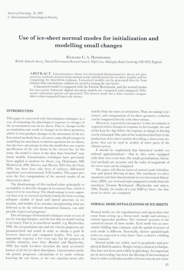
ABSTRACT. Linearizat ions abo ut t\\·o hor izon ta l-dimensiona l ice shee ts arc pro­posed as methods of generating normal mode initi a li zatiolls for ice-sheet models a nd for computing the short-term response. Linearized models ca n be gene ra ted directly from balance-nux calc ulati ons without the need fo r tuning the rate factor.

A linea ri zed model is compared with the Eismint Benchmark, and the normal modes [or two coarse Antarctic dig ita l elevation models a rc computed and compared. Volu­metric relaxat ion spec tra a rc presented. The slowest mode has a time constant compar­able to tha t computed [i'om sca le theory.

INTRODUCTION

This paper is conce rned with linearizati on techniques as a way of estimating the glaeiological response to changes in the accum ul ation rate on ice sheets. That is, cha nges in the acc umul at ion rate result in changes in ice-sheet geometry, which in tllrn producc changes in the movement of the ice. Linearizedmethods have, of coursc, some disad\·a lllages in modelling the non-linear eyolution eq uati ons for iCT sheet s, but a lso ha\"(' advantages in that the model does not require specificat ion of the rate factor in the viscous law. In thi s sense, the model is closer to the da ta th an "matched" non­linear models. Lineari za ti on techniques ha\·e prC\·iously been applied to modern ice sheets (e.g. Oerlemans, 1981; Hindm ars h, 1992; Drewr), a nd lVforris, 1992; Va n der \ 'een, 1993), but these ha\"C only been of ordina ry differential eq uations (zero-dimensional (O-D )models). This paper pre­sents the fi rst computa tions of the normal modes of an obsern'd ice sheet.

The disadyantages of thi s method rclate principa lly to an inability to describe changes in ice-stream flow, which is expectC'dto be non-linea r. The disad\'alllage is morC' appa l-­enr than real , as resea rch methods remain far from creating adequate models of basal and latera l processes in ice streams, a nd models of ice streams, incorporating what are beli e\"Cd to be the rele\'ant dynamical features, can only provide conjectura l prognoses.

The ack a ntages oflin earized techniques relate to ease of use for non-g laciologists, a nd the fact that no model tuning is necessary. That is, in non-linear models (e.g. Huybrechts, 1992) the acc umul ation rate and the viscous properties are parameterized a nd tuned in order to obtain a good fit between obsen ·ed and computed heights. This was an appropriatC' respo nse a few yea rs ago, but the progress of satellite a ltimetry since then (Bambe r a nd Huybrechts, 1996) has made ice-shee t e1 e\'a tion the most accu rate ly

known of a ll the icc-sheet descriptors. Linearization meth­ods permit prognostic calculations to be made without knowing the rate fac tor, as the rate eq uation stems ulti-

matel)' from the mass acc umulation. Thus, no tuning is ne­cessa ry a nd computat ions of ice-sheet geometry e\'o lution can be compa red directl y with observations.

1\ \oreO\"Cr, a practical consequence is that no estimate is required of slow cha nges in response to, for example, the end of the Last lee Age before the response to changes in forcing

can be estimated. Onc a i m of the work descr ibed here is the production of ice-shee t models describing a short-term res­ponse that can be used in model s of other pans of the clim a te sys tem.

it should be emphas ized that lineari zed models a rc rat iona l approx im ations - that is, they come equipped

with their own error bars. For small perturbations, linear­ized methods a re accurate a nd the order of magnitude of the error term ca n be computed.

The paper wi ll discuss issues of normal mode initi a liza­ti on a nd spatia l filter ing of data . The non-linea r ice-shee t equat ions and their Iinear izations in two horizontal dimen­sions (2HD), a rc IT\·iewed and compared to results from the non-linear Eism int Benchmark (Huybreehts and others, 1996). Finally, the modes of a rea l 2HD ice sheet (the An t­a rel ic ice sheet) arC' computed.

NORMAL MODE INITIALIZATIONS OF ICE SHEETS

Normal modes arc the eigenfunetions and eigen\"alucs th at C'nsue frOIll. sell ing up a linear (ized ) model and so lving a related eige lwa lue problem. The "normal'· pertains to the canon ical nature of thcse modes. Each mode has an asso­ciated e-folding time consta nt, and the spati a l structurc of each mode is different. Essentially, shoneI' sp ati al-leng th scales arc expee tcd to relax fas ter (ha\"C a shorter e-folding time consta nt ).

Normal modes a rc widely used in geophys ics and geo­physical nuid dynamics. D espite being a class ica l technique,

they haY(' not becn used widely in glaciology. An importa nt use in meteorology has been the filt ering of meteorological data in order to initi a li ze models with data that do not exc ite

85

Hindmarsh: Ice-sheet normal modes and modelling small changes

non-physical numerical modes. As explained above, ice-sheet-model geometr y, when

compared to real data, represents a trade-off be twee n the tuning of the rate fac to r and the parameteri zation of the accumulation-rate di stribution. An obvious iss uc is whcther norma l mode techniques can be exploited to initia li ze ice­sheet models. In pa rticula r, the adve nL of satellite altimetry has produced very acc urate cle\'ation data that necd to be included in ice-sheet models if dynamics a re to bc inferred from obscrvations.

When obsen 'ed elevations a re used in non-linear ice­shee t models, it is found that sma ll er-scale structure is re laxed out quickly, sometimes causing numerical problems (O erl emans and Van der Veen, 1984). C urrent observations of basal topography a re nowhere near the same pl a n-view resolution, meaning that er rors in the thickness cause com­puted a nd spurious ice-flow anoma lies, resulting in the nu­merical smoo thing de cribed above.

A n obvious question is whether normal-mode initi ali za­ti on techniques can be used in some fo rm in ice-sheet mod­elling, with the specific obj ec ti\Oe of ensuring that obsen 'a tions a rc used as an initi al sta te, rather tha n some trade-ofT between ignorance of acc umulation, rate factor,

ice-shee t thickness and the need to ma intain numeri ca l sta­bilit y.

Because the ice-shee t equati on represents a n initi a l value problem, any measured data a re physica ll y consistent. Anom alous roughness and topographic sinks (e.g. the

Vostok depression) could simply be rel axing out. U nder an ass umption of steady sta te, the orig in of many features becomes lTlOre problematica l, but can still , in principle, be expla ined by local \'a l' ia ti ons in the poorly known basal topography o r, in a more contri ved way, by local vari ations in the rate fac tors fo r interna l deformation or for sliding.

Topographic dcpressions can a ri se as a res ult of locally en­hanced basal melting, or may conceivably occur as a res ult of "S tokes effec ts", whel-e, fo r example, sma ll-scale vari a­tions in the basa l topography res ult in local failure of the shallow-ice approxima ti on (e.g. J 6hannesson, 1992).

Sma ll-sca lc (waveleng th of a few g ridcell s) surface

roughness, tha t is not refl ected in causatory vari a ti on in

thc rate factor or the basal topography, is relaxed out by the action of non-linear so lutions. Ba la nce-flux calcul ations a nd ensuing linea ri zati ons a rc not affec ted by this problem provided topographic depressions a rc dealt with by se tting basal melting to be la rger tha n the acc umulation.

Such noisy da ta can be dea lt with in several ways when initi a li zing models:

(a ) Accept the data as a valid zeroth-order approximation

and compute a se t of eigenful1ctions and eigenvalues. Tt

could transpire that even the low wave-number eigen­

fun ctions a re noisy.

(b) Smooth heuristicall y and compute the norm al modes.

(c) Select a smooth zeroth-order solution on a n error mini­mization criteri on and compute the norma l modes (Hind marsh, in press ).

In the latter two cases there will be a res idual between the zeroth-order solution a nd the da ta. This can be reduced by fittin g the res idua l with the normal modes: thi s is a nor­mal mode initialization as commonl y used in other geo­sciences (e.g. Da ley, 1992). The more modes used , the small er the waveleng th of feature tha t can be modelled.

86

The rema ining va ri ation is filtered by using fun cti ons that h ave a close rel a ti on to ice-sheet physics rather than by a n a rbi trary smoothi ng.

C learl y, if option (a ) produces smoo th norma l modes, then it is the simplest opti on. Prov ided sink-holes a re elimi­nated from the observed data, then the computed normal modes do not appear noisy. It is possible that holes could be reconstituted by using the normal modes, but testing the effi cacy of this technique is outside the immedi ate aims of thi s paper. We shall see tha t option (a ) is possible.

THE ICE-SHEET EQUATION AND ITS LINEARIZA­TIONS

Nota tion is summa ri zed in Table I. "Vhen considering the mecha nics of ice sheets a reduced model is norma ll y used (Hutter, 1983; M orl and, 1984; Fowl er, 1992), obtained from a

sca ling of the Stokes equations. The scaling yields sim ple fun cti ona l forms for the vertica l vari ati on of the stress field and a considerable computa tiona l sav ing. Further manipu­lati on of the reduced model results in the ice-sheet equation:

(1)

where H(x, y. t ) is the thickness of the ice shee t, s(x , y, t) is the upper surface a nd a is the surface mass-ba lance ex­change. Bou nda ry conditions for th is model a rc:

8tH (:c, V(x) , t) == 0 , (2)

where y = V (x) , the presc ribed margin. This co rres ponds

to the Vi a lov- Nye ca lving condition, where the ice thickness at the ma rgin is less than the max imum thickness. l\IIo re advanced models, to be considered in fUlUre work, would have non-ze ro thi ckness a t the g rounding line a nd a moving grounding line. This has a lready been treated in a linear­

ized fashion for one hori zonta l dimension (IHD) by Hind­marsh (l996a).

These evolution equations describe the evolution of ice­sheet thickness where the fl ow mecha ni sm is either i11lerna l deformation aecording to a non-linearly viscous fl ow law or

Table 1. No! ation

I (friable

a

C!­h

k e 7Il

q S

Slk : SI' t (:r:,y, z) C' E

E F G H C. T /.I

oX

r

J/eanin,t;

Accum ulati on rate

Spati a l modes Or Sk; Fo uri er tra nsform of T

Vector over e of H I Spati a l mode index Joi:llIri cr mode index Poi nt index Non-l inear diff usio n index Flux of ice Ice-shee t el c, oat ion

Fo uri er component for point [at frcqucncy k, 'Tctor ove r f Time

Space coordinates R ate factor Eigenfunctions of C. \ lat ri x o (" c ige l1\TC lOr S

Disc rcti zatio l1 o f £:,

Discrct ized G reen's fi.lllc ti on co rresponding to c. - I l ee-shee t thi ckness

Linea r-pertu rbat ion opera tor Vector of mode a mplitudes Flow/slid ing-law index Eigenva llles ~I at ri x ofcigeJ1 \'al ucs

sliding according to a \Veertma n-type law. The a na lyses ca r­ried o ut in thi s paper arc not limited to these situa tions.

The qua ntit y C is directl y rel a ted to eith er a weightcd ITrtical aycrage ra tc fac tor Ad defin ed below in Equa ti on (6) of the rate facto r Ad Llsed in thc I' iscous rela tionship:

(3)

where E is a second im'a ria nt of the deformation ra te a nd T

is a second im'a ri a nt of the devia tor stress (G len, 1955) o r comes from a slidi ng rela ti on of the form :

(4)

(\\'ee rtma n, 1957). We construct the foll owing qua ntities fo r

use in the genera l el'o lution equati on:

7n= {'II + 2 (+ 1

{Internal deformat ion Sliding.

The deril'a ti on of the el 'olution Equati on (1) using the sha llow-ice approx im ation is sta nda rd (Hutter, 1983; 1\101'­la nd, 1984: Fmvler, 1992), A furth er standa rd der il'a ti on, which, in the present nota ti on, ca n be (o und in Hindmal'sh

(1996a) yields a formul a fo r the ice Oux q:

. - -CH illi " 1

,

/-1", ql - v S u .r;S (5)

where:

(6)

Irinstead we a rc dea ling w ith sliding, then:

(7)

a nd use of the continuit y equati on:

(8)

result s in the non-linea r diffusion type Equati on (I). Linear­izati ons a rc computed by ex pa nding H a nd a in a . cri es

H = Ho + pB\ + . , , , a = ao + J.W ] + ....

a nd trunca ting a t first order. The'L'1ylor expa nsion ofq.r, fo r exa mple, yields:

Spec ifica lly, we can compute:

Oqil H III- ]I" I,,-t;::. IH oH = 7H 0 v So u .r, sQ = -rnqiil 0 HI!

Hindmarsh: Ice-sheet norllla! modes and //lode/ling small changes

a nd we can sce that the zeroth order a nd (i rst-o rder equa­ti ons a rc:

'\l . qo =ao - a/ H o

a/ H I = - '\l , q j +al.

{m H I

qi] = f] iO --+ H o

(9)

(10)

0,,5] }.

(ll )

Bo unda ry conditi ons a rc the crude approx im ation of fi x ing the eleva ti on a t the ma rg in o f the ice shee t. 1\[m' ing bo und­a ri es can be inco rporatcd into linea rizatio ns (Hindma rsh,

1996a ) but the technica l difficulti es of' ex tending this approach to two horizonta l dimensions mean that it is 1,I'o rth il1lTstigating the fi xed ma rg in problem li rs t in o rder to as­sess the potenti a l oflinea ri zati on techniques. Abl ating m a r­g ins are not considered in thi s pa per.

The zeroth- order so lution ca n be identifi ed Irith the

long-term trend (c.g. the res ponse to p re-industri a l climate conditions) a nd the first-order solution with the fas ter res­ponse to perturbatio n. The long-term trend co uld of course be stead y sta te. If the technique were being applied rigo r­ously time should be expanded in tlYO timc-scales, but the

complexiti es o f the required nota tion outweig h the benefit s,

so the procedure is justili ed heuri sticall y by saying that the pe rturbation is expec ted to grow over time-scales where the zeroth- order so lutio n ha rdl y cha nges, a nd a "snap-shot" ca n be ta ken 0 [' the pro til e to compute the coe lli cients in Equa­ti on (9)

The curio us way of writing the zeroth-order equati on is

to emphasize tha t ignora nce of acc umulati on rate a nd ra te o r cha nge or surface profi le have exac tly the same sig nifi­cance. It is ass umed that al is kn own, in the sense that the response to a postul a ted cha nge in the acc umul ati on ra te is being cva lua tcd .

i\ sig nifica nt feature of the perturbati on equati on is the absence of the ra te factor in the first-order equation, Th e time dimension is introduced into the ice-shee t equati on by the acc ulllul a ti on ra te of snow a nd th ro ug h the ra te fac tor. In a stra in-ra te cont rolled no\\', such as is ass umed here, the ice sheet ex ists to di scha rge the snOl\'fall , a nd the time-sca les a rc se t by meteo rologica l factors. The ice-shee t geo metry

adjusts so as to set the rh eo logica l time-sca le equa l to the meteorol og ica l time-sca le. \Vhere there a rc intern al osc ill a­tions in the icc shcet, the fas t a nd 5101\' phases correspond to

stress-controll ed no\\'s, a nd the perturbati on equa ti on will not appl y. In a ny case, the perturbatio n equati on is a linea r equa tion a nd ca nnot halT limit cyele soluti ons such as those

desc ribed by Pay ne (1995). By se tting ClI = 0 the linea r equati on can be pu t into

homogeneous form. A sepa ra tion of I'a ri ables technique can be used to ge nerate so lutions to the homogeneous fo rm using an eige nl'a lue expansion, which can subsequentl y be used to construct solutions to the inhomogeneous fo rm .

The theory is IT\'iell'ed below. In genera l, the eigenprobl em

has to be sohTd numerica ll y, Thcre a re potenti a l problems associated with sing ul a r behm' iour a t the divide a nd ma rgin.

Hindma rsh (l996b, in press ) has conside red perturba­ti ons abo ut the IHD Via lOl ' Nyc (Vl'\ ) (Vi a lm', 1958; Nye, 1959) solution, Il' hich is computed by se tting o,H = 0 a nd

a = allIO. C = C,lia, both consta nts, into the pla ne-Oow I'er­sion of Equation (I) a nd integrating the res ulting ordina ry differenti a l equation (ODE ). Hindm a rsh (in press ) trea ted

87

Hindl7larsh: Ice-sheet norma! modes and modeLLing small changes

the singula riti es at margin and divide acc urately by using Frobenius expansions (sce a lso Fowler, 1992). In the 2HD calculations reported here, Taylor expansions a rc used at the margin a nd at the di vide. Calculations fo r lHD, based on the principles desc ribed below for 2HD, show that this ma ke very littl e difference to the computed eigcn\'a lues or eigenfunctions. This presumably a rises as a result of the ro­bustness of Sturm- Liouville systems to model perturbation (Pryce, 1993). Taylor, rather than frobenius, expansions are a lmost universa lly used in ice-sheet modelling when the non-linear problem is treated.

ZEROTH-ORDER FLUX COMPUTATION CONSIS­TENT WITH FINITE-DIFFERENCE GRIDS

Given that the perturbation procedure will be carri ed out on a finite-difference g rid, it is highl y desirable that the zer­oth-order fluxes sati sfy the conservation equa tion exactly. For thi s reason, efficient shooting procedu res (Budd and vVarner, 1996; Rcmy and others, 199G) are not used. The pro­cedure is simply to compute the flux a rriving a t a g ridpoint from x- a nd y-direction conncctions, compute thc nux out

using continuity, and divide it between all the outlet connec­tion (i. e. to poi nts at a lower elevation ) in I i nea r proportion to their slopes.

Consider the coeffi cient D = CHb"IV sol,,- l. Then, q = - DVso. Even though So and Ho arc known, C is not, meaning that D is a lso unknown. A finite-differcnce approximation is:

_ D 8;+ l. j - S i.j Qi+ l / 2.j -; A

U J .

for each of the outlet points, where D; is an unknown. The

outlet discharges and D can be solved with the additional cquation:

q.i+ I/ 2.j - q.i- I/ 2.j + q i.j+ I/ 2 - q i.j- I/ 2 _ - a ij · 6 r 6 y .

Balancc nux calculations have bccn used by Remy a nd others (1996) to solve for thc rate fac tor and thcnce thc basal temperature.

In practice, the g rid-centred flu xes arc computed by sol­ving a set of linear equations. These satisfy continuit y ex­ac tly and also return the quantity D = CHo"II 'V sol'J- l. While the method is a lgorithmica lly different from tha t of Budd and' Varner (1996), the two methods eem to be consis­tent a t 0 (6 ., ) . The purpose of using a different method is to ensure that the continuity equati on is respected exactly at zeroth order on the finite-difference grid used to solve the eigenproblem.

THE EIGENVALUE PROBLEM AND ITS DISCRETI­ZATION

The first-order perturbation Equations (10) and (11) are conveniently written in operator form:

(12)

HI (x. y , t ) is written in a separablc form:

Hl (x, y, t ) = T (t )R (x, y)

88

a nd substitution of thi s into the homogeneous form ofEqu a­tion (12) yields:

T(t ) = .cR(.r;, y) = A T (t) R(.r; , y)

where A is an eigen\'a lue. The spa tial equation is:

.cR(x, y) - AR(x . y) = O. (13)

which has eigenvalue solutions £ (:c, y) . Now, in genera l it cannot be ass umed that the eigenfunc­

ti ons arc orthogona l, a nd it is a lso convenient simply to con­

sider eigenfunction expansions truncated after AI term s, a nd to consider the eigenfunctions evaluated a t AI points: this is what emerges from. solving the algebraic eigenva lue problem resulting ("rom the di sc reti za ti on of the operator .c. which is denoted by the matrix F. Suppose tha t R (:c, y) is represented by AI points sampled on the grid ; these points have value ri, e = (1. AI). Then, the matrix representa tion 0 [" Equation (13) is:

Fr - Ar = 0

where the di agona l entries of the matri x A are the eigenva­lues. This is an a lgebraic eigenvalue probl em (Wilkinson,

1965), which is sati sfi ed by AI linearl y independent eigen­vec tors. "Vc construct a matrix E the ith column of which is the i th cigenvec tor eva lua ted at !I f points. Thus, i is a n index of spatia l mode number.

It will be ass umed that these eigenfunctions a re linearl y independent and fo rm a complete se t - there have been no

cases found where this is not true. It may thus be written that:

= 00

Hl = LTi(t)E;(x , y), U I = L T;( t )a,(x. y)

a nd, after using Equation (13) the perturbation Equation (12) becomes:

L T; £ ; = L ,\;T;£ i+a, (x , y) E [-1, If. (l-J)

By sampling Equation (14) at !I f points, this equation may be written as a disc reti zed matri x equation:

ET = EAT + a (15)

where a is the vec tororaccumul ation rate sampled at the !I f points. There a re thus !If linea r equa ti ons corresponding to the !If points of evaluation, a nd the elevations a t the sampling points a rc given by:

h = ET.

where h is the vector of H u at the sampling points. By mul­tiplying Equation (15) by E - 1

. the existence of which is as­sured by the fact that the eigenvec tors a re independent, !I f mode-evolution equations a rc obtained:

(16)

with the TOWS of the im·erse eigenvector matri x pl aying the role or a modal we ighting runction in space for the acc umu­lation rate. By definiti on F = EAE- I

.

At steady state, we have EAT = - a , whence

(17)

where G = _ F - 1 plays a role a nalogous to a Green's func­ti on. A rcfinemelll is to suppose that N modes ha\'e suffi­ciently slow relaxation (sma ll eigenvalues ) tha t it is necessa ry to consider their dynamic va lues, ,,·hile the

rcm a llllllg L = j\1 - N m odes a rc regarded as being in steady state. Then, a qua ntit ), hL ca n be constructed which represents that pa rt of the perturbation th at relaxes suOI­cientl y quickl y to be in equilibrium II'ith the insta nt a neous

forcing. These a rc the so-ca ll ed "s lal"Cd" m odes, which a rc computed according to:

h L = G La,

G = E ' , A - 1 E - I L .. (:\ + lPI f \~I I' '' ,I\+IP I (:\ + 1 ):~ I. :

(l Sa)

(l Sb)

where colon (" ~1atlab" ) nota ti on is used in the subsc ripts

(Golub a nd Va n Loa n, 1989, p. 7). For example, the range of indices being considered a rc represented by a : b. with a single colon by eOIl\'C ntion IT jJl'esenting the to ta l ra nge.

H ere, G L can be rega rded as the G reen's ['uncti o n for the slaved m odes. The evolutio n of the rema i ning N d yna m ic modes is gil 'en by

(19)

so th at:

In practice, onc often does not w'ish to compute the whole

eige nl'a lue sequence, a nd it is a stra ightforwa rd exercise to show tha t:

G L = G - E I 'X A - 1 El~~ " ".. 1\ I \ . . ' ..

(20)

Thus, it is necessary to compute G, the ma tri x il1\ 'erse of the

operator matrix F , a nd those eigenvalues that rel ax su!Ti­

cientl y slowl y that wc a re imerested in their d ynamics. Trun­ca ti o ns of such genera li sed Fo uri er expansions of ice sheets ha\'C been considered by Hindma rsh (1990), who concluded that computa ti on of the evolution of a few dyna mic modes represented the el'o lution of the ice sheet reasonably well.

In IHD the first-order perturbati on Eq uations (10) a nd (11 ) can be written in Sturm- Lio uville form a nd soh-cd using either finite-difference methods or shooting methods

1.5

g I 'iij > ~ 05

(a) Eisbench elevation

......

o JjJ Ifllf Iflf IIf If If IfItHI,

" o

1

-0.1

';; -005 ;; ,

tii

o 1

y-PosiLion -I -I x-Position

(c) Forcing: in-phase component

..... .....

y-Position

.. . . : ..

-I -I x-Position

" .S?

HindJll G1:,h: Ice-sheet normal modes and modelling small changes

(Hindm a rsh, in press ). The eige nfunctions a rc orthogonal. In 2HD, this is not true in ge nera l a nd the perturba ti on eq ua t ion, \\'hich i ncl udes cross-dcrivativc terms, is d isc re­

tizcd using a sta nda rd nine-point consen 'a til'e stencil,

which produces a spa rse, non-symmetric matri x. The eigen­I'a lue problem \\'as so li-cd using the ARPACK softwa re (Sorensen, 1992) which dca ls spec ifIca ll y with la rge, spa rse, non-symmetric probl ems. The softwa re uses Arnoldi itera­ti on (sce e.g. Ch atelin , 1993), producing the "Ritz I'a lues·'.

II'h ich a re approx i mations to the eigell\'a l ues.

TEST: PERTURBATION TO THE EISMINT BENCH­MARK

The Eismim Benchma rks (EBs) (Huybrechts a nd others.

1996) arc a se t of benchma rk experiments desig ned for the purpose of model el'alua ti on. The isotherm a l VN bench­m a rk , \\'h ere unifo rm acc umul a ti on is presc ribed 0 11 a square domain \\,ithY)J ma rgins (i. e. ze ro thickness a nd fi­nite flu x of'i ce ) a rc not co nsidered here. It \\'ill be considered in the sca led doma in (.1', y) E [-1.1] X [-1.1] \\'ith unit

acc umul ation and ra te factor C. In thi s case, the zeroth

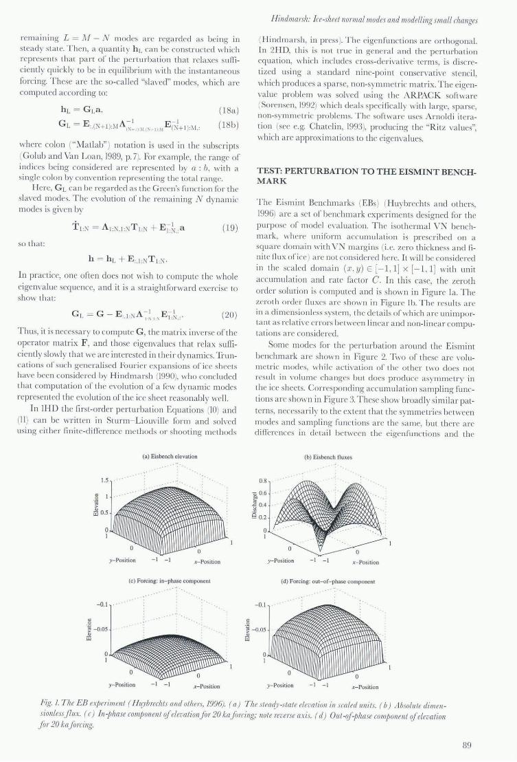
order so luti on is computed a nd is sho\\'n in Fig ure la. The zero th o rder (luxes a rc shown in Figure lb. The res ults a rc in a dimensio nless s>'s tcm, the deta il s oJ'\\'hich a rc unimpor­ta nt as rcl a ti\ 'C errors bet\\'een linear a nd non-linea r compu­ta ti ons a rc considered.

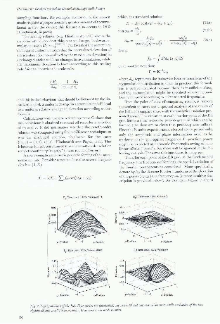
Some modes for the perturbati on aro und the Eismint benchm a rk a rc shown in Figure 2. T\\·o of thesc a rc vo lu­metric modes, while ac til 'a ti on of the other t\\'o does not result in \'o lumc cha nges but docs p roducc asy mmetr y in the ice shec ts. Corresponding acc umul ati on sampling fun c­

ti ons arc shOlI'Jl in Fig ure 3. These show broadl y similar pat­

terns, necessa ril y to the extent that the symmetri es between modes a nd sa mpling fun cti o ns a re thc same, but therc a re differences in deta il between the eigenfuncti o ns a nd the

O.S

" 0,6 ~ "§ 0.4

Q 0.2

o I

-0.1

(b) Eisbench fluxe s

y-Posilion -I -I x-Position

(d) Forcing: out-of-phase componenl

~ - 0,05

" tii

o lJIIIIIIIIIIIIIIIIIIII1111TtHi I

y-Posilion -I -I x-Position

Fig. I. Th e EB experiment (HI~yb /ec!tts al/ d ot/zers, 1996). (a) Th e steady-stale elfl'alioll in scaled IIl1ils. ( b) Absolute dimen ­sion!essjlu¥. (c) IIZ-jJ/zase componenl q[elevatiolZJor 20 kalo /cing; nole 1'aNSe alis. ( d) OUI-q[-phase component q[elevalion Jor 20 kafomllg.

89

H indmarsh: Ice-sheet normaL modes and modelLing smaLl changes

sampling functions. For example, activation of the slowes t mode requires a proportionately g reater a mount of acc umu­lation nearer the centre; thi s feature a lso occurs in IHD (H indm a rsh, in press).

The scaling rela ti on (e.g. Hindma rsh, 1990) shows the response of the ice-sheet thickness to cha no'es in the acc u-

I · . H 1!(7lI+v) b mu atlO n rate IS 0 ~ ao . The fac t that the acc umul a-tion rate is uniform impli es that the normali zed elevation of the ice-sheet (i.e. normalized by the maximum elevation) is unchanged under uniform changes in acc umula ti on, while the max imum elevation behaves according to thi s sca ling rul e. ' Ve can linearizc the scale r ul e:

dHo 1 Ho clao m + v ao

and this is the behav iour that should be followed by the lin­ear ized model: a uniform change in accumulation will lead to a uniform relati\ 'C change in elevation according to this formula.

Calcul ations with the di screti zed operator G show that thi s behm'iour is obtained to round ofT error for a selection of m a nd v. It did not matter whether the zeroth-order

solution was computed using finite-difference techniques or

was an ana lytica l solu tion, obta inable for the cases (m, v) = (0, 1), (3, 1) (Hindm arsh a nd Payne, 1996). This is because it has becn cnsured tha t the zero th-order solution respects continuity "exactly" (i. e. to round ofT error).

A more complicated case is period ic forc i ng of t he acc u­mulation rate. Consider a system forced at severa l frequen­cies k = (1. K )

t = AiTi + L h COS(Wkt + X.)

0.06

g 0.04 .'" '" > @O.oz

El ; Time const. 1142.; Volume 0.1 2

.' ....

? J.IIJ.,IllIlIlIlIlIlIrtf:

0.15

" 0.1

.S! ~ 0.05 " tU o

-0.05 I

y-Position -1 -I x-Posilion

E6

; Time const. 452,; Volume 0.055

y-Position -I -I x-Position

which has standa rd solution

T; = Ail, COS(Wkt + c/J;h' + Xk) , Wk

tall c/Jik= A" I

- A;]iI.· wih

cos CPa (AT + w~.) . ,/., ( \') ?) . S111 <P i k /l i + W'i..

Here,

file = I [ ran(x. y) clS

or in ma tri x no ta tion:

f E - I -; = i ak ,

(21a)

(2 1b)

(21c)

where an represents the pointwise Fouri er transform of the acc umula ti on distribution in time. In p ractice, this formal­ism is overcomplicated because there is insufficient data, and the acc umula tion might bc spec ifi ed as \'arying uni­formly in space according to a few selec ted frequencies.

From the point of view of comparing res ults, it is more conve nient to ca rry out a spec tra l a nalysis of the results of the EB, a nd compare these with the ana lytical so lution pre­sented above. The elevation at each interior point of the EB grid forms a ti me seri es the pcriodogram of which ca n be formed ( the data a rc so clean that peri odograms sufIice ). Since the Eismint experiments a rc forced a t onc period only,

only the a mplitude and phase information need to be retri eved a t the appropriate frequency. In practice, power might be expected at harmonic frequencies owing to 110n­linca r eITects ("beats" ), but these will be ignored in the fol­lowing ana lysis. The error thi s int roduces is not g reat.

Thus, for each point of thc EB grid, at the fund a mcnta l frequency ( the frequency of forcing), the spatial varia ti on of the Fouri er components is considered. More specifically, denote by S(k the discrete Fouri er transform of the elcvation of the points (xr . YI) a t a frequency w,. (a more intuiti\'e des­cription is provided below). For exampl e, Figure Ic and d

E2; Time const. 803,; Volume 0

O. t

" 0.05 o

.~

> " tU - 0.05

" .S! <ij > "

- 0.1 1

O. t

tU -0.05

- 0. 1 I

o

y-Position -I -I x-Position

E5; Time const. 493,; Volume 0

......

o

y-Position -I -I x-Position

Fig. 2. Eigel1Junctionsqf the EB. Four modes are illustraled; the two lifthand ones are voLumetric, while excitaliol1 qf Ihe two 1'lghthal1d ones results 1Il asym /l1 et1)l. E nU/I1ber is the mode IlUl7lbel:

90

0.1

00 .= ~0.05 ·iU ~

0.1

00 0.05 .= -f. 0 ·iU

~ -0.05

-0.1 I

inv(E1); Time cons!. 1142a; Volume 0.12

. .' . . . . . . . . . .

y-Position -I - I x-Pos ition

inv(E6); Time cons!. 452a; Volume 0.04

. . . . . . . . . .

y-Position -I -I x-Position

Hindmars/i.· lce-sliee/normal modes and mode/ling small changes

0.1

00 0.05 .= il, 0 ·iU

~ -0.05

-0.1 I

0.1

00 0.05 .=

inv(E2); Time cons!. 803a; Volume 0

. . . . . - . . ' .

o y-Position -I -I x-Position

inv(ES); Time cons!. 493a; Volume-O

.f" O-j<ltjI'AiB ·iU

~ -0.05

-0.1 I

o

y-Position -I -I x-Position

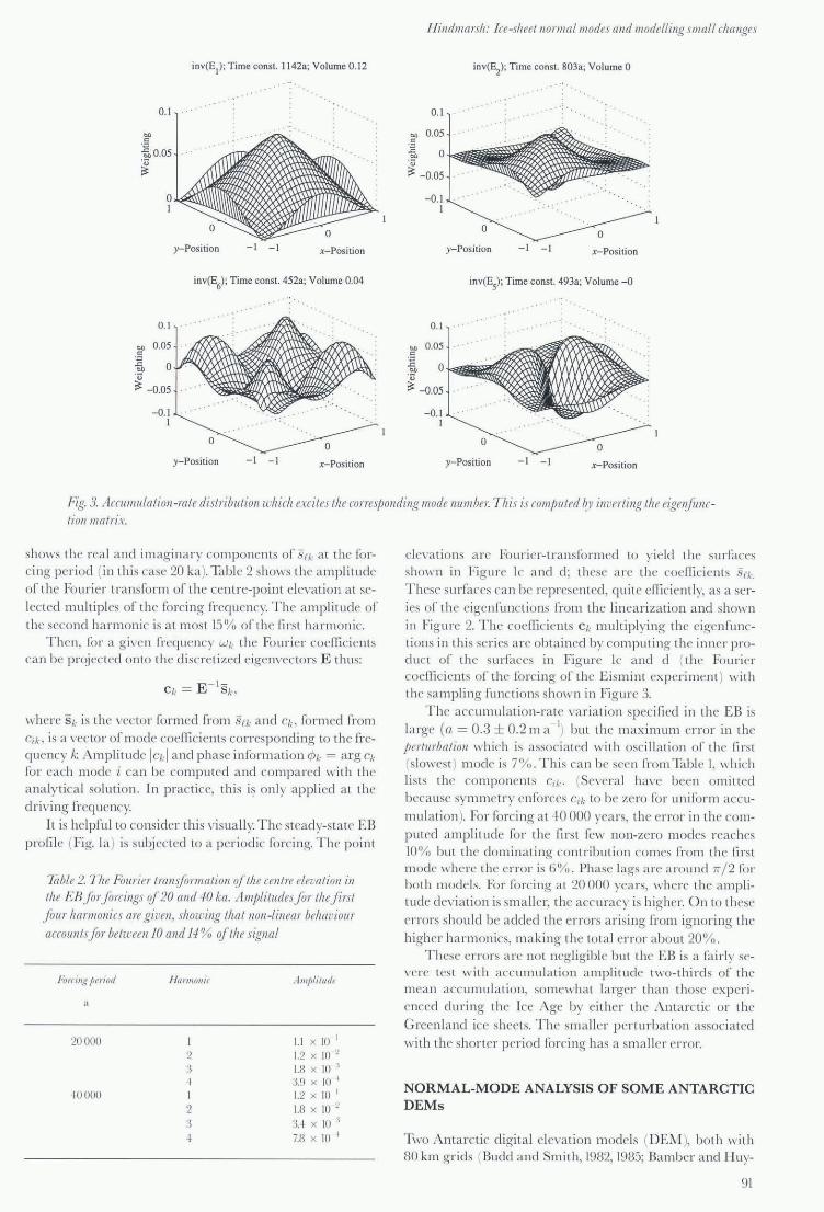
Fig. 3. J/cCllll1l1latioll -raLe disLributionll'li iC/z eleites the (o rresjJOlldillg //lode 11lImbn T his is comjJuted ~)I inverting LIL e eige7ifimc­tion l17(1 trir.

sholVS th e rea l a nd imaginary components or .5(k a t the ror­cing peri od (in thi s case 20 ka ). Table 2 shows the a mplitude

of th e Fo uri er transform of the centre-point eln'ati on a t se­

lec ted multiples of th e forcing frequency. The am plitude of the second harmonic is a t most 15% of th e first ha rmonic.

Then, for a g i\"Cn frequency Wk the Fouri er coeffi cients can be p roj ec tcd onto the disc reti zed eige nvec tors E thus:

where S k is th e \'ec to r formed from sn and Cb formed from Cik. is a \Tc tor of mode coeffi cie11ls corres ponding to th e fre­quency h.: Amplit ude ICkl and phase inform ati on cPk = a rg q.

fo r each mode i can be computed a nd compa red \\·ith the a na lytica l so lution. In practice, lhi s is onl y appli ed a t the

driving fi'equency.

It is helpful to consider thi s visua lly. The steady-sta te EB p ro file (Fig. la ) is subj ected to a pe ri odic fo rcing. The point

Table 2. The FOll rier transformation of the relliTe elevation in the £13 Jo rjorcillgs of 20 alld 40 ka. AlI/jJliLudes Jor Llle jirst jour harmonics are given, ShOll'illg LhaL !loll-linear behaviour a({Ollll /sjor be/ween lO and 14 % of/he signal

Fore i 1I,1.{ / ) ('1" iod

a

20000

"0000

Harm{)lIic

2 :3 .j.

I

2 3 .j.

. JIII/J/illlde

1. 1 x 10 I

1.2 x 10 ~ 1.8 x 10 ·' 3.9 x 10 I

1.2 x ID I

1.8 x 10 ~

:H x 10 1

I.R x 10 I

eleva ti o ns a rc Fo uri er-transform cd to yield the surfaces sholV n in Fig ure le a nd d ; th ese a rc lhe coe fficients .'ilk.

These surfaces can be represented , quite efTi cientl y, as a se r­ies of th e eigenfunctions from th e linea ri zation a nd sho\\'n in Fig ure 2. The coeffi cients Ck multipl ying th e eigenfunc­ti ons in thi s se ri es a rc obtained by computing the inner pro­duct of th e surfaces in Fig urc le a nd d ( th e Fouri er coe f1i cients or lhe fo rcing of lh e Eismint ex periment ) with th e sampling fun cti ons shown in Fig ure 3.

The acc umul a ti on-ra tc va ri a ti on spec ifi ed in th c EB is la rge (Cl = 0. 3 ± 0.2 m a I) but th e m ax imum error in th e jJerlurbatioll \\·hich is associa tcd wilh osc illa ti on of the lirst (slowest) mode is 7% . This can be seen from Ta ble I, \\'hich li sts the components Cik . (Se\Tra l ha\"C been omitted because symmetry enforces Ci k to be zero fo r uniform acc u­

mula ti on ). Fo r forcing a t +0 000 years, th e error in th e COI11-

puted a mplitude for the fi rs t fe\\' non-ze ro modes rcaches 10'10 but the dominating contribution comes from th e firsl mode where the error is 6°/.). Phase lags a rc a round 7r / 2 for both mod els. Fo r forcing a t 20 000 yea rs, whcre the a mpli­tude dev ia ti o n is sm all er, th e acc uracy is hig her. On to these

er rors should be added th e errors a ri sing from ignoring the

higher ha rmonics, ma king th e to ta l er ror about 20 % . Thesc errors a rc not negligibl e but the EB is a fairly se­

\ T IT leSl \\'ilh acc umul a ti on amplitude t\\·o-thirds of the mean acc umul a ti on, some\\'h at la rge r th a n those ex peri­enced during th e Ice Age by either the Anta rctic or the

Greenla nd ice sheets. The small cr perturbati on associa ted

with th e short er period forcing has a sm a ll e r error.

NORMAL-MODE ANALYSIS OF SOME ANTARCTIC DEMs

Two Anta rctic digit a l eb ·ati on models ( DE~I ), both with 80 km g rid s (Bude! a nd Smilh, 1982, 1985; Ba mber a nd Huy-

91

Hindmarsh: Ice-sheet normal modes and modelling small changes

brechts, 1996) with associated g rids of basal ele\'ation and surface acc umulation ra te we re used. Ba lance fluxes were ca lcul ated a nd the norm al modes eomputed. These coa rse g rids were used because it is still a formidable computa­ti ona l task to eompute a ll the modes for finer g rids, and it seemed desirable to compute a ll the modes in smaller tes t cases rather than truncating a rbitrarily with finer g rids. Th e Ba mber and Huybrechts (1996) elevati on grid is more accura te than the Budd a nd Smith (1985) grid, but th ere is an is 'ue of the sensitivity of the slower modes to data uncer­ta inty. In both computa tions the acc umulation data from

Budd and Smith (1 985) a re used. Hindmarsh (in press ) has di scussed the robustness of one-di mensiona l (I-D ) perturba­tions to the ice-sheet equation. In thi s case, a Sturm Liou­ville equation is obta ined and the robustness of their spec tra to model (not solution ) perturbation is well understood (Pryce, 1993). While Sturm- Liouvill e forms cannot be

obtained in higher dimensions, the robustness property is expec ted to be mainta ined.

Ba la nce fluxes and norm al modes were computed in the manner described above using 1/ = 3, 1n = 5, co rres pond­ing to internal deform ation according to a Glen (1955) rheo l­

ogy. A puzzling feature was the presence of eigenva lues and

vectors with non-zero imagina ry pa rts. The non-zero pa rts of the eigenvalues were at mos t no more than a few per cent or the corresponding real pa rts. There a re several poss ibl e causes fo r thi s but, if one considers the ice-sheet equ ation in the I-D fo rm

and expand s:

Ot H = C(8 - br' o.r (l oJ81"- 10.r8) +

m ( 10./:81"-10,.8) ( C(8 - br' - 1) (0.t8 - OJb) + a.

then, if loJ bl » 10.rsl,

o/H = - m(18csl'I-18rs ) (C(s - b) IIl - l ) 8.r b + a,

which is a first-order hyperbolic equ ation. In such a case, one is less surprised to see complex eigenvalues and they may therefore arise from rugose basal topography. The a rgument of the eigenvalues (i.e. Im(A)/R e(A)) is plotted in Figure 4. Complex eigenvecLOrs onl y occur when com­plex eigenvalues exist. Figure 4 shows that this problem onl y exists [or higher-mode numbers. The following di scussion refers to the real parts of the modes.

The six slowest modes for each case are shown in Figures 5 and 6, toge ther with associated ti me consta nts and vo­

lumes relative to the slowest mode. The res ults are broadl y simil a r a nd the percentage differences between the com­puted time constants a re sma ller than the uncerta inty in the rheological indices 1/ and m.

1\ significant result is that these low-order modes are smoo th, despite the use of accurate data in the MSSL data­se l. Thus, the process of computing the normal modes in d lcct filters the data in the sense tha t small-sca le spatial va r­iati on is onl y excited by small-scale forcing.

The e modes are clea rl y Eas t Anta rctic modes and

relate to the fac t that the time consta nts for East Antarctica are g reater than for\Vest Anta rctica owing to the low acc u­mula ti on rates (e.g. Hindma rsh, 1990). Evidentl y, the La mbert Basin splits the glaciodynamic response or East Anta rcti ca asunder. The tempta ti on should be resisted to

92

40

30 oil .,

-0 20 .:: ., ::l

lO c;; > c: ., 01l 0 '0

.I ~ ....

0

c-LO ., E ::l

~-20

-30

102

Mode number

Fig. 4. The argument of th e eigenvalue plotted against mode number. Non -zero mgllments me a lIumerical artifact. T he.)1 do not ajJ/Jear in modes qf < order 100.

conclude that coarsc g rids a re sufficient to compute the nor­ma l modes of an ice sheet. The a na lys is of Budd and' Va rner

(1996) shows how fl ow is directed into streams and it ca n be seen [rom the perturbati on Equa ti on (11) tha t spa ti al va ri a­ti ons in the zeroth-order di scha rge might well have a signif­icant effect.

The accumulation-rate sampling distributions (i. e. the rows ofE- i ) a re shown in Figure 7. Their spatial structure

is broadly simila r to the modes, as is the case in IHD (Hind­ma rsh, in press ), but owing to their non-orthogonality, do not excite only the corresponding mode, as compa red to the orthogonal fun cti ons that appear in IHD.

Volumetric spec tra (i.e. the eigenfunction volume

plotted against its associated time constants) a re shown in Figure 8. The slowest modes have time-steps of around 10000 yea rs, which can be predicted from the scale rela ti on­ship H / a(2n + 2) . The volumetric spectrum indicates the relaxation time-scal es of volumetric significance. The modes with short time constants do, in sum of absolute mag­nitude, represent a considerabl e volume but these modes a re assoc iated with spatial leng th scales smaller than likely \'ari a­ti on in the acc umulation rate and will not therefore be ac ti­\'ated significantly. Thus, most of' the \'olumetric response

ToNe 3. The amplitudes ofsome sjJatial modes in the EB con ­figurationfor forcings of period 20 and 40 ka, compared with the linear solutions. The linear amplitudes depend on thefor­cing period but the @ec/ is too small to be seen at the quoted aCCll raC)1

.lfode lIumber

a

20000 1 6 13 17

HJOOO 1 2 3

.I lode amplilude Ior /illfllr so/ulioll

2.1 0.28 0.099 0.089 2.3 0.2fl 0.0')')

0.089

LillenrampLilude EB amp/ilurle

1.0 0.93 1.06 0.92 0.93 0.90 0.96 0.90

Hin dll1aJ:fil: Ice-sheet norma! lI10des and lIIodelling smalf changes

70r-----------~------__.

20 40 60

M: T = 5976a 4 c

70,---------------------.

20 40 60

70 ,----------------------,

20 40 60

70,----------------------,

20 40 60

M : T = 6109a ) ,

70,----------------------,

20 40 60

70,----------------------,

20 40 60

Fig. 5. Si"( slowest modes colllplItedJrom tlte JllSSL dataset ( Ball/ber alld Hl~ybrec/lts, 1996). Associated tillle COIIS/all/S and relative volllmes are indicated. COII/ollr intervaL 0.2; black and white cOlltOllrs are rifoJ)posite sign.

seems to be concentra ted between 1000 a nd 10 000 yea rs. This is consi ·tent with concl usions obtained by Hu ybreehts (1992) using a non-linear thermomechanically coupled model.

It is possible, using the procedure described in Equations (18) to (20), to compute the response or the ice shee t to cha nges in the accumulat ion rate. The eigcnfunctions can

be Llsed to decompose the spat ia l distribution of the aCCLl­mulation and the evolution sp lit between fast , sla\'ed modes (with high wave-number spatia l \'ariability) the instanta­neous contr ibution or \\'hich is described by Equation (18a ) and the slo\\', large spatia l-sca le modes the evo lution or which is described by the dynamical Equation (19). In this

M1:Tc =989Ia M

2: Tc = 80 14a M): Tc = 5845a

70 70 70

60 60 60

50 50 50

40 40 40

30 30 30

20 20 20

10 10 10

20 40 60 20 40 60 20 40 60

M4

: Tc = 5534a Ms: Tc = 4834a M6: Tc = 4408a

70 70 70

60 60 60

50 50 50

40 40 40

30 30 30

20 20 20

10 ID 10

20 40 60 20 40 60 20 40 60

Fig. 6 Si.\ sLowest III 0 des compu/edJrom t/ze C II dataset ( Blldd and others, 1982). Associated time collstallts and reLative voLumes are indicated. Contollr intervaL 0.2; black and white contollrs are rifopposite sign.

93

Hilldmarsh: Ice-slzeelllormal modes and modelling small changes

M l: Tc= 10650. M2: Tc = 8 194. M3: Tc = 6 109.

70 70 70

60 60 60

50 50 50

40 40 40

30 30 30

20 20 20

10 10 10

20 40 60 20 40 60 20 40 60

M 4: Tc = 5976a Ms: Tc = 4980. M6: Tc = 4685a

70 70 70

60 60 60

50 50 50

40 40 40

30 30 30

20 20 20

10 10 10

20 40 60 20 40 60 20 40 60

Fig. 7 Distribution if accumuLation that opt/maL£)! ncites the corresponding mode, MSSL datasel.These accumulation distribu­tions will excite other modes as they are not orllwgonal. Contollr interval 0.2; black and while contoll rs are ofopposite sign.

Volumetric relaxation spectrum for Antarctica

101

104

e-folding time constant/a

Fig. 8. Volumetric spectrum: mode volume ploued against the associated time constanl. j\;fSSL da la pLolted ill heav} line, UM dataset il7 dotted line.

way, the spati a l structure assoc iated with the fas t modes can be reta ined in the evolution ca lcula ti on. In non-I inear models, data inconsistencies assoc ia ted with th e fas t modes tend to cause numerica l problems (c.g. O eri emans and Van der Veen, 1984) a nd data inconsistencies a re rel axed out by

running the model. Space limita ti ons preelude further dis­cuss ion of thi s important applica ti on.

CONCLUSIONS

Of th e three options discussed (o r initi a li zati on, the eas ies t one, which uses obse rved elevations in the zero th-order solution, seems to be a feasible way o[ initi a lizing models.

94

This is because the sma ller-sca le structure in the zeroth­order solutions is not manifested in the low-order modes of the perturbed solution. The practical consequence of thi s is high acc uracy. Normal-mode anal yses permit sma ll spati a l structure to be retained in models without being relaxed out, where it is due 10 data inconsistency or causing numer­ical instability. There remains a probl em of how to deal with sink holes.

The normal modes of two Antarctic DElVIs have been computed. The differences in eleva tion cause relatively small va ri ations in the spectrum and the qua lita tive features of the eige nfunctions remain simila r [or slower modes. The e-fo lding relaxa ti on time cons ta nt fo r East Anta rctica is a round 10 000 yea rs. The volumetric aspec t orthe rel axation of Anta rctica has been computed, with the most significant

response occurring on time-sca les between 1000 a nd 10000 years. \ Vha t causes the spati a l structure of the modes is not obvious a nd requires furth er il1\·estigati on. Better physics, in pa rtic ul a r the representa tion of g rounding-line motion a nd o[ sliding, should be available in the future.

ACKNOWLEDGEMENTS

I had instructive conversa ti ons with]. Bamber, \v. Budd, C. R aymond , D. Sorellsen, R . VVa rner and E. \Vadding ton. ]' Bambcr a nd R . \ Va rner prov ided me with da ta se ts ror Ant­arctica. G. K. C. Cla rke's review made me rethink th e struc­

ture of the paper.

REFERENCES

Bamber. J. L. and P. Huybrechts. 1996. Geomet ri c boundary cond itio ns for

modelling the ,"cloeit y fl d d of the Anta rctic ice shee t. .11111. Gtariol. . 23, 36+ 373.

Budd, W, F. a ndl. X Smi th. 1982. La rge-sca le nUlll cri ca llllode lli ng of the ,\ nta re li c ice shee t. . 11111. Glariol .. 3, +:2 1·9.

Bucle!. \\'. F. and 1. 1\. Smi lh , 1985. The Sla le of ba lance of Ihe ,\ ntarctic icc

sheet. III Glo('iel'l, ia Jilee/1. alld sea leI,eI: eU'erl a/a COl -illduced dillwlir rhollge. HellOrl 0/0 " orkJhojJ hdd ill Smllle, " ashillgloll, SelJil'lllbfl' 13 13,198·1. \ \'as hing­ton, DC, CS Departmenl of Enl'l'gy. O l1ice of Energy Research. 172 177. Report DOE/ ER/6023.1-1. ,

Budd. \\ '. F a nd R. c:. \\·arner. 1996 .. \ compulCJ' scheme IClI' rapid calcu la­lio llS ofbala nce-Il ux d islr ibu ti ons .. 11111. Clo[;oI.. 23. 21 27.

Budd, \\'. F , T. H. ,J acka, D.Jenssen. C. Rado k a nd ".\\'. l oung. 1982. f)eriml jJI!J'lirnl rhorar'eri."in o//he (" rfflllalld ice lheel. ,lIark I. Park\· ill e. \ 'inoria.

Ullin'rs il y of .\[dbourtlc . .\lcleorology Department. Publical ion 23. Chatdi n. F. 199:,. Eigelli'nlufJ q/malrirl'.I. C hichesler, \ \ 'iley a nd Sons. Dale\'. R. 1992 . . I/IIIOf/lhf'l'ir dolo (lI/aiJ'li,. Cambridge, Cambridge l 'n i\'('\'s ity

Press. Drl'\\'r)'. D.J. a nd E. :\1. .\ Ior ris. 19')2. The response of large ice sh'Tts to

cl ima ti c cha nge. Phi/u.'. 'li·all". R. SOl'. Llllldoll, SI'!: B. 338 (\28,; " 23.; 2+2. Fowler, A. C. 1992. i\lode lling ice , hcc t dyna mics. Ceopl!I '" . . 11'/rojJiI)'J. Fluid

I~)'II., 63 11 +). 29 66. Gle ll . ]' \\ '.1955. The creep ofpol\-crys tall inc ice. Pror. H. Sor. LOlldoll . Sf/: . 1,

228 1175. SI9 ,)3R. Go luh. C. H. a ncl c:. F. \'all Loall. 1989 . . I/r,lr;\ rOllllllllal;oll'. S('('olld 1'(1;1;011.

Baltimore, :\ I D, J ohn Hopk ins Prl'S>. H inclma rsh. R . c:. ,\ . 1990. Time-sca les and degrees o ri'reedom operat ing in

lhe c\'()lution ofcominenta l ice-sheets. 7iwlJ'. R. Soc. Edillb/lrgh, Earllt Sci., 81 +,371 38+.

H indma rsh. R . C. .\ . 1992. Est imati ng ice-shect respollSC' to climate chan!\,c. III .\lorris, E. i\1.. ed. COlllribulioll '1/ . llIlorrl;c Penill,wla i(e 10 \ea lel'd ri,e. Rej)(JI'I ji,,. Ihe COIIIIII;. ,';UII IJ! Ihe EUfOpeall CO/l//l/ulI;l;e< Pmj""1 I,POC-( 7 91) ­I){)fj. Ca mbri dge. Bri tish Anta rctic SU ITCY, 27-3·f.

H ind m ars h. R. c.:. A, 1996a. Stabilit y or in' rises a nd UlIl'oupled marine ice sheets .. 11111. Glaciol .. 23. 105 115.

H indmarsh, R. C. .\ .1996b. StochaSlic perturbation of'cli\'iclc position . . 11111.

Glacial .. 23.9+ 10+. H indtnarsh. R . C. .\ . In press. " ormal modes ofan ice shec t. ] Fillid .Iferh .. I-l ind marsh. R . c.:. ,\. a nd A.J. Pa), nc. 1996. Time-step li mi ts 101' stable solu­

tio ns of thc ic(' -sl1<'ct cq ua ti on . ..11111. Glnr;ol., 23, 7+ R5. H ll tt er, K. 19R3. 7 heorel;(al .~/a(;%gJ': lIIaln;,,1 ,I(;ell(e o/;re alld Ihe lIIedwII;CI 0/

Hillrilll(fl1h: k e-shee/ normal modes and modelling sm(fll changes

glacim alld i(e 1/II'ell. Dorclrecht, etC'., D. Reick l Publishing Co.ulkyo.

Thra Publis hing Co.

H u),brechts, P. 1992. T he AmarCl ic ire shee t a nd ctl\·iro nll1enta l change: a three-cli nl('ns iona l mode ll ing study. Bel: Pola~jilrsch. ~)9.

Il lIybrcchb. P .. T. Paync and the EIS:\II "T I tllel'Cotll lxlrison Gro up. 1996. T hl' EIS:\ ""T benchmarks 101' testing icc-sh(,ct models .. 11111. Glar;ol .. 23.1 1+.

,J6hann('s50n. T. 1992. T he la ndscapc of lemperate ice ca I". Ph. D. thes is. l'n i\'crsi l y of\ \ ·ashing ton.

:--lorl ancl. L. \ \ '. IClA·k T hermolllechanica l balances or ice sheet l1 o\\'s.

(;eollhl'l . . "'lOpl!)'\. Fillid l~J'II .. 29. ~37 266. ")'<' . .J. F. 1952 .. \ lIlethod ofcairu lating Ihl' thic kn ess ofiee sheets . . \ itlllre.

169 4300 .. 129 .YlO. "yc. J. F 1').)9. The mrnion of in" ,h(,(,h and ~laci(T'.] (;Iar;ol., 3 26. +9:1 .)07. Oeri ema ns . .J. 19HI. Ell t'Cl or irregu lar ll uClua ti ons in i\n ta rCl ic precip ita­

ti on On globa l sca 11'\'('1. ,\ a/llre. 29015809). 770 772.

Onlcma ns. J. ancl C . .J. \ 'an del' \ '('CIl, erl.l. 198-1. Ire "Ited' ({lid dill/a/e. Dordrechl. Cle .. D. Reide l Publish ing Co.

Paylll'. .\ ,.J. 199.'>. l. im it {'\Tics in the b",a l thcrmal rl'~ i me or ice shccls.] (;,'o/J/m. RfJ .. 100 13 :; . -12+9 +26:1-

Pr)ce, .J. 1993 .. \;/ll/er;1'01 w/ul;oll ~/Sllll/II L;(JlI1'I'II" Ilmbiellll. Ox lord. Oxlc)I'cl L ni\-C' rsil Y Pn:ss.

Ri- my. F .. c.:. Ritz and 1.. Brissl't. 19%. Ire-sheet no\\' Icat ures and rheo logical

paramelcrs dni\'Cd I'rom prec ise allilllc tric topography .. 11111, Glacial .. 23. 277 281

S()ITmcn. D. 1992. Implic it applicat ion of poh-nomial filters in a k-, tl'P .\ rno lcli Illet hod. SI. l.lf ].\I({/r .. 111111 . . Jfi/1I .. 13, :,57 385.

\ 'an der \ 'cell, C . .]. 1993. In tcrpre tation nr sho n -tilll\' ice-shee t dc\'ation cha nges in it-rrcd Il'om sa te ll it" a lt ime t ry. Clill1al;r (;/wllge, 23 1,. 383 -10:).

\ 'i"IO\·. S. S. 19,)8. Regu lar ities of icl' clclormation ,,,nl(' resu lts of lalJorat()lY

researches. IlIlm/{//iolla! . IIIori({lion of Srienli/ir f{J'drologr Pllblica/ioll +7 Symposi um al Chamonix 19.')8 1'1!I'sinlJ!lhe .\lowllelll a/lite Ire, 383 391.

\ \ 'e[,rllllan, .J. 1957. O n the sliding of glaciers. ] C/ruiol., 3 21 .33 38. \\ ·i lki"son . .J. R. 19G.i The fl!~"'Jr({;r £.I:~ell('{/Iue Pro/J/l'lI1. Oxl()rd. Oxli)l'(l

U ni\ 'crs il y Prl's~.

95