use of fragile geologic structures as indicators of ...bakerjw/publications/baker_et_al_(2013... ·...

Use of Fragile Geologic Structures as Indicators of Unexceeded

Ground Motions and Direct Constraints on Probabilistic

Seismic Hazard Analysis

by Jack W. Baker, Norman A. Abrahamson, John W. Whitney, Mark P. Board,and Thomas C. Hanks

Abstract We present a quantitative procedure for constraining probabilistic seis-mic hazard analysis results at a given site, based on the existence of fragile geologicstructures at that site. We illustrate this procedure by analyzing precarious rocks andundamaged lithophysae at Yucca Mountain, Nevada. The key metric is the probabilitythat the feature would have survived to the present day, assuming that the hazard re-sults are correct. If the fragile geologic structure has an extremely low probability ofhaving survived (which would be inconsistent with the observed survival of the struc-ture), then the calculations illustrate how much the hazard would have to be reducedto result in a nonnegligible survival probability. The calculations are able to considerstructures the predicted failure probabilities of which are a function of one or moreground-motion parameters, as well as structures that either rapidly or slowly evolvedto their current state over time. These calculations are the only way to validate seismichazard curves over long periods of time.

Introduction

For critical facilities, seismic hazard needs to be com-puted for ground motions with annual rates of exceedanceof 10−6 (for nuclear power plants) to 10−9 (for nuclear wasterepositories). At these low exceedance rates, very largeground-motion amplitudes are often predicted by standardprobabilistic seismic hazard analysis (PSHA) procedures.This is in large part because ground-motion amplitudes fora given earthquake appear to be well represented by lognor-mal probability distributions, and extrapolating the lognor-mal distribution to a high number of standard deviationsassociated with extremely rare ground motions results inextremely large amplitudes. Because the lognormal distribu-tion has no upper bound, there is no absolute upper bound tothe ground-motion amplitudes that can be computed at verylow probabilities.

An example of how these extreme ground motions arisein a standard PSHA is the 1998 Yucca Mountain ProjectPSHA (Stepp et al., 2001). The hazard curves for peakground acceleration (PGA) and peak ground velocity (PGV)in Figure 1 show progressively higher ground motions asthey are extended to progressively lower rates of exceedance:at mean hazard levels of 10−6=yr, 10−7=yr, and 10−8=yr, thecorresponding PGAs are 3, 6, and 11g (Fig. 1a) and corre-sponding PGVs are 3, 6.5, and 13 m=s, respectively (Fig. 1b).These extreme ground motions, the consequence of extrapo-lating ground-motion distribution functions to extremely low

probability levels, have generated considerable consternationin the scientific, engineering, and regulatory communities:the upper end of these PGVs and PGAs has never been re-corded for earthquakes, present exceptional challenges tothe design and construction of facilities, and are regardedby many seismologists as “physically unrealizable” (e.g.,Andrews et al., 2007). These extreme PGV levels may beunrealizable because the amplitude of the ground motiontraveling through a rock mass is limited by the shear strengthof the rock mass through which it propagates. It is easy to saythat the large ground motions predicted at low probabilitylevels from the 1998 PSHA do not seem reasonable, but itis much more difficult to provide a technical basis for a re-duced ground-motion value.

One source of evidence for a reduced ground-motionvalue comes in the form of fragile geologic structures suchas precarious rocks, which would likely have been destroyedby seismic ground motions if the PSHA calculations are cor-rect. Precarious rocks, also precariously balanced rocks(PBR) have been used as constraints on local ground motionssince Brune and Whitney (1992) and Brune (1996) recog-nized PBRs as natural seismoscopes. PBRs are a subset of themore general class of fragile geologic structures (FGS),which speak to unexceeded ground motions (UGM), groundmotions that would have damaged or destroyed any object,structure, or feature during the time in which it was fragile.

1898

Bulletin of the Seismological Society of America, Vol. 103, No. 3, pp. 1898–1911, June 2013, doi: 10.1785/0120120202

Such FGS include natural bridges and arches, liquefiabledeposits, hoo-doos, precipitous slopes and cliffs, and litho-physal cavities, as well as PBRs. Lithophysae (delicate voidsand crystals in welded vesicular tuff–literally, rock bubbles)are the result of gases exsolving from cooling lava flows andashfall tuffs. PBRs are the most important of the FGS becausethey occur widely across active tectonic terrains of the south-western United States (e.g., Brune, 1996; O’Connell et al.,2007; Purvance et al., 2008) and elsewhere in the world (e.g.,Stirling and Anooshehpoor, 2006).

When used as a constraint for PSHA, one needs to knowthe “fragility age” of the FGS of interest (i.e., the amount oftime it has been in its presently precarious/fragile state) aswell as the ground motions that, had they occurred, wouldhave damaged or destroyed it. Early work used the presenceof desert varnish on PBRs to indicate fragility ages of thou-sands of years or greater and quasistatic estimates of topplingaccelerations to approximate a PGA that had not occurred inthe fragility age of the PBR. As recounted in Anderson et al.(2011), techniques for estimating both the fragility ages andtoppling motions have advanced considerably in the past de-cade to include cosmogenic dating of features (Balco et al.,2011) and numerical modeling of dynamic toppling behavior(Purvance et al., 2009).

The Points-in-Hazard-Space approach and graphic de-veloped in the course of the Extreme Ground Motions re-search program (Anderson and Brune, 1999; Abrahamsonand Hanks, 2008; Hanks and Abrahamson, 2008) allowsone to compare PBR constraints directly with seismic hazard

curves, the specific place and application being YuccaMountain, Nevada. Reciprocal fragility ages were used to ap-proximate the probabilities of nonexceedance of estimates ofPGV that would have toppled the PBR, had they occurred.This simple approach, although effective in demonstratingthat the seismic hazard at Yucca Mountain had been signifi-cantly overstated, lacked the quantitative probabilistic frame-work we develop in this paper.

This paper provides a description of the types of evi-dence that have been compared to PSHA results and describesa probabilistic procedure for performing such comparisons.The proposed calculations can incorporate uncertainty in theage and fragility of the observed geologic structure, so as tobe consistent with other uncertainties used to perform theinitial seismic hazard analysis computation.

Seismic Hazard Analysis

Standard PSHA is performed using a seismic sourcecharacterization that describes the rates of occurrence of allearthquake events in the region and using a ground-motionprediction model to predict the distribution of ground-motionintensities for each earthquake event. Those two models cap-ture inherent physical variability (“aleatory” variability) inthe processes that generate ground motions at a given site.We do not have perfect seismic source characterizationmodels or ground-motion prediction models, however, sotypically a logic tree is used to describe our lack of knowl-edge (“epistemic” uncertainty) in the proper model by pro-posing a list of plausible models via a logic tree, along with

1

10–8

10–7

10–6

10–5

10–4

10–3

10–2

10–1

1

10–8

10–7

10–6

10–5

10–4

10–3

10–2

10–1

(b)(a)

0.1 1

Data Tracking Number MO03061E9PSHA1.000 Data Tracking Number MO03061E9PSHA1.000

Mean

5th Fractile

15th Fractile

50th Fractile (Median)

85th Fractile

95th Fractile

Mean

5th Fractile

15th Fractile

50th Fractile (Median)

85th Fractile

95th Fractile

10 100 1000 100000.10.01 1 10 100

Horizontal peak ground velocity (cm/s)A

nn

ual

pro

bab

ility

of

exce

edan

ce

An

nu

al p

rob

abili

ty o

f ex

ceed

ance

Horizontal peak ground acceleration (g )

Figure 1. Example output from probabilistic seismic hazard analysis. (a) Horizontal PGA, and (b) horizontal PGV, at Point A, a hypo-thetical, reference rock outcrop site at the Yucca Mountain repository horizon (Stepp et al., 2001). From the 1998 Yucca Mountain ProjectPSHA extended to 10−8=yr by BSC (2005). The color version of this figure is available only in the electronic edition.

Fragile Geologic Structures as Indicators of Unexceeded Ground Motions and Direct Constraints on PSHA 1899

weights representing our degree of belief in each model(SSHAC, 1997; Abrahamson and Bommer, 2005; McGuireet al., 2005).

The output of such a calculation is a plot (as shown inFig. 1) that shows mean hazard curves and fractiles for PGAand PGV. An important feature of these calculations is thatthere is generally no upper bound on the ground-motion pre-dictions, so there is no fixed upper limit on the amplitudes ofpredicted ground motions (although large amplitudes may beextremely infrequent).

Potential Constraints on Hazard Curves

Three general types of constraints have been proposedto constrain PSHA predictions of large ground-motion in-tensities: physical limits on ground motion, truncation ofground-motion predictions, and unexceeded ground motionsassociated with fragile geologic structures (Hanks et al.,2006).

A physical limit to earthquake ground motion is a con-straint such that motions larger than this limit cannot occurever. Such a limit, if it can be plausibly demonstrated andcalculated, provides a clear bound on extreme ground mo-tions. Physical limits might arise from the limited strengthof rocks at the site of interest or anywhere along the pathbetween the rupture and the site. The strength of rocks in-creases with confining pressure, so we may expect that rockproperties at or near the site will place more stringent limitson ground motions than will rock properties at midcrustaldepths, where the earthquakes occur. Moreover, rocks atshallow depth are easily accessible, allowing for both in situobservation of their structure and fabric as well as samplingfor laboratory testing. Rock mechanics can then be used toidentify limits at which rock fracture would occur (BSC,2005, Section B.2.2; Lockner and Morrow, 2008). Physicallimits to ground motion might also arise from limits on thesource excitation of crustal earthquakes, but these are diffi-cult to discern with confidence given the inaccessibility ofearthquake sources and the short record of instrumental re-cordings. A related approach is to identify a hard limit onintensities that have zero probability of being exceeded underany condition using numerical simulations, a challengingbut feasible approach (Andrews et al., 2007). Physical limitsdo appear to provide useful constraints on extreme groundmotions, but are not addressed further here.

A second potential approach to constrain hazard is totruncate predictions of ground motions at a fixed numberof standard deviations (“epsilons”) above the median predic-tion for a given earthquake scenario. This approach is prob-lematic because the truncation point is arbitrary and notsupported by observational evidence and because the trunca-tion is with respect to a model prediction rather than withrespect to an absolute ground-motion intensity value wheresome physical phenomenon produces the truncation. Theproblems with this approach are described in detail by

Bommer et al. (2004), and thus this line of thinking has notproduced defensible constraints on extreme ground motion.

A third approach is to use the existence of a fragile geo-logic structure as an indicator that ground motions with am-plitudes large enough to fail the structure have not occurredduring its lifetime. Examples of features that indicate unex-ceeded ground motions include undamaged lithophysae(rock bubbles) and precariously balanced rocks. Althoughthese observations provide clear qualitative evidence, severalchallenges are associated with using them for quantitativecomparisons to probabilistic seismic hazard calculations.These challenges will be addressed below.

Using Fragile Geologic Structures to ConstrainHazard

FGS are indicators of UGM—ground motions strongenough to drive an FGS to failure but which have not oc-curred during the time period for which the FGS has indeedbeen fragile. These structures provide observations in a sin-gle window of time from the origin of the structure untilpresent, whereas hazard curves quantify long-term rates ofexceedance of ground-motion amplitudes. There is alsouncertainty in the amplitude of ground motion that woulddestroy those structures. For these reasons, it is not straight-forward to compute the UGM associated with an FGS.

To illustrate the proposed approach to address thesechallenges, we first consider the Topopah Spring tuff forma-tion that underlies Yucca Mountain and is the host horizonfor the underground repository. It consists of ∼300 m ofsilica-rich, densely welded, pyroclastic flow units laid down12.8 million years ago and contains distinctive upper(Tptpul) and lower (Tptpll) lithophysal units. Lithophysaeare cavities that form in pyroclastic flows and volcanic tuffsas a result of the volcanic gases exsolved during the coolingprocess but contained within the cooling rock mass. Thecooling occurred over a relatively short period of time com-pared to the age of the units, so the age of the lithophysae canbe taken as 12.8 million years without concern for the fra-gility varying over that time period.

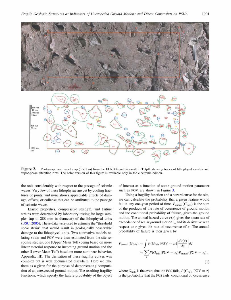
Tptpul lithophysae tend to be roughly spherical, uniformin size and distribution, and small in dimension (diameters of1–10 cm); the matrix material is largely unfractured. Tptplllithophysae are more irregular in shape, size, and distribu-tion, as seen in Figure 2. Lithophysae range in size fromabout 1 cm to nearly 2 m in dimension and have spacing thatranges from about 10 to 50 cm, although they may be moreclosely spaced in local regions. The shapes range from ellip-tical or spherical to irregular, cuspate and merged cross sec-tions, or elongate along fractures. The matrix betweenlithophysae often has a fabric of short length (<1 m) anddiscontinuous cooling fractures that have a primarily verticalorientation. These fractures typically are not interconnectedand do not intersect lithophysal cavities. The overall porosityof Tptpll due to the lithophysae is ∼20%, and these cavitiesconstitute 10%–30% of the rock volume, thus weakening

1900 J. W. Baker, N. A. Abrahamson, J. W. Whitney, M. P. Board, and T. C. Hanks

the rock considerably with respect to the passage of seismicwaves. Very few of these lithophysae are cut by cooling frac-tures or joints, and none shows appreciable effects of dam-age, offsets, or collapse that can be attributed to the passageof seismic waves.

Elastic properties, compressive strength, and failurestrains were determined by laboratory testing for large sam-ples (up to 288 mm in diameter) of the lithophysal units(BSC, 2005). These data were used to estimate the “thresholdshear strain” that would result in geologically observabledamage to the lithophysal units. Two alternative models re-lating strain and PGV were then estimated from the site re-sponse studies, one (Upper Mean Tuff) being based on morelinear material response to incoming ground motion and theother (Lower Mean Tuff) based on more nonlinear behavior,Appendix III). The derivation of these fragility curves wascomplex but is well documented elsewhere. Here we takethem as a given for the purpose of demonstrating computa-tion of an unexceeded ground motion. The resulting fragilityfunctions, which specify the failure probability of the object

of interest as a function of some ground-motion parametersuch as PGV, are shown in Figure 3.

Using a fragility function and a hazard curve for the site,we can calculate the probability that a given feature wouldfail in any one-year period of time. Pannual�Gfails� is the sumof the products of the rate of occurrence of ground motionand the conditional probability of failure, given the groundmotion. The annual hazard curve ν�z� gives the mean rate ofexceedance of scalar ground motion z, and its derivative withrespect to z gives the rate of occurrence of z. The annualprobability of failure is then given by

Pannual�Gfails� �Z

P�GfailsjPGV � zi��dν�z�dz

��dz�

Xi

P�GfailsjPGV � zi�Pannual�PGV � zi�;

(1)

whereGfails is the event that the FGS fails, P�GfailsjPGV � z�is the probability that the FGS fails, conditional on occurrence

Figure 2. Photograph and panel map (3 × 1 m) from the ECRB tunnel sidewall in Tptpll, showing traces of lithophysal cavities andvapor-phase alteration rims. The color version of this figure is available only in the electronic edition.


of a ground motion with PGV � z (the FGS “fragility func-tion”), and “j” is used to denote conditioning. The calculationcan be specified in continuous form as indicated by the in-tegral in equation (1), but in practice it is evaluated numeri-cally by discretizing the continuous range of PGV values ofinterest and summing over those values, zi. Figure 3 showstwo fragility functions for the lithophysal units, and Figure 4shows the Yucca Mountain mean hazard curve with respectto PGV. For this hazard and the Lower Mean Tuff fragilitycurve shown above, Pannual�Gfails� � 4:5 × 10−6=yr.

Given the above annual failure probability, the probabil-ity of surviving for one year is 1 − PAnnual�Gfails�, and theprobability of surviving for T years (assuming potential fail-ures in each year are mutually independent) is

P�Gnot failed� � �1 − Pannual�Gfails��T: (2)

For the hazard curve and Lower Mean Tuff fragilityabove, and a 12.8 million year age of the Tuff, this proba-bility is 10−25 or, for all practical purposes, zero. This contra-dicts the observed existence of the structure, suggesting thatthe hazard curve is overpredicting the rate of exceedance ofthe large PGV values that would cause failure of this FGS.The approach proposed here to reconcile such a contradic-tion is to multiply all rates of exceedance from the originalhazard curve by a constant α, so that if the original hazardcurve was ν�z�, the adjusted hazard is αν�z�. By inspectionof equation (1), we can see that this will modify the annualfailure probability of the structure by the same constant. Wecan, thus, determine the scale factor α to be applied to thehazard curve that would lead to a specified probability P1,for which our structure does not fail during its lifetime. Fora structure that has been fragile for T years, P1 is

P1 � �1 − αP1Pannual�Gfails��T: (3)

If we are interested in the hazard curve that would leadto a 5% probability of the FGS not failing, we can substituteP1 � 0:05 and solve for the corresponding αP1

α0:05 �1 − 0:051=T

Pannual�Gfails�: (4)

For this example, α0:05 � 1=19, Figure 4 shows the re-sulting scaled hazard curve as a dashed line. For any hazardcurve above this scaled hazard, there is <5% chance thatthe geologic structure would have survived in its existingstate of fragility for T � 12:8 million years. The 5% targetis a choice in this analysis and is addressed in the Discussionsection below.

We can further analyze the results from the calculationsabove to identify which particular PGV values are contribut-ing most to failures of the structure. The product of the rate ofoccurrence of a given PGV and the corresponding fragility(the integrand of equation 1) provides the contribution ofeach PGV to the total failure probability of the fragile geo-logic structure. These contributions are computed as followsand plotted in Figure 5a

P�Gfails due to PGV � zi�

� P�GfailsjPGV � zi�Pannual�PGV � zi�Pannual�Gfails�

: (5)

We can also compute the cumulative contribution of allPGVs ≤ z to failure, which is computed as follows and plot-ted in Figure 5b

P�Gfails due to PGV ≤ z�

�Pz

zi�0 P�GfailsjPGV � zi�Pannual�PGV � zi�Pannual�Gfails�

: (6)

0

0.2

0.4

0.6

0.8

1

PGV (cm/s)

P(G

fails

| P

GV

= z

)

material properties

material propertiesUpper Mean Tuff

Lower Mean Tuff

10050 500 1000

Figure 3. Fragility curves as expressed by the Upper and LowerMean Tuff properties. The color version of this figure is availableonly in the electronic edition.

10–8

10–6

10–4

PGV (cm/s)

Ann

ual r

ate

of e

xcee

danc

e

Mean hazardα*(Mean hazard)

UGM

Range of 25% to 75% contribution

10050 500 1000

Figure 4. Original mean hazard curve for the site and adjust-ment of hazard curve to correspond to a 5% survival probabilityof the lithophysae. The color version of this figure is available onlyin the electronic edition.


The median of the PGVs contributing to failure, denotedz1, is taken as the UGM for this fragile geologic structure.The 50th percentile cumulative failure probability point onthe scaled hazard curve fixed by z1 is the PGV most stronglyconstrained by the fragile geologic structure. This z1 value isshown in Figure 4, along with a solid red segment of thescaled hazard curve indicating the range of PGV that coversthe 25%–75% range of the failure probability in Figure 5b,revealing that the fragile geologic structure constrains onlypart of the hazard curve (this range is chosen to illustrate thatthere is not just a single PGV value for which the FGS is pro-viding some constraint). This point tells us the following: ifthe hazard curve passes through this point, then there is a 5%probability that the structure would survive T years withoutfailing, and this is the median of the PGV values that wouldcause failure of the structure.

The relative values of z1 and the point of 50% probabil-ity of failure depend on the slopes of the hazard curve and thefragility curve. Typically, z1 is lower than the ground motionat the 50% failure probability because there are so manymore small earthquakes with smaller ground motion; eventhough the fragility is low, the rates of the smaller PGVs aremuch higher than the rates of ground motions correspondingto the 50% failure probability on the fragility function. If thefragility curve is steep (e.g., the fragile geologic structure isbrittle), then the z1 value will be close to the value that leadsto a 50% chance of failure because the fragility for the lowerground-motion values will be very small, offsetting the higherrate of occurrence of the smaller ground-motion values.

With this approach, the absolute level of the originalhazard curve does not affect the location of the UGM. If twohazard curves differ only by a multiplicative factor on theirrates (i.e., they have the same shape), then z1 as determinedby this method is unchanged and α simply adjusts for thedifferences in levels of the original hazard curves. The loca-tion of the UGM will depend upon the slope of the hazardcurve, however, as the slope tells us the relative rates of largeand small PGV, and differences in these relative rates willaffect the PGV values that most constrain the hazard curve.

As an example of the dependence of the UGM point onthe hazard curve, the UGM is shown for three different PGVhazard curves in Figure 6: mean, 95th fractile, and 5th frac-tile. For the mean and 95th fractile hazard curves, the shapesare similar and so there is almost no change in the locationof the UGM. For the 5th fractile, the slope becomes muchsteeper, indicating that large PGV values are predicted tobe very rare, so z1 becomes smaller as the smaller PGVs thusprovide the stronger constraint. The UGM based on the 5thfractile hazard is shifted up and to the left. All three pointsfall along a line following the general slope of the hazardcurves, indicating that in all three cases the FGS providesa consistent evaluation of the hazard curve. Note that the

10050 500 50 z1 500100010–3

10–2

10–1

PGV (cm/s)

P(G

fails

due

to P

GV

= z

)

P(G

fails

due

to P

GV

≤ z

)

100 10000

0.25

0.5

0.75

1

PGV (cm/s)

(b)(a)

Figure 5. (a) Contribution of PGVs to failures of the feature. (b) Cumulative contributions of PGV ≤ z to failures of the feature. The colorversion of this figure is available only in the electronic edition.

Figure 6. Effect of different slopes of the hazard curves on theUGM. The color version of this figure is available only in the elec-tronic edition.


5th fractile hazard curve lies below the UGM points, meaningthat the FGS would have >5% chance of surviving if it werethe true hazard curve. We note that fractile hazard curves arenot necessarily representative of actual hazard curves fromindividual logic tree branches, but these calculations none-theless serve to illustrate the role of the hazard curve slopeon UGMs. Further, Figure 4 illustrated that the UGM isconstrained by a relatively narrow range of PGV values forwhich the fractile hazard curve is likely similar to an indi-vidual hazard curve.

Fragile Geologic Structures with Vector Fragility

Many PBRs have been discovered and documentedon the west face of Yucca Mountain and elsewhere (e.g.,Brune and Whitney, 1992, 2000; Bell et al., 1998; Andersonand Brune, 1999; Purvance et al., 2008; Stirling et al., 2010).These features have great potential to constrain seismic haz-ard calculations, but two complications arise when one isused to compute an unexceeded ground motion: its topplingprobability is a function of both PGA and PGV, requiringknowledge of their joint probability distribution in a givenfuture ground motion, and the rocks evolve in shape over timeso that their fragilities are not constant over their lifetimes. Toillustrate how these complications can be addressed, we per-form an example evaluation of the PBR named Matt-cubed,located on the west face of Yucca Mountain. A photographof this rock is shown in Figure 7a, and its fragility curve isshown in Figure 8a, as determined by Purvance et al. (2009).The derivation of this fragility curve was complex but is welldocumented elsewhere. Here we take it as a given for the pur-pose of demonstrating computation of an unexceeded groundmotion.

This vector fragility causes a difficulty for the UGMcomputation because hazard curves provide the rate of occur-rence of a given PGA or PGV individually and not the rate ofjointly observing a given PGA and a given PGV in a singleground motion. To use the PBR toppling fragilities in the con-text of a UGM calculation, which considers PGV hazard only,we need to replace the functional dependence on PGA (whichwe do not know) with some equivalent information that wedo know.

To begin, we first convert the pairs of PGA and PGV/PGAvalues calculated by Purvance et al. (2009) into pairs of PGVand PGA/PGV values, with PGVas the abscissa, as illustratedin Figure 8. Each coordinate in Figure 8a has some corre-sponding coordinate in Figure 8b, and the two correspondingcoordinates have identical toppling probabilities. For agiven PGV value, Figure 8b now provides failure probabil-ities as a function of PGA/PGV; this is illustrated in Figure 9for PGV � 30 cm=s.

Earthquake seismologists will know that PGV has a strongmagnitude dependence (e.g., McGarr and Fletcher, 2007) andso does PGA/PGV, although less strong as we shall see shortly.So how does PGA/PGV depend on M? This is shown empiri-cally in Figure 10, which shows observed PGA/PGV valuesfrom ground motions on rock sites (VS30 > 500 m=s) at shortdistances (R < 20 km) from the Next Generation Attenuationdata set (Chiou et al., 2008). The mean value of ln(PGA/PGV)can be predicted as a function of magnitude using the follow-ing regression equation, which is also shown in Figure 10

E�ln�PGA=PGV�� 6:08 − 0:534M − 0:074�M − 6:07�2:(7)

There is not a significant trend in this data with distanceor VS30, so the regression equation is not dependent on those

Figure 7. (a) Photograph of PBR Matt-cubed. (b) Photograph of PBR Tripod. The color version of this figure is available only in theelectronic edition.


variables. The standard deviation of prediction errors fromthis equation is 0.49. Assuming that PGV/PGA for a givenmagnitude is a lognormal random variable, the probabilitydensity function (PDF) for PGA/PGV, associated with a givenmagnitude M, is then

fPGA=PGV�yjM�� 1

0:49y��2π

p

exp�−0:5

�lny− �6:08−0:534M−0:074�M−6:07�2�

0:49

�2�:

(8)

Figure 10 illustrates this PDF for M � 6 and M � 7.

Knowing the probability of failure of the PBR given aPGVand PGA/PGV pair, and the distribution of PGA/PGV val-ues given an earthquake magnitude, we can integrate over allpossible PGA/PGV values to obtain the probability of failurefor every PGVandM (at the close distances implicit in Fig. 10)

P�GfailsjPGV � z;M � m� �Z

P�GfailsjPGV � z;

PGA=PGV � y� � fPGA=PGV�yjm�dy; (9)

where P�GfailsjPGV;M� is a generalized form of the fragilityused in equation (1). These fragilities for the example rock areplotted in Figure 11 versus PGV for a range of magnitudes.This figure illustrates that large magnitude earthquakes require

0 5 10 15 200

0.2

0.4

0.6

0.8

1

PGA/PGV (1/s)

P(G

fails

|PG

V =

30

cm/s

, PG

A/P

GV

= y

)

Figure 9. Overturning probabilities for the PBRMatt-cubed as afunction of PGA/PGV, given PGV � 30 cm=s. The three pointsmarked with symbols on this fragility curve correspond to the pointswith the same symbols in Figure 8. The color version of this figureis available only in the electronic edition.

5 6 7 81

10

100

Magnitude

PG

A/P

GV

(1/

s)

Empirical data

E [ln(PGA/PGV)]

fPGA/PGV(y |M )

Figure 10. Scaling of PGA/PGV with magnitude for rock sites(VS30 > 500 m=s) at short distances (R < 20 km). The colorversion of this figure is available only in the electronic edition.

0 0.1 0.2 0.3 0.4 0.50

0.1

0.2

0.3

0.4

0.5

PGA (g )

PG

V/P

GA

(s)

10 10050 2000

5

10

15

20

PGV (cm/s)

PG

A/P

GV

(1/

s)

P(Gfails) = 0.1

P(Gfails) = 0.5

P(Gfails) = 0.9

(b)(a)

Figure 8. Overturning probabilities for the PBR Matt-cubed. (a) Plotted as a function of PGA and PGV/PGA. (b) Plotted as a function ofPGV and PGA/PGV. The color version of this figure is available only in the electronic edition.


higher PGVs in general to topple the feature because their PGAvalues (relative to PGV) are smaller than for small-magnitudeearthquakes with the same PGV.

This fragility function format is useful because we knowthe distribution of magnitudes associated with a given PGVvalue at the site from seismic hazard deaggregation calcula-tions (e.g., McGuire, 1995). Here we denote the deaggrega-tion probability that a ground motion with PGV � zi wascaused by an earthquake withM � mj as deagg�mjjzi�, not-ing that the deaggregation calculation typically discretizesthe continuous range of possible magnitudes. Using thisdeaggregation information and the magnitude-dependent fra-gility function of equation (9), we can compute the annualprobability of failure of the precarious rock using

Pannual�Gfails� �Xi

Xj

P�GfailsjPGV � zi;M � mj�

× deagg�mjjzi�Pannual�PGV � zi�: (10)

This result can then be used to compute survival prob-abilities using equation (2), and the hazard curve can againbe scaled by α to find a UGM associated with 5% survivalprobability of the FGS. One additional assumption requiredhere when doing the hazard scaling is that the deaggregationprobabilities deagg�mjjzi� would be unchanged by the scal-ing of the hazard curve.

With this procedure, we thus see that even vector fragil-ity functions can be used to compute UGMs, if one can relatethe vector of fragility function inputs to information relatedto the hazard curve (in this case, PGV and M).

Time-Varying Fragile Geologic Structures

In the previous sections, we considered fragile geologicstructures having constant fragilities over their lifetime. Thisassumption is reasonable for fragile geologic features thatform over a short time interval relative to their age, such asthe lithophysal units. A structure formed by erosion or ex-humation, however, will have a time-dependent fragility asit evolves from a more stable configuration to an increasinglymore fragile one—until it fails (e.g., O’Connell et al., 2007).

An example of a time-dependent fragility is shownin Figure 12a. The time dependence of the fragility curvescan be parameterized using the PGV that gives a 50% chanceof failing the geologic feature, denoted PGV50. We havetwo constraints on the time dependence of the fragility: thePGV50 value based on the current configuration, and thePGV50 value for a rock that has just become a free face. Withrespect to the PBRs on the west face of Yucca Mountain,we know that PGVs of 500 cm=s from underground nuclear

Figure 11. Variation of the PGV-based fragilities for PBR Matt-cubed, as a function of magnitude. The color version of this figure isavailable only in the electronic edition.

200 ka 150 ka 100 ka 50 ka Today

10

100

1000

Time1 10 100 1000

0

0.2

0.4

0.6

0.8

1

PGV (cm/s)

Pro

babi

lity

of fa

ilure

Today20 ka50 ka200 ka

(b)(a)

PG

V50

(cm

/s)

Figure 12. (a) A time-varying fragility function for a feature. (b) Median fragility value as a function of time. The color version of thisfigure is available only in the electronic edition.


explosions on Pahute Mesa cause massive cliff fracturing andfailure (Brune et al., 2003), so we choose this value for thePGV50 of newly exposed rock. We also know the present-dayfragilities of the various PBRs. This evolution is sketchedschematically in Figure 12b, parameterized in terms ofPGV50, the PGV that has a 50% chance of failing some PBRor precarious rock stack. At 200 ka, we suppose that thePBR has just been exposed and that a PGV50 � 500 cm=sis needed to topple it with 50% probability (this is hardly aprecarious rock!). As erosion works away at the coolingjoints and other fractures, PGV50 progressively decreases,such that at the present time PGV50 is only 20 cm=s. Here weassume that the log standard deviation of the fragility func-tion is constant over its lifetime, but that parameter could alsobe varied in principle if needed.

To evaluate the effect of variations in the evolutionarymodel on the PBR’s implied UGM, we consider four concep-tual models shown in Figure 13a. Each model evolves fromthe intact cliff face to the current fragile feature today.Model 1 shows a linear decrease of log PGV50 with time,and model 2 shows a quadratic decrease of log PGV50 withtime. Both models slow their decrease at 15 ka, incorporatingthe idea that the warmer, drier Holocene climate slowed theerosion rate over that time period. Model 3 assumes a fixedage of 70 ka for the PBR, and model 4 is functionally thesame as model 3 but with an age of 15 ka. 70 ka is an ap-proximate age of Matt-cubed determined from cosmogenicisotope dating, whereas 15 ka is a lower-bound age of therock determined by varnish microlamination dating (Bruneand Whitney, 2000).

Figure 13b shows the annual probabilities of failurefor these four fragility models as a function of time beforepresent, using the mean hazard curve from the 1998 YuccaMountain PSHA. These annual failure probabilities are com-puted using the same approach as equation (1) earlier, but the

fragility function now also depends on time t as well as z (thelevel of PGV) so we denote it P�GfailsjPGV � z; t�

Pannual�Gfails�t�� Xi

P�GfailsjPGV � zi; t�

× Pannual�PGV � zi�: (11)

We see in Figure 13b that model 3 failure probabilitiesare constant for the past 70 ka and drop to zero before then(in its “immovable” state). Model 4 shows the same form butdrops to zero before 15 ka. Models 1 and 2 have very lowprobabilities of failure until ∼100 ka, when the probabilitiesbegin to increase noticeably. Failure probabilities for model 1are always higher than for model 2 because its log PGV50 isalways lower until both models become the same at 15 ka.

Given these annual failure probabilities, we can computethe probability of the feature surviving to the present day.The annual probability of surviving is one minus the prob-ability of failure, and the probability of surviving all years isthe product of these survival probabilities

P�Gnot failed� �YTt�1

f1 − Pannual�Gfails�t��g: (12)

Note that the earlier equation (3) is a special case of thisequation, when the annual probability of failure is constantrather than changing with t.

To find a corresponding unexceeded ground motion, weagain move the hazard curve down by a factor α, which willreduce all of the annual failure probabilities by the same factorα, until the probability of nonfailure in equation (12) is 5%

0:05 �YTt�1

f1 − α0:05Pannual�Gfails�t��g: (13)

200 ka 150 ka 100 ka 50 ka Today

10

100

1000

Time

PG

V50

(cm

/s)

Model 1Model 2Model 3Model 4

200 ka 150 ka 100 ka 50 ka Today0

0.0002

0.0004

0.0006

0.0008

0.001

0.0012

Time

Ann

ual p

roba

bilit

y of

failu

re

Model 1Model 2Model 3Model 4

(b)(a)

Figure 13. (a) Four models for time-varying median fragility. (b) Probability of failure in each year, given four time-varying fragilitymodels. The color version of this figure is available only in the electronic edition.


Additionally, we need to find the median of the PGVsassociated with failure of the feature over its lifetime andagain denote this z1. We then plot the unexceeded groundmotion at ordinate z1 and at the height of the hazard curveshifted down by the factor α determined from equation (13).Figure 14 shows plots of the UGMs obtained using this ap-proach for each of the four time-dependent models.

Several observations can be made regarding the resultsshown in Figure 14. The model 4 UGM is plotted at a higherrate than the other models’ UGMs because the short lifetimeassumed in this model means that the hazard would not needto reduce as significantly (i.e., α would not need to be sosmall) for the feature to have a 5% probability of surviving.This matches our intuition, as the short lifetime should pro-vide a weaker constraint on ground-motion hazard. Models 1and 2 have z1 values for PGV that are larger than for models 3and 4, because in models 1 and 2 the feature is less precari-ous for most of its lifetime, and failures of the feature in itsless precarious state are associated with larger PGV values onaverage. Finally, models 1 and 2 produce nearly identical lo-cations for the resulting UGM, indicating that the choice ofthe linear or quadratic decrease in fragility for these modelsis not a model parameter that significantly affects constraintson hazard. These specific conclusions are not necessarilygeneral to all fragile geologic features, but they illustrate thetypes of studies that are facilitated by this approach.

Numerical Results for Yucca Mountain SeismicHazard

The techniques outlined above have been used to com-pute UGMs at Yucca Mountain for a variety of fragile geo-logic structures. Shown in Figure 15 are the unexceededground motions for the lithophysal units and five precari-ously balanced rocks computed relative to the mean 1998

Yucca Mountain PGV hazard. Also shown are fractiles of thePGV hazard curves from the 1998 Yucca Mountain PSHA.Each precarious rock is noted several times in the plot, usingUGMs corresponding to upper and lower bounds on esti-mated ages and fragilities of the rock.

The 1998 mean hazard results are inconsistent withsurvival of the lithophysal units and PBRs in an undamagedstate, as evidenced by the location of their UGM points belowthe mean hazard curve. Although there is some uncertainty inthe fragilities and ages of these structures, the 5% survivalprobabilities of these fragile geologic structures sit well be-low the 1998 mean hazard. Whereas both the lithophysalunits and PBRs support the same conclusion, it is notable thatthey constrain nonoverlapping portions of the hazard curve.The PBRs provide constraints at exceedance rates of 10−5=yrto 2 × 10−4=yr and PGVs of 10–30 cm=s, whereas the litho-physe constraints are two orders of magnitude lower in ex-ceedance rate and one order of magnitude larger in PGV value.

The most likely explanation for the discrepancies is thatthe ground-motion prediction models available in 1998 pre-dicted larger peak ground velocities than modern models de-veloped in the past few years (i.e., Power et al., 2008). Bothmedian predictions and standard deviations of predictionshave decreased in the latest models, and it appears that haz-ard analysis performed with these new models would pro-duce lower hazard curves for Yucca Mountain that aremore consistent with the geological evidence consideredhere. Although these fragile geologic features appear to beinconsistent with the mean hazard curve, this is less clearlythe case for the 5th and 15th percentiles of the hazard curves,indicating that some branches of the 1998 Yucca Mountainlogic tree produced predictions of ground-motion hazardthat are consistent with existence of these fragile geologicfeatures.

Discussion

The results from the above calculations can be comparedto earlier estimates produced for the same features with moread hoc approaches. An earlier method used to computeUGMs was to take the ground-motion value (x axis) as thePGV with a 95% chance of failing the FGS (determined from,e.g., Figure 3), and the rate of exceedance (y axis) was theinverse of the age of the FGS (Hanks et al., 2006). Thissimplified approach was used as a rough check of the con-sistency of the UGMs and the hazard curves. Figure 16 showsa partial comparison of UGMs computed using this older ap-proach (“old estimate”) and the approach proposed here(“new estimate”) for the above two example fragile geologicstructures at Yucca Mountain. The new estimate of the Matt-Cubed UGM is taken from the Model 3 result in Figure 14;the old estimates for this feature were produced at a timewhen there was greater uncertainty about the age and fragil-ity of the PBR, so six UGM points were produced then and allare shown in Figure 16. For the Lithophyse, the same LMTfragility curve from Figure 3 was used in both cases; the old

1 10 100 100010–6

10–5

10–4

10–3

10–2

10–1

PGV (cm/s)

Ann

ual r

ate

of e

xcee

danc

eMean hazardModel 1Model 2Model 3Model 4

Figure 14. Comparison of the unexceeded ground motions forthe four time-dependent fragility models. The color version of thisfigure is available only in the electronic edition.


estimate was produced using the simplified approach, whereasthe new estimate is taken from Figure 4. The new approachdoes not significantly change the UGM locations in these twocases, although this is an incomplete comparison of the largerset of data from Yucca Mountain. In this case, both sets ofestimates indicate that the fragile geologic structures areincompatible with the 1998 Yucca Mountain mean hazardcurve. In cases where the compatibility of fragile geologicstructures with a hazard curve is less clear, the proposed pro-cedure will be useful in providing a quantitatively interpret-

able UGM and facilitating the study of how the time-evolvinghistory of a feature affects its compatibility with the com-puted hazard.

Another item related to interpretation of these results isthe specified probability target associated with the UGM. Itshould be noted that the 5% probability of survival numberused to compute UGMs is not intended to indicate the mostprobable location of the hazard curve as implied by the fea-ture, but rather to indicate a region for which the ground-motion hazard curve is inconsistent with the presence ofthe observed feature. The 5% probability used above has itsorigin in statistical hypothesis testing (e.g., Hogg and Tanis,2009). This test begins with an initial “null hypothesis,”which in this example is that the ground-motion hazard atYucca Mountain is correctly represented by the 1998 PSHAcurve. Then new information (in this case the presence ofan FGS) is examined to determine whether it is consistent orinconsistent with that null hypothesis. Implied small proba-bilities of survival of a feature that has in reality survivedserve to raise suspicion that the null hypothesis is not in factcorrect. Hypothesis testing tradition suggests (somewhatarbitrarily) that observational evidence with <5% probabil-ity of existing under the null hypothesis is sufficient to rejectthe hypothesis (i.e., to state that the 1998 hazard curve isnot consistent with the new information). Other probabilityvalues such as 1% or 10% are also used in hypothesis testingand could be easily adopted to compute UGMs if desired.This procedure is a one-way comparison: it looks for evi-dence of contradiction with the initial hypothesis and doesnot look for evidence of a match. Although the procedure

Figure 15. Unexceeded ground motions (UGM) for the lithophysal units and precarious rocks at Yucca Mountain. The color version ofthis figure is available only in the electronic edition.

10 100 100010−8

10−6

10−4

10−2

PGV (cm/s)

Ann

ual r

ate

of e

xcee

danc

e

Mean hazardMatt-Cubed PBR (old estimate)Matt-Cubed PBR (new estimate)Lithophyse LMT (old estimate)Lithophyse LMT (new estimate)

Figure 16. Impact of analysis procedure on plotted location ofunexceeded ground motions. The color version of this figure isavailable only in the electronic edition.


is not without flaws, it is an informative test and is usedwidely in other fields.

This approach has three notable implications for the in-terpretation of results. First, the location of the UGMs is notintended to indicate the most likely location of an alternativeground-motion hazard curve based on the FGS; it is intendedto indicate whether a prior hazard curve is at a location whereone could reject its reasonableness using hypothesis testing.Second, the 5% probability threshold is used to indicate in-consistency of the observation with the hazard curve; it doesnot relate to an implied fraction of surviving FGSs out ofsome original population of FGSs. Third, this 5% probabilityapplies only to the probability of a single feature surviving.In the case of Yucca Mountain, the fact that ∼100 FGSs havebeen found implies that the probability of the initial hypoth-esis being true is even smaller. Computation of the exactprobability of many features surviving is possible in princi-ple, but there are several significant practical challenges thatmay not be worth the effort of addressing at that site, giventhe strong evidence provided by considering the structuresindividually.

Conclusions

The calculations described here facilitate the quantita-tive comparison of fragile geologic structures to ground-motion hazard curves obtained from PSHA. Given astructure, with a fragility function that specifies its failureprobability as a function of ground-motion intensity and anage or evolutionary model, one can compute a correspondingUGM that can be plotted relative to a ground-motion hazardcurve. This approach allows one to make meaningful statis-tical interpretations using the location of a UGM relative tothe hazard curve. The key metric considered is the probabil-ity that the feature would have survived to the present day,assuming that the current hazard curve is correct. If the fea-ture has a low probability of having survived, which wouldbe inconsistent with the existence of the feature, then theUGM illustrates how the hazard curve would have to be ad-justed to result in a nonnegligible probability of survival.

The proposed calculation approach was initially illus-trated for a feature the fragility of which was a function ofonly a single ground-motion parameter (PGV) and the ageof which was clearly defined. The approach was then gen-eralized to consider features with fragility functions that aredependent on a vector of multiple ground-motion parame-ters, as well as features that slowly evolved to their currentfragile state. With these generalizations, a wide range of geo-logic evidence is able to be compared to hazard analysisresults.

Using this approach, the fragility function or time-dependent fragility evolution model can be varied in orderto understand sensitivity of the UGM to the feature’s assumedproperties. The model for time-varying fragility evolutionwas studied for the example case of a precarious rock atYucca Mountain, and it was observed that the resulting

UGM was relatively insensitive to changes in the evolution-ary model. Further experience is needed to draw more gen-eral conclusions, but the example calculations presented heredemonstrate the potential of this approach to facilitate suchstudies. Determining the fragilities and ages of fragile geo-logic features is a sophisticated and time-consuming process,subject to poorly understood uncertainty. The quantificationof FGS properties has advanced significantly in recent years,and as refinements in this area continue, the analysis ap-proaches proposed above are useful for utilizing these datafor hazard analysis. Further, the calculations above quantifythe sensitivity of the hazard constraint to uncertainty in thefeature’s fragility and age, so that resources can be prioritizedfor measuring the properties that provide the most usefulconstraints on hazard.

For seismic hazard analyses where ground-motion am-plitudes with very low exceedance rates are of interest (e.g.,nuclear facilities and nuclear waste repositories), there has todate been limited ability to validate or constrain hazard re-sults. The unexceeded ground motions indicated by fragilegeologic structures are potentially the only way to directlyvalidate seismic hazard curves at such low exceedance rates,but any validation effort needs to be performed with compa-rable rigor and attention to uncertainty as was used to per-form the initial hazard analysis. The procedures describedabove satisfy that need and should facilitate validation effortsfor future seismic hazard calculations.

Data and Resources

All data used in this paper came from published sourceslisted in the references.

Acknowledgments

This work was funded by the PG&E/DOE cooperative agreement:Development and Verification of an Improved Model for Extreme GroundMotions Produced by Earthquakes (DOE Award Number DE-FC28-05RW12358). We acknowledge Allin Cornell for the vision provided by hisearly ideas on this topic and thank the other members of the Extreme GroundMotions Project Executive Committee (Jon Ake, David Boore, Jim Brune,Bob Budnitz, Lloyd Cluff, Doug Duncan, Russell Dyer, Charles Fairhurst,Woody Savage) for their many contributions to the project. We thank SteveDay, Art Frankel, Anna Olsen, and Mark Stirling for helpful comments onthis work. We thank Matt Purvance for the photograph of PBR Matt-Cubed.

References

Abrahamson, N. A., and J. J. Bommer (2005). Probability and uncertainty inseismic hazard analysis, Earthq. Spectra 21, no. 2, 603–607.

Abrahamson, N. A., and T. C. Hanks (2008). Points in hazard space; a newview of PSHA, Seismol. Res. Lett. 79, 285.

Anderson, J. G., and J. N. Brune (1999). Methodology for using precariousrocks in Nevada to test seismic hazard models, Bull. Seismol. Soc. Am.89, no. 2, 456.

Anderson, J. G., J. N. Brune, G. Biasi, A. Anooshehpoor, and M. Purvance(2011). Workshop report: Applications of precarious rocks and relatedfragile geological features to U.S. national hazard maps, Seismol. Res.Lett. 82, no. 3, 431–441.


Andrews, D. J., T. C. Hanks, and J. W. Whitney (2007). Physical limits onground motion at Yucca Mountain, Bull. Seismol. Soc. Am. 97, no. 6,1771–1792.

Balco, G., M. D. Purvance, and D. H. Rood (2011). Exposure dating ofprecariously balanced rocks, Quaternary Geochronol. 6, nos. 3–4,295–303.

Bechtel SAIC Company (BSC) (2005). Peak ground velocities for seismicevents at Yucca Mountain, Nevada. ANL-MGR-GS-000004 REV 00,Las Vegas, Nevada.

Bell, J. W., J. N. Brune, T. Liu, M. Zreda, and J. C. Yount (1998). Datingprecariously balanced rocks in seismically active parts of Californiaand Nevada, Geology 26, no. 6, 495.

Bommer, J., N. Abrahamson, F. O. Strasser, A. Pecker, P.-Y. Bard, H.Bungum, F. Cotton, D. Fah, S. Sabetta, F. Scherbaum, and J. Studer(2004). The challenge of defining upper bounds on earthquake groundmotions, Seismol. Res. Lett. 75, 82–95.

Brune, J. N. (1996). Precariously balanced rocks and ground-motion mapsfor southern California, Bull. Seismol. Soc. Am. 86, no. 1A, 43–54.

Brune, J. N., and J. W. Whitney (1992). Precariously balanced rocks withrock varnish—Paleoindicators of maximum ground acceleration, Seis-mol. Res. Lett. 63, no. 1, 21.

Brune, J. N., and J. W. Whitney (2000). Precarious rocks and seismic shak-ing at Yucca Mountain, Nevada., in Geologic and Geophysical Studiesof Yucca Mountain, Nevada, A Potential High-Level Radioactive-Waste Repository, J. W. Whitney and W. R. Keefer (Editors), USGSDigital Data Series 058, Chapter M, 19 p.

Brune, J. N., D. von Seggern, and A. Anooshehpoor (2003). Distribution ofprecarious rocks at the Nevada Test Site: comparison with ground mo-tion predictions from nuclear tests, J. Geophys. Res. 108, no. B6, 2306.

Chiou, B., R. Darragh, N. Gregor, and W. Silva (2008). NGA project strong-motion database, Earthq. Spectra 24, no. 1, 23–44.

Hanks, T. C., and N. Abrahamson (2008). A brief history of extreme groundmotions, Seismol. Res. Lett. 79, 282–283.

Hanks, T. C., N. A. Abrahamson, M. Board, D. M. Boore, J. N. Brune, andC. A. Cornell (2006). Report of the workshop on extreme ground mo-tions at Yucca Mountain, August 23–25, 2004, U.S. Geol. Surv. Open-File Rept. 2006-1277, Reston, Virginia.

Hogg, R. V., and E. Tanis (2009). Probability and Statistical Inference, Pren-tice Hall, Upper Saddle River, New Jersey, 648 pp.

Lockner, D. A., and C. A. Morrow (2008). Energy dissipation in Calico Hillstuff due to pore collapse, American Geophysical Union, Fall Meeting,abstract #T51A-1856, San Francisco, California.

McGarr, A., and J. B. Fletcher (2007). Near-fault peak ground velocity fromearthquake and laboratory data, Bull. Seismol. Soc. Am. 97, no. 5,1502.

McGuire, R. K. (1995). Probabilistic seismic hazard analysis and designearthquakes: Closing the loop, Bull. Seismol. Soc. Am. 85, no. 5,1275–1284.

McGuire, R. K., C. A. Cornell, and G. R. Toro (2005). The case for usingmean seismic hazard, Earthq. Spectra 21, no. 3, 879–886.

O’Connell, D. R. H., R. LaForge, and P. Liu (2007). Probabilistic ground-motion assessment of balanced rocks in the Mojave Desert, Seismol.Res. Lett. 78, no. 6, 649–662.

Power, M., B. Chiou, N. Abrahamson, Y. Bozorgnia, T. Shantz, and C.Roblee (2008). An overview of the NGA project, Earthq. Spectra24, no. 1, 3–21.

Purvance, M., R. Anooshehpoor, and J. N. Brune (2009). Fragilities of Sen-sitive Geological Features on Yucca Mountain, Nevada, PEER Report2009, University of California, Berkeley, California, 68 p.

Purvance, M. D., J. N. Brune, N. A. Abrahamson, and J. G. Anderson(2008). Consistency of precariously balanced rocks with probabilisticseismic hazard estimates in southern California, Bull. Seismol. Soc.Am. 98, no. 6, 2629–2640.

SSHAC (1997). Recommendations for probabilistic seismic hazard analysis:guidance on uncertainty and use of experts, U.S. Nuclear RegulatoryCommission Report, NUREG/CR-6372, Washington, D.C.

Stepp, J., I. Wong, J. Whitney, R. Quittemeyer, N. Abrahamson, G. Toro, R.Youngs, K. Coppersmith, J. Savy, and T. Sullivan (2001). Probabilisticseismic hazard analyses for ground motions and fault displacements atYucca Mountain, Nevada, Earthq. Spectra 17, 113–151.

Stirling, M. W., and R. Anooshehpoor (2006). Constraints on probabilisticseismic-hazard models from unstable landform features in NewZealand, Bull. Seismol. Soc. Am. 96, no. 2, 404–414.

Stirling, M., J. Ledgerwood, T. Liu, and M. Apted (2010). Age of unstablebedrock landforms southwest of Yucca Mountain, Nevada, and impli-cations for past ground motions, Bull. Seismol. Soc. Am. 100, no. 1,74–86.

Stanford University473 Via OrtegaMC 4020Stanford, California 94305

(J.W.B.)

Pacific Gas & Electric Co.245 Market StreetSan Francisco, California 94117

(N.A.A.)

U.S. Geological SurveyP.O. Box 25046Denver, Colorado 80225

(J.W.W.)

Itasca Consulting Group, Inc.111 Third Avenue SouthMinneapolis, Minnesota 55401

(M.P.B.)

U.S. Geological Survey345 Middlefield Road MS 977Menlo Park, California 94305

(T.C.H.)

Manuscript received 13 June 2012


use of fragile geologic structures as indicators of ...bakerjw/publications/baker_et_al_(2013... ·...

Documents