g

1

Notice This document is disseminated under the sponsorship of the U.S. Department of Transportation in the interest of information exchange. The U.S. Government assumes no liability for the use of the information contained in this document.

The U.S. Government does not endorse products or manufacturers. Trademarks or manufacturers’ names appear in this report only because they are considered essential to the objective of the document.

Quality Assurance Statement The Federal Highway Administration (FHWA) provides high-quality information to serve Government, industry, and the public in a manner that promotes public understanding. Standards and policies are used to ensure and maximize the quality, objectivity, utility, and integrity of its information. FHWA periodically reviews quality issues and adjusts its programs and processes to ensure continuous quality improvement.

i

Technical Report Documentation Page

1. Report No.FHWA-SA-15-067

2. Government Accession No. 3. Recipient’s Catalog No.

4. Title and SubtitleUrbanized and Nonurbanized Target Setting Final Report

5. Report DateJune 2015

6. Performing Organization Code

7. Author(s)Audrey Wennink

8. Performing OrganizationReport No.

9. Performing Organization Name And AddressCambridge Systematics, Inc. 100 CambridgePark Drive, Suite 400 Cambridge, MA 02140

10. Work Unit No. (TRAIS)

11. Contract or Grant No.DTFH61-10-D-00020

12. Sponsoring Agency Name and AddressFederal Highway Administration Office of Safety 1200 New Jersey Avenue, SE Washington, DC 20590

13. Type of Report and PeriodCovered Final Report, September 2013-June 2015

14. Sponsoring Agency Code

15. Supplementary NotesThe contract manager for this project was Keith D. Williams.

16. AbstractThis report reviews the role of transportation safety target setting in a performance management framework, summarizes the state of the practice in safety target setting, and presents a framework for developing urbanized and nonurbanized safety targets. Conclusions include that States will need to consider the quality of their location data before deciding on urbanized and nonurbanized target setting, particularly for serious injuries. Urbanized and nonurbanized target setting can help States prioritize their resources for the greatest impact and may help with stakeholder involvement, particularly with metropolitan planning organizations (MPO).

17. Key WordsPerformance Measures, Safety, Urban, Urbanized, Rural, Nonurban, Nonurbanized

18. Distribution StatementNo restrictions

19. Security Classif. (of thisreport) Unclassified

20. Security Classif. (of this page)Unclassified

21. No. ofPages 57

22. PriceN/A

Form DOT F 1700.7 (8-72) Reproduction of completed page authorized

i

SI* (MODERN METRIC) CONVERSION FACTORS APPROXIMATE CONVERSIONS TO SI UNITS

SYMBOL WHEN YOU KNOW MULTIPLY BY TO FIND SYMBOL LENGTH

in inches 25.4 millimeters mm ft feet 0.305 meters m yd yards 0.914 meters m mi miles 1.61 kilometers km

AREA in2

square inches 645.2 square millimeters mm2

ft2 square feet 0.093 square meters m2

yd2 square yard 0.836 square meters m2

ac acres 0.405 hectares ha mi2 square miles 2.59 square kilometers km2

fl oz VOLUME

fluid ounces 29.57 milliliters gallons 3.785 liters cubic feet 0.028 cubic meters cubic yards 0.765 cubic meters

NOTE: volumes greater than 1000 L shall be shown in m3

mL gal L ft3 m3

yd3m3

MASS oz ounces 28.35 grams g lb pounds 0.454 kilograms kg T short tons (2000 lb) 0.907 megagrams (or "metric ton") Mg (or "t")

oF TEMPERATURE (exact degrees)

Fahrenheit 5 (F-32)/9 Celsius or (F-32)/1.8

oC

fc fl

ILLUMINATION foot-candles 10.76 lux foot-Lamberts 3.426 candela/m2

lx cd/m2

lbf lbf/in2

FORCE and PRESSURE or STRESS poundforce 4.45 newtons poundforce per square inch 6.89 kilopascals

NkPa

APPROXIMATE CONVERSIONS FROM SI UNITS SYMBOL WHEN YOU KNOW MULTIPLY BY TO FIND SYMBOL

LENGTH mm millimeters 0.039 inches in m meters 3.28 feet ft m meters 1.09 yards yd km kilometers 0.621 miles mi

AREA mm2

square millimeters 0.0016 square inches in2

m2 square meters 10.764 square feet ft2

m2 square meters 1.195 square yards yd2

ha hectares 2.47 acres ac km2

square kilometers 0.386 square miles mi2

VOLUME mL milliliters 0.034 fluid ounces fl oz L liters 0.264 gallons gal m3 cubic meters 35.314 cubic feet ft3

m3 cubic meters 1.307 cubic yards yd3

MASS g grams 0.035 ounces oz kg kilograms 2.202 pounds lb Mg (or "t") megagrams (or "metric ton") 1.103 short tons (2000 lb) T

oC TEMPERATURE (exact degrees)

Celsius 1.8C+32 Fahrenheit oF

lx cd/m2

ILLUMINATION lux 0.0929 foot-candles candela/m2 0.2919 foot-Lamberts

fc fl

NkPa

FORCE and PRESSURE or STRESS newtons 0.225 poundforce kilopascals 0.145 poundforce per square inch

lbf lbf/in2

*SI is the symbol for the International System of Units. Appropriate rounding should be made to comply with Section 4 of ASTM E380. (Revised March 2003)

i

Table of Contents

1.0 Introduction .................................................................................................................................. 1

2.0 Background .................................................................................................................................. 2 2.1 Literature Review ............................................................................................................................. 2

2.2 Benefits of Setting Urbanized/Nonurbanized Safety Targets ................................................... 3

3.0 Geography Definitions .............................................................................................................. 5 3.1 Urban Areas ...................................................................................................................................... 5

3.2 FHWA Adjusted Urbanized Area Boundaries ............................................................................. 6

3.3 Other Urban and Rural Definitions ............................................................................................... 9

4.0 State of the Practice ................................................................................................................... 10

5.0 Safety Target Setting Framework .......................................................................................... 20 5.1 What is Evidence-Based Target Setting? ..................................................................................... 20

5.2 How to Conduct Evidence-Based Target Setting ....................................................................... 21

6.0 Data and Methods for Evidence-Based Urbanized and Nonurbanized Targets .......... 28 6.1 Step 1. Identifying Trends ............................................................................................................. 28

6.2 Step 1—Trend Example ................................................................................................................. 32

6.3 Exogenous Factors .......................................................................................................................... 35

6.4 Modal Trends .................................................................................................................................. 37

6.5 Safety Culture ................................................................................................................................. 38

6.6 Step 2—Exogenous Factors Example .......................................................................................... 39

6.7 Countermeasure Impact Data....................................................................................................... 40

6.8 Step 3—Example ............................................................................................................................. 46

6.9 Technical Methods ......................................................................................................................... 47

7.0 Conclusion .................................................................................................................................. 49

i

List of Tables

Table 3-1 U.S. Census Bureau Urban Area Types Defined by Population Range ................. 9

Table 3-2 FHWA Urban Area Types Defined by Population Range ....................................... 9

Table 4-1 Annual Average Fatalities in Urbanized and Nonurbanized Areas 2007 to 2011 ................................................................................................................................ 13

Table 4-2 FHWA 2000 Adjusted Urbanized Area Fatality Rates ........................................... 15

Table 4-3 Simpson’s Paradox Illustration .................................................................................. 17

Table 4-4 Serious Injury Numbers for Select States ................................................................. 18

Table 4-5 Serious Injury Rates for Selected States .................................................................... 19

Table 6-1 KABCO Injury Classification ..................................................................................... 30

Table 6-2 KABCO/Unknown AIS Data Conversion Matrix .................................................. 30

Table 6-3 Comparison of Injury Severity Scales KABCO and AIS .......................................... 31

Table 6-4 Oregon Roadway Departure Safety Implementation Plan Countermeasures (Sample) ......................................................................................................................... 42

Table 6-5 Fatalities by Crash Type in Urbanized and Nonurbanized Areas ....................... 44

Table 6-6 Example State Fatalities and Serious Injuries by SHSP Emphasis Area .............. 45

ii

List of Figures

Figure 3-1 2010 Census Urban Area Boundaries in Columbus Ohio......................................... 6

Figure 3-2 Adjusted Urbanized Area Boundaries in Columbus Ohio ....................................... 8

Figure 4-1 Existence of Urban and Rural Targets and Crash Data Analysis in SHSPs ........ 10

Figure 4-2 Existence of Urban and Rural Targets and Crash Data Analysis in HSPs .......... 11

Figure 4-3 Existence of Urban and Rural Crash Data Analysis in HSIP Annual Reports ........................................................................................................................... 12

Figure 5-1 Target Setting Steps ..................................................................................................... 22

Figure 5-2 Pennsylvania Roadway Fatality Trend..................................................................... 23

Figure 5-3 National Legislative History and Fatality Trends................................................... 25

Figure 6-1 Relationship between VMT and Fatalities By State ................................................. 32

Figure 6-2 Sample State Total Fatality Trend ............................................................................. 33

Figure 6-3 Urbanized Area Fatality Trend .................................................................................. 34

Figure 6-4 Nonurbanized Fatality Trend .................................................................................... 34

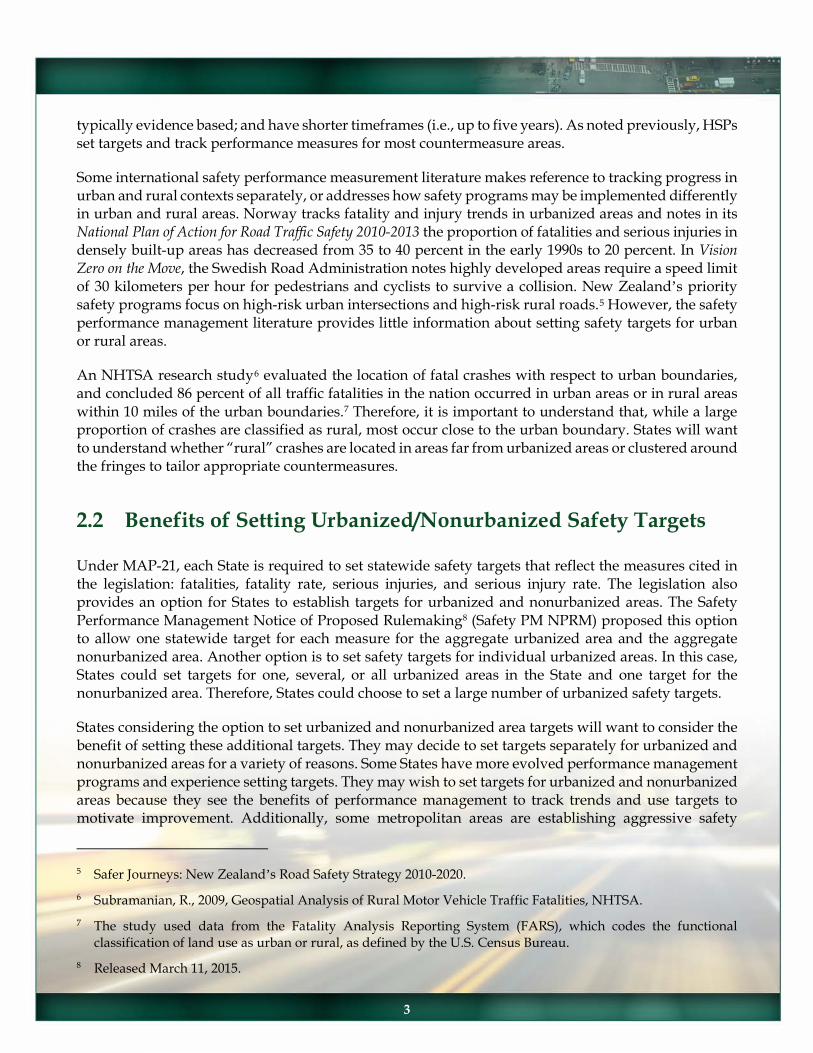
Figure 6-5 Adjusted Urbanized Areas and MPO Areas for Three Utah MPOs .................... 36

Figure 6-6 National Fatalities per 100,000 Population Young Drivers versus Total ................ 37

Figure 6-7 Sample Step 2—Consideration of Exogenous Factors Urbanized Areas ............... 39

Figure 6-8 Sample Step 2—Consideration of Exogenous Factors Nonurbanized Areas ......... 40

Figure 6-9 Urbanized Area Fatalities ........................................................................................... 46

Figure 6-10 Nonurbanized Fatalities ............................................................................................. 47

iii

1.0 Introduction

The Federal transportation legislation, Moving Ahead for Progress in the 21st Century (MAP-21), requires the U.S. Department of Transportation (U.S. DOT) under 23 USC 150 to define a set of safety performance measures and States to set targets that reflect the measures. The measures identified in MAP-21 are serious injuries and fatalities per vehicle mile traveled (VMT) and the number of serious injuries and fatalities. MAP-21 also provides the option in 23 U.S.C. 150 for States to set safety targets for urbanized and nonurbanized areas. The purpose of this document is to provide information to States considering setting urbanized or nonurbanized safety targets. The report includes a review of the state of the practice in setting urbanized and nonurbanized safety targets and identifies methods for state Departments of Transportation (DOT) to consider if they decide to set urbanized or nonurbanized targets.

The Federal Highway Administration’s (FHWA) definition of urbanized areas is those with a population of 50,000 or higher, for which boundaries can be adjusted by States. Further information on geography definitions is included in section 3.

Each State Highway Safety Office (SHSO) established under 23 USC 402 and administered by the National Highway Traffic Safety Administration (NHTSA) develops an annual Highway Safety Plan (HSP) and submits an annual evaluation report to NHTSA. Under MAP-21, HSPs were initially required to report on 14 safety performance measures, as defined in the report entitled Traffic Safety Performance Measures for States and Federal Agencies. Bicyclist fatalities was added as a requirement for fiscal year (FY) 2015 reporting, bringing the total up to 15. States are required to develop annual performance targets for 11 of the measures, and to report annual progress on all 15. The NHTSA document recommends that “States report both rural and urban fatalities/VMT, as well as total fatalities/VMT.”

This report provides information on the state of the practice and potential methodologies for integrating urbanized and nonurbanized safety performance measures and targets into a performance-based safety program.

• Section 2 provides a literature review and describes the potential benefits of setting urbanized andnonurbanized targets;

• Section 3 defines the relevant geography;

• Section 4 provides information on the state of the practice for urbanized and nonurbanized safetytarget setting and an analysis of State fatality and serious injury data for urbanized andnonurbanized areas;

• Section 5 provides a framework for safety target setting;

• Section 6 offers information on safety target setting methods for urbanized and nonurbanized areas;and

• Section 7 summarizes key conclusions.

1

2.0 Background

2.1 Literature Review

Previous work has synthesized the state of the practice in safety target setting by States and regions. For the FHWA’s A Compendium of State and Regional Safety Target Setting Practices,1 the research team catalogued national and international safety targets and methods for setting safety targets.

Establishing road safety performance measures and setting targets are widely advocated practices in other parts of the world, particularly in Europe and Australia. The Organization for Economic Cooperation and Development (OECD) suggests setting targets can improve road safety by encouraging more realistic and efficient road safety programs, communicate the importance of road safety to people who can affect it, give direction to policy-makers, motivate stakeholders to act, and hold road transport system managers accountable. The effectiveness of setting road safety targets has been evaluated in only a few studies; however, the available evidence shows reductions in fatalities and fatality rates are associated with target setting.2

Numerous countries throughout the world (with the majority in Europe) have pursued and achieved safety targets over the years. While limited examples of well-described target setting methodologies are available, current practice involves a combination of top-down long-term goals and bottom-up interim targets of shorter duration. A few agencies are developing interim targets aligned to selected countermeasures, their estimated effectiveness, deployment of vehicle safety technologies, and the extent to which countermeasures are successfully/effectively implemented. Such a process requires defining the country’s level of ambition for road safety, taking into account institutional arrangements, developing methods to measure the effectiveness of strategies needed to improve safety, and identifying available resources. This target setting approach combines an idealistic long-term goal with realistic short-term targets.3

The Safety Target Setting Final Report4 catalogued the state of the practice in safety target setting by reviewing key safety documents and surveying safety practitioners. That work emphasized the importance of clearly defining the terms “goal” and “target.” Goals provide a framework and focus for safety efforts. They may be aspirational, such as “zero fatalities”; or numerical, such as the number calculated to “halve fatalities by 2030.” Most States establish measurable objectives in State Strategic Highway Safety Plans (SHSP), although this is not Federally required. Targets are quantitative;

1 http://safety.fhwa.dot.gov/hsip/tpm/docs/compendium.pdf. 2 FHWA, Safety Target Setting Final Report, 2013. 3 FHWA, Performance Management Practices and Methodologies for Setting a National Safety Performance

Target, 2011. 4 http://safety.fhwa.dot.gov/hsip/tpm/docs/safetyfinalrpt.pdf.

2

typically evidence based; and have shorter timeframes (i.e., up to five years). As noted previously, HSPs set targets and track performance measures for most countermeasure areas.

Some international safety performance measurement literature makes reference to tracking progress in urban and rural contexts separately, or addresses how safety programs may be implemented differently in urban and rural areas. Norway tracks fatality and injury trends in urbanized areas and notes in its National Plan of Action for Road Traffic Safety 2010-2013 the proportion of fatalities and serious injuries in densely built-up areas has decreased from 35 to 40 percent in the early 1990s to 20 percent. In Vision Zero on the Move, the Swedish Road Administration notes highly developed areas require a speed limit of 30 kilometers per hour for pedestrians and cyclists to survive a collision. New Zealand’s priority safety programs focus on high-risk urban intersections and high-risk rural roads.5 However, the safety performance management literature provides little information about setting safety targets for urban or rural areas.

An NHTSA research study6 evaluated the location of fatal crashes with respect to urban boundaries, and concluded 86 percent of all traffic fatalities in the nation occurred in urban areas or in rural areas within 10 miles of the urban boundaries.7 Therefore, it is important to understand that, while a large proportion of crashes are classified as rural, most occur close to the urban boundary. States will want to understand whether “rural” crashes are located in areas far from urbanized areas or clustered around the fringes to tailor appropriate countermeasures.

2.2 Benefits of Setting Urbanized/Nonurbanized Safety Targets

Under MAP-21, each State is required to set statewide safety targets that reflect the measures cited in the legislation: fatalities, fatality rate, serious injuries, and serious injury rate. The legislation also provides an option for States to establish targets for urbanized and nonurbanized areas. The Safety Performance Management Notice of Proposed Rulemaking8 (Safety PM NPRM) proposed this option to allow one statewide target for each measure for the aggregate urbanized area and the aggregate nonurbanized area. Another option is to set safety targets for individual urbanized areas. In this case, States could set targets for one, several, or all urbanized areas in the State and one target for the nonurbanized area. Therefore, States could choose to set a large number of urbanized safety targets.

States considering the option to set urbanized and nonurbanized area targets will want to consider the benefit of setting these additional targets. They may decide to set targets separately for urbanized and nonurbanized areas for a variety of reasons. Some States have more evolved performance management programs and experience setting targets. They may wish to set targets for urbanized and nonurbanized areas because they see the benefits of performance management to track trends and use targets to motivate improvement. Additionally, some metropolitan areas are establishing aggressive safety

5 Safer Journeys: New Zealand’s Roa6 Subramanian, R., 2009, Geospatial 7 The study used data from the Fa

classification of land use as urban or8 Released March 11, 2015.

d Safety Strategy 2010-2020.

Analysis of Rural Motor Vehicle Traffic Fatalities, NHTSA.

tality Analysis Reporting System (FARS), which codes the functional rural, as defined by the U.S. Census Bureau.

3

programs (i.e., New York, Los Angeles, and San Francisco have all established Vision Zero as an overarching goal). Therefore, States might wish to establish targets for the urbanized areas in which these cities are located to support the emphasis on safety in these areas.

States vary significantly in the amount of urbanized and nonurbanized areas, and the proportion of fatalities and serious injuries in the urbanized and nonurbanized areas may vary substantially. The first step when considering setting urbanized and nonurbanized area targets is for States to track safety trends separately for urbanized and nonurbanized areas to understand the safety performance in the different geographies. Agencies can determine if they are achieving safety progress in both urbanized and nonurbanized areas equally or having greater success in one area or the other. Setting urbanized or nonurbanized safety targets also may drive increased focus on how safety programs are developed for and resources allocated to urbanized and nonurbanized areas.

As part of this research effort, a Peer Exchange with representatives from eight State DOTs was conducted in September 2014 to discuss urbanized and nonurbanized safety target setting. Additional benefits for urbanized/nonurbanized safety target setting were identified through those discussions.

1. DOT-established urbanized and/or nonurbanized area targets may increase collaboration withSHSOs, which are encouraged to track progress in urban and rural areas.

2. DOT establishment of urbanized and/or nonurbanized area targets may increase collaboration withmetropolitan planning organizations (MPO) and improve understanding of safety trends inurbanized areas, conducting safety planning in these areas, and coordinating on statewide andindividual urbanized area targets.

3. Long-term consideration of urbanized/nonurbanized area geography would help States trackexpenditure distributions in these areas. The impending Model Inventory of Roadway Elements(MIRE) requirement for fundamental data elements under MAP-21 (23 U.S.C. 148(e)(2)(A)) andother data improvements may help optimize resource distribution.

4. Setting a target for urbanized areas might stimulate more collaboration between MPOs, counties,and local jurisdictions on safety strategies.

5. Agencies might find benefit in using urbanized and nonurbanized area performance measures totrack statewide and emphasis area progress. If States find they are not meeting emphasis area goals,analysis of the emphasis areas by urbanized/nonurbanized areas could help identify where futurefocus is needed and provide a reason for reassessing their safety practices.

6. Examining safety data through an urbanized/nonurbanized area lens could draw attention to theneed for increased outreach with certain safety partners (i.e., counties or local agencies).

4

3.0 Geography Definitions

A clear and consistent definition of the terms “urbanized,” “nonurbanized,” “urban,” and “rural” is needed to conduct target setting for urbanized and nonurbanized areas. This section provides information on a range of designations and describes how areas are defined. The area of interest for target setting is the urbanized area.

3.1 Urban Areas

The U.S. Census Bureau defines and delineates the geographic boundaries for urban areas based on residential population after each decennial Census. Census-defined urban areas are used to summarize and report data collected by most Federal agencies. The Census definition of urban area includes urbanized areas of 50,000 or more population and urban clusters of at least 2,500 and less than 50,000 population.

Beginning with the 2000 decennial Census, the Census Bureau has used a geographic information system (GIS) methodology to identify and construct the boundaries for urban areas based on aggregations of Census Blocks. Each urban area is built outward from a core of Census Blocks that meets an initial population density threshold; new blocks are added until the population density falls below a specified threshold, or until the urban area bumps against an adjacent urban area.

Figure 3-1 shows the 2010 urban area boundary for Columbus, Ohio. As shown, urban area boundaries defined by this process tend to be highly irregular in shape and often containing elongated “fingers” that follow major highways, as well as indentations and “holes” that represent areas with little or no residential population (e.g., urban parkland or industrial areas).

Census defined urban area boundaries may not coincide with the jurisdictional boundaries of incorporated cities or towns, counties, or even States. Parts of a particular urban area (e.g., Washington, D.C. or Philadelphia, Pennsylvania) can exist in two or more States.

5

Figure 3-1 2010 Census Urban Area Boundaries in Columbus Ohio

Source: Census.

3.2 FHWA Adjusted Urbanized Area Boundaries

While the above described urban areas, the focus is on urbanized areas, which is the geography to be used for target setting. FHWA and the Census Bureau differ in defining and describing urban and rural areas. The Census Bureau defines urban areas solely for the purpose of tabulating and presenting Census Bureau statistical data. A number of Federal agency programs uses the Census definitions as the starting point (if not the basis) for implementing and determining eligibility for a variety of funding programs.

6

Federal transportation legislation allows for the outward adjustment of Census Bureau-defined urbanized boundaries as the basis for development of adjusted urbanized area boundaries for transportation planning purposes. By Federal rule, these adjusted urbanized area boundaries must encompass the entire Census-designated urbanized area (and are subject to approval by the Secretary of Transportation (23 USC 101(a) (34) and 49 USC 5302(a) (16)-(17)).9

States may adopt the Census boundaries as is, or adjust them for transportation planning purposes. The FHWA does not require Census urbanized area boundary adjustments. The only official requirement is adjusted boundaries must include the original urbanized area boundary defined by the Census Bureau in its entirety. In other words, any adjustment must expand, not contract, the Census Bureau urbanized area boundary. The adjusted urbanized area boundaries also can include other areas that are “urban” in character, but do not meet the Census Bureau’s population threshold (e.g., high-density industrial or commercial areas, urban parks, etc.). The adjusted boundaries also can be expanded to ensure roads do not alternate between urban and rural designations. This geography is called the “adjusted urbanized area” boundary.

Figure 3-2 shows the 2010 Census defined urbanized area boundary (light green) overlaid on the adjusted urbanized area boundary (brighter green) for Columbus, Ohio. The adjusted urbanized boundary fills in several areas throughout Ohio that are more industrial than residential, and aligns the adjusted boundaries with roads to minimize situations where a road alternates between an urban and rural designation.

As noted previously, the key geography used in this research is the FHWA adjusted urbanized area involving urbanized areas with a population of 50,000 or more. This is the geography proposed in the Safety PM NPRM with respect to urbanized and nonurbanized target setting. This definition is used by FHWA for any Federal reporting of urbanized areas in regulations or statistics, such as for the Urbanized Area Summaries on length and daily vehicle miles of travel (table HM-71) and selected characteristics (table HM-72) documented in the FHWA Highway Statistics Series.10

9 . See section 6.

10 http://www.fhwa.dot.gov/policyinformation/statistics/2012/.

http://www.fhwa.dot.gov/planning/processes/statewide/related/highway_functional_classifications/

7

Figure 3-2 Adjusted Urbanized Area Boundaries in Columbus Ohio

Source: Census, FHWA.

8

Tables 3-1 and 3-2 summarize how Census and FHWA urban and urbanized areas are defined by population range and note FHWA urban area boundaries can be adjusted.

Table 3-1 U.S. Census Bureau Urban Area Types Defined by Population Range Census Bureau Area Definition Population Range

Urban Area 2,500+

Urban Clusters 2,500-49,999

Urbanized Area 50,000+

Source: FHWA Highway Functional Classification Concepts, Criteria and Procedures, 2013.

Table 3-2 FHWA Urban Area Types Defined by Population Range

FHWA Area Definition Population Range Allowed Urban Area

Boundary Adjustments

Urban Area 5,000+ Yes

Small Urban Area (From Clusters) 5,000-49,999 Yes

Urbanized Area 50,000+ Yes

Source: FHWA Highway Functional Classification Concepts, Criteria and Procedures, 2013.

3.3 Other Urban and Rural Definitions

FARS definitions of urban and rural can vary from the urbanized area boundaries used by States. FARS uses the following definition for urban areas:11

An urban area is an area whose boundaries shall be those fixed by responsible State and local officials in cooperation with each other and approved by the FHWA, U.S. DOT. Such boundaries are established in accordance with the provisions of Title 23 of the USC. Urban area boundary information is available from State highway or transportation departments. In the event that boundaries have not been fixed as above for any urban place designated by the Bureau of the Census having a population of 5,000 or more, the area within boundaries fixed by the Bureau of the Census shall be an urban area.

NHTSA produces annual fact sheets on urban and rural crashes using the urban and rural definitions that FARS analysts report from each State. However, as FARS data are geocoded, the number of fatalities falling within the urbanized area boundary can be calculated using GIS. For consistency, beginning in 2016, NHTSA will begin reporting data using the FHWA adjusted urbanized areas geography.

Most States also use other definitions for urban and rural. Common definitions include considering crashes occurring inside the boundaries of a municipality “urban”, or defining urban areas as those over a certain population threshold. The urban/rural definitions used for crash reporting forms are likely different from Federal definitions, so that is not a reliable source for these computations.

11 FARS Users Manual 1975-2012.

9

4.0 State of the Practice

In this section, because States currently do not necessarily track safety data by urbanized and nonurbanized area geographies, the terms urban and rural are used. Review of the most recent SHSPs, HSPs (FY 2014), and HSIP Annual Reports (FY 2013) in all 50 States revealed only one State (Georgia) set urban or rural targets in its SHSP (figure 4-1, left). A number of States include urban and rural fatality, serious injury, or crash data in their SHSPs to track overall trends (figure 4-1, right). Of those, some track the number of crashes within an SHSP emphasis area that are urban or rural.

Figure 4-1 Existence of Urban and Rural Targets and Crash Data Analysis in SHSPs

421 1

11

320

5

10

15

20

25

30

35

40

Urban / Rural Fatalities Urban / Rural Serious Injuries Urban / Rural Fatalities Urban / Rural Serious Injuries

Targets Data

Other (e.g. Crashes) Rate Number Number and Rate

Source: Cambridge Systematics, Inc.

States more commonly include safety targets for urban and rural areas in HSPs than in other State safety documents. This can be attributed to the 2008 Traffic Safety Performance Measures for States and Federal Agencies document which notes, “States should report both rural and urban fatalities/VMT as well as total fatalities/VMT.” More than one-half of HSPs include urban fatality targets (figure 4-2, left), but only one includes an urban serious injury target. Nearly all HSPs track rates and/or numbers of urban and rural fatalities, but only a few States include urban and rural serious injury data (figure 4-2, right).

45

50

10

Figure 4-2 Existence of Urban and Rural Targets and Crash Data Analysis in HSPs

Source: Cambridge Systematics, Inc.

As there is no current requirement, no States report urban or rural safety targets in Highway Safety Improvement Plan (HSIP) Annual Reports. Some HSIP annual reports include data on urban and rural crashes, as shown in figure 4-3. Moving forward, it is expected States will begin to report safety targets in these documents, as proposed in the Safety PM NPRM.

1

28

1 20

5

10

15

20

25

30

35

Urban / Rural Fatalities

13 4

23

2 2

17

Urban / Rural Serious Injuries Urban / Rural Fatalities Urban / Rural Serious Injuries

Targets DataOther (e.g. Crashes) Rate Number Number and Rate

40

45

50

11

Figure 4-3 Existence of Urban and Rural Crash Data Analysis in HSIP Annual Reports

5

13

1

0

5

10

15

20

Number only Rate only Number and Rate Other (e.g. Crashes)

Urban / Rural Fatalities Urban / Rural Serious Injuries

Source: Cambridge Systematics, Inc.

The research team analyzed FARS data using GIS to calculate the proportion of fatalities in urbanized and nonurbanized areas according to the FHWA adjusted urbanized area geography using the most recent boundary data available for all States (2000). Table 4-1 summarizes the annual average number and percent of statewide fatalities located in urbanized and nonurbanized areas over a five-year period (2007 to 2011). In those cases where the sum of urbanized and nonurbanized area fatalities is less than the total, some fatalities were not able to be geolocated (e.g., location data were incorrect or missing), and these are indicated in table 4-1 as “annual average nonlocatable fatalities”. As noted previously, the FHWA adjusted urbanized area12 boundary includes only areas with population more than 50,000. There is wide variation across States in the percentage of fatalities that occur in urbanized areas, ranging from 6 percent for North Dakota to 84 percent in Massachusetts, which is a reflection of the extent to which the land area is urbanized in a State. On a national level, 41 percent of fatalities occur in urbanized areas and 59 percent in nonurbanized areas. The percentages of urbanized and nonurbanized area fatalities in table 4-1 are calculated after removing nonlocatable fatalities.

12 When the term FHWA adjusted urban boundary is used in other contexts, this includes areas with population above 5,000.

20 20

25

12

Table 4-1 Annual Average Fatalities in Urbanized and Nonurbanized Areas

2007 to 2011

State

Total Annual Average Fatalities

Annual Average

Nonlocatable Fatalities

FHWA 2000 Urbanized

Area Fatalities

Percent Urbanized

Area Fatalities

FHWA 2000 Nonurbanized Area Fatalities

Percent Nonurbanized

Fatalities

Alabama 936 1 292 31% 643 69%

Alaska 67 0 20 29% 47 70%

Arizona 870 35 382 44% 453 56%

Arkansas 593 1 107 18% 485 82%

California 3,206 2 1,929 60% 1,275 40%

Colorado 493 0 196 40% 297 60%

Connecticut 272 4 203 74% 65 25%

Delaware 111 0 45 40% 66 60%

Florida 2,719 76 1,724 64% 919 37%

Georgia 1,355 59 501 37% 795 63%

Hawaii 113 4 40 36% 69 64%

Idaho 217 0 28 13% 190 87%

Illinois 1,009 0 517 51% 493 49%

Indiana 779 11 244 31% 524 69%

Iowa 396 1 70 18% 325 82%

Kansas 401 1 81 20% 319 80%

Kentucky 792 1 139 18% 652 82%

Louisiana 826 2 268 32% 556 68%

Maine 159 1 20 13% 138 87%

Maryland 546 5 330 60% 211 40%

Massachusetts 364 9 307 84% 48 16%

Michigan 954 0 435 46% 519 54%

Minnesota 433 0 111 26% 322 74%

Mississippi 727 0 96 13% 631 87%

Missouri 887 1 262 30% 624 70%

Montana 225 0 19 9% 206 91%

Nebraska 212 0 31 15% 181 85%

Nevada 289 1 160 55% 128 44%

New Hampshire 119 0 34 28% 85 72%

New Jersey 616 7 453 74% 156 26%

New Mexico 368 0 77 21% 292 79%

13

State

Total Annual Average Fatalities

Annual Average

Nonlocatable Fatalities

FHWA 2000 Urbanized

Area Fatalities

Percent Urbanized

Area Fatalities

FHWA 2000 Nonurbanized Area Fatalities

Percent Nonurbanized

Fatalities

New York 1,199 110 727 61% 362 39%

North Carolina 1,381 75 394 29% 912 71%

North Dakota 122 1 7 6% 114 94%

Ohio 1,113 1 465 42% 647 58%

Oklahoma 723 14 155 21% 554 79%

Oregon 379 1 86 23% 292 77%

Pennsylvania 1,365 3 552 41% 810 60%

Rhode Island 70 0 55 79% 15 21%

South Carolina 906 1 240 27% 665 73%

South Dakota 130 0 9 7% 121 93%

Tennessee 1,044 1 364 35% 679 65%

Texas 3,215 46 1,378 43% 1791 57%

Utah 262 0 115 44% 147 56%

Vermont 68 1 6 10% 61 91%

Virginia 823 46 304 37% 473 63%

Washington 499 3 206 41% 290 59%

West Virginia 364 1 54 15% 309 85%

Wisconsin 615 0 150 24% 466 76%

Wyoming 146 1 12 9% 133 91%

Total 35,476 2 14,402 41% 21,074 59%

Source: Cambridge Systematics, Inc.

To calculate fatality rates for adjusted urbanized areas, it was necessary to obtain VMT data from FHWA. Currently, VMT data are provided for urbanized areas on the FHWA Highway Statistics web site, but data are provided in the aggregate for urbanized areas spanning multiple States. Therefore, FHWA provided calculations for urbanized area VMT by State for use in this report. Each State must calculate VMT for its annual submission to the Highway Performance Monitoring System (HPMS) maintained by FHWA and should be in possession of its urbanized area VMT.

Table 4-2 shows average annual fatality rates using 2007 to 2011 FARS data and 2009 to 2011 VMT data. Ideally, a five-year average of VMT data would be used with five-year average fatalities, but for this study only select years of urbanized area VMT data by State were available. In every State, the nonurbanized fatality rate was higher than the urbanized fatality rate and statewide fatality rate. Statewide fatality rates range from 0.70 in Massachusetts to 2.03 in Montana. Urbanized area fatality rates are between 0.42 for Minnesota and 1.49 in Nevada, and nonurbanized fatality rates range from 1.08 in Minnesota to 2.95 in Nevada.

14

Table 4-2 FHWA 2000 Adjusted Urbanized Area Fatality Rates

State Statewide

Fatality Rate Urbanized Area

Fatality Rate Nonurbanized Area

Fatality Rate

Alabama 1.48 1.15 1.69

Alaska 1.46 1.22 1.59

Arizona 1.45 1.00 2.27

Arkansas 1.79 0.98 2.18

California 1.01 0.78 1.83

Colorado 1.06 0.70 1.61

Connecticut 0.89 0.79 1.41

Delaware 1.28 0.90 1.79

Florida 1.40 1.14 2.31

Georgia 1.30 0.83 1.93

Hawaii 1.20 0.80 1.65

Idaho 1.41 0.54 1.84

Illinois 0.99 0.74 1.56

Indiana 1.08 0.65 1.54

Iowa 1.29 0.77 1.51

Kansas 1.34 0.67 1.80

Kentucky 1.68 0.93 2.04

Louisiana 1.83 1.25 2.35

Maine 1.12 0.69 1.23

Maryland 1.00 0.84 1.37

Massachusetts 0.70 0.65 1.12

Michigan 1.01 0.76 1.42

Minnesota 0.77 0.42 1.08

Mississippi 1.88 0.98 2.19

Missouri 1.33 0.81 1.81

Montana 2.03 1.30 2.14

Nebraska 1.12 0.49 1.43

Nevada 1.91 1.49 2.95

New Hampshire 0.92 0.61 1.16

New Jersey 0.88 0.73 2.17

New Mexico 1.47 1.01 1.67

New York 0.95 0.83 1.24

North Carolina 1.34 0.76 1.92

15

State Statewide

Fatality Rate Urbanized Area

Fatality Rate Nonurbanized Area

Fatality Rate

North Dakota 1.45 0.47 1.68

Ohio 1.00 0.69 1.46

Oklahoma 1.53 0.79 2.05

Oregon 1.15 0.58 1.61

Pennsylvania 1.39 0.99 1.89

Rhode Island 0.87 0.79 1.39

South Carolina 1.87 1.18 2.38

South Dakota 1.46 0.53 1.67

Tennessee 1.53 1.07 1.99

Texas 1.41 0.94 2.27

Utah 1.05 0.72 1.62

Vermont 1.26 0.82 1.34

Virginia 1.03 0.64 1.60

Washington 0.90 0.56 1.54

West Virginia 1.91 1.00 2.27

Wisconsin 1.06 0.63 1.37

Wyoming 1.58 1.19 1.63

Total 1.23 0.84 1.80

Source: Fatality rate based on annual average 2007 to 2011 FARS and 2009 to 2011 VMT provided by FHWA.

As shown in table 4-2, the nonurbanized fatality rate nationally is 1.8, and the urbanized area fatality rate is 0.84.

When comparing two States using fatality rates, one State may appear to be safer than another based on a comparison of their statewide fatality rates; however, the other State could look safer based on a comparison of urbanized fatality rates. Simpson’s Paradox represents the statistical phenomenon of stratifying aggregate data into two or more groups, and finding that analysis of the smaller groups results in opposing conclusions. It illustrates how the safety profile of a State is affected by the proportion of urbanized and nonurbanized VMT in the calculation.

Table 4-3 shows California has a lower statewide fatality rate than South Dakota; therefore, California roads appear safer. However, the fatality rates for urbanized and nonurbanized areas are both lower in South Dakota than in California.

16

Table 4-3 Simpson’s Paradox Illustration

State Percent Urbanized

Area VMT

Percent Nonurbanized

Area VMT Statewide Fatality

Rate Urbanized Area

Fatality Rate Nonurbanized

Area Fatality Rate

California 78% 22% 1.01 0.78 1.83

South Dakota 19% 81% 1.46 0.53 1.67

Source: Fatality rate based on annual average 2007 to 2011 FARS and 2009 VMT provided by FHWA.

A national dataset does not exist with comprehensive, high quality injury crash data like the FARS database for fatal crashes. To conduct GIS analysis of crash locations and determine the proportion of urbanized and nonurbanized serious injury crashes, locations of all serious injury crashes on all public roads are needed for at least one if not multiple five-year periods. To analyze the proportion of urbanized versus nonurbanized serious injuries, the study team collected data on serious injuries maintained in State crash records systems from all 50 States.

The study team ultimately obtained usable data for 20 States, which is presented in table 4-4. Usable data was defined as data for which crashes on all public roads were geolocated, and for which data on serious injuries was clearly identified separately from other levels of injury severity. For each State, five years of data were used, but not all time periods were consistent, as noted in the columns to the right. The percentage of serious injuries in urbanized areas is higher than for fatalities. Crashes in urbanized areas differ from those in nonurbanized areas (e.g., there are more bicycle, pedestrian, and intersection crashes in urbanized areas). To calculate the proportion of serious injuries in urbanized versus nonurbanized areas, the 2000 map of adjusted urbanized areas was used, which was the last year for which GIS data were available for all States.

17

Table 4-4 Serious Injury Numbers for Select States

State Percent of Urbanized

Percent of Nonurbanized

Number of Serious

Injuries

Number of Urbanized

Serious Injuries

Number of Nonurbanized

Serious Injuries

Start Year

End Year

Alaska 51.6% 48.4% 435 225 211 2006 2010

Arizona 67.1% 32.9% 5,020 3,367 1,652 2008 2012

Colorado 49.2% 50.8% 4,128 2,033 2,096 2008 2012

Iowa 30.7% 69.3% 1,694 520 1,175 2008 2012

Illinois 66.5% 33.5% 9,704 6,456 3,248 2008 2012

Louisiana 43.2% 56.8% 1,424 616 808 2008 2012

Maine 27.7% 72.3% 636 176 460 2008 2012

Michigan 50.6% 49.4% 6,116 3,093 3,022 2008 2012

Minnesota 22.3% 77.7% 1,268 283 984 2008 2012

Missouri 39.3% 60.7% 6,143 2,416 3,727 2008 2012

Montana 13.4% 86.6% 1,094 147 947 2008 2012

Nebraska 33.8% 66.2% 1,721 582 1,139 2007 2011

New Jersey 64.1% 35.9% 1,532 982 550 2008 2012

New York 68.9% 31.1% 12,932 8,912 4,019 2008 2012

Ohio 52.1% 47.9% 9,720 5,061 4,659 2008 2012

Oklahoma 39.4% 60.6% 3,663 1,445 2,218 2008 2012

Oregon 43.3% 56.7% 1,537 666 871 2008 2012

Pennsylvania 46.5% 53.5% 2,871 1,335 1,537 2008 2012

South Dakota 21.7% 78.3% 837 182 655 2008 2012

Texas 50.7% 49.3% 15,459 7,839 7,621 2009 2013

Source: Cambridge Systematics, Inc., and State crash databases.

Table 4-5 presents serious injury rates, which are significantly higher than fatality rates, given the numbers of serious injury crashes are higher than fatal crashes. The table presents annual average data for a five-year period, but not all time periods are consistent, as noted by the columns indicating the years included in the analysis.

18

Table 4-5 Serious Injury Rates for Selected States

State

Annual Average Number of

Serious Injuries

Statewide Serious Injury Rate

(per 100 MVMT)

Urbanized Area Serious Injury

Rate (per 100 MVMT

Nonurbanized Serious Injury

Rate Start Year

End Year

Alaska 435 9.4 13.7 7.1 2006 2010

Arizona 5,020 8.4 8.8 7.7 2008 2012

Colorado 4,128 8.9 7.2 11.4 2008 2012

Iowa 1,694 5.5 5.7 5.5 2008 2012

Illinois 9,704 9.5 9.2 10.3 2008 2012

Louisiana 1,424 3.2 2.9 3.4 2008 2012

Maine 636 4.5 6.1 4.1 2008 2012

Michigan 6,116 6.5 5.4 8.3 2008 2012

Minnesota 1,268 2.3 1.1 3.3 2008 2012

Missouri 6,143 9.2 7.4 10.8 2008 2012

Montana 1,094 9.9 10.0 9.8 2008 2012

Nebraska 1,721 9.1 9.2 9.0 2007 2011

New Jersey 1,532 2.2 1.6 7.3 2008 2012

New York 12,932 10.3 10.1 10.6 2008 2012

Ohio 9,720 8.7 7.5 10.5 2008 2012

Oklahoma 3,663 7.7 7.3 8.0 2008 2012

Oregon 1,537 4.7 4.5 4.8 2008 2012

Pennsylvania 2,871 2.9 2.4 3.6 2008 2012

South Dakota 837 9.4 10.8 9.1 2008 2012

Texas 15,459 6.8 5.3 9.4 2009 2013

Source: Cambridge Systematics, Inc., State crash databases, VMT data for 2009 to 2011 provided by FHWA.

19

5.0 Safety Target Setting Framework

5.1 What is Evidence-Based Target Setting?

MAP-21’s performance management orientation has increased attention to performance measures and target setting. The policy in USC 23 (150) states:

Performance management will transform the Federal-aid highway program and provide a means to the most efficient investment of Federal transportation funds by refocusing on national transportation goals, increasing the accountability and transparency of the Federal-aid highway program, and improving project decision-making through performance-based planning and programming.

The Safety PM NPRM provided an indication of potential Federal guidance on target setting implementation and presented the option for urbanized and nonurbanized area target setting. As with any management framework, understanding the semantics of the elements of the framework is important to effectively implement the approach. This section presents an approach to evidence-based target setting. The NHTSA Interim Final Rule calls for evidence-based target setting. It states:13

“State HSPs must now provide for performance measures and targets that are evidence-based…. The State process for setting targets in the HSP must be based on an analysis of data trends and a resource allocation assessment.”

There are two basic ways to think about target setting, one of which is evidence based:

• Aspirational or vision-based targets. Sometimes, agencies will use “target” to refer to a long-term vision for future performance—the ultimate goal. Many transportation agencies are setting vision-based targets for zero fatalities (i.e., Vision Zero, Toward Zero Deaths); and interim targets for progress towards this vision (i.e., reduce fatalities by one-half within 20 years).

• Evidence or investment-based targets. Evidence-based target setting is a narrower approach to target setting—focused specifically on what can be achieved within the context of a set of investments, policies, and strategies defined within a shorter timeframe when future trends can be forecasted with more accuracy based on available data.

In the context of MAP-21, HSIP14 annual reports will have to include targets and explain how fatalities and serious injuries will be reduced. This is evidence-based target setting, examining how a specific set of actions contributes to improved performance over a specific time horizon. In addition, when a performance measure, such as the number of urbanized area fatalities, is used by multiple agencies (e.g., State DOT and SHSO), the targets will need to be aligned.

13 http://www.gpo.gov/fdsys/pkg/FR-2013-01-23/html/2013-00682.htm. 14 The HSIP is the safety program through which infrastructure-oriented safety projects are prioritized and

programmed. The projects identified in the HSIP also are included in the State Transportation Improvement Program (STIP).

20

While these two approaches are distinct, they are not necessarily in conflict. A zero-based vision or target is useful for galvanizing support around a planning effort, and for ensuring successful strategies are considered and/or implemented while keeping the focus on a clear long-term goal.

Evidence-based targets, in contrast, promote accountability and encourage agencies to consider the tradeoffs of their investments across different program areas. Being able to demonstrate the benefits of different levels of investment in safety (and other programs) helps decision-makers better understand the implications of investment in various program areas. Target setting with this approach is derived from considering the tradeoffs among investment levels.

5.2 How to Conduct Evidence-Based Target Setting

The basic concept for evidence-based target setting is to link investments and policy decisions to performance. Typically, this is done by reviewing the achievements resulting from previous investments and applying that knowledge to estimate the expected improvement in safety outcomes likely to be achieved given varying levels of investment in the future.

As agencies begin setting evidence-based targets, the approaches outlined below should be considered. The steps for using countermeasure data in target setting are relatively simple, although implementation may be complex:

1. Use trend analysis.

2. Consider exogenous factors (i.e., population, distribution between urbanized and nonurbanized areas, anticipated policies).

3. Forecast fatality reductions based on planned implementation of proven countermeasures:

a. Identify potential for application of countermeasures (through SHSP, HSP, HSIP, or other planning processes);

b. Identify data on expected countermeasure or legislation impact;

c. Develop constrained list of countermeasures based on expected effectiveness and available resources (i.e., expected lives saved per dollar of investment); and

d. Estimate system, region, or State benefits based on the aggregation of expected countermeasures, discounting for potential overlap among emphasis areas.

Once the trend line forecast is developed, consideration of exogenous factors and forecasted fatality reductions will help quantitatively estimate how aggressive the target can be. Agencies may wish to include countermeasures not previously implemented. For those projects or programs without known effectiveness data, evaluation should be included as a component of the project. Figure 5-1 shows how these steps can be used to develop an evidence-based fatality target and what questions are being answered at each phase.

21

Figure 5-1 Target Setting Steps

Where are we now?

Estimate existing trend

What external factors will impact our target?

Adjust trend for expected external/exogenous factors

What is the impact of improvements?

Estimate target based on forecasted fatality reduction

from safety plans

Safe

ty M

easu

re

Time

1 2 3

Scenario 3

Time

Scenario 1

Safe

ty M

easu

re

Safe

ty M

easu

re

Time

Scenario 2

Source: Cambridge Systematics, Inc.

The appropriate combination of the steps described above will depend on the factors and issues in each State or region. While these steps are quite general, they point to a direction agencies can pursue, and some illustrative examples are provided in this report. In the short term, agencies will have to consider multiple pieces of information to set a meaningful, evidence-based target. Safety analysis tools currently available are described below, as well as an overview of each of the analytical approaches. Details on data and methodologies are provided in section 6.

Using Trend Analysis

Examining fatality trends is a simple approach. It is generally the first step States take in understanding safety performance and potential future safety gains. Given the potential variation in crashes and severity each year, it is common for States to look at a rolling average of multiple years, as well as single-year results. American Association of State Highway and Transportation Officials’ (AASHTO) Standing Committee on Performance Management (SCOPM) recommends in its SCOPM Task Force Findings on MAP-21 Performance Measure Target-Setting15 that States use five-year moving averages to evaluate trends.

15 SCOPM Task Force Findings on MAP-21 Performance Measure Target-Setting, http://scopm.transportation.org/Documents/SCOPM%20Task%20Force%20Findings%20on%20Performance%20Measure%20Target-Setting%20FINAL%20v2%20(3-25-2013).pdf, page 13.

22

Figure 5-2 is a graphical example of trend analysis showing both a multiyear average and individual year data. As shown, multiyear averages smooth the variation in the data year to year. More detail on calculating trends and projections is provided in section 6.9 on Projection Methods.

Figure 5-2 Pennsylvania Roadway Fatality Trend

Source: Pennsylvania Highway Safety Plan, Cambridge Systematics, Inc.

Consideration of Exogenous Factors

Agencies will likely want to consider the impact of exogenous factors, those which are outside the safety field but affect safety, in defining their targets. Because demographic and technological factors play a significant role in safety, it is important to consider how these trends impact target setting.

Technology is likely to play a major role in helping the U.S. and other nations reduce fatalities, serious injuries, and crashes. Recently, in-vehicle technology, such as curtain airbags or rearview cameras, has been one of the largest contributors to improved roadway safety. New technologies, such as vehicles that “read the road” (e.g., can identify lane markings and help reduce lane departure) and self-driving vehicles, will have major safety implications. Because many of these technologies are immature, the task in the short term is to determine how much can be achieved with currently available technologies and other nontechnology-oriented strategies.

0

200

400

600

800

1,000

1,200

1,400

1,600

1,800

2007 2008

Total Fatalities

23

5-Year Average Fatalities

2005 2006 2009 2010 2011 2012 2013 2014

Demographics are one factor explaining variation in fatalities. Population is increasingly shifting into urban areas. The nation’s urban population increased by 12.1 percent from 2000 to 2010, outpacing the nation’s overall growth rate of 9.7 percent for the same period, according to the U.S. Census Bureau.16

Another consideration is how involvement in fatal crashes varies greatly based on age and gender. For example, the crash rate for drivers age 16 to 19 is 4.6 crashes per 100 million VMT (100 MVMT), compared to 1.2 crashes per 100 MVMT for ages 30 to 69.17 Within these age groups, crash rates are higher for males than females. Taking into account forecasted demographic trends can help States develop better targets.

It is often useful to leverage the experience of other States when evaluating the impact of exogenous factors. States or regions that have undergone similar transitions can provide helpful insights about expected safety impacts.

Impact of Legislative Changes

Implementation of key safety legislation can have a significant impact on traffic safety. As shown in figure 5-3, at a national level, legislative changes resulting from Federal transportation bills are correlated with reductions in the number of fatalities and the fatality rate.

Evidence at the State level suggests enacting legislation, such as primary seatbelt laws, motorcycle helmet laws, and strengthened graduated driver licensing (GDL) requirements, reduces fatalities.18 However, the degree of fatality reduction is tied to the level of resources applied to implementation and enforcement. Information about calculating performance of planned improvements is provided in section 6.7.

16 https://www.census.gov/newsroom/releases/archives/2010_census/cb12-50.html. 17 http://www.iihs.org/iihs/topics/t/teenagers/fatalityfacts/teenagers. 18 Countermeasures that Work, 2013, NHTSA.

24

Figure 5-3 National Legislative History and Fatality Trends

ISTEA—Intermodal Surface Transportation Efficiency Act of 1991; TEA-21—Transportation Equity Act for the 21st Century; and SAFETEA-LU—Safe, Accountable, Flexible, Efficient Transportation Equity Act: A Legacy for Users.

Source: Cambridge Systematics, Inc.

25

Forecasting Reductions Based on Planned Implementation of Proven Countermeasures

Agencies can use performance analysis to understand what is likely to be achieved by a planned safety program, which can then inform the evidence-based target setting process. This approach builds on existing efforts by State DOTs to understand effectiveness of countermeasures implemented in their State. State DOTs, FHWA, and other national research organizations examine countermeasure effectiveness on an ongoing basis.

Particularly for infrastructure improvements, forecasts of safety impacts resulting from implementation of proven countermeasures can be made using crash modification factors (CMF). Agencies can draw upon nationally developed CMFs, such as those provided in the Highway Safety Manual (HSM) or the CMF Clearinghouse, as well as the knowledge they already have about the effectiveness of projects implemented in their State or region. Results from implemented projects that address the unique conditions of the State or region are likely the most useful. A target is evidence based if it incorporates the expected results of a set of improvements in a plan.

Traditional benefit-cost analysis estimates the value of potential crash reduction based on CMFs for a given treatment. States can also look at the impact of a broader set of investments on fatalities by comparing historical investment trends against the associated impact on targeted crashes to determine what types of investments are most effective in reducing fatalities. This will help provide a sense of the level of investment required to reduce fatalities in one emphasis area compared to another.

Under MAP-21, States are required to report to the U.S. DOT Secretary on progress made implementing highway safety improvements, the effectiveness of those improvements, and the extent to which fatalities and serious injuries on all public roads have been reduced, including a breakdown by functional classification and ownership to the maximum extent practicable.19 As part of this reporting process, States have to describe the effectiveness of HSIP-funded projects. States also should determine the benefits and costs of not only infrastructure programs, but also behavioral, enforcement, Emergency Medical Services (EMS), and other programs. This type of evaluation should be incorporated into as many projects as possible for which good effectiveness data do not yet exist to develop new CMFs.

Behavioral programs are impacted by the manner of implementation, and a State’s culture and effectiveness data are less likely to be available; therefore, it is even more beneficial for States to study program effectiveness on behavioral countermeasures. This will enable States to know which programs are delivering results and are most cost-effective. Moving forward, this State-specific safety effectiveness information will help determine which programs to replicate and expand, and which to modify or discontinue. The results can be used to forecast the outcomes of a safety plan and support the target setting process. For example, on average, States that pass primary seat belt laws can expect to increase seat belt use by eight-percentage points. Depending on the level of high-visibility enforcement that they employ, however, far greater results are possible. One study found that

19 http://www.fhwa.dot.gov/map21/factsheets/hsip.cfm.

26

passenger vehicle driver death rates dropped by seven percent when States changed from secondary to primary enforcement.20

Safety Analysis Tools

In recent years, a number of safety analysis tools have become available that can aid in forecasting fatality and injury reductions associated with countermeasures. Estimating the impact of safety projects supports the development and refinement of evidence-based safety targets. Tools include the following:

• Highway Safety Manual (HSM) provides practitioners with information and tools to consider safety when making decisions related to design and operation of roadways. The HSM assists practitioners in selecting countermeasures and prioritizing projects, comparing alternatives, and quantifying and predicting the safety performance of roadway elements considered in planning, design, construction, maintenance, and operation.

• Interactive Highway Safety Design Model (IHSDM) is a suite of software analysis tools for evaluating safety and operational effects of geometric design decisions on highways. IHSDM is a decision support tool that provides estimates of existing or proposed highway designs’ expected safety and operational performance, and checks designs against relevant design policy values.

• SafetyAnalyst provides a set of software tools used by State and local highway agencies for highway safety management. It incorporates state-of-the-art safety management approaches into computerized analytical tools for guiding the decision-making process to identify safety improvement needs and develop a systemwide program of site-specific improvement projects.

• HSIP Manual provides an overview of the HSIP and presents State and local agencies with tools and resources to implement the HSIP. The manual provides information related to planning, implementation, and evaluation of State and local HSIPs and projects.

• CMF Clearinghouse provides a regularly updated on-line repository of CMFs, which are used to forecast the impact of a countermeasure on crash frequency and severity. The Clearinghouse also provides a mechanism for sharing newly developed CMFs and educational information on the proper application of CMFs.

• Countermeasures That Work is a resource, updated annually by NHTSA, which documents the effectiveness of safety countermeasures for noninfrastructure-oriented major highway safety problem areas (e.g., behaviors, population groups, and vulnerable user types). Calculating effectiveness of noninfrastructure strategies is more challenging than that for infrastructure-oriented approaches. Nevertheless, this resource provides evidence-based information that can inform project result forecasts and safety target setting.

20 NHTSA, Countermeasures that Work: A Highway Safety Countermeasure Guide for State Highway Safety Offices, Seventh Edition, 2013.

27

6.0 Data and Methods for Evidence-Based Urbanized and Nonurbanized Targets

Safety analysis is a data-driven process. For performance measures to be useful, relevant data must exist. Realistic targets also require the existence of appropriate data. This section outlines the core data needed for fatality and serious injury target setting and identifies other data useful for further refining safety targets. The information is grouped into three categories: 1) trend data; 2) data on exogenous factors; and 3) countermeasure impact data.

The following sections walk through the technical analysis aspects of methods and data requirements for setting urbanized and nonurbanized safety targets.

6.1 Step 1. Identifying Trends

Fatality and Serious Injury Data

A core data element States must collect for trend analysis is fatalities. Fatal crash data are high quality as they are standardized among States and available in the national FARS database. Each State has one or more FARS analysts who review crash reports and correct errors. All fatal crashes include detailed location data and can be mapped in GIS, which is necessary to enable analysis of data and target setting for urbanized or nonurbanized areas. FARS contains comprehensive information on factors involved in each crash, which enables understanding the distribution of crash types between urbanized and nonurbanized areas. Therefore, analyzing trends for fatalities and fatality rates by urbanized versus nonurbanized areas is feasible for all States. It is useful to observe actual annual data trends, as well as five-year moving average trends, as will be required for Federal safety performance monitoring.

Where are we now?

Estimate existing trend

Safe

ty M

easu

re

Time

1

Source: Cambridge Systematics, Inc.

Serious injury data is less straightforward. The primary challenge for setting serious injury targets is the quality of injury data, which are maintained individually by States in their own crash databases. The quality of injury data varies greatly. Key aspects of injury data that affect the ability to set urbanized and nonurbanized area targets are crash location, injury severity, years of data available, and data completeness, which are described in more detail below.

Crash Location Information

To categorize crashes as urbanized or nonurbanized, accurate information on crash location is needed. Ideally, datasets include latitude and longitude coordinates so the exact point location of a crash can be identified. Many States use Geographic Positioning System (GPS) data as part of the crash reporting process, so latitude and longitude are part of each crash record. With point location data such as these, crashes can easily be mapped in GIS and determined to be inside or outside the FHWA-adjusted urbanized area boundary. One concern related to the use of GPS coordinate data is that the law enforcement officer must take the GPS reading at the exact crash location, which is not always possible. Map-based location methods are becoming increasingly common, which should improve the accuracy

28

of crash location data. With this approach, the law enforcement officer locates the crash on an electronic map, clicks on the map, and coordinates and other location information are automatically entered into the crash record.

Another approach to location of crashes is the use of a State’s linear referencing system (LRS). Linear referencing is used by many State DOTs to associate features (e.g., signs, guardrail, etc.) or events with the roadway network. The LRS is associated with the State’s roadway infrastructure file, so crashes can be located with respect to mileposts or other roadway location information. This approach to locating crashes is generally quite good, although location information may have a margin of error. For example, if a State has mileposts only every mile, a responder to the crash scene will note the closest milepost on the crash report, but the actual crash location could be some distance of less than a mile away from that milepost. Most States are working toward development of a high-quality LRS, but some currently do not have a fully functional system in operation.

A number of States have location data only for crashes on the State highway system and are missing this information on nonstate-owned facilities. This is frequently the case because State law enforcement agencies usually have the ability to input crash reports electronically in their vehicles, possibly with the assistance of GPS for crash locations, but local law enforcement agencies may not.

In the absence of precise location data described above, some location data for serious injury crashes may be available, such as an address, zip code, or the jurisdiction in which a crash occurred (e.g., city name). These data can be useful in determining whether injuries have occurred within or outside the FHWA-adjusted urbanized area, especially if entire zones (i.e., city or zip code) are known to be contained within a boundary. Some assumptions would need to be made, however, in the event the FHWA urbanized area boundary bisects one or more zones.

Injury Severity

A second facet of working with data to calculate serious injury numbers or rates is knowing the severity of injury crashes. To calculate a serious injury number or rate, it is necessary to separate severe injury crashes from other injury crashes.

The Safety PM NPRM proposes to define serious injuries in a manner that would provide for a uniform definition for national reporting in this performance area. The NPRM proposes States adopt the latest edition Model Minimum Uniform Crash Criteria (MMUCC) definition and attribute for ‘‘Suspected Serious Injury (A).’’

The MMUCC is a voluntary and collaborative effort to generate uniform, accurate, reliable, and credible crash data for data-driven highway safety decisions within a State, between States, and at the national level. These guidelines suggest a manner for classifying all data associated with a crash in a State’s crash database, including injury severity. Each State, however, maintains its own crash form and only periodically updates the crash form because doing so requires financial and staff resources, and makes it difficult to compare data across years. Over time, States are modifying crash data and increasingly following the MMUCC; however, significant variation still occurs among terms used in each State. The NPRM proposes a requirement to use the latest version of the MMUCC (currently Version 4), which means some States need to change crash report forms. Injury severity classification often varies by State; States may use the KABCO scale shown in table 6-1, or record injury severity using other categories. Category A below is the code used for calculating numbers or rates of suspected serious injuries.

29

Table 6-1 KABCO Injury Classification Classification Definition

O Property Damage Only

C Possible Injury

B Suspected Minor Injury

A Suspected Serious Injury

K Fatal Injury

U Unknown

Source: MMUCC, Version 4.

To calculate the number of serious injuries or a serious injury rate, the data required is the number of people experiencing injuries. In some cases, crash databases are oriented around the crash and do not reliably report the number of persons injured and the level of injury severity sustained by each person. For the purpose of developing a serious injury target, it must be possible to isolate only those people sustaining serious injuries and information about those crashes. In the event information is available only for the crash severity, but not for the number of injuries or severity of injuries, it is possible to make assumptions about the number of severe injuries resulting from each crash type, but this will not be as accurate as if the data were reported directly. States could use the information on the probability that a crash of unknown severity (e.g., table, 6-2, right two columns) will result in a certain level of severity on the Abbreviated Injury Scale (AIS). For example, if a person were in a nonfatal crash and injury data were unknown (far right column), an analyst could assume a 4.8 percent probability of AIS injury Level 3, or serious injury. These conversions could be applied to all injuries for which the severity is unknown or nonfatal crashes to estimate the number of serious injuries occurring.

Table 6-2 KABCO/Unknown AIS Data Conversion Matrix

AIS O

No injury

C Possible

Injury

B Nonincapacity

Injury

A Incapacity

Injury K

Killed

U Injured

Severity Unknown

Nonfatal Accidents

Unknown if Injured

0 0.92534 0.23437 0.08347 0.03437 0.00000 0.21538 0.43676 1 0.074257 0.68946 0.76843 0.55449 0.00000 0.62728 0.41739 2 0.00198 0.06391 0.10898 0.20908 0.00000 0.10400 0.08872 3 0.00008 0.01071 0.03191 0.14437 0.00000 0.03858 0.04817 4 0.00000 0.00142 0.00620 0.03986 0.0000 0.00442 0.00617 5 0.00003 0.000013 0.00101 0.01783 0.00000 0.01034 0.00279 Fatality 0.00000 0.00000 0.00000 0.00000 1.00000 0.00000 0.00000 Sum (Prob) 1.00 1.00 1.00 1.00 1.00 1.00 1.00

Source: NHTSA, July 2011, as published in the Transportation Investment Generating Economic Recovery (TIGER) Benefit-Cost Analysis Resource Guide, updated May 3, 2013.

30

Table 6-3 shows how the KABCO scale compares to the AIS scale.

Table 6-3 Comparison of Injury Severity Scales KABCO and AIS

Reported Accidents (KABCO or Number of Accidents Reported) Reported Accidents (AIS)

O No injury 0 No injury

C Possible injury 1 Minor

B Nonincapacitating 2 Moderate

A Incapacitating 3 Serious

K Killed 4 Severe

U Injury (severity unknown)

5 Critical

Number of Accidents Reported Unknown if injured 6 Unsurvivable

Source: NHTSA, July 2011, as published in the TIGER Benefit-Cost Analysis Resource Guide updated May 3, 2013.

Vehicle Miles Traveled

The second core set of safety performance measures are fatality and serious injury rate (the number of fatalities or serious injuries as a function of VMT). Historical data from FHWA, State, and regional sources, as well as forecasts from a travel demand model are needed to calculate fatality rate trends and forecast future fatality rates. VMT data are needed for the geographic area for which the fatality rate is being calculated. These data are needed to understand underlying travel demand (total fatalities may be decreasing simply due to less travel) and to normalize fatalities into fatality rates. At a State level this is fairly straightforward, because each State reports VMT annually via the Highway Performance Monitoring System (HPMS).

To calculate urbanized and nonurbanized crash rates, VMT data must be available for urbanized and nonurbanized areas. Safety analysts will need to know whether the State has formally approved its adjusted urbanized area boundaries and reported them to FHWA, and obtain VMT for that same geographic area. Given the typical lag time between the decennial Census and State definition of adjusted urbanized area boundaries, and that the adjustment of boundaries is not mandatory, it will be important to obtain clarity on the State’s policies and process for establishing and finalizing these boundaries. The State should be submitting VMT data to FHWA for the urbanized area geography so these data should be readily available via the Highway Statistics Series published by U.S. DOT21 (tables HM-71 and HM-72). FHWA will be refining these data to provide VMT by urbanized area by State in the future so these data will be more easily accessible in future years.

21 http://www.fhwa.dot.gov/policyinformation/statistics.cfm.

31

The VMT data used in the rate calculations should be from the same years as the data used to calculate the fatality or serious injury number performance measures. Additionally, when establishing targets, it will be useful to understand forecasted VMT growth rates in urbanized and nonurbanized areas.

Figure 6-1 shows the linear relationship between statewide annual average VMT and the number of fatalities in 2013 at the aggregate level—the more exposure to risk in terms of more miles traveled, the higher the number of fatalities. However, each State should consider evaluating its own trends as significant variation exists across States. For example, several States, such as Utah and Washington, have experienced increasing population and VMT concurrent with decreasing fatalities, due at least in part to effective safety programs. In addition, given other trends such as declining vehicle licensure among younger drivers, it is useful to carefully monitor VMT trends and the relationship to safety results.

Figure 6-1 Relationship between VMT and Fatalities By State

0

50,000

100,000

150,000

200,000

250,000

300,000

350,000

0 500 1,000 1,500 2,000 2,500 3,000 3,500 4,000

Fatalities

Source: Cambridge Systematics, FARS 2013.

6.2 Step 1—Trend Example

The first step in setting urbanized and nonurbanized targets is to evaluate statewide fatality and serious injury trends broken down by urbanized and nonurbanized areas. A good practice is to use a 5-year moving average for 10 years of data, resulting in six data points. States will need to take into account the target set for statewide fatalities or serious injuries and ensure targets for urbanized and nonurbanized areas ultimately add up to the total reduction target.

Vehicle-Miles of Travel

32

Figures 6-2, 6-3, and 6-4 show sample State trend data for total, urbanized, and nonurbanized area fatalities using five-year moving averages, which also are forecast out five years into the future using linear regression. The green circles represent historical sample data, and the gold circles are forecasted data based on the historical data. Therefore, if the State anticipated continuing this trend, it could set a target of 411 fatalities by 2012 to 2016, which represents a statewide reduction of approximately 35 fatalities per year.

Figure 6-2 Sample State Total Fatality Trend

Source: Cambridge Systematics, Inc.

Figure 6-3 shows sample historical trend data for fatality reduction in urbanized areas (green circles), and a forecast if that same rate of reduction were to continue into the future (gold circles). The urbanized area fatality target could be set for an average of 88 fatalities in 2012 to 2016 based on continuing the existing trend.

765723

678 647 618 593550 516 481 447 411

y = -34.545x + 70055R² = 0.9866

2006 2008 2010 2012 2014 2016 2018

5 Year Average Fatalities Forecast

Forecasted annual fatality

reduction:approx. 35

0

100

200

300

400

500

600

700

800

900

33

Figure 6-3 Urbanized Area Fatality Trend

Source: Cambridge Systematics, Inc.

Similarly, a linear regression was calculated in nonurbanized areas (figure 6-4) to forecast a target if the existing trend were to continue. For nonurbanized areas, a reduction of 30 fatalities per year and a target of 323 fatalities in nonurbanized areas could be set for 2012 to 2016 based on the historical trend. Of course, the urbanized and nonurbanized area forecasts need to add up to the total statewide fatality forecast.

Figure 6-4 Nonurbanized Fatality Trend

Source: Cambridge Systematics, Inc.

138130 126

118 117 113113 107 102 97 92 88

y = -4.8258x + 9816.4R² = 0.9562

0

20

40

60

80

100

120

140

160

2006 2008 2010 2012 2014 2016 2018

5 Year Average UZA Fatalities Forecast

628 594552 529

501 479442

413383

353

y = -29.805x + 60410R² = 0.9869

2010 2012 2014 2016 2018

5 Year Average Non-UZA Fatalities Forecast

Forecasted annual fatality reduction:

approx. 30479

323400

500

600

0

100

200

300

700

2006 2008

34

Forecasted annual fatality reduction:

approx. 5

6.3 Exogenous Factors

Population

Changes in population are outside the control of safety planners, yet impact the number of fatalities as population growth typically results in VMT increases and increased exposure to safety risk. Historical and forecasted population data can help with target setting.

What external factors will impact our target?

Adjust trend for expected external/exogenous factors

2

Safe

ty M

easu

re

Time

Source: Cambridge Systematics, Inc.

Urbanization of Development

When considering either an aggregated urbanized area target for the State, or individual urbanized area targets, it is important to consider development trends in urbanized and nonurbanized areas. A State may want to consider the extent to which policies are in place encouraging infill development within urbanized areas, or whether development is occurring mostly in nonurbanized areas. To understand recent development trends, a State can obtain Census data on population density trends over the past decade. MPO planning areas are always larger than adjusted urbanized areas,22 as shown in figure 6-5, so MPO data also can inform decisions about urbanized area target setting.

Additionally, MPOs regularly develop forecasts of future population and employment and distribution throughout the planning area. While data are prepared for long-term forecasts (i.e., 20 years in the future), interim forecasts (i.e., 5 years) also should be available to inform near-term target setting. Understanding where growth is anticipated related to the urbanized area boundaries will provide additional insight into where VMT growth is expected and how that may impact safety in urbanized or nonurbanized areas.

States also may isolate the proportion of the current population under age 25 and those over age 65 in urbanized and nonurbanized areas. These age groups tend to have higher fatality rates and are disproportionately affected by certain contributing crash factors; therefore, certain strategies are more effective if targeted to these groups. Given the high incidence of crashes and fatalities among younger drivers, analysts should break them down into smaller age groups (such as 16 to 17, 18 to 20, and 21 to 24) for greater precision. States and regions should review recent demographic trends and available forecasts for population distribution by age for the target year. The change in proportions among these age groups over time can impact changes in fatalities over time, even without implementing any safety strategies. As shown in figure 6-6, the rate of fatalities among drivers ages 16 to 24 is higher per 100,000 population than the rate overall, although it has declined significantly over the last 15 years. Therefore, if a State anticipates a larger cohort of younger or older drivers in its target year, the State may choose to adjust its target accordingly.

22 By definition the MPO Metropolitan Planning Area must include at least the urbanized area and the contiguous area expected to become urbanized within 20 years 23 USC 134(e)(2).

35

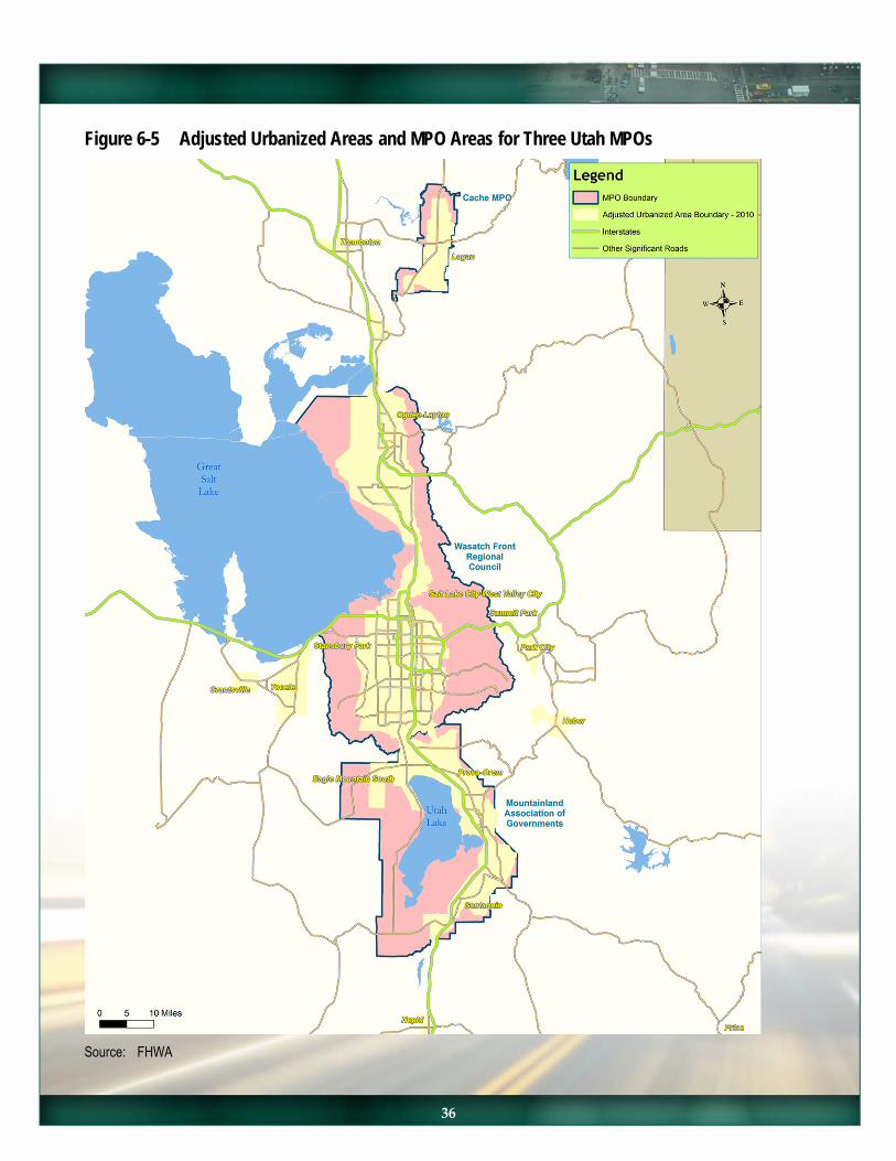
Figure 6-5 Adjusted Urbanized Areas and MPO Areas for Three Utah MPOs

Source: FHWA

36

State records on licensed drivers may help an agency understand the proportion of at-risk drivers. Changes in automobile ownership and driving rates may impact future safety targets as much as countermeasure selection. In 2011, the percentage of 16 to 24 year olds with driver’s licenses dipped to 67 percent—the lowest percentage since at least 1963.23 This seems to indicate that younger drivers may be choosing to delay or not pursue licensure, which reduces their in-vehicle crash exposure. However, they are likely taking transit, which has almost zero risk; or they may be walking or riding a bicycle more often and, therefore, be more exposed to the risks associated with those modes.

Figure 6-6 National Fatalities per 100,000 Population Young Drivers versus Total

Source: Cambridge Systematics, Inc.; FARS; and U.S. Bureau of the Census.

Note: 2013 data are preliminary.

6.4 Modal Trends

Another facet of understanding potential future safety performance is considering the transportation landscape where growth is anticipated. A major consideration is whether transit is available and trends in transit use. If transit is available, the State will want to understand the transit mode share in a State’s urbanized areas. MPOs will be an important resource as they can provide this information for both current conditions and future forecasts from their travel demand models. These forecasts should take into account anticipated investments in transit, pedestrian and bicycle transportation and the extent to which mode shift is anticipated. In general, transit is very safe, so a shift from auto trips to transit will benefit safety. If more people are biking and walking, they will be reducing their risk for crashes in a

23 http://www.uspirg.org/sites/pirg/files/reports/A%20New%20Direction%20vUS.pdf.

0

5

10

15

20

25

30

35

1995 2003 2013*

Age 16 - 24 Total

37

vehicle, but they may be more vulnerable to crashes depending on the state of bicycle and pedestrian infrastructure (i.e., existence of continuous sidewalks or protected bicycle lanes). It will be important to consider mode shift, but if the result of lower VMT growth is more serious crashes involving nonauto modes, safety may not improve overall. It is important to make sure that any changes to the mode share also take into account the share of crashes by mode.

6.5 Safety Culture

An important question to consider for the urbanized areas in a State is the extent to which they have a strong transportation safety culture. To assess this, it is useful to understand the extent to which the MPOs are conducting proactive safety planning, which will have an influence on how safety is considered in regional transportation investments and how aggressive targets should be. A resource for understanding how to consider the extent of safety integration into planning is the Framework for Institutionalizing Safety in the Transportation Planning Process.24 Questions the State can ask regarding MPO safety planning include the following:

• Do MPOs have dedicated safety committees that place a sustained focus on improving safety?

• Have any MPOs developed dedicated safety plans? If so, are they actively implementing them?

• How well is safety integrated into the planning process for the long-range plan, corridor plans, or modal plans:

− Is safety explicit in plan goals and objectives?

− Has the MPO conducted regional analysis of safety problems, such as network screening or identification of safety hot spots?

− Have MPOs developed regional safety targets?25 How aggressive are they? As noted, some metropolitan areas, including New York, Chicago, San Francisco, and Los Angeles, have recently established a high level of commitment to transportation safety as evidenced by their adoption of Vision Zero goals.

− Do the MPOs effectively use safety as a criterion for prioritizing transportation investments? Is safety given sufficient weight relative to other transportation priorities?

− Do MPOs monitor and evaluate performance of the transportation system in terms of safety and reallocate resources as needed?

− Is the region undertaking education and enforcement campaigns to change behaviors and culture related to transportation safety?

If regions are fairly proactive on safety, then a more aggressive urbanized area target might make sense.

24 http://onlinepubs.trb.org/onlinepubs/nchrp/docs/NCHRP08-76_PhaseI-FR.pdf. 25 Under MAP-21, States are required to coordinate with MPOs on development of State targets. MPOs will be

required to set safety targets or adopt the State safety target.

38

6.6 Step 2—Exogenous Factors Example

Now, we will carry the example into the second step of the framework. In Step 1 the statewide target for urbanized areas was 88 fatalities and 323 fatalities for nonurbanized areas. The example State’s analysis shows it should expect more future development in nonurbanized areas than in urbanized areas and, therefore, more nonurbanized VMT, as well as an increasing proportion of drivers over age 65 in nonurbanized areas. As a result, it may be more difficult to make progress on reducing severe crashes in nonurbanized areas. Therefore, the State might want to adjust the target so it is more aggressive in urbanized areas and less aggressive in nonurbanized areas. In this example, the urbanized area target was shifted from a reduction in fatalities of about five annually calculated in Step 1 (red line/gold dots) to a reduction of about six fatalities annually (blue line), so the target is now 82 fatalities by 2012 to 2016 in urbanized areas, as shown in figure 6-7.

Figure 6-7 Sample Step 2—Consideration of Exogenous Factors Urbanized Areas

Source: Cambridge Systematics, Inc.

The target in nonurbanized areas would then be less aggressive, for a decrease in annual fatality reduction from 30 to 29, and the target would be increased from 323 fatalities per year by 2012 to 2016, calculated in step 1 (red line/gold circle) to 328 fatalities per year by 2016, as shown in figure 6-8.

138130 126

118 117 113113107 102 97 92 88

0

20

40

60

80

100

120

140

160

2006 2008 2010 2012 2014 2016 2018

5 Year Average UZA Fatalities Forecast

Targeted annualfatality reduction:

approx. 6

82

39

Figure 6-8 Sample Step 2—Consideration of Exogenous Factors Nonurbanized Areas

Source: Cambridge Systematics, Inc.

6.7 Countermeasure Impact Data

State Data on Countermeasure Effectiveness

States should use the safety analysis tools listed in section 5 to adjust targets. Program and project evaluations help agencies determine which countermeasures are most effective in saving lives and reducing injuries. Agencies should determine which countermeasures have not demonstrated the expected effectiveness and reconsider or modify them in the future. The results of all such evaluations should be captured in a knowledge base to improve future estimates of effectiveness and for consideration in future decision-making and planning. This information is a critical input into evidence-based safety target setting. When a State sets or updates a safety target, it should draw upon its body of knowledge of project effectiveness for use in forecasting future fatality reductions given a set level of resources. This information will help the State develop the most effective safety program possible, and also ensure its fatality targets are realistic.

What is the impact of improvements?

Estimate target based on forecasted fatality reduction

from safety plans

3

Scenario 3

Time

Scenario 1

Safe

ty M

easu

re

Scenario 2

Source: Cambridge Systematics, Inc.

To understand the extent to which a particular measure is working, the State should conduct an evaluation. A range of methods is available for evaluating countermeasures, depending on the available data and resources. Section 6 of the HSIP Manual describes options for conducting project and program evaluation, including before/after analysis. It is critical for the purpose of target setting to continue to improve this information and use it to forecast fatality reductions anticipated from planned safety programs.

628 594552 529

501

442413

200

300

400

500

600

328479

383353

323

0

100

700

2006 2008 2010 2012 2014 2016 2018

5 Year Average Non-UZA Fatalities Forecast

40

Targeted annual fatality reduction: approx. 29

Both individual State DOT and FHWA research have examined countermeasure effectiveness for many years. The CMF Clearinghouse database is a continually updated source for effectiveness data for infrastructure-oriented safety countermeasures. For certain projects, a State may pursue high-quality evaluation that is of the caliber to develop a CMF about the countermeasure. FHWA’s A Guide to Developing Quality Crash Modification Factors is a useful resource. Given the limited number of CMFs currently available, States are encouraged to develop CMFs to contribute to this knowledge base so that fatality reduction forecasts can be continuously improved. This will help States improve the accuracy of target setting. Understanding the urban or rural context of countermeasure implementation also is important.

Data on the effectiveness of behavioral programs is limited and varies according to the scale and type of implementation. For these programs, the best resource is a State’s own evaluation of how the project or program worked on its roadway system. Therefore, States should evaluate projects without known effectiveness data to ensure they are implementing effective programs, and they are getting the most safety improvement possible with the resources available. In-house evaluation generates confidence in the validity of the results and fosters their use in future fatality forecasts and target setting.

Emphasis Area Plans

Through the use of efficacy data (either national CMFs or State-developed information) for multiple projects, a State can develop a detailed emphasis area plan and create reasonable fatality reduction forecasts, provided all countermeasures are implemented. The combination of evidence-based data with a State’s planned safety program will help generate a realistic fatality target, given anticipated resources. Understanding the share of investment planned in urbanized and nonurbanized areas will help with targets for these geographies.

Emphasis area plans should use CMFs or other data on anticipated fatality reductions to forecast the safety benefits of the investment and inform target setting. Two approaches for incorporating CMFs into target setting are: 1) CMFs can be used in individual locations to calculate the forecasted fatality or injury reduction of a specific improvement; and 2) on a systemic level, improvements can be identified throughout a State or area with a history of or high potential for crashes based on identified characteristics. CMFs can be used to forecast the overall reduction in severe crashes within the countermeasure implementation area. The Oregon DOT, in cooperation with the FHWA Resource Center, recently conducted a study that shows how an emphasis area plan can estimate the expected fatality reduction that can be used in target setting, which is described in the following example.

41

Oregon DOT Roadway Departure Safety Implementation Plan

In its Roadway Departure Safety Implementation Plan, Oregon established a roadway departure goal to reduce the seven-year average (2002 to 2008) of 307 roadway departure fatalities by approximately 20 percent by 2016. Achieving this goal will prevent approximately 65 roadway departure deaths from occurring each year.

Oregon combined traditional location-specific strategies with systemic application of large numbers of cost-effective, low-cost countermeasures at locations experiencing specific crash types above a specified frequency level. On some corridors, targeted education and enforcement initiatives were implemented.

Table 6-4 shows a sample of the calculations in the plan, including the number of crashes, as well as the number of annual severe injuries and fatalities the countermeasure was expected to reduce. By dividing the cost of the project by the number of fatalities it is expected to reduce, an estimate is developed of the cost required to save one life per year. This type of analysis is useful in prioritizing projects to ensure the greatest number of fatalities is reduced, given a fixed level of safety investment and in setting targets.

Table 6-4 Oregon Roadway Departure Safety Implementation Plan Countermeasures (Sample)

Countermeasure Approach

Number of

Sections

Associated Costs

($ Million)

Annual Targeted

Crash Reduction

Annual Estimated

Incapacitating Injury

Reduction

Annual Estimated

Fatality Reduction

Required to Save One

Annual Life (Million Dollars)

State Roads Enhanced Curve Sign and Marking Countermeasures—State Rural Roads

Systematic 750 $3.7 112 14.71 7.56 0.49

Enhanced Curve Sign and Marking Countermeasures Plus Flashing Beacons—State Rural Roads

Systematic 20 $0.14 6 0.78 0.41 0.34

Enhanced Curve Sign and Marking Countermeasures—State Urban Roads

Systematic 19 $0.09 8 0.66 0.34 0.26

Enforcement and Education: Alcohol Related—State Roads

Education & Enforcement

36 $1.3 (annual costs) 5 1.11 1.04 6.25

Local Roads Enhanced Curve Sign and Marking Countermeasures—Local Rural Roads

Systematic 442 $4.42 143 15.29 7.39 0.60

Centerline Rumble Stripes—Local Rural Roads

Systematic 88 $3.52 28 1.39 3.17 1.11

Edge Line Rumble Stripes—Local Rural Roads

Systematic 38 $2.30 46 4.63 2.12 1.08

42

Benefit-Cost Analysis

Benefit-cost analysis is a useful approach for providing a relative sense of the fatality reduction results expected for a specific investment. Development of project-specific benefit-cost ratios will help prioritize safety investments for an emphasis area plan. If the projects with the best benefit-cost ratio in a specific emphasis area are chosen for implementation, a State will know it has developed the most effective program possible with defined resources. Once emphasis area plans, including fatality reduction forecasts are developed, they can be used to inform development of a fatality target. The use of benefit-cost analysis, in combination with emphasis area plan development, will help a State know how aggressive the target can be while ensuring it is realistic. Guidance on how to conduct benefit-cost analysis is available in the HSIP Manual.

Urbanized and Nonurbanized Distribution of Safety Problem within Emphasis Areas

An important facet of understanding crash trends and identifying countermeasures to reduce fatalities is knowledge of the most prevalent emphasis areas in urbanized and nonurbanized areas. A few States conduct analysis of the share of the safety problem within an emphasis area in urban and rural areas. This can inform the extent to which countermeasures addressing crashes in that emphasis area are targeted to be urbanized versus nonurbanized areas. If States decide to set urbanized or nonurbanized targets, they will likely want to pay even closer attention to this distribution as they set targets and implement programs.

The study team analyzed FARS data for 2007 to 2011 to determine the proportion of fatalities in each geography by key emphasis areas, which are summarized in table 6-5. At a national level, some emphasis areas for which fatalities occur primarily in urbanized areas include pedestrians (71 percent), bicycles (68 percent), and intersections (68 percent). Emphasis areas dominant in nonurbanized areas include: animal involved (91 percent), unlicensed driver (76 percent), fatigued/asleep (82 percent), and roadway departure (68 percent).

To forecast the extent of anticipated safety progress in urbanized as compared with nonurbanized areas, it is necessary to estimate the level of investment in the two geographies. One way to do this at a broad level is to review the share of fatalities and serious injuries in urbanized and nonurbanized areas within each of the emphasis areas as defined in the SHSP. If future investments are required to align with SHSP emphasis areas, progress should be anticipated in those areas. The State will want to understand whether the future investments are likely to provide more benefit to urbanized or nonurbanized area crashes.

43

Table 6-5 Fatalities by Crash Type in Urbanized and Nonurbanized Areas

National Fatalities

(Annual Average 2007-2011)

Urbanized Area Fatalities

Percent Urbanized Area

Fatalities Nonurbanized Area Fatalities

Percent Nonurbanized Area Fatalities

Alcohol/Drug Impaired 11,461 4,616 40% 6,846 60% Seatbelt/Helmet Not Used/Misused

18,472 7,137 39% 11,335 61%

Distracted/Inattentive Driver 4,886 1,769 36% 3,117 64% Fatigued/Asleep 870 159 18% 711 82% Aggressive 225 103 46% 122 54% Speed Related 10,316 4,162 40% 6,154 60% Pedestrian Killed 4,373 3,109 71% 1,265 29% Bicyclist Killed 668 455 68% 213 32% Motorcyclist Killed 4,840 2,349 49% 2,492 51% Large Truck Involved 1,306 489 37% 817 63% Train Involved 178 59 33% 119 67% Intersection 8,412 4,930 59% 3,481 41% Roadway Departure 20,710 6,726 32% 13,984 68% Work Zone Location 678 319 47% 358 53% Animal Involved 218 19 9% 199 91% Unlicensed Driver 12,429 3,044 24% 9,385 76% Young Driver 5,896 2,309 39% 3,587 61% Older Driver 6,496 2,727 42% 3,769 58% Total 35,371 14,402 41% 20,969 59%

Source: FARS, Cambridge Systematics, Inc.

Table 6-6 shows an example State’s fatalities by emphasis area and the breakdown by urbanized and nonurbanized areas. The total exceeds the actual total of fatalities as each crash may have multiple factors and be represented in multiple emphasis areas. As shown in table 6-6, two-thirds of the fatalities addressed by the emphasis areas are located in nonurbanized areas. Therefore, planned expenditures should have a greater impact on nonurbanized fatality reduction, and the target for the nonurbanized areas should be more aggressive.

44

Table 6-6 Example State Fatalities and Serious Injuries by SHSP Emphasis Area

Emphasis Area Number of Fatalities

in Urbanized Area Number of Fatalities

in Nonurbanized Area Emphasis Area

in SHSP

Alcohol/Drug Related 45 55 Yes Occupant Protection (Safety Belts, Helmets) 53 75 Yes Distracted/Inattentive Driving Related 11 7 Fatigued/asleep 4 17 Aggressive 8 23 Speed Related 12 55 Yes Pedestrian Involved 5 0 Bicycle Involved 6 1 Motorcycle Involved 5 10 Large Truck Involved 9 9 Train Involved 1 0 Intersection/Intersection Related (Signalized and Unsignalized)

62 29 Yes

Roadway Departure: Head-On, Roadside Objects (Trees, Utility Poles), Horizontal Curves

20 205 Yes

Work Zone 2 4 Animal Related 2 0 Unlicensed/Suspended/Revoked License 1 8 Young Driver Involved 30 86 Yes Older Driver Involved 38 16 Share of Total Fatalities and Serious Injuries by Urbanized/Nonurbanized Area

370 (34%) 542 (66%)

Share of Emphasis Area Fatalities and Serious Injuries Addressed by Urbanized/Nonurbanized Area

296 (31%) 431 (69%)

Source: Cambridge Systematics, Inc.

Resource Allocation Data

Resource allocation is a key element of the performance-based planning process. As progress toward achieving targets is made, agencies should engage in a continuous process of reevaluation and reallocation of resources based on where progress is being made and where problems still exist. To understand how investments are affecting progress in urbanized and nonurbanized areas, States should continuously track the level of investment in each of these geographies, as well as fatality and serious injury trends in each geography. Historically, States have not allocated resources to urbanized or nonurbanized areas strictly based on crash trends in these geographies. They have been more likely to invest based on the scale of a safety problem, as compared to the rest of the State or the benefit-cost analysis for an improvement. However, by tracking trends in urbanized and nonurbanized areas, States may learn that they need to reallocate resources to the geography where numbers or rates are

45

experiencing lower levels of progress, or modify how they apply countermeasures in urbanized and nonurbanized areas. For example, if a State determines the majority of its unbelted fatalities and serious injuries are in nonurbanized areas, it will need to ensure that its education and enforcement programs are targeting drivers outside of the urbanized area.

Funding sources have traditionally been limited in their use, and organizational structures have been siloed with infrastructure-oriented funding and countermeasures handled by the State DOT, and behavioral funding and countermeasures handled by the SHSO. This arrangement has made it challenging to shift funding between programs. However, State DOTs now have flexibility to shift HSIP funds to noninfrastructure purposes. Therefore, resource allocation analysis may be even more useful in the future.

6.8 Step 3—Example

In the example, because the SHSP analysis to understand anticipated impact of future investments showed more benefit to nonurbanized areas, the State decides to readjust the nonurbanized target once again to make it more aggressive. Therefore, the end result is to go back to the original trend line shown in Step 1 with a target of 88 fatalities in urbanized areas (figure 6-9) and 323 fatalities in nonurbanized areas by 2012-2016 (figure 6-10).

Figure 6-9 Urbanized Area Fatalities

Source: Cambridge Systematics, Inc.

138130 126

118 117 113113 107 102 97 92 88

y = -4.8258x + 9816.4R² = 0.9562

0

20

40

60

80

100

120

140

160

2006 2008 2010 2012 2014 2016 2018

5 Year Average UZA Fatalities Forecast

Forecasted annual fatality reduction:

approx. 5

46

Figure 6-10 Nonurbanized Fatalities

Source: Cambridge Systematics, Inc.

6.9 Technical Methods

This section describes technical methods and factors to be considered as analysts calculate safety targets.

Selection of Baseline Method

The first consideration when setting a target is what will be used for a base year value against which the target will be compared. Rolling multiyear averages show long-term trends more clearly than annual counts. The longer the time period for which the average is used, however, the longer it will take for trends to show up in the data. If a multiyear average is used, a State or region also will likely track annual numbers.

Projection Methods

To compare fatality targets with fatality trends, a linear regression methodology (also known as a “line of best fit”) is often used to project future fatality numbers and rates. Most spreadsheet software offers a “linear trend” function, which projects what the fatalities would be in the future if the trend were to continue. It is a good idea to review the “fit” of the linear regression. As each fatality becomes more challenging to reduce in the future, it will be more likely that the trend line flattens out as fewer fatalities are reduced per year. Therefore, States may want to segment the trend line to estimate separate linear trends for different time periods; or use nonlinear functions (e.g., exponential, logarithmic, polynomial,

628594

552 529501 479479

442413

383353

323

y = -29.805x + 60410R² = 0.9869

0

100

200

300

400

500

600

700

2006 2008 2010 2012 2014 2016 2018

5 Year Average Non-UZA Fatalities Forecast

Forecasted annual fatality reduction:

approx. 30

47

or power )26 to improve the fit of the trend line with the data. By selecting the R-squared value (in the spreadsheet) to evaluate the fit, different approaches can be compared. The closer the R-squared is to one, the better the fit of the trend line to the historical data.

To adjust a projection further, other statistical methods such as exponential smoothing or averaging can be used. These techniques are helpful because data collected over time will inherently have some form of random variation. “Smoothing” techniques help reveal more clearly the underlying trend, as well as seasonal and cyclic components. More information about smoothing techniques is available in the Engineering Statistics Handbook by the National Institute of Standards and Technology.

Feasibility Assessment

While some targets are set for only one year, others are set for as many as 20 years into the future. A check on the level of ambition for a target is to calculate the annual rate of fatality reduction for both the historical trend and the future years, and to see how they compare. In the future, as the number of fatalities gets closer to zero, every fatality reduction will become more challenging. Therefore, a significantly larger annual reduction than has been achieved in the past may not be realistic. A Compendium of State and Regional Target Setting Practices27 developed calculations of annual fatality reductions for each State where a target was available, and provides a reference for benchmarking. Once a potential target has been defined, agencies should overlay it on the forecasted trend based on past performance. This gives a sense of whether the target seems achievable.

48

26 These methods are available in many off-the-shelf spreadsheet software applications. 27 http://safety.fhwa.dot.gov/hsip/tpm/docs/compendium.pdf.

7.0 Conclusion

The framework for setting statewide safety targets is relevant for urbanized and nonurbanized target setting. However, more complexity is involved when manipulating the data for analysis by the separate urbanized and nonurbanized areas. Additionally, other considerations such as safety culture and urbanization trends must be taken into account when evaluating how aggressive targets should be.

States should consider the quality of their location data before deciding on urbanized and nonurbanized target setting, particularly for serious injuries. If States have lower confidence in accuracy of crash locations, they may want to wait to set urbanized and nonurbanized targets until they have higher confidence in crash locations both on and off the State system.

Urbanized and nonurbanized target setting can help States prioritize their resources for the greatest impact. With increased attention to the locations of crashes, States may be able to tailor implementation of countermeasures better to address the areas with the higher numbers of severe crashes.

Establishment of urbanized and nonurbanized targets may help bring more stakeholders to the process if they feel more of a stake in the targets for their area. Given urbanized areas are part of MPO planning areas, States may find urbanized area target setting improves coordination with MPOs or location jurisdictions.

In terms of evaluation, if the State is monitoring progress by individual urbanized area, it may be able to more quickly recognize when innovative projects and higher level of mode shift are resulting in improved safety outcomes. This could result in improved recognition of how best practices generate results at a regional scale.

49

U.S. Department of Transportation Federal Highway Administration Office of Safety 1200 New Jersey Avenue, SE Washington, DC 20590

FHWA-SA-15-067

June 2015