Urbanisation patterns:European vs. less developed countries*

Diego PugaCentre for Economic Performance,

London School of Economics

CENTRE for ECONOMIC PERFORMANCEDiscussion Paper No. 305, September 1996

ABSTRACT: This paper develops a model in which the interactionbetween transport costs, increasing returns to scale, and labourmigration across sectors and regions creates a tendency for urbanagglomeration. Demand from rural areas favours urbandispersion. European urbanisation took place mainly in the XIXcentury, with higher costs of spatial interaction, weaker economiesof scale, and a less elastic supply of labour to the urban sectorthan in LDCs today. These factors could help explain why primatecities dominate in LDCs, while a comparatively small share ofurban population lives in Europe’s largest cities.

* Thanks to Gilles Duranton, Jan Eeckhout, Paul Krugman, Gianmarco Ottaviano, and Tony Venablesfor helpful discussion, and to referees and the editors of this journal for useful comments andsuggestions. This paper was produced as part of the Programme on International EconomicPerformance at the UK Economic and Social Research Council funded Centre for EconomicPerformance, London School of Economics. Financial support from the Banco de España is gratefullyacknowledged.

KEY WORDS: urbanisation, migration, regional integration, agglomeration.JEL CLASSIFICATION: F12, F15, R12.

Correspondence address:

Diego PugaCentre for Economic PerformanceLondon School of EconomicsHoughton StreetLondon WC2A 2AE, UK

d.puga@lse.ac.uk

http://dpuga.lse.ac.uk

1. Introduction

The less developed countries (LDCs) are experiencing a process of rapid urbanisation.

The fraction of population living in urban areas in these countries increased from 17

to 37% between 1950 and 1990, and is expected to surpass the 50% mark before 2010.

By that time, 77% of the population in the more developed countries is expected to

be urban, still close to the 1990 figure of 73% (United Nations, 1991, table A.1).

The rates of urbanisation in the LDCs are, however, not exceptionally high by

historical standards. The ratio of urban to total population in the LDCs increased from

17 to 26% over the 25-year period from 1950 to 1975 (United Nations, 1991, table A.1).

That is the same increase experienced by now more developed countries over the last

quarter of the nineteenth century (Grauman, 1977; cited in Preston, 1979, p. 37).

While the percentage of urban population in the LDCs is getting closer to that of the

more developed countries, the pattern and size of urban agglomerations are diverging

from what can be observed in the more developed regions, and particularly in

European countries. During the last decades European urban systems have become

increasingly balanced, in the sense that the share of population living in their largest

cities has fallen. The urban sectors of LDCs have instead been absorbed by their largest

cities. In their classic study, Rosen and Resnick (1980) calculate several measures of

urban primacy for the city size distributions of 44 countries (the exponents of Pareto

distributions[1], and also the ratio of each country’s largest city to the sum of the

population of the top five or the top 50 cities). They then investigate several factors

to which urban primacy may be related, and show that countries that are less

developed, have lower transport costs, or export a smaller fraction of their Gross

National Product (GNP) tend to have a larger degree of primacy.

The purpose of this paper is to develop a formal framework suggestive of some

factors that could help explain why more developed, and particularly European,

countries have in general developed more balanced systems of cities than LDCs. The

1 The size distribution of cities is the subject of a massive literature, a large part of whichemphasises the ‘rank-size’ rule: in many countries the number of cities with a population larger thanS is approximately proportional to S –p, where the p (the exponent of this Pareto distribution) is closeto 1. This regularity was brought to the general attention by Zipf (1949) and has given rise to anextensive amount of work (see Carroll, 1982, for a survey; Sheppard, 1982, for a critical account of theliterature on city size distributions; and Richardson, 1978, for a review of proposed theoreticalexplanations for the rank-size rule).

model proposed emphasises the trade-off between increasing returns and transport

costs, traditionally highlighted by central place theory. Lösch (1940), developing the

work of Christaller (1933), already describes the distribution of economic activity as

a compromise between maximising the number of firms operating in a market

(presumably because of some form of aggregate increasing returns) and minimising

transport costs (see Mulligan, 1984, for a review of the literature on central place

theory, and Henderson, 1972, for a critical evaluation of this theory).

Urban economists have built on a similar tension between agglomeration and

dispersion forces, but have generally stressed commuting costs and congestion rather

than transport costs as the main factor limiting urban growth. The distinction can be

regarded as a historical one: commuting costs, land rents and pollution have gained

importance recently, while during early urbanisation it was mainly the need to serve

activities, such as agriculture, which make use of dispersed resources that constrained

city growth.

This paper looks mainly at the early stages of urbanisation, so it focuses on the

costs of serving remote areas as the main force limiting agglomeration. It also argues

that the costs of spatial interaction, and more generally the conditions under which

early urbanisation takes place, may determine urban patterns even after those

conditions change. The main reason for this is the existence of multiple equilibria in

the location of economic activity, which arise from circular causation in the location

decisions of agents: firms and workers tend to locate close to large markets, which are

in turn those where more firms and workers locate (there is a variety of concepts

related to this argument, such as Perroux’s, 1955, ‘growth poles’, Myrdal’s, 1957,

‘circular and cumulative causation’, or Hirshman’s, 1958, ‘forward and backward

linkages’, although its application to regional growth is usually associated with Pred,

1966).

These concepts, while extremely insightful, have found it hard to make their way

into mainstream economic theory. Increasing returns to scale are essential for

explaining the geographical distribution of economic activities (Scotchmer and Thisse,

1992, call this the ‘Folk Theorem of Spatial Economics’). However, it is only recently

that developments in industrial organisation and trade theory have produced the tools

to deal with increasing returns and imperfect competition in a tractable way. Of

2

course, there are ways to get around imperfect competition, the most common of

which is to rely on pure externalities to deal with agglomeration within a perfectly

competitive framework. This strategy has yielded very useful insights on issues like

why there are cities of different sizes and functions, notably in the work of Henderson

(1974, 1988). The down side of relying solely on pure external economies is that one

cannot relate the strength of agglomeration forces to micro features of the economy.

Recent work by Fujita, Krugman, Venables and others has been particularly useful

for understanding how the balance between agglomeration and dispersion forces

relates to microeconomic conditions (Fujita, 1988, 1989; Krugman, 1991a, 1991b, 1993a;

Venables, 1996; Krugman and Venables, 1995a, 1995b, 1996; see Fujita and Thisse,

1996, for a very insightful review of this work). This line of work has also helped

emphasise physical space and the relative location of cities (Fujita and Krugman, 1995;

Fujita, Krugman and Mori, 1995).

This paper builds on that framework, and is most closely related to Krugman

(1991b). He combines a monopolistically competitive manufacturing sector employing

mobile workers with a perfectly competitive agricultural sector employing immobile

farmers. That paper shows how the interplay between increasing returns, transport

costs, and inter-city migration can create a tendency for the spatial agglomeration of

manufacturing activities. While that gives us a useful starting point, the rapid

expansion of urban relative to rural population everywhere suggests that to study

urbanisation patterns one ought to look not only at inter-city migration but also at

rural-urban migration. This is particularly important if one wants to analyse the

differences in urbanisation patterns between European countries and LDCs.

Development economists (e.g., Rosenstain-Rodan, 1943; Lewis, 1954) have long

stressed that the elasticity of labour supply is much higher in LDCs than in more

developed countries, and that this can affect the incentives for industrialisation. In

order to study the effects of different elasticities of labour supply on urban patterns,

this paper avoids the simplifying assumption that manufacturing and agriculture use

totally different factors. It assumes instead that agriculture uses both land and labour,

and that workers move in response to differences in welfare levels both across sectors

and across regions.

3

The remainder of the paper is organised as follows. The next section sets up a two-

region general equilibrium model. Section 3 characterises its equilibria and shows how

the emergence of balanced or primate urban patterns are related to transport costs,

the degree of economies of scale, the strength of demand linkages, and the elasticity

of factor supplies. A final section summarises the main conclusions.

2. The model

Consider an economy with two regions, labelled 1 and 2, and a total population of L

workers. Each region consists of one possible location for a city and an agricultural

hinterland, which has K units of arable land. Each worker is endowed with one unit

of labour and is employed in one of two sectors, urban manufacturing (U) or rural

agriculture (R), in one of the two regions. Let LU,i and LR,i denote respectively urban

and rural populations in region i, for i = 1, 2, so:

(1)L LU,1

LR,1

LU,2

LR,2

.

The distribution of workers between regions and sectors is endogenous and may

change over time through a migration process described below.

Preferences

Consumers have Cobb-Douglas preferences over a constant elasticity of substitution

aggregate of differentiated manufactured goods and a homogeneous agricultural

good. Let γ denote the share of manufactures in expenditure. The indirect utility

function of a consumer working in sector s of region i is

(2)Vs, i

qiγ p

A, i(1 γ ) w

s, i,

4

for s = U, R, and i = 1, 2. Wages in sector s of region i are denoted ws,i, pA,i is the local

price of the agricultural good, and qi is the appropriate price index of manufactures,

defined as

(3)qi≡

⌡⌠

h∈Ni

pM, i, i

(h)(1 σ)

dh ⌡⌠

h∈Nj

τ pM, j, i

(h)(1 σ)

dh1/(1 σ)

,

for i ≠ j. This price index depends on the price of individual varieties and on

interregional transport costs; pM,j,i(h) denotes the free on board price for sales in region

i of variety h manufactured in region j, and Ni is the (endogenously determined) set

of varieties produced at equilibrium in region i. Parameter σ(>1) is the elasticity of

substitution across varieties. Transport costs for manufactures take Samuelson’s (1954)

‘iceberg’ form, so they are incurred in the product itself: τ units have to be shipped

so that one unit reaches the other region. These are broadly defined transport costs,

which represent not just physical transport costs but more generally the costs of doing

business across regions. Landowners have the same preferences as workers, but are

tied to their land.[2]

Rural agriculture

Agriculture is perfectly competitive. It produces under constant returns to scale a

homogenous output, which is costlessly tradeable and will be the numéraire. In each

region the agricultural production function is Cobb-Douglas in land and labour, with

labour share θ. Agricultural output is LR,iθ Ki

(1 – θ), and the rural wage is

(4)wR, i

θL (θ 1)R, i

K (1 θ)i

.

2 Dispersion forces in the model do not rely on this assumption. Even if land rents were not spentlocally, the spatial dispersion of agricultural land ensures that there are agricultural workers (andtherefore some local expenditure on manufactures) everywhere.

5

Urban manufacturing

Manufactures are produced with increasing returns to scale in a monopolistically

competitive industry of the Spence (1976) and Dixit and Stiglitz (1977) type. The total

cost of producing a quantity xi(h) of variety h in city i is

(5)Ci(h) w

iα β x

i(h) .

Production of manufactures therefore involves a fixed labour requirement, α, and a

constant variable labour requirement, β. There is free entry and exit in the

manufacturing industry so, although firms exercise monopoly power, at equilibrium

profits are dissipated.

Migration

Workers migrate in response to differences in welfare levels, so at steady state indirect

utility —as given by expression (2)— is equated across sectors and regions. Off steady

state, migration is assumed to follow the dynamics process

(6)L̇s, i

λj 1,2 r U,R

Ln

Vs, i

Vr, j

Ls, i

Lr, j

,

for s = U, R, and i = 1, 2, where λ > 0. This particular process can be justified by the

following set of assumptions. Opportunities to migrate to sector s of region i arrive

at Poisson rate ρLU,i.[3] When the opportunity arises, a worker migrates only if the

utility level of the representative worker in the sector and region of destination is

higher than his or her own present utility by a factor of at least c. The idiosyncratic

cost of migration c is randomly drawn from a distribution with density function

dF(c) = 1/δc in the interval 1,eδ , and zero elsewhere. Therefore, the probability that

a worker migrates from sector s in region i to sector r in region j when the

opportunity arises is Prob(c < Vs,i/Vr,j) = λLn(Vs,i/Vr,j), where λ ≡ ρ/δ > 0. Net

immigration in sector s of region i then follows the dynamic process described by (6).

3 This is meant to reflect that, as already noted by Ravenstein (1885, p. 199), migrants ‘generallygo by preference to one of the great centres of commerce or industry’.

6

However, any other dynamic process such that workers move to jobs with higher

associated utility levels, and such that steady state utility levels are equalised across

sectors and regions would yield the same analytical results.

General equilibrium

Firms sell in each region, and perceive a constant own price elasticity of σ in every

market. They therefore price output at a constant relative markup over marginal cost.

The profit maximising producer price of manufactures is then identical for all varieties

produced in the same city and proportional to the wage:

(7)pM, i

σβσ 1

wU, i

.

With profits dissipated by free entry and exit, the equilibrium level of output is the

same for every firm:

(8)xα σ 1

β.

Substituting expression (8) into (5) gives the cost for a firm producing in city i as

Ci = wU,i ασ. Urban employment (the population size of city i) is then, by Shephard’s

lemma, proportional to the number of firms in city i (more precisely, to the mass of

local firms), ni ≡ #Ni:

(9)LU, i

ni

∂Ci

∂wU, i

ασni

,

Consumers spend a fraction γ of their income on manufactures, so total expenditure

on manufactures in region i is

(10)ei

γ LU, i

wU, i

LθR, i

K (1 θ)i

.

The first term inside the brackets is the income of urban workers, and the second is

the sum of the income of rural workers and land rents. The demand for an individual

7

variety, xi, can be found by using Roy’s identity on the indirect utility function

—expression (2):

(11)xi

pM, i

σ eiq

i(σ 1) e

jq

j(σ 1)τ (1 σ) ,

for i ≠ j. The free-entry condition,

(12)(xi

x )ni

0 , xi≤ x , n

i≥ 0 ,

for i = 1, 2, closes the short-run equilibrium of the model.

Without loss of generality, let us choose units such that prices equal wages

(βσ = σ – 1), and scale firms such that they earn zero profits at size 1 (achieved by

choosing units such that α = 1/σ). Then, substituting expressions (7) and (9) into (3)

gives the price index in region i as

(13)qi

LU, i

w (1 σ)U, i

LU, j

(τ wU, j

)(1 σ) 1/(1 σ).

Similarly substituting (7) and (8) into (11) yields the urban wage consistent with zero

profits as

(14)wU, i

σ eiq

i(σ 1) e

jq

j(σ 1)τ (1 σ) .

Given an allocation of population across sectors {LU,1, LU,2, LR,1, LR,2}, for known

parameters γ, µ, σ and τ, the short-run equilibrium of the model is a set of wages and

price indices {wU,1, wU,2, wR,1, wR,2, q1, q2} solution to equations (10), (13), and (14) valued

for each of the two regions. Wages and price indices determine short-run welfare

levels —indirect utility, as given by expression (2). If these differ across sectors,

regions, or both, then migration will make the allocation of population change over

time according to the simultaneous differential equation system of expression (6).

In order to understand the location forces captured in the model, it is useful to

consider the following (thought) experiment: if an additional worker locates in a city,

how does this affect the profitability of local firms and the welfare of local workers?

Two types of effects can be distinguished: competition and linkage effects.

Competition effects arise as the presence of an additional firm increases competition

for the local market, thereby lowering the wage that firms in that city can pay without

8

making losses —expression (14). This tends to drive workers out of the city,

eliminating differences in city size. Pushing in the opposite direction there are linkage

effects, which encourage workers and firms to agglomerate. A larger number of

workers brings a larger local expenditure, enabling firms to pay higher nominal

wages, and making the location more attractive for other workers and firms. A larger

number of local workers and firms also implies more locally produced varieties, a

lower price index, and hence higher welfare, attracting more workers into the city and

into the surrounding hinterland —expressions (2) and (3).

The next section shows how the level of transport costs, the degree of economies

of scale, the share of urban goods in consumer expenditure, and the elasticity of

labour supply to the urban sector with respect to rural wages affect the relative

strength of competition and linkage effects. Where linkages dominate, the economy

ends up developing a primate city. Where competition effects dominate, a balanced

urban system tends to emerge.

3. Urbanisation patterns

Let us start by characterising the equilibria of the model in terms of the level of

transport costs, and move on to economies of scale and labour supply later on in this

section. Transport costs have been falling over time (according to Mokyr, 1990,

transport costs for goods fell by 0.88% a year during the first half of the nineteenth

century, a decline that accelerated to 1.5% a year after 1850). The first aim of this

section is to study the effects of this fall in transport costs on urban patterns. Let us

consider two types of candidate equilibria of the model. The first is an equilibrium

with a balanced urban system, characterised by two cities of equal size, each with an

equally populated agricultural hinterland. The second is a pair of equilibria with a

unique primate city (there is a pair of equilibria of this type because the primate city

can be either in region 1 or in region 2).

9

Balanced urban systems

Imagine first a situation where transporting goods is so costly that regions are

essentially autarchic. Without differences in technology or land endowments, the two

regions in our model must be identical. Now think of a gradual reduction in transport

costs over time. With high but finite transport costs, some intraindustry trade takes

place between cities. However, the only stable equilibrium of the model is still

characterised by a balanced urban system, where each of the two cities has the same

share of total population

(15)L

U,1

L

LU,2

Lγ

2 γ θ (1 γ ),

and each city’s hinterland is also equally populated:[4]

(16)L

R,1

L

LR,2

Lθ (1 γ )

2 γ θ (1 γ ).

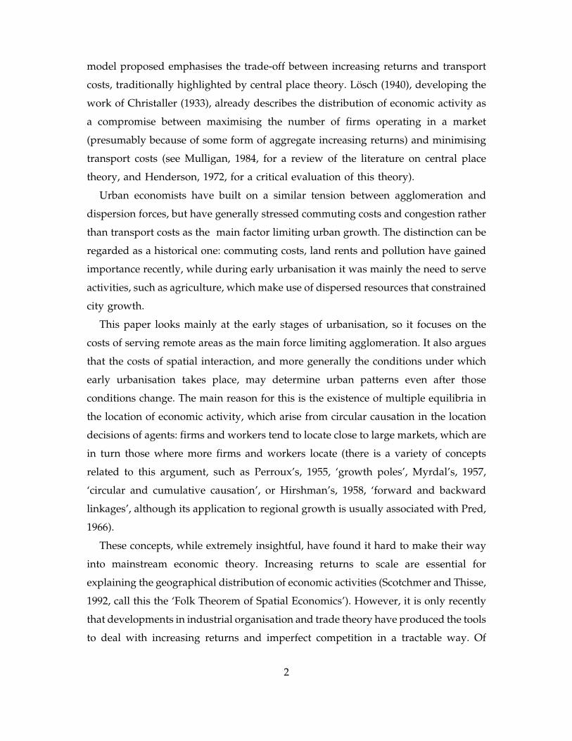
Representing the dynamics of the model graphically is not easy. There are four

state variables in our system of differential equations: the urban and rural populations

in each of the two regions. Total population is held constant (under the assumptions

of the model, the equilibrium share of workers in each sector of each region is

independent of the size of population), so only three of these variables are

independent; let us focus on LU,1, LU,2, and LR,1. This would suggest drawing a three-

dimensional figure with LU,1, LU,2, and LR,1 relative to total population on the axes.

However, three-dimensional figures turn out not to be very helpful in this context. Yet

they can be simplified by taking advantage of the fact that all stable equilibria of the

model lie in the plane LU,1 + LU,2 + 2LR,1 = L (see equations (15) and (16) above, and

(28) and (29) below). Figure 1 has been computed by taking a grid of points on the

intersection of that plane with the unit simplex, and plotting a field of vectors, each

of which has its tail on a point of the grid, is tangent to the phase path crossing that

point, and has module proportional to the speed of convergence to steady state at that

4 The simplest way to calculate these fractions is to choose units such that at the balanced citiesequilibrium wi = qi = Vi = 1, and ni = 1/(1 + τ(1-σ)), ∀i. Expressions (15) and (16) then follow directlyfrom (4), (10), (13) and (14).

10

point. Figure 2 projects the vector field of figure 1 on a plane perpendicular to the LR,1

FIGURE 1Urbanisation dynamics with high transport costs on the plane of equilibria

axis, which gives a two-dimensional representation of the dynamics of the model.

Figures 1 and 2 are drawn for parameter values γ = 0.5, θ = 0.5, σ = 6, and τ = 2.6.

At the unique globally stable equilibrium (labelled B in figure 2), each of the two

cities absorbs one third of total population —as given by expression (15). Although

the size of rural population in each region is not visible in the two-dimensional

projection, expression (16) shows that one sixth of total population lives in the

hinterland of each city at equilibrium.

11

This ‘balanced cities’ equilibrium remains stable as long as transport costs are

0 0.2 0.4 0.6 0.8 1

0

0.2

0.4

0.6

0.8

1

LU,2

LU,1

B

FIGURE 2Urbanisation dynamics with high transport costs

higher than some critical level, making it more profitable to supply rural areas from

a close-by city. This critical level can be determined by linearising the migration

dynamics in the neighbourhood of the balanced cities equilibrium, and using (4), (10),

(13), and (14).[5] The balanced cities equilibrium is a stable node for values of

transport costs higher than the critical value:

(17)τ

B

12γ (2σ 1)

(1 γ ) σ (1 γ ) 1 γ 2η

1/(σ 1)

,

where

5 For details of the derivation of such critical level in this kind of model see Puga (1996).

12

is the elasticity of labour supply to the urban sector with respect to rural wages

(18)η ≡ (1 γ )γ

θ(1 θ )

(valued at equilibrium and in absolute value). When transport costs fall below this

critical value, the balanced cities equilibrium becomes saddle-path unstable. What

drives the change? The balanced cities equilibrium is stable if and only if a

(hypothetical) relocation of a worker, say, from city 2 to city 1 reduces the real wages

of workers in 1 (leading to emigration and firm exit), and increases the real wages of

workers in 2 (leading to immigration and firm entry); it is unstable if the reverse is

true. By relocating from city 2 to city 1, a worker raises the number of varieties

produced in 1, increasing competition for the urban and rural markets of region 1

(and reducing competition for region 2’s markets), thereby lowering the wage that

local firms can afford to pay in 1 without making losses. When transport costs are

high this effect dominates, workers and firms are split between the two cities, and

markets are served mainly on a local basis. When instead transport costs are low,

firms can compete in distant markets without producing locally. The relocation of a

worker from city 2 to city 1 then has little effect on competition but, by lowering the

price index in region 1 and increasing it in 2, it raises relative real wages in city 1 and

its hinterland, attracting migrants from region 2. Immigration also increases local

demand, making local firms able to pay higher wages, which provides further

incentives for immigration. The more workers and firms that move, the more

attractive it is to do so, and this process of circular causation leads to the emergence

of a primate city.[6]

A primate city

When transport costs fall below the critical level of expression (17), what do the

ensuing equilibria look like? Figure 3 is drawn for the same parameter values as

6 Several papers written in the early 1980’s (in particular, three papers reviewed by Dendrinosand Rosser, 1992: Casetti, 1980; Dendrinos, 1980; and Papageorgiou, 1980) address the possibility ofsudden urban growth. Despite the differences with respect to the framework developed in this paper,in all cases discontinuous changes in the equilibrium population distribution arise as the utility gapbetween workers in A and workers in B passes from decreasing locally to increasing locally withmigration from A to B.

13

figures 1 and 2, but with transport costs taking a value (τ = 1.3) below the critical

0 0.2 0.4 0.6 0.8 1

0

0.2

0.4

0.6

0.8

1

LU,2

LU,1

P2

P1

FIGURE 3Urbanisation dynamics with low transport costs

level given by expression (16) (τB* = 1.58). There are now two locally stable equilibria

(labelled P1 and P2), characterised by a single primate city —both are qualitatively

identical but with the role of the regions reversed.

These primate city equilibria are already stable before the balanced cities

equilibrium becomes saddle-path unstable. Therefore, there is some intermediate level

of transport costs for which, if there already is a well-developed system of cities, the

economy converges to the balanced cities equilibrium B; otherwise, a primate city

emerges as the economy converges to equilibria P1 or P2. This configuration with

multiple equilibria is represented in figure 4, drawn for τ = 1.7 —and all other

parameters as figures 1, 2 and 3. Again, it is possible to derive a condition on

parameters under which this configuration appears.

14

Let us focus on equilibrium P1, noting that equilibrium P2 is identical but with

0 0.2 0.4 0.6 0.8 1

0

0.2

0.4

0.6

0.8

1

LU,2

LU,1

B

P1

P2

FIGURE 4Urbanisation dynamics with intermediate transport costs

region labels reversed. At P1 there is no manufacturing production in region 2. This

is an equilibrium only if, when valued at P1, the real wages of a worker hired by a

firm relocating to city 2 are lower than real wages elsewhere in the economy, so the

first firm locating there would be unable to attract workers.[7] Let us check when this

is the case. With all varieties of manufactures produced in city 1 the price indices in

the two regions are

7 There is a parallel between the derivation of the local stability condition for the primate cityoutcome and Rosenstein–Rodan’s (1943) concept of the ‘big push’, formalised amongst others byMurphy, Shleifer and Vishny (1989). According to this view, a firm that wants to settle in a newlocation must pay high enough wages to attract agricultural workers into its factory. However, unlessit can generate enough demand for its production from sources other than its own workers it may notbe able to break even. As in the ‘big push’ literature, multiple equilibria are possible: if firmsproducing different goods invest together, they can sell their output to each other’s workers; and,although it may not have been individually profitable for each firm to make such an investment,coordinated action can allow firms to pay a wage premium, while still breaking even.

15

(19)q1

L 1/(1 σ)U,1

wU,1

, q2

L 1/(1 σ)U,1

wU,1

τ .

By expressions (11) and (19), the highest nominal wage that a deviant firm relocating

to region 2 can pay a worker without making losses compares to the nominal wage

of urban workers in city 1 as given by

(20)

wU,2

wU,1

σe

1

e1

e2

τ (1 σ)e

2

e1

e2

τ (σ 1) .

To turn nominal wages into real wages one must divide by the appropriate price

index (qiγ). Using (19), then shows that the real wages of a worker hired by a firm

relocating to city 2 are lower than real wages elsewhere in the economy (so there is

a locally stable equilibrium at P1) if and only if ν ≥ 1, where

(21)ν ≡

VU,2

V

σ

τ σγ

e2

e1

e2

τ (1 σ)e

2

e1

e2

τ (σ 1) ,

and V is the real wage achieved at equilibrium by any worker elsewhere in the

economy: V ≡ VU,1 = VR,1 = VR,2. The final step is to express the equilibrium shares of

manufacturing expenditure in each region as a function of parameters. At P1 city 1

meets the economy’s demand for manufactures, so

(22)LU,1

wU,1

e1

e2

,

where expenditures on manufactures in each country are, from (10),

(23)e1

γ LU,1

wU,1

LθR,1

K (1 θ) , e2

γ (L LU,1

LR,1

)θK(1 θ) .

Expression (4) gives rural wages as

(24)wR,1

θL(θ 1)R,1

K (1 θ) , wR,2

θ (L LU,1

LR,1

)(θ 1) K(1 θ) .

At equilibrium real wages are equalised so VU,1 = VR,1 = VR,2. This, together with (24),

implies that

16

(25)L LU,1

LR,1

τ γ /(θ 1) LR,1

, wU,1

wR,1

.

From expressions (22)-(25) each region’s share in manufacturing expenditure is:

(26)e

1

e1

e2

τθγ /(1 θ) γ1 τθγ /(1 θ)

,e

2

e1

e2

1 γ1 τθγ /(1 θ)

.

Finally, substituting expression (21) into (26) proves that there is a locally stable

equilibrium at P1 (and another one at P2) if and only if

(27)ν τ σγ

τθγ /(1 θ) γ1 τθγ /(1 θ)

τ (1 σ) 1 γ1 τθγ /(1 θ)

τ (σ 1) ≤ 1 .

Unlike in the balanced cities equilibrium case, turning expression (27) into a closed

form solution for the range of transport costs in which the primate city equilibria are

unstable appears to be impossible. Nevertheless, there are several things to be learnt

from this expression. First, as τ approaches 1 so does ν, and ∂ν/∂τ is negative for τ

close to 1. This implies that for sufficiently low transport costs there is a pair of locally

stable equilibria at P1 and P2. Second, as τ becomes infinitely large, so does ν,

provided that [σ(1 – γ) – 1] – γθ/(1 – θ) > 0.[8] So if economies of scale (which are

higher the lower is σ), the share of manufactures in consumer expenditure (γ), and

the share of labour in agricultural costs (θ) are not too large, the shape of ν as a

function of τ looks like in figure 5.

Denote by τP* (= 2.23 in figure 5, drawn for the same parameter values as previous

figures) the level of transport costs at which ν = 1. For values of transport costs

higher than τP* the balanced cities equilibrium is globally stable (as in figure 2). For

values between τP* and τB

* —expression (17)— the balanced cities equilibrium and the

two primate city equilibria are locally stable (as in figure 4). For transport costs lower

than τP*, the balanced cities equilibrium is saddle-path unstable and the two primate

8 If this condition is not satisfied, ν < 1 for all τ, and the critical value at which the symmetricequilibrium switches from locally stable to unstable —expression (17)— is outside the interval (1,∞).This corresponds to the case where economies of scale, the share of manufactures in expenditure, andthe share of labour in agricultural costs are so high that the balanced city equilibrium is unstable andthe primate city equilibria are stable for all values of transport costs.

17

equilibria are locally stable (as in figure 3).

τ1 1.5 2 2.5 3 3.5

0

0.5

1

1.5

2

νS S

FIGURE 5Range of transport costs in which the primate city equilibrium is locally stable

Note that if there is no labour mobility across sectors (θ = 0, so all labour is

employed by manufacturing while agricultural production relies only on a sector-

specific factor), we are in the case studied by Krugman (1991b). When valued at θ = 0,

expression (27) collapses to the analogous expression derived in that paper. Similarly,

valuing expression (17) at θ = 0 yields an analytical solution to the question of when

is an even distribution of manufacturing a stable equilibrium in Krugman’s (1991b)

paper —an issue which that paper only studies through numerical examples.

Considering this more general setup, where θ can take values other than zero and

where the distribution of labour across sectors is endogenous, will help us clarify

below the role of elastic factor supplies in the economics of agglomeration.

At the primate city equilibrium P1, by expressions (22)–(25), region 1 has a city of

population size

18

(28)LU,1

Lγ

γ θ (1 γ ),

with a more populated hinterland than region 2:

(29)

LR,1

Lθ (1 γ )

γ θ (1 γ ) (1 τ γ /(θ 1)),

LR,2

Lθ (1 γ )τ γ /(θ 1)

γ θ (1 γ ) (1 τ γ /(θ 1)).

This is because agricultural workers living close to the city can buy urban

manufactures at lower prices, so at equilibrium agricultural workers in 2 must make

up for it by producing with a lower labour/capital ratio, which gives them a higher

marginal productivity.

Note that the total size of the urban sector at steady state is the same in the

balanced cities equilibrium as in the primate city equilibria. This is because, starting

from any equilibrium of the model, intersectoral migration raises the utility of

workers in the sector that sees its size diminish and lowers the utility of workers in

the sector that sees its size increase, so the size of each sector tends to go back to its

equilibrium level.

The pecuniary externalities that lead to urban primacy in this model rely on three

crucial elements. The first is the existence of economies of scale internal to

manufacturing firms, which make them produce only in a few locations (in fact,

under the assumptions of the model each firm produces in a single location). The

second is some cost of spatial interaction, which encourages firms and workers to

choose locations that have comparatively good market access, which are in turn

locations where there are relatively many firms and workers. The third important

element is a sufficiently elastic supply of labour to the urban sector, so that the

emerging primate city can draw labour from other cities and especially from the pool

of agricultural workers. This last element has been largely ignored by recent location

models using the Spence-Dixit-Stiglitz framework but is crucial: agglomeration can

occur only if increasing returns activities can draw resources either from other sectors

or from other regions.

19

Primate cities emerge under some conditions and not under others because the

pecuniary externalities created by this combination of internal economies of scale,

transport costs, and elastic factor supplies must be set against the stronger

competition faced by firms in larger cities. The advantage of deriving pecuniary

externalities rather than assuming external economies is that one can study how their

strength varies relative to product market competition with the different conditions

under which urbanisation takes place.

Economies of scale, labour supply, and expenditure shares

So far this section has focused on the transport cost parameter τ, which can be

interpreted as a broad measure of the costs of spatial interaction. The results of this

paper suggest that transport costs can play an important role in determining the

pattern of urbanisation. High transport costs allow a balanced system of cities to

emerge, while low transport costs lead to urban primacy. Let us now look at the

effects of the degree of economies of scale, the share of urban goods in consumer

expenditure, and the elasticity of labour supply to the urban sector.

Differentiating expressions (17) and (27) —the latter valued at ν = 1, hence with

τ = τP*— yields the following comparative statics:

(30)∂τB

∂σ,

∂τP

∂σ< 0 ,

∂τB

∂θ,

∂τP

∂θ> 0 ,

∂τB

∂γ,

∂τP

∂γ> 0 .

Parameter σ has at least two interpretations. It is the elasticity of substitution across

varieties in consumer preferences. At equilibrium, it can also be seen as an inverse

measure of economies of scale —the ratio of average to marginal costs in the model

is σ/(σ–1). Quite intuitively, the tendency of firms to agglomerate in a single city

increases with economies of scale —or with a lower substitutability across products.

The lower the share of labour in agricultural production costs, θ, the more elastic

the supply of labour to the urban sector —expression (18). As shown above, the

interaction of increasing returns to scale, transport costs, and migration creates a

tendency for urban agglomeration. However, agglomeration can only occur if workers

can be drawn from elsewhere. The more elastic supply of labour to the urban sector,

20

the easier it is to draw workers from agriculture without large increases in wages, and

the more likely that the economy ends up developing a primate urban pattern.

Finally, a larger share of manufactures in consumer expenditure also favours urban

primacy through two different channels. First, the weight of the price index of

manufactures in real wages increases with γ (in this sense, it is a measure of the

strength of demand linkages), encouraging workers to migrate into regions where

there are relatively many firms. Second, the elasticity of labour supply to the urban

sector increases with γ, helping a primate city emerge.

European vs. LDC urbanisation

These results may provide some insight into the differences between urbanisation in

Europe and in LDCs. European urbanisation took place mainly in the XIX century.[9]

In XIX century Europe the costs of spatial interaction were higher, economies of scale

were weaker, and the pool of agricultural workers available to the urban sector was

smaller than in LDCs today. The model suggests that this could have helped European

countries develop balanced systems of cities.

Urbanisation in LDCs is taking place under lower costs of spatial interaction and

with stronger economies of scale than in XIX century Europe. This may help explain

the different early urbanisation patterns in Europe and in LDCs. However, while

transport costs in LDCs today are lower than in XIX century Europe, they are still

higher than in modern Europe. Why then have European countries not generally

developed primate urban patterns as well? A possible answer is that, in the presence

of multiple equilibria, temporary differences in the conditions under which

9 According to Bairoch (1988), between 1800 and 1900 the population of European cities increasedfrom 19 million to 108 million (from 12.1% to 38% of total population), compared with an increase from8 million to 19 million (from 10.4% to 12.1% of total population) over the previous five centuries.

21

urbanisation takes place can have permanent effects on urban patterns. However, the

main reason for the sustained differences in urban patterns is probably that there is

a much larger pool of agricultural workers available to migrate into the cities of

today’s LDCs than there was in XIX century Europe. Let us consider these two

arguments in turn.

Imagine two countries urbanising with a time lag between them, with transport

costs falling over time.[10] Assume that urbanisation in one of these countries

(labelled ‘European’) starts when the level of transport costs is high, so the dynamics

of urbanisation are like those represented in figure 2. This ‘European’ country then

starts developing a balanced system of cities. When transport costs fall, transforming

the dynamics of urbanisation into those of figure 4, further urban growth in the

‘European’ country operates on a well-developed urban system (it is already within

the basin of attraction of the balanced cities equilibrium, marked with thin arrows in

figure 4), so its balanced urban pattern is preserved and even strengthened.

Now assume that, on the other hand, the second country (labelled ‘LDC’) only

experiences significant urban growth when transport costs have fallen to the range of

multiple equilibria, as depicted in figure 4. Then, even if the final conditions on

parameters are similar to those of the European economy, a quite different urban can

emerge. Thick arrows in figure 4 mark points from which a primate urban pattern

develops. The smaller the level of urbanisation when transport costs reach this level

(the closer {LU,1, LU,2} to the origin of the axes), the smaller the difference in city sizes

necessary for a primate city to emerge.

While multiple equilibria can provide a formal explanation to the persistence of

balanced urban systems in European countries despite falling transport costs, the main

explanation arising from this framework focuses on the different wage elasticity of

labour supply from agriculture to manufacturing.

The rise in the natural growth rate of population in LDCs lead to over a 250%

growth in agricultural population in LDCs between 1800 and 1980 (despite large rural-

urban migration flows, which made possible an increase in urban population by a

10 One can think of urbanisation in this context as triggered by the switch from a traditionalconstant returns to scale technology to a modern increasing returns to scale technology in theproduction of manufactures, in the tradition of the ‘big push’ literature.

22

factor of 15 over the same period). Since in those 180 years the amount of cultivated

land rose by no more than 40%, agricultural population density almost trebled during

this period and by 1985 each agricultural worker in LDCs had an average of just 1.4

hectares of land at his disposal. This is in contrast with urbanisation in Europe, where

between 1800 and 1880 agricultural population rose by less than 35% while the

extension of cultivated land grew by 10-15%. Over the following three decades

European agricultural population grew very little, and after the 1920’s went into

decline. As a result, the land area available per agricultural worker in Europe rose

from 2.3 hectares in 1920 to around 4 hectares in 1980 (all data from Bairoch, 1988).

The increasing population density in rural areas in LDCs has prevented agricultural

productivity in these countries from reproducing the rise that accompanied XIX

century European urbanisation, despite large rural-urban migration flows. Partly as

a consequence of this different evolution of productivity in each sector, the gap

between urban and rural income in LDCs has widened over the last 40 years (see

Bairoch, 1988).

The results of this paper show that when large rural-urban migration flows have

a small impact on the rural-urban wage gap, primate city patterns tend to emerge. As

the costs of doing business at a distance fall, there is always a tendency for larger

cities to grow disproportionately more than smaller ones (the model shows how this

arises through a circular causation process whereby firms and workers tend to locate

close to large markets, which are in turn those where more firms and workers locate).

However, in order to grow cities need to attract workers, specially from rural areas.

If as agricultural workers flow into the larger cities the advantages of moving there

are reduced fast, balanced urban systems tend to arise, as has happened in Europe.

Instead, when migration does not have a strong negative impact on the incentives for

further migration population in large cities tends to build up, and primate cities

emerge as they have in LDCs.

23

4. Conclusions

The world’s largest metropolises are increasingly located in the poorest regions of the

world. The fraction of population living in urban areas in the less developed countries

(LDCs) is growing closer to that of the more developed regions. Yet the pattern and

size of urban agglomerations in the LDCs are diverging from what can be observed

in the more developed countries, and particularly in Europe. Despite the many

similarities in their urbanisation processes, while the balance between cities in

European countries remains and is even strengthening (their largest cities account for

a small and falling share of urban population), the growing urban sector of the LDCs

is instead being absorbed by its largest cities.

Many economic, geographic, historic, political, and social factors play a role in

explaining why some particular cities are larger than others. Yet one would like to

understand the effect of those economic forces that are not specific to each case, but

that describe a general trend. Our analysis highlights four such forces: the costs of

spatial interaction, the degree of economies of scale, the strength of demand linkages,

and the elasticity of labour supply to the urban sector with respect to rural wages, all

of which can play an important role in determining whether an economy develops a

balanced system of cities or a primate urban pattern.

In the proposed framework urban manufacturing and rural agriculture compete for

workers, which migrate across regions and sectors in response to differences in

welfare levels. The interaction between internal economies of scale, transport costs and

migration creates pecuniary externalities, which encourage manufacturing firms to

cluster in larger cities. On the other hand, the need to serve agricultural workers,

which make use of dispersed land, works against this tendency for primate cities and

favours balanced urban patterns.

Lower transport costs make it easier for firms to supply remote areas from large

cities, and can trigger a circular causation process that leads to urban primacy. The

tendency of firms to agglomerate in a primate city also increases with economies of

scale and with the strength of demand linkages. High transport costs, small economies

of scale, and weak linkages favour instead the emergence of a balanced system of

cities.

24

These results may provide some insight into the differences between urbanisation

in Europe and urbanisation in LDCs. European urbanisation took place mainly in the

XIX century, when the costs of spatial interaction were higher and economies of scale

weaker than in today’s LDCs. This could help explain why European countries have

developed balanced urban systems while primate cities dominate in LDCs. In the

presence of multiple equilibria, these temporary differences in the conditions under

which early urbanisation took place in each case may have had permanent effects on

urban patterns.

The degree of openness of an economy also appears to play an important role in

explaining urban primacy: import substitution policies by LDCs made location in the

metropolis more important, while trade liberalisation has allowed firms to spread out.

It is easy to incorporate openness to trade into this framework, but it has been left

outside since Krugman and Livas (1996) already provide an elegant theoretical

justification, supported by empirical evidence from the Mexican case in Hanson

(forthcoming).

Another factor favouring urban primacy is the differential improvement of

infrastructure favouring the metropolis. LDCs have developed radial transport

networks centred on their primate cities much more often than European countries,

and perhaps this has exacerbated the tendency of LDCs to develop metropolis of

disproportionate size. This is what Krugman (1993b) calls the ‘hub effect’, and has

been explored in a urban context by Fujita and Mori (1996).

However, this paper stresses what may well be the main reason for the sustained

differences in urban patterns: there is a much larger pool of agricultural workers

available to migrate into the cities of today’s LDCs than there was in XIX century

Europe. As the costs of doing business at a distance fall, there is always a tendency

for larger cities to grow disproportionately more than smaller ones. However, for such

clustering to occur cities must be able to draw workers from other cities and from

agriculture without large increases in wages. If as agricultural workers flow into the

larger cities the advantages of moving there are reduced fast, balanced urban systems

tend to arise, as they have in Europe. Instead, when migration does not have a strong

negative impact on the incentives for further migration population in large cities tends

to build up, and primate cities emerge as they have in LDCs.

25

References

Bairoch, Paul. 1988. Cities and Economic Development (Christopher Braider trans.).Chicago: Chicago University Press.

Carrol, G. 1982. ‘National city-size distributions: What do we know after 67 years ofresearch?’ Progress in Human Geography, 6: 1-43.

Casetti, Emilio. 1980. ‘Equilibrium population partitions between urban andagricultural occupations.’ Geographical Analysis, 12: 47-54.

Christaller, Walter. 1966. Central Places in Southern Germany (Carlisle W. Baskin trans.).Englewood Cliffs, NJ: Prentice Hall.

Dendrinos, Dimitrios S. 1980. ‘Dynamics of city size and structural stability: The caseof a single city.’ Geographical Analysis, 12: 236-244.

Dendrinos, Dimitrios S. and J. Barkeley Rosser, Jr. 1992. ‘Fundamental issues innonlinear urban population dynamic models: Theory and a synthesis.’ Annals ofRegional Science, 26: 135-145.

Dixit, Avinash K. and Joseph E. Stiglitz. 1977. ‘Monopolistic competition and optimumproduct diversity’, American Economic Review, 67: 297-308.

Fujita, Masahisa. 1988. ‘A monopolistic competition model of spatial agglomeration:A differentiated product approach.’ Regional Science and Urban Economics, 18: 87-124.

Fujita, Masahisa. 1989. Urban Economic Theory, Land Use and City Size. Cambridge:Cambridge University Press.

Fujita, Masahisa and Paul R. Krugman. 1995. ‘When is the economy monocentric? vonThünen and Chamberlin unified.’ Regional Science and Urban Economics, 25: 508-528.

Fujita, Masahisa, Paul R. Krugman and Tomoya Mori. 1995. ‘On the evolution ofhierarchical urban systems’, Discussion Paper No. 419, Institute of EconomicResearch, Kyoto University .

Fujita, Masahisa and Tomoya Mori. 1996. ‘The role of ports in the making of majorcities: Self-agglomeration and hub-effect.’ Journal of Development Economics, 49: 93-120.

Fujita, Masahisa and Jacques-François Thisse. 1996. ‘Economics of Agglomeration.’Journal of the Japanese and International Economies, 10: 339-378

Grauman, John V. 1977. ‘Orders of magnitude of the world’s urban and ruralpopulation in history.’ United Nations Population Bulletin, 8: 16-33.

Hanson, Gordon H. Forthcoming. ‘Increasing returns, trade, and the regional structureof wages.’ Economic Journal.

Henderson, J. Vernon. 1972. ‘Hierarchy models of city size: An economic evaluation.‘Journal of Regional Science, 12: 435-441.

Henderson, J. Vernon. 1974. ‘The sizes and types of cities.’ American Economic Review,64: 640-656.

26

Henderson, J. Vernon. 1987. ‘General equilibrium modelling of systems of cities.’ InEdwin S. Mills (ed.). Handbook of Regional and Urban Economics, 2. Amsterdam:Elsevier: 927-956.

Hirshman, Albert O. 1958. The Strategy of Economic Development. New Haven,Connecticut: Yale University Press.

Krugman, Paul R. 1991a. Geography and Trade. Cambridge, MA: MIT press.

Krugman, Paul R. 1991b. ‘Increasing returns and economic geography.’ Journal ofPolitical Economy, 99: 483-499.

Krugman, Paul R. 1993a. ‘First nature, second nature and metropolitan location.’Journal of Regional Science, 33: 129-144.

Krugman, Paul R. 1993b. ‘The hub effect: or, threeness in interregional trade.’ InWilfred J. Ethier, Elhanan Helpman, and J. Peter Neary (eds.). Theory, Policy andDynamics in International Trade. Cambridge: Cambridge University Press: 29–37.

Krugman, Paul R. and Raúl Livas Elizondo. 1996. ‘Trade policy and the third worldmetropolis.’ Journal of Development Economics, 49: 137-150.

Krugman, Paul R. and Anthony J. Venables. 1995a. ‘Globalization and the inequalityof nations.’ Quarterly Journal of Economics, 110: 857-880.

Krugman, Paul R. and Anthony J. Venables. 1995b. ‘The seamless world: a spatialmodel of international specialisation.’ Discussion Paper No. 1230, Centre forEconomic Policy Research.

Krugman, Paul R. and Anthony J. Venables. 1996. ‘Integration, specialization andadjustment.’ European Economic Review, 40: 959-968.

Lewis, W. Arthur. 1954. ‘Economic Development with unlimited supplies of labour.’The Manchester School, 22: 139-191.

Lösch, August. 1954. The Economics of Location. New Haven, CT: Yale University Press.

Mokyr, Joel. 1990. The Lever of Riches. Oxford: Oxford University Press.

Mulligan, Gordon F. 1984. ‘Agglomeration and central place theory: a review of theliterature.’ International Regional Science Review, 9: 1-42.

Murphy, Kevin M., Andrei Shleifer, and Robert W. Vishny. 1989. ‘Industrializationand the big push.’ Journal of Political Economy, 97: 1003-1026.

Myrdal, Gunnar. 1957. Economic Theory and Under-developed Regions. London:Duckworth.

Papageorgiou, G. J. 1980. ‘On sudden urban growth.’ Environment and planning A, 12:1035-1050.

Perroux, François. 1955. ‘Note sur la notion de pôle de croissance.’ Economiqueappliquée, 1-2: 307-320.

Pred, Alan R. 1966. The Spatial Dynamics of US Urban-Industrial Growth, 1800-1914:Interpretive and Theoretical Essays. Cambridge, MA: MIT press.

27

Preston, Samuel H. 1979. ‘Urban growth in developing countries—a demographicappraisal.’ Population and Development Review, 5: 195-215.

Puga, Diego. 1996. ‘The rise and fall of regional inequalities.’ Discussion Paper No.314, Centre for Economic Performance, London School of Economics.

Richardson, Harry W. 1973. ‘Theory of the distribution of city sizes: Review andprospects.’ Regional Studies, 7: 239-251.

Rosen, Kenneth T. and Mitchel Resnick. 1980. ‘The size distribution of cities: Anexamination of the Pareto law and primacy.’ Journal of Urban Economics, 8: 165-186.

Rosenstein-Rodan, Paul N. 1943. ‘Problems of industrialisation of Eastern and South-eastern Europe.’ Economic Journal, 53: 202-211.

Samuelson, Paul A. 1954. ‘The transfer problem and transport costs, II: Analysis ofeffects of trade impediments.’ Economic Journal, 64: 264-289.

Scotchmer, Susan and Jacques-François Thisse. 1992. ‘Space and competition: APuzzle.’ Annals of Regional Science, 26: 269-286.

Sheppard, Eric. 1982. ‘City size distributions and spatial economic change.’International Regional Science Review, 7: 127-151.

Spence, Michael. 1976. ‘Product selection, fixed costs, and monopolistic competition.’Review of Economic Studies, 43: 217-235.

United Nations. 1991. World Urbanization Prospects 1990. New York: United Nations.

Venables, Anthony J. 1996. ‘Equilibrium locations of vertically linked industries.’International Economic Review, 37: 341-359.

Zipf, George Kingsley. 1949. Human Behaviour and the Principle of Least Effort: AnIntroduction to Human Ecology. Cambridge, MA: Addison Wesley.

28