Urban Sprawl and Social Capital:Evidence from Indonesian Cities∗

Andrea CivelliUniversity of Arkansas

Arya GaduhUniversity of Arkansas

Alexander D. Rothenberg†Syracuse University

Yao WangSyracuse University

February 2021

Abstract

We use detailed data from cities in Indonesia to study the relationship between urban sprawl andsocial capital. For identification, we combine instruments for density with controls for communityaverages of observed characteristics, which control for sorting on observables and unobservables. Wefind that lower density increases trust in neighbors and community participation in urban areas ofIndonesia, but it is also associated with lower interethnic tolerance. Heterogeneity analysis suggeststhat these findings are not explained by differential opportunity costs, but are instead reflective ofsocial forces, including overall ethnic diversity and crime rates.

JEL Classifications: R11, D71, H41

Keywords: urban sprawl, social capital, neighborhood effects

∗We thank seminar participants at Le Moyne College, the 2020 Virtual Meeting of the Urban Economics Association, andSyracuse University. All errors remain our own.†Corresponding author: 426 Eggers Hall, Syracuse, NY 13244-1020. Email: adrothen@maxwell.syr.edu.

1

1 Introduction

In many developing countries, urbanization is proceeding at an astonishing pace. The number of peopleliving in urban areas in Asia increased by more than a billion from 1980 to 2010, and that same figure forAfrica is expected to triple between 2018 and 2050 (ADB, 2012; UN, 2019). As rural to urban migrationand rising incomes attract millions to cities in lower-to-middle income countries (LMICs), many of thosecities are sprawling rapidly. Globally on average, cities are expanding spatially at twice their populationgrowth rates (Angel et al., 2011).

Rapid urban sprawl raises concerns that low-density development may lead to the loss of a sense ofcommunity or more generally, social capital. Critics of urban sprawl have argued that compact, denseurban areas are more likely to promote social interaction (Jacobs, 1961), and because sprawl increasescommuting times, it raises opportunity costs for community participation and interactions with neigh-bors (Putnam, 2000). Moreover, when sprawling development in the urban periphery offers new oppor-tunities for sorting, the clustering of like-minded individuals may increase political polarization (Bishop,2009).1 If lower density erodes social capital and a sense of community, policies to reduce sprawl andmitigate these negative social externalities may be justified (Brueckner and Largey, 2008).2

However, it is not clear that low-density development will necessarily erode social capital. For in-stance, an older tradition in sociology, associated with the works of Simmel (1903) and Wirth (1938),argues that urban life overloads the senses, leading urban residents to limit social interactions withneighbors to preserve their mental energy. Trust may be harder to sustain in denser communities asanonymous interactions among people with diverse backgrounds and little shared norms increase (Hab-yarimana et al., 2007). Moreover, when density is associated with higher crime levels, its negative impacton trust and social capital might become amplified. On the other hand, density could instead facilitategreater intergroup interactions which could foster mutual understanding (Bazzi et al., 2019).

Although correlates of density and social interaction have been well studied in the U.S. and Europe(e.g. Glaeser and Gottlieb, 2006; Brueckner and Largey, 2008), little is known about how low-density de-velopment affects social capital in cities from low- and middle-income countries (LMICs). In this paper,we revisit the relationship between density and social capital, using uniquely rich data from cities inIndonesia, a middle-income and ethnically diverse country that has experienced rapid industrialization.To study multiple dimensions of social capital, we use cross-sectional data from the 2012 National So-cioeconomic Survey (Survei Sosial Ekonomi Nasional, or Susenas). This survey provides detailed measuresof various aspects of social capital, including trust in neighbors, community participation, and intereth-nic tolerance. Such measures reflect both “bonding” social capital, or within-group trust, and “bridging”social capital, or greater ties across groups (Putnam, 2000). We also use similar measures from a panel ofhouseholds in the Indonesia Family Life Survey (IFLS).

In studying how urban sprawl affects social capital, we confront two fundamental identificationchallenges: simultaneity and sorting. The first identification problem is that social capital and densitymay be determined simultaneously, and omitted, place-specific characteristics may drive correlations in

1Growing political polarization has been a feature of many LMICs with democratic governments, including Brazil, India, andIndonesia (Carothers and O’Donohue, 2019).

2Related theoretical work has also argued that sprawl may reduce social interactions and increase segregation between groups,impacting equilibrium levels of employment (Sato and Zenou, 2015; Picard and Zenou, 2018).

2

both variables. An example of this “simultaneity problem” is that unobserved geographic or naturalamenities may both facilitate cooperation over the provision of local public goods and also attract morepeople. The second identification problem is that people who differ in their willingness to contributeto local social capital may sort differentially into areas with different degrees of density. For instance,people with a strong dislike of other ethnic groups may sort into more homogeneous areas which tend tobe less dense. Both identification problems make it challenging to draw causal inferences from observedcorrelations between population density and social capital measures.

Prior research has confronted the simultaneity problem by instrumenting for population density.For example, Brueckner and Largey (2008) use terrain ruggedness in the urban fringe and populationdensity at a higher level of aggregation to instrument for census tract density. We follow a similar ap-proach, instrumenting population density in Indonesian communities using two sets of variables: (1)soil characteristics, which were determined millions of years ago and influenced historical settlementpatterns; (2) satellite-derived measures of built up areas in 1975, when Indonesia was still in the pro-cess of industrializing. Although these instruments differ in their coverage, sources of variation, andexclusion restrictions, they both have a strong first-stage relationship with density.

However, previous studies of the relationship between sprawl and social capital have not adequatelyaddressed the second identification challenge, namely that sorting could still be confounding estimates,even if simultaneity is addressed. To tackle sorting, we combine our instruments for density with con-trols for community-level averages of observed individual characteristics. We include a rich vector of 38controls for observed population and demographic characteristics, computed from 2010 census micro-data. Altonji and Mansfield (2018) show that under certain assumptions, these controls for sorting onobservables will also control for sorting on unobservables. We show that by combining their approach— which obtains partial identification of group-level treatment effects — with instrumental variables,we can point-identify the effects of density unconfounded by sorting or simultaneity.

We find that reductions in density increase trust in neighbors and community participation, echoingthe findings of Brueckner and Largey (2008). These results are robust to controlling for sorting andsimultaneity using different sets of instruments. However, we also find that lower density is correlatedwith reduced intergroup tolerance and cooperation, suggesting a potential negative social externality ofsprawl. This latter result is somewhat less robust than the findings on trust and community participation,suggesting that sorting may play more of a role in driving these findings. Our results are robust todifferent specifications, and we find similar results when we use different data to test these hypotheses.

Our finding that greater density reduces within-village trust and community participation contra-dicts the hypothesis that variation in these forms of social capital is driven by higher opportunity costsfor social interactions (Putnam, 2000; Glaeser and Gottlieb, 2006). A heterogeneity analysis based onproxies for individual-level opportunity costs further rejects this hypothesis. For example, if oppor-tunity costs were important, it would be harder for wealthy individuals to participate in low density,suburban communities, attenuating the negative relationship between density and community partici-pation for those individuals. Instead, we find even more negative effects of density on social capital forwealthier individuals. This result is robust to using other proxies for greater opportunity costs of time atthe individual level, such as being married, having higher education, or commuting using a private mo-tor vehicle. We also find more negative effects of density in more expansive and more rapidly sprawling

3

cities, further contradicting the opportunity costs hypothesis.On the other hand, we find that the relationship between density and social capital is more pro-

nounced in cities with greater ethnic diversity. In such cities, greater sprawl may facilitate sorting ofsimilar individuals into homogenous ethnic enclaves, increasing aspects of bonding social capital likecommunity trust and participation. However, at the same time, these homogenous communities mayalso weaken interethnic tolerance and erode bridging social capital. We also find more pronounced ef-fects of density on social capital in higher crime cities. This provides support for the idea that densityreduces social capital because crime in dense areas increases fear, undermining trust and communityparticipation (Glaeser and Sacerdote, 1999).

To better understand why lower density communities have greater levels of trust and communityparticipation, even after accounting for sorting, we study an evolutionary trust game, following Manapatet al. (2013). In the model, individuals from different ethnic groups interact repeatedly by playing trustgames with different members of their community, either as an investor or a trustee. An investor’spotential return from trusting a co-ethnic trustee exceeds that from trusting a non co-ethnic trustee. Invery dense communities, interactions are more likely to be anonymous, and players are less likely tohave information about what strategies their opponents will play. This reduces the overall level of trustin equilibrium. Simulation results confirm that less information weakens trust, an effect that is robustto differences in ethnic composition. We also use the model data to effectively control for sorting inestimating the relationship between density and trust outcomes as we do in the empirical work.

Since the groundbreaking work of Putnam (2000), a large empirical literature that spans multipledisciplines tries to estimate the impact of urban sprawl on social capital outcomes, but existing evi-dence is mixed. Many studies find a negative relationship between various aspects of urban sprawl andsocial capital, but these results are difficult to interpret because they do not adequately address chal-lenges of causal inference.3 More recent studies have attempted to address the endogeneity of sprawlmeasures, such as density, through the use of instrumental variables or other methods. Although thesestudies do not tackle sorting, they tend to find that social capital is lower in higher density communities.4

Our estimates, which use both instruments for density and controls for sorting, represent a significantmethodological improvement over prior research.

We also contribute to the scarce literature studying the relationship between urban sprawl and socialcapital in developing country cities. With worse traffic congestion and lower-quality public transporta-tion infrastructure, the potential impact of sprawl on social capital in LMICs could be even larger thanin high-income countries. The few existing quantitative empirical papers on sprawl and social capitalin LMICs, including Hemani et al. (2017) on neighborhood forms and social capital in Assam, India,and Zhao (2013) on segregation and sprawl in Beijing, suffer from identification problems. Anotherbody of research uses qualitative methods, such as Connell (1999) on social isolation and sprawl in inManila, Philippines, Caldeira (2001) on social segregation and fear in Sao Paolo, Brazil, and Coy andPohler (2002) on gated communities in Latin American cities. Our paper represents some of the best

3Prominent examples include Freeman (2001) on U.S. cities in the early 1990s, Leyden (2003) on the effects of walkable neigh-borhoods in U.S. cities, Besser et al. (2008) on commuting times and socially oriented trips, Wood et al. (2008) and Wood et al.(2012) on the impact of neighborhood design and social interactions in Western Australia, and Glaeser and Sacerdote (2000)on the impact of living in large apartment buildings.

4Examples of studies focusing on the United States and using instruments for density or other approaches to address thesimultaneity problem include Glaeser and Gottlieb (2006), Brueckner and Largey (2008), and Nguyen (2010).

4

quantitative evidence on sprawl and social capital from a non-upper income context.5

The rest of this paper is organized as follows. Section 2 presents background information on ur-banization and economic development in Indonesia. It also provides an overview of ethnic diversityand different aspects of social capital that are important for our analysis. Section 3 describes the differ-ent datasets we analyze. Section 4 explains how we define metropolitan areas, how we measure urbansprawl, and presents some evidence on correlates of sprawl. Section 5 describes our empirical strategy,extending the work of Altonji and Mansfield (2018), which enables us to address the two identificationproblems in studying the relationship between urban sprawl and social capital. Section 6 presents re-sults of estimating the impact of population density on social capital from multiple datasets. Section 7presents an evolutionary game theory model that sheds light on a key mechanism relating density totrust outcomes. Section 8 concludes.

2 Background

After a sustained period of economic growth and structural transformation since the late 1960s, Indone-sia is now an upper-middle income economy. From 1970 to 1997 (immediately before the Asian FinancialCrisis), per-capita GDP grew by approximately 4.4 percent a year, from just $772 in 1970 (in constant 2010USD) to just over $2,400 in 1997. This sustained growth was accompanied by rapid structural changeas agriculture’s share of GDP rapidly declined, while the share of manufacturing and services grewdramatically (Hill, 1996).

As the structure of Indonesia’s economy transformed, people increasingly migrated out of rural ar-eas, leading to rapid urbanization. In the 1980s and 1990s, the country’s urbanization rate grew by 3percent a year—an even faster rate of urban growth than was experienced by many other East Asiancountries, including China. Between 1990 and 2000, the rate of urban growth in Indonesia peaked, andthe subsequent two decades saw much slower urban growth. The population living in urban areas morethan doubled between 1970 and 2010, and today, about 151 million (or 56 percent) of Indonesians livein urban areas (Roberts et al., 2019). By 2045, when Indonesia will celebrate its centennial, approxi-mately 220 million people are expected to live in urban areas, amounting to more than 70 percent of thepopulation.

As urban growth continues, many Indonesian cities have experienced significant spatial expansion.Economic activities in the largest cities have sprawled well beyond their administrative borders, leadingto the formation of agglomerations that span multiple districts.6 This outward expansion has led to sig-nificant growth in the periphery of urban areas. Although the high economic productivity in urban coresattracted significant migration and growth, housing costs increased rapidly, and many urban residentsrelocated to the periphery. Indeed, between 2000 and 2010, about one-third of population growth in theperipheries of metro areas has come from migration (Roberts et al., 2019, Figure 1.12).

5In a recent paper, Muzayanah et al. (2020) also study sprawl and social capital outcomes in Indonesian cities using similardata as we do, but our methodologies differ substantially. As we do, they find that individuals living in higher density areashad lower levels of trust, were less likely to know their neighbors, and were less involved in community activities. But theydo not look at interethnic tolerance, and they use multi-level logistic regression, failing to address any endogeneity issues.

6Roberts et al. (2019, Box 1.5) identified a total of 21 multidistrict metro areas, defined as metro areas whose labor markets spanmultiple districts.

5

Although variation in the extent of urban sprawl across cities is driven by geo-climatic and socio-economic characteristics, national development policies also played an important role (Civelli and Gaduh,2018). For example, Indonesian policymakers have generally enacted policies favoring motor vehicles,including subsidizing the price of gasoline and investing in road construction, instead of making pub-lic transportation investments. At the same time, agencies responsible for managing land use and ur-ban planning have generally been ineffective in implementing spatial plans and zoning regulations thatcould potentially limit sprawl (Rukmana, 2015).7

2.1 Social Capital and Diversity

Following Putnam (1995), we define social capital as the features of social life, including social networks,social norms, and trust, that enable community members to act together effectively to pursue shared ob-jectives.8 Using a set of indicators that capture this notion of social capital, Legatum Institute (2019a)ranked Indonesia 5th out of 167 countries.9 Indonesia received this high ranking despite its ethno-religious diversity: it is one of the world’s most diverse countries, with more than 1,200 self-identifiedethnic groups whose members belong to one of six recognized religions.10 In 2010, its national-level eth-nic fractionalization index—the probability that any two residents, randomly-drawn from the nationalpopulation, belong to different ethnicities—is around 0.81.

Indonesia’s high ranking on the social capital index amidst its national diversity may appear to con-tradict an extensive empirical literature documenting the negative association between ethnic diversityand social capital (e.g. Alesina and La Ferrara, 2002, 2000; Costa and Kahn, 2003; Putnam, 2007). How-ever, these contradictions disappear once we look at the local level. First, despite its national diversity,most Indonesian communities are very homogeneous, explained in part by the nation’s archipelagic ge-ography, which has separated ethnic groups by vast waterways for centuries. The median Indonesianvillage has a very low ethnic fractionalization index of 0.04. Second, the negative association betweendiversity and social capital resurfaces when we look at variations within Indonesia (Mavridis, 2015;Gaduh, 2016). Ethnic and religious tensions between groups have occasionally sparked violent conflictsthroughout Indonesian history (see, e.g., Bertrand, 2004) and such conflicts are more likely when ethnore-ligous groups are residentially clustered (Barron et al., 2009). Finally, the extent to which local diversitynegatively affects social capital depends on whether diversity makes local inter-group competition moresalient (Bazzi et al., 2019).

A variety of socio-cultural institutions foster social interactions at the local level, particularly in rural

7In a review of its experiences with urban planning, Rukmana (2015) finds that only 8 percent of the land permitted for housingin West Java was complaint with spatial plans. He argued that spatial planning was used to accommodate new developmentand to benefit real estate developers connected to the late Suharto’s regime, rather than to control undesirable development.

8This definition is consistent with DiPasquale and Glaeser (1999), who argue that while social capital does not directly enterthe utility function, it enhances the ability of neighbors to enjoy private investments in local amenities, such as communityorganizations, social groups, or local public goods.

9The Legatum Institute uses survey responses to construct a country-level social capital index that captures “the personal andfamily relationships, social networks and the cohesion a society experiences when there is high institutional trust, and peoplerespect and engage with one another” (Legatum Institute, 2019b, p.7). The index is aggregated from the following sub-indices:(i) personal and family relationships; (ii) social networks; (iii) interpersonal trust; (iv) institutional trust; and (v) civic and socialparticipation. Data for the social capital index come primarily, but not entirely, from the Gallup survey.

10The Indonesian government only recognizes six belief systems to be religions: (1) Buddhism; (2) Catholicism; (3) Confucian-ism; (4) Hinduism; (5) Islam; and (6) Protestantism.

6

areas. For example, “Gotong royong” is a norm of mutual and reciprocal assistance rooted in village,agrarian societies across Indonesia (Bowen, 1986). It encourages collective activities at the communitylevel, such as mutual insurance, public good provision, collective work (e.g., harvesting), as well ascelebrations (births and weddings) and commiserations (funerals) (see, e.g., Koentjaraningrat, 1985).Many of these social activities are organized by social, religious, or village-government organizationsin the communities. Others, such as mutual insurance through arisan (i.e., rotating savings and creditassociation or ROSCA), were often developed organically by individual members.

Local-level institutions, and the social capital they generate, can help fill in some of the gaps inpublic goods left by the Indonesian government, both in rural and urban communities (Woolcock andNarayan, 2000; Bebbington et al., 2006). Many ethnic and religious institutions can naturally be foundin both rural and urban communities. However, as cities expand into previously rural communities,the melding of rural and urban communities — what McGee (1991) describes as “desakota” (village-city)— means that some of the social institutions originating in rural areas (e.g., collective maintenance ofpublic goods, mutual insurance) can also be found in many of Indonesia’s urban communities (Beardand Dasgupta, 2006). Moreover, there is evidence that social interactions remain vibrant in these urbancommunities (Jellinek, 1991; Wilhelm, 2011). Miguel et al. (2006) found that rapid industrialization inIndonesia was positively associated with social capital within these industrializing regions, albeit at thecost of decreased social capital in neighboring regions.

3 Data

To study the relationship between social capital and urban sprawl in Indonesia, we combine severalhigh-quality data sources. These include social capital measures from household survey data, popula-tion census data, and geospatial datasets. We briefly describe each of these data sources in turn.

Social Capital Measures. Our primary source of social capital outcomes is the 2012 National Socioeco-nomic Survey (Survei Sosial Ekonomi Nasional, or Susenas). The 2012 Susenas contains a detailed modulethat asked household-head respondents several questions about different aspects of social capital. Thesevariables, described and summarized in Table 1, have been grouped into three broad categories. Panel Alists the set of questions asks about how well individuals trust their immediate neighbors, an importantdimension of local social capital. Panel B lists the set of questions to measure participation in commu-nity activities and trust in community leadership. Panel C includes measures of tolerance in intergrouprelations.

Our main specifications include responses to these questions for roughly 20,000 households livingover 1,900 communities (desa or kelurahan). The community is the lowest administrative unit in Indone-sia and comprises our main spatial unit of analysis.11 Our sample of Susenas data contains observationsthat span 27 of Indonesia’s 34 provinces. Our main analysis focuses on estimates of the mean effects ofdensity on these outcomes, following Kling et al. (2007) as described below. Because most social capitalresponses are recorded on a 4 or a 5 point scale, we also use models that account for the ordered nature ofthese limited dependent variables in our analysis. In addition, the Susenas data also contain many mea-

11According to Census data, the communities in our sample had an average population of 9,766 in 2000 and 11,462 in 2010.

7

sures useful for individual-level controls, including age, education, marital status, employment sector,and employment status.

Community-Level Demographic Characteristics. We construct community-level demographic char-acteristics with data from the 2000 and 2010 Population Censuses. The census data allow us to constructmultiple measures of average characteristics at the community level, including the size of the local pop-ulation, the share of community members with different levels of educational attainment, and the sharewith different types of marital or migration status. The data also include questions on ethnicity, religion,and census block information that we can use to construct diversity and segregation measures.12 As wedescribe below, community-averages of individual-level characteristics, which are calculated from thesedata, are crucial for our empirical strategy.

Soil Quality Data. We use data from SoilGrids to measure the characteristics of soils prevalent in In-donesian communities. SoilGrids is a global dataset that combines soil profile input data from roughly150,000 sites with machine learning algorithms to provide global, 250-meter resolution predictions ofmany standard soil properties (Hengl et al., 2017).13 These properties include (1) bulk density; (2) watercontent; (3) sand content; (4) clay content; (5) texture classification; and (6) soil taxonomy information.14

Although measures of organic carbon content and soil pH are also available, we did not use these mea-sures in our analysis, because they can be directly manipulated by human activity. We also only usedmeasures for soil characteristics at a depth of 60 cm or more, as these capture variation in the subsoilsand parent material of soils which were largely determined millions of years ago. Because we collected alarge vector of soil characteristics, we use post-double-selection lasso techniques to select the appropriatesoil variables in the analysis, as we describe below.

Global Human Settlements Data. To measure changes in the built up extent of areas in Indonesia,and to provide a baseline measure of population density before the industrialization period, we rely ondata from the Global Human Settlement Layer (GHSL), produced by the European Commission’s JointResearch Centre (JRC). These data were created by applying machine learning techniques to 40 yearsof Landsat satellite imagery to measure the locations and intensity of human settlements, includingbuildings and physical infrastructure (Pesaresi et al., 2016). More specifically, the 1975 GHS-BUILT gridcontains estimates of built up areas based on data from Landsat 1’s Multispectral Scanner (MSS) sensor.Coverage gaps and incomplete metadata information mean that for the 1975 epoch, large portions ofIndonesia, including the entire island of Sumatra and portions of West Java, are missing.15 To calculatesprawl measures for Indonesian cities and to measure the spatial extent of urban areas, we also use

12Note that because of regional conflicts in Aceh, Maluku, and Papua, the Census data in 2000 were estimated using populationmodels.

13Hengl et al. (2017) harmonize characteristics information from soil samples collected across all 7 continents and multiplecountries, and they train machine learning algorithms to predict those characteristics using covariates derived from remotesensing data. These covariates include: (1) information from digital elevation maps (e.g. slope, profile curvature); (2) long-term averages of MODIS observations (e.g. Enhanced Vegetation Index, NIR (band 4) and MIR (band 7) bands, land surfacetemperature, and snow cover); (3) land cover classes from GlobCover30; (4) average global precipitation; and (5) lithologicunits (based on the Global Lithological Map, GLiM).

14The data we use are publicly available and stored on Google Earth Engine (https://earthengine.google.com/).15Note that in measuring human settlements and instrumenting for density, we only use the GHS-BUILT grids from GHSL,

and we refer to GHS-BUILT and GHSL interchangeably. Appendix Figure A.1 depicts the GHSL 1975 built up area data forcommunities in Indonesia. Locations with a larger percentage of built up areas are shaded in darker blue. The red portionsof this figure indicate areas where the 1975 data are missing.

8

GHS-BUILT grids from 1990, 2000, and 2014, where coverage is considerably improved.16

Geospatial Data on Administrative Boundaries and Topography. Our analysis relies on adminis-trative boundary shapefiles that identify community borders. These datasets are created by Indonesia’snational statistical agency, Badan Pusat Statistik (BPS). We use these boundaries in combination with datafrom the Harmonized World Soil Database (HWSD) to construct basic topographic characteristics (e.g.,ruggedness, slope, and elevation).

Indonesia Family Life Survey (IFLS). Another source of social capital outcomes comes from theIndonesia Family Life Survey (IFLS). The IFLS is a national longitudinal survey, representative of 83percent of Indonesia’s population, and it tracks more than 30,000 individuals in 5 waves over a 19 yearperiod. These individuals are observed in more than 300 communities, which are located in 13 of Indone-sia’s 27 provinces. Although earlier IFLS data were collected, we only use data from wave 4 (2007) andwave 5 (2014), as the social capital model was only introduced in 2007.17 The IFLS also contains detailedindividual and household-level modules that we use to construct demographic and household charac-teristic controls. As we describe below, we use the IFLS panel data in two ways: (1) as cross-sectionsto confirm our main Susenas results; and (2) as individual-level panel data in a different approach toaddress sorting.

4 Measuring Urban Areas and Sprawl

To study the relationship between social capital and urban sprawl, we focus only on communities thatcomprise Indonesia’s metropolitan areas. Although BPS provides rural and urban definitions, such mea-sures often reflect political boundaries and do not capture their full economic borders. In the absence ofreliable government definitions, there is no unambiguous way to classify urban areas and to determinewhich areas are part of which cities. This is a notoriously difficult problem, and multiple approachesfor classifying urban areas and assigning geographic units to different cities have been suggested in theliterature (e.g. Chomitz et al., 2005; Uchida and Nelson, 2010; Duranton, 2015).18

We adopt a morphological approach to city definitions (see Burchfield et al., 2006). We begin byidentifying cities using a list of 83 urban regions in Indonesia—i.e., the set of administrative areas con-taining populations of 100,000 or more people in 2010—from the World Bank’s East Asia and PacificUrban Expansion (EAP-UE) maps project. We then carve out the actual physical boundaries of each cityfrom the broader administrative areas in the EAP-UE identified urban regions. To do so, we identify thephysical extent of urban areas based on patterns of high density built-up areas in 2000, as measured with30-meter resolution GHS-BUILT data. For any built-up pixel in a map, its urban development density isdefined as the percentage of built up space in the immediate square kilometer surrounding it.

We classify a city’s core area as consisting of those built-up pixels that lie within the administrativeboundaries of a metropolitan region and are surrounded by land that is more than 50 percent built-

16For our sample of urban areas in Indonesia, most of the input data for the 1975 GHSL come from Landsat tiles collectedfrom 1972-1976, while most of the input data for the 1990 GHSL come from Landsat tiles collected in 1989-1990 (as shown inGutman et al., 2013, Figure 3). More recent GHSL data are covered by annual Landsat data.

17IFLS 3 (2000) actually contains some community participation variables, but because it did not contain variables on trust andinterethnic tolerance, we did not use it in the analysis.

18For a nice review of how different approaches may be used to define urban areas in Indonesia, see Bosker et al. (2019).

9

up. Typically, our definition of an urban core identifies a large, compact block of pre-existing built-upareas that correspond to the inner part of a city. However, smaller satellite centers that satisfy the coreclassification criteria might also arise around the main core.

Around this high-density core, and within the administrative boundaries of the metropolitan region,we define the urban fringe of the city— where an urban spatial expansion occurs between earlier yearsand 2014—using a 20-kilometer buffer area.19 Appendix Figures A.3 and A.4 provide an illustrationof the core-fringe identification for the metropolitan area of Bandar Lampung, which includes both thecity (kota) of Bandar Lampung and the surrounding district (kabupaten) of Lampung Selatan. It is worthnoting that in this procedure, the core of the metropolitan area does not necessarily match the admin-istrative boundaries of the kota. Similarly, the metropolitan area is smaller than the simple union of thetwo administrative units. A more detailed description of the figure is left for the Appendix.

This approach identifies 80 urban metropolitan areas in Indonesia out of the 83 metropolitan areasinitially listed by the EAP-UE project. The remaining 3 areas were dropped because they either lackeda well-identified core or did not exhibit sufficiently strong urban expansion in 2014. Figure 1 illustratesthe geographic distribution of these 80 metropolitan areas. Half of these areas are located on the InnerIslands of Java and Bali, a quarter are on Sumatra, and the remaining quater are in other parts of theOuter Islands.20

The largest metropolitan area is Greater Jakarta (Jabodetabekpunjur), the economic and political centerof Indonesia, which is a megacity of over 30 million people. Three other cities have more than 2 millioninhabitants—these are Bandung, Surabaya, and Medan—while others have between 100,000 and 2 mil-lion people.21 In our analysis below, we only include communities in our sample if they are part of atleast one metro area, based on our definitions. A total of 20,717 communities are in our sample (out of75,267 total in Indonesia), but only 2,233 communities from 76 metro areas were surveyed by the Susenasin 2012.

4.1 Measuring Sprawl and its Correlates

According to the GHSL data, 0.46 percent of Indonesia consisted of built up areas in 1990. By 2014, thatfigure had nearly doubled, increasing to 0.75 percent. To measure the extent of urban sprawl in variouscities in Indonesia, we use the metropolitan area definitions in Figure 1 to construct a sprawl measure.Following Burchfield et al. (2006), we define a measure of sprawl as the share of open space in theimmediate square kilometer around each pixel in the fringe that was newly built up in 2014. The sprawlindex for the urban area is the average of those sprawl measures for these pixels. It provides a direct

19Burchfield et al. (2006) choose a 20-kilometer fringe because it contains almost 100 percent of the new developments aroundbuilt-up areas in the U.S. at the beginning of their sample. Visual inspection of maps produced in our analysis confirms thatthis also holds for the spatial expansion of cities in Indonesia from 2000 to 2014.

20The concentration of metropolitan areas in the Inner Islands is not unexpected, and it closely reflects the differences in eco-nomic and urban development across the regions of the arcipelago. The Inner Islands are the most densely populated part ofIndonesia, with a land area of around 8 percent of its total, but with 60 percent of its population. The Inner Islands are alsomore urban with around 70 percent of the country’s urban population residing there in 2007 (World Bank, 2012, Table 2.3).

21Greater Jakarta, the world’s second-most populated metropolitan area and the location of the country’s capital (DKI Jakarta),is part of the Inner Islands. Modern economic activity has always been concentrated in the Inner Islands, with economic ac-tivities contributing about two-thirds of GDP in 2004 (Hill et al., 2009). The economic structure of the Inner and Outer Islandseconomies are also quite different, as manufacturing and services are concentrated on the Inner Islands, while agriculture isstill predominant in the Outer Islands.

10

measure of the undeveloped land in the square kilometer surrounding an average urban development.Figure 2 illustrates significant variation in the extent of urban sprawl across metropolitan areas. The

sprawl index ranges from a minimum of 65.8 to a maximum of 92.3, with the mean equal to 80.3 and thestandard deviation equal to 6.1. Metropolitan areas in the Outer Islands, where the share of urban landcover is still quite low and cities can grow into more rural and underdeveloped areas, are typically lesscompact. The index is generally lower for major cities like Jakarta and Bandung, as one might expect.

Urban sprawl is neither a recent phenomenon for Indonesia’s metro areas, nor has it been uniformover time. Using the GHS-BUILT data for 1990, we also construct a sprawl index for urban areas between1990 and 2000, and compare it to the sprawl index between 2000 and 2014. Figure 3 illustrates the scatterplot of the indexes for these two periods relative to the 45-degree line, where cities would fall if theyexperienced the same amount of sprawl over the two periods. While sprawl is positively correlatedbetween the two periods, the pace of sprawl increased in the 2000’s, as most cities lie above the 45-degree line. The effect is most pronounced for the cities with the smallest levels of sprawl in the 1990-2000 period.

Urban sprawl is also inversely related to the area of the urban core at baseline, as Figure 4 illustrates.On the x-axis, we plot the log urban core surface area (measured in 2000).22 The size of the core canbe interpreted as a proxy of the volume of the economic and business activity of a city. The inverserelationship between urban sprawl and baseline log urban core area is fairly linear, providing someevidence that larger and busier cities constitute a stronger force of attraction towards the center of themetropolitan area. Similar evidence is obtained by replacing the core size with the core population, asillustrated by Figure A.2 in the Appendix.

As cities sprawl, density falls and new housing constructed in the periphery offers increased op-portunities for sorting. Figure 5 plots the relationship between a community’s distance to the centralbusiness district (CBD) and several community-level variables measured from 2010 Census data.23 Thefigure uses only data for communities that comprise the cores and peripheries of urban areas, our mainanalysis sample. Estimated local polynomial regression lines for the relationships are reported in red,along with confidence bands in gray. Panel A shows that population density declines substantially asdistance to the CBD increases. Panel B plots the relationship between ethnic fractionalization and dis-tance to the CBD, where fractionalization measures the probability that two community residents belongto different ethnic groups.24 This figure shows that communities located farther from the center of thecity are more ethnically homogeneous. Ethnic fractionalization is highest at the cores of metropolitan ar-eas, but it displays a sharp decline of about 50% in the first 10km from the CBD, flattening out after that.Panel C shows that religious fractionalization declines in a similar way as distance to the CBD increases,tapering off again after a distance of 10 km. Panel D plots the relationship between city-level sprawland ethnic segregation, using the Alesina and Zhuravskaya (2011) segregation measure applied to com-

22The Jakarta urban area has a surface of 1,144 km2, while most other Indonesian cities are smaller than 100 km2.23Distance to the CBD is defined as the crow-flies distance between the centroid of the urban core polygon and the community’s

centroid, measured in kilometers.24Formally, let c index communities, and let g index groups. The fractionalization index for community c can be written as:

ELFc = 1 −∑g

πg,c

where πg,c is the share of group g in the population of community c.

11

munities in each city’s urban core and periphery.25 Ethnic segregation increases moderately as sprawlincreases, suggesting that sprawling cities may provide more opportunities for sorting by ethnicity.

5 Empirical Strategy

In this section, we present our empirical approach to address the two key identification challenges thatconfound estimates of the relationship between density and social capital: (1) the simultaneous deter-mination of density and social capital by unobservable place-specific variables and (2) sorting of indi-viduals with lower or higher costs to contributing to social capital. Our empirical strategy builds on thecontrol function approach of Altonji and Mansfield (2018) for bounding the variance of group-level treat-ment effects in the presence of sorting into groups, adding instruments to point identify group treatmenteffects. We describe key features of the procedure here but leave many details for Appendix B.

5.1 Sorting into Communities

Let i index households and let v ∈ {1, ..., V } index the discrete set of communities that comprisesmetropolitan areas in Indonesia. Household i’s consumer surplus from choosing to live in community vis given by the following expression:

Ui (v) = WiAv − Pv + εiv , (1)

where Av represents a (K × 1) vector of amenities that characterize community v, Pv is the price ofliving in community v, and εiv is an idiosyncratic component specific to individual i’s tastes for living incommunity v. The term Wi represents a (1 ×K) vector of weights capturing household i’s willingnessto pay for different components of the amenity vector.

We partition Wi into three components: (1) Xi, a vector of individual-level observables that influ-ence social capital outcomes; (2) XU

i , a vector of individual-level unobservables that affect social capitaloutcomes; and (3) Qi, a vector of variables (observed and unobserved) that may influence preferencesover amenities and sorting but have no impact on social capital outcomes:

Wi = XiΘ + XUi ΘU + QiΘ

Q ,

where Θ, ΘU , and ΘQ are the respective willingness to pay coefficients.

25Let c index cities, let v = 1, ..., V c index communities within city c, and let k = 1, ...,K index ethnic groups. The Alesina andZhuravskaya (2011) segregation measure, a squared coefficient of variation between community ethnic group shares and theshares of ethnic groups in the city’s population, is defined as follows:

Sc =1

K − 1

K∑k=1

V c∑v=1

nv

Nc

(πk,v − πck)2

πck

where K is the number of ethnic groups, V c is the number of communities in city c, nv is community v’s population, Nc isthe population of city c, πk,v is the share of ethnic group k in community v, and πc

k is the share of ethnic group k in city c’spopulation. If each community in city c were comprised of a separate group, the index would be equal to 1, reflecting fullsegregation. If each community in city c had ethnic group shares that were equal to the city’s overall ethnic shares, the indexwould be equal to zero, reflecting perfect integration.

12

We assume that households take Pv and Av as given when making their location decisions, andthat households choose the community that maximizes (1) using all information available to them. Thisinformation set includes housing prices in different locations, the vectors of amenities in those locations,the full set of individual weights, Wi, and realizations of the idiosyncratic component, εiv for all v ∈{1, ..., V }.

Altonji and Mansfield (2018) prove that given this setup and under a relatively weak set of ad-ditional assumptions, the community-level expectation of individual-level unobservables that influencethe social capital outcome, denoted by XU

v , is linearly dependent on group-level observables, Xv. The in-tuition behind this argument is that sorting creates two vector-valued mappings: (1) a mapping betweengroup level averages of observables in community v and the amenities in that community, Xv = f (Av);and (2) a mapping between group-level averages of unobservables in community v and amenities,XUv = fU (Av). The authors provide conditions under which the first mapping, f , is invertible, so we

can write: XUv = fU

(f−1 (Xv)

). Under an additional assumption, the relationship between XU

v and Xv

induced by inverting these vector-valued functions is actually linear.The strongest of these assumptions is the spanning assumption (assumption A5 in Altonji and Mans-

field, 2018) which states that the coefficient vectors ΘU need to be linear combinations of Θ and/orelements of XU

i that are correlated with Xi. One of the two sufficient conditions for this spanning as-sumption to hold is that f is invertible. A necessary condition for invertibility is that the dimension ofAX, the subset of amenities that affect the distribution of community averages, is less than the numberof elements in Xv. This would occur if V (Xv) is rank deficient.

In our empirical implementation, we use a vector of 38 variables constructed from unit-level 2010census data for Xv. These variables include the community’s average age, years of schooling, householdsize, the percentage of the community that is female, the percent who self-identify with different religionsand with ethnicities, the share with different types of employment status and marital status, and theshare who speak Indonesian at home. Appendix Table A.1 reports a principal components analysis ofthese 38 Xv variables. In our urban Susenas sample (column 2), only 27 factors explain 95 percent of thetotal variation in Xv, 32 factors explain 99 percent of the total variation in Xv, and 37 factors explain 100percent of the total variation in Xv. This suggests that for the urban Susenas sample, Xv is rank deficient.

Appendix Table A.2 also formally tests hypotheses about the rank of the Xv covariance matrix,using the test proposed by Kleibergen and Paap (2006). We find that for the full Susenas sample, wecannot reject the null hypothesis that the rank of the variance-covariance matrix of Xv is 34 against thealternative that it is 35 or greater. For the urban sample, we cannot reject the null hypothesis that therank of the variance-covariance matrix of Xv is 28 against the alternative that it is 29 or greater. Theresults from both Appendix Table A.1 and Appendix Table A.2 suggest that because Xv is rank deficient,f is likely invertible, so that it can be used as a control function for sorting on unobservables.

5.2 Production of Social Capital

After households choose locations, we assume that the social capital outcome for household i livingin community v, denoted by yvi, is produced according to the following linear, additively separablefunction:

yvi = Xiβ + xUi + θ log densityv + WvΓ + wUv + ηvi + ξvi . (2)

13

Because many outcomes recorded in the 2012 Susenas data are either binary or take on discrete values(often 4 point scales), yvi is the continuous latent variable that determines these values. Equation (2) iscomposed of three sets of terms: (1) an individual component; (2) a community-level component; and(3) an idiosyncratic component. We describe each of these components in detail.

The individual component, Xiβ + xUi , includes a row vector, Xi, collecting individual i’s observedattributes that affect average willingness to contribute to the social capital outcome. The parameter βmeasures how those observed attributes increase or decrease yvi. The second part of the individual com-ponent consists of a scalar, xUi ≡ XU

i βU, which summarizes the contribution of unobserved individual

characteristics (XUi ) to social capital outcomes.

The community-level component, θ log densityv + WvΓ + wUv , contains three terms. The first is ameasure of log population density at the community-level, and the key object of interest, θ, is the pa-rameter that measures the semi-elasticity of social capital outcomes with respect to density. The secondcomponent is a row vector, Wv, capturing the influence of other observed community-level characteris-tics on social capital outcomes. Finally, the third term, wUv ≡WU

v ΓU , represents a scalar that summarizesthe contribution of unobserved neighborhood characteristics to the social capital outcome.

The idiosyncratic component, ηvi + ξvi, contains ηvi which captures deviations in community contri-butions to social capital across individuals living in that community. Some factors determining ηvi maybe captured by observed and unobserved community-level variables (e.g. log densityv, Wv, and wUv ).This component also contains ξvi which captures other influences to i’s social capital outcome that aredetermined after household i arrives in community v, but are unpredictable given Xi, xUi , log densityv,Wv, wUv , and ηvi. Such influences could include shocks to local public goods influencing certain indi-viduals and communities, or local labor market shocks that make it harder or easier to participate in thecommunity.

We partition the remaining group-level variables (excluding log density), Wv, into Wv = [Xv,W2v],and we partition their coefficients analogously, so that Γ = [Γ1,Γ2]. The term Xv includes communityaverages of individual-level observables, while the term W2v includes community-level characteristicsthat are not mechanically related to community composition. In our baseline specifications, these in-clude pre-determined, exogenous natural amenities, such as elevation or ruggedness, which may makeit easier or harder to sustain a social capital outcome. This notation lets us we rewrite equation (2) asfollows:

yvi = Xiβ + xUi + θ log densityv + XvΓ1 + W2vΓ2 + wUv + ηvi + ξvi .

5.3 An IV Estimator for θ

Let Xiv ≡ [Xi,Xv,W2v] collect the observed variables that do not include log density, and let β =

[β,Γ1,Γ2] collect their parameters. Also let uiv = xUi +wUv +ηvi+ξvi collect the unobserved components.Using this notation, we can simplify (2) even further:

yvi = θ log densityv + Xivβ + uiv .

14

Let Z denote a vector of instruments for density and let Xiv act as instruments for themselves. An IVestimator for θ can be written as:

θIV =(Z′M

Xlog density

)−1Z′M

Xy , (3)

where MX

is an orthogonal projection matrix for X.26 We show in Appendix B that θIV is an unbiasedestimator of θ if it satisfies the following moment condition:

E[wUv

∣∣∣∣ Z, X, log density]

= 0 .

Crucially, our density shifters, Z, need to be uncorrelated with community-level unobservables thatinfluence overall social capital in the community. We next describe two different sets of instruments fordensity and discuss the plausibility of their exclusion restrictions.

Soil Quality. Stable, fertile soils historically attracted greater numbers of people to settle in specificareas. To measure soil attributes, we use data from SoilGrids to capture various soil characteristicspredominant in Indonesian communities, including (1) bulk density; (2) water content; (3) sand content;(4) clay content; (5) texture; and (6) soil taxonomy information. Because soil mineralogy and the parentmaterials of soils were determined millions of years ago but are correlated with population densitytoday, they should have a strong first stage relationship with population density.27 Similar geologicinstruments have been used in prior work (e.g Hoxby, 2000; Black et al., 2002; Rosenthal and Strange,2008; Combes et al., 2010).

There are two key concerns with using soil characteristics as an instrument for density. The firstis the exclusion restriction: soil attributes need to only affect social capital outcomes today throughtheir effect on density. As long as fertile land and stable soils are no longer relevant drivers of localwealth, because local employment in agriculture is no longer sizable, the exclusion restriction shouldbe satisfied. Because we focus on cities where agricultural employment is not important, this seemssensible. As discussed in Section 3, we also only use soil attributes measured at a depth of 60 cm ormore, ensuring that they are unaffected by human activity, and we exclude certain measures that areeasily changed by human activity, such as organic carbon content and soil pH. The second concern isthat we have a large number of soil attributes to choose from, measured at different depths, and many ofthese are correlated. We use post-double-selection lasso techniques to select the appropriate instrumentsin the analysis, following Belloni et al. (2012).28

GHSL 1975. Using long lags of population density to instrument for the size of the current local pop-ulation has been a standard identification strategy since the pioneering work of Ciccone and Hall (1996).We work with a proxy of historical population data derived from satellite imagery, namely measures ofthe built up extent of communities in 1975. These data measure the spatial distribution of the population

26This matrix is given by: MX = I − X(X′X

)−1

X′.27Dell and Olken (2019) emphasize that Dutch colonial production activities are correlated with the suitability of the local

environment, but they also emphasize that a suitable environment is not sufficient for attracting density. For example, therewere plenty of suitable areas that could have been chosen as locations for sugar factors, but they were not.

28Note also that in the empirical analysis, we use soil quality measure conditional on metropolitan area fixed effects. Much ofthe soil quality variation is across metropolitan areas, not within areas, and this reduces the identifying variation.

15

and economic activity when Indonesia was a much poorer country, and before much industrializationand structural transformation had occurred.29

In order for the 1975 measure to be a suitable instrument, the first stage relationship relies uponsome persistence in the spatial distribution of the population. The exclusion restriction requires thatthe local drivers of social capital today are different from those before Indonesia’s industrialization andstructural transformation. One concern is that some permanent location characteristics are driving bothpast population locations and contemporaneous social capital outcomes. A leading candidate is favor-able geography, such as low elevation and less rugged terrain. We control for these attributes in ourbaseline specifications.

5.4 Mean Effect Analysis

When estimating the impact of population density on a number of closely related outcomes, we createsummary impact measures using a mean effect analysis, following Kling et al. (2007). To estimate meaneffects, we first form groups of related outcomes, where a single outcome for individual i in communityv is given by yiv(k), and k = 1, ...,K indexes outcomes. We first modify the signs of each variablein the group so that increases denote greater social capital (e.g. improved trust, increased communityparticipation, or greater intergroup tolerance). Next, we simultaneously estimate (2) for all K outcomes,using a SUR system and a stacked vector of the standardized y(k)’s as the dependent variable. Themean effect size we report is simply an estimate of the weighted average effect of density on this groupof outcomes, where each effect is weighted by the outcome’s standard deviation. Formally, this is givenby:

τ =1

K

∑k

θkσk

, (4)

where K is the total number of outcomes in the grouping, θk is the effect of density on outcome k, andσk is the standard deviation of outcome k.30

6 Results

First Stage. In Table 2, we assess the first stage relationship between log density in 2010 and twodifferent sets of instrumental variables: (1) soil characteristics; and (2) measures of the built up area in1975. We report parameter estimates from the following regression equation:

log densityc,v = αc + z′c,vβ + εc,v , (5)

29An ideal measure of historical population information would come from the 1930 Census, administered by the Dutchcolonists, as this was the first village-level population census of the country (Dell and Olken, 2019). However, such datawould need to be hand-matched to current village names, a painstaking exercise.

30To calculate the mean effect size τ and compute standard errors, we follow the supplementary appendix of Kling et al. (2007)and use a seemingly unrelated regressions (SUR) system to estimate the effect of population density on individual outcomes.Standard errors are obtained from the variance-covariance matrix of the SUR system. This approach allows us to estimate asingle mean effect across all individuals in the 2012 Susenas, even when missing values are reported for certain individuals’responses to different outcomes. More details can be found in Appendix B.3.

16

where v indexes communities, c indexes urban areas, αc denotes a city-specific intercept, zc,v denotes avector of instruments, and εc,v is an error term.

Column 1 of Table 2 reports coefficients of the relationship between log density and various soilcharacteristics, all measured at a depth of 60 cm or below. Because we have a large vector of soil attributeswhich are all plausibly exogenous and may potentially impact density, we use lasso regression select theappropriate variables in this regression, following Belloni et al. (2014). We find that within urban areas,population density in 2010 was positively related to the density of the parent material and negativelyrelated to the parent material’s sand and water content. Density was also lower in communities whoseparent material had a sandy clay texture. In addition, 13 different indicators for soil classification werealso significant (coefficients not shown). The overall F -statistic for the regression is fairly large (176.4),and within urban areas, the regression explains roughly 33 percent of the variation in density.

Column 2 reports estimates of the elasticity of density in 2010 with respect to the log share of builtup areas measured in 1975. Note that the sample size in this regression falls substantially, because ofmissing GHS-BUILT 1975 data for most of Sumatra. The elasticity of density today with respect to builtup areas in 1975 is nearly 0.4 and highly significant, and the first stage F -stat is substantial (2334.2).Within urban areas, this single measure explains roughly 58 percent of the variation in density. Overall,the results from Table 2 suggest that our two instrumental variable sets both have a strong first stagerelationship with population density, the key dependent variable in our analysis.

Baseline Results. To estimate the impact of density on social capital outcomes, we run linear instru-mental variable regressions of the following form:

yvi = Xiβ + θ log densityv + XvΓ1 + W2vΓ2 + εvi, (6)

where Xi is a vector of individual-level observables, Xv is a vector of group averages of individualcharacteristics of people living in community v (constructed from 2010 census microdata), W2v are com-munity characteristic controls that are not mechanically related to sorting, and εvi is an error term. Toillustrate our empirical strategy, Table 3 shows the results for a single outcome variable, namely trustin neighbors. For ease of interpretation, we have coded yvi as a binary variable (coarsening the 4-pointindex), so that the regression is a linear probability model. However, we use the full indices for all vari-ables in the mean effect analysis below and we employ limited dependent variable models as robustnesschecks. Standard errors are clustered at the sub-district level.

In Panel A of Table 3, we report estimates of θ in (6) from separate regression specifications, wherewe set Γ1 = 0 as a baseline. These estimates measure the unconditional impact of density on trust inneighbors, omitting controls for sorting. In column 1, our OLS specification finds that increasing logdensity by 1 (or increasing density by 2.72 people per km) reduces the probability of trust in neighborsindex by 2 percent. Although highly significant, this is a moderate effect size, equivalent to roughly 5percent of a standard deviation in the index.

One way of interpreting this effect size is to consider how trust in neighbors changes when movingfrom an average neighborhood in the suburbs to an average neighborhood near the CBD. On average,log density near the CBD for cities in our sample is approximately 8.8, while around 20 km away, logdensity declines to 6.7. So, we can multiply θ by 2.1 to find that moving from an average suburban

17

neighborhood to one near the CBD reduces trust in neighbors by 4.1 percent, roughly 10 percent of astandard deviation in the index.

Columns 2 and 3 report the relationship between density and trust in neighbors estimated frominstrumental variables specifications. Column 2 applies a post-double-selection lasso estimator to selectthe best soil characteristic instruments, following Belloni et al. (2012), while Column 3 uses 2SLS/GMM.Overall, the estimate of θ remains highly significant and has a similar effect size, increasing the coefficientmagnitude to -0.03 to -0.04 in the IV specifications.31 In both IV columns, the Kleibergen-Papp WaldRank F -Stat, a generalization of the first-stage F -statistic for multiple instrumental variables, is large.The Kleibergen and Paap (2006) LM test rejects the null of weak instruments of the endogenous densityvariable. Overall, the results in Table 3 point to a well-specified IV model.

In Panel B, we report results of the full model, where we include individual-specific variables, Xi,community-specific characteristics, W2v, and averages of 38 different individual-level variables at thecommunity level, Xv, to control for sorting. In columns 2 and 3, the estimates of the effect of density ontrust in neighbors increase slightly and remain significant at conventional significance levels. Althoughthe Kleibergen-Papp Wald Rank F -Stat falls in the Panel C specifications, the Kleibergen and Paap (2006)LM tests still reject the null of weak instruments of the endogenous density variable, suggesting that theIV model is still well specified, even after adding controls for sorting.

At the bottom of the table, we report p-values of F -tests for the significance of Γ1 and Γ2. Thesetests typically reject the null that they are jointly equal to zero, which suggests that controls for sortingand controls for community-level covariates matter for predicting outcomes. We also run an F -testthat compares θA, the estimate of θ from Panel A to θB , the estimate of θ from Panel B. In the soilIV specification, we reject the hypothesis that these two estimates are equal, but in the GHSL 1975 IVspecification, we cannot. Overall, the results from Table 3 suggests that across IV specifications, greaterdensity moderately reduces trust in neighbors, and that this effect is causal and robust to controls forsorting on observables and unobservables.32

Mean Effect Analysis. In Table 4, we report estimates of τ from (4), the mean effect size of logdensity on different types of social capital outcomes. Separate panels are reserved for the three differentgroupings of outcomes (as described in Table 1) and as in Table 3, different columns report results fromdifferent estimation strategies while different rows indicate the presence of different controls. In Panel A,we see that greater density reduces trust in neighbors. This effect is robust to different IV strategies andto controls for sorting (row 2). Based on an F -test, we can reject the joint hypothesis that the coefficientson the Xv controls are equal to zero for all outcomes, so these controls clearly matter for predictingoutcomes. However, for both IV specifications, we cannot reject the hypothesis that estimates of τ fromrow 1 are different from row 2. This suggests that the relationship between density and trust in neighborsis causal and robust to both controls for sorting and simultaneity.

To interpret the mean effect size, consider increasing density by moving from an average suburbanneighborhood (20 km away from the CBD) to a neighborhood by the CBD (i.e. increasing log density

31Although estimates of β and Γ2 are supposed from Panel A, Table 3, Appendix Table A.3 reports these coefficients. Trust inneighbors falls with education and has an inverse U relationship with age.

32In Appendix Table A.4, we report the full set of estimates of Γ1 from the specification in Panel C, Table 3 (supressing estimatesof β and Γ2). A greater share of recent migrants reduces trust in neighbors, while an increased share of “ever migrants”increases trust in neighbors. The sizes of shares of certain ethnicities are also related to trust in neighbors.

18

by 2.1). This increase in density reduces average trust in neighbors by between 0.10 and 0.12 standarddeviations (σ), depending on the choice of IV. This moderate effect size is much larger than, for example,the impact of an additional year of schooling on average trust in neighbors (-0.002 σ).

In Panel B, we find that greater density is associated with reduced community participation. Thiseffect is robust to controls for Xv, suggesting that sorting and simultaneity do not confound the rela-tionship. Increasing density by moving 20 km from a suburban community to a community by the CBDcauses a 0.13-0.15 σ reduction in community participation, a moderate effect size. This effect size is sub-stantially larger than the impact of an additional year of schooling on community participation (0.008σ). This effect could have important policy implications, and efforts to increase participation in higherdensity communities, perhaps through greater outreach or community organizing, may reverse thesetrends. The findings of Panels A and B echo those of Brueckner and Largey (2008) on the negative effectsof density on social interactions in U.S. cities.

However, in Panel C, we find that greater density is associated with increased intergroup tolerance.This can be interpreted either as a causal impact of density, an outcome of sorting (i.e., individuals whodislike other ethnic groups may sort into less dense and more homogeneous areas), or a combination ofboth. Our findings do not strongly support a single hypothesis. We find that the estimates of the impactof density on intergroup tolerance differ across the IV specifications and are not always robust to sortingcontrols, except in column 3 (GHSL 1975 IV). This suggests such estimates may partly reflect sorting.33

Specification Checks. We conduct a number of specification checks to ensure the robustness of ourmain results. In Appendix Tables A.8, A.9, and A.10, we report the individual-outcome results froma binary linear probability model, instead of the linear-index specifications used as the basis for Table4. Before estimating these models, we coarsen the dependent variable into binary variables, where a 1indicates positive social capital outcomes and a 0 does not. Although the magnitudes of the estimatedeffects differ, the general conclusions of Table 4 are robust to this specification.

Next, we take two approaches for addressing the limited nature of the dependent variables in ouranalysis. First, in Appendix Tables A.11, A.12, and A.13, we again coarsen multiple responses into binaryvariables. We then estimate the impact of density on individual outcomes using a binary probit modelwith instrumental variables. Second, in Appendix Tables A.14, A.15, and A.16, we estimate effects usingordered probit models with instruments, adopting the control function procedure proposed by Chesherand Rosen (2019). Our results on the impact of density on outcomes remain robust to both limiteddependent variable specifications.

Excluding Agricultural Communities. One concern with our urban sample is that communities inthe periphery may contain a significant number of households employed in agriculture. For such house-holds, soil characteristics may still directly affect social capital outcomes today, violating the exclusionrestriction. To address this concern, we first use the 2010 census data to define an agricultural householdas one where all of its employed members report working in agriculture. In Appendix Table A.17, were-run our analysis after dropping communities where 75 percent or more households are classified as

33The individual linear-index outcome results for trust and community participation, upon which estimates of τ in Table 4,Panel A and Panel B are based, can be found in Appendix Tables A.5 and A.6. For intergroup tolerance, the individualoutcome results can be found in Appendix Table A.7. Note that in the GHSL 1975 IV specification, only the interethnictolerance outcome is significant at the 10 percent level.

19

agricultural. This exercise reduces our sample by approximately 3,200 individuals (14% of the total).Nevertheless, the results on trust, community participation, and interethnic tolerance are very similarcompared to Table 4, in terms of both effect sizes and also precision. This suggests that rural agriculturalareas in the periphery of our sample are not driving our main results.

Additional Community-Level Controls. We also explore whether our estimated effects are really dueto density, or owe instead to other amenities that are influenced by density. To do so, we use data fromIndonesia’s Village Potential Survey (Potensi Desa or Podes) in 2011 to add additional community-levelvariables to the W2v vector.34 We construct several proxies for local amenities that may influence socialinteractions, including the community’s distance to formal markets, if any restaurants exist, distance toschools, if there are any mobile phone or TV signals, the type of main water sources, if there are localcommunity empowerment programs, the number of houses of worships, distance to medical facilities,and distance to maternal health facilities. Comparing rows 2 and 3 across the panels of Appendix TableA.18, we find that these additional controls do not affect our main estimates from Table 4.

IFLS Results. Next, we estimate the impact of density on social capital using a different dataset:the Indonesia Family Life Survey (IFLS). The IFLS provides a useful check against our main Susenasresults for several reasons. First, the IFLS contains different social capital measures and a completelydifferent sampling strategy from the Susenas, so it would be reassuring if we find similar effects in thecross-section. Second, we can exploit individual-level panel data from the IFLS to address sorting in acompletely different way from what we do with the cross-sectional Susenas results.

We begin working with the IFLS by grouping variables from the social capital module into the threecategories used in Table 4. For the most recent IFLS wave (IFLS 5, fielded in 2014/2015), variable names,the groups to which variables were assigned, and summary statistics can be found in Appendix TableA.19.35 Next, using restricted access data, we linked IFLS communities to communities from the 2010census, so that we could obtain density measures and controls for sorting. Finally, we estimated themean effects of density on social capital outcomes, analogous to Table 4.

Table 5 reports the IFLS results on the single cross-section. In Panel A, we find somewhat largerestimates of the effect of density on trust in neighbors than in Table 4. In Panel B, the estimate of τ fromthe soil IV specification is insignificant, while the GHSL 1975 IV estimate is negative and larger than ourmain Susenas results. In Panel C, we estimate the impact of density on intergroup tolerance, and we findpositive and marginally significant estimates of τ , although these estimates are somewhat smaller thanthose presented in Table 4. Overall, we view these results from IFLS 5 as broadly consistent with thequalitative patterns found in our main Susenas results.36

Next, we use the longitudinal nature of the IFLS data to address sorting in a different way from ourcross-sectional results, following the two-step estimation approach described by Combes et al. (2008). In

34The Podes is a census of Indonesian villages conducted approximately every three years by Indonesia’s statistical agency, BPSIndonesia. It collects detailed information from community informants about community characteristics, such as demograph-ics, geography, as well as social and economic infrastructure.

35A similar table for IFLS 4 can be found in Appendix Table A.20. Note that the social capital questions were asked in exactlythe same way between the two waves. Although the IFLS has 5 waves to date (the first was fielded in 1993), questions ontrust and intergroup tolerance were only asked in waves 4 and 5. While community participation questions were also askedin wave 3, we only consider waves 4 and 5 in this section to make the analysis consistent across outcomes.

36Appendix Table A.21 presents cross-sectional mean effects results for IFLS 4, using density in 2010 as the dependent variable.Although these results have similar magnitudes, they are somewhat less robust to controls for sorting.

20

the first step, we estimate local, time-varying effects of social capital after conditioning out the impactof individual-specific effects and the effect of time-varying individual-level observables. This step effec-tively purges the social capital outcomes of any bias from sorting. We then average the residuals fromthis regression, and estimate a cross-sectional regression of the average social capital measures (averagedover community years) on our density measure in 2010.37

For a single outcome, the first step involves estimating the following regression equation:

yivt = x′itβ + αi + αvt + εit , (7)

where yivt is the social capital outcome for individual i in community v, xit is a vector of time-varyingcontrols for individual i (capturing age, changes in education, and changes in marital status), αi is anindividual-level fixed effect, αvt is a community-year intercept, and εit is an error term. The object ofinterest in this regression is αvt, which is the social capital index for each community and year, afterconditioning out individual fixed effects and time-varying individual-level observables. Because wework with a large number of related outcomes, we use a mean effects approach and estimate equation(7) with a stacked SUR system, where we impose the restriction that the αvt terms are common acrossequations.

In the second step, we form a community-level average of the αvt’s across years, αv ≡ 1T

∑Tt=1 αvt,

and we use this as the dependent variable in a cross-sectional regression:

αv = W2vβ2 + θ log densityv + ∆εi , (8)

where we instrument log densityv with our two sets of instruments, and W2v is the same as above. Werestrict the sample to contain only the original 182 IFLS communities in urban areas in Indonesia.38

Table 6 reports our two-step estimates of θ from the IFLS panel data. Although our estimates aregenerally not significant, they have similar signs and magnitudes as those reported in Tables 4 and Table5. A major difference between these two specifications is that the IFLS panel results are based on amuch smaller sample size, increasing confidence intervals and reducing the power of the instruments.Nevertheless, we take the evidence in Table 6 as broadly consistent with the main findings of the paper.39

Heterogeneity and Mechanisms. Although we do not find that greater sprawl leads to worsening trustin neighbors or community trust and participation, the basic logic of Putnam (2000) could still be playingan important role. Glaeser and Gottlieb (2006) argue that when people have higher opportunity costs,this reduces their ability to spend time on civic and community participation. In Table 7, we explorethe extent to which opportunity costs mediate the relationship between density and social capital byallowing the effect of density to differ across different types of individuals.

37See Appendix B.4 for more details on precisely how this approach was implemented.38Although there were 2,330 communities observed in IFLS 3 and 3,343 communities observed in IFLS 4, many of these com-

munities correspond to only a handful of observations, as those communities are where individuals from the original IFLScommunities moved and formed new households. Working with those communities makes it difficult to reliably estimateαvt separately from individual-level fixed effects. There are a total of 312 original communities in the IFLS but only 182 werelocated in our urban area sample.

39In the first stage of Table 6, we use a SUR approach, but we also try a single-index approach in the first step, forming a singleaverage of the dependent variables in each group as the regressor. Estimates of θ from the second step using this single-indexapproach can be found in Appendix Table A.22. These results are broadly similar to those presented in Table 6.

21

We estimate a stacked, SUR system of equations like (6), but we include levels of individual indica-tors, as well as interaction terms between those indicators and log density.40 In Table 7, column 1, wereport our baseline estimates of the mean effect of density on trust in neighbors (Panel A), communitytrust and participation (Panel B), and intergroup tolerance (Panel C), after controlling for sorting and si-multaneity. These estimates use the GHSL 1975 instrument and can also be found in the Table 4, Column2 (row 3 of each panel).

In column 2, we find that for trust in neighbors and community participation, the effects of densityseem to be driven by younger and middle-aged individuals (age 30 and below is the reference group).These patterns are similar to those found by Brueckner and Largey (2008), who study the relationshipbetween density and social interactions in U.S. cities. However, for inter-ethnic tolerance, the effect ofdensity increases with age.

In column 3, we find that the effects of density on trust in neighbors, community participation, andinterethnic tolerance are largest in married households. If married households have greater opportunitycosts for participating in their communities because of larger family and child-raising responsibilities, wewould have expected to see weaker community participation in lower density areas for those households(and a positive sign on the interaction term in Panels A and B). Instead, we find the opposite result,suggesting that opportunity costs are not playing as much of a role in these findings.

We find similar results when we use education and income as proxies for opportunity costs. Columns4 and 5 show that the effect of density increases with education and income. More educated and higherincome households have greater opportunity costs for participating in their communities, so we wouldhave again expected that in low density communities far from the CBD, such households would be evenmore unwilling to participate in their communities (leading to a positive-signed interaction term). How-ever, we find the opposite effect providing further evidence against the opportunity costs hypothesis.

Finally, in column 6, we examine how the effects of density differ by people who use different modesof transport to get to work. We find that the effects of density on trust in neighbors, community partic-ipation, and interethnic tolerance are amplified for people who take private transport modes (cars andmotorcycles), relative to the reference group of public transport and non-motorized transit. If privatetransportation is reducing social capital, we would expect that in low density areas far from the CBD,trust and community participation would be even lower, leading to a positive interaction term, but we donot find this result. This suggests again that opportunity costs are not driving the relationship betweendensity and social capital that we observe.41

Given that individual-level opportunity costs do not seem to explain the relationship between den-sity and social capital, we next explore whether city-level factors may play an important role. In Table8, we conduct a similar heterogeneity analysis as Table 7, but this time we examine how the relationshipbetween density and social capital differs across different types of cities. Column 1 again reports ourbaseline GHSL 1975 IV estimates of the mean effect of density on trust in neighbors (Panel A), commu-nity trust and participation (Panel B), and intergroup tolerance (Panel C), after controlling for sorting

40The set of instruments we use is augmented by interactions between our instruments and those indicators. See Appendix B.5for more details.

41Appendix Table A.23 shows similar results to Table 7, but instead of using the GHSL 1975 instrument, it uses the soil IVs.The big differences in these tables owe to the results on intergroup tolerance (Panel C). Recall from Table 4 that for theGHSL 1975 instrument, the effect of density on intergroup tolerance is positive and significant, while it is insignificant wheninstrumenting for density with the soil IVs.

22

and simultaneity.In column 2, we report estimates of the interaction between density and an indicator for cities having

a large (above median) urban core, a proxy for larger commuting costs. We find more negative effectsof density on trust in neighbors and community participation, while we find more positibve effects ofdensity on interethnic tolerance in cities with a larger spatial extent. If longer commuting times increasethe opportunity costs of community participation, we would expect weaker community participationin less dense areas of lager cities, so that the interaction term should be positive. Instead, we find theopposite result, which suggests again that the opportunity cost story of Putnam (2000) may not be play-ing a role. Similarly, in column 3, we also find that density increases trust in neighbors and communityparticipation more in cities that have experienced more rapid sprawl in recent years (column 3).

In column 4, we find that for both trust and community participation, the effects of density areamplified in more diverse cities, where greater diversity is measured by above median city-level eth-nolinguistic fractionalization. Low density communities in more diverse cities have both greater levelsof trust and community participation and also lower levels of inter-ethnic cooperation than low densitycommunities in less diverse cities, although the latter result is insignificant.

In columns 5 and 6, we examine the role of crime in mediating the results on density and socialcapital outcomes. We use the 2011 Podes data to construct measures of the probability of encounteringviolent and property crimes in each city.42 We then interact density with indicators for whether or nota city has above median property crime exposure (column 5) and above median violent crime exposure(column 6). We find that for all three outcome groupings, the effects of density are amplified in highcrime cities. Exposure to crime in such cities may induce people to sort into enclaves in lower densityareas, where they invest more heavily in their communities and have lower tolerance for other ethnicand religious groups.43

7 How Density Weakens Trust

Our empirical results suggest that density reduces trust in neighbors, an important component of localsocial capital and one of the main focuses of our analysis. Urban sociologists have long argued thatgreater density in urban life increases anonymity and reduces the quality of social interactions amongneighbors (see, e.g., Simmel, 1903; Wirth, 1938).44 This increase in anonymity counteracts the beneficialeffects of density on the number of opportunities for social interactions along the line of Jacobs (1961) andPutnam (2000). Following Manapat et al. (2013), we study the impact of this anonymity on communitytrust using an agent-based model of individuals who play trust games with other members of theircommunity. We extend Manapat et al. (2013)’s model by introducing multiple groups in the community.

42We construct these measures by calculating the number of communities where these crimes exist in each city, and thenaggregating these existence variables by population.

43Appendix Table A.24 shows similar results to Table 8, but instead of using the GHSL 1975 instrument, it uses the soil IVs.44Wirth (1938, p.11), for example, argues that “[large] numbers involve . . . a greater range of individual variation” and that

such variations imply that the “bonds of kinship, of neighborliness, and the sentiments arising out of living together forgenerations under a common folk tradition are likely to be absent or, at best, relatively weak in an aggregate the members ofwhich have such diverse origins and backgrounds.” Greater density increasing the probability of anonymous interactions isalso consistent with the concept of Dunbar’s number in anthropology. Dunbar (1992) argues that there is “an upper limit onthe size of groups which any given species can maintain as cohesive social units through time” (p. 469), and this number isaround 150, which is directly related to the size of the neocortex in human brains.

23

Consider a community with N residents comprised of two different groups, A and B. Let α ≡NA/N denote the share of residents belonging to group A, so that (1− α) ≡ NB/N is the share ofresidents belonging to group B. We assume that amenities, commuting costs, and housing prices willvary across communities in such a way to rationalize any observed N , α, and population density in agiven community (Brueckner et al., 1999). Therefore, conditional on α, N , and density, we study theoverall level of trust that emerges.

In the community, each group is split into an equal number of investors and trustees. In each periodof the model, community members play a round-robin tournament of trust games, where each investorplays a trust game with each trustee in the community, and payoffs are realized. After the currentperiod’s tournament ends, players’ strategies change through a within-group evolutionary process, withhigher payoff strategies in the group becoming more common and lower payoff strategies eventuallydying out.

In a single trust game, an investor decides whether or not to transfer one unit of social capital, S = 1,to the trustee with whom she is matched. If the transfer is made, the transferred stake is multiplied byan amount θ0 (θ1) if the trustee belongs to the different (same) group as i. We assume that 1 < θ0 ≤ θ1, sothat both types of transfers are beneficial, but own-group transfers are weakly more beneficial than cross-group transfers. After receiving the transfer, the trustee decides how much to send back to the investor.In a one-shot anonymous trust game, there is no reason for a rational trustee to return anything, so notransfers occur in a Nash equilibrium. However, there is a large experimental literature showing thatinvestors make the transfer with a large probability and trustees return significant amounts (e.g. Berget al., 1995; Glaeser et al., 2000; Fehr, 2009). Using Manapat et al. (2013), we demonstrate how betterprior information about opponents’ strategies, associated with lower-density communities, increasestrust and equilibrium payoffs.

Suppose player i is an investor, and player j is a trustee. If i and j belong to different groups, theyplay a “cross-group” trust game, while if i and j belong to the same group, they play an “own-group”trust game. Let r0j (r1j) denote trustee j’s return fraction in a cross-group (own-group) trust game. Thedegree of anonymity of interactions in the community is regulated by the parameter Q, the probabilitythat in each round, investor i is randomly paired with a trustee j whose return fraction she can observe.We assume that Q falls, and the propensity for anonymous interactions increases, as the community’spopulation density increases.

Consider the case when the transaction is not anonymous and investor i knows trustee j’s returnfraction rj . To simplify the exposition, we will focus on the cross-group case, but similar expressions canalso be derived for the own-group case. Investor i will make the transfer if θ0r0j ≥ 1, and she will nevertransfer if θ0r0j < 1. Let p∗0j ≡ p∗ (r0j , θ0) denote the probability that investor i makes a cross-grouptransfer to trustee j when the interaction is non-anonymous:

p∗0j =

0 if r0j <1θ0j

1 if r0j ≥ 1θ0j

. (9)

24

Using this, we can write investor i and trustee j’s payoffs for cross-group transfers as follows:

ΠInv*0,ij =

(1− p∗0j

)+ θ0r0jp

∗0j ΠTru*

0,ij = θ0jp∗0j (1− r0j) ,

where the Inv and Tru superscripts denote investors and trustees respectively.45

Next, consider the case where investor i does not know trustee j’s strategy and the interaction isanonymous. In this case, suppose the investor makes a cross-group transfer to player j with probabilityp0i. The resulting payoffs for investors and trustees from cross-group transfers are given by:

ΠInv0,ij = (1− p0i) + θ0r0jp0i ΠTru

0,ij = θ0jp0i (1− r0j) .

We can derive the expression for the average payoffs of players that belong to group A. Recall that αis the share of group A’s population in the community and Q denotes the probability that an interactionwith j is non-anonymous. The average payoffs across both game states and across own and cross-groupinteractions for investors are given by:

ΠInv

= α[QΠInv*

1 + (1−Q) ΠInv1

]+ (1− α)

[QΠInv*

0 + (1−Q) ΠInv0

]Similar expressions can be obtained to construct the average payoffs for Group A trustees, and for GroupB investors and trustees by swapping population weights.

At the beginning of the evolutionary game, each investor i and trustee j draws a set of randomstrategies, (p0i, p1i) and (r0j , r1j) respectively, from [0, 1] uniform distributions. After each period’s roundrobin tournament is over, players’ strategies evolve following a “pairwise comparison process” (Traulsenet al., 2007). For each group, two investors and two trustees compare their payoffs, and the payoff-dominated player adopts the payoff-dominating player’s strategy in the next round, with the revisionprobability defined as follows. Let Π1 denote the average payoff of Player 1 across all round-robin gamesplayed that period, and Π2 denote the same object for Player 2. The revision probability is defined by ρ:

ρ =1

1 + exp{−β(Π1 −Π2

)} (10)

so that the “pairwise comparison process” is defined as follows:

Player 2 is replaced with

Player 1 with probability ρ (1− µ)

a random mutant with probability µ

no one with probability (1− µ) (1− ρ) ,

(11)

where β governs the intensity of selection and µ is a genetic mutation rate (Manapat et al., 2013). Asβ grows, it becomes more likely that a player will imitate someone doing something better. As µ getslarger, it becomes more likely that a player mutates and selects a strategy chosen uniformly at randomfrom [0, 1]. After strategies evolve in this way, a new round begins.

45Symmetric definitions apply for own-group transfers, by simply replacing subscript 0 with 1.

25

7.1 Simulating the Impact of Density on Trust

To investigate how density impacts trust and payoffs for investors and trustees from different groups, weused agent-based simulations to study the game’s stochastic evolutionary dynamics in finite populationswhere communities vary by ethnic composition. In each simulation, investors start out with draws ofp0, p1 ∼ U [0, 1] and trustees start out with draws r0, r1 ∼ U [0, 1]. Trustees always play r0 and r1 and donot know if investors have information about them. We also set θ0 = 3 and θ1 = 4.46

The outcome of interest corresponding to our empirical results is the realized trust (proxied by in-vestors’ transfers) in the population conditional on the information set. WhenQ is low, most interactionswill be anonymous and realized trust would put more weight on investor strategies under anonymoustransactions, i.e., p0 (p1) in the own-group (cross-group) games. As Q increases, investor strategies un-der non-anonymous transactions p∗0 and p∗1 play a more prominent role in the community’s level of therealized trust. We therefore define the realized trust outcome in own-group games, p1, and the realizedtrust for cross-group games, p0, as follows:

p1 = Qp∗1 + (1−Q)p1 , p0 = Qp∗0 + (1−Q)p0 .

Figure 6 shows the impact ofQ on investor and trustee profits (Panel A), realized trust and return proba-bilities for own-group games (Panel B), and realized trust and return probabilities for cross-group games(Panel C). To construct this figure, we simulated how p1, p0, r1, and r0 evolve after 50,000 rounds of thegame for different communities that vary by α and Q. We focus on two different ethnic mixes: (1) anevenly divided community, with α = 0.5 (depicted with purple lines); and (2) a majority group A com-munity, with α = 0.8 (depicted with yellow lines).

Panel A shows that investor payoffs are roughly constant and do not change very much as den-sity decreases. However, in high density communities with very low values of Q, trustee payoffs arevery low, suggesting that investors simply keep their capital and do not send any portion of S to thetrustee. This is confirmed by inspecting Panels B and C, which show that in very dense communitieswith low values of Q, p0 and p1 are close to 0. As density falls and interactions become less anonymous(Q increases), investors increase their trust, as reflected by p0 and p1 both increasing rapidly and the in-creasing trustee payoffs. Average payoffs for the less diverse community are higher because own-groupgames— whose payoff is higher than that of cross-group games—are more likely.

Note that when density is sufficiently low and Q grows to Q ≥ 1/θ, trustees always choose r =

1/θ + ε. Investor’s p0 and p1 begin to fall with very large values of Q, because as interactions becomeless anonymous, the selection pressure on these terms becomes weaker, and they become less relevantto payoffs. This is why we focus on results on realized trust, p1 and p0. More details on the game,including the Nash Equilibrium behavior and how strategies differ by group, can be found in AppendixC. Nevertheless, the model clearly demonstrates that regardless of ethnic composition, the increased Q

levels in low density communities lead to greater trust outcomes and higher payoffs.47

46Following Manapat et al. (2013), we also set β = 20 and µ = 0.05.47It is important to note that realized cross-group trust, p0, is conceptually distinct from the intergroup tolerance/trust variables

in our empirical analysis. Tolerance does not necessarily imply trust: tolerant individuals may still mistrust non-coethnicsdue to, e.g., statistical discrimination. Meanwhile, our empirical intergroup trust variables (such as those in IFLS 5) measurerelative trust of non-coethnic (v. co-ethnic) whereas p0 measures the level of trust of a non-coethnic.

26

7.2 Robustness to Sorting on Unobservables

We modify the model to simulate the impact of density on trust while controlling for the potential forindividuals in the community to have unobservable (ethnic) group intolerance, which may have a sepa-rate, independent impact on community-level trust. We run a new set of agent based simulations, wherewe introduce a set of intolerant agents. When paired with agents from a different group, intolerantagents do not trust (i.e. have low values of p0) and are not trustworthy (i.e. have low values of r0).Moreover, their strategy evolves only through pairwise comparisons with similarly intolerant individu-als, with mutations that reflect these parameter restrictions. In these simulations, we vary the share ofintolerant individuals in the majority group.

More precisely, let R be the share of majority group A’s agents that is not tolerant of group B.Using R, we conduct a number of community-level simulations, where we choose 5 different values ofα (α ∈ [0.5, ..., 0.9]), 21 different values of Q (Q ∈ [0, 0.05, 0.1, ..., 0.9, 0.95, 1]), and 4 different values of R(R ∈ [0, 0.1, 0.2, 0.3]). With NS = 20 different draws of initial parameter values for each choice of α, Q,and R, we obtain a simulation dataset of 8,400 different simulated communities, each with equilibriumvalues of p0, p1, r0, r1, and average profits for investors (ΠInv) and trustees (Π

Tru).Let v denote a simulation village with initial parameter draw d, and let yv,d denote one of six

community-level average trust outcomes (e.g. investor profits, trustee profits, realized trust for own-group games, realized trust for cross-group games, and return strategies for own and cross-group games).To explore the extent to which the share of ethnically intolerant individuals may influence community-level trust outcomes, we run the following regressions:

yi,d = αd + β1Ri + f (Qi) + β3αi + εi . (12)

where αd is a draw fixed effect, Ri measures community i’s intolerant share, Qi measures information(or the inverse of density), and αi measures group composition. This regression equation is similar to(6), in that we effectively control for sorting on observables (i.e. the group share, α), and unobservables(i.e. the intolerant share, Ri), but we do so using known model parameter values. We estimate thesemiparametric model in (12) following Robinson (1988). The results in Figure 7 show that asQ increasesand density falls, trust outcomes improve, echoing our empirical findings.48

8 Conclusion

This paper presents causal estimates of the effect of urban sprawl on different aspects of social capital inIndonesian cities. Researchers who estimate these relationships must address two fundamental identifi-cation problems: (1) simultaneity, whereby omitted place-specific variables drive both density and socialcapital, and (2) sorting, where individuals with particular tastes for contributing to social capital system-atically sort into places with different levels of density. Using high quality, spatially disaggregated data,we confront the first identification challenge using historical instruments for density, and we address thesecond challenge using controls for sorting on observables and unobservables, extending an approachby Altonji and Mansfield (2018).

48Linear and quadratic specifications for f (·) are shown in Appendix Table A.25.

27

Our major finding is that in Indonesian cities, increases in density lead to lower levels of trust inneighbors and reduced community participation, echoing the results of Brueckner and Largey (2008).These results are robust to controls for sorting, different sets of instruments, different datasets, and twodifferent approaches to addressing sorting. In some specifications, we find that increased density leadsto greater levels of intergroup tolerance, but these effects are not robust to our different instrumentsfor density. Using a heterogeneity analysis, we find that instead of differential opportunity costs drivingthese findings, density weakens trust and community participation more in more ethnically diverse citiesand in cities with higher crime rates.

Using an evolutionary trust game following Manapat et al. (2013), we provide support for an infor-mation theory that may explain why less dense communities have greater levels of trust. In the model,individuals from different groups interact repeatedly by playing trust games with different members oftheir community, and the payoffs from cross-group and own-group interactions vary. Interactions areanonymous in denser communities, and players are less likely to have information about what strate-gies their opponents will play. This reduces the overall level of trust in equilibrium. We confirm that themodel’s findings are robust to differences in ethnic composition and sorting.

As emphasized by Brueckner and Largey (2008), social planners may want to use growth controlsto curb sprawl if it leads to undesirable social externalities. If sprawl were to weaken interethnic tol-erance, this could provide a mechanism through which such negative social externalities may occur.However, lower density also has positive social externalities because it increases trust in neighbors andcommunity participation. Because we understand very little about the tradeoffs between improvingwithin-community cohesion at the expense of fostering intergroup relationships, policymakers shouldproceed with caution. Such effects also need to be compared to the costs of other aspects of urban sprawl,especially energy use and the carbon intensity of living. This is an important endeavor that we plan toundertake in future research.

More research is needed to understand whether these patterns of sprawl and social capital are com-mon to LMICs. Indonesia’s unique history and relatively weak interethnic conflict make it an interestingcase study, but the impact of sprawl on social capital could be very different in countries with a legacyof violent ethnic conflict, greater religious tensions, or a recent experience of civil war. Other aspects ofurban sprawl, particularly energy use and the carbon intensity of living, are also first order in trying toquantify the costs and benefits of sprawl in LMIC cities.

28

References

ALESINA, A. AND E. LA FERRARA (2000): “Participation in Heterogeneous Communities,” Quarterly Journal ofEconomics, 115, 847–904.

——— (2002): “Who trusts others?” Journal of Public Economics, 85, 207–234.

ALESINA, A. AND E. ZHURAVSKAYA (2011): “Segregation and the Quality of Government in a Cross Section ofCountries,” American Economic Review, 101, 1872–1911.

ALTONJI, J. G. AND R. K. MANSFIELD (2018): “Estimating group effects using averages of observables to controlfor sorting on unobservables: School and neighborhood effects,” American Economic Review, 108, 2902–46.

ANGEL, S., J. PARENT, D. L. CIVCO, A. BLEI, AND D. POTERE (2011): “The dimensions of global urban expansion:Estimates and projections for all countries, 2000–2050,” Progress in Planning, 75, 53–107.

ASIAN DEVELOPMENT BANK (ADB) (2012): “Green Urbanization in Asia: Key Indicators for Asia and the Pacific2012,” Technical report, Asian Development Bank.

BARRON, P., K. KAISER, AND M. PRADHAN (2009): “Understanding Variations in Local Conflict: Evidence andImplications from Indonesia,” World Development, 37, 698–713.

BAZZI, S., A. GADUH, A. D. ROTHENBERG, AND M. WONG (2019): “Unity in Diversity? How Intergroup ContactCan Foster Nation Building,” American Economic Review, 109, 3978–4025.

BEARD, V. A. AND A. DASGUPTA (2006): “Collective Action and Community-driven Development in Rural andUrban Indonesia,” Urban Studies, 43, 1451–1468.

BEBBINGTON, A., L. DHARMAWAN, E. FAHMI, AND S. GUGGENHEIM (2006): “Local Capacity, Village Gover-nance, and the Political Economy of Rural Development in Indonesia,” World Development, 34, 1958–1976.

BELLONI, A., D. CHEN, V. CHERNOZHUKOV, AND C. HANSEN (2012): “Sparse Models and Methods for OptimalInstruments With an Application to Eminent Domain,” Econometrica, 80, 2369–2429.

BELLONI, A., V. CHERNOZHUKOV, AND C. HANSEN (2014): “Inference on Treatment Effects after Selection amongHigh-Dimensional Controls,” Review of Economic Studies, 81, 608–650.

BERG, J., J. DICKHAUT, AND K. MCCABE (1995): “Trust, reciprocity, and social history,” Games and economic behav-ior, 10, 122–142.

BERTRAND, J. (2004): Nationalism and ethnic conflict in Indonesia, Cambridge, UK; New York: Cambridge UniversityPress.

BESSER, L. M., M. MARCUS, AND H. FRUMKIN (2008): “Commute time and social capital in the US,” AmericanJournal of Preventive Medicine, 34, 207–211.

BISHOP, B. (2009): The big sort: Why the clustering of like-minded America is tearing us apart, Houghton Mifflin Har-court.

BLACK, D., K. DANIEL, AND S. SANDERS (2002): “The impact of economic conditions on participation in disabilityprograms: Evidence from the coal boom and bust,” American Economic Review, 92, 27–50.

BOSKER, M., J. PARK, AND M. ROBERTS (2019): “Definition Matters: Metropolitan Areas and AgglomerationEconomies in a Large Developing Country,” .

BOWEN, J. R. (1986): “On the political construction of tradition: Gotong Royong in Indonesia,” The Journal of AsianStudies, 45, 545–561, publisher: Cambridge University Press.

BRUECKNER, J. K. AND A. G. LARGEY (2008): “Social interaction and urban sprawl,” Journal of Urban Economics,64, 18–34.

29

BRUECKNER, J. K., J.-F. THISSE, AND Y. ZENOU (1999): “Why is central Paris rich and downtown Detroit poor?:An amenity-based theory,” European economic review, 43, 91–107.

BURCHFIELD, M., H. G. OVERMAN, D. PUGA, AND M. A. TURNER (2006): “Causes of sprawl: A portrait fromspace,” The Quarterly Journal of Economics, 121, 587–633.

CALDEIRA, T. P. R. (2001): City of Walls: Crime, Segregation, and Citizenship in Sao Paulo, University of CaliforniaPress.

CAROTHERS, T. AND A. O’DONOHUE (2019): Democracies divided: The global challenge of political polarization, Brook-ings Institution Press.

CHESHER, A. AND Z. ROSEN, ADAM M.AND SIDDIQUE (2019): “Estimating endogenous effects on ordinal out-comes,” CEMMAP working paper.

CHOMITZ, K. M., P. BUYS, AND T. S. THOMAS (2005): “Quantifying the Rural-Urban Gradient in Latin Americaand the Caribbean,” Policy Research Working Paper 3634, Development Research Group, Infrastructure andEnvironment Team, World Bank, Washington, DC.

CICCONE, A. AND R. E. HALL (1996): “Productivity and the Density of Economic Activity,” American EconomicReview, 86, 54–70.

CIVELLI, A. AND A. GADUH (2018): “Determinants of Urban Sprawl: Evidence from Indonesia,” .

COMBES, P.-P., G. DURANTON, AND L. GOBILLON (2008): “Spatial wage disparities: Sorting matters!” Journal ofurban economics, 63, 723–742.

COMBES, P.-P., G. DURANTON, L. GOBILLON, AND S. ROUX (2010): “Estimating Agglomeration Economies withHistory, Geology, and Worker Effects,” in Agglomeration Economics, ed. by E. L. Glaeser, National Bureau ofEconomic Research, 15–65.

CONNELL, J. (1999): “Beyond Manila: Walls, Malls, and Private Spaces,” Environment and Planning A: Economy andSpace, 31, 417–439.

COSTA, D. L. AND M. E. KAHN (2003): “Civic engagement and community heterogeneity: An economist’s per-spective,” Perspectives on politics, 1, 103–111, publisher: Cambridge University Press.

COY, M. AND M. POHLER (2002): “Gated Communities in Latin American Megacities: Case Studies in Brazil andArgentina,” Environment and Planning B: Planning and Design, 29, 355–370.

DELL, M. AND B. A. OLKEN (2019): “The development effects of the extractive colonial economy: the Dutchcultivation system in Java,” The Review of Economic Studies, 87, 164–203.

DIPASQUALE, D. AND E. L. GLAESER (1999): “Incentives and social capital: Are homeowners better citizens?”Journal of urban Economics, 45, 354–384.

DUNBAR, R. (1992): “Neocortex size as a constraint on group size in primates,” Journal of Human Evolution, 22, 469– 493.

DURANTON, G. (2015): “A proposal to delineate metropolitan areas in Colombia,” Revista Desarrollo y Sociedad,223–264.

FEHR, E. (2009): “On the economics and biology of trust,” Journal of the european economic association, 7, 235–266.

FREEMAN, L. (2001): “The effects of sprawl on neighborhood social ties: An explanatory analysis,” Journal of theAmerican Planning Association, 67, 69–77.

GADUH, A. (2016): “Uniter or Divider? Religion and Social Cooperation: Evidence from Indonesia,” .

GLAESER, E. L. AND J. D. GOTTLIEB (2006): “Urban Resurgence and the Consumer City,” Urban Studies, 43, 1275–1299.

30

GLAESER, E. L., D. I. LAIBSON, J. A. SCHEINKMAN, AND C. L. SOUTTER (2000): “Measuring trust,” The quarterlyjournal of economics, 115, 811–846.

GLAESER, E. L. AND B. SACERDOTE (1999): “Why Is There More Crime in Cities?” Journal of Political Economy, 107,S225–S258.

——— (2000): “The Social Consequences of Housing,” Journal of Housing Economics, 9, 1 – 23.

GUTMAN, G., C. HUANG, G. CHANDER, P. NOOJIPADY, AND J. G. MASEK (2013): “Assessment of theNASA–USGS Global Land Survey (GLS) datasets,” Remote Sensing of Environment, 134, 249 – 265.

HABYARIMANA, J., M. HUMPHREYS, D. N. POSNER, AND J. M. WEINSTEIN (2007): “Why Does Ethnic DiversityUndermine Public Goods Provision?” American Political Science Review, 101.

HEMANI, S., A. K. DAS, AND A. CHOWDHURY (2017): “Influence of urban forms on social sustainability: A caseof Guwahati, Assam,” Urban Design International, 22, 168–194.

HENGL, T., J. M. DE JESUS, G. B. HEUVELINK, M. R. GONZALEZ, M. KILIBARDA, A. BLAGOTIC, W. SHANG-GUAN, M. N. WRIGHT, X. GENG, B. BAUER-MARSCHALLINGER, ET AL. (2017): “SoilGrids250m: Global grid-ded soil information based on machine learning,” PLoS one, 12.

HILL, H. (1996): The Indonesian economy since 1966: Southeast Asia’s emerging giant, Cambridge, UK ; New York:Cambridge University Press.

HILL, H., B. P. RESOSUDARMO, AND Y. VIDYATTAMA (2009): “Economic Geography of Indonesia: Location,Connectivity, and Resources,” in Reshaping Economic Geography in East Asia, ed. by Y. Huang and A. M. Bocchi,Washington, DC: World Bank.

HOXBY, C. M. (2000): “Does competition among public schools benefit students and taxpayers?” American Eco-nomic Review, 90, 1209–1238.

JACOBS, J. (1961): The Death and Life of Great American Cities, New York: Vintage Books.

JELLINEK, L. (1991): The wheel of fortune: the history of a poor community in Jakarta, Honolulu: Univ. of Hawaii Press,oCLC: 231222085.

KLEIBERGEN, F. AND R. PAAP (2006): “Generalized reduced rank tests using the singular value decomposition,”Journal of Econometrics, 133, 97 – 126.

KLING, J. R., J. B. LIEBMAN, AND L. F. KATZ (2007): “Experimental Analysis of Neighborhood Effects,” Econo-metrica, 75, 83–119.

KOENTJARANINGRAT (1985): Javanese culture, Oxford University Press.

LEGATUM INSTITUTE (2019a): The Legatum Prosperity Index 2019: A tool for transformation, London: Legatum Insti-tute, 13 ed.

——— (2019b): The Legatum Prosperity Index 2019: Methodology Report, London: Legatum Institute, 13 ed.

LEYDEN, K. M. (2003): “Social capital and the built environment: the importance of walkable neighborhoods,”American journal of public health, 93, 1546–1551.

MANAPAT, M. L., M. A. NOWAK, AND D. G. RAND (2013): “Information, irrationality, and the evolution oftrust,” Journal of Economic Behavior & Organization, 90, S57 – S75, evolution as a General Theoretical Frameworkfor Economics and Public Policy.

MAVRIDIS, D. (2015): “Ethnic Diversity and Social Capital in Indonesia,” World Development, 67, 376–395.

MCGEE, T. G. (1991): “The emergence of desakota regions in Asia: expanding a hypothesis,” The extended metropo-lis: Settlement transition in Asia, publisher: University of Hawaii Press.

MIGUEL, E., P. GERTLER, AND D. I. LEVINE (2006): “Does Industrialization Build or Destroy Social Networks?”Economic Development and Cultural Change, 54, 287–317.

31

MUZAYANAH, I. F. U., S. NAZARA, B. R. MAHI, AND D. HARTONO (2020): “Is there social capital in cities? Theassociation of urban form and social capital formation in the metropolitan cities of Indonesia,” InternationalJournal of Urban Sciences, 1–25.

NGUYEN, D. (2010): “Evidence of the impacts of urban sprawl on social capital,” Environment and Planning B:Planning and Design, 37, 610–627.

PESARESI, M., D. EHRLICH, S. FERRI, A. FLORCZYK, S. FREIRE, M. HALKIA, A. JULEA, T. KEMPER, P. SOILLE,V. SYRRIS, ET AL. (2016): “Operating procedure for the production of the Global Human Settlement Layer fromLandsat data of the epochs 1975, 1990, 2000, and 2014,” Tech. rep., Publications Office of the European Union.

PICARD, P. M. AND Y. ZENOU (2018): “Urban spatial structure, employment and social ties,” Journal of UrbanEconomics, 104, 77 – 93.

PUTNAM, R. D. (1995): “Tuning in, tuning out: The strange disappearance of social capital in America,” PS:Political science & politics, 28, 664–684.

——— (2000): Bowling alone: The collapse and revival of American community, Simon and schuster.

——— (2007): “E Pluribus Unum: Diversity and Community in the Twenty-first Century The 2006 Johan SkyttePrize Lecture,” Scandinavian Political Studies, 30, 137–174.

ROBERTS, M., F. G. SANDER, AND S. TIWARI (2019): “Time to Act: Realizing Indonesia’s Urban Potential,” Tech.rep., World Bank.

ROBINSON, P. M. (1988): “Root-N-consistent semiparametric regression,” Econometrica: Journal of the EconometricSociety, 931–954.

ROSENTHAL, S. S. AND W. C. STRANGE (2008): “The Attenuation of Human Capital Spillovers,” Journal of UrbanEconomics, 64, 373 – 389.

RUKMANA, D. (2015): “The Change and Transformation of Indonesian Spatial Planning after Suharto’s New OrderRegime: The Case of the Jakarta Metropolitan Area,” International Planning Studies, 20, 350–370.

SATO, Y. AND Y. ZENOU (2015): “How urbanization affect employment and social interactions,” European EconomicReview, 75, 131–155.

SIMMEL, G. (1903): The Metropolis and Mental Life, New York: Free Press.

TRAULSEN, A., J. M. PACHECO, AND M. A. NOWAK (2007): “Pairwise comparison and selection temperature inevolutionary game dynamics,” Journal of theoretical biology, 246, 522–529.

UCHIDA, H. AND A. NELSON (2010): “Agglomeration Index: Towards a New Measure of Urban Concentration,”Background paper for World Development Report 2009: Reshaping Economic Geography. World Bank, Wash-ington, DC.

UNITED NATIONS (UN) (2019): “World Urbanization Prospects: The 2018 Revision,” Technical report, UnitedNations, Department of Economic and Social Affairs.

WILHELM, M. (2011): “The role of community resilience in adaptation to climate change: The urban poor inJakarta, Indonesia,” in Resilient Cities, Springer, 45–53.

WIRTH, L. (1938): “Urbanism as a Way of Life,” American journal of sociology, 44, 1–24.

WOOD, L., B. GILES-CORTI, AND M. BULSARA (2012): “Streets apart: Does social capital vary with neighbourhooddesign?” Urban Studies Research, 2012.

WOOD, L., T. SHANNON, M. BULSARA, T. PIKORA, G. MCCORMACK, AND B. GILES-CORTI (2008): “The anatomyof the safe and social suburb: an exploratory study of the built environment, social capital and residents’ per-ceptions of safety,” Health & place, 14, 15–31.

32

WOOLCOCK, M. AND D. NARAYAN (2000): “Social Capital: Implications for Development Theory, Research, andPolicy,” The World Bank Research Observer, 15, 225–249.

WORLD BANK (2012): “Indonesia - The rise of metropolitan regions : towards inclusive and sustainable regionaldevelopment,” Tech. rep., World Bank, Washington, DC.

ZHAO, P. (2013): “The Impact of Urban Sprawl on Social Segregation in Beijing and a Limited Role for SpatialPlanning,” Tijdschrift voor economische en sociale geografie, 104, 571–587.

33

Table 1: Summary Statistics: Social Capital Outcomes

Panel A: Trust in Neighbors Description Mean (sd) N

trust neighbor to watch house Do you trust your neighbors to watch your house if you are away? 2.91 (0.51) 23,766trust neighbor to tend children Do you trust your neighbors to watch your child if there was no adult at home in your house? 2.65 (0.63) 23,766ready to help neighbor Are you ready to help others who are helpless (need help) in the neighborhood? 2.98 (0.51) 23,766contribute to assist unfortunate neigbhors Do you usually help people who are experiencing disasters (such as death, illness, etc.)? 2.81 (0.70) 23,766easily access to neighbors’ help Is it easy for you to get help from neighbors when you are experiencing financial problems? 2.65 (0.71) 23,766

Panel B: Community Trust and Participation Description Mean (sd) N

join community group(s) Do you usually participate in community activities in the neighborhood (e.g. social gathering, sports, art, etc.)? 2.36 (0.90) 22,196join religious activities Do you usually participate in religious activities in the neighborhood (e.g., recitation, religious celebration, etc.)? 2.68 (0.78) 23,352join religious activities recently Have you participated in any religious activities in the last 3 months? 0.62 (0.48) 71,894voluntary public good provision Do you usually volunteer for your neighborhood (e.g. building public facilities, community service, etc.)? 2.50 (0.81) 22,925join community activities recently Have you participated in any community social activities in the last 3 months (e.g. sports, arts, skills dev., funerals, etc.)? 0.71 (0.46) 71,882trust religious leader In general, do you believe that religious leaders in the neighborhood can act as moral role models? 3.05 (0.40) 23,726trust community leader In general, do you believe that community leaders can play a role in helping people to solve problems? 2.98 (0.38) 23,766trust village leader In general, do you believe that the village leader carries out his/her duties well? 2.95 (0.43) 23,766

Panel C: Intergroup Tolerance Description Mean (sd) N

pleased with non-coreligions How happy are you with activities in the neighborhood by another religion? 2.74 (0.58) 21,041pleased with non-coethnics How happy are you with activities in the neighborhood by another ethnic group? 2.83 (0.51) 21,195

Notes: This table reports short titles, longer descriptions, and summary statistics for the social capital outcomes we analyze from the 2012 SUSENAS. Most of these questionswere asked to household head respondents in the social capital module of the SUSENAS, but some were asked in the core module. Summary statistics were computedusing data only from the sample of communities comprising metropolitan areas. The groupings of variables listed here correspond to the groupings used in the mean effectsanalysis (e.g. Table 4).

34

Table 2: First Stage: Log Density vs. Soil Characteristics, Built Up Area in 1975, and 2000Subdistrict Density

Soil IV GHSL 1975

(1) (2)

Soil bulk density at 60 cm depth (kg / m3) 0.027***(0.002)

Sand content at 60 cm depth (% (kg / kg)) -0.051***(0.004)

Soil water content at 33kPa (field capacity) at 60 cm depth -0.044***(0.004)

Sandy clay (SaCl), 60 cm depth -0.088(0.059)

Sandy clay (SaCl), 100 cm depth -0.123**(0.054)

Log Builtup Density (1975) 0.399***(0.008)

N 20,571 14,938N Clusters 2,059 1,426Adj. R2 0.484 0.666Adj. R2 (Within) 0.326 0.580Regression F -Stat 176.4 2334.2

Soil Taxonomy Indicators Yes .City FE Yes Yes

Notes: This table reports estimates of equation (5), the first stage relationship between log population density in 2010 (thedependent variable) and three different sets of instrumental variables. Column 1 reports selected coefficients of various soilcharacteristics, all measured at a depth of 60 cm or below. We use lasso regression to select the appropriate soil characteristicsvariables in this regression, following Belloni et al. (2014). The specification in Column 1 also includes 13 different indicatorsfor soil classification (at the great group level) that were also significant (coefficients not shown). Columns 2 are least squaresestimates of equation (5) with the single coefficient on the regressor reported. All regressions are limited to the sample ofvillages within urban areas and include city-fixed effects. The sample size falls substantially in Column 2 because of missingGHSL 1975 data for Sumatra. Robust standard errors, clustered at the subdistrict-level, are reported in parentheses. */**/***denotes significant at the 10% / 5% / 1% levels.

35

Table 3: The Effect of Density on Trust in Neighbors

Soil IV GHSL 1975

OLS IV-LASSO 2SLSPanel A: Only Xi and W2v Controls (1) (2) (3)

Log Density (2010) -0.020*** -0.038*** -0.034***(0.004) (0.009) (0.006)

N 23,280 23,280 14,774N Clusters 1,290 1,290 867Adjusted R2 0.036 0.037 0.039Adjusted R2 (within) 0.011 0.012 0.013Kleibergen-Paap Wald Rank F Stat 73.517 883.644Under Id. Test (KP Rank LM Stat) 178.104 229.871p-Value 0.000 0.000AR Wald Test (Weak IV Robust Inf.) 6.818 30.764p-Value 0.000 0.000Hansen J Stat 18.699 0.000p-Value 0.002

Panel B: Adding Xv Controls (1) (2) (3)

Log Density (2010) -0.007 -0.053*** -0.043***(0.006) (0.019) (0.014)

N 23,280 23,280 14,774N Clusters 1,290 1,290 867Adjusted R2 0.044 0.046 0.045Adjusted R2 (within) 0.020 0.022 0.019Kleibergen-Paap Wald Rank F Stat 19.599 224.076Under Id. Test (KP Rank LM Stat) 77.864 126.261p-Value 0.000 0.000AR Wald Test (Weak IV Robust Inf.) 4.003 9.474p-Value 0.001 0.002Hansen J Stat 13.855 0.000p-Value 0.017

Ho : Γ1 = 0 (p-value) 0.000 0.000 0.054Ho : θA = θB (p-value) 0.012 0.042 0.252

City FE Yes Yes Yes

Notes: Each cell reports the coefficient on log population density in 2010 from a separate linear probability model of (6) wherethe dependent variable is a binary coarsening of trust in neighbors. In the sample, the average of the dependent variable, y, is0.841, and the standard deviation is 0.366. Column 1 reports OLS estimates, while Column 2 applies a post-double-selectionlasso estimator to select the best soil characteristics instruments, following Belloni et al. (2012). Columns 3 use 2SLS with theGHSL 1975 instruments. In Panel A, we only control for Xi and W2v , setting Γ1 = 0. Panel B reports the full, unrestrictedmodel. The specific variables we include in Xi, W2v , and Xv , as well as their coefficients, are reported in Appendix TableA.3 and Appendix Table A.4. All regressions are limited to the sample of villages within urban areas and include city-fixedeffects. The sample size falls substantially in Column 3 because of missing GHSL 1975 data for Sumatra. Robust standarderrors, clustered at the subdistrict-level, are reported in parentheses. */**/*** denotes significant at the 10% / 5% / 1% levels.

36

Table 4: The Effect of Density on Social Capital: Mean Effects

Soil IV GHSL 1975

OLS IV-LASSO 2SLSPanel A: Trust in Neighbors (1) (2) (3)

1. Only Xi and W2v Controls -0.041*** -0.064*** -0.064***(0.005) (0.011) (0.008)

2. Adding Xv Controls -0.002 -0.058** -0.048***(0.008) (0.024) (0.018)

Ho : Γ1 = 0 (p-value) 0.000 0.000 0.000Ho : τ1 = τ2 (p-value) 0.000 0.988 0.384N Outcomes 5 5 5N 116,400 116,400 73,870N individuals 23,280 23,280 14,774

Panel B: Community Participation (1) (2) (3)

1. Only Xi and W2v Controls -0.022*** -0.047*** -0.035***(0.004) (0.009) (0.007)

2. Adding Xv Controls -0.019*** -0.075*** -0.063***(0.006) (0.019) (0.015)

Ho : Γ1 = 0 (p-value) 0.000 0.000 0.000Ho : τ1 = τ2 (p-value) 0.423 0.050 0.013N Outcomes 9 9 9N 159,672 159,672 101,595N individuals 21,767 21,767 13,970

Panel C: Intergroup Tolerance (1) (2) (3)

1. Only Xi and W2v Controls 0.054*** 0.030 0.118***(0.010) (0.021) (0.020)

2. Adding Xv Controls 0.046*** -0.031 0.100**(0.016) (0.046) (0.045)

Ho : Γ1 = 0 (p-value) 0.000 0.000 0.000Ho : τ1 = τ2 (p-value) 0.377 0.029 0.687N Outcomes 5 5 5N 41,320 41,320 25,409N individuals 20,578 20,578 12,648

City FE Yes Yes Yes

Notes: Each cell reports the mean effect estimate, τ , of log population density in 2010 on groups of related outcomes, fromequation (4), following the approach described in Section 5.4. Outcome groupings, and the outcomes themselves, are repotedin Table 1. Column 1 reports OLS estimates, while Column 2 applies a post-double-selection lasso estimator to select the bestsoil characteristics instruments, following Belloni et al. (2012). Columns 3 use 2SLS with the GHSL 1975 instruments. In eachpanel, in Row 1, we only control for Xi and W2v , setting Γ1 = 0. Row 3 reports the full, unrestricted model. All regressions arelimited to the sample of villages within urban areas and include city-fixed effects. The sample size falls substantially in Column3 because of missing GHSL 1975 data for Sumatra. Robust standard errors, clustered at the subdistrict-level, are reported inparentheses. */**/*** denotes significant at the 10% / 5% / 1% levels.

37

Table 5: The Effect of Density on Social Capital: Mean Effects (IFLS 5)

Soil IV GHSL 1975

OLS IV-LASSO 2SLSPanel A: Trust in Neighbors (1) (2) (3)

1. Only Xi and W2v Controls -0.040*** -0.089*** -0.109***(0.006) (0.012) (0.014)

2. Adding Xv Controls -0.001 -0.138*** -0.144***(0.007) (0.040) (0.046)

N 60,533 60,505 34,603N individuals 16,384 16,376 9,415N Outcomes 4 4 4Ho : Γ1 = 0 (p-value) 0.000 0.000 0.000Ho : τ1 = τ2 (p-value) 0.000 0.083 0.206

Panel B: Community Participation (1) (2) (3)

1. Only Xi and W2v Controls -0.030*** -0.038*** -0.089***(0.005) (0.011) (0.016)

2. Adding Xv Controls -0.027*** 0.004 -0.160***(0.006) (0.029) (0.043)

N 97,668 97,620 56,166N individuals 16,278 16,270 9,361N Outcomes 6 6 6Ho : Γ1 = 0 (p-value) 0.000 0.000 0.000Ho : τ1 = τ2 (p-value) 0.062 0.009 0.239

Panel C: Intergroup Tolerance (1) (2) (3)

1. Only Xi and W2v Controls 0.077*** 0.133*** 0.095***(0.006) (0.011) (0.012)

2. Adding Xv Controls 0.009 0.056* 0.063*(0.006) (0.029) (0.032)

N 114,686 114,630 65,903N individuals 16,384 16,376 9,415N Outcomes 7 7 7Ho : Γ1 = 0 (p-value) 0.000 0.000 0.000Ho : τ1 = τ2 (p-value) 0.000 0.012 0.566

City FE Yes Yes Yes

Notes: Each cell reports the mean effect estimate, τ , of log population density in 2010 on groups of related outcomes, fromequation (4), following the approach described in Section 5.4, but using the IFLS 5 data for outcomes. Outcome groupings,and the outcomes themselves, are repoted in Appendix Table A.19. Column 1 reports OLS estimates, while Column 2 applies apost-double-selection lasso estimator to select the best soil characteristics instruments, following Belloni et al. (2012). Columns3 use 2SLS with the GHSL 1975 instruments. In each panel, in Row 1, we only control for Xi and W2v , setting Γ1 = 0. Row3 reports the full, unrestricted model. All regressions are limited to the sample of villages within urban areas and includecity-fixed effects. The sample size falls substantially in Column 3 because of missing GHSL 1975 data for Sumatra. Robuststandard errors, clustered at the subdistrict-level, are reported in parentheses. */**/*** denotes significant at the 10% / 5% /1% levels.

38

Table 6: The Effect of Density on Social Capital: IFLS Panel Regressions

Soil IV GHSL 1975

OLS IV-LASSO 2SLS(1) (2) (3)

Trust in neighbors -0.098*** -0.117* -0.005(0.030) (0.065) (0.078)

N 169 169 89Adjusted R2 0.056 0.028 -0.045Kleibergen-Paap Wald Rank F Stat 29.983 25.181Under Id. Test (KP Rank LM Stat) 25.776 23.429p-Value 0.000 0.000AR Wald Test (Weak IV Robust Inf.) 3.031 0.003p-Value 0.051 0.953

Community participation -0.011 0.021 -0.015(0.015) (0.025) (0.034)

N 169 169 89Adjusted R2 -0.006 -0.035 -0.043Kleibergen-Paap Wald Rank F Stat 28.063 25.181Under Id. Test (KP Rank LM Stat) 22.170 23.429p-Value 0.000 0.000AR Wald Test (Weak IV Robust Inf.) 0.441 0.188p-Value 0.644 0.666

Intergroup tolerance 0.063** 0.048 0.024(0.031) (0.056) (0.052)

N 169 169 89Adjusted R2 0.044 -0.002 -0.047Kleibergen-Paap Wald Rank F Stat 29.983 25.181Under Id. Test (KP Rank LM Stat) 25.776 23.429p-Value 0.000 0.000AR Wald Test (Weak IV Robust Inf.) 0.349 0.208p-Value 0.706 0.649

Notes: This table reports mean effect estimates of the impact of density on trust in neighbors, community participation, andsocial capital, using IFLS panel data and a two-step estimation procedure described by Combes et al. (2008) and Combes et al.(2010). In the first step, we use the panel data to estimate local, time-varying effects of social capital after conditioning out theimpact of individual-specific effects and the effect of time-varying individual-level observables. We then average the residualsfrom this regression, and estimate a cross-sectional regression of the average social capital measures (averaged over villageyears), instrumenting for our density measure in 2010 with the instruments listed in the column headers. See the text forfurther discussion. Robust standard errors are reported in parentheses. */**/*** denotes significant at the 10% / 5% / 1%levels.

39

Table 7: Heterogeneous Effects of Density on Social Capital: Individual-Level Interactions

Panel A: Trust in Neighbors (1) (2) (3) (4) (5) (6)

Log density -0.048*** -0.060*** -0.035* -0.041** -0.036 -0.051***(0.018) (0.019) (0.019) (0.019) (0.023) (0.019)

. . . × Age: 41-65 -0.045**(0.019)

. . . × Age: +65 -0.032(0.022)

. . . ×Married -0.051***(0.019)

. . . × Education: High -0.065***(0.019)

. . . × Income: Middle -0.062***(0.019)

. . . × Income: High -0.066***(0.019)

. . . × Private -0.065***(0.019)

Panel B: Community Trust and Participation (1) (2) (3) (4) (5) (6)

Log density -0.063*** -0.094*** -0.036** -0.061*** -0.052*** -0.063***(0.015) (0.016) (0.016) (0.016) (0.020) (0.017)

. . . × Age: 41-65 -0.055***(0.015)

. . . × Age: +65 -0.016(0.018)

. . . ×Married -0.070***(0.016)

. . . × Education: High -0.069***(0.015)

. . . × Income: Middle -0.077***(0.017)

. . . × Income: High -0.066***(0.016)

. . . × Private -0.080***(0.016)

Panel C: Intergroup Tolerance (1) (2) (3) (4) (5) (6)

Log density 0.100** 0.093** 0.104** 0.099** 0.071 0.116**(0.045) (0.044) (0.045) (0.048) (0.055) (0.050)

. . . × Age: 41-65 0.103**(0.046)

. . . × Age: +65 0.103**(0.051)

. . . ×Married 0.099**(0.046)

. . . × Education: High 0.102**(0.042)

. . . × Income: Middle 0.097**(0.048)

. . . × Income: High 0.094**(0.043)

. . . × Private 0.092**(0.045)

Notes: This table reports mean effects and mean interaction terms for the impact of density on social capital, using GHSL 1975built up area and their interactions as instruments and including both the W2v and Xv controls. For each panel, Column 1replicates estimates from Table 4, Column 3, Row 3. See Appendix B.5 for more details on the estimation methodology andvariables used for Columns 2-6. Robust standard errors, clustered at the subdistrict-level, are reported in parentheses. */**/***denotes significant at the 10% / 5% / 1% levels.

40

Table 8: Heterogeneous Effects of Density on Social Capital: City-Level Interactions

Panel A: Trust in Neighbors (1) (2) (3) (4) (5) (6)

Log density -0.048*** -0.049** -0.044** -0.054** -0.055*** -0.080***(0.018) (0.021) (0.020) (0.022) (0.020) (0.024)

. . . × Urban core: Large -0.048**(0.020)

. . . × Sprawl (2000-2014): High -0.052***(0.019)

. . . × Ethinic Frac: High -0.043**(0.018)

. . . × Property Crime: High -0.038*(0.019)

. . . × Violent Crime: High -0.038**(0.018)

Panel B: Community Trust and Participation (1) (2) (3) (4) (5) (6)

Log density -0.063*** -0.059*** -0.071*** -0.063*** -0.068*** -0.066***(0.015) (0.017) (0.017) (0.019) (0.017) (0.019)

. . . × Urban core: Large -0.066***(0.016)

. . . × Sprawl (2000-2014): High -0.058**(0.016)

. . . × Ethinic Frac: High -0.063***(0.015)

. . . × Property Crime: High -0.056***(0.016)

. . . × Violent Crime: High -0.063***(0.015)

Panel C: Intergroup Tolerance (1) (2) (3) (4) (5) (6)

Log density 0.100** 0.038 0.122** 0.146** 0.093* 0.073(0.045) (0.047) (0.048) (0.060) (0.048) (0.061)

. . . × Urban core: Large 0.135***(0.049)

. . . × Sprawl (2000-2014): High 0.081*(0.048)

. . . × Ethinic Frac: High 0.059(0.037)

. . . × Property Crime: High 0.112**(0.048)

. . . × Violent Crime: High 0.109**(0.043)

Notes: This table reports mean effects and mean interaction terms for the impact of density on social capital, using GHSL 1975built up area and their interactions as instruments and including both the W2v and Xv controls. For each panel, Column 1replicates estimates from Table 4, Column 3, Row 3. See Appendix B.5 for more details on the estimation methodology andvariables used for Columns 2-6. Robust standard errors, clustered at the subdistrict-level, are reported in parentheses. */**/***denotes significant at the 10% / 5% / 1% levels.

41

Figure 1: Indonesia’s Urban Areas

Notes: This figure presents a map of urban areas in Indonesia, where our approach for delineating metro areas, which fol-lows Burchfield et al. (2006), is described in Section 4. We delineated 80 urban metropolitan areas in Indonesia out of the 83metropolitan areas initially listed by the EAP-UE project. The remaining 3 areas were dropped because they either lacked awell-identified core or did not exhibit sufficiently strong urban expansion in 2014.

Figure 2: Distribution of Urban Sprawl across Indonesian Cities

Notes: This is a histogram of the sprawl indices across Indonesian cities, where the sprawl measure is described in Section 4.1.The sprawl index ranges from a minimum of 65.8 to a maximum of 92.3, with mean of 80.3 and standard deviation equal to 6.1.

42

Figure 3: Evolution of the Urban Sprawl Indexes over Time

Notes: This figure presents a scatterplot of the relationship between urban sprawl from 2000-2014 against urban sprawl from1990-2000. Each point in the scatterplot represents a different city.

Figure 4: Relation between Urban Sprawl and Size of the Urban Core Area

Notes: This figure presents a scatterplot of the relationship between urban sprawl from 2000-2014 against the size of the urbancore area in 2000. The estimated semi-elasticity of the linear regression line is −2.54 (p-value .00). Each point in the scatterplotrepresents a different city. The horizontal axis is expressed in log-scale.

43

Figure 5: Population Density, Ethnic Composition, and Distance to the CBD

(A) DENSITY

(B) ETHNIC FRACTIONALIZATION

(C) RELIGIOUS FRACTIONALIZATION

(D) ETHNIC SEGREGATION

Notes: These figures plot local polynomial smooth of census trends on distance to CBD. The smooth uses an Epanechnikovkernel, rule-of-thumb bandwidth and local cubic function. Panel D (Segregation) plots the Alesina and Zhuravskaya (2011)across cities in Indonesia, using villages as the small unit. We omit two cities (Greater Jakarta and Pulang Pisau) from thisfigure because they are outliers in the relationship.

44

Figure 6: How Lower Density Increases Trust(A) PROFITS

(B) p1 (REALIZED p1) AND r1

(C) p0 (REALIZED p0) AND r0

Notes: For each simulation, we use the following parameters: the total population size N = 100, the mutation rate µ = 0.01,and the selection intensity β = 20. Results are averaged over the last 80 percent of 50 simulation runs, where each run consistsof 50,000 rounds.

45

Figure 7: The Effect of Density on Trust: Controlling for Sorting with Simulations

(A) ΠINV

(B) p1 (REALIZED p1)

(C) p0 (REALIZED p0)

(D) ΠTRU

(E) r1

(F) r0

Notes: This figure shows the relationship between Q and trust game outcomes from a partially linear regression of (12), wherewe control for R, the unobserved share of intolerant individuals in the community. The data are 8,400 different simulatedcommunities that vary by initial parameter draws, α, R, and Q. Outcomes shown include investor payoffs (Panel A), trusteepayoffs (Panel B), realized investor trust in own-group games (Panel C), realized investor trust in cross-group games (Panel D),own-return probabilities (Panel E), and cross-group return probabilities (Panel F) For each simulation, we use the followingparameters: the total population size N = 100, the mutation rate µ = 0.01, and the selection intensity β = 20. Results areaveraged over the last 80 percent of 50 simulation runs, where each run consists of 50,000 rounds.

46

A Appendix Tables and Figures

Table A.1: Principal Components Analysis of Xv

Full SUSENAS Urban SUSENAS

(1) (2)

# of Variables in Xv 38 38

# of factors needed to explain:... 75% of total Xv variation 18 16... 90% of total Xv variation 25 23... 95% of total Xv variation 28 27... 99% of total Xv variation 33 32... 100% of total Xv variation 38 37

Notes: This table reports a principal components analysis of the 38 Xv variables, both for the full SUSENAS sample (column 1)and for our urban SUSENAS sample described in Section 4 (column 2). The first row lists the number of variables in Xv . Thenext set of rows report the number of factors needed to explain 75%, 90%, 95%, 99% and 100% of the total variation in Xv .

47

Table A.2: Kleibergen and Paap (2006) Cluster-Robust Tests of the Rank of the Xv Covari-ance Matrix

Full SUSENAS Urban SUSENAS

# Fact. P-Value P-Value

H0 HA (1) (2)

0 1+ 0.000 .1 2+ 0.000 .2 3+ 0.000 .3 4+ 0.000 .4 5+ 0.000 .5 6+ 0.000 .6 7+ 0.000 .7 8+ 0.000 .8 9+ 0.000 .9 10+ 0.000 .

10 11+ 0.000 0.21011 12+ 0.000 0.04312 13+ 0.000 0.00613 14+ 0.000 0.00214 15+ 0.000 0.00015 16+ 0.000 0.00016 17+ 0.000 0.00017 18+ 0.000 0.00018 19+ 0.000 0.00019 20+ 0.000 0.00020 21+ 0.000 0.00021 22+ 0.000 0.00022 23+ 0.000 0.00023 24+ 0.000 0.00024 25+ 0.000 0.00025 26+ 0.000 0.00726 27+ 0.000 0.07727 28+ 0.000 0.04728 29+ 0.000 0.13829 30+ 0.000 0.38830 31+ 0.000 0.40831 32+ 0.000 0.67932 33+ 0.003 0.88333 34+ 0.000 0.99734 35+ 0.144 1.00035 36+ 0.340 1.00036 37+ 0.857 0.999

Notes: Each element of this table reports a p-value from a test based on Kleibergen and Paap (2006) of the null hypothesis thatthe rank of the covariance matrix of Xv is equal to the value associated with the row label, against the alternative that the rankexceeds this value. These p-values are robust and account for clustering at the sub-district level. The entry “.” corresponds to acase in which the rank test returned an error due to a non-positive definite covariance matrix. Column 1 performs this test onthe full SUSENAS sample, while column 2 performs it just for our urban SUSENAS sample, described in Section 4.

48

Table A.3: The Effect of Density on Trust in Neighbors: Individual Controls

Soil IV GHSL 1975

OLS IV-LASSO 2SLS(1) (2) (3)

Log Density (2010) -0.020*** -0.038*** -0.034***(0.004) (0.009) (0.006)

Age 0.004*** 0.004*** 0.004***(0.001) (0.001) (0.001)

Age2 -0.000*** -0.000*** -0.000**(0.000) (0.000) (0.000)

Female (0 1) -0.011 -0.010 0.003(0.011) (0.011) (0.014)

Some High School (0 1) 0.003 0.010 -0.001(0.011) (0.012) (0.012)

Only Completed High School (0 1) -0.030** -0.016 -0.025*(0.014) (0.015) (0.015)

Any Higher Education (0 1) -0.054*** -0.040** -0.051***(0.016) (0.017) (0.018)

Married (0 1) -0.018 -0.026 -0.015(0.017) (0.017) (0.021)

Divorced (0 1) -0.010 -0.018 -0.022(0.022) (0.022) (0.026)

Widowed (0 1) -0.006 -0.013 -0.016(0.019) (0.019) (0.022)

Working in Agriculture (0 1) 0.011 -0.003 -0.012(0.008) (0.010) (0.009)

Non-employed (0 1) -0.008 -0.008 -0.009(0.010) (0.010) (0.011)

Self-employed (0 1) -0.007 -0.005 0.003(0.007) (0.007) (0.009)

Employer (0 1) -0.022*** -0.022*** -0.011(0.008) (0.008) (0.009)

Household Size -0.003 -0.002 -0.004*(0.002) (0.002) (0.002)

Ever Migrant (0 1) -0.012 -0.006 -0.014(0.008) (0.008) (0.010)

Recent Migrant (0 1) 0.007 0.006 -0.028(0.016) (0.016) (0.020)

Elevation -0.000 -0.000** -0.000*(0.000) (0.000) (0.000)

Ruggedness -0.037 -0.049 -0.034(0.030) (0.030) (0.038)

N 23,280 23,280 14,774N Clusters 1,290 1,290 867Adjusted R2 0.036 0.037 0.039Adjusted R2 (within) 0.011 0.012 0.013Kleibergen-Paap Wald Rank F Stat 73.517 883.644Under Id. Test (KP Rank LM Stat) 178.104 229.871p-Value 0.000 0.000AR Wald Test (Weak IV Robust Inf.) 6.818 30.764p-Value 0.000 0.000Hansen J Stat 18.699 0.000p-Value 0.002

City FE Yes Yes Yes

Notes: This table reports estimates of θ and β from equation (6), where we set Γ1 = 0. This specification is identical to Table3, Panel A, but we report estimates of β here instead of supressing them as we do in the main table. Robust standard errors,clustered at the subdistrict-level, are reported in parentheses. */**/*** denotes significant at the 10% / 5% / 1% levels.

49

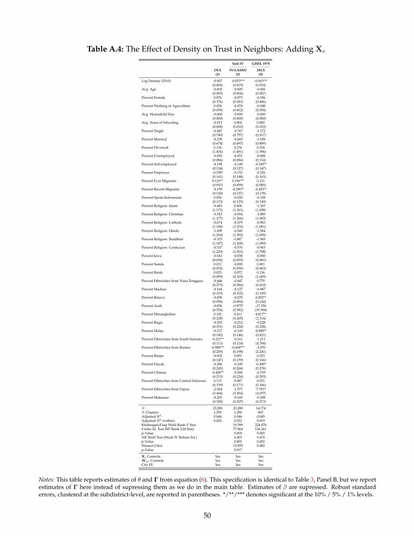
Table A.4: The Effect of Density on Trust in Neighbors: Adding Xv

Soil IV GHSL 1975

OLS IV-LASSO 2SLS(1) (2) (3)

Log Density (2010) -0.007 -0.053*** -0.043***(0.006) (0.019) (0.014)

Avg. Age -0.003 -0.005 -0.006(0.005) (0.006) (0.007)

Percent Female 0.076 -0.073 -0.186(0.376) (0.381) (0.406)

Percent Working in Agriculture 0.054 -0.074 -0.048(0.039) (0.062) (0.054)

Avg. Household Size -0.000 -0.000 -0.000(0.000) (0.000) (0.000)

Avg. Years of Schooling -0.013 0.002 0.002(0.008) (0.010) (0.010)

Percent Single -0.447 -0.767 -1.172(0.740) (0.757) (0.917)

Percent Married -0.239 -0.603 -1.038(0.674) (0.697) (0.809)

Percent Divorced 0.134 0.276 0.318(1.476) (1.491) (1.596)

Percent Unemployed -0.050 -0.051 -0.088(0.086) (0.086) (0.114)

Percent Self-employed -0.198 -0.149 -0.345**(0.124) (0.127) (0.147)

Percent Employer -0.238* -0.152 -0.226(0.141) (0.148) (0.163)

Percent Ever Migrants 0.123** 0.156*** 0.121(0.057) (0.059) (0.085)

Percent Recent Migrants -0.159 -0.290** -0.453**(0.120) (0.127) (0.178)

Percent Speak Indonesian 0.056 -0.020 -0.108(0.123) (0.125) (0.140)

Percent Religion: Islam -0.463 0.006 -1.107(1.172) (1.261) (1.058)

Percent Religion: Christian -0.523 -0.054 -1.089(1.177) (1.266) (1.065)

Percent Religion: Catholic -0.674 -0.379 -0.983(1.198) (1.270) (1.081)

Percent Religion: Hindu -1.009 -0.545 -1.584(1.200) (1.292) (1.095)

Percent Religion: Buddhist -0.333 0.087 -1.569(1.187) (1.268) (1.090)

Percent Religion: Confucian -0.537 -0.576 -0.903(1.229) (1.301) (1.708)

Percent Jawa -0.043 -0.038 -0.000(0.056) (0.055) (0.081)

Percent Sunda 0.012 -0.000 0.001(0.052) (0.050) (0.063)

Percent Batak 0.023 0.072 0.136(0.099) (0.103) (1.609)

Percent Ethnicities from Nusa Tenggara -0.446 -0.447 0.779(0.273) (0.284) (0.610)

Percent Madura -0.164 -0.127 -0.087(0.103) (0.102) (0.109)

Percent Betawi -0.090 -0.078 0.292**(0.096) (0.094) (0.144)

Percent Aceh -0.856 -0.975* -17.356(0.554) (0.582) (19.384)

Percent Minangkabau 0.182 0.411 4.817**(0.228) (0.265) (2.114)

Percent Bugis -0.255 -0.212 -0.228(0.191) (0.220) (0.228)

Percent Malay -0.217 -0.143 -0.880**(0.142) (0.146) (0.421)

Percent Ethnicities from South Sumatra -0.221** -0.161 -1.211(0.111) (0.114) (4.784)

Percent Ethnicities from Banten -0.580*** -0.604*** -3.470(0.205) (0.198) (2.241)

Percent Banjar -0.002 0.091 0.023(0.147) (0.159) (0.166)

Percent Dayak -0.280 -0.249 -0.490*(0.243) (0.266) (0.276)

Percent Chinese -0.436** -0.260 -0.159(0.215) (0.224) (0.293)

Percent Ethnicities from Central Sulawesi 0.115 0.087 0.031(0.159) (0.171) (0.166)

Percent Ethnicities from Papua -2.064 -1.571 -7.951*(3.404) (3.454) (4.077)

Percent Makassar -0.201 -0.165 -0.188(0.185) (0.207) (0.213)

N 23,280 23,280 14,774N Clusters 1,290 1,290 867Adjusted R2 0.044 0.046 0.045Adjusted R2 (within) 0.020 0.022 0.019Kleibergen-Paap Wald Rank F Stat 19.599 224.076Under Id. Test (KP Rank LM Stat) 77.864 126.261p-Value 0.000 0.000AR Wald Test (Weak IV Robust Inf.) 4.003 9.474p-Value 0.001 0.002Hansen J Stat 13.855 0.000p-Value 0.017

Xi Controls Yes Yes YesW2v Controls Yes Yes YesCity FE Yes Yes Yes

Notes: This table reports estimates of θ and Γ from equation (6). This specification is identical to Table 3, Panel B, but we reportestimates of Γ here instead of supressing them as we do in the main table. Estimates of β are supressed. Robust standarderrors, clustered at the subdistrict-level, are reported in parentheses. */**/*** denotes significant at the 10% / 5% / 1% levels.

50

Table A.5: The Effect of Density on Trust in Neighbors (Linear Index)

Soil IV GHSL 1975

OLS IV-LASSO 2SLS Dep.Var(1) (2) (3) Mean (SE) N

1. trust neighbor to watch house -0.028*** -0.056*** -0.048*** 2.916*** 23280.000(0.005) (0.012) (0.009) (0.003) (.)

... adding Xv controls -0.006 -0.059** -0.056***(0.009) (0.025) (0.020)

2. trust neighbor to tend children -0.053*** -0.078*** -0.057*** 2.649*** 23280.000(0.007) (0.016) (0.013) (0.004) (.)

... adding Xv controls -0.024** -0.062* -0.064**(0.011) (0.033) (0.026)

3. ready to help neighbor -0.000 0.010 -0.018** 2.978*** 23280.000(0.005) (0.012) (0.009) (0.003) (.)

... adding Xv controls 0.013 0.011 -0.030*(0.008) (0.024) (0.018)

4. contribute to assist unfortunate neigbhors -0.022*** -0.021 -0.045*** 2.808*** 23280.000(0.008) (0.016) (0.012) (0.005) (.)

... adding Xv controls -0.003 0.002 -0.043*(0.011) (0.033) (0.025)

5. easily access to neighbors’ help -0.026*** -0.034* -0.029** 2.649*** 23280.000(0.008) (0.017) (0.014) (0.005) (.)

... adding Xv controls 0.018 -0.001 0.051*(0.012) (0.036) (0.030)

City FE Yes Yes Yes

Notes: Each cell reports the coefficient on log population density in 2010 from a separate linear regression of (6) where thedependent variable is the outcome listed in the row header. Column 1 reports OLS estimates, while Column 2 applies a post-double-selection lasso estimator to select the best soil characteristics instruments, following Belloni et al. (2012). Columns 3use 2SLS with the GHSL 1975 instruments. In the first row of each panel, we only control for Xi and W2v , setting Γ1 = 0.The second row of each panel reports the full, unrestricted model. All regressions are limited to the sample of villages withinurban areas and include city-fixed effects. The sample size falls substantially in Column 3 because of missing GHSL 1975 datafor Sumatra. Robust standard errors, clustered at the subdistrict-level, are reported in parentheses. */**/*** denotes significantat the 10% / 5% / 1% levels.

51

Table A.6: The Effect of Density on Community Trust and Participation (Linear Index)

Soil IV GHSL 1975

OLS IV-LASSO 2SLS Dep.Var(1) (2) (3) Mean (SE) N

6. join community group(s) 0.014 -0.011 0.015 2.364*** 21767.000(0.009) (0.019) (0.016) (0.006) (.)

... adding Xv controls -0.007 -0.077* -0.097***(0.013) (0.041) (0.030)

7. join religious activities -0.035*** -0.044*** -0.045*** 2.683*** 22899.000(0.008) (0.015) (0.012) (0.005) (.)

... adding Xv controls -0.025** -0.035 -0.060**(0.011) (0.033) (0.027)

8. join religious activities recently -0.017*** -0.035*** -0.025*** 0.725*** 23006.000(0.004) (0.010) (0.008) (0.003) (.)

... adding Xv controls -0.016** -0.044** -0.036**(0.007) (0.021) (0.018)

9. voluntary public good provision -0.024*** -0.036* -0.038*** 2.503*** 22487.000(0.008) (0.018) (0.014) (0.005) (.)

... adding Xv controls -0.009 -0.046 -0.069**(0.013) (0.040) (0.029)

10. join community activities recently -0.008* -0.015* -0.010 0.796*** 22993.000(0.005) (0.009) (0.008) (0.003) (.)

... adding Xv controls -0.009 -0.030 -0.017(0.007) (0.019) (0.016)

11. trust religious leader -0.006 -0.012 -0.018** 3.051*** 23240.000(0.004) (0.009) (0.008) (0.003) (.)

... adding Xv controls 0.002 -0.005 -0.020(0.007) (0.020) (0.017)

12. trust communtiy leader -0.009** -0.016** -0.011 2.978*** 23280.000(0.004) (0.008) (0.007) (0.003) (.)

... adding Xv controls -0.003 -0.018 -0.011(0.006) (0.017) (0.015)

City FE Yes Yes Yes

Notes: Each cell reports the coefficient on log population density in 2010 from a separate linear regression of (6) where thedependent variable is the outcome listed in the row header. Column 1 reports OLS estimates, while Column 2 applies a post-double-selection lasso estimator to select the best soil characteristics instruments, following Belloni et al. (2012). Columns 3use 2SLS with the GHSL 1975 instruments. In the first row of each panel, we only control for Xi and W2v , setting Γ1 = 0.The second row of each panel reports the full, unrestricted model. All regressions are limited to the sample of villages withinurban areas and include city-fixed effects. The sample size falls substantially in Column 3 because of missing GHSL 1975 datafor Sumatra. Robust standard errors, clustered at the subdistrict-level, are reported in parentheses. */**/*** denotes significantat the 10% / 5% / 1% levels.

52

Table A.7: The Effect of Density on Intergroup Tolerance (Linear Index)

Soil IV GHSL 1975

OLS IV-LASSO 2SLS Dep.Var(1) (2) (3) Mean (SE) N

13. pleased with non-coreligions 0.046*** 0.038** 0.083*** 2.733*** 20578.000(0.009) (0.019) (0.017) (0.004) (.)

... adding Xv controls 0.040*** 0.012 0.059(0.013) (0.038) (0.037)

14. pleased with non-coethnics 0.015** -0.007 0.048*** 2.823*** 20742.000(0.007) (0.015) (0.014) (0.004) (.)

... adding Xv controls 0.015 -0.050 0.053*(0.011) (0.032) (0.031)

City FE Yes Yes Yes

Notes: Each cell reports the coefficient on log population density in 2010 from a separate linear regression of (6) where thedependent variable is the outcome listed in the row header. Column 1 reports OLS estimates, while Column 2 applies a post-double-selection lasso estimator to select the best soil characteristics instruments, following Belloni et al. (2012). Columns 3use 2SLS with the GHSL 1975 instruments. In the first row of each panel, we only control for Xi and W2v , setting Γ1 = 0.The second row of each panel reports the full, unrestricted model. All regressions are limited to the sample of villages withinurban areas and include city-fixed effects. The sample size falls substantially in Column 3 because of missing GHSL 1975 datafor Sumatra. Robust standard errors, clustered at the subdistrict-level, are reported in parentheses. */**/*** denotes significantat the 10% / 5% / 1% levels.

53

Table A.8: The Effect of Density on Trust in Neighbors (Linear Prob)

Soil IV GHSL 1975

OLS IV-LASSO 2SLS Dep.Var(1) (2) (3) Mean (SE) N

1. trust neighbor to watch house -0.020*** -0.038*** -0.034*** 0.843*** 23280.000(0.004) (0.009) (0.006) (0.002) (.)

... adding Xv controls -0.007 -0.053*** -0.043***(0.006) (0.019) (0.014)

2. trust neighbor to tend children -0.040*** -0.057*** -0.036*** 0.641*** 23280.000(0.006) (0.012) (0.010) (0.003) (.)

... adding Xv controls -0.023*** -0.059** -0.026(0.009) (0.027) (0.021)

3. ready to help neighbor -0.001 0.007 -0.008 0.880*** 23280.000(0.004) (0.008) (0.005) (0.002) (.)

... adding Xv controls 0.006 0.016 -0.002(0.005) (0.017) (0.012)

4. contribute to assist unfortunate neigbhors -0.018*** -0.017 -0.030*** 0.704*** 23280.000(0.005) (0.011) (0.008) (0.003) (.)

... adding Xv controls -0.010 -0.008 -0.031*(0.008) (0.023) (0.017)

5. easily access to neighbors’ help -0.019*** -0.022* -0.026*** 0.623*** 23280.000(0.006) (0.012) (0.010) (0.003) (.)

... adding Xv controls 0.006 -0.010 0.023(0.008) (0.026) (0.021)

City FE Yes Yes Yes

Notes: Each cell reports the coefficient on log population density in 2010 from a separate linear probability model of (6) wherethe dependent variable is a binary coarsening of the outcome listed in the row header. Column 1 reports OLS estimates, whileColumn 2 applies a post-double-selection lasso estimator to select the best soil characteristics instruments, following Belloniet al. (2012). Columns 3 use 2SLS with the GHSL 1975 instruments. In the first row of each panel, we only control for Xi andW2v , setting Γ1 = 0. The second row of each panel reports the full, unrestricted model. All regressions are limited to thesample of villages within urban areas and include city-fixed effects. The sample size falls substantially in Column 3 becauseof missing GHSL 1975 data for Sumatra. Robust standard errors, clustered at the subdistrict-level, are reported in parentheses.*/**/*** denotes significant at the 10% / 5% / 1% levels.

54

Table A.9: The Effect of Density on Community Trust and Participation (Linear Prob)

Soil IV GHSL 1975

OLS IV-LASSO 2SLS Dep.Var(1) (2) (3) Mean (SE) N

6. join community group(s) 0.006 -0.012 0.009 0.474*** 21767.000(0.005) (0.010) (0.009) (0.003) (.)

... adding Xv controls -0.006 -0.056** -0.039**(0.007) (0.024) (0.018)

7. join religious activities -0.021*** -0.022** -0.028*** 0.639*** 22899.000(0.005) (0.010) (0.008) (0.003) (.)

... adding Xv controls -0.021*** -0.022 -0.034*(0.007) (0.022) (0.018)

8. join religious activities recently -0.017*** -0.035*** -0.025*** 0.725*** 23006.000(0.004) (0.010) (0.008) (0.003) (.)

... adding Xv controls -0.018*** -0.046** -0.036*(0.007) (0.022) (0.018)

9. voluntary public good provision -0.019*** -0.024** -0.027*** 0.520*** 22487.000(0.005) (0.011) (0.009) (0.003) (.)

... adding Xv controls -0.020** -0.039 -0.049**(0.009) (0.026) (0.020)

10. join community activities recently -0.008* -0.015* -0.010 0.796*** 22993.000(0.005) (0.009) (0.008) (0.003) (.)

... adding Xv controls -0.012* -0.035* -0.018(0.007) (0.021) (0.018)

11. trust religious leader -0.003 -0.009** -0.006* 0.952*** 23240.000(0.002) (0.004) (0.003) (0.001) (.)

... adding Xv controls -0.000 -0.020** -0.006(0.003) (0.009) (0.007)

12. trust communtiy leader -0.008*** -0.013** -0.006 0.921*** 23280.000(0.003) (0.005) (0.004) (0.002) (.)

... adding Xv controls -0.006 -0.024** -0.002(0.004) (0.011) (0.010)

City FE Yes Yes Yes

Notes: Each cell reports the coefficient on log population density in 2010 from a separate linear probability model of (6) wherethe dependent variable is a binary coarsening of the outcome listed in the row header. Column 1 reports OLS estimates, whileColumn 2 applies a post-double-selection lasso estimator to select the best soil characteristics instruments, following Belloniet al. (2012). Columns 3 use 2SLS with the GHSL 1975 instruments. In the first row of each panel, we only control for Xi andW2v , setting Γ1 = 0. The second row of each panel reports the full, unrestricted model. All regressions are limited to thesample of villages within urban areas and include city-fixed effects. The sample size falls substantially in Column 3 becauseof missing GHSL 1975 data for Sumatra. Robust standard errors, clustered at the subdistrict-level, are reported in parentheses.*/**/*** denotes significant at the 10% / 5% / 1% levels.

55

Table A.10: The Effect of Density on Intergroup Tolerance (Linear Prob)

Soil IV GHSL 1975

OLS IV-LASSO 2SLS Dep.Var(1) (2) (3) Mean (SE) N

13. pleased with non-coreligions 0.034*** 0.032** 0.059*** 0.759*** 20578.000(0.007) (0.014) (0.012) (0.003) (.)

... adding Xv controls 0.028*** 0.004 0.038(0.010) (0.029) (0.027)

14. pleased with non-coethnics 0.011** -0.002 0.036*** 0.827*** 20742.000(0.005) (0.012) (0.011) (0.003) (.)

... adding Xv controls 0.010 -0.043* 0.044*(0.009) (0.026) (0.024)

City FE Yes Yes Yes

Notes: Each cell reports the coefficient on log population density in 2010 from a separate linear probability model of (6) wherethe dependent variable is a binary coarsening of the outcome listed in the row header. Column 1 reports OLS estimates, whileColumn 2 applies a post-double-selection lasso estimator to select the best soil characteristics instruments, following Belloniet al. (2012). Columns 3 use 2SLS with the GHSL 1975 instruments. In the first row of each panel, we only control for Xi andW2v , setting Γ1 = 0. The second row of each panel reports the full, unrestricted model. All regressions are limited to thesample of villages within urban areas and include city-fixed effects. The sample size falls substantially in Column 3 becauseof missing GHSL 1975 data for Sumatra. Robust standard errors, clustered at the subdistrict-level, are reported in parentheses.*/**/*** denotes significant at the 10% / 5% / 1% levels.

56

Table A.11: The Effect of Density on Trust in Neighbors (Binary Probit)

Soil IV GHSL 1975

ML ML ML Dep.Var(1) (2) (3) Mean (SE) N

1. trust neighbor to watch house -0.086*** -0.162*** -0.159*** 0.843*** 23280.000(0.017) (0.040) (0.029) (0.002) (.)

... adding X v controls -0.026 -0.237*** -0.212***(0.027) (0.092) (0.065)

2. trust neighbor to tend children -0.114*** -0.171*** -0.105*** 0.641*** 23280.000(0.016) (0.037) (0.029) (0.003) (.)

... adding X v controls -0.063** -0.201** -0.077(0.025) (0.086) (0.062)

3. ready to help neighbor -0.005 0.012 -0.048 0.880*** 23280.000(0.018) (0.041) (0.029) (0.002) (.)

... adding X v controls 0.027 0.031 -0.012(0.025) (0.090) (0.068)

4. contribute to assist unfortunate neigbhors -0.055*** -0.055 -0.095*** 0.704*** 23280.000(0.015) (0.034) (0.025) (0.003) (.)

... adding X v controls -0.031 -0.033 -0.101*(0.023) (0.072) (0.057)

5. easily access to neighbors’ help -0.052*** -0.060* -0.069*** 0.623*** 23280.000(0.015) (0.036) (0.026) (0.003) (.)

... adding X v controls 0.019 -0.039 0.069(0.022) (0.078) (0.059)

City FE Yes Yes Yes

Notes: Each cell reports the coefficient on log population density in 2010 from a separate binary probit model of (6). All columnsreport maximum likelihood estimates; column 1 reports them without using instruments, while columns 2 use the instrumentslisted in the column headers. In column 2, we follow Belloni et al. (2012) and use a lasso procedure to select the best soilcharacteristics instruments before implementing the ML estimator. In the first row of each panel, we only control for Xi andW2v , setting Γ1 = 0. The second row of each panel reports the full, unrestricted model. All regressions are limited to thesample of villages within urban areas and include city-fixed effects. The sample size falls substantially in Column 2 becauseof missing GHSL 1975 data for Sumatra. Robust standard errors, clustered at the subdistrict-level, are reported in parentheses.*/**/*** denotes significant at the 10% / 5% / 1% levels.

57

Table A.12: The Effect of Density on Community Trust and Participation (Binary Probit)

Soil IV GHSL 1975

ML ML ML Dep.Var(1) (2) (3) Mean (SE) N

6. join community group(s) 0.017 -0.054* 0.025 0.474*** 21767.000(0.013) (0.031) (0.025) (0.003) (.)

... adding X v controls -0.016 -0.187*** -0.114**(0.020) (0.072) (0.052)

7. join religious activities -0.060*** -0.063** -0.080*** 0.639*** 22899.000(0.013) (0.030) (0.023) (0.003) (.)

... adding X v controls -0.062*** -0.071 -0.100*(0.020) (0.068) (0.054)

8. join religious activities recently -0.055*** -0.093*** -0.080*** 0.725*** 23006.000(0.014) (0.034) (0.026) (0.003) (.)

... adding X v controls -0.058*** -0.110 -0.114*(0.022) (0.077) (0.062)

9. voluntary public good provision -0.052*** -0.061* -0.074*** 0.520*** 22487.000(0.014) (0.033) (0.024) (0.003) (.)

... adding X v controls -0.052** -0.104 -0.133**(0.024) (0.076) (0.055)

10. join community activities recently -0.032* -0.058 -0.038 0.796*** 22993.000(0.017) (0.037) (0.031) (0.003) (.)

... adding X v controls -0.046* -0.133 -0.069(0.026) (0.085) (0.071)

11. trust religious leader -0.026 -0.105** -0.075* 0.952*** 23240.000(0.021) (0.043) (0.040) (0.001) (.)

... adding X v controls -0.003 -0.255*** -0.089(0.031) (0.099) (0.086)

12. trust communtiy leader -0.049*** -0.087** -0.047 0.921*** 23280.000(0.017) (0.037) (0.033) (0.002) (.)

... adding X v controls -0.035 -0.176** -0.015(0.027) (0.083) (0.076)

City FE Yes Yes Yes

Notes: Each cell reports the coefficient on log population density in 2010 from a separate binary probit model of (6). All columnsreport maximum likelihood estimates; column 1 reports them without using instruments, while columns 2 use the instrumentslisted in the column headers. In column 2, we follow Belloni et al. (2012) and use a lasso procedure to select the best soilcharacteristics instruments before implementing the ML estimator. In the first row of each panel, we only control for Xi andW2v , setting Γ1 = 0. The second row of each panel reports the full, unrestricted model. All regressions are limited to thesample of villages within urban areas and include city-fixed effects. The sample size falls substantially in Column 2 becauseof missing GHSL 1975 data for Sumatra. Robust standard errors, clustered at the subdistrict-level, are reported in parentheses.*/**/*** denotes significant at the 10% / 5% / 1% levels.

58

Table A.13: The Effect of Density on Intergroup Tolerance (Binary Probit)

Soil IV GHSL 1975

ML ML ML Dep.Var(1) (2) (3) Mean (SE) N

13. pleased with non-coreligions 0.122*** 0.112** 0.196*** 0.759*** 20578.000(0.023) (0.052) (0.041) (0.003) (.)

... adding X v controls 0.102*** 0.009 0.126(0.036) (0.116) (0.092)

14. pleased with non-coethnics 0.051** -0.004 0.145*** 0.827*** 20742.000(0.022) (0.054) (0.040) (0.003) (.)

... adding X v controls 0.045 -0.160 0.186**(0.037) (0.129) (0.093)

City FE Yes Yes Yes

Notes: Each cell reports the coefficient on log population density in 2010 from a separate binary probit model of (6). All columnsreport maximum likelihood estimates; column 1 reports them without using instruments, while columns 2 use the instrumentslisted in the column headers. In column 2, we follow Belloni et al. (2012) and use a lasso procedure to select the best soilcharacteristics instruments before implementing the ML estimator. In the first row of each panel, we only control for Xi andW2v , setting Γ1 = 0. The second row of each panel reports the full, unrestricted model. All regressions are limited to thesample of villages within urban areas and include city-fixed effects. The sample size falls substantially in Column 2 becauseof missing GHSL 1975 data for Sumatra. Robust standard errors, clustered at the subdistrict-level, are reported in parentheses.*/**/*** denotes significant at the 10% / 5% / 1% levels.

59

Table A.14: The Effect of Density on Trust in Neighbors (Ordered Probit Using ControlFunction)

Soil IV GHSL 1975

ML CF CF Dep.Var(1) (2) (3) Mean (SE) N

1. trust neighbor to watch house -0.066*** -0.143*** -0.116*** 2.916*** 23280.000(0.013) (0.031) (0.022) (0.003) (.)

... adding X v controls -0.014 -0.187*** -0.138***(0.021) (0.065) (0.050)

2. trust neighbor to tend children -0.099*** -0.156*** -0.109*** 2.649*** 23280.000(0.014) (0.032) (0.024) (0.004) (.)

... adding X v controls -0.043** -0.154** -0.101*(0.021) (0.069) (0.054)

3. ready to help neighbor -0.001 0.014 -0.049** 2.978*** 23280.000(0.013) (0.031) (0.023) (0.003) (.)

... adding X v controls 0.033 0.027 -0.063(0.021) (0.067) (0.049)

4. contribute to assist unfortunate neigbhors -0.036*** -0.038 -0.073*** 2.808*** 23280.000(0.012) (0.028) (0.020) (0.005) (.)

... adding X v controls -0.010 -0.005 -0.064(0.019) (0.060) (0.042)

5. easily access to neighbors’ help -0.041*** -0.054* -0.044* 2.649*** 23280.000(0.013) (0.030) (0.022) (0.005) (.)

... adding X v controls 0.027 -0.025 0.065(0.019) (0.064) (0.051)

City FE Yes Yes Yes

Notes: Each cell reports the coefficient on log population density in 2010 from a separate ordered probit model of (6). Column1 reports maximum likelihood (ML) estimates, while columns 2-4 adopt the control function (CF) procedure described byChesher and Rosen (2019), together with the instruments listed in the column headers. In column 2, we follow Belloni et al.(2012) and use a lasso procedure to select the best soil characteristics instruments before implementing the control functionestimator. In the first row of each panel, we only control for Xi and W2v , setting Γ1 = 0. The second row of each panel reportsthe full, unrestricted model. All regressions are limited to the sample of villages within urban areas and include city-fixedeffects. The sample size falls substantially in Column 3 because of missing GHSL 1975 data for Sumatra. Robust standarderrors, clustered at the subdistrict-level, are reported in parentheses. */**/*** denotes significant at the 10% / 5% / 1% levels.

60

Table A.15: The Effect of Density on Community Trust and Participation (Ordered ProbitUsing Control Function)

Soil IV GHSL 1975

ML CF CF Dep.Var(1) (2) (3) Mean (SE) N

6. join community group(s) 0.018 -0.027 0.020 2.364*** 21767.000(0.011) (0.026) (0.020) (0.006) (.)

... adding X v controls -0.010 -0.113* -0.116***(0.017) (0.059) (0.041)

7. join religious activities -0.050*** -0.064*** -0.065*** 2.683*** 22899.000(0.011) (0.024) (0.018) (0.005) (.)

... adding X v controls -0.044** -0.060 -0.093**(0.017) (0.054) (0.042)

9. voluntary public good provision -0.033*** -0.047* -0.053*** 2.503*** 22487.000(0.012) (0.028) (0.020) (0.005) (.)

... adding X v controls -0.019 -0.060 -0.085*(0.019) (0.063) (0.044)

11. trust religious leader -0.021 -0.058* -0.060** 3.051*** 23240.000(0.015) (0.033) (0.026) (0.003) (.)

... adding X v controls 0.010 -0.071 -0.064(0.024) (0.074) (0.058)

12. trust communtiy leader -0.030** -0.065** -0.040 2.978*** 23280.000(0.014) (0.030) (0.025) (0.003) (.)

... adding X v controls -0.005 -0.081 -0.023(0.022) (0.067) (0.058)

City FE Yes Yes Yes

Notes: Each cell reports the coefficient on log population density in 2010 from a separate ordered probit model of (6). Column1 reports maximum likelihood (ML) estimates, while columns 2-4 adopt the control function (CF) procedure described byChesher and Rosen (2019), together with the instruments listed in the column headers. In column 2, we follow Belloni et al.(2012) and use a lasso procedure to select the best soil characteristics instruments before implementing the control functionestimator. In the first row of each panel, we only control for Xi and W2v , setting Γ1 = 0. The second row of each panel reportsthe full, unrestricted model. All regressions are limited to the sample of villages within urban areas and include city-fixedeffects. The sample size falls substantially in Column 3 because of missing GHSL 1975 data for Sumatra. Robust standarderrors, clustered at the subdistrict-level, are reported in parentheses. */**/*** denotes significant at the 10% / 5% / 1% levels.

61

Table A.16: The Effect of Density on Intergroup Tolerance (Ordered Probit Using ControlFunction)

Soil IV GHSL 1975

ML CF CF Dep.Var(1) (2) (3) Mean (SE) N

13. pleased with non-coreligions 0.100*** 0.082** 0.164*** 2.733*** 20578.000(0.019) (0.042) (0.034) (0.004) (.)

... adding X v controls 0.090*** 0.015 0.095(0.030) (0.087) (0.077)

14. pleased with non-coethnics 0.038** -0.021 0.118*** 2.823*** 20742.000(0.019) (0.040) (0.032) (0.004) (.)

... adding X v controls 0.038 -0.142 0.132*(0.030) (0.089) (0.074)

City FE Yes Yes Yes

Notes: Each cell reports the coefficient on log population density in 2010 from a separate ordered probit model of (6). Column1 reports maximum likelihood (ML) estimates, while columns 2-4 adopt the control function (CF) procedure described byChesher and Rosen (2019), together with the instruments listed in the column headers. In column 2, we follow Belloni et al.(2012) and use a lasso procedure to select the best soil characteristics instruments before implementing the control functionestimator. In the first row of each panel, we only control for Xi and W2v , setting Γ1 = 0. The second row of each panel reportsthe full, unrestricted model. All regressions are limited to the sample of villages within urban areas and include city-fixedeffects. The sample size falls substantially in Column 3 because of missing GHSL 1975 data for Sumatra. Robust standarderrors, clustered at the subdistrict-level, are reported in parentheses. */**/*** denotes significant at the 10% / 5% / 1% levels.

62

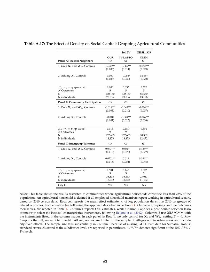
Table A.17: The Effect of Density on Social Capital: Dropping Agricultural Communities

Soil IV GHSL 1975

OLS IV-LASSO GMMPanel A: Trust in Neighbors (1) (2) (3)

1. Only Xi and W2v Controls -0.038*** -0.065*** -0.062***(0.006) (0.014) (0.009)

2. Adding Xv Controls 0.000 -0.052* -0.043**(0.008) (0.030) (0.020)

Ho : τ1 = τ2 (p-value) 0.000 0.655 0.322N Outcomes 5 5 5N 100,180 100,180 65,630N individuals 20,036 20,036 13,126

Panel B: Community Participation (1) (2) (3)

1. Only Xi and W2v Controls -0.018*** -0.045*** -0.034***(0.005) (0.010) (0.007)

2. Adding Xv Controls -0.010 -0.069*** -0.046***(0.007) (0.023) (0.016)

Ho : τ1 = τ2 (p-value) 0.113 0.189 0.394N Outcomes 9 9 9N 137,605 137,605 90,309N individuals 18,873 18,873 12,472

Panel C: Intergroup Tolerance (1) (2) (3)

1. Only Xi and W2v Controls 0.077*** 0.050* 0.135***(0.012) (0.027) (0.022)

2. Adding Xv Controls 0.072*** 0.011 0.144***(0.018) (0.054) (0.046)

Ho : τ1 = τ2 (p-value) 0.581 0.145 0.607N Outcomes 5 5 5N 36,133 36,133 23,017N individuals 18,012 18,012 11,472

City FE Yes Yes Yes

Notes: This table shows the results restricted to communities where agricultural households constitute less than 25% of thepopulation. An agricultural household is defined if all employed household members report working in agricultural sectors,based on 2010 census data. Each cell reports the mean effect estimate, τ , of log population density in 2010 on groups ofrelated outcomes, from equation (4), following the approach described in Section 5.4. Outcome groupings, and the outcomesthemselves, are repoted in Table 1. Column 1 reports OLS estimates, while Column 2 applies a post-double-selection lassoestimator to select the best soil characteristics instruments, following Belloni et al. (2012). Columns 3 use 2SLS/GMM withthe instruments listed in the column header. In each panel, in Row 1, we only control for Xi and W2v , setting Γ = 0. Row3 reports the full, unrestricted model. All regressions are limited to the sample of villages within urban areas and includecity-fixed effects. The sample size falls substantially in Column 3 because of missing GHSL 1975 data for Sumatra. Robuststandard errors, clustered at the subdistrict-level, are reported in parentheses. */**/*** denotes significant at the 10% / 5% /1% levels.

63

Table A.18: The Effect of Density on Social Capital: Mean Effects, Adding More Controls

Soil IV GHSL 1975

OLS IV-LASSO 2SLSPanel A: Trust in Neighbors (1) (2) (3)

1. Only Xi and W2v Controls -0.041*** -0.064*** -0.064***(0.005) (0.011) (0.008)

2. Adding Xv Controls -0.002 -0.058** -0.048***(0.008) (0.024) (0.018)

3. Adding More W2v Controls -0.002 -0.063** -0.036*(0.008) (0.025) (0.020)

Panel B: Community Participation (1) (2) (3)

1. Only Xi and W2v Controls -0.022*** -0.047*** -0.035***(0.004) (0.009) (0.007)

2. Adding Xv Controls -0.019*** -0.075*** -0.063***(0.006) (0.019) (0.015)

3. Adding More W2v Controls -0.017*** -0.076*** -0.057***(0.006) (0.020) (0.016)

Panel C: Intergroup Tolerance (1) (2) (3)

1. Only Xi and W2v Controls 0.054*** 0.030 0.118***(0.010) (0.021) (0.020)

2. Adding Xv Controls 0.046*** -0.031 0.100**(0.016) (0.046) (0.045)

3. Adding More W2v Controls 0.046*** -0.047 0.122**(0.017) (0.048) (0.048)

City FE Yes Yes Yes

Notes: Each cell reports the mean effect estimate, τ , of log population density in 2010 on groups of related outcomes, fromequation (4), following the approach described in Section 5.4. Outcome groupings, and the outcomes themselves, are repotedin Table 1. Column 1 reports OLS estimates, while Column 2 applies a post-double-selection lasso estimator to select the bestsoil characteristics instruments, following Belloni et al. (2012). Columns 3 use 2SLS with the GHSL 1975 instruments. In eachpanel, in Row 1, we only control for Xi and W2v , setting Γ1 = 0. Row 2 reports the full, unrestricted model. All regressions arelimited to the sample of villages within urban areas and include city-fixed effects. The sample size falls substantially in Column3 because of missing GHSL 1975 data for Sumatra. Robust standard errors, clustered at the subdistrict-level, are reported inparentheses. */**/*** denotes significant at the 10% / 5% / 1% levels. The additional W2v include the community’s distanceto formal markets, if any restaurants exist, distance to schools, if there are any mobile phone or TV signals, the type of mainwater sources, if there are local community empowerment programs, the number of houses of worships, distance to medicalfacilities, and distance to maternal health facilities.

64

Table A.19: Summary Statistics: Social Capital Outcomes (IFLS 5)

Panel A: Trust in Neighbors Description Code Mean (sd) N

Trust neighbors to return wallet Would you trust your neighbors to return your wallet if it was lost? TR08 2.87 (1.05) 15,964Trust neighbor to watch house I would ask my neighbors to watch my house if I leave for a few days. TR05 2.81 (0.57) 16,326Trust neighbor to tend to children I would leave children w/ neighbors for a few hours if I can’t bring them along. TR04 2.56 (0.64) 11,656Willing to help villagers in need I am willing to help people in this village if they need it. TR01 3.24 (0.46) 16,326

Panel B: Community Trust and Participation Description Code Mean (sd) N

Participate in village meetings? In the last 12 months, did you participate in any village meetings? PM16A 0.21 (0.41) 16,219Participate in cooperatives? In the last 12 months, did you participate in any cooperative? PM16B 0.04 (0.19) 16,219Participate in voluntary labor? In the last 12 months, did you participate in any voluntary labor? PM16C 0.27 (0.44) 16,219Participate in program to improve the neighborhood? In the last 12 months, did you participate in any program to improve the neighborhood? PM16D 0.20 (0.40) 16,219Participate in youth group activities? In the last 12 months, did you participate in any youth group activities (Karang Taruna)? PM16E 0.08 (0.27) 16,219Participate in religious activities? In the last 12 months, did you participate in any religious activities (Prayer groups, etc.)? PM16F 0.52 (0.50) 16,219

Panel C: Intergroup Tolerance Description Code Mean (sd) N

Trust own ethnic group more Do you trust people with the same ethnicity as mine more than others TR03 2.30 (0.66) 16,326Trust own religious group more Do you trust people with the same relgion as mine more than others TR23 2.04 (0.67) 16,325Tolerate diff. faith living in the same village What if someone with a different faith lives in your village? TR24 2.82 (0.59) 16,326Tolerate diff. faith living in the same neighborhood What if someone with a different faith lives in your neighborhood? TR25 2.81 (0.58) 16,326Tolerate diff. faith renting a room What if someone with a different faith rents a room from you? TR26 2.46 (0.71) 16,326Tolerate diff. faith marrying relatives What if someone with a different faith marries a close relative or child? TR27 1.78 (0.72) 16,325Tolerate diff. faith building house of worship nearby What if people with a different faith build a house of worship in your community? TR28 2.27 (0.77) 16,326

Notes: This table reports short titles, longer descriptions, and summary statistics for the social capital outcomes we analyze from the IFLS 5 data (2014-2015). Summarystatistics were computed using data only from the sample of communities comprising metropolitan areas. The groupings of variables listed here correspond to the groupingsused in the IFLS 5 mean effects analysis (e.g. Table 5).

65

Table A.20: Summary Statistics: Social Capital Outcomes (IFLS 4)

Panel A: Trust in Neighbors Description Code Mean (sd) N

Trust neighbors to return wallet Would you trust your neighbors to return your wallet if it was lost? TR08 2.99 (0.94) 13,784Trust neighbor to watch house I would ask my neighbors to watch my house if I leave for a few days. TR05 2.84 (0.47) 14,092Trust neighbor to tend to children I would leave children w/ neighbors for a few hours if I can’t bring them along. TR04 2.61 (0.58) 10,459Willing to help villagers in need I am willing to help people in this village if they need it. TR01 3.14 (0.37) 14,094

Panel B: Community Trust and Participation Description Code Mean (sd) N

Participate in village meetings? In the last 12 months, did you participate in any village meetings? PM16A 0.21 (0.41) 14,085Participate in cooperatives? In the last 12 months, did you participate in any cooperative? PM16B 0.03 (0.16) 14,085Participate in voluntary labor? In the last 12 months, did you participate in any voluntary labor? PM16C 0.26 (0.44) 14,085Participate in program to improve the neighborhood? In the last 12 months, did you participate in any program to improve the neighborhood? PM16D 0.18 (0.38) 14,085Participate in youth group activities? In the last 12 months, did you participate in any youth group activities (Karang Taruna)? PM16E 0.06 (0.23) 14,085Participate in religious activities? In the last 12 months, did you participate in any religious activities (Prayer groups, etc.)? PM16F 0.50 (0.50) 14,085

Panel C: Intergroup Tolerance Description Code Mean (sd) N

Trust own ethnic group more Do you trust people with the same ethnicity as mine more than others TR03 2.41 (0.58) 14,093Trust own religious group more Do you trust people with the same relgion as mine more than others TR23 2.26 (0.58) 14,094Tolerate diff. faith living in the same village What if someone with a different faith lives in your village? TR24 2.86 (0.48) 14,094Tolerate diff. faith living in the same neighborhood What if someone with a different faith lives in your neighborhood? TR25 2.83 (0.51) 14,094Tolerate diff. faith renting a room What if someone with a different faith rents a room from you? TR26 2.50 (0.68) 14,093Tolerate diff. faith marrying relatives What if someone with a different faith marries a close relative or child? TR27 1.75 (0.79) 14,093Tolerate diff. faith building house of worship nearby What if people with a different faith build a house of worship in your community? TR28 2.33 (0.78) 14,094

Notes: This table reports short titles, longer descriptions, and summary statistics for the social capital outcomes we analyze from the IFLS 4 data (2007). Summary statisticswere computed using data only from the sample of communities comprising metropolitan areas. The groupings of variables listed here correspond to the groupings used inthe IFLS 4 mean effects analysis (e.g. Appendix Table A.21).

66

Table A.21: The Effect of Density on Social Capital: Mean Effects (IFLS 4)

Soil IV GHSL 1975

OLS IV-LASSO 2SLSPanel A: Trust in Neighbors (1) (2) (3)

1. Only Xi and W2v Controls -0.043*** -0.067*** -0.081***(0.007) (0.014) (0.015)

2. Adding Xv Controls -0.014 -0.099** -0.079(0.009) (0.042) (0.059)

N 53,917 53,898 31,305N individuals 14,474 14,469 8,366N Outcomes 4 4 4Ho : Γ = 0 (p-value) 0.000 0.000 0.000Ho : τ1 = τ2 (p-value) 0.000 0.674 0.998

Panel B: Community Participation (1) (2) (3)

1. Only Xi and W2v Controls -0.029*** -0.014 -0.055***(0.006) (0.012) (0.014)

2. Adding Xv Controls -0.018** 0.049 -0.042(0.007) (0.031) (0.052)

N 86,802 86,772 50,214N individuals 14,467 14,462 8,369N Outcomes 6 6 6Ho : Γ = 0 (p-value) 0.000 0.000 0.000Ho : τ1 = τ2 (p-value) 0.020 0.002 0.583

Panel C: Intergroup Tolerance (1) (2) (3)

1. Only Xi and W2v Controls 0.088*** 0.120*** 0.082***(0.007) (0.013) (0.012)

2. Adding Xv Controls 0.043*** 0.170*** 0.070(0.008) (0.035) (0.044)

N 101,316 101,281 58,560N individuals 14,474 14,469 8,366N Outcomes 7 7 7Ho : Γ = 0 (p-value) 0.000 0.000 0.000Ho : τ1 = τ2 (p-value) 0.000 0.196 0.931

City FE Yes Yes Yes

Notes: Each cell reports the mean effect estimate, τ , of log population density in 2010 on groups of related outcomes, fromequation (4), following the approach described in Section 5.4, but using the IFLS 4 data for outcomes. Outcome groupings,and the outcomes themselves, are repoted in Appendix Table A.20. Column 1 reports OLS estimates, while Column 2 applies apost-double-selection lasso estimator to select the best soil characteristics instruments, following Belloni et al. (2012). Columns3 use 2SLS with the GHSL 1975 instruments. In each panel, in Row 1, we only control for Xi and W2v , setting Γ1 = 0. Row2 reports the full, unrestricted model. All regressions are limited to the sample of villages within urban areas and includecity-fixed effects. The sample size falls substantially in Column 3 because of missing GHSL 1975 data for Sumatra. Robuststandard errors, clustered at the subdistrict-level, are reported in parentheses. */**/*** denotes significant at the 10% / 5% /1% levels.

67

Table A.22: Mean Effects, IFLS Panel Regressions (Single Index First Step)

Soil IV GHSL 1975

OLS IV-LASSO 2SLS(1) (2) (3)

Trust in neighbors -0.096** -0.201*** 0.023(0.045) (0.073) (0.129)

N 174 173 91Adjusted R2 0.016 -0.016 -0.016Kleibergen-Paap Wald Rank F Stat 36.885 28.097Under Id. Test (KP Rank LM Stat) 42.291 24.556p-Value 0.000 0.000AR Wald Test (Weak IV Robust Inf.) 3.266 0.031p-Value 0.013 0.860

Community participation -0.038 -0.045 -0.024(0.038) (0.064) (0.085)

N 174 173 91Adjusted R2 -0.001 -0.009 -0.009Kleibergen-Paap Wald Rank F Stat 36.885 28.097Under Id. Test (KP Rank LM Stat) 42.291 24.556p-Value 0.000 0.000AR Wald Test (Weak IV Robust Inf.) 1.599 0.080p-Value 0.177 0.778

Intergroup tolerance 0.091** 0.129* 0.023(0.041) (0.074) (0.061)

N 174 173 91Adjusted R2 0.024 0.020 -0.015Kleibergen-Paap Wald Rank F Stat 36.885 28.097Under Id. Test (KP Rank LM Stat) 42.291 24.556p-Value 0.000 0.000AR Wald Test (Weak IV Robust Inf.) 1.496 0.141p-Value 0.206 0.708

Notes: This table reports panel regression results using IFLS 4/5 data. A single index is created by taking average over allrelated outcome variables seperately for each group. Then the 3 constructed single-index outcomes variables, namely trust inneighbors, community participation and Intergroup tolerance are regressed on log density. Column 1 reports OLS estimates,while Column 2 applies a post-double-selection lasso estimator to select the best soil characteristics instruments, followingBelloni et al. (2012). Columns 3 use 2SLS with the GHSL 1975 instruments. In each panel, in Row 1, we only control for Xi andW2v , setting Γ1 = 0. Row 2 reports the full, unrestricted model. All regressions are limited to the sample of villages withinurban areas and include city-fixed effects. The sample size falls substantially in Column 3 because of missing GHSL 1975 datafor Sumatra. Robust standard errors, clustered at the subdistrict-level, are reported in parentheses. */**/*** denotes significantat the 10% / 5% / 1% levels. Robust standard errors, clustered at the subdistrict-level, are reported in parentheses. */**/***denotes significant at the 10% / 5% / 1% levels.

68

Table A.23: Heterogeneous Effects of Density on Social Capital: Individual-Level Interac-tions (Soil IV)

Panel A: Trust in Neighbors (1) (2) (3) (4) (5) (6)

Log density -0.058** -0.055** -0.052** -0.027 -0.053* -0.050**(0.02) (0.02) (0.02) (0.02) (0.03) (0.02)

. . . × Age: 41-65 -0.049**(0.02)

. . . × Age: +65 -0.059**(0.03)

. . . ×Married -0.050**(0.02)

. . . × Education: High -0.056**(0.02)

. . . × Income: Middle -0.044*(0.02)

. . . × Income: High -0.058**(0.03)

. . . × Private -0.080***(0.03)

Panel B: Community Trust and Participation (1) (2) (3) (4) (5) (6)

Log density -0.075*** -0.087*** -0.079*** -0.059*** -0.057*** -0.053***(0.019) (0.019) (0.019) (0.019) (0.022) (0.020)

. . . × Age: 41-65 -0.074***(0.018)

. . . × Age: +65 -0.055***(0.020)

. . . ×Married -0.082***(0.019)

. . . × Education: High -0.080***(0.019)

. . . × Income: Middle -0.058***(0.019)

. . . × Income: High -0.068***(0.020)

. . . × Private -0.076***(0.021)

Panel C: Intergroup Tolerance (1) (2) (3) (4) (5) (6)

Log density -0.031 -0.041 -0.080* -0.052 -0.110** -0.045(0.046) (0.044) (0.044) (0.046) (0.054) (0.050)

. . . × Age: 41-65 -0.043(0.045)

. . . × Age: +65 -0.059(0.048)

. . . ×Married -0.067(0.044)

. . . × Education: High -0.045(0.043)

. . . × Income: Middle -0.074(0.046)

. . . × Income: High -0.036(0.044)

. . . × Private -0.050(0.048)

Notes: This table reports mean effects and mean interaction terms for the impact of density on social capital, using soil qual-ity variables and their interactions as instruments and including both the W2v and Xv controls. For each panel, Column 1replicates estimates from Table 4, Column 2, Row 3. See Appendix B.5 for more details on the estimation methodology andvariables used for Columns 2-4. Robust standard errors, clustered at the subdistrict-level, are reported in parentheses. */**/***denotes significant at the 10% / 5% / 1% levels.

69

Table A.24: Heterogeneous Effects of Density on Social Capital: City-Level Interactions(Soil IV)

Panel A: Trust in Neighbors (1) (2) (3) (4) (5) (6)

Log density -0.058** -0.034 -0.056** -0.060** -0.030 -0.051*(0.02) (0.03) (0.03) (0.03) (0.03) (0.03)

. . . × Urban core: Large -0.046*(0.02)

. . . × Sprawl (2000-2014): High -0.051**(0.02)

. . . × Ethinic Frac: High -0.042*(0.02)

. . . × Property Crime: High -0.069***(0.02)

. . . × Violent Crime: High -0.031(0.02)

Panel B: Community Trust and Participation (1) (2) (3) (4) (5) (6)

Log density -0.075*** -0.065*** -0.061*** -0.085*** -0.065*** -0.076***(0.019) (0.021) (0.020) (0.024) (0.019) (0.021)

. . . × Urban core: Large -0.052***(0.019)

. . . × Sprawl (2000-2014): High -0.054***(0.018)

. . . × Ethinic Frac: High -0.062***(0.018)

. . . × Property Crime: High -0.087***(0.019)

. . . × Violent Crime: High -0.075***(0.018)

Panel C: Intergroup Tolerance (1) (2) (3) (4) (5) (6)

Log density -0.031 -0.050 -0.026 -0.022 -0.026 -0.096*(0.046) (0.042) (0.050) (0.070) (0.049) (0.057)

. . . × Urban core: Large -0.054(0.048)

. . . × Sprawl (2000-2014): High -0.023(0.046)

. . . × Ethinic Frac: High -0.024(0.042)

. . . × Property Crime: High -0.053(0.049)

. . . × Violent Crime: High -0.032(0.044)

Notes: This table reports mean effects and mean interaction terms for the impact of density on social capital, using soil qual-ity variables and their interactions as instruments and including both the W2v and Xv controls. For each panel, Column 1replicates estimates from Table 4, Column 2, Row 3. See Appendix B.5 for more details on the estimation methodology andvariables used for Columns 2-4. Robust standard errors, clustered at the subdistrict-level, are reported in parentheses. */**/***denotes significant at the 10% / 5% / 1% levels.

70

Table A.25: The Effect of Density on Trust: Model Regressions to Control for Sorting

Dep Var: realized p0 Dep Var: realized p1 Dep Var: r0 Dep Var: r1 Dep Var: Πinv Dep Var: Πtru

(1) (2) (3) (4) (5) (6) (7) (8) (9) (10) (11) (12)

Q (Density−1) 0.762*** 1.372*** 0.660*** 2.367*** 0.214*** 0.652*** 0.107*** 0.457*** 0.155*** 0.404*** 1.671*** 5.316***(0.005) (0.027) (0.002) (0.013) (0.007) (0.012) (0.003) (0.008) (0.006) (0.012) (0.005) (0.031)

Q2 (Density−1) -0.610*** -1.707*** -0.437*** -0.349*** -0.249*** -3.645***(0.027) (0.012) (0.013) (0.005) (0.008) (0.028)

α (Group Share) -0.447*** -0.447*** 0.037*** 0.037*** -0.094*** -0.094*** -0.022*** -0.022*** -0.113*** -0.113*** 1.086*** 1.086***(0.027) (0.027) (0.006) (0.006) (0.016) (0.016) (0.005) (0.005) (0.010) (0.010) (0.016) (0.016)

R (Intolerant Share) -1.027*** -1.027*** 0.029** 0.029** -0.232*** -0.232*** -0.013 -0.013 -0.047** -0.047** -0.583*** -0.583***(0.026) (0.026) (0.010) (0.010) (0.025) (0.025) (0.008) (0.008) (0.018) (0.018) (0.034) (0.034)

N 8,400 8,400 8,400 8,400 8,400 8,400 8,400 8,400 8,400 8,400 8,400 8,400N Clusters 20 20 20 20 20 20 20 20 20 20 20 20Adjusted R2 0.841 0.871 0.588 0.875 0.499 0.623 0.373 0.653 0.649 0.752 0.682 0.895

Simulation FE Yes Yes Yes Yes Yes Yes Yes Yes Yes Yes Yes Yes

Notes: This table reports the effect of density on trust using the simulated data. Column (1), (3), (5), (7), (9), and (11) reports the linear specication results for outsomes shownin the header, while (2), (4), (6), (8), (10), and (12) reports the quadratic specication results. All regressions include simulation-fixed effects. Standard errors are clustered atthe simulation-level, are reported in parentheses. */**/*** denotes significant at the 10% / 5% / 1% levels.

71

Figure A.1: GHSL 1975: Built Up Area

Notes: This figure plots the built up extent of villages in Indonesia using the GHSL 1975 data. Locations with a larger percentageof built up areas are shaded in darker blue. The red portions of this figure indicate areas where the 1975 data are missing. Thefigure assigns each village to the average of the GHSL 1975 raster for that village, using the 2010 village shapefile from BPS.

Figure A.2: Urban Sprawl vs. Population of the Urban Core Area in 2000

Notes: This figure presents a scatterplot of the relationship between urban sprawl (from 2000-2014) and the population of theurban core area of each city in 2000. The estimated semi-elasticity of the linear regression line is −1.02 (p-value .00). Each pointin the scatterplot represents a different city. The horizontal axis is expressed in log-scale.

72

Figure A.3: Bandar Lampung Core and Fringe Identification

(A) FROM BUILT-UP TO THE CORE (B) ADDING THE FRINGE

Notes: This figure illustrates the procedure we follow to identify core and fringe of a metropolitan area from the built-upraster data. We use the metropolitan region corresponding to the city of Bandar Lampung as an example. Panel A reportsthe pixels in the map covered by built-up in 2000 (light blue) and those corresponding to new built-up by 2014 (dark violet).The light green polygon in the background depicts the Southern tip of Sumatra. The pixels of 2000 built-up areas identifiedas core by Burchfield et al. (2006) methodology are indicated in dark blue. For this city, a major core is visible at the center ofthe map, while a second smaller satellite core can be seen moving South-East along the shore. Panel B simply adds the fringeconstructed around this core (in orange). The fringe is obtained as a 20km buffer around the core, which is then intersected withboundaries of the administrative units belonging to this metropolitan area. Bandar Lampung comprises two administrativeregions, as described in Appendix Figure A.4.

73

Figure A.4: Bandar Lampung Core-Fringe and Administrative Boundaries

(A) CORE VS. ADMIN. UNITS (B) METRO AREA AND ADMIN. BOUNDARIES

Notes: This figure is a continuation of Appendix Figure A.3 and illustrates how the metropolitan area identified by the Burch-field et al. (2006) methodology compares to the boundaries of the administrative units corresponding to it. The metropolitanarea encompasses two administrative regions, which can be seen in Panel A. The dark green unit is the city (kota) of BandarLampung, while the crimson unit is the district (kabupaten) of Lampung Selatan. The core of the metropolitan area from FigureA.3 is also reported in dark blue. It is important to observe that the main portion of the core does not overlap with the adminis-trative boundaries of the kota, being actually smaller, while the secondary part completely lies within the kabupaten. In Panel B,the identified metropolitan area is superimposed onto the administrative definition of it. The figure shows that the identifiedmetropolitan area is also smaller than the simple union of the two administrative units. Moreover, it is evident that the area isdelimited by the administrative boundaries when the radius of the fringe exceeds those boundaries.

74

B Empirical Strategy Appendix

B.1 An IV Estimator for θ

Recall that Xiv ≡ [Xi,Xv,W2v] collects observed variables that do not include density. An IV estimator for (θ, β)

solves the following two moment equations:

0 = Z′(y − θIV log density− XβIV )

0 = X′(y − θIV log density− XβIV ).

The second equation can be used to solve for βIV as follows:

βIV =

(X′X

)−1X′(y − θIV log density

).

Plugging this expression into the first equation gives us the following expression for the IV estimator of θ, ourparameter of interest:

θIV =(Z′MXlog density

)−1Z′MXy

where MX =

(I− X

(X′X

)−1X′)

is the standard orthogonal projection matrix for X.

B.2 Bias of θIV

An expression for the bias of θIV is the following:

Bias(θIV

)= E

[θIV

]− θ

= E[(

Z′MXlog density)−1

Z′MXy]− θ

= E[(

Z′MXlog density)−1

Z′MX E[y

∣∣∣∣ Z, X, log density]]− θ

= E[(

Z′MXlog density)−1

Z′MX

(θ log densityv + Xivβ + E

[uiv

∣∣∣∣ Z, X, log density])]

− θ

= θ + 0 + E[(

Z′MXlog density)−1

Z′MX E[uiv

∣∣∣∣ Z, X, log density]]− θ

= E[(

Z′MXlog density)−1

Z′MX E[uiv

∣∣∣∣ Z, X, log density]]

= E

(Z′MXlog density)−1

Z′MX E

xUi︸︷︷︸(A)

+ wUv︸︷︷︸(B)

+ ηvi︸︷︷︸(C)

+ ξvi︸︷︷︸(D)

∣∣∣∣ Z, X, log density

This bias expression contains four terms, which we describe separately. For term (A), the sorting model describedby Altonji and Mansfield (2018), together with their assumptions A1-A5, delivers their proposition 1, which isnamely that the expectation of xUv is linearly dependent on Xv , the group-level observables. This means that wehave the following:

(A) : E[(

Z′MXlog density)−1

Z′MXE[xUi

∣∣∣∣ Z, X, log density]]

= 0

since the expectation of xUi is in the space spanned by the columns of X.For term (C), note that W2v is defined as a vector of village-level characteristics not mechanically related to

75

sorting, so W2v is uncorrelated with ηvi by definition. Hence, we can write:

ηvi = XiPXi+ e

where PXiis a projection matrix and e is the orthogonal component, which is mean zero given X.49 This means

that ηvi is in the space spanned by the columns of X and hence term (C) is zero:

(C) : E[(

Z′MXlog density)−1

Z′MXE[ηvi

∣∣∣∣ Z, X, log density]]

= 0

For term (D), we assumed that ξvi was unpredictable given all unobservables in the model, so that by con-struction, we have:

(D) : E[ξvi

∣∣∣∣ Z, X, log density]

= 0.

So, we are left with the following expression for the bias in θIV :

Bias(θIV

)= E

[(Z′MXlog density

)−1Z′MX E

[wUv

∣∣∣∣ Z, X, log density]]

So, in order for our IV to be unbiased, a sufficient condition is that conditional on Z and the other observedindividual and village-level variables, wUv is mean zero.

E[wUv

∣∣∣∣ Z, X, log density]

= 0

What this amounts to is that our density shifters, namely soil quality of the village or lagged population measures,need to be uncorrelated with unobservables that influence overall village-level social capital. We discuss theplausibility of this assumption in the main text of the paper.

B.3 Mean Effects Analysis

Our estimate of the mean effects of density on groups of related outcomes is based on the procedure in Klinget al. (2007) (see footnote 22). Let k = 1, ...,K index outcome variables for a group of related outcomes (e.g. trustin neighbors, inter-ethnic tolerance, etc.). Let Y = [y′1,y

′2, ...,y

′K ]′ denote a stacked vector of K social capital

outcomes for that group. Let X be denoted as follows:

X =

X1 0 ... 0

0 X2 ... 0...

.... . .

...0 0 ... XK

where Xk consists of the control variables for outcome k. In our initial regression, this will only include

individual-specific controls Xi, predetermined community characteristics W2v and the city-specific intercepts,but later regressions will add Xv. Also stack the independent variables as follows:

D =

log density 0 ... 0

0 log density ... 0...

.... . .

...0 0 ... log density

49This is equation (11) in Altonji and Mansfield (2018).

76

After stacking and appropriately arranging the variables, we can estimate mean effects using the following singleregression:

Y = Xβ + Dθ + ε (13)

With OLS, this is straightforward, but with IVs, we need to use an appropriately stacked vector:

Z =

Z1 0 ... 0

0 Z2 ... 0...

.... . .

...0 0 ... ZK

After estimating the parameters of this regression (with OLS or IV), we obtain the mean effect estimate as follows:

τ =1

K

K∑k=1

θkσk

where σk is the standard deviation of yk. We ignore sampling variation in σk when estimating τ .

B.4 IFLS Panel Specification (SUR System)

Another approach to dealing with sorting is to use a two-step estimator (Combes et al., 2010). In the first step,we estimate local fixed effects of social capital, which condition out the impact of individual-specific effects andthe effect of time-varying individual-level observables. We then average the residuals from this regression, andestimate a cross-sectional regression of the average social capital measures (averaged over village years) on ourdensity measure in 2010.

Let k = 1, ...,K denote a group of related social capital outcomes, and let Y kit : social capital outcome k forindividual i at time t. The vector xit consists of time-varying individual-level characteristics for individual i, suchas that individual’s educational attainment at time t, their marital status at time t, age at time t, and householdsize at time t. We first stack the outcome variables in a vector, Y = [y′1,y

′2, ...,y

′K ]′. Let X be denoted as follows:

X =

X1 0 ... 0

0 X2 ... 0...

.... . .

...0 0 ... XK

where Xk consists of the control variables for outcome k (e.g. the time-varying individual-level controls). Let D

be a matrix individual fixed effects for outcome k (i.e. di), specific to each individual and outcome:

D =

D1 0 ... 0

0 D2 ... 0...

.... . .

...0 0 ... DK

Let A = [αjt] denote a row vector of effects for each village and year (e.g. the αjt’s). This is common to alloutcomes.

In the first step of the (Combes et al., 2010) estimator, we estimate αjt for all equations using a SUR system:

Y = Xβ + Dθ + A + ε (14)

77

The A vector will contain the αjt estimates, which are estimates of the social capital index for each village andyear, after conditioning out individual fixed effects and time-varying individual-level observables.50

Next, in the second step, we form the cross-sectional average of these village-year fixed effects:

αj =1

T

T∑t=1

αjt

We then use αj as the independent variable in the following regression:

αj = W2vβ2 + θ log densityv + ∆εi

where we instrument log densityv with our 2 sets of instruments.

B.5 Heterogeneous Effects (SUR System)

To estimate heterogeneous effects of density, we add a matrix of levels terms,

M =

M1 0 ... 0

0 M2 ... 0...

.... . .

...0 0 ... MK

where MK consists of the level variables for outcome k, and a stacked vector of interaction terms with density,

N ≡M ·D =

M1 ·D1 0 ... 0

0 M2 ·D2 ... 0...

.... . .

...0 0 ... MK ·DK

to (13), and we estimate the following regression using our instrument set which is augmented by interactionsbetween M and the original instruments:

Y = Xβ + Mγ + Dθ + Nθ1 + ε (15)

Then we obtain the mean effect estimates for the reference group, τ , and for the interaction terms, τ1, asfollows:

τ =1

K

K∑k=1

θkσk

τ1 =1

K

K∑k=1

θ1kσk

where σk is the standard deviation of yk.We report estimates of the mean effects and the interaction terms in Table 7 and Table 8. Below, Appendix

Table B.1 describes how we construct different variables used in this heterogeneity analysis.

50Note that we can also use a single-index approach in the first step, where we form an average of the dependent variables,Yit = 1

K

∑Kk=1 Y

kit , and just use this in a single regression to estimate αjt. The results of this approach are shown in Appendix

Table A.22.

78

Table B.1: Summary Statistics: Mechanism Variables (SUSENAS 2012)

Panel A: City level Description Dataset Mean (sd) N

Urban core size The area size (km2) of the urban core area. Cities where core area sizes areabove median are classified as large core.

GHSL 2000/2014and authors’calculation

41.91 (135.93) 76

Sprawl Index, 2000-2014 The sprawl index created using GHSL built-up data in 2000 and 2014. Citiesare classified as high (low) sprawl cities if the index is above (below) the sam-ple median.

GHSL 2000/2014and authors’calculation

80.11 (6.05) 76

Ethnic Fractionalization The ethnic fractionalization index defined in city level. Cities are classified ashigh (low) ethnic fractionalized cities if ethnic fractionalization index is above(below) the sample median.

Census 2010 0.35 (0.30) 76

Poverty crime risk The city-level probability that a community within the city reports any inci-dence of property crime, weighted by population. Property crimes includetheft and fraud. Cities are classified as suffering high (low) property crimerisk if this index is above (below) the sample median.

PODES 2011 0.63 (0.17) 76

Violent crime risk The city-level probability that a community within the city reports any inci-dence of violent crime. Violent crimes include theft with violence, abuse, rapeand homicide. Cities are classified as suffering high (low) violent crime risk ifthe index is above (below) the sample median.

PODES 2011 0.23 (0.14) 76

Panel B: Individual level Description Dataset Mean (sd) N

Age Age of individuals. People are classified into three groups, younger than 40years old, aged between 41 to 60 years old and older than 65 years old.

SUSENAS 2012 48.29 (13.69) 23,819

Married (1 0) If the individual is married or not. SUSENAS 2012 0.81 (0.39) 23,819

Education Years people spend in school. Individuals are classified as high (low) edu-cated if school year is above (below) the sample median.

SUSENAS 2012 8.33 (4.60) 23,819

Income Monthly net income (k Rupiah), in money and goods, earned by individualsfrom the main job. Individuals are classified into high, middle and low incomeaccording to the 66 and 33 quantiles of the income distribution.

SUSENAS 2012 2045.84 (2985.17) 19,610

Private commuting mode to work (1 0) If the commuting mode people choose to go to work is private or not. Privatemodes include private cars, private motorcycles and official cars. Non-privatemodes include non-motorized transportation and public transportation.

SUSENAS 2012 0.47 (0.50) 19,995

Notes: This table reports titles, descriptions for constructions, and summary statistics for the variables used in mechanism analysis for the SUSENAS data (2012). Summarystatistics were computed using data only from the sample of communities comprising metropolitan areas.

79

C Model Appendix

C.1 Nash Equilibrium

This section discusses the Nash equilibrium strategies of investors and trustees, building on results established byManapat et al. (2013). We assume throughout that individuals are rational and aim to maximize profits. Considera investor and a trustee are playing a within-group game with benefit θ1; similar results will also apply to cross-group interactions. Recall that investor makes the transfer if r > 1/θ1 and obtains a payoff of rθ1 > 1. Conversely,she does not make the transfer if r < 1/θ1. The probability that an interactions are not anonymous is given by Q.

Given this setup, the investor’s payoff is given by

ΠInv =

{1− (1− θ1r1) (p1 − p1Q) , if r1 ≤ 1/θ1

1− (1− θ1r1) (p1 − p1Q+Q) , if r1 > 1/θ1,

while the trustee’s payoff is given by

ΠTru =

{θ1 (1− r1) (p1 − p1Q) , if r1 ≤ 1/θ1

θ1 (1− r1) (p1 − p1Q+Q) , if r1 > 1/θ1.

If r1 > 1/θ1, the investor’s profit increases with p1, so the equilibrium strategy is p1 = 1. If r1 < 1/θ1,investor’s profit decreases with p1, and the investor maximizes profits by choosing p1 = 0. Since investor’s profitis monotonic in p1, the equilibrium strategy is either p1 = 1 or p1 = 0.

Consider the following situations based on different values of Q:

Case 1: No Information. When investors have no information at all, Q = 0, the profits of trustees and investorsare,

ΠInv = 1− (1− θ1r1) p1

ΠTru = θ1 (1− r1) p1

If p1 = 1, the trustee chooses not return anything to maximize profit. But when trustee returns nothing, investorshould choose p1 = 0. So there is no Nash equilibrium when p1 = 1. If p1 = 0, suppose the trustee returnsr1 > 1/θ1. Then, the investor has incentives to increase p1 to 1 to increase profit. So the only Nash equilibrium isp1 = 0, r1 < 1/θ1.

Case 2: Full Information. When both investor and trustee have full information, Q = 1,

ΠInv =

{1, if r1 ≤ 1/θ1

θ1 (1− r1) , if r1 > 1/θ1

ΠTru =

{0, if r1 ≤ 1/θ1

θ1 (1− r1) , if r1 > 1/θ1

Now, the investor’s profit is not affected by her strategy p0. The trustee always has incentives to return more than1/θ1. But to maximize profit, trustee only returns slightly more than needed, r1 = 1/θ1 + ε. So any p1 ∈ [0, 1] withr1 = 1/θ1 + ε, is a Nash equilibrium.

Case 3: Intermediate Information. Finally, consider the case 0 < Q < 1. If the trustee chooses to returnr1 = 1/θ1 + ε, and if the investor always transfers p1 = 1, the investor has no incentive to decrease p1, sincer1 > 1/θ1. The trustee has no incentives to increase r1, since it only decreases her fraction of the transfer.

80

Now, we want to see if the trustee also has no incentives to decrease r1. For the trustee to not reduce r1, thefollowing inequality should hold,

θ1(1− 1/θ1 − ε) (p1 − p1Q+Q) ≥ θ1(1− r1) (p1 − p1Q)

where r1 < 1/θ1. Since p1 = 1 and ε > 0, we have,

Q >1/θ1 − r1

1− r1

and 1/θ1−r11−r1 ≤ t when 0 ≤ r1 ≤ 1/θ1. So when Q ≥ 1/θ1, trustee has no incentives to reduce r1, and p1 = 1 and

r1 = 1/θ1 + ε is a Nash equilibrium. When Q < 1/θ1, both p1 = 0, r1 = 0 and p1 = 1, r1 = 1/θ1 + ε are Nashequilibria.

When investors have no information at all,Q = 0, investors never transfer, p1 = 0, and trustees return nothing,r1 = 0. When the probability that an investor knows the trustee’s return increases, buy still small, Q ≤ 1/θ1, thepopulation oscillates between p1 = 0, r1 = 0 and p1 = 1, r1 = 1/θ1 + ε. When Q is sufficiently large, Q ≥ 1/θ1,the benefits of trustees are realized. Trustees return a fraction of the transfer that is slightly larger than 1/θ1. Theninvestors usually trust and make the transfer even when they don’t have information. As Q keep increasing, it isless likely that investors need to make blind transfer, so that relevance of p1 decreases. Eventually, when Q = 1,investors always have information about trustees and p1 is no longer relevant.

C.2 Simulation Results by Group

Each panel in Figure C.1 plots payoffs of or strategies for investors and trustees for group A and group B separately.Investors’ payoffs and strategies are depicted in solid lines and trustees’ are in dashed lines. Group A outcomesare marked in red and group B outcomes are marked in blue. Panels A and B show that the payoffs and strategiesof group A and B are the same in a evenly divided community, where α = 0.5. But the payoffs and strategies ofgroup A and B diverge when one group becomes larger than other (i.e. when α = 0.8) as depicted in Panels C andD.

In the own-group game, the larger group A seems to be playing optimally, as r1,A increases to 1/θ1 = 1/4

when Q increases, and p1,A rises until Q = 1/θ1 = 1/4, after which it falls. However, the smaller group B hastrustees that return larger amounts r1,B > 1/4, meaning that investors can keep larger amounts and earn higherprofits. We conjecture that this is because the smaller group has less opportunity for learning, given that they are asmaller group. In the cross-group game, groupB trustees seem to be returning slightly less than r0,B = 1/θ0 = 1/3,and this leads to lower levels of cross-group investment for group A (p0,A). Conversely, group A trustees arereturning higher levels at r0,A ≈ 0.4, and group B investors are investing larger amounts.

C.3 Investors’ Strategies: p vs. p

In Figure C.2 compares investors’ strategies under no information, p0 and p1, (Panels A-D) with the realized trustoutcomes, p0 and p1. The key difference between these figures is that as Q increases, p0 and p1 begin to fall backto 0.5. This is because p0 and p1 refer to strategies that investors play in games of imperfect information. Asdensity falls and Q increases, those strategies do not govern payoffs, and they face no selection pressure in theevolutionary game. Hence, p0 and p1 converge to their prior distributional means of 0.5.

81

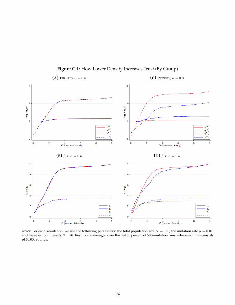
Figure C.1: How Lower Density Increases Trust (By Group)

(A) PROFITS, α = 0.5

(B) p, r, α = 0.5

(C) PROFITS, α = 0.8

(D) p, r, α = 0.5

Notes: For each simulation, we use the following parameters: the total population size N = 100, the mutation rate µ = 0.01,and the selection intensity β = 20. Results are averaged over the last 80 percent of 50 simulation runs, where each run consistsof 50,000 rounds.

82

Figure C.2: Investors’ Strategies: p vs. p

(A) p1 , α = 0.5

(B) p0 , α = 0.5

(C) p1 , α = 0.8

(D) p0 , α = 0.8

(E) p1 , α = 0.5

(F) p0 , α = 0.5

(G) p1 , α = 0.8

(H) p0 , α = 0.8

Notes: For each simulation, we use the following parameters: the total population size N = 100, the mutation rate µ = 0.01,and the selection intensity β = 20. Results are averaged over the last 80 percent of 50 simulation runs, where each run consistsof 50,000 rounds.

83